Spectral Function Calculation for Strongly Correlating Systems

Spectral Function Calculation for Strongly

Correlating Systems

Dissertation

zur Erlangung des Doktorgrades

des Fachbereichs Physik

der Universitat Hamburg

vorgelegt von

German Ulmaus

Krasnoyarsk

Hamburg2010

Gutachter der Dissertation Prof. Dr. A. Lichtenstein

Prof. Dr. M. Potthoff

Gutachter der Disputation Prof. Dr. A. Lichtenstein

Prof. Dr. E. Koch

Datum der Disputation 09 Juli 2010

Vorsitzender des Prufungsausschusses Dr. A. Chudnovskiy

Vorsitzender des Promotionsausschusses Prof. Dr. Jochen Bartels

Dekan des Fachbereichs Physik Prof. Dr. Heinrich Graener

Abstract

This thesis presents an efficient approach to calculate dynamical propertiesof solids with strong electron correlations. The fast cluster method, a so-called finite temperature Lanczos method is combined with the Dynamicalmean-field theory (DMFT) in order to study orbital degenerate systems asfunction of temperature. The full local Coulomb interaction was taken intoaccount in all calculations. A first application is two test systems: 5 + 1 and5 + 5 Anderson impurity models.

In the case of 5 + 1 Anderson impurity model it is possible to take intoaccount a large number of eigenstates: Narnoldi > 100. The chemical potentialof the system µ were changed in a broad range which leads to a change of amultiplet structure of the spectrum. In all this range of chemical potentialµ the ground state of the system is degenerate. At zero temperature itwere found that the temperature Lanczos calculations reproduce the correctdensity of states obtained with exact diagonalization if one chooses the set ofground states which remains the symmetry of the system. If all degenerateground states are taken into account than the temperature Lanczos methodreproduces the correct density of states of the test systems with a goodaccuracy.

In the case of finite temperaure calculations electron transitions to higherenergy levels become important. Therefore calculations with Narnoldi = 1 donot reproduce the DOS obtained with exact diagonalitation at any param-eters. One needs to consider not only the ground state but also low-energyexcited states.

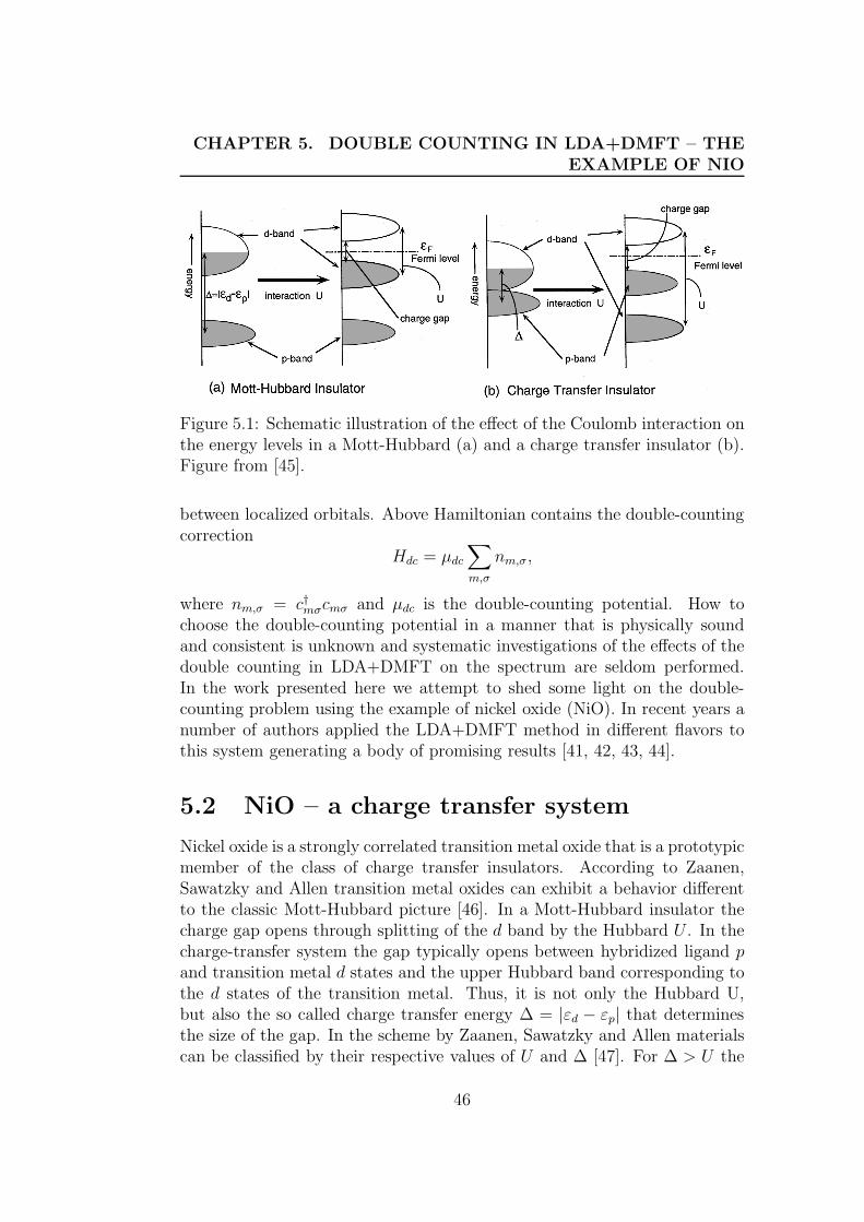
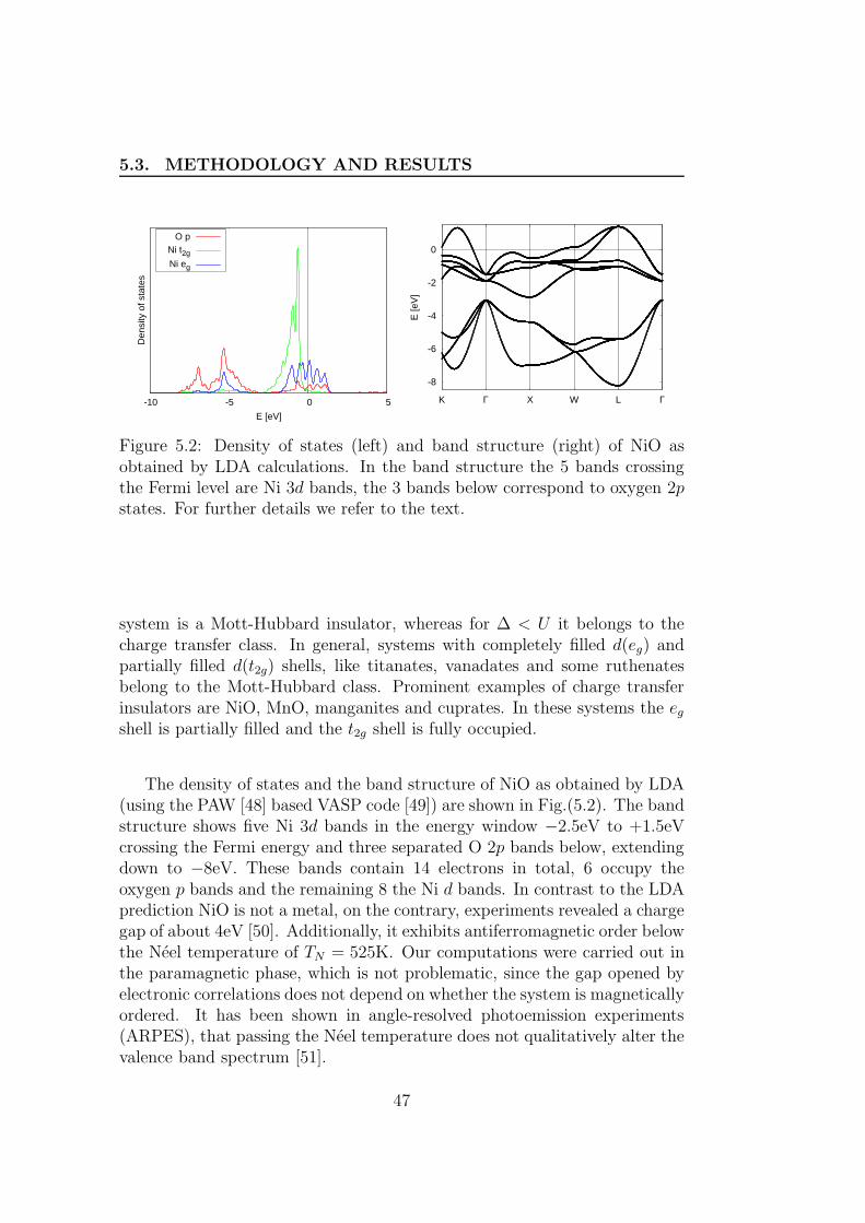
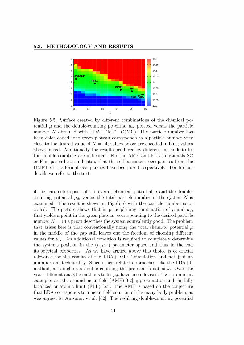
In the second part of the thesis the problem known as double-countingone for systems with strong electron correlations is considered. We conductedan extensive study of the charge transfer system NiO in the LDA+DMFTframework using quantum Monte Carlo and temperature Lanczos impuritysolvers. By treating the double-counting correction as an adjustable param-eter we systematically investigated the effects of different choices for thedouble counting on the spectral function. Different methods for fixing thedouble counting correction can drive the result from Mott insulating to al-

iii

most metallic. We propose a reasonable scheme for determination of thedouble-counting corrections for insulating systems.

The last part of the thesis describes the application of the LDA+DMFTapproach with the temperature Lanczos as impurity solver to the ferromag-netic nickel. The multiplet structure of full d-shell is taken into account. Asatellite peak in spectral function is found around −5 eV .

iv

Zusammenfassung

In dieser Doktorarbeit soll eine effiziente Methode zur Berechnung dynamis-cher Eigenschaften von Festkrpern mit starken elektronischen Korrelatio-nen prsentiert werden. Die Fast-Cluster-Methode, ein sogenanntes finite-temperature Lanczos, wurde mit der Dynamischen Molekularfeldtheorie (DMFT)kombiniert, um das Verhalten von Systemen mit entarteten Orbitalen in Ab-hngigkeit von der Temperatur zu untersuchen. In allen Rechnungen wurdedie volle lokale Coulombwechselwirkung bercksichtigt. Als erste Anwendungwurden zwei Testsysteme untersucht:5 + 1 und 5 + 5 Anderson-Impurity-Modelle.

Im Fall des 5+ 1 Anderson-Impurity-Modells ist es mglich, eine groe An-zahl von Eigenzustnden zu bercksichtigen: Narnoldi > 100. Das chemischePotential des Systems µ wurde ber einen groen Wertebereich hinweg vari-iert, was zu einer nderung der Multiplettstruktur des Spektrums fhrt. Imgesamten Wertebereich von µ ist der Grundzustand des Systems entartet.Es wurde festgestellt, da finite-temperature Lanczos die aus exakter Diago-nalisierung erhaltene korrekte Zustandsdichte reproduziert wenn man einenSatz von Grundzustnden whlt die die Symmetrie des Systems wahren. Wer-den alle entarteten Grundzustnde des Systems mitbercksichtigt, so repro-duziert finite-temperature Lanczos mit einer guten Genauigkeit die korrekteZustandsdichte.

Im Falle endlicher Temperaturen gewinnen die bergnge von Elektronen zuhheren Energieniveaus an Bedeutung. Daher reproduzieren Rechnungen mitNarnoldi = 1 fr keinen Satz von Parametern die korrekte Zustandsdichte. Esmssen zustzlich zu dem Grundzustand niederenergetische angeregte Zustndemitbercksichtigt werden.

Im zweiten Teil dieser Arbeit wurde ein als Double-Counting bekan-ntes Problem fr Systeme mit starken elektronischen Korrelationen nher be-trachtet. Wir fhrten im Rahmen von LDA+DMFT eine sorgfltige Unter-suchung des charge-transfer-Systems NiO durch, und zwar unter Verwendungdes Quantum Monte Carlo sowie des finite-temperature Lanczos ImpuritySolvers. Indem wir die Double-Counting-Korrektur als einen einstellbaren

v

Parameter behandelten untersuchten wir deren Einfluss auf die Spektral-funktion. Unterschiedliche Methoden zur Bestimmung des Double-Countingsknnen das Ergebnis von einem Mott-isolierenden bis hin zu einem nahezumetallischen Zustand ndern. Wir schlagen eine geeignete Methode zur Bes-timmung des Double-Countings in einem isolierenden System vor.

Der letzte Teil dieser Arbeit beschreibt die Anwendung von LDA+DMFTmit dem finite-temperature Lanczos als Impurity Solver auf ferromagnetis-ches Nickel. Die Multiplett-Struktur der vollen d-Schale wird dabei mitber-cksichtigt. Wir finden einen Satellit-Peak in der Spektralfunktion bei etwa−5 eV .

vi

Contents

1 Introduction 1

2 Density Functional Theory, Linear Muffin-Tin Orbitals 52.1 Thomas-Fermi approximation . . . . . . . . . . . . . . . . . . 52.2 The Hohenberg-Kohn theorems . . . . . . . . . . . . . . . . . 62.3 LSDA approximation . . . . . . . . . . . . . . . . . . . . . . . 102.4 Linear Muffin-Tin Orbital (LMTO) formalism . . . . . . . . . 10

3 Dynamical Mean-Field Theory 153.1 Exact Diagonalization . . . . . . . . . . . . . . . . . . . . . . 193.2 Quantum Monte Carlo method. Hyrsch-Fye algorithm . . . . 20

4 Finite Temperature Lanczos Method 254.1 The Lanczos method . . . . . . . . . . . . . . . . . . . . . . . 284.2 Dynamical properties . . . . . . . . . . . . . . . . . . . . . . . 31

4.2.1 Zero temperature . . . . . . . . . . . . . . . . . . . . . 314.2.2 Finite Temperature . . . . . . . . . . . . . . . . . . . . 35

4.3 Test calculations . . . . . . . . . . . . . . . . . . . . . . . . . 36

5 Double Counting in LDA+DMFT – The Example of NiO 455.1 Introduction . . . . . . . . . . . . . . . . . . . . . . . . . . . . 455.2 NiO – a charge transfer system . . . . . . . . . . . . . . . . . 465.3 Methodology and Results . . . . . . . . . . . . . . . . . . . . . 48

6 Satellite in Ni 556.1 Introduction . . . . . . . . . . . . . . . . . . . . . . . . . . . . 556.2 Methodology and Results . . . . . . . . . . . . . . . . . . . . . 56

7 Conclusions and Outlook 63

vii

CONTENTS CONTENTS

viii

Chapter 1

Introduction

Describing material properties from the ”first principles” using only infor-mation about the atomic structure is a great challenge in theoretical physics.The starting point of the ”theory of everything” is the Hamiltonian for thesystem of electrons and nuclei,

H = He + Hi + Hei (1.1)

where He describes the dynamics of electrons, Hi the ion core or nuclei, andHei their mutual interactions, . The Hamiltonian called ”ab-initio” containsonly the fundamental constants such as electronic charge, electronic and nu-clei masses etc. The nonreletevistic version of this Hamiltonian reads:

H = −~

2

2me

∑

i

∇2i −

∑

i,I

ZIe2

|ri − RI|+

1

2

∑

i6=j

e2

|ri − rj|

−∑

I

~2

2MI∇2

I +1

2

∑

I 6=J

ZIZJe2

|RI −RJ|,

(1.2)

where e, me, ri denote correspondingly electron charge, mass, coordinate andin analogy ZI , MI , RI are ion charge, mass and coordinate.

It is essential to include the effects of difficult many-body terms, namelyelectron-electron Coulomb interactions and the complex structures of thenuclei that emerge from the combined effects of all the interactions. Thegoal of the theory of electronic structure calculations the development ofmethods to treat electronic correlations with sufficient accuracy that one canpredict the diverse physical phenomena exhibited in matter, starting from(1.2). It is most informative and productive to start with the fundamentalmany-body theory.

There is only one type of term in the general Hamiltonian that can beregarded as ”small”, the ratio of electron mass to nuclei one me/MI . A per-turbation series can be defined in terms of this parameter which is expected

1

CHAPTER 1. INTRODUCTION

to have general validity for the full interacting system of electrons and nu-clei. In the first order approximation in me/MI the kinetic energy of thenuclei can be ignored. This is the Born-Oppenheimer or adiabatic approx-imation, which is an excellent approximation for many proposes, e.g. thecalculation of nuclear vibrations modes in different solids. In other cases,it forms the starting point for perturbation theory in electron-phonon inter-actions which is the basis for understanding electrical transport in metals,polaron formation in insulators, certain metal-insulator transitions, and theBCS theory of superconductivity. In this work we focus on the Hamiltonianfor the electrons, in which the positions of the nuclei are fixed.

Ignoring the nuclei kinetic energy, the fundamental Hamiltonian for thetheory electronic structure can be written as

H = T + Vext + Vint + EII (1.3)

If we adopt the Hartree atomic units ~ = me = 1, then the different termsin (1.3) may be written the simplest form. The kinetic energy operator forthe electrons T is

T = −1

2

∑

i

∇2i , (1.4)

Vext is the potential acting on the electrons due to the nuclei,

Vext =∑

i,I

VI(|ri − RI|), (1.5)

Vint is the electron-electron interaction,

Vint =1

2

∑

i6=j

1

|ri − rj|, (1.6)

and the final term EII is the classical interaction of nuclei with one anotherand contribute to the total energy of the system but are not important forthe problem of describing the electrons. Here the effect of nuclei the electronsis included in fixed potential ”external” to the electrons. Other ”external po-tentials”, such as electric fields and Zeeman terms, can readily be included.Thus, for electrons, the Hamiltonian, (1.3), is central to the theory of elec-tronic structure.

The fundamental equation governing a non-relativistic quantum systemis the time-independent Schrodinger equation,

HΨ(ri) = EΨ(ri), (1.7)

2

where the many-body wave function for the electrons is Ψ(ri) ≡ Ψ(r1, r2, . . . , rN),the spin is assumed to be included in the coordinate ri, and, of course, thewave function must be antisymmetric in the coordinates of the electronsr1, r2, . . . , rN .

The expression for any observable is an expectation value of an operatorO, which involves an integral over all coordinates,

〈O〉 =〈Ψ|O|Ψ〉

〈Ψ|Ψ〉. (1.8)

The density of particles n(r), which plays a central role in electronic structuretheory, is given by the expectation value of the density operator n(r) =∑

i=1,N δ(r − ri),

n(r) =〈Ψ|n(r)|Ψ〉

〈Ψ|Ψ〉= N

∫

d3r2 · · · d3rN

∑

σ1|Ψ(r1, r2, . . . , rN)|2

∫

d3r2 · · · d3rN |Ψ(r1, r2, . . . , rN)|2, (1.9)

which has this form because of the symmetry of the wave function in all theelectrons coordinates. (The density for each spin results if the sum over σ1

is omitted.) The total energy is the expectation value of the Hamiltonian,

E =〈Ψ|H|Ψ〉

〈Ψ|Ψ〉≡ 〈H〉 = 〈T 〉 + 〈Vint〉 +

∫

d3rVext(r)n(r) + EII , (1.10)

where the expectation value of the external potential has been explicitlywritten as a simple integral over the density function. The final term EII isthe electrostatic nucleus-nucleus (or ion-ion) interaction, which is essentialonly in the total energy calculation, but is just a classical additive term inthe theory of electronic structure.

The eigenstates of the many-body Hamiltonian are stationary points (sad-dle points or the minimum) of the energy expression (1.10). These may befound by varying the ration in (1.10) or by the varying the nominator subjectto the constraint of orthonormality (〈Ψ|Ψ〉 = 1), which can be done usingthe method of Lagrange multiplies,

δ[〈Ψ|H|Ψ〉 − E(〈Ψ|Ψ〉 − 1)] = 0. (1.11)

This is equivalent to the well-known Rayleigh-Ritz principle that functional

ΩRR = 〈Ψ|H − E|Ψ〉 (1.12)

is stationary at any eigensolution |Ψm〉. Variation of the bra 〈Ψ| leads to

〈δΨ|H − E|Ψ〉. (1.13)

3

CHAPTER 1. INTRODUCTION

The ground state wave function Ψ0 is the state with lowest energy, which canbe determined , in principle, by minimizing the total energy with respect to allthe parameters in Ψ(ri), with the constraint that Ψ must obey the particlesymmetry and any conservation laws. Excited states are saddle points of theenergy with respect to variations in Ψ.

4

Chapter 2

Density Functional Theory,Linear Muffin-Tin Orbitals

2.1 Thomas-Fermi approximation

The density functional theory of quantum systems is originated from thework of Thomas [1] and Fermi [2] written in 1927. Although their approx-imation is not accurate enough for present day electronic structure calcu-lations, the approach illustrates the main idea of functional theory. In theoriginal Thomas-Fermi method the kinetic energy of the system of electronsis approximated as an explicit functional of the density, idealized as noninter-acting electrons in homogeneous gas with density equal to the local densityat any given point. Both Thomas and Fermi neglected exchange and corre-lation among the electrons; however, this was extended by Dirac [3] in 1930,who formulated the local approximation for exchange still in use today. Thisleads to to the energy functional for electrons in an external potential Vext(r)

ETF =C1

∫

d3rn(r)(5/3) +

∫

d3r Vext(r)n(r)

+ C2

∫

d3r, n(r)(4/3) +1

2

∫

d3rd3r′n(r)n(r′)

|r − r′|,

(2.1)

where the first term is the local approximation to the kinetic energy withC1 = 3

10(3π2)(2/3) = 2.871 in atomic units, the third term is the local exchange

with C2 = −34( 3

π)(1/3)

and the last term is the classical electrostatic Hartreeenergy.

The ground state energy and electronic density can be found by minimiz-ing the functional E[n] in (2.1) for all possible n(r) subject to the constraint

5

CHAPTER 2. DENSITY FUNCTIONAL THEORY, LINEARMUFFIN-TIN ORBITALS

on the total number of electrons∫

d3rn(r) = N. (2.2)

Using the method of Lagrange multipliers, the solution can be found by anunconstrained minimization of the functional

ΩTF [n] = ETF [n] − µ

∫

d3r n(r) −N, (2.3)

where the Lagrange multiplier µ is the Fermi energy. For small variations ofthe density δn(r), the condition for a stationary points is

∫

d3rΩTF [n(r) + δn(r)] − ΩTF [n(r)] →∫

d3r5

3C1n(r)2/3 + V (r) − µδn(r) = 0,

(2.4)

where V (r) = Vext(r) + VHartree(r) + Vx(r) is the total potential. Since (2.4)must be satisfied for any function δn(r), it follows that the functional isstationary if and only if the density and potential satisfy the relation

1

2(3π2)(2/3)n(r)2/3 + V (r) − µ = 0. (2.5)

2.2 The Hohenberg-Kohn theorems

The achievement of Hohenberg and Kohn is the formulation of density func-tional theory as an exact theory of many-body systems. The formulationapplies to any system of interacting particles in external potential Vext(r),including any problem of electrons and fixed nuclei, where the Hamiltonianca be written

H = −~2

2me

∑

i

∇2i +

∑

i

Vext(ri) +1

2

∑

i6=j

e2

|ri − rj|. (2.6)

Density functional theory is based upon two theorems first provided by Ho-henberg and Kohn [4].Theorem 1: For any system of interacting particles in an external potentialVext(r), the potential Vext(r) is determined uniquely, except for a constant,by the ground state particle density n0(r).Theorem 2: A universal functional for the energy E[n] in terms of the den-sity n(r) can be defined, valid for any external potential Vext(r). For any

6

2.2. THE HOHENBERG-KOHN THEOREMS

particular Vext(r), the exact ground state energy of the system is the globalminimum value of this functional, and the density n(r) that minimize thefunctional is the exact ground state density n0(r).

Density functional theory is the most widely used method today for elec-tronic structure calculations because of the effective approach proposed byKohn and Sham in 1965: to replace the original many-body problem by anauxiliary independent-particle problem. This ansatz, in principle, leads toexact calculations of many-body systems using independent-particle meth-ods; in practice, it has made possible to approximate the DFT formulationthat have proved to be remarkably successful. As a self-consistent method.the Kohn-Sham approach involves independent particles but an interactingdensity, an appreciation of which clarifies the way the method is used.

In the Kohn-Sham approach one replaces the difficult interacting many-body system being described the Hamiltonian (1.2) with a different auxiliarysystem that can be solved more easily. Since there is no unique prescriptionfor choosing the simpler auxiliary system, this is an ansatz that rephrasesthe issues. The ansatz of Kohn and Sham assumes that the ground statedensity of the original interacting system is equal to that of some chosennon-interacting system that can be considered exactly soluble (in practiceby numerical QMC scheme) with all the difficult many-body terms incor-porated into an exchange-correlation functional of the density. By solvingthe equations one finds the ground state density and energy of the originalinteracting system with the accuracy limited only by the approximations inthe exchange-correlation functional.

Indeed, the Kohn-Sham approach has led to very useful approximationsthat are now the basis of most calculations that attempt to make ”first-principles” predictions for the properties of condensed matter and largemolecular systems. The local density approximations (LDA) or variousgeneralized-gradient approximations (GGA) are remarkably accurate, mostnotably for ”wide-band” systems, such as the group II and II-IV semicon-ductors, sp-bounded metals like Na and Al, insulators like diamond, NaCl,and molecules with covalent and/or ionic bonding.

The Kohn-Sham construction of an auxiliary system based on two as-sumptions.1. The exact ground state density can be represented by the ground statedensity of an auxiliary system of non-interacting particles. This is called”non-interacting-V-representability” ; although there are no rigorous proofsfor real systems of interest, we will proceed assuming its validity.

7


2.The auxiliary Hamiltonian is chosen to have the usual kinetic operatorand an effective local potential V σ

eff(r) acting on an electron of spin σ at pointr. The local form is not essential, but it is an extremely useful simplificationthat is often taken as the defining characteristic of the Kohn-Sham approach.

The actual calculations are performed on the auxiliary independent-particlesystem defined by the auxiliary Hamiltonian(using Hartee atomic units)

Hσaux = −

1

2∇2 + V σ(r). (2.7)

At this point the form of V σ(r) is not specified and the expressions mustapply for all V σ(r) in some range, in order to define functionals for a rangeof densities. For a system of N = N↑ + N↓ independent electrons obeyingthis Hamiltonian, the ground state has one electron in each of the Nσ orbitalsψσ

i (r) with the lowest eigenvalues ǫσi of the Hamiltonian (2.7). The densityof the auxiliary system is given by sums of squares of the orbitals for eachspin

n(r) =∑

σ

n(r, σ) =∑

σ

Nσ∑

i=1

|ψσi (r)|2, (2.8)

the independent-particle kinetic energy Ts is given by

Ts = −1

2

∑

σ

Nσ∑

i=1

〈ψσi |∇

2|ψσi 〉 =

1

2

∑

σ

Nσ∑

i=1

∫

d3r|ψσi (r)|2, (2.9)

and we define the classical Coulomb interaction energy of the electron densityn(r) interacting with itself

EHartree[n] =1

2

∫

d3rd3r′n(r)n(r′)

|r − r′|. (2.10)

The Kohn-Sham approach to the full interacting many-body problem is torewrite the Hohenberg-Kohn expression for the ground state energy func-tional in the form

EKS = Ts[n] +

∫

dr Vext(r)n(r) + EHartree[n] + EII + Exc[n]. (2.11)

Here Vext(r) is the external potential due to the nuclei and other externalfields(assumed to be independent of spins) and EII is the interaction be-tween the nuclei.

8

2.2. THE HOHENBERG-KOHN THEOREMS

Solution of the Kohn-Sham auxiliary system for the ground state can beviewed as the problem of minimization with respect to either the densityn(r, σ) or the effective potential V σ

eff(r). Since Ts is explicitly expressedas the functional of the orbitals but all other terms are considered to befunctionals of the density, one can vary the wave functions and use the chainrule to derive the variational equation

δEKS

δψσ∗i (r)

=δTs

δψσ∗i (r)

+

[

δEext

δn(r, σ)+δEHartree

δn(r, σ)+

δExc

δn(r, σ)

]

δn(r, σ)

δψσ∗i (r)

= 0, (2.12)

subject to the orthonormalization constraints

〈ψσi |ψ

σ′

j 〉 = δi,jδσ,σ′ . (2.13)

This is equivalent to the Rayleigh-Ritz principle [5, 6].Using expressions (2.8) and (2.9) for nσ(r) and Ts, which give

δTs

δψσ∗i (r)

= −1

2∇2ψσ

i (r);δnσ(r)

δψσ∗i (r)

= ψσi (r), (2.14)

and the Lagrange multiplier method for handling the constraints:

δ[〈Ψ|H|Ψ〉 −E(〈Ψ|Ψ〉 − 1)] = 0

〈δΨ|H − E|Ψ〉 = 0

this leads to the Kohn-Sham Schrodinger-like equations:

(HσKS − εσ

i )ψσi (r) = 0, (2.15)

where the εi are the eigenvalues, and HσKS is the effective Hamiltonian(in

Hartree atomic units)

HσKS(r) = −

1

2∇2 + V σ

KS(r), (2.16)

with

HσKS(r) = Vext(r) +

δEHartree

δn(r, σ)+

δExc

δn(r, σ)

= Vext(r) + VHartree(r) + V σxc(r).

(2.17)

Equations (2.15)-(2.17) are well-known Kohn-Sham equations, with the re-sulting density n(r, σ) and total energy EKS given by (2.8) and (2.11). Theequations have the form of independent-particle equations with a potentialthat must be found self-consistently with the resulting density. These equa-tions are independent of any approximations to the functional Exc[n], andwould lead to the exact ground state density and energy for the interactingsystem, if the exact functional Exc[n] were known.

9


2.3 LSDA approximation

Solids can be often be considered as close to the limit of the homogeneouselectron gas. In that limit, it is known that effects of exchange and correlationare local in character, and local density approximation(or more generallythe local spin density approximation (LSDA)), is reasonable, in which theexchange-correlation energy at each point assumed to be the same as inhomogeneous electron gas with that density,

ELSDAxc [n↑, n↓] =

∫

d3rn(r)ǫhomxc (n↑(r), n↓(r))

=

∫

d3rn(r)[ǫhomx (n↑(r), n↓(r)) + ǫhom

c (n↑(r), n↓(r))].

(2.18)

The LSDA can be formulated in terms of either two spin densities n↑(r) andn↓(r), or the total density n(r) and the fractional spin polarization ζ(r)

ζ(r) =n↑(r) − n↓(r)

n(r). (2.19)

The LSDA is the most general local approximation. For unpolarized systemsthe LDA is found simply by setting n↑(r) = n↓(r) = n(r)/2.

2.4 Linear Muffin-Tin Orbital (LMTO) for-

malism

The LMTO’s calculation scheme [7] is based on the concept of muffin-tinpotential which has proven to be a highly successful approximation of po-tential of realistic close-packed systems. In this concept the potential for asolid is approximated by a non-overlapping atomic-like spherical symmetricpotential inside a sphere with radius S, and a constant in the interstitialregion

V (r) =

V (|r|), r ≤ S

Vc, r > S.(2.20)

Therefore, the Schrodinger equation can be solved exactly in both regions(r ≤ S and r > S). These solutions are matched at the sphere boundariesto produce the muffin-tin orbitals. To reduce the effect of interstitial regionone introduces the overlapping atomic spheres which fill the whole volume ofthe crystal. In this, the so-called Atomic Sphere Approximation (ASA), the

10

2.4. LINEAR MUFFIN-TIN ORBITAL (LMTO) FORMALISM

volume of interstitial region equals to zero, i.e., the electron kinetic energyκ2 = ε−Vc in this region becomes a free parameter which can be taken equalto zero. In this case wave function inside a sphere (for r ≤ S) satisfies to theradial Schrodinger equation, whereas outside it corresponds to the solutionof Laplace equation ∇2Φ = 0. Therefore, the radial part of the wave functioncan be written as

Φl(r, ε) =

ul(r, ε), r ≤ S

[

Dl+l+12l+1

( rS)l + l−Dl

2l+1( r

S)−l−1

]

ul(S, ε), r > S,(2.21)

where ul(r, ε) is the exact radial solution of Schrodinger equation which isnormalized by one in the MTO sphere with radius S. These functions are notconvenient to use as basis functions because of its divergence for large r. Inorder to construct decaying for large r, continuous and smooth in the wholespace basis functions one has to substract the divergent wave Dl+l+1

2l+1( r

S)l from

both parts of (2.21)

Φl(r,D) =

Φ(r,D) − D+l+12l+1

Φl(S,D)Φl(S,l)

Φl(r, l), r ≤ S

l−D2l+1

[ rS]−l−1 Φl(S,D), r > S,

(2.22)

where DL(ε) is the logarithmic derivative of the radial part of wave functionat the sphere radius S

DL(ε) = Sul(r, ε)

ul(r, ε)

∣

∣

∣

r=S. (2.23)

The obtained functions are not (any more) the solutions of Schrodinger equa-tion inside the atomic sphere. However, it is convenient to use them to builtup the Bloch sums of the crystal. Taking into account all tails of basis func-tions from the other sites in central sphere at Rs, the Bloch sums can bewritten as

χk

L(r, D) =∑

Rs 6=0

eik·Rs ΦL(r − Rs, D), (2.24)

where tails from the center with radius-vector RS are defined by

ΦL(r − Rs, D) = ilYL(r − Rs)∣

∣

∣

r − Rs

S

∣

∣

∣

−l−1 l −D

2l + 1Φl(S,D). (2.25)

Taking tails expansion in partial waves at the center of sphere and makingthe Bloch basis functions continuous and differentiable on the sphere surface,

11


one obtains

χk

L(r, D) =

ΦL(r, D) − Φl(S,D) l−D2l+1

∑

L′

[

Sk

L′L − D+l+1l−D

×

×2(2l + 1) δLL′

]

ΦL′(r,l′)

2(2l′+1)Φl′ (S,l′), r ≤ S,

Φl(S,D) l−D2l+1

[

ilYL(r)( rS)−l−1 +

∑

L′ Sk

L′L×

×il′

YL′(r)( rS)l′ 1

2(2l′+1)

]

, r > S.

(2.26)

Here, χk

L(r, D) are the so-called muffin-tin orbitals, and Sk

L′L are the struc-tural constants which are defined via

Sk

LL′ =∑

R

eik·RSR

LL′, and

SR

LL′ = −8π(2l + 2l′ − 1)!!

(2l − 1)!!(2l′ − 1)!!

∑

L′′

CLL′′L′(−i)l′′(R

S

)−l′′−1

YL′′(R),(2.27)

where CLL′′L′ are the Gaunt’s coefficients. YL(R) are the correspondingspherical harmonics. The solution of Schrodinger equation of the whole crys-tal is a linear combination of MT-orbitals

Ψk(r) =∑

L

CL(k)∑

Rs 6=0

eik·RS χk

L(r − RS, Dl(ε)) (2.28)

which must be exact solution of the radial Schrodinger equation inside ofatomic spheres. According to this condition all tails from other sites andunphysical terms in MT-orbital, that is proportional to [ilYL(r) rl], have toeliminate each other inside of all atomic spheres, i.e., the second term inχk

L(r, D) (Eq. 2.26) will turn to zero. This gives a set of linear homogeneousequations

∑

L

(Sk

LL′ − δLL′Pl(ε))CL(k)Φl(S,Dl) = 0, (2.29)

where the total information about crystal potential is included in the poten-tial functions

Pl(ε) = 2(2l + 1)Dl(ε) + l + 1

Dl(ε) − l. (2.30)

The crystal structure information is contained in the structural constantsSk

LL′ (Eq. 2.27). Therefore, the main problem of band structure calculations isto find eigenvalues and eigenvectors for single atomic sphere with spherically

12

2.4. LINEAR MUFFIN-TIN ORBITAL (LMTO) FORMALISM

symmetric potential and k-dependent boundary conditions which appearsfrom neighboring spheres. By construction the MTO basis set χk

L(r, D) isan energy dependent. This considerably complicates numerical evaluation ofthe secular equation whose solution defines the energy spectra of the system

det||〈χk

L(r, D)|H − εO|χk

L(r, D)〉|| = 0. (2.31)

Here, H and O are the Hamiltonian and overlap operators, respectively.To resolve such a difficulty the linear MTO (LMTO) method was intro-

duced which is based on the power expansion of the original MTO’s up tothe linear order in energy. The energy independent LMTO basis set providesa rapid convergence of the method. Taking into account only linear term inthe Taylor expansion for the MTO basis wave function in an arbitrary energypoint εν one obtains

Φ(r,D) = Φν(r) + w(D)Φν(R). (2.32)

Here, Φν(r) is the value of wave function at the energy point εν , i.e. Φν(r) =ul(εν, r). Φν(r) is the energy derivative of the wave function at the expansionpoint Φν(r) = ∂

∂εul(ε, r)|ε=εν

which is normalized by one in the atomic spherewith radius S. w(D) is calculated as follows

w(D) = −Φν(r)

Φν(r)

D −Dν

D −Dν

, (2.33)

where D is the logarithmic derivative on the atomic sphere surface

D =Φ′(r,D)

Φ(r,D)

∣

∣

∣

r=S.(2.34)

Dν and Dν are defined via Dν = S Φ′

ν(S)Φν(S)

and Dν = S Φ′

ν(S)

Φν(S), respectively.

The expansion energy point εν is selected within the region of energiesoccupied by the valence electrons which is obtained from the solution of theSchrodinger equation within the atomic sphere. Therefore, if we consider anarbitrary energy ε, then the LMTO’s have an error of order (ε− εν)

2 withinthe spheres.

In the LMTO basis set matrix elements of the Hamiltonian and overlapmatrix inside of sphere can be written as

〈Φ′L(D′, S)|H − ενO|ΦL(D,S)〉 = δL,L′ wl(D),

(2.35)

〈Φ′L(D′, S)|ΦL(D,S)〉 = δL,L′ (1 + 〈Φ2

νl|ΦL(D,S)〉wl(D)wl(D′)),

13


where ΦL(r,D) is orthogonal to Φν(r) because of the normalization condition〈Φ(r, ε)|Φ(r, ε)〉 = 1 and ∂

∂ε〈Φ(r, ε)|Φ(r, ε)〉 = 2〈Φ(r, ε)|Φ(r, ε)〉 = 0.

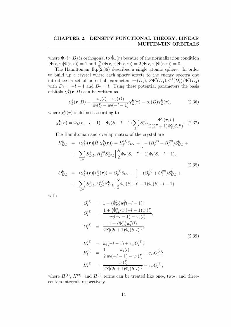
The Hamiltonian Eq.(2.36) describes a single atomic sphere. In orderto build up a crystal where each sphere affects to the energy spectra oneintroduces a set of potential parameters wl(D1), SΦ2(D1),Φ

2(D1)/Φ2(D2)

with D1 = −l − 1 and D2 = l. Using these potential parameters the basisorbitals χk

L(r, D) can be written as

χk

L(r, D) =wl(l) − wl(D)

wl(l) − wl(−l − 1)χk

L(r) = αl(D)χk

L(r), (2.36)

where χk

L(r) is defined according to

χk

L(r) = ΦL(r,−l − 1) − Φl(S,−l − 1)∑

L′

Sk

L′L

Φ′L(r, l′)

2(2l′ + 1)Φ′l(S, l

′)(2.37)

The Hamiltonian and overlap matrix of the crystal are

Hk

L′L = 〈χk

L′(r)|H|χk

L(r)〉 = H(1)l′ δL′L +

[

− (H(2)l′ +H

(2)l )Sk

L′L +

+∑

L′′

Sk

L′L′′H(3)L′′S

k

L′′L

]S

2Φl′(S,−l

′ − 1)Φl(S,−l − 1),

(2.38)

Ok

L′L = 〈χk

L′(r)|χk

L(r)〉 = O(1)l′ δL′L +

[

− (O(2)l′ +O

(2)l )Sk

L′L +

+∑

L′′

Sk

L′L′′O(3)L′′S

k

L′′L

]S

2Φl′(S,−l

′ − 1)Φl(S,−l − 1),

with

O(1)l = 1 + 〈Φ2

νl〉w2l (−l − 1);

O(2)l =

1 + 〈Φ2νl〉wl(−l − 1)wl(l)

wl(−l − 1) − wl(l);

O(3)l =

1 + 〈Φ2νl〉w

2l (l)

2S[(2l + 1)Φl(S, l)]2;

(2.39)

H(1)l = wl(−l − 1) + ενlO

(1)l ;

H(2)l =

1

2

wl(l)

wl(−l − 1) − wl(l)+ ενlO

(2)l ;

H(3)l =

wl(l)

2S[(2l + 1)Φl(S, l)]2+ ενlO

(3)l ,

where H(1), H(2), and H(3) terms can be treated like one-, two-, and three-centers integrals respectively.

14

Chapter 3

Dynamical Mean-Field Theory

The dynamical mean-field theory can be obtained in many ways [8], whichdiffer between each other for the mathematical formalism adopted and thedegree of complexity. The most pedagogical derivation starts probably froma comparison with the Weiss molecular field theory for the Ising model.

The Ising model is a lattice of classical spins Si described by the Hamil-tonian

H = −J∑

i,j

SiSj − h∑

i

Si, (3.1)

where h is the energy of single spin in an external(magnetic) field and J isthe ferromagnetic energy due to a spin-spin interaction. To keep the modelrealistic the first sum is limited to indexes that run for pairs of nearest neigh-bors. The presence of the interaction term correlates the spin between eachother. which makes the system hard to solve directly. However, if we focuson one physical quantity, we can try to reduce it to a simpler equivalentsystem that we are able to solve. Let us focus on the magnetization at site i

mi ≡ 〈Si〉, (3.2)

the is the thermal average of a spin at a single site. Our equivalent system isa lattice of non-interacting spins moving in an effective site-dependent fieldheff and the corresponding Hamiltonian is

Heff = −∑

i

heffi Si. (3.3)

The effective field should be chosen to reproduce the same magnetization mi

of the original lattice. Calculating the sum over all the possible configurationsfor (3.3), we can write down an explicit expression for the effective field:

βheffi = tanh−1mi, (3.4)

15

CHAPTER 3. DYNAMICAL MEAN-FIELD THEORY

where β = 1/kBT . Up to now we have not made any approximations, butwe still have not obtained a relation with the original system. In the Weissmean-field theory the effective field is approximated by the thermal averageof the local field seen by a spin at a given site:

heffi ≃ h + J

∑

j

〈Si〉 = h + Jzmi. (3.5)

In the last step we have contextualized our discussion to a translational in-variant system with z nearest neighbors for every site. The equation (3.4)and (3.5) can be solved analytically, leading to the approximated magnetiza-tion. We have to stress that the procedure of the mapping into an equivalentnon-interacting system is exact with respect to the chosen observable: theapproximation is made when establishing a relation between the Weiss fieldand the neighboring sites. Furthermore the approximation becomes exact inthe limit of z → ∞ [9]. This result is quite intuitive: the neighbors of a givensite can be globally treated as bath when their number becomes large.

All these ideas can be easily extended to the Hubbard model [10]. Being afully-interacting quantum many-body system, the mapping procedure is notas obvious as above, but can be established on rigorous basis. For simplicitywe consider the one-band Hubbard model [11, 12, 13]

Hhub = −t∑

R,R′

c+R,σ cR′,σ + U∑

R

nR,↑nR,↓. (3.6)

Instead of the magnetization, we focus on the local Green’s function at asingle site:

GσR,R′(τ − τ ′) ≡ −〈T cR,σ(τ)c+

R′,σ(τ′)〉. (3.7)

Here τ and τ ′ are imaginary times in the Matsubara’s formalism for the per-turbation theory at finite temperature and T is the time-ordering operator.

As before, we would like to chose the reference system as a single siteembedded in an effective field. Since the Green’s function (3.7) is time de-pendent, the new field must also evolve in time, i.e. must be dynamical.The simplest field we can imagine is a bath of non-interacting electrons. Thesingle site, the bath and their coupling can be described by the followingHamiltonian:

Heff = Hatom + Hbath + Hcoupling. (3.8)

The first termHatom = Uc+↑ c↑c

+↓ c↓ (3.9)

is the Coulomb repulsion of two electrons at the atomic site, and c, c+ are thecorresponding spin-dependent annihilation and creation operators. Notice

16

that this term comes directly from the initial equation (3.6). To assure aformal distinction between the operators of the original model and the latticemodel we have omitted the index R. The second term of the equation (3.8)is

Hbath =∑

k,σ

εk,σa+k,σak,σ (3.10)

and represents the fictitious sea of electrons whose quantum numbers aretheir spin σ and number of site in the bath k. We use a and a+ for the cor-responding annihilation and creation operators, and εk,σ for the bath orbitalenergies. Finally the last term of equation (3.8)

Hcoupling =∑

k,σ

Vk,σ(a+k,σ cσ + c+σ ak,σ), (3.11)

describes the exchange of electrons between site and bath at an energy εk,σ

with amplitude Vk,σ.The Hamiltonian (3.8) is a well-known problem in many-body physics: it

is a single impurity Anderson model . In the last 40 years it has been studiedextensively and nowadays can be solved through many methods, dependingon the range of the parameters and on the allowed approximations . By nowwe are interested in finding the connection of the parameters εk,σ and Vk,σ

with the full solution of the problem, i.e. the analogous formula to equation(3.4). To this aim we treat the first term of equation (3.8) as a perturbation[14]; then the other two terms determine the unperturbed Green’s function ofthe bathG0. Passing from the imaginary time τ to the Matsubara frequenciesiωi, we have

Gσ0 (iωn) =

1

iωn + µ− ∆σ(iωn)(3.12)

where µ is the chemical potential, which sets the correct number of particles,and the quantity

∆σ(iωn) =∑

k

|Vk,σ|2

iωn − εk

(3.13)

is called hybridization function. In terms of many-body perturbation theorythe full Green’s function of the Hamiltonian (3.8) can be obtained by meansof the Dyson equation

Gσimp = [Gσ

0 (iωn)−1 − Σσimp(iωn)]−1, (3.14)

where Σimp is the self-energy function and contains all the effects of theinteractions. Σimp depends only on the unperturbed Green’s function G0

and the interaction term equation (3.9). The parameters εk,σ and Vk,σ enter

17


in the full problem only through G0, which takes the meaning of the ”Weiss”field and which is determined to have the impurity full Green’s function (3.14)coincide with the local Green’s function (3.7):

Gσimp(iωn) = Gσ

R,R′(iωn). (3.15)

The fact the parameters do not appear explicitly in the mapping proceduremakes it more rigorous to redefine the problem in terms of an effective actionformalism [15], instead of the Hamiltonian (3.8). Integrating out the bathdegrees of freedom, we can write down the effective action for the orbital ofthe impurity as

S = −

∫ β

0

dτ

∫ β

0

dτ ′∑

σ

c+σ (τ)[Gσ0 (τ − τ ′)]−1cσ(τ

′)+

U

∫ β

0

dτ c+↑ (τ)c↑(τ)c+↓ (τ)c↓(τ). (3.16)

The action S fully determines the dynamics of the local site under consider-ation: the first term takes into account electrons jumping from the bath onthe site at τ and coming back to the bath at τ ′; the second term includesthe Coulomb repulsion when two electrons with opposite spins are presenton the site at the same time. Now we have the most rigorous expression forthe full Green’s function of the impurity:

Gσimp(τ − τ ′) ≡ −〈T cσ(τ)c+σ (τ ′)〉S. (3.17)

Anyway we must stress again that in both the formulations in terms ofDyson’s equation or in terms of the effective action, the central point isthe preservation relation (3.15).

Up to now the representation of the chosen observable of the originallattice is exact. The approximation is done with the next step: the connectionof the two systems. In the DMFT the lattice self-energy is only local andcoincides with the self-energy of the impurity model:

ΣσR,R′(iωn) = δR,R′Σσ

imp(iωn). (3.18)

In the reciprocal space it means that the self-energy becomes k-independent.While the approximation (3.18) can appear rather arbitrary,indeed is

mathematically very similar to equation (3.5). In fact it becomes exact in thelimit of infinite nearest neighboring sites, or equivalently, infinite dimensions,as was proved by Metzer and Vollhardt in a work [16] that is considered thefirst mile-stone of the DMFT. One year later, George and Kotliar [9] com-pleted the main framework of the theory by proving that in the same limit the

18

3.1. EXACT DIAGONALIZATION

Hubbard model can be exactly mapped into the Anderson impurity model.Their proof is based on the fact that the topology of all irreducible Feynmandiagrams becomes the same in the two systems: simply the local contri-bution of all the diagrams. The parallelism between the Weiss mean-fieldtheory for the classical Ising model and the quantum Hubbard model is sum-marized in Table 3. In addition we show also that the same representationcan be constructed for the Kohn-Sham equations. In this case the originalsystem is the many-electron Hamiltonian (1.2), and the mapping system isthe non-interacting electron gas (2.16) in the effective potential VKS. Theapproximation comes with the LDA exchange-correlation functional (2.18).It is clear that a strong mathematical connection exists between these gener-alized mean-field theories. More precisely all the three of them can be seenas generalization of the thermodynamical Legendre transformation

Before ending the Chapter we should emphasize that the convergenceof the DMFT approximation with respect to the number of neighbors isvery fast, and this makes it applicable also for more realistic cases, like a 3-dimensional solid. Moreover there are two other limits for which the DMFTbecomes exact:

• in the atomic limit t = 0 the sites are decoupled from each other, so thatthe hybridization function ∆(iωn) is zero; as a result the self-energy hasonly on-site component, i.e. it is local

• in the non-interacting limit U = 0 the self-energy becomes zero, andthen again trivially local.

Original System Ising Model Hubbard Model Electron HamiltonianMapping System Spins in a Single Impurity Electrons in an

Effective Field Anderson Model Effective PotentailSelected Observable Magnetization Green’s Function Electron Dencity

mi GR,R′(τ − τ ′) n(r)

Approximation heffi ≃ h + zZmi Σσ

R,R′ ≃ δR,R′Σσimp Exc[n] ≃ ELDA

xc [n]

3.1 Exact Diagonalization

Exact diagonalization methods are important tools for studying the physi-cal properties of quantum many-body systems. These methods typically areused to determine a few of the lowest eigenvalues and eigenvectors of mod-els of many-body systems on a finite lattice. From these eigenvalues andeigenvectors, various ground state expectation values and correlation func-tions are easily computed. Although the methods are limited to small lattice

19


sizes, they have become increasingly popular because of using with DMFT.In addition to provideng useful benchmarks for approximate theoretical cal-culations and quantum Monte Carlo simulations they help to provide insightinto the often subtle properties of unsolvable many-body problems in thethermodynamical limit.

The expression ”Exact diagonalization” is used to describe a number ofdifferent approaches [8, 17] which yield numerically exact results for a finitelattice system by directly diagonalizing the matrix representation of the sys-tem’s Hamiltonian in an appropriate many-particle basis. The simplest, andthe most time- and memory- consuming approach is the exact diagonalization[18, 19] of the matrix which enables one to calculate all desired properties.However, the dimension of the basis for a strongly interacting quantum sys-tems grows exponentially with the system size, so it is impossible to treatsystems with more than a few sites. If only properties of low- or high-lyingeigenstates are required, (in the investigation of condensed matter systemsone is often interested in the low-energy properties), it is possible to reachsubstantially larger system sizes using iterative diagonalization procedures,which also yields result to almost machine precision in most cases. Theiterative diagonalization methods allow for the calculation of ground stateproperties and (with some extra efforts) some low-lying excited states are alsoaccessible. In addition, it is possible to calculate dynamical properties (e.g.spectral functions, time evaluation) as well as behavior a finite temperature.Nearly every system and observable can be calculated in principle, althoughthe convergence properties may depend on the system under investigation.In chapter 4 we will describe such iterative method - the Lanczos algorithm- in details.

3.2 Quantum Monte Carlo method. Hyrsch-

Fye algorithm

The quantum Monte Carlo scheme is the most universal tool [20, 21] for thenumerically study of quantum many-body systems with strong correlations.The auxiliary-field scheme allows to deal with fermionic systems with strongelectronic correlations. The determinantal auxiliary-field algorithm, namelyHirsch-Fye appeared more than 20 years ago and became nowadays standardfor the numerical investigation [22, 23] of physical models with with stronginteractions, as well as for the quantum chemistry and nanoelectronics. Weregard this method as it is an efficient as impurity solver within DMFT ,i.e.in solving Anderson impurity model.

20

3.2. QUANTUM MONTE CARLO METHOD. HYRSCH-FYEALGORITHM

The one band single-impurity model is specified by the imaginary timeeffective action:

Seff = −

∫ β

0

dτdτ ′∑

σ

c+σ (τ)G−1σ (τ − τ ′)cσ(τ ′)

+

∫ β

0

dτUn↑(τ)n↓(τ′),

(3.19)

G−1σ (iω) = iω + µ− ∆σ(iω), (3.20)

where c+σ (τ) and cσ(τ) are Grassmann variables, µ denotes the chemical po-tential, U is on-site Coulomb repulsion and ∆σ(iω) is a hybridization functionthat describes transitions into the bath and back.

The aim of the impurity solver is to compute the Green’s function

G(τ − τ ′) = 〈Tτc+σ (τ)cσ(τ ′)〉Seff

=Tr[Tτe

−Seff c+σ (τ)cσ(τ ′)]

Tr[TτeSeff ](3.21)

for a given hybridization function.The first step in Hirsch-Fye algorithm is a discretization of the impurity

model effective action (3.19):

Seff →∑

ττ ′σ

c+σ (τ)G−1σ (τ − τ ′)cσ(τ ′) + Un↑(τ)n↓(τ

′), (3.22)

where the imaginary time is discretized in L ”slices” τ = 1, 2, . . . , L of size∆τ , and the time step ∆τ is defined by β = L∆τ .

We temporarily introduce the Hamiltonian description of the local im-purity problem, which permits a local in time description of the partitionfunction. In order to preserve the standard notations for this model, theimpurity orbital will be taken as a d orbital. The conduction bath orbitalsare numbered from p = 2, . . . , ns, and the impurity orbitals is equivalentlydenoted by c1σ ≡ dσ, i.e. corresponds to p = 1. The Hamiltonian of a generalAnderson impurity model reads

H =∑

p≥2,σ

εpc+pσcpσ +

∑

p≥2,σ

Vp(c+pσdσ + d+

σ cpσ)

εd

∑

σ

d+σ dσ + Und↑nd↓

(3.23)

It is written as a sum of terms H = H0 +H i, where H0 is a quadratic in thefermion operators:

H0 ≡∑

p≥2,σ

εpc+pσcpσ +

∑

p≥2,σ

Vp(c+pσdσ + d+

σ cpσ)

+ (εd + U/2)∑

σ

ndσ,(3.24)

21


whereas H i is a interaction term :

H i ≡ U [nd↑nd↓ −1

2(nd↑ + nd↓)]. (3.25)

The discretization allows to write a partition function as

Z = TrL∏

l=1

e−βH = Tre−∆τ [H0+Hi] (3.26)

The follow derivation is based on the Trotter-Suzuki transformation, namelyfor operators A and B

e(A+B) = limL→∞

(eA/LeB/L) (3.27)

This implies that exp(−∆τ(A+B)) = lim∆→0

exp(−∆τA)exp(−∆τB)+O(∆τ 2).

Hence the exponential of the Hamiltonian in (3.26) is approximately factor-ized into Gaussian and interacting parts up to an error of order O(∆τ 2) bydiscretizing the imaginary time interval into L slices:

Z ≃ Z∆τ ≡ TrL∏

l=1

e−∆τH0

e−∆τHint

(3.28)

The Green’s function corresponding to Z∆ can be defined analogously, byusing U∆τ ≡ exp(−∆τH0)exp(−∆τH i) and an evolution operator betweentime slices:

g∆τp1,p2

(τl1 , τl2) ≡ 〈ap1(τl1)a

+p2

(τl2)〉

=TrUL−l1

∆τ ap1(τl1)U

l1−l2∆τ a+

p2(τl2)U

l2∆τ

TrUL∆τ

, (3.29)

we l1 > l2 is supposed.The partition function is further evaluated by transforming the interact-

ing problem into a noninteracting one. This happens at the cost of intro-ducing auxiliary degrees of freedom and is facilitated by a discrete Hubbard-Stratonovich transformation [24, 25, 26], applied on each slices:

exp[−∆τH i] =1

2

∑

s=±1

exp[λs(nd↑ − nd↓)],

cosh(λ) ≡ exp(∆τU/2)

(3.30)

22

3.2. QUANTUM MONTE CARLO METHOD. HYRSCH-FYEALGORITHM

and after inserting (3.30) into (3.28), the partition function Z∆ is reduced to

Z∆ =1

2L

∑

s1,...,sL=±1

Z∆s1,...,sL

=1

2L

∑

s1,...,sL=±1

detO↑(S detO↓(S) (3.31)

with

Z∆s1,...,sL

=∏

σ=±1(=↑↓)

Tre−∆τH0

eV σ(s1)

× e−∆τH0

eV σ(s2) · · · e−∆τH0

eV σ(sL)

(3.32)

In equation (3.32), the ns × ns matrix V σ(s) is diagonal with

eV σ(s) =

eλσs · · · · · · 0· · · 1 · · · · · ·· · · · · · 1 · · ·· · · · · · · · · 1

(3.33)

The matrices Oσ(S have dimensions NsL × NsL and depend on the par-ticular configuration of the Ising spins denoted by S.

The crucial fact noted by Hirsch and Fye is that the Green’s functionsfor two different Ising spins configurations, (s1, . . . , sL) and (s′1, . . . , s

′L), are

related to each other by a Dyson equation. Abbreviating g ≡ g∆τs1,...,sL

andg′ ≡ g∆τ

s′1,...,s′

L, etc, this Dyson equation reads

g′ = g + (g − 1)(eV ′−V − 1)g′. (3.34)

In fact, Eq. (3.34) relates two Green’s functions g and g′ via a projectionoperator on the d site, namely [exp(V ′ − V ) − 1]. The presence of thisprojection operator comes from the possibility of the integrating out theconduction band. As a consequence, the Dyson equation (3.34) directly re-lates the Green’s functions on the d site one to another, and this equationremains equally valid in the subspace is = 1, i′s = 1. Hence, the d site Green’sfunctions G∆τ

s1,...,sLalso satisfy

G′ = G + (G− 1)(eV ′−V − 1)G′, (3.35)

viewed as an L× L matrix equation.Rearranging Eq. (3.35), it is straightforward to see that Gs′

1,...,s′

Lfor an

Ising configuration (s′1, . . . , s′L) can be obtained from Gs1,...,sL

by inversion ofan L× L matrix A, defined in the following equation

AG′ = G,A ≡ 1 + (1 −G)[eV ′−V − 1]. (3.36)

23


In the special case in which (s′1, . . . , s′L) differs from (s′1, . . . , s

′L) by the value

of a single spin, say sl, A takes on a special form

A =

1 0 A1l 0 · · ·0 1 A2l 0 · · ·· · · 0 All · · · · · ·· · · · · · · · · 1 0· · · · · · ALl 0 1

(3.37)

In that case, detA = All = 1 + (1 − Gll)[exp(V′l − Vl) − 1]. Expanding A−1

in minors, it can be easily be seen that A−1lk = 0 for k 6= l. In that case Eq.

(3.36) simplifies to

G′l1l2 = Gl1l2 + (G− 1)l1l(e

V ′−Vll − 1)(All)

−1Gll2 , (3.38)

which is a special case of a Sherman-Morrison formula [27]. equation (3.34)can be also be used to show that

detO′

detO=

detG

detG′

= detA = 1 + (1 −Gll)[exp(V′ − V ) − 1]

(3.39)

It is remarkable that all the equations (3.35-3.39) express exact relationsbetween discretized Green’s functions G∆τ . The only error left is related tothe Trotter-Suzuki decomposition.

24

Chapter 4

Finite Temperature LanczosMethod

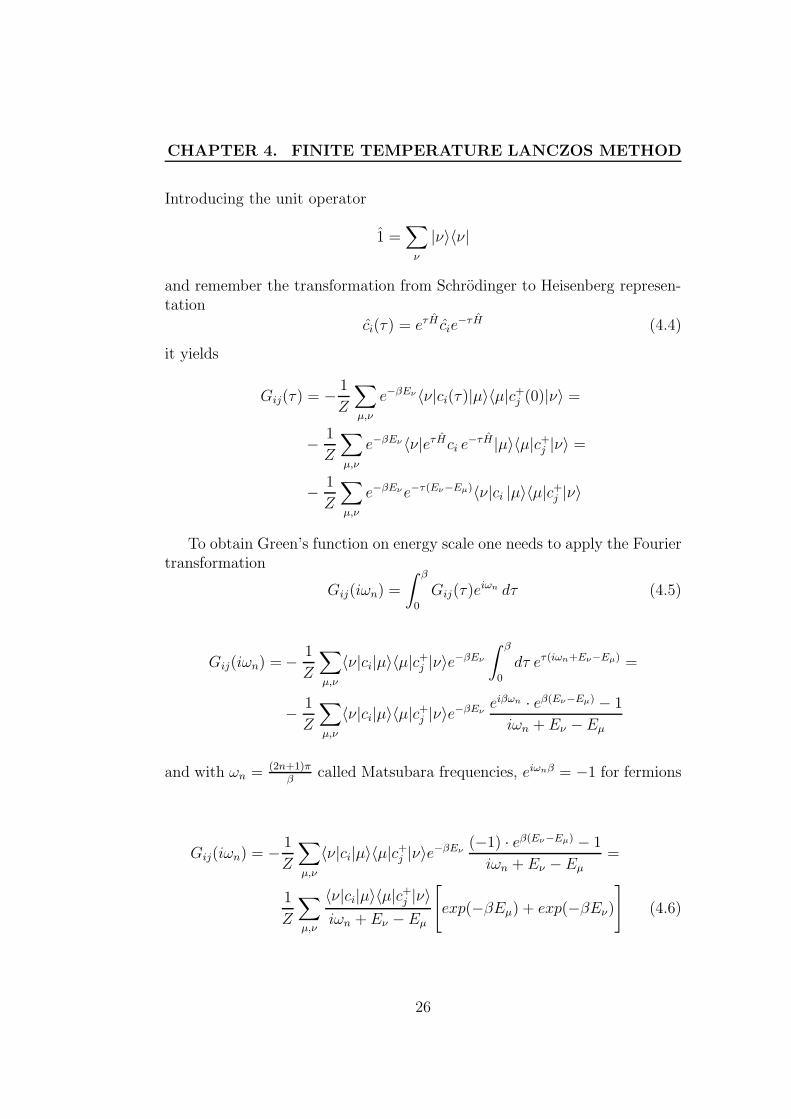
As was mentioned above the key quantity on which DMFT focuses is thelocal Green’s function. In the case of finite temperatures it is defined onimaginary time as follows [28]

Gij(τ) = −〈ci(τ)c+j (0)〉 = −

1

ZTre−βHci(τ)c

+j (0), (4.1)

where τ is imaginary time, c+i (τ), ci(τ) are creation and annihilation opera-tors acting on site with number i and defined in Heisenberg representation, βis inverse temperature and average is evaluated on grand canonical ensemble.

One of the advantages of Lanczos method is the capability to calculateGreen’s function on the real energies. It is due that the calculation is basedon the Lehmann representation of the Green’s function. We evaluate thisformula due to Mahan [29]. Using eigenvalues and eigenstates for the systemwith Hamiltonian H :

H|ν〉 = Eν |ν〉 (4.2)

the expression for Green’s function reads

Gij(τ) = −1

Z

∑

ν

〈ν|e−βHci(τ)c+j (0)|ν〉,

where Z is a partition function:

Z =∑

ν

e−βEν (4.3)

25

CHAPTER 4. FINITE TEMPERATURE LANCZOS METHOD

Introducing the unit operator

1 =∑

ν

|ν〉〈ν|

and remember the transformation from Schrodinger to Heisenberg represen-tation

ci(τ) = eτH cie−τH (4.4)

it yields

Gij(τ) = −1

Z

∑

µ,ν

e−βEν 〈ν|ci(τ)|µ〉〈µ|c+j (0)|ν〉 =

−1

Z

∑

µ,ν

e−βEν 〈ν|eτHci e−τH |µ〉〈µ|c+j |ν〉 =

−1

Z

∑

µ,ν

e−βEνe−τ(Eν−Eµ)〈ν|ci |µ〉〈µ|c+j |ν〉

To obtain Green’s function on energy scale one needs to apply the Fouriertransformation

Gij(iωn) =

∫ β

0

Gij(τ)eiωn dτ (4.5)

Gij(iωn) = −1

Z

∑

µ,ν

〈ν|ci|µ〉〈µ|c+j |ν〉e

−βEν

∫ β

0

dτ eτ(iωn+Eν−Eµ) =

−1

Z

∑

µ,ν


−βEνeiβωn · eβ(Eν−Eµ) − 1

iωn + Eν −Eµ

and with ωn = (2n+1)πβ

called Matsubara frequencies, eiωnβ = −1 for fermions

Gij(iωn) = −1

Z

∑

µ,ν


−βEν(−1) · eβ(Eν−Eµ) − 1

iωn + Eν −Eµ=

1

Z

∑

µ,ν

〈ν|ci|µ〉〈µ|c+j |ν〉

iωn + Eν −Eµ

[

exp(−βEµ) + exp(−βEν)

]

(4.6)

26

This Green’s function is well defined i.e. has no singularities on imaginaryaxis [30]. Therefore it is suitable as a quantity to be self-consistent withinDMFT iterations. But physical properties, for instance the density of statesis expressed through Green’s function on real energies. The retarded Green’sfunction on real energies could be obtained in the same manner as the Green’sfunction on imaginary time. One can see that the former is an analyticalcontinuation of the latter with iωn → E + iδ substitution [29].

GRetij (E) =

1

Z

∑

µ,ν


E + iδ + Eν − Eµ

[


]

(4.7)

The direct usage of (4.7) leads to full exact diagonalization method. How-ever, this method has at least two problems. At the beginning it requiresthe full solution of eigenproblem. It is a high memory consuming process.In terms of Anderson impurity model(AIM) only values of ns of the orderns = 7 [which leads to the diagonalization of a 1225x1225 matrix in the sector(n↑ = 4, n↓ = 3)] or ns = 8 (4900x4900) is reachable. If an impurity site inAIM represents transition element with five orbitals then one could add onlythree bath orbitals. That does not allow to much. It is more disappointed ifonly low energy states are reasonable in the case of low temperature.

Then one has to evaluate Green’s function due to (4.6) or (4.7). Thereare several problems with it from the point of view of float point mathemat-ics. The main problem is that this expression is very sensitive to errors ineigenenergies Eν and eigenstates |ν〉. The other one that is no evidence howmuch terms in (4.6) one has to take into account to reach enough accuracy.That is because the sum over eigenstates is not monotonic. Introducing somenotations for convenience

Gξ(E) =1

Z

∑

µ,ν<ξ


E + iδ + Eν −Eµ

[


]

,

where µ, ν < ξ means Eµ, Eν < Eξ. Than the condition can be written as

ξ > ζ ; |Gξ(E) −G(E)| > |Gζ(E) −G(E)|

To understand when could this condition be fulfilled one should imagine thecase |E + Eν − Eµ| ≪ 1, i.e. the energy point E where Green’s function isevaluated negligible differs from the |Eν −Eµ|. Of cause, one can say that itdoes not matter because due to exp[−βEν ] factor. Namely, the summationhas to be evaluated up to ν fulfilled exp[−βEν ] ≪ 1. Well, it is true. But it

27


will be nice to have a certain criteria to make cutoff of summation in (4.6).Now, comes the good news: the Lanczos method does not suffer from theseproblems. It allows to solve partial eigenproblem and supplies with iterativeconvergence algorithm for evaluating Green’s function (4.6). Since the caseof finite temperature has no principle differences from the zero temperaturecase the latter will be considered in detail. Then the finite temperatureextension will be specified.

4.1 The Lanczos method

The Lanczos method is based on iterative algorithm. The initial vector tostart iterations |ν0〉 is chosen. The considerations of the choice will be dis-cussed later. Then using Hamiltonian H as generator, new vectors are pro-duced. The set of vectors is called the Lanczos basis. The iterative procedureto construct Lanczos correspond to:

|ν1〉 = H|ν0〉 −〈ν0|H|ν0〉

〈ν0|ν0〉|ν0〉,

|ν2〉 = H|ν1〉 −〈ν1|H|ν1〉

〈ν1|ν1〉|ν1〉 −

〈ν1|ν1〉

〈ν0|ν0〉|ν0〉,

|ν3〉 = H|ν2〉 −〈ν2|H|ν2〉

〈ν2|ν2〉|ν2〉 −

〈ν2|ν2〉

〈ν1|ν1〉|ν1〉

It can be easily checked that 〈ν0|ν1〉 = 0, 〈ν1|ν2〉 = 0 and so on. In general,the iterative procedure is specified as follows:

|νi+1〉 = H|νi〉 − ai|νi〉 − b2i |νi−1〉, (4.8)

where ai =〈νi|H|νi〉

〈νi|νi〉,

b2i =〈νi|νi〉

〈νi−1|νi−1〉

with b20 ≡ 0 and |ν−1〉 ≡ 0 .Now, the application this algorithm for partial eigenvalue problem is un-

der consideration. The initial state |ν0〉 should have nonzero overlap withthe ground state [31, 32]. If no a priori information about ground state isknown than arbitrary initial vector |ν0〉 is chosen. But if it is known that theground state belongs to the invariant part of Hilbert space described by some

28

4.1. THE LANCZOS METHOD

quantum numbers then the initial vector should belong to the same part ofHilbert space.

The basis construction proceeds until the Hilbert space dimension isreached (when full eigenproblem is demanded to be solved) or convergencecriterion is fulfilled. The latter could be 〈νi+1|νi+1〉 < ε . This procedurebrings the Hamiltonian to the tridiagonal form:

H =

a0 b1 0 0 · · ·b1 a1 b2 0 · · ·0 b2 a2 b3 · · ·0 0 b3 a3 · · ·...

......

.... . .

(4.9)

In principle, this tridiagonal sparse matrix could be easy diagonalized bystandard mathematic subroutines [33, 34, 35] and full eigenproblem (whenthe Lanczos basis covers the whole Hilbert space) could be solved. In practiceit is not so, because of a problem with stability. Stability means how muchthe algorithm will be affected (i.e. will it produce the approximate resultclose to the original one) if there are small numerical errors introduced andaccumulated.

For the Lanczos algorithm, it can be proved that with exact arithmetic,the set of vectors |ν0〉, |ν1〉, . . . , |νm〉 constructs an orthogonal basis, and theeigenvalues/eigenvectors solved are good approximation to those of originalmatrix. However, in practice (as the calculations are performed in floatingpoint arithmetic where inaccuracy is inevitable), the orthogonality is quicklylost and in some cases the new vector could even be linearly dependent onthe set that is already constructed. As the result, some of the eigenvalues ofthe resultant tridiagonal matrix may not be approximations to the originalmatrix. Therefore, the Lanczos algorithm is not very stable.

Nevertheless the ground state could be precisely obtained and corresponddynamical properties could be easily found by the Lanczos scheme.The greatadvantage of algorithms is a fast convergence. About 100 iterations or less issufficient to reach ground state with a great accuracy. Common explanationfor this rapid convergence lays in nature of iterative diagonalization methods.They are based on an idea to project the matrix to be treated H onto asubspace of dimension M ≪ N (where N is the dimension of the Hilbertspace in which the diagonalization is carried out). The latter is cleverlychosen so that the extremal eigenstates within the subspace converge veryquickly with M to the extremal eigenstates of the system.

It could be illustrated explicitly on two examples. The first is very simplepower method. In this approach, the eigenvector with the extremal eigen-

29


value is obtained by repeatedly applying the Hamiltonian to a random initialstate |ν0〉,

|νn〉 = Hn|ν0〉

Expanding in the eigenbasis H|i〉 = Ei|i〉 yields

|νn〉 =∑

i

〈i|ν0〉 Hn|i〉

=∑

i

〈i|ν0〉Eni |i〉

It is clear that the state with eigenvalue with the largest absolute valuewill have highest weight after many iterations n, provided that |ν0〉 has afinite overlap with this state. The subspace generated by the sequence ofsteps on the power method

|ν0〉, H|ν0〉, H2|ν0〉, ..., H

n|ν0〉, (4.10)

is called the nth Krylov space and is the starting point for the other proce-dures.

The convergence behavior is determined by the spacing between the ex-tremal eigenvalue and the next one. In any case, with every new step abetter approximation for the ground state is obtained. All these is true forthe Lanczos method as due to the orthogonal basis produced and thereforemore fast convergence is supplied.

The second algorithm is known as modified Lanczos method [36, 37].The iterative procedure consist of “2x2” steps. Namely, |ν0〉, |ν1〉 basis isconstructed and the H represented in this basis is diagonalized. The lowerenergy state is taken as the initial for the generation new pair of basis set|ν ′0〉, |ν

′1〉 and so on. And again new variational state represented the ground

state is improved in systematic way.In spite of the advantage of this method the memory limitation impose the

significant restriction on the size of the cluster to be treated. To understandthis point note that the ground state is written as |ψ0〉 =

∑

i |fi〉, whereeach |fi〉 basis vector should be expressed in some convenient basis whichHamiltonian be easy applied to. For instance,in Hubbard model the state ofeach site is specified four state basis : |0〉, | ↑〉, | ↓〉, |2〉. The basis dimensiongrows exponentially. In result, for Nsite = 16 the total dimension of Hilbertspace is 416 ≈ 4.3 × 109. Such a memory requirement is unreachable fornow-days computers. Fortunately, this problem can be reduced using thesymmetry of the problem to represent the Hamiltonian in a block-diagonalform. The most obvious symmetry is the number of particles which is usually

30

4.2. DYNAMICAL PROPERTIES

conserved. The total projection of spin Sztotal might also be a good quantum

number. For example, if both number of particle Nparticle and total spin Sztotal

are conserved than the linear size of the Hamiltonian block to be diagonalizedis 12870. The importance of symmetry using is evidence.

How we can obtain the ground state exactly? Each element of Lanczosbasis |νi〉 is represented by a set of coefficients which number is the size ofwork basis. In the same time the ground state is expressed by a coefficient set|ψ0〉 =

∑

i ci|νi〉. Taking into account the number of iterations are requiredto reach the ground state (∼ 100) it has to conclude that storing the wholeLanczos basis is not convenient. The decision is very simple - run Lanczosprocedure twice. First - to obtain coefficients of ground state representationin Lanczos basis . Second - to restore Lanczos basis vectors (for Lanczositself only three vectors is demanded to be store in memory).

4.2 Dynamical properties

4.2.1 Zero temperature

The ability to calculate dynamic properties with fine convergence and in sta-ble way is the one of the most appealing feature of the Lanczos technique.Stability is due to the recursion method, i.e. it is the property of clevernumeric scheme. For convenience we derive the required expression of theGreen’s function at zero temperature. The finite temperature extension willbe derived later.

We start from (4.6):

Gij(iωn) =1

Z

∑

µ,ν


iωn + Eν −Eµ

[


]

Let us regroup the terms

Gij(iωn) =

1

Z

∑

µ,ν

〈µ|c+j |ν〉〈ν|ci|µ〉

iωn + Eν − Eµexp(−βEµ) +

1

Z

∑

µ,ν


iωn + Eν −Eµexp(−βEν)

Now, one performs the limit of β → ∞ after shift E → E −E0 (E0 - is aground state energy) and change ν → µ in the first term

Gij(iωn) =∑

µ

〈0|c+j |µ〉〈µ|ci|0〉

iωn + Eµ+

〈0|ci|µ〉〈µ|c+j |0〉

iωn − Eµ

(4.11)

31


For recursion method it is required to rewrite last expression to containHamiltonian H instead of eigenenergies Eµ. We make this trick with thefirst term:

∑

µ

〈0|c+j |µ〉〈µ|ci|0〉

iwn + Eµ=

∑

µ

〈0|c+j (H + iwn)−1|µ〉〈µ|ci|0〉 =

〈0|c+j (H + iwn)−1∑

µ

|µ〉〈µ|ci|0〉 =

〈0|c+j1

iwn + Hci|0〉

The second term can be written in the similar way

∑

µ

〈0|ci|µ〉〈µ|c+j |0〉

iωn −Eµ

=

〈0|ci1

iwn − Hc+j |0〉

As the result

Gij(iwn) = 〈0|ci1

iwn − Hc+j |0〉 + 〈0|c+j

1

iwn + Hci|0〉 (4.12)

This is exactly the form which Lanczos (recursion) method deals with. Forthe simplicity we consider the diagonal case

Gii(iwn) = 〈0|ci1

iwn − Hc+i |0〉 + 〈0|c+i

1

iwn + Hci|0〉 ≡

G(iwn) = 〈0|c1

iwn − Hc+|0〉 + 〈0|c+

1

iwn + Hc|0〉 (4.13)

Only the first term is considered. To evaluate this expression the Hamilto-nian will be brought to tridiagonal form by the standard Lanczos recursionrelations. But instead of starting from a random vector as in evaluating theground state |0〉 we choose the initial vector as

|φ0〉 =c+|0〉

√

〈0|c c+|0〉(4.14)

32


and build Lanczos basis

|φk+1〉 = H|φk〉 − ak|φk〉 − b2k|φk−1〉, (4.15)

where ak =〈φk|H|φk〉

〈φk|φk〉,

b2k =〈φk|φk〉

〈φk−1|φk−1〉

with b20 ≡ 0 and |φ−1〉 ≡ 0 . To understand this choice let us consider theidentity:

(z − H)(z − H)−1 = I,

or in details:

∑

n

(z − H)mn(z − H)−1np = δmp, (4.16)

where H is a Hamiltonian (represented in Lanczos basis |φn〉 with |φ0〉 definedin (4.14)) and z - complex variable. With p = 0 (4.16) becomes system oflinear equations :

∑

n

(z − H)mnxn = δm0 (4.17)

Where[

~x]

n= (z − H)−1

n0 is vector to be calculated. The first component of

~x is

x0 = (z − H)−100 = 〈φ0|

1

z − H|φ0〉, (4.18)

exactly what we are interested in (see (4.12)). Cramer’s rules is used toevaluate x0

x0 =‖B0‖

‖z − H‖, (4.19)

where

z − H =

z − a0 −b1 0 0 . . .−b1 z − a1 −b2 0 . . .0 −b2 z − a3 −b3 . . ....

......

...

, (4.20)

33


and

B0 =

1 −b1 0 0 . . .0 z − a1 −b2 0 . . .0 −b2 z − a3 −b3 . . ....

......

...

, (4.21)

with the coefficients an, bn defined in Lanczos (4.15). Introducing denotationsDi as matrices with excluded 1 . . . i -rows and columns from

[

z − H]

we get

‖z − H‖ = (z − a0)‖D1‖ − b21‖D2‖,

‖B0‖ = ‖D1‖

Therefore x0 can be found

x0 =1

z − a0 − b21‖D2‖

‖D1‖

(4.22)

The ratio of determinants in denominator in (4.22) is easy evaluated insimilar manner

‖D2‖

‖D1‖=

1

z − a1 − b22‖D3‖

‖D2‖

(4.23)

This procedure is repeated until the continued fraction is constructed

〈φ0|1

z − H|φ0〉 =

1

z − a>

0 −b>

12

z − a>

1 −b>

22

z − a>

2 · · ·

(4.24)

where the coefficients a>

i and b>

i2 with ”>” upper subscript are obtained in

Lanczos procedure with c+|0〉 as the initial vector. In the same manner thecorresponding expression for the second term in (4.12) is found

〈φ0|1

z + H|φ0〉 =

1

z + a<

0 −b<

12

z + a<

1 −b<

22

z + a<

2 · · ·

(4.25)

34


where again the coefficients a<

i and b<

i2 with ”<” upper subscript are obtained

in Lanczos procedure with c|0〉 initial vector.Finally, we obtained:

G(iwn) = G>(iwn) +G<(iwn) = (4.26)

〈0|c c+|0〉

iwn − a>

0 −b>

12

iwn − a>

1 −b>

22

iwn − a<

2 · · ·

+〈0|c+c|0〉

iwn + a>

0 −b>

12

iwn + a>

1 −b>

22

iwn + a>

2 · · ·

4.2.2 Finite Temperature

The starting point to modify Lanczos technique for a finite temperature againis the Green’s function in Lehmann representation (4.6)

Gij(iωn) =1

Z

∑

µ,ν


iωn + Eν − Eµ

[


]

This formula could be easy rewritten in different manner:

Gij(iωn) =1

Z

∑

ν

e−βEν

∑

µ


iωn + Eν − Eµ

+〈ν|c+j |µ〉〈µ|ci|ν〉

iωn + Eµ −Eν

(4.27)

The expression inside the curly braces is equivalent to (4.11) only withsubstitution |0〉 for |ν〉. So we can see that only low-energy eigenstates due toa factor e−βν factor are required. To obtain precisely these states we used theArnoldi algorithm [38]. It is like Lanczos algorithms only with the stabilizesGram-Schmidt process , i.e. at each iteration new vector is orthogonalized toprevious ones. Latter decides the stability problem consisted in orthogonalityloss. Summarizing all written above, came to the following expression:

G(iwn) =1

Z

∑

ν

e−βEν [G>(iwn) +G<(iwn)], (4.28)

where G>(iwn) and G<(iwn) are evaluated as

Gν>(iwn) =〈ν|c c+|ν〉

iwn − a>

0 −b>

12

iwn − a>

1 −b>

22

iwn − a>

2 · · ·

(4.29)

35


Gν<(iwn) =〈ν|c+c|ν〉

iwn + a<

0 −b<

12

iwn + a<

1 −b<

22

iwn + a<

2 · · ·

(4.30)

In practice the sum over eigenstates in(4.28) is restricted due to the e−βEν

factor. Therefore analog of (4.28) for real calculations looks

G(iwn) =1

Z

Narnoldi∑

ν=1

e−βEν [G>(iwn) +G<(iwn)], (4.31)

where Narnoldi is the number of first low-energy eigenstates taken into ac-count.

4.3 Test calculations

Now after all preliminaries were made we can check the efficient of the Tem-perature Lanczos (Arnoldi) algorithm to compare it with the full diagonaliza-tion. One this comparison is made for the Anderson impurity model shownon fig. 4.1.

Vmk

U

bath

Figure 4.1: Anderson impurity model with Ns = 6 Nimp = 5 Nbath = 1

From this picture it is clear that Ns denotes the total number of sites inAnderson impurity model (AIM). Then correspondingly Nimp - the numberof impurity orbitals, Nbath - the number of sites in the bath (Ns = Nimp +Nbath). It is convenience to take some notations. Let’s call the Andersonimpurity model with Nimp and Nbath as Nimp + Nbath. For instance, theAIM with 5 impurity orbitals and 1 orbital in bath is called 5 + 1 AIM.

36

4.3. TEST CALCULATIONS

The hybridization parameters are assumed symmetric and equal ∀ m Vm1 =0.2 eV (k = 1 - only one bath orbital). The energy of the bath orbitalε1 = −0.6 eV . Full U matrix is calculated with parameters U = 4 eVJ = 0.5 eV , where as usual

U =1

(2l + 1)2

∑

i,j

Uijji (4.32)

J = U −1

2l(2l + 1)

∑

i,j

Uijij. (4.33)

First we check the case of temperature where Lanczos (Narnoldi = 1) shouldwork well. The inverse temperature is fixed β = 2 · 104 eV (T < 1 K). Onlychemical potential µ (εd = −µ) is varying. On all figures label ED means fulldiagonalization. At Figure 4.2 we can see that calculation with Narnoldi = 1

0

0.2

0.4

0.6

0.8

1

1.2

1.4

1.6

-8 -6 -4 -2 0 2 4 6 8

ρ(E

) (e

V-1

)

E (eV)

EDNarnoldi=1Narnoldi=2Narnoldi=3

Figure 4.2: Density of States for 5 + 1 Anderson impurity model at β =2 · 104 eV −1, µ = 6 eV, U = 4 eV , J = 0.5 eV , εimp = −µ, εbath = −0.6 eV ,Vkm = 0.2 eV

reproduces the density of states obtained with full diagonalization. It is againtrue for Narnoldi = 3 what is obviously at this temperature. But in the caseof Narnoldi = 2 we see disagreement. It can be understood by analyzing themultiplet structure of the spectrum. At µ = 6 eV the degree of degeneracyof the system’s ground state is three. They belong to follow sectors (n↑, n↓):

37


(3, 1), (1, 3) and (2, 2). If we take Narnoldi = 1 than we obtain the groundstate from (2, 2) sector. In the case of Narnoldi = 2 we obtain the groundstates from (2, 2) and (1, 3) sectors. Let us to introduce some notations:

Ng.s − total number of ground states |ν〉

a ≡|ground state〉 ∈ (1, 3)

b ≡|ground state〉 ∈ (3, 1)

c ≡|ground state〉 ∈ (2, 2)

Gtrue(iωn) =

Ng.s.∑

ν=1

∑

µ

〈ν|c+|µ〉〈µ|c|ν〉

iωn + Eµ

+〈ν|c|µ〉〈µ|c+|ν〉

iωn − Eµ

Gfull(iωn) =

Narnoldi∑

ν=1

∑

µ


iωn + Eµ

+〈ν|c|µ〉〈µ|c+|ν〉

iωn − Eµ

Gζ(iωn) =∑

ν=ζ

∑

µ


iωn + Eµ+

〈ν|c|µ〉〈µ|c+|ν〉

iωn −Eµ

,

whereζ = a, b or c

and the orbital indexes are omitted because of the symmetry

Gii = Gjj ∀ i, j

From the Fig. 4.2 we can establish that:

Gtrue =Gc

Gtrue =1

3(Ga +Gb +Gc)

Than for Narnoldi = 2 we derive:

Gfull =1

2(Ga +Gc) =

1

2(Ga +Gtrue) 6= Gtrue

So, the disagreement for Narnoldi = 2 is explained by the symmetry of groundstates. We conclude that the ground state from (2, 2) sector has the symme-try of the system in sense: Gtrue = Gc.

Another interesting case is µ = 9 eV represented at Fig. 4.3. Here thecalculation with Narnoldi = 1 does not fit the full diagonalization density ofstates. While Narnoldi = 4 does. The explanation is again contained in thestructure of the spectrum. The ground state is four times degenerate. The

38


0

0.2

0.4

0.6

0.8

1

1.2

1.4

1.6

1.8

-8 -6 -4 -2 0 2 4 6 8

ρ(E

) (e

V-1

)

E (eV)

EDNarnoldi=1Narnoldi=4

Figure 4.3: Density of States for 5 + 1 Anderson impurity model at β =2 · 104 eV −1, µ = 9 eV , U = 4 eV , J = 0.5 eV , εimp = −µ, εbath = −0.6 eV ,Vkm = 0.2 eV

0

0.5

1

1.5

2

2.5

3

-8 -6 -4 -2 0 2 4 6 8

ρ(E

) (e

V-1

)

E (eV)

EDNarnoldi=1Narnoldi=6


39


0

0.1

0.2

0.3

0.4

0.5

0.6

0.7

0.8

0.9

-8 -6 -4 -2 0 2 4 6 8

ρ(E

) (e

V-1

)

E (eV)

EDNarnoldi=1Narnoldi=2Narnoldi=3


40


sectors (n↑, n↓) where they lie are follows: (3, 2), (2, 3), (4, 1) and (1, 4). Itis evidence that no one can choose only one ground state without brakingthe symmetry. The consideration of all ground states obviously gives correctDOS. The scalculation with Narnoldi = 6 is shown at the same Fig. 4.3 todemonstrate that at the temperature β = 2 · 104 eV −1 only ground states areimportant for this system because other states have to high energy.

The value µ = 17 eV correspond to half-filling case. It is expected theground state to be most degenerate. It is true - the ground state is six timesdegenerate. And again Narnoldi = 1 cannot reproduce true density of statesbecause of even number of ground states. Only calculation Narnoldi = 6reproduces DOS obtained with exact diagonalization.

0

0.5

1

1.5

2

2.5

-8 -6 -4 -2 0 2 4 6 8

ρ(E

) (e

V-1

)

E (eV)

Narnoldi=1Narnoldi=4Narnoldi=5Narnoldi=6


Now, let us consider the case of µ = 29 eV . It is shown on Fig. 4.5. It isa very interesting case. The ground state is three times degenerate and thesectors contained these states are (5, 5), (6, 4) and (4, 6). How it could bethat calculations with Narnoldi = 1, 2 and 3 all fit the correct DOS? The caseNarnoldi = 3 does not require the explanations. The answer for Narnoldi = 1, 2is an agreement with conclusions described above. The chosen set of groundstates does not brake the symmetry. Namely, at Narnoldi = 1 we get theground state from (5, 5) sector while at Narnoldi = 2 we obtain two groundstates form (6, 4) and (4, 6) sectors. This situation is very similar to the

41


case µ = 6 eV . The only diference chosing two ground states we remain thesymmetry of the system.

Let us now consider the 5+5 Anderson impurity model. First calculationis made for the temperature β = 2 · 104 eV −1 at µ = 17 eV correspondingto half-filling (Fig. 4.6). The ground state is six times degenerate. One cansee that DOS calculated with Narnoldi = 1 does not contain electron pick at−3 eV . Ground states lie in (n↑, n↓) sectors: (5, 10),(10, 5),(6, 9),(9, 6),(7, 8)and (8, 7). The calculations with Narnoldi = 4 andNarnoldi = 4 contain groundstates from sectors: (7, 8), (8, 7), (9, 6), (10, 5) and (7, 8), (8, 7), (9, 6), (10, 5),(5, 10) correspondingly. One can see that DOS obtained in calculation withNarnoldi = 4 significally differs from Narnoldi = 6 (which considered all groundstates) while other one with Narnoldi = 5 fit Narnoldi = 6 very well. It lookslike ground state from (9, 6) (or (6, 9)) sector has the symmetry of the wholesystem. It should be explained in more details. When we speak about thesymmetry of a gound state we actually mean that Green’s function built onthis ground state (4.29) and (4.30) describes the same transitions to excitedstates with the same amplitudes as the full Green’s function (4.31).

The other calculation for 5 + 5 AIM carried out with parameters β =40 eV −1 and µ = 26 eV is represented on Fig. 4.7. The ground state is fourtimes degenerate. We can see that it is not sufficient to take into account allground states at this temperature. One extra excited state were found (fourtimes degenerated). We can see that with the increasing of temperatureDOS has more picks and they become broader. It is because the excitedstates become important.

The tests discussed above show that one has to take into account a mul-tiplet structure of the spectrum to explain the results. This structure couldhave a complicated symmetry. We showed that the finite temperature Lanc-zos method is important not only at finite temperatures but also at zerotemperature in the case of degenerate ground state.

42


0

0.1

0.2

0.3

0.4

0.5

0.6

0.7

0.8

0.9

1

-8 -6 -4 -2 0 2 4 6 8

ρ(E

) (e

V-1

E (eV)

Narnoldi=4Narnoldi=6Narnoldi=8

Figure 4.7: Density of States for 5 + 5 Anderson impurity model at β =40 eV −1, µ = 26 eV , U = 4 eV , J = 0.7 eV , εimp = −µ, ε

t2g

bath = −0.2 eV ,

εteg

bath = 0.3 eV , Vkm = 0.4 eV

43


44

Chapter 5

Double Counting inLDA+DMFT – The Exampleof NiO

5.1 Introduction

The combination of the density functional theory (DFT/LDA), a modelHamiltonian and the dynamical mean field approximation (DMFT) [23], amethodology commonly referred to as LDA+DMFT, is to date one of thebest approaches for the realistic description of strongly correlated electronsystems [39, 40]. While density functional theory does not include all theinteractions between strongly correlated d or f electrons, it captures someportion of them through the Hartree and exchange-correlation terms. By in-troduction of a model Hamiltonian into the calculations one tries to accountfor as much of the interactions as possible through the Coulomb interactionmatrix of the impurity model. This ultimately leads to the problem thatsome contributions to the interaction are included twice. This has to beexplicitly compensated by adding a shift in the chemical potential of the cor-related orbitals to the Hamiltonian, leading to the prominent issue of doublecounting. The LDA+DMFT Hamiltonian can be written as follows

H = HLDA −Hdc +

+12

∑

i,σσ′,mm′m′′m′′′

Umm′m′′m′′′c†imσc†im′σ′cim′′′σcim′′σ

where HLDA is the LDA Hamiltonian, c†imσ creates a particle with spin σ in alocalized orbital m at site i and Umm′m′′m′′′ is the Coulomb interaction matrix

45

CHAPTER 5. DOUBLE COUNTING IN LDA+DMFT – THEEXAMPLE OF NIO

Figure 5.1: Schematic illustration of the effect of the Coulomb interaction onthe energy levels in a Mott-Hubbard (a) and a charge transfer insulator (b).Figure from [45].

between localized orbitals. Above Hamiltonian contains the double-countingcorrection

Hdc = µdc

∑

m,σ

nm,σ,

where nm,σ = c†mσcmσ and µdc is the double-counting potential. How tochoose the double-counting potential in a manner that is physically soundand consistent is unknown and systematic investigations of the effects of thedouble counting in LDA+DMFT on the spectrum are seldom performed.In the work presented here we attempt to shed some light on the double-counting problem using the example of nickel oxide (NiO). In recent years anumber of authors applied the LDA+DMFT method in different flavors tothis system generating a body of promising results [41, 42, 43, 44].

5.2 NiO – a charge transfer system

Nickel oxide is a strongly correlated transition metal oxide that is a prototypicmember of the class of charge transfer insulators. According to Zaanen,Sawatzky and Allen transition metal oxides can exhibit a behavior differentto the classic Mott-Hubbard picture [46]. In a Mott-Hubbard insulator thecharge gap opens through splitting of the d band by the Hubbard U . In thecharge-transfer system the gap typically opens between hybridized ligand pand transition metal d states and the upper Hubbard band corresponding tothe d states of the transition metal. Thus, it is not only the Hubbard U,but also the so called charge transfer energy ∆ = |εd − εp| that determinesthe size of the gap. In the scheme by Zaanen, Sawatzky and Allen materialscan be classified by their respective values of U and ∆ [47]. For ∆ > U the

46

5.3. METHODOLOGY AND RESULTS

-10 -5 0 5

Den

sity

of s

tate

s

E [eV]

O p Ni t2g

Ni eg

-8

-6

-4

-2

0

K Γ X W L ΓE

[eV

]

Figure 5.2: Density of states (left) and band structure (right) of NiO asobtained by LDA calculations. In the band structure the 5 bands crossingthe Fermi level are Ni 3d bands, the 3 bands below correspond to oxygen 2pstates. For further details we refer to the text.

system is a Mott-Hubbard insulator, whereas for ∆ < U it belongs to thecharge transfer class. In general, systems with completely filled d(eg) andpartially filled d(t2g) shells, like titanates, vanadates and some ruthenatesbelong to the Mott-Hubbard class. Prominent examples of charge transferinsulators are NiO, MnO, manganites and cuprates. In these systems the eg

shell is partially filled and the t2g shell is fully occupied.

The density of states and the band structure of NiO as obtained by LDA(using the PAW [48] based VASP code [49]) are shown in Fig.(5.2). The bandstructure shows five Ni 3d bands in the energy window −2.5eV to +1.5eVcrossing the Fermi energy and three separated O 2p bands below, extendingdown to −8eV. These bands contain 14 electrons in total, 6 occupy theoxygen p bands and the remaining 8 the Ni d bands. In contrast to the LDAprediction NiO is not a metal, on the contrary, experiments revealed a chargegap of about 4eV [50]. Additionally, it exhibits antiferromagnetic order belowthe Neel temperature of TN = 525K. Our computations were carried out inthe paramagnetic phase, which is not problematic, since the gap opened byelectronic correlations does not depend on whether the system is magneticallyordered. It has been shown in angle-resolved photoemission experiments(ARPES), that passing the Neel temperature does not qualitatively alter thevalence band spectrum [51].

47


-15 -10 -5 0 5

Den

sity

of s

tate

s

E [eV]

OpNi t2gNi eg

(a) µdc = 21eV , µ = 3.0eV

-15 -10 -5 0 5

Den

sity

of s

tate

s

E [eV]

(b) µdc = 25eV , µ = 0.5eV

Figure 5.3: Spectral functions at β = 5eV−1 for different values of the doublecounting µdc obtained with LDA+DMFT (QMC).

5.3 Methodology and Results

The model that has to be used for a simulation of NiO is the five bandHubbard model which describes the correlated 3d states of Ni. We havecalculated the model parameters of such a model in an ab initio fashion. Thelocal orbitals are represented by Wannier functions, which have been shownrecently [52, 53, 54] to be a very good choice for a basis set, because theyform a complete basis of the Hilbert space spanned by Bloch functions andare reminiscent of localized atomic orbitals. Our calculations involved twodifferent flavours of the LDA+DMFT framework: One uses a projection ofBloch states on local orbitals represented by Wannier functions [55, 54] and aQuantum Monte Carlo (QMC) solver [21], while the other employs the LinearOrder Muffin-Tin Orbital method (LMTO) [7] and a finite-temperature exactdiagonalization (ED) solver [56, 57].

The effective Wannier Hamiltonian includes the five 3d bands of nickel asthe correlated subspace and the three 2p bands of oxygen as the uncorrelatedpart. The inclusion of the p bands is physically motivated since in a chargetransfer compound the oxygen bands play an important role in the physicsof the system, as was pointed out above. A computation taking into accountonly the Ni d states is capable of reproducing the insulating behavior andthe size of the gap as shown by Ren et al. [41]. Additionally, the doublecounting is reduced to a trivial shift in calculations that contain only theNi d bands, since the full Wannier Hamiltonian belongs to the correlatedsubspace. The double counting can thus be absorbed into the total chemicalpotential. However, the physics of the charge transfer insulator cannot becaptured without taking into account the ligand p states.

Our calculations were performed at inverse temperature β = 5eV−1,

48


Γ X

-10

-8

-6

-4

-2

0

2

E [e

v]

0

0.5

1

1.5

2

(a) µdc = 21eVΓ X

-10

-8

-6

-4

-2

0

2

E [e

v]

0

0.5

1

1.5

2

(b) µdc = 25eV

Figure 5.4: k-resolved spectral functions A(k, ω) along the line Γ—X in theBrillouin zone for different values of the double counting µdc obtained usingLDA+DMFT (QMC).

which corresponds to 2321K, using up to 80 time slices and on the orderof ∼ 106 Monte Carlo sweeps in the QMC. In the ED fraction of calculationswe used a ten site cluster (5 impurity levels and 5 bath levels). The tem-perature used may appear high, yet it is low enough to give a qualitativelycorrect description of the physics of the material. Computations at lowertemperatures pose no fundamental problem, the amount of LDA+DMFTcalculations performed for this study would have made them too expensivethough. We have used a Coulomb interaction matrix corresponding to theparameter values U = 8eV and J = 1eV.

The double-counting potential µdc defined above is found to have profoundimpact on the density of states Ni(ω) = − 1

πGi(ω) shown in Fig.(5.3) and the

k-resolved spectral functionAi(k, ω) = − 1

πIm (ω + µ− εi(k) − Σi(ω))−1 shown along the line Γ—X in

the Brillouin zone in Fig.(5.4). The spectral functions were obtained by themaximum entropy method [58] from imaginary time Green functions. Thedouble-counting potential has been treated here as an adjustable parameterand has been varied between 21eV and 26eV. These values already containthe intrinsic shift due to the energy of the particle-hole symmetry in theHirsch-Fye QMC method that amounts to 34eV with our values of U andJ . The energy of the particle-hole symmetry is obtained from Eq.(5.1) withn0 = 1

2.

The most prominent effects of the double counting on the spectral prop-erties are the shift of the oxygen p bands with respect to the nickel d bands,as well as the variation in gap size. Plainly speaking, the double-countingcorrection allows for a tuning of the spectral properties from a large gapMott-Hubbard insulator to a metal. The regime of the charge transferinsulator, the expected physical state of NiO, lies somewhere in between.The experimental spectrum, obtained by x-ray-photoemission (PES) and

49


bremsstrahlung-isochromat-spectroscopy (BIS) showing both occupied andunoccupied parts, was obtained by e.g. Sawatzky and Allen [50]. The spec-trum recorded at 120eV is predominantly of Ni 3d character, while the 66eVspectrum contains a strong contribution of O 2p at about −4eV [50, 59]. Ad-ditionally, the detailed decomposition of the spectra showed contributions ofboth O 2p and Ni 3d at the top of the valence band [50, 59]. The calculatedLDA+DMFT(QMC) spectral function shown in Fig.(5.3) show basically thetwo different physical situations of a Mott-Hubbard Fig.(5.3(a)) and a charge-transfer insulator Fig.(5.3(b)) mentioned above. Both spectral functions wereobtained for NiO, by varying the double-counting correction. The character-istic feature of a charge-transfer system, the strongly hybridized ligand p andtransition metal d character of the low-energy charge excitations [45, 50], isonly present in the spectrum in Fig.(5.3(b)). The spectrum in Fig.(5.3(a))is missing this feature almost completely and shows Mott-Hubbard behav-ior. This difference underscores the importance of the proper choice for thedouble-counting correction.

Let us now turn to the k-resolved spectral functions shown in Fig.(5.4)and compare them with ARPES data [60, 61]. The uppermost band inFigs.(5.4(a), 5.4(b)) at ∼ 2eV above the Fermi level is a Ni eg band, whilethe other bands can be identified with the ones obtained by ARPES. Thetwo lowest lying bands correspond to oxygen p states, the bands above areformed by Ni d states. The characteristic features seen in ARPES, like thebroadening of the oxygen bands around the midpoint of the Γ—X line, areclearly present. The quantitative features, especially the relative band ener-gies can strongly differ, depending on the double counting chosen. The bandsin Fig.(5.4(a)) (µdc = 21eV) show a clear separation between the oxygen andthe nickel part at the Γ-point as well as the X-point. At the increased valueof the double counting µdc = 25eV the oxygen bands are shifted towards theFermi level, coming to overlap with the Ni d bands at the Γ point as in theARPES data. A detailed comparison of the calculated bandstructures withexperiments shows that the bands calculated with µdc = 25eV agree verywell with the experimental data. These calculations reproduce the flat bandsat −4eV and another at about −2eV becomes more prominently visible atµdc = 25eV, while it is very faint at µdc = 21eV. The dispersive bands in theregion −4eV to −8eV also agree very well with experiment. Our calculationsat this value of µdc yield very similar results as those obtained by Kunes etal. [43]. Calculations with other values of the double counting can stronglydiffer from the experimental data, as shown by the example of µdc = 21eVin Fig.(5.4(a)).

The dimension of the problem of the double counting becomes apparent

50


21 22 23 24 25 26µdc

-2

-1

0

1

2

3

4

5

6

µ

13.8

13.85

13.9

13.95

14

14.05

14.1

14.15

14.2

(SC)FLL

(F)FLL

INS

(SC)AMF

Tr(G)=Tr(G0)

(SC)FLL

(F)FLL

INS

(SC)AMF

Tr(G)=Tr(G0)

(SC)FLL

(F)FLL

INS

(SC)AMF

Tr(G)=Tr(G0)

(SC)FLL

(F)FLL

INS

(SC)AMF

Tr(G)=Tr(G0)

Figure 5.5: Surface created by different combinations of the chemical po-tential µ and the double-counting potential µdc plotted versus the particlenumber N obtained with LDA+DMFT (QMC). The particle number hasbeen color coded: the green plateau corresponds to a particle number veryclose to the desired value of N = 14, values below are encoded in blue, valuesabove in red. Additionally the results produced by different methods to fixthe double counting are indicated. For the AMF and FLL functionals SCor F in parentheses indicates, that the self-consistent occupancies from theDMFT or the formal occupancies have been used respectively. For furtherdetails we refer to the text.

if the parameter space of the overall chemical potential µ and the double-counting potential µdc versus the total particle number in the system N isexamined. The result is shown in Fig.(5.5) with the particle number colorcoded. The picture shows that in principle any combination of µ and µdc

that yields a point in the green plateau, corresponding to the desired particlenumber N = 14 a priori describes the system equivalently good. The problemthat arises here is that conventionally fixing the total chemical potential µin the middle of the gap still leaves one the freedom of choosing differentvalues for µdc. An additional condition is required to completely determinethe systems position in the (µ, µdc) parameter space and thus in the endits spectral properties. As we have argued above this choice is of crucialrelevance for the results of the LDA+DMFT simulation and not just anunimportant technicality. Since other, related approaches, like the LDA+Umethod, also include a double counting the problem is not new. Over theyears different analytic methods to fix µdc have been devised. Two prominentexamples are the around mean-field (AMF) [62] approximation and the fullylocalized or atomic limit (FLL) [63]. The AMF is based on the conjecturethat LDA corresponds to a mean-field solution of the many-body problem, aswas argued by Anisimov et al. [62]. The resulting double-counting potential

51


isµAMF

dc =∑

m′

Umm′n0 +∑

m′,m′ 6=m

(Umm′ − Jmm′)n0, (5.1)

where n0 = 12(2l+1)

∑

m,σ nmσ is the average occupancy. We use the global

average and not the spin dependent version proposed in Ref.[63], since wewere performing paramagnetic calculations in which both spin componentsare equally occupied. One assumes all orbitals belonging to a certain valueof the angular momentum l to be equally occupied and subtracts a corre-sponding mean-field energy. This is, however, incorrect, since LDA containsthe crystal field splitting explicitly and will in general not produce equallyoccupied orbitals even for weakly correlated systems. The result for the caseof NiO using self-consistent occupancies from the DMFT loop is shown inFig.(5.5) labeled (SC)AMF. The value obtained with the formal occupanciesgiven above ((F)AMF) lies outside of the considered part of the parameterspace at 20.4eV. In both cases the solution corresponds in our case to a Mott-Hubbard insulator as shown in Fig.(5.3(a)). The AMF functional is knownto produce unsatisfactory results for strongly correlated systems, which ledto the development of another method, the so called FLL.

The FLL functional takes the converse approach to the AMF and beginswith the atomic limit. It has been shown, that this new potential can bewritten as a correction of the AMF solution (5.1) in the following form [63]

µFLLdc = µAMF

dc + (U − J)(n0 − 12).

This addition to the AMF potential has the effect of a shift of the centroid ofthe level depending on its occupation. An empty level is raised in energy by12(U−J) and the converse happens to a fully occupied level. The form of the

functional is based on the property of the exact density functional that theone electron potential should jump discontinuously at integer electron num-ber [64], which is not fulfilled in LDA or GGA. Ultimately the FLL leads toa stronger trend towards integer occupancies and localization. The result ofthe FLL, as shown in Fig.(5.5), constitutes a substantial improvement overAMF, yet still produces too low values. The general problem with analyticexpressions like the ones presented is that their scope is limited to certainclasses of systems that fulfill the assumptions made in the derivation process.The AMF for example might give good results for weakly correlated systems,but it certainly fails for the strongly correlated ones. The FLL improves thesituation for insulators, but it is still based on ad-hoc assumptions. Addi-tionally a certain degree of ambiguity is inherent, since one can compute thecorrections using the formal occupancies given above, occupancies obtainedfrom LDA or from the self-consistent DMFT loop. Other analytical formulas

52


for the double-counting correction have been proposed for the case of NiO,see e.g. the work by Korotin et al. [44] and Kunes et al. [42]. Despite givingreasonable resulting spectral functions analytical approaches to the doublecounting are not optimal.

The obvious problems with analytical formulas make conceptually differ-ent approaches worth exploring. It would certainly be an improvement ifthe double counting could be found self-consistently along with the chemicalpotential in the DMFT self-consistency loop. Since the double counting cor-rection is intrinsically an impurity quantity and not a global quantity (likethe chemical potential µ) it would be most desirable to use intrinsic quan-tities of the impurity like the impurity self-energy or the impurity Greenfunction to fix it. One possible ansatz using the impurity self-energy Σimp

mm′ isto constraint the high energy tails in the real part of the self-energy to sumup to zero

ReTr(Σimpmm′(iωN ))

!= 0.

Here, ωN is the highest Matsubara frequency included in the computation.Physically this amounts to the requirement that the shift in the centroid ofthe impurity orbitals contains no static component. The resulting correctionis µdc ∼ 21.3eV and thus very close to the (SC)AMF value shown in Fig.(5.5).The result produced is thus reasonable in principle in the sense that it pro-duces an insulating solution. However, the resulting spectrum resembles aMott-Hubbard system. Double counting corrections based on the self-energyhave been applied successfully to metallic systems, see e.g. [65].

Another very promising approach, which is in principle based on theFriedel sum rule [66], is to constraint the total charge in the impurity. Thisapproach requires that the electronic charge computed from the local nonin-teracting Green function and the one computed from the interacting impurityGreen function are identical [55]

Tr Gimpmm′(β)

!= Tr G0,loc

mm′(β). (5.2)

Alternatively one can also use the Weiss field Gmm′ instead of the local non-interacting Green function in above equation. Both versions of the methodgive very similar results and work very well in metallic systems [55], since ina metal the total particle number of the system N and of the impurity nimp

are both very sensitive to small variations in µ and µdc. As NiO has a quitelarge gap the charge does almost not vary with neither the chemical nor thedouble-counting potential in the gap. The constraint of fixed particle numbercan thus be fulfilled to a very good approximation in the whole gap region,the criterion (5.2) essentially breaks down. Since the gap in NiO is large

53


-10 -5 0 5

Den

sity

of s

tate

s

E [eV]

t2g eg

(a) Lattice

-10 -5 0 5

Den

sity

of s

tate

s

E [eV]

(b) Cluster

Figure 5.6: Ni 3d spectral functions at β = 5eV−1 for µdc = 25.3eV obtainedby LDA+DMFT (ED).

this method fails and drives the system towards a metallic state at doublecounting µdc ∼ 26.5eV indicated by the arrow pointing out of Fig.(5.5).

Since the double-counting corrections that we have explored either failto reproduce the physics of NiO or are based on analytic arguments that donot exactly apply to the system a different, sound way fixing the value of thedouble counting for insulating systems is needed. Since the double-countingpotential effectively acts like an impurity chemical potential we propose tofind the value at which it lies in the middle of the gap of the impurity spectralfunction where the occupation of the impurity is about nimp ≈ 8 particles.This part of the calculations was done using the exact diagonalization im-purity solver (see above), which is much faster and uses the full Coulombinteraction matrix including spin-flip and pair-hopping terms. Additionallyit does not suffer from statistical errors and directly provides data on the realaxis. We used a 10 site cluster with 5 impurity levels plus 5 bath levels andfit the bath Green function via the level energies and hopping parameters[57]. An explicit scan of the parameter space revealed that the proper valuefor the double-counting correction is µdc ∼ 25eV, basically the same valuefound above by inspection and comparison of spectral features to experimen-tal data. It is indicated as INS in Fig.(5.5). The corresponding lattice andcluster spectral functions are shown in Fig.(5.6). The proposed criterion thusproduces a double-counting correction that reproduces the spectral featuresof the valence in accord with photoemmission measurements and does notcontain ad-hoc assumptions about the system.

54

Chapter 6

Satellite in Ni

6.1 Introduction

Electron correlations in transition metals are a basic problem in itinerantelectron ferromagnetism [67]. One way of tackling this problem is by doingband calculations within the local-density approximation (LDA) [40]. TheLDA is known to work rather well for ground state properties of transitionmetals. However, it does not have a firm theoretical ground with respect toexcited states. One well-known shortcomings of the LDA in describing ex-cited states is known to exist for ferromagnetic nickel, where it overestimatesthe band width and the exchange splitting [68, 69] , and where the calculatedenergy dispersion does not agree with the quasiparticle bands determined byangular resolved photoemission experiments [70, 71, 72, 73] . In addition,the LDA is unable to reproduce satellite peaks in the photoemission spectra,like the one found around 6 eV below the Fermi level. There has been anattempt to improve the situation by using the GW expansion [74] . Althoughthe quasiparticle energies are much improved, the exchange splitting is notimproved and the problem of reproducing the satellite peaks at 6 eV stillremains.

Another way is the mapping of the lattice problem onto an effective im-purity problem which is solved numerically exactly. The local self-energy isthen determined via a self-consistency procedure. This is called dynamicalmean-field theory (DMFT) [8].

The many-body impurity problem can be solve, in the case of single-bandsystems, by using techniques such as numerical renormalization group [75, 76](NRG), exact diagonalization [56] (ED), quantum Monte Carlo [21] (QMC),or other schemes [23] . For computational reasons dynamical correlationsin realistic multiband materials have so far been investigated mainly within

55

CHAPTER 6. SATELLITE IN NI

QMC [77] ,iterative perturbation theory [78, 39] (IPT), and the fluctuationexchange method (FLEX) [79, 80]. The versatility of the QMC approach ismade feasible by allowing only Ising-like exchange interaction to avoid seri-ous sign problems at low temperatures [81] . Extensions of QMC includingfull Hund’s exchange are presently limited to T = 0 and rather high temper-atures (T > 1500). Spin-flip interactions at low finite temperatures can betaken into account in two recently developed schemes [82, 83], namely thecontinuous-time QMC method [84, 85] and the combination of the Hirsch-Fyealgorithm with a perturbation series expansion .

The aim of this chapter is to demonstrate that multiband ED/DMFT isa highly useful scheme for the investigation of Coulomb correlations [86, 87]in realistic materials.

6.2 Methodology and Results

Let us consider nickel as material whose single-particle properties are char-acterized by a Hamiltonian H(k), obtained within LMTO (see 4.2). We takeinto account 4p,4s, and 3d orbitals so the Hamiltonian is a 9×9 matrix. Thepurpose of single-site DMFT [88] is to derive a local self-energy Σ(ω) whichdescribes the modification of the single-particle bands caused by Coulombinteractions. The local Green’s function in orthogonal basis is given by theexpression

Gαβ(iωn) =∑

k

[1(iωn + µ) − H(k) − Σ(iωn)]−1αβ , (6.1)

where ωn = (2n+ 1)/πkBT are the Matsubara frequencies, µ is the chemicalpotential adjusted to the total number of particle Ntotal = 10 (4p04s23d8[Ar]- electron configuration for nickel)

N =

∫ µ

−∞

N(ε)dε, (6.2)

α, β denotes correspond orbitals, 1 - unity matrix, Σ(iωn) - block-diagonalmatrix where only the part corresponded to d-orbitals contains nonzero ele-ments.

The LMTO Hamiltonian is obtained by means of numerical orthogonal-ization of Eq. (2.38)

Nickel is a cubic crystal and we can choose cubic basis to simplify thenotations. In this basis Green’s function is diagonal, i.e. (6.1) could berewritten as

Gm(iωn) =∑

k

[1(iωn + µ) − H(k) − Σ(iωn)]−1m (6.3)

56


Since the Green’s function has poles near the real axis we perform the DMFTiterations on Matsubara frequencies. After convergence is reached we makeextra one iteration on real energy to obtain a spectral density function ρ(E).

Within the DMFT quantum impurity calculations it is necessary to re-move the self-energy from the central site. Using Dyson equation for thispurpose we obtain the bath Green’s function

G0m(iωn) = [Gm(iωn)−1 + Σm(iωn)]−1 (6.4)

Within ED/DMFT the lattice bare Green’s function is approximated viaan Anderson impurity model for a cluster Green’s function, where the clus-ter consists of impurity levels εimp

m=1,...,5 and bath levels εbathk=1,...,5 coupled via

hopping matrix elements Vmk. That model is represented on Fig. 6.1.

Vmk

U

bath

Figure 6.1: Impurity Anderson Model with Ns = 10 Nimp = 5 Nbath = 5

Thus

G0m(iωn) ≈ G0,imp

m (iωn), (6.5)

where

G0,impm (iωn) =

(

iωn − εimpm −

Nbath∑

k=1

|Vmk|2

iωn − εbathk

)−1

. (6.6)

Here Nbath is a number of bath orbitals. We use a diagonal bath in our

57


calculations, i.e.

Vmk =

Vt2g, k = m = t2g

Veg, k = m = eg

0, k 6= m.

(6.7)

Let us rewrite (6.6) as:

G0,impm (iωn)−1 = iωn − εimp

m − ∆m(iωn), (6.8)

where ∆m(iωn) is a hybridization function:

∆m(iωn) =

Nbath∑

k

|Vmk|2

iωn − εk

(6.9)

For convenience denote

∆m(iωn) = εimpm + ∆m(iωn) (6.10)

Then εimpm are evaluated to obey the relation

Re ∆m(ω → ∞) = 0 (6.11)

Only εbathk , Vmk parameters are used in fitting procedure to fulfill the rela-

tion (6.5). Actually the DMFT remains a freedom to coincide G0m(iωn) and

G0,impm (iωn). We chose the following relation

∑

iωn,m

∣

∣

∣

∣

[

G0m(iωn)

]−1−[

G0,impm (iωn)

]−1

∣

∣

∣

∣

=⇒ min (6.12)

After all impurity parameters are obtained we construct Hamiltonian for5-band Anderson impurity model

HAIM =∑

mσ

(εm − µdc)nmσ +∑

mkσ

[Vmkc+mσckσ + h.c.]

+1

2

∑

σ,σ′

∑

ijkl

Uijklc+iσc

+jσ′clσ′ckσ, (6.13)

where c(+)mσ are annihilation (creation) operators for electrons in impurity level

m ≤ 5 with spin σ and nmσ = c+mσcmσ with similar notation. h.c. denotes

58


Hermitian conjugate terms. Uijkl is a matrix element of local atomic-likeCoulomb interaction [89, 90]

Uijkl =

∫

drdr′φ∗i (r)φ∗

j(r′)uc(r − r′)φk(r)φl(r

′), (6.14)

where uc(r − r′) is the screened Coulomb interaction and the functions φi(r)from a basis of correlated subspace. In order to calculate Umm′ and Jmm′ oneshould know the Slater integrals F k (F 0,F 2,F 4 for d electrons) [90, 89, 62].The Coulomb parameter U (6.15) could be identified with the Slater integralF 0. Using properties of the Clebsch-Gordan coefficients one can obtain

U =1

(2l + 1)2

∑

ij

Uijij = F 0 (6.15)

U − J =1

(2l + 1)2l

∑

ij

Uijij − Uijji

= F 0 − (F 2 + F 4),

(6.16)

J =F 2 + F 4

14(6.17)

For convinced we accept U ≡ U and J ≡ J . To define all three Slaterintegrals from U and J one needs to know only the ratio F 2/F 4. This ratiofor all ions(3d elements) is between 0.62 and 0.63. So fixed the ratio at 0.625.Then the expressions for the Slater integrals are

F 2 =14

1.625J

F 4 = 0.625F 2

(6.18)

Parameter µdc is double counting parameter. It is fixed due to relationNED

Ni ≈ 8 and depends only from Coulomb interaction. Here NEDNi is calcu-

lated after HAIM is diagonalized and eigenvectors and eigenvalues are found

NEDNi =

∑

mσ

∑

ν

〈ν|c+mσcmσ|ν〉 (6.19)

µdc is defined approximately in one iteration before self-consistent calculationstarts.

The Hamiltonian (6.13) is to be diagonalize by temperature Lanczosmethod. The details of this method was specified in detailed in chapter

59


4. Here we just note that parameter Nranoldi(the number of eigenstates takeninto account) was allowed to 20. It is sufficient at the temperature of calcu-lations β = 10.

The impurity Green’s function is evaluated based on found eigenval-ues and eigenstates and using temperature Lanczos only with c+|ν〉, c|ν〉(HAIM |ν〉 = Eν |ν〉)as initial vectors (see 4.2):

Gimp(iwn) =1

Z

∑

ν

e−βEν [G>(iwn) +G<(iwn)],

where

Gν>(iwn) =〈ν|c c+|ν〉

iwn − a>

0 −b>

12

iwn − a>

1 −b>

22

iwn − a>

2 · · ·

Gν<(iwn) =〈ν|c+c|ν〉

iwn + a<

0 −b<

12

iwn + a<

1 −b<

22

iwn + a<

2 · · ·

and coefficients a>

i , a<

i , b>

i , b<

i are obtained due to (4.15) (see chapter 4.2).In analogy to (6.4) the cluster self-energy is calculated due to the expression:

Σimpm (iωn) = G0,imp

m (iωn)−1 −Gimpm (iωn)−1 (6.20)

And in the spirit of DMFT [91] we make approximation that the impurityself-energy coincides with the lattice self-energy

Σm(iωn) ≈ Σimpm (iωn) (6.21)

The exact diagonalization method involves a projection of the bath Green’sfunction G0 onto the space of functions GNs

0 built out of Ns orbitals. Thisprojection operation is not smooth and can lead to convergence brake. Toavoid it we mix actual self-energy with previous one

Σactm (iωn) = αΣact

m (iωn) + (1 − α)Σprevm (iωn) (6.22)

The coefficient α could vary. We assign it to α = 0.5.Now the loop could be schematically represented as

Σ → G→ G0 ≈ Gimp0 → Gimp → Σimp ≈ Σ. (6.23)

60


0

0.1

0.2

0.3

0.4

0.5

0.6

0.7

0.8

0.9

-10 -8 -6 -4 -2 0 2 4 6 8 10

ρ(E

) (e

v-1)

E (eV)

T2g upT2g down

E2g upE2g down

Figure 6.3: Density of states for nickel. Temperature Lanczos method wereused for Anderson impurity model 5+5. β = 10 eV −1 U = 3.5 eV J = 0.9 eV

0

0.1

0.2

0.3

0.4

0.5

0.6

0.7

0.8

0.9

-10 -8 -6 -4 -2 0 2 4 6 8 10

ρ(E

) (e

v-1)

E (eV)

T2g upT2g down

E2g upE2g down


61


The calculations was made for three values of U 3.0 eV , 3.5 eV , 4.0 eV andcorrespondingly µdc 21.00 eV , 25.40 eV , 29.60 eV . Exchange Coulomb pa-rameter J = 0.9 eV , and inverse temperature β = 10 eV . Because of theproblem with fitting procedure (on the stage G0,lattice ≈ G0,cluster) we madeself-consistent calculation for paramagnetic system and only after conver-gence is reached we perform one iteration for magnetic system with fixed hy-bridization parameters only introducing spin polarization manually |∆εkσ| =|εk↑ − εk↓| = 0.4 eV

0

0.1

0.2

0.3

0.4

0.5

0.6

0.7

0.8

0.9

-10 -8 -6 -4 -2 0 2 4 6 8 10

ρ(E

) (e

v-1)

E (eV)

T2g upT2g down

E2g upE2g down


On Fig. 6.4 one can see satellite around −5 eV . It is not well resolvedand not spin-polarized. We suppose that the resolution of the satellite pickcould be improved by increasing the bath discretization. The problem ofspin-polarization is expected to be solve with the program version suppliedspin-polarized fitting procedure.

62

Chapter 7

Conclusions and Outlook

Different numerical approaches in a solid state physics allow to investigatesystems which could be hardly treated by analytical methods due to com-plexity [92] or nonperturbative character of the problem [93, 16].

Dynamical mean-field theory (DMFT) [23] has provided an efficient toolto treat systems with strong electronic calculations. There are two most use-ful methods used as an impurity solver (to solve eigenproblem for Andersonimpurity model) within the DMFT: Quantum Monte Carlo (QMC) and Ex-act diagonalization (ED). While each of them has its advantages [94, 95] theonly ED-family methods supply the calculation of Green’s function on realenergy scale, while the QMC evaluates the Green’s function on imaginarytime and therefore entails with a problem of analytical continuation. More-over the ED-scheme allows to see directly the complicated multiplet structureof the system. The freedom concerns the geometry of the electronic bath,and the physical parameters of the orbitals (the site energies and hoppingamplitudes) is another benefit of this method.

In the present thesis the temperature Lanczos method is presented. Thistechnique provides calculations of spectral functions at finite temperatures.The method was implemented to model systems presented by clusters de-scribed Anderson impurity models such as 5+1 and 5+5. It was shown thateven for zero temperature a set of eigenstates has to be taken into account forproper account for orbital degeneracy. So the temperature Lanczos methodcould be called degenerate Lanczos method.

The finite temperature Lanczos technique was also implemented to realcompounds such nickel and nickel oxide. For the nickel 5+5 AIM is used. Atthe time when these calculations were made the fitting procedure for findingparameters of Anderson impurity model could not work with spin-polarizedsystem. So self-consistent calculations were made in nonmagnetic regime.After convergence were reached one spin-polarized iteration with fixed bath

63

CHAPTER 7. CONCLUSIONS AND OUTLOOK

parameters were carried out. The bath is diagonal, so each impurity orbitalconnects with it its own bath. It brings our model closer to reality butfrom other side only one bath orbital for each impurity site is taken intoaccount. The single-particle Green’s function for ferromagnetic nickel hasbeen calculated and satellite pick in the spectral function were found about−5 eV . We suppose that exactly the small bath discretization leads to notvery well resolved satellite pick in spectral function. We found that thesatellite pick is hardly spin-polarized. It is required to improve the fittingprocedure to deal with spin-polarized bath and we hope that will improvethe results.

For nickel oxide we showed that the double-counting correction in theLDA+DMFT formalism has to be very carefully assessed when performingcalculations with a correlated and uncorrelated part in the Hamiltonian. Wehave examined the influence of the double-counting potential on the spectralproperties using the example of NiO. Different tracks in the search for asound double counting were explored. A well defined analytical expressionfor the double-counting potential µdc probably cannot be formulated in thecontext of LDA+DMFT. Thus, one has to resort to numerical criteria to fixthe value of the double-counting correction. For metals the self consistencycriterion based on the charge Eq.(5.2) works very reliably. It is, however,not applicable to insulating systems. In such a case we proposed to fix thevalue of the double-counting potential by setting it in the middle of the gapof the impurity spectral function. This criterion led to spectral properties ingood agreement with experiments. Thus, one has to resort to self-consistentnumerical approaches to fix the double-counting correction properly. Furtherwork, especially the examination of other systems will show if the proposedmethodology can be reliably applied to predict the electronic structure ofcorrelated electron systems by LDA+DMFT calculations.

64

Bibliography

[1] L.H.Thomas. The calculations of atomic fields. Proc. Cambridge Phil.Roy. Soc., 1927.

[2] E.Fermi. Un metodo statisticoper la determinazione di alcuna priorietadell’atome. Rend.Accad.Naz.Lincei, 1927.

[3] P.A.M.Dirac. Note on exchange phenomena in the Thomas-Fermi atom.Proc. Cambridge Phil. Roy. Soc., 1930.

[4] P. Hohenberg and W. Kohn. Inhomogeneous electron gas. Phys. Rev.,136(3B):B864–B871, Nov 1964.

[5] J.W.Strutt(Lord Rayleigh). Theory of sounds. Reprint: Dover Publica-tions, 1945.

[6] W.Ritz. Uber eine neue Methode zur Lossung GewisserVariationsprob-leme der Mathematischen Physik. Reine Angew. Math., 1908.

[7] O. Krogh Andersen. Phys. Rev. B, 12(8):3060–3083, Oct 1975.

[8] G. Kotliar, S. Y. Savrasov, K. Haule, V. S. Oudovenko, O. Parcollet,and C. A. Marianetti. Electronic structure calculations with dynamicalmean-field theory. Rev. Mod. Phys., 78(3):865, 2006.

[9] Antoine Georges and Gabriel Kotliar. Hubbard model in infinite dimen-sions. Phys. Rev. B, 45(12):6479–6483, Mar 1992.

[10] Elliott H. Lieb and F. Y. Wu. The one-dimensional hubbard model:a reminiscence. Physica A: Statistical Mechanics and its Applications,321(1-2):1 – 27, 2003. Statphys-Taiwan-2002: Lattice Models and Com-plex Systems.

[11] J. Hubbard. Electron Correlations in Narrow Energy Bands. Proceedingsof the Royal Society of London. Series A. Mathematical and PhysicalSciences, 276(1365):238–257, 1963.

65

BIBLIOGRAPHY

[12] J. Hubbard. Electron Correlations in Narrow Energy Bands. II. TheDegenerate Band Case. Proceedings of the Royal Society of London.Series A. Mathematical and Physical Sciences, 277(1369):237–259, 1964.

[13] J. Hubbard. Electron Correlations in Narrow Energy Bands. III. AnImproved Solution. Proceedings of the Royal Society of London. SeriesA. Mathematical and Physical Sciences, 281(1386):401–419, 1964.

[14] E. Muller-Hartmann. Self-consistent perturbation theory of the ander-son model: ground state properties. Z. Phys. B, 57(4):281, 1984.

[15] S K Sarker. A new functional integral formalism for strongly correlatedfermi systems. Journal of Physics C: Solid State Physics, 21(18):L667–L672, 1988.

[16] Walter Metzner and Dieter Vollhardt. Correlated lattice fermions ind = ∞ dimensions. Phys. Rev. Lett., 62(3):324–327, Jan 1989.

[17] J.E. Gubernatis H.Q. Lin. Exact diagonalization methods for quantumsystems. Computers in Physics, 7(4):400–407, 1993.

[18] H. Fehske E. Jeckelmann. Exact numerical methods for electron-phononproblems. arXiv:0510637 v2, 2005.

[19] Salvatore R. Manmana Reinhard M. Noack. Diagonalization- and nu-merical renormalization-group-based methods for interacting quantumsystems. arXiv:0510321 v1, 2005.

[20] Christopher Z. Mooney. Monte Carlo simulation (Quantitative Applica-tions in the Social Sciences). Sage, Thousand Oaks, California, 1997.

[21] J. E. Hirsch and R. M. Fye. Monte carlo method for magnetic impuritiesin metals. Phys. Rev. Lett., 56(23):2521–2524, Jun 1986.

[22] D. J. Scalapino and R. L. Sugar. Method for performing monte carlocalculations for systems with fermions. Phys. Rev. Lett., 46(8):519–521,Feb 1981.

[23] Antoine Georges, Gabriel Kotliar, Werner Krauth, and Marcelo J.Rozenberg. Dynamical mean-field theory of strongly correlated fermionsystems and the limit of infinite dimensions. Rev. Mod. Phys., 68(1):13,Jan 1996.

66

BIBLIOGRAPHY

[24] A. N. Rubtsov. Quantum monte carlo determinantal algorithm with-out hubbard-stratonovich transformation: a general consideration.arXiv:0302228, unpublished, 2003.

[25] A. N. Rubtsov and A. I. Lichtenstein. Continuous-time quantum montecarlo method for fermions: Beyond auxiliary field framework. JETPLett., 80:61 – 65, 2004.

[26] J. E. Hirsch. Discrete hubbard-stratonovich transformation for fermionlattice models. Phys. Rev. B, 28(7):4059–4061, Oct 1983.

[27] J. Sherman and W. J. Morrison. Adjustment of an inverse matrix cor-responding to a change in one element of a given matrix. The Annals ofMathematical Statistics, 21(1):124–127, March 1950.

[28] A. A. Abrikosov, L. P. Gor’kov, and I. E. Dzyaloshinskii. Methods ofQuantum Field Theory in Statistical Physics. Pergamon Press, NewYork, 1965.

[29] Gerald D. Mahan. Many-particle Physics. Kluwer Academic Publishers,New York, 2000.

[30] A. B. Migdal. Theory of finite Fermi Systems and applications to atomicnuclei. Interscience Publishers, New York, 1967.

[31] D.G. Pettifor D.L. Weaire. The Recursion method ans Its Applications.Springer, 1985.

[32] C. Lanczos. J.Res.Nat.Bur.Stand., 1950.

[33] Intel math kernel library. http://software.intel.com/en-us/intel-mkl/.

[34] Linear Algebra Package(lapack, fortran and c libraries; an im-plementation of the blas library is required for this package),http://www.netlib.org/lapack.

[35] Basic Linear Algebra Subprograms(blas, frotran libraries providing basicmatrix and vector operations), http://www.netlib.org/blas.

[36] Elbio Dagotto and Adriana Moreo. Improved hamiltonian variationaltechnique for lattice models. Phys. Rev. D, 31(4):865–870, Feb 1985.

[37] Eduardo R. Gagliano, Elbio Dagotto, Adriana Moreo, and Francisco C.Alcaraz. Erratum: Correlation functions of the antiferromagneticheisenberg model using a modified lanczos method. Phys. Rev. B,35(10):5297–5298, Apr 1987.

67

BIBLIOGRAPHY

[38] Arpack – arnoldi package. http://www.caam.rice.edu/software/ARPACK/.

[39] V I Anisimov, A I Poteryaev, M A Korotin, A O Anokhin, and G Kotliar.Journal of Physics: Condensed Matter, 9(35):7359–7367, 1997.

[40] A. I. Lichtenstein and M. I. Katsnelson. Ab initio calculations of quasi-particle band structure in correlated systems: Lda++ approach. Phys.Rev. B, 57(12):6884–6895, Mar 1998.

[41] X. Ren, I. Leonov, G. Keller, M. Kollar, I. Nekrasov, and D. Vollhardt.Phys. Rev. B, 74(19):195114, 2006.

[42] J. Kunes, V. I. Anisimov, A. V. Lukoyanov, and D. Vollhardt. Phys.Rev. B, 75(16):165115, 2007.

[43] J. Kunes, V. I. Anisimov, S. L. Skornyakov, A. V. Lukoyanov, andD. Vollhardt. Phys. Rev. Lett., 99(15):156404, 2007.

[44] Dm. Korotin, A. V. Kozhevnikov, S. L. Skornyakov, I. Leonov,N. Binggeli, V. I. Anisimov, and G. Trimarchi. The European Physi-cal Journal B, 65(1):91–98, sep 2008.

[45] Masatoshi Imada, Atsushi Fujimori, and Yoshinori Tokura. Rev. Mod.Phys., 70(4):1039–1263, Oct 1998.

[46] J. Zaanen, G. A. Sawatzky, and J. W. Allen. Phys. Rev. Lett., 55(4):418–421, Jul 1985.

[47] A. E. Bocquet, T. Mizokawa, K. Morikawa, A. Fujimori, S. R. Bar-man, K. Maiti, D. D. Sarma, Y. Tokura, and M. Onoda. Phys. Rev. B,53(3):1161–1170, Jan 1996.

[48] P. E. Blochl. Phys. Rev. B, 50(24):17953–17979, Dec 1994.

[49] G. Kresse and D. Joubert. Phys. Rev. B, 59(3):1758–1775, Jan 1999.

[50] G. A. Sawatzky and J. W. Allen. Phys. Rev. Lett., 53(24):2339–2342,Dec 1984.

[51] O. Tjernberg, S. Soderholm, G. Chiaia, R. Girard, U. O. Karlsson,H. Nylen, and I. Lindau. Phys. Rev. B, 54(15):10245–10248, Oct 1996.

[52] V. I. Anisimov, D. E. Kondakov, A. V. Kozhevnikov, I. A. Nekrasov,Z. V. Pchelkina, J. W. Allen, S.-K. Mo, H.-D. Kim, P. Metcalf, S. Suga,A. Sekiyama, G. Keller, I. Leonov, X. Ren, and D. Vollhardt. Phys. Rev.B, 71(12):125119, 2005.

68

BIBLIOGRAPHY

[53] E. Pavarini, S. Biermann, A. Poteryaev, A. I. Lichtenstein, A. Georges,and O. K. Andersen. Phys. Rev. Lett., 92(17):176403, Apr 2004.

[54] F. Lechermann, A. Georges, A. Poteryaev, S. Biermann, M. Posternak,A. Yamasaki, and O. K. Andersen. Phys. Rev. B, 74(12):125120, 2006.

[55] B. Amadon, F. Lechermann, A. Georges, F. Jollet, T. O. Wehling, andA. I. Lichtenstein. Phys. Rev. B, 77(20):205112, 2008.

[56] Michel Caffarel and Werner Krauth. Phys. Rev. Lett., 72(10):1545–1548,Mar 1994.

[57] Massimo Capone, Luca de’ Medici, and Antoine Georges. Phys. Rev. B,76(24):245116, Dec 2007.

[58] Mark Jarrell and J. E. Gubernatis. Physics Reports, 269(3):133 – 195,1996.

[59] D. E. Eastman and J. L. Freeouf. Phys. Rev. Lett., 34(7):395–398, Feb1975.

[60] Z.-X. Shen, C. K. Shih, O. Jepsen, W. E. Spicer, I. Lindau, and J. W.Allen. Phys. Rev. Lett., 64(20):2442–2445, May 1990.

[61] Z.-X. Shen, R. S. List, D. S. Dessau, B. O. Wells, O. Jepsen, A. J.Arko, R. Barttlet, C. K. Shih, F. Parmigiani, J. C. Huang, and P. A. P.Lindberg. Phys. Rev. B, 44(8):3604–3626, Aug 1991.

[62] Vladimir I. Anisimov, Jan Zaanen, and Ole K. Andersen. Band theoryand mott insulators: Hubbard u instead of stoner i. Phys. Rev. B,44(3):943–954, Jul 1991.

[63] M. T. Czyzyk and G. A. Sawatzky. Phys. Rev. B, 49(20):14211–14228,May 1994.

[64] V. I. Anisimov, I. V. Solovyev, M. A. Korotin, M. T. Czyzyk, and G. A.Sawatzky. Phys. Rev. B, 48(23):16929–16934, Dec 1993.

[65] J. Braun, J. Minar, H. Ebert, M. I. Katsnelson, and A. I. Lichtenstein.Physical Review Letters, 97(22):227601, 2006.

[66] A. C. Hewson. The Kondo problem to heavy fermions. Cambridge Uni-versity Press, 1997.

69

BIBLIOGRAPHY

[67] A. I. Lichtenstein, M. I. Katsnelson, and G. Kotliar. Finite-temperaturemagnetism of transition metals: An ab initio dynamical mean-field the-ory. Phys. Rev. Lett., 87(6):067205, Jul 2001.

[68] J. Callaway and C. S. Wang. Energy bands in ferromagnetic iron. Phys.Rev. B, 16(5):2095–2105, Sep 1977.

[69] J.F.Janak. A.R.Williams V. L. Moruzzi. Calculated Electronic Proper-ties of Metals. Pergamon, 1978.

[70] D. E. Eastman, F. J. Himpsel, and J. A. Knapp. Experimentalband structure and temperature-dependent magnetic exchange split-ting of nickel using angle-resolved photoemission. Phys. Rev. Lett.,40(23):1514–1517, Jun 1978.

[71] F. J. Himpsel, J. A. Knapp, and D. E. Eastman. Experimental energy-band dispersions and exchange splitting for ni. Phys. Rev. B, 19(6):2919–2927, Mar 1979.

[72] D. E. Eastman, F. J. Himpsel, and J. A. Knapp. Experimental exchange-split energy-band dispersions for fe, co, and ni. Phys. Rev. Lett.,44(2):95–98, Jan 1980.

[73] H. Martensson and P. O. Nilsson. Investigation of the electronic struc-ture of ni by angle-resolved uv photoelectron spectroscopy. Phys. Rev.B, 30(6):3047–3054, Sep 1984.

[74] F. Aryasetiawan. Self-energy of ferromagnetic nickel in the gw approxi-mation. Phys. Rev. B, 46(20):13051–13064, Nov 1992.

[75] Kenneth G. Wilson. The renormalization group: Critical phenomenaand the kondo problem. Rev. Mod. Phys., 47(4):773–840, Oct 1975.

[76] Ralf Bulla, Theo A. Costi, and Thomas Pruschke. Numerical renormal-ization group method for quantum impurity systems. Rev. Mod. Phys.,80(2):395, 2008.

[77] S. Savrasov G. Kotliar. New Theoretical Approches to Strongly Corre-lated Systems. Kluwer Academic Publishers, 2001.

[78] L. Craco, M. S. Laad, and E. Muller-Hartmann. Orbital kondo effectin cro2: A combined local-spin-density-approximation dynamical-mean-field-theory study. Phys. Rev. Lett., 90(23):237203, Jun 2003.

70

BIBLIOGRAPHY

[79] N. E. Bickers, D. J. Scalapino, and S. R. White. Conserving approxima-tions for strongly correlated electron systems: Bethe-salpeter equationand dynamics for the two-dimensional hubbard model. Phys. Rev. Lett.,62(8):961–964, Feb 1989.

[80] N. E. Bickers and D. J. Scalapino. Conserving approximations forstrongly fluctuating electron systems. i. formalism and calculational ap-proach. Annals of Physics, 193(1):206 – 251, 1989.

[81] E. Y. Loh, J. E. Gubernatis, R. T. Scalettar, S. R. White, D. J.Scalapino, and R. L. Sugar. Sign problem in the numerical simulationof many-electron systems. Phys. Rev. B, 41(13):9301–9307, May 1990.

[82] A. N. Rubtsov. Small parameter for lattice models with strong interac-tion. arXiv:0601333, unpublished, 2006.

[83] A. Fuhrmann, S. Okamoto, H. Monien, and A. J. Millis. Fictive-impurityapproach to dynamical mean-field theory: A strong-coupling investiga-tion. Phys. Rev. B, 75(20):205118, 2007.

[84] Tudor D. Stanescu and Gabriel Kotliar. Strong coupling theory forinteracting lattice models. Phys. Rev. B, 70(20):205112, Nov 2004.

[85] A. N. Rubtsov, V. V. Savkin, and A. I. Lichtenstein. Continuous-timequantum monte carlo method for fermions. Phys. Rev. B, 72(3):035122,Jul 2005.

[86] Tudor D. Stanescu and Philip Phillips. Nonperturbative approach tofull mott behavior. Phys. Rev. B, 69(24):245104, Jun 2004.

[87] Tudor D. Stanescu, Philip Phillips, and Ting-Pong Choy. Theory of theluttinger surface in doped mott insulators. Phys. Rev. B, 75(10):104503,2007.

[88] Gabriel Kotliar and Dieter Vollhardt. Strongly correlated materials:Insights from dynamical mean-field theory. Physics Today, 57(3):53–59,2004.

[89] Takashi Miyake and F. Aryasetiawan. Screened coulomb interaction inthe maximally localized wannier basis. Phys. Rev. B, 77(8):085122, Feb2008.

[90] Vladimir I Anisimov, F Aryasetiawan, and A I Lichtenstein. First-principles calculations of the electronic structure and spectra of strongly

71

BIBLIOGRAPHY

correlated systems: the lda + u method. Journal of Physics: CondensedMatter, 9(4):767, 1997.

[91] Gordon Baym. Self-consistent approximations in many-body systems.Phys. Rev., 127(4):1391–1401, Aug 1962.

[92] F. J. Ohkawa. Mott metal-insulator transition in the hubbard model.arXiv:0707.0142, unpublished, 2007.

[93] N. F. Mott. Metal-Insulator Transitions. Taylor and Francis, London,1974.

[94] Matthias Troyer and Uwe-Jens Wiese. Computational complexity andfundamental limitations to fermionic quantum monte carlo simulations.Phys. Rev. Lett., 94(17):170201, May 2005.

[95] Jaebeom Yoo, Shailesh Chandrasekharan, Ribhu K Kaul, Denis Ullmo,and Harold U Baranger. On the sign problem in the hirsch & fye algo-rithm for impurity problems. Journal of Physics A: Mathematical andGeneral, 38(48):10307–10310, 2005.

72

Acknowledgements

I would like to express my gratitude to all the people who gave me assistanceand support during my work at the 1 Institut fur Theoretische Physik.

First of all, I would like to thank my supervisor, Prof. Alexander Lichten-stein, for giving me the opportunity to study such interesting areas of moderncomputational physics. I am thankful for the interesting topic proposed, formany helpful discussions during the work, and for patienly explaining thebasics of many-body physics.

I would like to thanks also my previous supervisor, Prof. Sergey Ovchin-nikov for discussion complicated quastions of theoretical physics, whatevercomplicated they were and for good recomendations which allowed me totake the PhD position in Prof. Lichtenstein’s group.

I am grateful to Prof. Erik Koch for very fruitful discussions while visitingJulich Forschungzentrum. As a result of this discussion the part devoted toanalizing the multiplet structure of model systems was improved.

I would like to express my special appreciation to Prof. Frank Lechermannfor help in all starting from computational problems to complicated quastionsof many-body physics.

I am very grateful to Dr. Vladimir Mazurenko for help in work of adapta-tion the ARPACK libraries package to the code realizing finite temperatureLanczos technique. And I am greatly indebt to Alexander Poteryaev for helpin embedding the finite temperature Lanczos code in the program realizedLDA+DMFT calculations.

I give special thanks to Dr. Evgeny Gorelov, Dr. Hartmut Hafermann,Dr.Tim Wehling, Dr. Ivan Leonov and Dr. Sergey Brener for help program-ming and in practice work at this thesis.

I want also acknoledge Sergej Schuwalow for very interesting discussionsof defferent quastions of theoretic physics and for his inestimable help inGerman language.

I acknowledge Michael Karolak for productive colloboration during workat double-counting problem in nickel oxide.

I would like to thank all the membes of my committee: Dr. Alexander

BIBLIOGRAPHY

Chudnovskiy, Prof. Erik Koch, Prof. Frank Lechermann, Prof. MichaelPotthoff and Dr. Hartmut Haffermann for the time and energy they havedevoted to reading my thesis and for disputation during my defence.

74

Date post:	17-Feb-2022
Category:	Documents
Upload:	others
View:	1 times
Download:	0 times

Spectral Function Calculation for Strongly Correlating Systems

Documents