304

Spectral Measurements of Hydrogen Lyman-alpha in
the Atmospheres of Venus and Jupiter Using a
Sounding Rocket and the Hubble Space Telescopeby
Benjamin Andrew CorbinB.S. Aerospace Engineering
University of Central Florida, 2008
Submitted to the Department of Aeronautics and Astronautics
and
Department of Earth, Atmospheric, and Planetary Sciences
in Partial Fulllment of the Requirements for the Degrees of
Master of Science in Aeronautics and Astronautics
and
Master of Science in Planetary Science
at the
MASSACHUSETTS INSTITUTE OF TECHNOLOGY
February 2011
© 2011 Massachusetts Institute of Technology.
All rights reserved.
Signature of Author: . . . . . . . . . . . . . . . . . . . . . . . . . . . . . . . . . . . . . . . . . . . . . . . . . . . . . . . . . . . . . . . . . . . . .
Department of Aeronautics and Astronautics
and
Department of Earth, Atmospheric, and Planetary Sciences
January 27, 2011
Certied by: . . . . . . . . . . . . . . . . . . . . . . . . . . . . . . . . . . . . . . . . . . . . . . . . . . . . . . . . . . . . . . . . . . . . . . . . . . . . . .
Jerey Homan
Professor of Aeronautics and Astronautics
Thesis Supervisor
Certied by: . . . . . . . . . . . . . . . . . . . . . . . . . . . . . . . . . . . . . . . . . . . . . . . . . . . . . . . . . . . . . . . . . . . . . . . . . . . . . .
John T. Clarke
Professor of Astronomy, Boston University Center for Space Physics
Thesis Supervisor
Read by: . . . . . . . . . . . . . . . . . . . . . . . . . . . . . . . . . . . . . . . . . . . . . . . . . . . . . . . . . . . . . . . . . . . . . . . . . . . . . . . . .
Maria T. Zuber
Professor of of Earth, Atmospheric, and Planetary Sciences
Department Thesis Reader
Accepted by: . . . . . . . . . . . . . . . . . . . . . . . . . . . . . . . . . . . . . . . . . . . . . . . . . . . . . . . . . . . . . . . . . . . . . . . . . . . . .
Eytan H. Modiano
Associate Professor of Aeronautics and Astronautics
Chair, Committee on Graduate Students

2

Spectral Measurements of Hydrogen Lyman-alpha in the
Atmospheres of Venus and Jupiter Using a Sounding Rocket
and the Hubble Space Telescope
by
Benjamin Andrew Corbin
Submitted to the Department of Aeronautics and Astronauticsand
Department of Earth, Atmospheric, and Planetary Scienceson January 27, 2011, in Partial Fulllment of the
Requirements for the Degrees ofMaster of Science in Aeronautics and Astronautics
andMaster of Science in Planetary Science
Abstract
The Lyman-alpha emission is a key signature of the presence of hydrogen, andfrom this emission many properties of planetary atmospheres can be analyzed. Twoprojects are studying this emission on two planets for two dierent scientic purposes.On Venus, the Lyman-alpha emission is being studied to measure the deuterium tohydrogen (D/H) ratio of the atmosphere's exobase. One of the mysteries of Venus iswhy it is so dry compared to Earth, and this measurement will constrain how muchwater Venus has lost since planetary formation. The measurement will be madeusing a telescope with a spectrograph launched on a sounding rocket scheduled forlaunch in early 2012 from White Sands Missile Range. On Jupiter, the Lyman-alphaemission was observed to better characterize an anomalously bright region near theequator called the Lyman-alpha Bulge. Images and spectra taken by the HubbleSpace Telescope while the Bulge was on the limb were analyzed. The brightness andscale height of the atmosphere along the limb was derived from the image data.. Thespectral data conrm evidence of a superthermal component and that is moving morethan 15 km/s faster than remaining hydrogen. This analysis shows evidence that theBulge is inuenced by similar processes that create equatorial anomalies similar tothe ones on Earth.
Thesis Supervisor: Jerey Homan
Title: Professor of Aeronautics and Astronautics
Thesis Supervisor: John T. Clarke
Title: Professor of Astronomy, Boston University Center for Space Physics
3

4

Acknowledgments
First and foremost, I want to thank my loving family for all the years of support they
have given me. Mom, Dad, Brian, and Claire, you are the best family anyone could
ask for and I love you all. You have given me encouragement when I needed it most,
taught me discipline to follow through with my commitments, and gave me sense of
humor that has gotten me through even the most dicult chapters of my life.
I would also like to thank the many teachers who have inspired me to explore
further and widen the breadth of my education. Mr. Webster's 7th grade science
class and Mr. Grith's Current World Problems class were especially important for
me as a growing student. I also could not be where I am without Charla Cotton and
the entire sta of the Northwest Florida State College (formerly Okaloosa-Walton
Community College) Collegiate High School.
Scouting was also a tremendous inuence in my decision to pursue space explo-
ration. I want to thank the adult leadership of Boy Scout Troop 529 and Venture
Crew 520, especially George Pelfrey and Mike Stanley for their eorts to help me
attain the rank of Eagle Scout.
Finally, I would like to thank Dr. Jerey Homan, Dr. John Clarke, and Carol
Carveth for working with me over the past two and a half years. It has been a
pleasure working VeSpR and the Hubble data and the experience in both engineering
and science has been incredible.
TL;DR - I worked on a sounding rocket payload to study Venus and designed a lot
of the new components, but the launch got delayed so we don't have data yet. I also
studied the Lyman-alpha Bulge on Jupiter using Hubble data from an earlier
campaign and found evidence of other activity that had not been seen before..
5

6
Contents
1 Introduction 27
2 Background 31
2.1 The Lyman-alpha Emission . . . . . . . . . . . . . . . . . . . . . . . 31
2.1.1 Energy States of Electrons in Atoms . . . . . . . . . . . . . . 32
2.1.2 The Origins of Hydrogen and Deuterium . . . . . . . . . . . . 33
2.2 Atmospheric Escape . . . . . . . . . . . . . . . . . . . . . . . . . . . 34
2.2.1 Atmospheric Scale Height . . . . . . . . . . . . . . . . . . . . 35
2.2.2 Jeans Escape . . . . . . . . . . . . . . . . . . . . . . . . . . . 37
2.2.3 Other Atmospheric Escape Mechanisms . . . . . . . . . . . . . 39
2.2.4 Photodissociation, Water Loss, and the D/H Ratio . . . . . . 40
2.3 Venus' Atmosphere and Evolution . . . . . . . . . . . . . . . . . . . . 42
2.3.1 Composition and Structure . . . . . . . . . . . . . . . . . . . . 43
2.3.2 The Runaway Greenhouse Eect . . . . . . . . . . . . . . . . 44
2.3.3 Evidence of Change . . . . . . . . . . . . . . . . . . . . . . . . 45
2.4 Jupiter's Atmosphere and Magnetosphere . . . . . . . . . . . . . . . . 47
2.4.1 Composition and Structure . . . . . . . . . . . . . . . . . . . . 47
2.4.2 Jupiter's Magnetosphere . . . . . . . . . . . . . . . . . . . . . 48
2.4.3 The Lyman-alpha Bulge . . . . . . . . . . . . . . . . . . . . . 49
2.5 Application of Spectroscopy to Study Planetary Atmospheres . . . . . 50
2.5.1 Formation of Spectral Line Proles . . . . . . . . . . . . . . . 51
2.5.2 Spectral Line Shifting . . . . . . . . . . . . . . . . . . . . . . 52
2.5.3 Spectral Line Prole Broadening Mechanisms . . . . . . . . . 53
7

2.5.4 Radiative Emission and Scattering . . . . . . . . . . . . . . . 55
2.5.5 Optical Depth and the Curve of Growth . . . . . . . . . . . . 56
2.6 Spectrograph Optics . . . . . . . . . . . . . . . . . . . . . . . . . . . 59
2.6.1 Spectrograph Basics . . . . . . . . . . . . . . . . . . . . . . . 59
2.6.2 Echelle Spectrographs . . . . . . . . . . . . . . . . . . . . . . 62
2.7 Ultraviolet Detectors . . . . . . . . . . . . . . . . . . . . . . . . . . . 63
2.7.1 Microchannel Plates (MCPs) . . . . . . . . . . . . . . . . . . . 63
2.7.2 Types of Detectors . . . . . . . . . . . . . . . . . . . . . . . . 65
2.7.3 Detector Dead Time . . . . . . . . . . . . . . . . . . . . . . . 67
2.8 Comparison of the Hubble Space Telescope and VeSpR . . . . . . . . 69
3 Previous Work 75
3.1 Previous Flights of the VeSpR Payload . . . . . . . . . . . . . . . . . 75
3.2 Previous Measurements of the Deuterium/Hydrogen Ratio on Venus . 80
3.2.1 Mariner 5 (1967) . . . . . . . . . . . . . . . . . . . . . . . . . 80
3.2.2 Pioneer Venus (1978) . . . . . . . . . . . . . . . . . . . . . . . 81
3.2.3 Telescopic Observations of Venus . . . . . . . . . . . . . . . . 83
3.2.4 Venus Express (2007) . . . . . . . . . . . . . . . . . . . . . . . 85
3.3 Previous Observations of the Jupiter Lyman-alpha Bulge . . . . . . . 87
4 The Venus Spectral Rocket 95
4.1 VeSpR Flight Prole . . . . . . . . . . . . . . . . . . . . . . . . . . . 95
4.1.1 Flight Conguration . . . . . . . . . . . . . . . . . . . . . . . 95
4.1.2 Flight Prole and Timeline . . . . . . . . . . . . . . . . . . . . 102
4.1.3 Mission Success Criteria . . . . . . . . . . . . . . . . . . . . . 106
4.1.4 Expected Flight Performance . . . . . . . . . . . . . . . . . . 108
4.2 VeSpR Science Payload Overview . . . . . . . . . . . . . . . . . . . . 114
4.2.1 Optics Subsystem . . . . . . . . . . . . . . . . . . . . . . . . . 114
4.2.1.1 The Telescope . . . . . . . . . . . . . . . . . . . . . . 115
4.2.1.2 The Spectrograph Box . . . . . . . . . . . . . . . . . 117
4.2.1.3 The Imager Box . . . . . . . . . . . . . . . . . . . . 118
8

4.2.1.4 The Visible Optics Board . . . . . . . . . . . . . . . 120
4.2.2 Detector Subsystem . . . . . . . . . . . . . . . . . . . . . . . . 121
4.2.3 Power Subsystem . . . . . . . . . . . . . . . . . . . . . . . . . 124
4.2.4 Analog Monitor Subsystem . . . . . . . . . . . . . . . . . . . 130
4.2.5 Structure Subsystem . . . . . . . . . . . . . . . . . . . . . . . 131
4.2.6 Ground Support Equipment . . . . . . . . . . . . . . . . . . . 136
4.3 Laboratory Facilities and Challenges . . . . . . . . . . . . . . . . . . 138
4.3.1 Challenges with Vacuum Chambers and Ultraviolet Testing . . 139
4.3.1.1 Types of Vacuum Pumps . . . . . . . . . . . . . . . 139
4.3.1.2 Ultraviolet Testing in Vacuum . . . . . . . . . . . . . 141
4.3.2 The Vacuum Calibration and Testing Facility (VACTEF) . . . 145
4.3.2.1 Systems Overview . . . . . . . . . . . . . . . . . . . 146
4.3.2.2 Final Systems Design and Building . . . . . . . . . . 147
4.3.2.3 System Maintenance . . . . . . . . . . . . . . . . . . 152
4.3.3 Vacuum Ultraviolet Calibration Laboratory (VUCL) . . . . . 153
4.3.4 Ultraviolet Electronics Laboratory (UVEL) . . . . . . . . . . . 158
4.4 Initial Payload Autopsy . . . . . . . . . . . . . . . . . . . . . . . . . 160
4.5 Initial Payload Testing . . . . . . . . . . . . . . . . . . . . . . . . . . 166
4.5.1 Full Payload Testing . . . . . . . . . . . . . . . . . . . . . . . 166
4.5.2 Calibrating the Telescope . . . . . . . . . . . . . . . . . . . . 171
4.5.3 Calibrating the Detectors and Windows . . . . . . . . . . . . . 172
4.5.4 Calibrating the Spectrograph Box . . . . . . . . . . . . . . . . 174
5 Refurbishing The Venus Spectral Rocket 177
5.1 Tracking Cascading Design Changes . . . . . . . . . . . . . . . . . . . 177
5.1.1 Changes Due to Upgrading the Detectors . . . . . . . . . . . . 177
5.1.2 Changes Due to Wallops ACS Rail Position . . . . . . . . . . 182
5.1.3 Changes Due to Increased Pointing Accuracy . . . . . . . . . . 185
5.1.4 Changes Due to Updated Telemetry Requirements . . . . . . . 186
5.1.5 Combined Changes and Other Design Constraints . . . . . . . 187
9

5.2 Designing Payload Electrical Components . . . . . . . . . . . . . . . 188
5.2.1 Telemetry Interfaces . . . . . . . . . . . . . . . . . . . . . . . 188
5.2.2 Flight Data Recorders . . . . . . . . . . . . . . . . . . . . . . 189
5.2.3 RS-422 Converter . . . . . . . . . . . . . . . . . . . . . . . . . 191
5.2.4 New Low Voltage Power Supply Box . . . . . . . . . . . . . . 192
5.2.5 Wiring Harnesses . . . . . . . . . . . . . . . . . . . . . . . . . 193
5.3 Designing Payload Mechanical Components . . . . . . . . . . . . . . 194
5.3.1 Telemetry Interface Frames . . . . . . . . . . . . . . . . . . . 195
5.3.2 RS-422 Converter Frame . . . . . . . . . . . . . . . . . . . . . 197
5.3.3 FDR Frames . . . . . . . . . . . . . . . . . . . . . . . . . . . . 201
5.3.4 TDC and TM Interface Mounts . . . . . . . . . . . . . . . . . 203
5.3.5 Detector Amp Mount . . . . . . . . . . . . . . . . . . . . . . . 205
5.3.6 Secondary Mirror Adjustment Locks . . . . . . . . . . . . . . 207
5.3.7 Semicircular Plate Modications . . . . . . . . . . . . . . . . . 211
5.3.8 Interface Plate . . . . . . . . . . . . . . . . . . . . . . . . . . 212
5.3.9 Mechanical Design Change Review . . . . . . . . . . . . . . . 218
5.4 Designing Payload Ground Support Equipment . . . . . . . . . . . . 221
5.5 Data Expectation Modeling . . . . . . . . . . . . . . . . . . . . . . . 224
5.5.1 Modeling Telescope and Spectrograph Optics . . . . . . . . . 225
5.5.2 Modeling Targets and Background . . . . . . . . . . . . . . . 229
5.5.3 Model Results . . . . . . . . . . . . . . . . . . . . . . . . . . . 230
5.5.4 Sensitivity Analysis and Model Limitations . . . . . . . . . . . 234
5.6 Final Payload Testing . . . . . . . . . . . . . . . . . . . . . . . . . . 239
5.6.1 Testing the TM Interface, FDR, and GSE . . . . . . . . . . . 240
5.6.2 Testing the High Voltage Power Supplies . . . . . . . . . . . . 241
5.6.3 Future Testing and Construction Plan . . . . . . . . . . . . . 244
5.6.4 Integration Testing Plan . . . . . . . . . . . . . . . . . . . . . 247
5.6.4.1 Instrumentation Tests . . . . . . . . . . . . . . . . . 247
5.6.4.2 Power Tests . . . . . . . . . . . . . . . . . . . . . . . 248
5.6.4.3 Mechanical Tests . . . . . . . . . . . . . . . . . . . . 250
10
5.6.4.4 Additional Testing . . . . . . . . . . . . . . . . . . . 251
6 Analyzing the Jupiter Lyman-alpha Bulge 253
6.1 Nature of the Data . . . . . . . . . . . . . . . . . . . . . . . . . . . . 253
6.1.1 Image Data . . . . . . . . . . . . . . . . . . . . . . . . . . . . 253
6.1.2 Spectrum Data . . . . . . . . . . . . . . . . . . . . . . . . . . 255
6.2 UV Image Analysis . . . . . . . . . . . . . . . . . . . . . . . . . . . . 256
6.3 Spectrum Analysis . . . . . . . . . . . . . . . . . . . . . . . . . . . . 263
6.3.1 Spectrum Reduction Pipeline . . . . . . . . . . . . . . . . . . 263
6.3.2 Obtaining the Bulge Spectrum . . . . . . . . . . . . . . . . . . 266
6.3.3 Modeling the Hot and Cold Components . . . . . . . . . . . . 273
6.3.4 Optical Depth and Column Density Analysis . . . . . . . . . . 282
6.4 Discussion of Results . . . . . . . . . . . . . . . . . . . . . . . . . . . 288
7 Conclusions 293
Bibliography 297
11

12

List of Figures
2-1 Model curve of growth. Brightness increases linearly with optical depth
when optical depth is beneath τ = 1. Brightness increases logarithmi-
cally with optical depth when optical depth is above τ = 1. . . . . . . 58
2-2 A reection grating showing the orders of light produced by an incom-
ing ray. . . . . . . . . . . . . . . . . . . . . . . . . . . . . . . . . . . . 59
2-3 A spectrograph (Figure 5.2 in Carroll and Ostlie [7]) . . . . . . . . . 60
2-4 Section of a blazed reection grating. . . . . . . . . . . . . . . . . . . 61
2-5 An echelle grating. W is the ruled width, A is the aperture, B is the
optical path length, s is the step width, and t is the step depth. The
angles of incidence and diraction of the rays of light are in and out of
the page and are not shown. . . . . . . . . . . . . . . . . . . . . . . . 63
2-6 (Left) A microchannel plate (MCP) lled with electron multiplier tubes.
(Right) An electron multiplier tube generating a cascade of electrons
from a single incoming photon or particle (taken from [59]). . . . . . 64
2-7 A wedge-strip-zigzag (WSZ) anode array (taken from [46]. . . . . . . 66
2-8 Cross Delayline (XDL) (left) and Cross Strip (XS) (right) anode arrays
(taken from [35]. . . . . . . . . . . . . . . . . . . . . . . . . . . . . . 67
2-9 Example curve of growth of data on a detector (recorded vs actual
count rates) . . . . . . . . . . . . . . . . . . . . . . . . . . . . . . . . 68
2-10 STIS Optical Concept Design take from [2]. Hubble's primary and
secondary mirrors are not shown here. . . . . . . . . . . . . . . . . . 71
2-11 STIS spectrum showing detection of both hydrogen and deuterium
emissions from Earth and Mars taken from [34]. . . . . . . . . . . . . 71
13

3-1 Telescope and detector conguration on the rst ight of the science
payload that would eventually become VeSpR. . . . . . . . . . . . . . 76
3-2 Telescope and detector conguration on the 1979 ight of the science
payload that would eventually become VeSpR. . . . . . . . . . . . . . 77
3-3 Ebert-Fastie conguration of the spectrograph installed on the Jovian
Auroral Spectrograph Rocket (JASpR) . . . . . . . . . . . . . . . . . 78
3-4 Ratio of counting rates of HDO/H2O as a function of data frame taken
from Donahue et al. [53]. The horizontal axis indicates the frame
number of the data (bottom scale) and altitude in km (top scale). The
vertical axis indicates the D/H ratio. The data between the two vertical
lines indicate the time when the spectrometer inlet was clogged with
droplets of sulfuric acid. . . . . . . . . . . . . . . . . . . . . . . . . . 82
3-5 Hydrogen Lyman-alpha emission of Venus measured by the Interna-
tional Ultraviolet Explorer (IUE) taken from Bertaux and Clarke [27].
The solid line corresponds to the observed data, a 21 kR emission. The
dashed line corresponds to the prole calculated for a 2.5 kR deuterium
emission, expected for the D/H ratio measured by Pioneer Venus of 1.6
x 10-2. The Net Flux units (a.u.) denote 105 IUE ux units. . . . . . 84
3-6 Data from Venus Express' SOIR measuring (left) abundance of HDO
and H2O and (right) the HDO/H2O ratio [29]. The measurements on
Orbits 244, 251, and 262 were taken at latitudes of +85, 83, and 73
degrees. Error bars indicate 1 standard deviation. . . . . . . . . . . 86
3-7 Contour plot of the brightness of Jupiter during the rocket observation
[32] (color added for clarity). Brightness is in units of kR. The small
bright spot where 19 kR is marked is the sub-Solar point, and the
larger bright spot is the Bulge. . . . . . . . . . . . . . . . . . . . . . 88
3-8 Lyman-alpha emission of Jupiter with respect to longitude in System
III showing the overall rise in brightness from 1985 to 1989 [41] . . . 90
14

3-9 IUE spectrum of the Bulge on the limb from [31] shown with model
proles with and without turbulence[40]. The best t of the turbulent
model is obtained with a hydrogen column density of 3.7 x 1017 cm-2
and a turbulent velocity of 9 km/s. . . . . . . . . . . . . . . . . . . . 91
3-10 Turbulent model and data from Emerich et al. [11]. The turbulent
model is colored in red here for clarity. The two peaks in the model
come from dual-Gaussian model with line centers shifted corresponding
to ±5 km/s. . . . . . . . . . . . . . . . . . . . . . . . . . . . . . . . . 92
3-11 Infrared ltered image (3.953 µm) of the Jovian north pole showing the
auroral electrojet [15]. The red lines show the magnetic footprint from
a recent Jovian magnetic eld model. The latitude lines are separated
by 10 degrees, the longitude lines are separated by 18 degrees, and the
scale on the sides of the gure are in arc secs. . . . . . . . . . . . . . 93
4-1 Conguration of the full rocket, consisting of two boosters and the
payload. . . . . . . . . . . . . . . . . . . . . . . . . . . . . . . . . . . 96
4-2 Solid model of the payload section conguration. . . . . . . . . . . . . 96
4-3 1000 lb ORSA Assembly . . . . . . . . . . . . . . . . . . . . . . . . . 97
4-4 Linear Thrust Module (LTM) . . . . . . . . . . . . . . . . . . . . . . 97
4-5 Celestial Attitude Control System (CACS) . . . . . . . . . . . . . . . 98
4-6 Piggy Back Tank (PBT) assembly . . . . . . . . . . . . . . . . . . . . 99
4-7 S-19L guidance system . . . . . . . . . . . . . . . . . . . . . . . . . . 99
4-8 Telemetry (TM) section. . . . . . . . . . . . . . . . . . . . . . . . . . 100
4-9 Shutter Adapter (left) and Ballast Ring (right) . . . . . . . . . . . . . 101
4-10 Shutter Door . . . . . . . . . . . . . . . . . . . . . . . . . . . . . . . 101
4-11 HVSS Crush Section . . . . . . . . . . . . . . . . . . . . . . . . . . . 102
4-12 Black Brant Ignition Section . . . . . . . . . . . . . . . . . . . . . . . 103
4-13 Pictorial timeline of major events . . . . . . . . . . . . . . . . . . . . 103
4-14 Flight experience envelope of the Terrier-Black Brant Mk1 (Mod 2)
relative to payload weight in pounds and payload length in inches. . . 109
15

4-15 Expected ight altitude and 2-sigma low with respect to time. . . . . 110
4-16 Expected ight altitude and 2-sigma long with respect to range. . . . 110
4-17 Expected acceleration during ight with respect to time. . . . . . . . 111
4-18 Expected velocity during ight with respect to time. . . . . . . . . . . 112
4-19 Expected dynamic pressure during ight with respect to time. . . . . 113
4-20 Expected Mach number during ight with respect to time. . . . . . . 114
4-21 The VeSpR telescope. . . . . . . . . . . . . . . . . . . . . . . . . . . . 115
4-22 Secondary mirror control servos and pushrods. . . . . . . . . . . . . . 116
4-23 Conguration of the telescope and spectrograph optics. . . . . . . . . 117
4-24 Echelle grating mounted in the spectrograph box and the baes at the
entrance and exit of the box. . . . . . . . . . . . . . . . . . . . . . . . 118
4-25 Conguration of the telescope and ultraviolet reimaging box optics. . 119
4-26 The imager box and apertures. The black circle with the long horizon-
tal hole is the back of the spectrograph aperture plate, and the mirror
with a nearly-circular hole down and to the right is the imager box
aperture plate. . . . . . . . . . . . . . . . . . . . . . . . . . . . . . . 120
4-27 Visible optics board. On the left side is the Xybion camera, on the
right is the SPACOM star tracker (gold-colored box). . . . . . . . . . 121
4-28 VeSpR MCP detector housing, front view. . . . . . . . . . . . . . . . 122
4-29 VeSpR MCP detector subsystem. . . . . . . . . . . . . . . . . . . . . 123
4-30 Detector data processing electronics leading to the Telemetry Section
of the payload. . . . . . . . . . . . . . . . . . . . . . . . . . . . . . . 124
4-31 Old Low Voltage Power Supply (OLVPS) and a block diagram of its
components. . . . . . . . . . . . . . . . . . . . . . . . . . . . . . . . . 125
4-32 28V power supply chain through the OLVPS. The green lines repre-
sent unregulated input power wires, the red lines represent regulated
internal power wires, and the black lines are ground wires. . . . . . . 126
4-33 20 V and 5 V power chains through the OLVPS. . . . . . . . . . . . . 127
4-34 NLVPS mounted in the payload. . . . . . . . . . . . . . . . . . . . . . 128
4-35 Solid model of the NLVPS. . . . . . . . . . . . . . . . . . . . . . . . . 129
16

4-36 NLVPS block diagram and components that are supplied by the NLVPS129
4-37 Side view of the Spectrometer Extension (top), Spectrometer, and
MCP Detection Sections of the payload without their skin sections
(see Figure 4-2 for context). . . . . . . . . . . . . . . . . . . . . . . . 133
4-38 Original conguration of the connectors on the Interface Plate. . . . . 134
4-39 Semicircular Plate (left) and Boomerang Plate (right) . . . . . . . . . 134
4-40 GSE computers (left) and control suitcase (right). . . . . . . . . . . . 137
4-41 Display of the second ground support computer showing data in real
time from a calibration test. . . . . . . . . . . . . . . . . . . . . . . . 138
4-42 Scroll pump used in the VACTEF as the primary vacuum pump. . . . 140
4-43 Turbomolecular pump used in the UVEL vacuum chamber (left) and
its power controller under normal operation (right). . . . . . . . . . . 140
4-44 Cryogenic vacuum pumps used as the secondary vacuum pumps in the
VACTEF (left) and the power control and helium cooling unit that
control the cryogenic pumps (right). . . . . . . . . . . . . . . . . . . . 141
4-45 Schematic diagram of how a diusion pump operates. . . . . . . . . . 142
4-46 The vacuum chamber in the Vacuum Testing Facility (VACTEF) . . 145
4-47 Block diagram of the vacuum chamber. C: Cryogenic Pumps; P: Ports;
L: Ultraviolet Lamps; T: Thermocouple vacuum gauge; I: Ion vacuum
gage; S: Spare small port; M: Manual leak valve. Sliding Rails allow
the payload to be set on a mount with Teon-lined supports so that it
can be easily slid further into the vacuum chamber. . . . . . . . . . . 146
4-48 Wiring Schematic of the quartz lamps. . . . . . . . . . . . . . . . . . 148
4-49 Wiring schematic of the 240V relays that supply power to the cryogenic
pumps. . . . . . . . . . . . . . . . . . . . . . . . . . . . . . . . . . . . 149
4-50 Wiring schematic for the LEDs on the control panel. . . . . . . . . . 149
4-51 Wiring schematic of the valves that control the cryogenic pumps. Fore-
line valves open the pumps to the scroll pump and forelines while the
chamber valves open the cryogenic pumps to the main chamber. . . . 150
17

4-52 Wiring schematics of the pneumatic pressure and ow switch sensor
LEDs. . . . . . . . . . . . . . . . . . . . . . . . . . . . . . . . . . . . 150
4-53 Front view of the control panel and relay switchboard (left) and the
view from behind the panels (right). . . . . . . . . . . . . . . . . . . . 151
4-54 12V buses and 12V power supply. This is a view that is slightly to
the left of the view shown in Figure 4-53(right). The black box in the
bottom right corner of Figure 4-54 and the top left corner of Figure
4-53(right) is the vacuum gauge control box. . . . . . . . . . . . . . . 151
4-55 The vacuum chamber and the monochromator viewed from outside of
the clean room. . . . . . . . . . . . . . . . . . . . . . . . . . . . . . . 153
4-56 Views of the vacuum chamber from inside the clean room (left) and
the optics table inside the vacuum chamber (right). . . . . . . . . . . 154
4-57 Areas of the vacuum chamber that leak. (left) A feedthrough plate
with poorly-installed D-subminiature connectors. (right) A gate valve
beneath the cryogenic pump. . . . . . . . . . . . . . . . . . . . . . . . 154
4-58 Mechanisms to move the optics table. (left) Horizontal motion mech-
anisms. (right) Vertical motion mechanisms. . . . . . . . . . . . . . . 156
4-59 Plate on a vertical motion mechanism that houses the two circular
gears that jammed. . . . . . . . . . . . . . . . . . . . . . . . . . . . . 157
4-60 Small vacuum chamber in the UVEL. . . . . . . . . . . . . . . . . . . 159
4-61 Spectrometer Extension section (left side) and most of the Spectrom-
eter section (right side). Red arrows point to the external umbilical
connectors. The umbilical on the left provides power input for the ma-
jority of the payload and can be used to monitor some of the analog
signals. The umbilical on the right provides power to the detector VIPs
via high voltage power supplies. . . . . . . . . . . . . . . . . . . . . . 162
4-62 D-subminiature connector bridges used to trace signals throughout the
payload while the payload is powered. . . . . . . . . . . . . . . . . . . 162
18

4-63 (left) A wire that was cut in half by being smashed between two skin
sections. (right) A connector that was poorly constructed and has had
to be repaired on multiple occasions. . . . . . . . . . . . . . . . . . . 163
4-64 Spectrograph TM Interface after it was discovered that four chips (cir-
cled) had overheated and burned out. . . . . . . . . . . . . . . . . . . 164
4-65 Output from the spectrograph detector showing the 2536.5 Angstrom
emission of Mercury, which falls very close to the Lyman-alpha emission
in the eld of view of the detector. . . . . . . . . . . . . . . . . . . . 167
4-66 Full payload inside the VACTEF vacuum chamber ready for testing. . 168
4-67 Plate with small hole at the back end of the VACTEF vacuum chamber
(left), and a stand for mounting pinholes and blocking stray light from
entering the telescope (right). . . . . . . . . . . . . . . . . . . . . . . 169
4-68 Xybion camera output during testing at atmospheric pressure with
visible light. . . . . . . . . . . . . . . . . . . . . . . . . . . . . . . . . 170
5-1 Hierarchy of design changes cascading down from the single decision
to replace the detectors . . . . . . . . . . . . . . . . . . . . . . . . . . 179
5-2 View of the JASpR Interface Plate looking toward the tail of the rocket.
Previous zero degree line relative to rail marked with R (circled in red) 184
5-3 View of the ACS system looking toward the nosecone of the rocket . . 184
5-4 View of the ACS looking sideways . . . . . . . . . . . . . . . . . . . . 185
5-5 Layout of TS-7400 computer module taken from product manual. . . 190
5-6 Silkscreen schematic of the RS-422 Converter. . . . . . . . . . . . . . 191
5-7 Comparison between the housing of the original NLVPS (left) and the
modied version (right). The ±6 V power supply module is mounted
underneath the top face on the modied version. . . . . . . . . . . . . 193
5-8 Updated New Low Voltage Power Supply (NLVPS) schematic. . . . . 194
5-9 Machinist drawing (left) and solid model (right) of the TDC . . . . . 196
5-10 Sides of the TM Interface. . . . . . . . . . . . . . . . . . . . . . . . . 198
5-11 All four sides of the TM Interface frame. . . . . . . . . . . . . . . . . 198
19

5-12 TM Interface frame mounted to TDC. . . . . . . . . . . . . . . . . . 199
5-13 Sides of the RS-422 Converter. (Top left) Side #2. (Top Right) Side
#4. (Bottom) Sides #1 and #3. . . . . . . . . . . . . . . . . . . . . . 200
5-14 All four sides of the RS-422 Converter frame. . . . . . . . . . . . . . . 201
5-15 RS-422 Converter mounted in its frame. . . . . . . . . . . . . . . . . 202
5-16 TS-7400 embedded computer module board mechanical layout. . . . . 202
5-17 Overhead and isometric views of the FDR frame. . . . . . . . . . . . 203
5-18 FDR mounted in its frame. . . . . . . . . . . . . . . . . . . . . . . . . 204
5-19 TDC and TM Interface Mount #1. . . . . . . . . . . . . . . . . . . . 204
5-20 TDC and TM Interface Mount #2. . . . . . . . . . . . . . . . . . . . 205
5-21 TDC and TM Interface mounts. . . . . . . . . . . . . . . . . . . . . . 206
5-22 Mount for the vacuum ion pump high voltage power supplies. . . . . 206
5-23 XDL Charge Amplier mounting plate. . . . . . . . . . . . . . . . . . 207
5-24 XDL Charge Amplier mounting plate . . . . . . . . . . . . . . . . . 208
5-25 Remaining pieces of the secondary mirror mount that were reused and
locked in place for ight. . . . . . . . . . . . . . . . . . . . . . . . . . 209
5-26 Secondary locking clamps. . . . . . . . . . . . . . . . . . . . . . . . . 210
5-27 Side view of primary mirror locking mechanism with Teon inserts. . 211
5-28 Side view of the primary mirror locking mechanisms attached to the
secondary mirror alignment stage. . . . . . . . . . . . . . . . . . . . . 212
5-29 Isometric view of the mirror locking mechanisms on the secondary mir-
ror mount. . . . . . . . . . . . . . . . . . . . . . . . . . . . . . . . . . 213
5-30 Views of the nished secondary mirror locking mechanisms. . . . . . . 214
5-31 Primary low voltage power supply mounted in its new location. Note
the location of the previous mounting holes where the power supply
was mounted initially. . . . . . . . . . . . . . . . . . . . . . . . . . . 215
5-32 Interface Plate with required holes for the Semicircular and Boomerang
Plates and tripod longiron and the area obstructed by the mounting
structure beneath the Interface Plate. . . . . . . . . . . . . . . . . . . 216
5-33 Interface Plate with connector obstructions due to Wallops ACS added. 217
20

5-34 Interface Plate with connector obstructions due to primary low voltage
power supply added. . . . . . . . . . . . . . . . . . . . . . . . . . . . 217
5-35 Final Design of the Interface Plate. . . . . . . . . . . . . . . . . . . . 219
5-36 Finished Interface Plate. . . . . . . . . . . . . . . . . . . . . . . . . . 220
5-37 New GSE computer setup . . . . . . . . . . . . . . . . . . . . . . . . 223
5-38 BEAM4 model of the path light takes from the telescope to the spec-
trograph detector. . . . . . . . . . . . . . . . . . . . . . . . . . . . . . 226
5-39 Model point spread function of the VeSpR telescope, spectrograph, and
detector. . . . . . . . . . . . . . . . . . . . . . . . . . . . . . . . . . . 228
5-40 Model Venus hydrogen and deuterium spectral proles convolved with
the VeSpR telescope and spectrograph PSF. Venus hydrogen is shown
in yellow, deuterium is shown in green. . . . . . . . . . . . . . . . . . 233
5-41 Model sky spectral proles of Earth hydrogen and deuterium and the
interplanetary medium (IPM) convolved with VeSpR telescope and
spectrograph PSF. Earth hydrogen is shown in blue, the IPM is shown
in red, and Earth deuterium is barely visible at 1215.34 Å. . . . . . . 233
5-42 All Venus and sky spectral proles convolved with VeSpR telescope
and spectrograph PSF. . . . . . . . . . . . . . . . . . . . . . . . . . . 234
5-43 The expected spectrum that VeSpR will observe the estimated bright-
nesses of Venus and elements of the sky background (see Table 5.6). . 235
5-44 Venus' line-of-sight (LOS) velocity relative to Earth as a function of
the day of the year in 2012. . . . . . . . . . . . . . . . . . . . . . . . 236
5-45 Venus' distance relative to Earth as a function of the day of the year
in 2012. . . . . . . . . . . . . . . . . . . . . . . . . . . . . . . . . . . 236
5-46 Venus' angular diameter as seen from Earth as a function of the day
of the year in 2012. . . . . . . . . . . . . . . . . . . . . . . . . . . . . 237
5-47 The expected spectrum that VeSpR will observe on May 13th. . . . 238
5-48 Flow of digital data in the initial TM Interface test at WFF in March
2010. . . . . . . . . . . . . . . . . . . . . . . . . . . . . . . . . . . . . 240
5-49 Detector high voltage power supply testing setup. . . . . . . . . . . . 243
21

5-50 The rebuilt voltage divider used to test the output from the high volt-
age power supplies. . . . . . . . . . . . . . . . . . . . . . . . . . . . . 243
6-1 Throughput of various lters available for STIS images. . . . . . . . . 254
6-2 The clear 25MAMA (left) and ltered F25SRF2 (right) images of
Jupiter with the Bulge on the limb. The o-planet (white) boxes show
where the background sky was subtracted. The on-planet (black) boxes
show the region where the F25SRF2 scaling factor was determined. . 257
6-3 Lyman-alpha image of Jupiter with the Bulge on the limb. See text
for an explanation of the noise on the disc. . . . . . . . . . . . . . . . 259
6-4 Example region on the limb at 25 degrees latitude dened to calculate
the brightness across the limb. . . . . . . . . . . . . . . . . . . . . . . 260
6-5 Example plot of the intensity trace across 0 degrees latitude. The
white line shows the average value of the pixels in each vertical column
and the black regions show the standard deviation. The red shaded
region shows the area where the mean limb brightness was calculated
and the thin red line indicates the best t exponential function to the
brightness curve. . . . . . . . . . . . . . . . . . . . . . . . . . . . . . 261
6-6 Limb brightness as a function of latitude for the Bulge (left) and the
Anti-bulge (right) . . . . . . . . . . . . . . . . . . . . . . . . . . . . . 261
6-7 Scale height variation with latitude on the Bulge (left) and Anti-bulge
(right) . . . . . . . . . . . . . . . . . . . . . . . . . . . . . . . . . . . 262
6-8 Raw data for Hubble STIS spectral-spatial observation of the Jupiter
Lyman-alpha Bulge . . . . . . . . . . . . . . . . . . . . . . . . . . . . 264
6-9 Low-order at eld (left) and pixel-to-pixel at eld (right) corrections
for E140H data. Values on the low-order at eld range from 0.837 to
1.049. Values on the pixel-to-pixel at eld range from 0.001 to 1.433. 265
6-10 Combined at eld data (left) and at eld corrected data (right).
Values on the combined at eld correction range from 0.001 to 1.353. 266
22

6-11 Flat eld corrected spectrum (left, same as Figure 6-10) and regridded
spectrum (right). . . . . . . . . . . . . . . . . . . . . . . . . . . . . . 267
6-12 Perpendicular dispersion sensitivity correction plot (left) and equiva-
lent spectral data (right). . . . . . . . . . . . . . . . . . . . . . . . . . 267
6-13 Final reduced STIS spectrum of the Jupiter Lyman-alpha Bulge. . . . 268
6-14 Zoomed-in view of the spectrum showing the limb in more detail. . . 269
6-15 Raw spectrum of the limb. . . . . . . . . . . . . . . . . . . . . . . . . 270
6-16 Sky background spectrum. . . . . . . . . . . . . . . . . . . . . . . . . 271
6-17 Rough spectrum of the limb with the sky background subtracted. . . 272
6-18 Spectrum of the limb with an IDL smooth function applied. . . . . . 272
6-19 Closer view of the limb spectrum with the adjusted background sub-
traction. The solid line is the smoothed data and the dashed lines show
±1-sigma uncertainty with Poisson statistics. . . . . . . . . . . . . . . 273
6-20 Limb spectrum showing bounds on where the hot component Voigt
prole was t. . . . . . . . . . . . . . . . . . . . . . . . . . . . . . . . 274
6-21 Voigt prole of the model hot component plotted with the limb spec-
trum and the remainder when the model is subtracted from the limb
spectrum. . . . . . . . . . . . . . . . . . . . . . . . . . . . . . . . . . 276
6-22 Remainder of the limb spectrum after the hot model spectrum was
subtracted showing bounds on where the cold component Voigt prole
was t. . . . . . . . . . . . . . . . . . . . . . . . . . . . . . . . . . . . 277
6-23 Voigt prole of the model hot component plotted with the remainder
of the limb spectrum after the hot component was subtracted. . . . . 278
6-24 Combined hot and cold models plotted against the original limb spec-
trum. Vertical lines are the line centers of the two component models. 279
6-25 Combined hot and cold component ts to the spectra. (Top Left)
Bulge limb. (Top Right) Anti-bulge Limb. (Bottom Left) Northern
Limb. (Bottom Right) Southern Limb. . . . . . . . . . . . . . . . . . 280
23
6-26 Model Solar Lyman-alpha ux at Jupiter (solid line) plotted over the
hot component spectrum model (dotted line). Notice the Solar Lyman-
alpha ux is diminished in the center because of scattering by colder
atoms in the Solar atmosphere, so there are two peaks. . . . . . . . . 284
6-27 Resonant scattering cross section of the model hot component. . . . . 285
6-28 Solar g-factor as a function of wavelength. . . . . . . . . . . . . . . . 286
6-29 Comparison of the Solar g-factor function in the Bulge (left) and Anti-
bulge (right) spectra. . . . . . . . . . . . . . . . . . . . . . . . . . . . 287
24

List of Tables
4.1 List of events on the timeline . . . . . . . . . . . . . . . . . . . . . . 104
4.2 VeSpR Mission Success Criteria . . . . . . . . . . . . . . . . . . . . . 107
5.1 Power Requirements for new low voltage systems powered by the New
Low Voltage Power Supply (NLVPS) box. . . . . . . . . . . . . . . . 192
5.2 Telescope sizing properties used to calculate the total light collecting
area. . . . . . . . . . . . . . . . . . . . . . . . . . . . . . . . . . . . . 225
5.3 Estimated eciencies at Lyman-alpha wavelengths of all of the optics
to the spectrograph detector. . . . . . . . . . . . . . . . . . . . . . . . 227
5.4 Additional instrument properties and spectrograph detector resolution. 227
5.5 Venus ephemeris data for April 4th, 2012, the date of Venus' maximum
velocity relative to Earth, and telescope scaling properties on that day. 229
5.6 Estimated brightnesses of Venus and elements of the sky background. 230
5.7 Model target and sky solid angles. . . . . . . . . . . . . . . . . . . . . 231
5.8 Calculated results for counts, count rates, and uncertainty in the mea-
surements for the entire disc of the planet. . . . . . . . . . . . . . . . 232
5.9 Calculated results for Venus deuterium counts at a resolution of 2 arcsec.232
6.1 Properties of the STIS UV images of the Bulge and Anti-bulge on the
limb of Jupiter . . . . . . . . . . . . . . . . . . . . . . . . . . . . . . 254
6.2 Properties of the STIS E140H high resolution spectra of the Bulge,
Anti-bulge, and northern and southern latitude on the limb of Jupiter.
Exposure times are in seconds, LOS and Rotational velocities are in
km/s. . . . . . . . . . . . . . . . . . . . . . . . . . . . . . . . . . . . 256
25

6.3 Range, step sizes, and initial guesses of the Voigt prole variables for
the hot model t of the Bulge spectrum. . . . . . . . . . . . . . . . . 274
6.4 Range, step sizes, and initial values of the Voigt prole variables for
the cold model t of the Bulge spectrum. These values are not repre-
sentative of the true conditions because this simplied model does not
take into account line broadening eects caused by radiation transfer
in an optically thick column of gas. . . . . . . . . . . . . . . . . . . . 277
6.5 Model outputs for all four limb spectra. The temperature and peak
brightness values of the cold component do not represent accurate val-
ues because a full radiative transfer analysis was not used in this model.280
6.6 Results from the column density analysis of the hot component of the
spectra. . . . . . . . . . . . . . . . . . . . . . . . . . . . . . . . . . . 286
26

Chapter 1
Introduction
Although the public may not understand the dierence between scientists and engi-
neers because the two groups are so closely related, in reality scientists and engineers
are vastly dierent. One of the major problems in the design of spacecraft for scientic
missions is communication between the scientists acting as the Principal Investigators
or customers and the engineering teams designing the spacecraft to meet the expec-
tations of the scientists. Without a mutual understand of the needs and expectations
from both sides, mission costs can inate beyond their budgets and mission success
can be compromised because a spacecraft was designed for the wrong mission.
For that reason, it is important to have personnel that have worked with and are
familiar with both groups to ensure mission success. This work is the synthesis of
two scientic projects to study planetary atmospheres. The rst is Project VeSpR,
or the Venus Spectral Rocket, is currently in a stage of engineering. The second is
an analysis of high-resolution spectra from Jupiter's Lyman-alpha Bulge, which is
primarily a scientic project.
The immediate goal of Project VeSpR is to measure the deuterium to hydrogen
ratio (D/H) in the upper atmosphere of Venus as it varies with altitude. This will
be accomplished with a telescope and an ultraviolet spectrograph launched aboard a
suborbital sounding rocket.
Scientically, understanding how the D/H ratio varies in Venus' atmosphere is
critical to modeling the atmospheric escape processes of not only Venus but also
27

Earth and all planets. In addition, it is especially important for understanding how
water is lost from planetary surfaces and atmospheres, since an elevated D/H ratio
is evidence that a body has lost a signicant amount of water in its history. This is
a key factor in understanding global climate change here on Earth and in searching
for extraterrestrial life beyond Earth. Furthermore, knowing the D/H ratio of Venus
and how it varies in the upper atmosphere can help create a better understanding of
planetary formation by constraining the conditions under which Venus was formed
in the planetary nebula, which also constrains the conditions under which Earth and
other Earth-like planets could have formed.
However, Project VeSpR is more than a pure science experiment; it is also an
engineering challenge. The VeSpR payload had been launched many times before,
but due to previous failures, obsolete electronics, and degrading systems, a lot of en-
gineering work was needed before VeSpR would be a success. Although this is not a
deep-space or human space mission, from a systems engineering perspective, VeSpR
is very complex. Many subsystems within the VeSpR payload were redesigned and
rebuilt. The interfaces of the payload needed to be designed to work with new inter-
faces on the rest of the vehicle. Verication and validation testing needed to be done
on all subsystems, which sometimes required redesigning and rebuilding of laboratory
testing equipment. Just like all science-driven space missions, the engineering comes
long before the science starts.
Because the launch of VeSpR was delayed passed the deadline for this work, the
sections detailing work on VeSpR will be focused mostly on engineering work with
some modeling of the expected scientic data. The data from VeSpR will be analyzed
after its launch, now expected to take place between December 2011 and February
2012.
The second scientic project in this work is a study of a region in Jupiter's up-
per atmosphere aligned with the magnetic equator that has an anomalously bright
Lyman-alpha emission. This anomaly is known as the Lyman-alpha Bulge. Spectra
from the Hubble Space Telescope are being analyzed to better characterize the motion
and brightness and hydrogen in this region compared to other regions on the opposite
28

side of the planet and in northern and southern latitudes near the auroral regions of
Jupiter.
Jupiter has the strongest magnetic eld in the Solar System. Understanding what
is causing this region to emit more Lyman-alpha radiation compared to other areas
in the planet is important understanding magnetospheric processes in Jupiter and
other giant planets and exoplanets. While there are many hypotheses to what could
be causing this extra brightness, none have been conclusively proven. In addition
to discovering the source of this added energy in the Bulge, a secondary goal of this
study is to t data to a radiative transfer model and hopefully improve the model's
delity.
Both of these projects involve the measurement of the Lyman-alpha emission
from the upper atmosphere of planets using ultraviolet spectrographs with identical
echelle gratings, one inside the Hubble Space Telescope's Space Telescope Imaging
Spectrograph and one inside the VeSpR payload's spectrograph. While the funda-
mental physical processes producing the observed phenomena and the goals of the
two projects may be completely dierent, they are both using the same natural phe-
nomenon as a means to learn more about the Solar System. VeSpR focuses on the
Lyman-alpha emission from both hydrogen and deuterium to obtain the D/H ratio
of Venus, and the Jupiter Bulge study focuses on solely the hydrogen Lyman-alpha
emission to understand energetic activity in Jupiter.
Chapter 2 provides background for much of the planetary science and fundamental
physics involved with both projects as well as details on the hardware used for both
studies. Chapter 3 covers previous work in sounding rockets and past observations
of Venus and Jupiter that led to these two studies. Chapters 4 and 5 cover the
work done on the Venus Spectral Rocket up to this point; Chapter 4 outlines the
mission, laboratory preparations, and preliminary testing, while Chapter 5 details
the systems-level design considerations, component design, fabrication, and testing
in preparation for integration testing at Wallops Flight Facility. Chapter 6 details
work on the Jupiter Bulge by presenting the data, describing the data reduction and
analysis pipeline, and discussing results. Chapter 7 discusses conclusions and details
29

future work and the timetable in which more deliverables will be expected in both
projects.
30
Chapter 2
Background
2.1 The Lyman-alpha Emission
The universe is a vast and wondrous place lled with exotic structures, like stars,
planets, galaxies, and superclusters. However, there is evidence that astronomers are
only able to observe about 4% of all the mass in the universe [50]. That 4% of matter
is almost entirely baryonic matter, or matter made of baryons, which are mostly
protons and neutrons. The remaining observable matter in the universe, leptons and
photons, composes a much smaller fraction of the overall mass. The majority of
matter in the universe is categorized for now as Dark Matter and Dark Energy until
a ways to study or interact with them are discovered.
Of the baryonic matter in the universe, nearly three-quarters of it is made of
the element hydrogen, around 23% is made of the element helium, and less than
two percent is made of all the other elements on the periodic table. Hydrogen is so
abundant in the universe because it was the rst element to form from the ashes of
the Big Bang. It is also the simplest element, composed of only one proton and one
electron.
31

2.1.1 Energy States of Electrons in Atoms
The Lyman-alpha emission is a key signature of hydrogen. Whether hydrogen is
in the Sun, in a distant star, at the top of a planetary atmosphere, or clumped in
an interstellar dust cloud thousands of light-years across, it can be identied by its
Lyman-alpha emission. Understanding what the Lyman-alpha emission is essential
to both projects encompassed by this thesis since both are directly measuring this
signature of hydrogen.
According to the Bohr model of atom, an electron in a hydrogen atom has an
energy that is determined by its principal quantum number n, where the energy of
the electron is
Eelectron = − µe4
32π2ε20~2· 1
n2= −13.6eV
1
n2(2.1)
where ε0 is the permittivity of free space, ~ = h/2π, h is Planck's Constant, n is the
principal quantum number (which must be an integer), and µ is the reduced mass
given by
µ =memn
me +mn
(2.2)
where me is the mass of an electron and mn is the mass of the atomic nucleus [7]. For
a hydrogen atom, the nucleus is simply a proton with a mass of 1.67 x 10⁻²⁷kg.
When an electron moves from a higher quantum state to a lower quantum state,
the dierence in energy between the two quantum states is emitted as a photon. A
transition from any quantum state down to the ground state n = 1 is called a Lyman
transition. The transition between the n = 2 quantum state to the n = 1 ground state
in a hydrogen atom is called the Lyman-alpha transition, and the emitted photon's
energy is equal to
Ephoton = Eelectronn=2 − Eelectronn=1 = −13.6
(1
22− 1
12
)= 10.2eV (2.3)
The wavelength of the photon is equal to
32

λphoton =hc
Ephoton= 1215.668Å (2.4)
where c is the speed of light. Light with a wavelength of 1215.668 Å is called Lyman-
alpha light because of this electron transition and photon emission.
Deuterium is an isotope of hydrogen, meaning is has the same chemical properties
and reacts chemically with other atoms in the exact same processes that hydrogen
does, but its nucleus is composed of one proton and one neutron, so it weighs almost
twice as much as a hydrogen atom's nucleus.
This changes the reduced mass µ and the energy of an electron Eelectron in any
quantum state n. Since the quantum states have dierent energies, there is a dierence
between the Lyman-alpha transition energies, corresponding to a dierent wavelength
of the Lyman-alpha transition.
In deuterium, the Lyman-alpha electron transition produces a photon with a wave-
length of 1215.330 Å. This small dierence between the Lyman-alpha emissions of
hydrogen and deuterium is how the two can be separately identied.
2.1.2 The Origins of Hydrogen and Deuterium
At a time t ≈ 0.1 seconds after the Big Bang, the temperature of the universe was
close to T ≈ 3 x 10¹⁰ K [50]. Protons and neutrons were in equilibrium with each
other since a neutron and an electron neutrino could combine to form a proton and
an electron (the reverse is also true) or a neutron and a positron could combine to
form a proton and an electron anti-neutrino. However, because of the greater rest
energy of the neutron, protons were becoming more abundant as the universe cooled.
Had this trend continued, the ratio between neutrons and protons would be a million
to one within by the time the universe was t ≈ 6 minutes old.
However, neutrons and protons only stay in equilibrium because of the interac-
tions of baryonic matter with the weak force. The cross-section for interaction varies
with the square of the temperature, and by the time the universe was t ≈ 1 second
old, the temperature had dropped to T ≈ 3 x 10⁹ K. At this temperature, the Hubble
33

expansion parameter overcame the rate at which the weak force interacted with bary-
onic matter, so the ratio of neutrons to protons froze at about 0.2. This explains why
the Big Bang left three quarters of the baryonic matter in the universe as unfused
protons; there were simply less neutrons left over.
Free neutrons are unstable. The decay time of a free neutron is τ = 890 seconds,
or about 15 minutes. This means, given a collection of free neutrons, half of them
will be gone after 15 minutes, three-quarters will be gone after 30 minutes, and so on.
Neutrons are only stable in the nuclei of atoms, so in order to survive much longer
after the Big Bang, they had to fuse with protons.
The weak force is now too weak to interact with most baryonic matter. In order
to fuse two protons together or two neutrons together, it requires neutrinos and the
weak force. A proton and a neutron, however, can fuse using the strong force and all
that is required is a photon. Since the average temperature of the universe was still
extremely high, protons and neutrons were fusing to form deuterium atoms.
Once a signicant amount of deuterium formed, a number of nuclear reactions
could take place. The most common reactions quickly turned most of the matter
containing neutrons (deuterium) into helium. Since the required binding energy per
nucleon after helium fusion is lower than that of helium fusion, heavier elements did
not start forming until stars had collapsed and started their own fusion reactions in
their cores.
Even though most of the universe's supply quickly fused into helium, there is still
some primordial deuterium left over from the time of nucleosynthesis. Observations
have shown that the current ratio of deuterium to hydrogen, or the D/H ratio, within
the local interstellar medium is about 2 x 10⁻⁵ [49, 50].
2.2 Atmospheric Escape
A planet's atmosphere is not static over long periods of time. The relative abundance
of the molecules that comprise an atmosphere change because of activity within the
planet, surface processes, and inuences from outside of the planet. For instance, the
34

atmosphere of Earth changed drastically as life evolved and molecular oxygen grew
in abundance.
Planets can also lose their atmospheres over long periods of time. Bigger planets
usually can hold on to their atmospheres, but the atmospheres of small planets can
boil away during the life of the star they orbit. Atmospheric escape mechanisms are
responsible for depleting planetary atmospheres.
2.2.1 Atmospheric Scale Height
Gas is a state of matter that expands to ll the volume in which it is contained.
Planets with gaseous atmospheres do not have a shell to contain the gas on the
planet; the force of gravity holds an atmosphere onto a planet. Gas in a planetary
atmosphere is balanced by the force of gravity pulling the mass of the gas downward
and the pressure of the gas pushing it in all directions. This balance is known as
hydrostatic equilibrium. The gas giant planets and even the stars are held between
escaping and collapsing because of the balance between the two forces .
The pressure in an atmosphere decreases with increasing altitude. The change in
pressure ∆P given a change in altitude ∆z is given by how much a column of air in
that altitude change weighs
∆P = −gpρ∆z (2.5)
In general, both the gas density ρ and gravitational acceleration of the planet gp
change with altitude, so the equation of hydrostatic equilibrium in dierential form
is
dP
dz= −gp(z)ρ(z) (2.6)
The relationship between pressure, density, and temperature in the collisional part
of planetary atmospheres is well approximated by the Ideal Gas Law
35

P = NkT =ρRgasT
µa=
ρkT
µamamu
(2.7)
where N is the particle number density, k is Boltzmann's constant, Rgas is the uni-
versal gas constant, µa is the mean molecular weight of the gas in atomic mass units,
and mamu is the mass of an atomic weight unit, which is slightly less than the weight
of a hydrogen atom [23]. Near the surface of Earth, the mean molecular weight of air
is close to 28.8.
The dierential hydrostatic equilibrium equation can be combined with the third
form of the Ideal Gas Law shown here to solve for the pressure as a function of
altitude.
P (z) = P (0)e−∫ z0
drH(r) (2.8)
where the pressure scale height is
H(z) =kT (z)
gp(z)µa(z)mamu
(2.9)
The pressure scale height is equal to the altitude over which the pressure decreases
by a factor of e, which is Euler's number. On Earth, the scale height of the atmosphere
near the surface is approximately 8 km, so at that altitude, the pressure is 1/e times
the pressure at sea level, or about 36%, assuming no change in temperature or gravity.
At 16 km, the pressure is 1/e2 or about 13% of the pressure at sea level, and so on.
Gas in planetary atmospheres is well mixed. A parcel of air at any given temper-
ature (above the freezing point of its constituent components and below the temper-
ature that would ionize the atoms) is mixed by eddy diusion. Eddy diusion keeps
gas particles well mixed so a parcel of gas can be approximated as one gas rather
than the sum of its constituents. However, when the pressure is suciently low, eddy
diusion forces are overcome by molecular diusion forces. Molecular diusion forces
the heavier molecules to settle towards the bottom, allowing the lighter gasses to
move higher into the atmosphere. When molecular diusion exceeds eddy diusion,
gases are no longer well mixed and cannot be treated as one mass. Additionally, the
36

scale heights of the dierent constituents must be considered separately. The level
where eddy diusion and molecular diusion rates are equal is called the homopause;
on Earth, it is at an altitude of approximately 100 km [51].
Scale height is inversely proportional to the molecular mass of gas particles above
the homopause. Heavier gases like carbon dioxide (µa = 44) have smaller scale
heights, so the partial pressure (and as a result, the number density) of the heavier
gases falls more quickly with increasing altitude. Lighter gases like atomic or molecu-
lar hydrogen (µa = 1 and 2, respectively) can extend much higher in altitude without
dropping in number density. This is why the top layers of planetary atmospheres are
mostly hydrogen; the scale height is generally an order of magnitude larger than other
common atmospheric molecules like molecular oxygen, methane, and carbon dioxide.
2.2.2 Jeans Escape
Gas particles high in the atmosphere sometimes gain enough energy to overcome
a planet's gravitational pull and escape into interplanetary space. This is called
atmospheric escape, and there are number of ways that gas particles can gain this
energy. The primary and most simple escape method is by Jeans Escape, which is
when gas boils o a planet through thermal energy.
In order for a particle to escape, it must not only have enough energy to escape
the force of gravity, it must also be moving on a trajectory in which it does not collide
with other particles rst and be moving upward. A gas particle with sucient energy
to overcome gravity has virtually no chance of escaping if it is in a parcel of gas at
atmospheric pressure because it will collide with other molecules rst. The average
distance a particle will travel before it collides with another particle is called the mean
free path and is dened as
lpf =1
σxN(2.10)
where σx is the collision cross section and N is the number density [7]. At high
altitudes and lower pressures, the mean free path becomes longer. The exobase is
37
dened as the altitude where the mean free path of a gas particle is equal to the
atmospheric scale height. Above this level, a particle has a high probability of escaping
the pull of gravity if it has enough energy because the chances of it colliding with
another particle and losing that energy are low. The exobase is much higher than the
homopause.
The Boltzmann constant relates the temperature of a gas to the average kinetic
energy of the individual particles of that gas and has units of Joules per Kelvin.
The relationship between the average kinetic energy of an ideal gas molecule and its
temperature is given by
1
2mv2
0 = kT (2.11)
where v0 is the average velocity of the particle and m is the mass of the particle,
which can also be written as µamamu. The average velocity can then be expressed as
v0 =
√2kT
m(2.12)
However, the actual distribution of velocities of individual particles is given by a
Maxwellian distribution. While the average velocity is usually well below the velocity
required to escape from a planet, the sheer number of particles means there exists
some small fraction that do have the velocity required to escape. Escape occurs when
the kinetic energy overcomes the gravitational potential energy. The escape velocity
at a given altitude is dened as
vesc =
√2GMP
(R + z)(2.13)
where G is the universal gravitation constant, MP is the mass of the planet, R is the
radius of the planet, and z is the altitude [55]. The ratio of the potential energy to
the kinetic energy is called the escape parameter
λesc =GMm
kT (R + z)=
(R + z)
H(z)=
(vescv0
)2
(2.14)
38

Integrating the Maxwellian velocity distribution gives the Jeans Formula for the
escape rate of gas particles by thermal energy in units of atoms per square centimeter
per second
ΦJ =Nexv0
2√π
(1 + λesc)e−λesc (2.15)
whereNexrefers to the number density of a gas at the exobase [23]. From this equation,
several observations can be made. First, as the escape parameter λesc decreases, the
Jeans escape rate increases exponentially. As temperature increases, not only does
the escape parameter decrease, so does the average particle velocity.
An important factor for the work detailed in this thesis is the molecular mass; as
molecular mass increases, the escape parameter increases, so the Jeans escape rate
decreases exponentially. Jeans Escape is therefore much more probable for light gases
that it is for heavy gases. Because Jeans Escape happens above the homopause, it
does not act on all atmospheric constituents equally, so gas species escape at rates
that are independent of the escape rates of other species.
2.2.3 Other Atmospheric Escape Mechanisms
Jeans or thermal escape is not the only way an atmosphere can lose mass. There are
many other ways particles can gain energy that do not involve thermal heating alone.
Some methods are from particle interactions, some are dependent on the escape rates
of other gases, and sometimes atmospheres are lost because of massive collisions.
There are many non-thermal particle interactions where energy exchange can leave
one particle with enough energy to escape the gravitational pull of a planet. One
method is dissociation and dissociative recombination. Ultraviolet radiation can be
absorbed or energetic electrons can collide with a molecule and break it into smaller
pieces. The energy left over after breaking the molecular bonds is translated into
kinetic energy. If one of the pieces gains enough kinetic energy from this interaction,
it may escape [23].
A planet's magnetic eld can also deliver high-energy into the atmosphere. Ener-
39

getic ions travelling along magnetic lines may collide with neutral atoms high in the
atmosphere to provide the kinetic energy needed to escape.
The Earth's magnetosphere protects the planet from the Solar wind. On plan-
ets with no magnetosphere, the Solar wind interacts directly with gas in the upper
atmosphere and can carry atmospheric constituents away.
These non-thermal escape mechanisms also preferentially boil o the lighter par-
ticles, but it is much more dicult to measure or predict the contribution that these
actions have to atmospheric escape. This is why the Jeans Escape ux gives a lower
limit to the escape rate.
Other escape mechanisms do not discriminate against lighter particles and can
remove large quantities of atmosphere from a planet at altitude below the exobase.
Hydrodynamic escape occurs when light gasses escape from beneath heavier gasses
with such high rates that they form shockwaves, bringing heavier atmospheric con-
stituents with them as well. This requires a large amount of energy and much higher
escape rates than reasonable Jeans escape rates. It is usually not possible with Solar
energy alone. Heat of formation or collapse within a gas giant may provide enough
energy.
Additionally, large amounts of gas and even debris can escape during a large-scale
impact. It is thought that the Moon was formed when a Mars-like object struck the
Earth and a large amount of mass into orbit. Such a collision may drastically change
the composition and structure of an atmosphere or deplete it entirely. Meteorites
such as ALH84001, which was shown to be of Martian origin, may have escaped the
gravity of Mars in a large collision. Such a collision would blow o atmospheric gas
in addition to heavier, rocky objects.
2.2.4 Photodissociation, Water Loss, and the D/H Ratio
Photodissociation is a process where a photon with sucient energy is absorbed by a
molecule and breaks the molecular bonds apart. Usually, this occurs with ultraviolet
or more energetic radiation since the bond strengths of simple molecules found in
planetary atmospheres require more energy than visible or less energetic photons
40

have. Stronger bonds require more energetic photons than weaker bonds.
It is well known that water is an essential molecule for life on Earth. There is
evidence that water should be more abundant throughout the Solar system than what
can be detected now. According to some models, the inner planets should have a much
higher water content.
Ordinary water is composed of two hydrogen atoms and one oxygen atom (H2O).
However, deuterium is an isotope of hydrogen; therefore, deuterium has the same
chemical properties and can form similar bonds as hydrogen. Because of this, water
can also be composed of one part hydrogen, one part deuterium, and one part oxygen
(HDO), or two parts deuterium and one part oxygen (D2O). Since the universal ratio
of D/H is low, HDO is much less abundant than H2O. The abundance of D2O is prac-
tically negligible in comparison to H2O and HDO. Water on Earth that has a higher
abundance of HDO and D2O relative to H2O compared to the average abundance is
often called heavy water.
On Earth, water exists in all three (traditional) phases of matter; solid, liquid,
and gas. On other planets and moons with thin atmospheres, it can exist in solid
and gas form. The Earth's atmosphere is thick enough that high energy photons
like far-ultraviolet light do not penetrate to the surface. However, ultraviolet light
does interact with gas in the upper atmosphere. Water vapor near the homopause is
subjected to a high ux of ultraviolet photons. It is in this area where water vapor
(H2O or HDO) is easily photodissociated and broken into a hydroxyl group (OH or
OD) and a hydrogen atom (H or D) or broken into purely atomic constituents.
Usually these atomic constituents recombine, possibly to form water again or any
number of compounds. The photochemical reactions in the upper atmosphere are
very diverse. However, some photodissociated hydrogen and deuterium atoms may
travel higher into the atmosphere and enter the exosphere. Hydrogen and deuterium
often recombine into H2 or HD and diuse higher up into the atmosphere, where they
experience even higher ultraviolet ux and as a result higher photodissociation rates.
Here, hydrogen and deuterium have the potential to escape since they both have low
atomic mass.
41

Since deuterium weighs twice as much as hydrogen, its escape parameter λesc is
twice as large. Given a set of characteristics of a planetary exobase, the relative escape
rate of deuterium will be dierent from hydrogen. Using the Jeans Formula, and
assuming a temperature T = 900 K at the exobase altitude z = 500 km, the relative
escape rate (the escape rate ΦJ divided by the number density Nex) of hydrogen from
Earth's exobase will be 1,800 times more than the relative escape rate of deuterium.
Over long time periods, like the age of the Solar system, photodissociation of
water followed by atmospheric escape can lead to hydrogen being preferentially lost
relative to deuterium. This leads to an elevated atmospheric D/H ratio compared the
average Solar system ratio. The D/H ratio of the Sun, Jupiter, and Saturn is around
2 x 10⁻⁵, whereas the D/H ratio on Earth is 1.6 x 10⁻⁴ [36]. This is evidence that
Earth may have indeed lost some of its water content since the formation of the Solar
system, and other planets with elevated D/H ratios may have also lost a signicant
amount of water.
2.3 Venus' Atmosphere and Evolution
Long ago, people thought Venus was a lush jungle world, slightly hotter but poten-
tially habitable. Venus is often called Earth's sister planet because the two are so
similar in size and mass, but astronomers from long ago were never able to peer
through the thick clouds to see the surface of the planet. However, when Venus was
explored further in the 20th century, astronomers learned that the surface of Venus
is not similar to Earth's at all; it is a hellish wasteland constantly bombarded with
acid rain with an average surface temperature hot enough to melt lead.
What is more puzzling is that, according to the current understand of planetary
formation, Venus and Earth should be more similar. Earth has a powerful magnetic
eld; Venus does not. Earth has nearly a 3 km-thick global equivalent layer (GEL)
of water; Venus barely has a 3 cm-thick GEL. Earth's atmospheric pressure is close
to 100 kPa; Venus' atmospheric pressure is nearly 90 times that. Earth's average
surface temperature is close to 288 K, not very dierent from its calculated eective
42

temperature of 263 K; Venus' global temperature is 735 K, a huge dierence compared
to its calculated eective temperature of 238 K, and it is almost constant around the
entire planet, day and night (eective temperature will be discussed in Section 2.3.2)
[23, 36].
It is important to understand why Earth and Venus are dierent. It is even
more important to understand how to prevent Earth's atmosphere from becoming
like Venus'.
2.3.1 Composition and Structure
The composition of Venus' atmosphere is very dierent from Earth's. Venus' atmo-
sphere is primarily composed of carbon dioxide, which makes up nearly 96.5% of its
mass. Molecular nitrogen is the second most abundant constituent, making up nearly
3.5% [36]. After these species, others are measured in parts per million (ppm). Sulfur
dioxide is the third most abundant component, ranging from 25-150 ppm between
12km and 22km altitude and 150±30 ppm between 22 km and 42 km altitude. Water
vapor is the fourth most abundant component, ranging from 30-70 ppm below 5 km
altitude and 30±5 ppm below 40 km.
Venus' atmosphere can be divided into three distinct regions, the upper, middle,
and lower layers. The lower and middle layers are separated by a thick layer of clouds.
The temperature at the top of the cloud layer is near 240 K, which is very close to
the eective temperature calculated from solar radiation alone. Beneath this cloud
layer, the temperature increases rapidly down to the surface.
The middle layer, between 60 km and 100 km altitude, and upper layer, 100 km
and above, are similar to the stratosphere, mesosphere, and thermosphere on Earth.
The temperature between 70 km and 80 km is nearly constant. Above 200 km, the
temperature rises to approximately 300 K on the day side, but goes down beneath
150 K on the night side; this is due to Venus' slow rotation. In contrast, Earth's
temperature above 200 km rises past 1000 K [23].
43
2.3.2 The Runaway Greenhouse Eect
The expected temperature of an object such as a planet can be calculated based on
the amount of solar energy the object encounters and how eectively it absorbs it. If
the object is rotating rapidly, it will uniformly reradiate the absorbed radiation as a
blackbody until temperature equilibrium is achieved.
The amount of power (in Watts) an object absorbs from the Sun can be calculated
by
Labs = (1− AB)L
4πr2πR2
P (2.16)
where AB is the albedo of the object, L is the Solar luminosity, r is the distance
from the Sun, and RP is the radius of the object. The object will reradiate power
according to the Stephan-Boltzmann law,
Lout = 4πR2P εσBT
4 (2.17)
where ε is the blackbody emissivity of the object and σB is the Stephan-Boltzmann
constant. For thermal equilibrium, the power absorbed will equal the power emitted
and the equilibrium temperature is
Teq =
[(1− AB)L
16πσBr2
]1/4
∝ 1√r
(2.18)
Venus has a high albedo, so it absorbs solar energy less eectively. Eective
temperature is the equilibrium temperature adjusted for internal power sources, such
as radioactive decay, which was a factor in the early solar system, and gravitational
collapse, which is a factor in giant planets. However, Venus' high surface temperature
is not due to an internal energy source, it is due to a runaway greenhouse eect.
The atmospheres of some planets are quasi-transparent to photons in the ultra-
violet, visible, and near-infrared wavelengths, assuming there are no clouds. These
photons heat the planetary surface, and the surface reradiates that energy in the
form of low-energy photons in the far-infrared spectrum. The greenhouse eect oc-
44

curs when atmospheric constituents are transparent at high-energy wavelengths, such
as ultraviolet, visible, and near-infrared, but are opaque at lower-energy wavelengths,
such as far infrared and microwave, causing the energy to be trapped in the atmo-
sphere and reradiated isotropically. Gases that have strong absorption bands in the
far-infrared and microwave include carbon dioxide, water, and methane [51].
An approximation for relating the ground temperature Tg in a greenhouse environ-
ment to the equilibrium temperature Teq (or eective temperature Teff in the presence
of an internal power source) and the optical depth τ of the greenhouse gases at the
wavelength that the ground is emitting energy can be found using radiative transfer
equations. Assuming no other heating eects are present, the ground temperature of
a greenhouse planet is
T 4g = T 4
eq
(1 +
3
4τg
)(2.19)
For Venus, with a ground temperature Tg = 735 with an eective temperature
Teff = 238, the optical depth of the atmosphere at the ground is τg = 120. For
Earth, with Tg = 288 and Teff = 263, the optical depth is only τ = 0.6 [36].
Venus' greenhouse eect is mostly caused by carbon dioxide, which accounts for
65% of the excess heat. The sulfuric acid clouds account for 21% of the excess heat,
and what little water vapor there is in Venus' atmosphere accounts for 11% of it [51].
2.3.3 Evidence of Change
If there ever was liquid water on the surface of Venus at any point in time, it has
certainly evaporated because of the high temperatures caused by the greenhouse
eect. As the water evaporated, it would have risen from the surface and mixed
with the rest of the atmosphere, eventually making its way to the upper layers near
the homopause. Since ultraviolet light can penetrate to this layer, and because Venus
is relatively close to the Sun, the water vapor would have been photodissociated at a
high rate that is, if it ever existed on Venus.
Photodissociated water leaves behind hydrogen and deuterium that can be boiled
45

o the planet. As described in Section 2.2.2, deuterium escape at a signicantly slower
rate than hydrogen. Given Venus' mass, radius, and a temperature of 300 K at an
exobase altitude of 500 km, the relative hydrogen escape rate is 300 million times
the relative deuterium escape rate; however, such a low temperature corresponds to a
very low overall ux rate. The real question is how was Venus' exosphere dierent in
the past? How dierent was the solar ultraviolet ux rate in the early solar system?
How has the ux rate changed over time?
Previous measurements of the D/H ratio have estimated that it is as high as 0.1,
nearly three orders of magnitude higher that the terrestrial value and four orders of
magnitude higher than the Solar value [44]. In-situ measurements have measured the
HDO/H2O ratio between 30 km and 50 km to be 1.6 x 10⁻² [53], and more recent solar
occultation measurements have measured HDO/H2O in the polar regions between 70
km and 95 km varying between 0.06 and 0.15 [29]. However, other Lyman-alpha
measurements have restricted the D/H ratio above 100 km to an upper limit of 2 x
10-3 (see Section 3.2).
Understanding how D/H varies with altitude on Venus is fundamental for under-
standing the water history of Venus because the escape rates depend not just on the
densities but also on the diusion rates to the exobase to replace the atoms that
escape. The measured D/H ratios have shown that Venus may have lost at least 0.3%
of an Earth ocean since the formation of the Solar system [53]. That estimate is a
minimum because an elevated D/H ratio only accounts for atmospheric escape mech-
anisms that preferentially deplete hydrogen over deuterium, like Jeans Escape, and
does account for other escape mechanisms that do not discriminate against atomic or
molecular mass, like hydrodynamics escape.
Not only is measuring D/H fundamental to understanding the evolution of Venus'
atmosphere, it can also be used to better understand water loss and runaway green-
house eects on Earth. While the timescale for losing oceans of water may be longer
than the remaining life of the Sun, the signicance of water vapor as a greenhouse gas
cannot be underestimated on Earth. As global temperatures rise, water vapor will
increase in abundance, causing more warming that will evaporate more water. This
46

positive feedback loop could cause the atmosphere to heat uncontrollably, turning
Earth into an arid, hellish wasteland as hot as Venus.
2.4 Jupiter's Atmosphere and Magnetosphere
Jupiter is the Solar system's largest planet, more than twice as massive as all the other
planets combined, and yet it is only a thousandth of the mass of the Sun. It is the
closest gas giant to the Sun, and the asteroid belt is heavily inuenced by its strong
gravitational pull. It is possible that Jupiter is the reason why comets and asteroids
have bombarded the inner planets since the birth of the Solar system, leaving the
ones with little or no atmosphere heavily scarred with craters.
Although Jupiter has been studied for centuries, its signicance takes a new mean-
ing today as astronomers, armed with more powerful telescopes and a rmer under-
standing of orbital mechanics, discover more and more planets beyond our Sun. Over
80% of the exosolar planets discovered so far are at least as massive as Saturn, and
over half are more massive than Jupiter [52]. Understanding our Solar system's largest
planet will help astronomers learn more about the most common type of exoplanet
discovered so far.
2.4.1 Composition and Structure
Jupiter, like the Sun, is primarily composed of hydrogen and helium. In fact, if Jupiter
was an order of magnitude bigger, its core might be hot enough to fuse deuterium,
which would ocially classify it as a brown dwarf. Jupiter's atmosphere is 86.2%
hydrogen, 13.6% helium, and the rest is trace amounts of methane, ammonia, and
water [36].
The most prominent feature on Jupiter is the Great Red Spot, thought to be
a massive storm the size of six Earths. It also has a number of prominent bands
called Hadley cells that divide the planet longitudinally. Hadley cells are caused by
uneven distribution of energy from the Sun circulating in the atmosphere [51]. They
are heavily inuenced by the rotation period of the planet, and Jupiter has so many
47

Hadley cells because its rotation period is so fast; a day on Jupiter is less than 10
hours. This fast rotation speed causes the planet to bulge at the equator, and the
rotation speed at the equator is over 12 km/s.
Jupiter has no solid surface. It is thought that at the center of Jupiter, there
is a small rocky core surrounded by ice. On top of that is a thick layer of metallic
hydrogen and helium that makes up 80% of Jupiter's radius, and the last 20% is made
of molecular hydrogen and helium [36]. The surface or 0 km altitude of Jupiter
is usually dened as the level in the gas layers where the pressure is equal to the
atmospheric pressure of Earth or where cloud layers make the atmosphere opaque.
The top layers of Jupiter's hydrogen atmosphere are much hotter than the atmo-
sphere near the cloud tops. The estimated eective temperature of Jupiter is 123 K,
but the top layers of hydrogen are approximately ten times hotter. This heat cannot
be generated by the absorption of ultraviolet sunlight alone, so there must be other
heating mechanisms at work within the upper atmosphere.
2.4.2 Jupiter's Magnetosphere
Jupiter has the largest magnetosphere of any planet in the Solar system. It extends
over 70 Jupiter radii out into interplanetary space, protecting its moons from the
Solar wind but blasting them with charged plasma from its poles [23]. If it could be
seen with the naked eye, it would appear several times larger than the full moon in
the night sky. It magnetic eld is over ten times as powerful as Earth's, making it
the strongest planetary magnetic eld in the Solar system.
Because Jupiter is a gas giant, it is dicult to determine what its rotation period
is. There are three coordinate systems, Systems I, II, and III. System I refers to the
rotation period within ±10 degrees latitude of the equator. System II refers to all
latitudes north and south of this equatorial range. System III refers to the rotation of
the internal magnetic eld, which most likely is the rate that the solid core is rotating
far beneath the cloud layers [23].
Like Earth's magnetic dipole, Jupiter's magnetic dipole is tilted by approximately
10 degrees from the rotational poles. As a result, the magnetic equator and the
48

rotational equator are not aligned.
The magnetosphere also is responsible for Jupiter's powerful aurorae. Magnetic
eld lines funnel charged particles from the magnetosphere and the solar wind into the
poles. When they strike the atmosphere, gasses are ionized as electrons are stripped
away and then recombine to produce the auroral emissions. Magnetospheric plasma
interacts with the Galilean satellites, causing spots and tails to appear in the aurorae.
2.4.3 The Lyman-alpha Bulge
There are still many mysterious phenomena that have been observed on Jupiter that
scientists cannot fully explain. One of them is the Lyman-alpha Bulge, an area in the
upper atmosphere that is mysteriously brighter in Lyman-alpha light than the rest of
the planet.
When it was rst discovered, the extra Lyman-alpha brightness was thought to be
an uneven accumulation of hydrogen in that region as if the planet was bulging out
in one direction, hence the name Lyman-alpha Bulge [32] Follow-up observations
showed that the Bulge was a long-term feature that rotates with Jupiter's magnetic
equator. The bright region appears to be located near a central meridian longitude
(CML) near 110 degrees in the System III magnetic coordinate system and is nearly
36% brighter in Lyman-alpha compared to the rest of the planet when illuminated
by the Sun.
Further studies of the Bulge have shown that the hydrogen in the region is very
turbulent. Spectral analysis and modeling have shown that while most of the hydrogen
in the region is behaving similarly to hydrogen in other areas of the atmosphere, there
is a small fraction of the gas that is superthermal [40]. Even though the superthermal
component is less than one percent of the total density of hydrogen, it can account
for the increased brightness. See Section 3.3 for more on the properties of the Lyman-
alpha Bulge.
Several hypotheses have been proposed, but more observations over the last three
decades have disproved some of them. One leading hypothesis is that the Bulge is
being powered by the aurorae. There is so much energy in the aurorae that some
49

could be coming from the high latitudes at high altitudes into the equatorial region
from both poles in the form of neutral high altitude jets. When these two jets meet,
the turbulence could produce the superthermal neutral hydrogen that scatters the
solar emission to produce a brighter Lyman-alpha emission.
A second hypothesis is that the Bulge is caused by an equatorial anomaly analo-
gous to a process observed on Earth. On Earth, there are tropical arc emissions seen
along the magnetic equator. Such a phenomenon has been predicted on Jupiter but
has not yet been observed.
An additional hypothesis for the cause of the Bulge is the movement of charged
particles in the magnetosphere. Charged particles can move down magnetic eld
lines high in the atmosphere. As they move, they may collide with neutral hydro-
gen with enough energy to produce fast atoms that reect the Solar Lyman-alpha
emission and produce the line prole broadening seen in the Bulge. Like the South
Atlantic Anomaly on the Earth, the ux of charged particles would be higher where
the magnetic eld is weaker.
2.5 Application of Spectroscopy to Study Planetary
Atmospheres
We see how we may determine [the stars'] forms, their distances, their bulk, but
we can never know anything of their chemical or mineralogical structure. - Auguste
Comte, Positive Philosophy, 1835
Thankfully, Auguste Comte was wrong, and astronomers do have the tools neces-
sary to understand the compositions of not only the stars but of anything that can
be observed. Spectroscopy is the study of spectral lines. Isaac Newton showed how
a prism could be used to diract sunlight to produce the rainbow spectrum. Later,
William Wollaston showed that there were a number of dark lines in this spectrum.
These spectral lines are how astronomers can determine the composition of objects
far away without touching them.
50

2.5.1 Formation of Spectral Line Proles
Spectral lines are the result of the way photons and atoms or molecules interact with
each other. The hydrogen Lyman-alpha emission, for instance, is the transition of
an electron from its rst energetic state down to its ground state. This transition
creates the Lyman-alpha spectral line. Every atom and molecule has unique electron
transition energies and unique resonance properties that act like atomic ngerprints,
enabling astronomers to identify the atomic and molecular components.
Kirchho's Laws govern how spectroscopy works and how atoms interact with
photons dierently. His three laws are:
1. A hot, dense gas or hot solid object produces a continuous spectrum with no
dark spectral lines.
2. A hot, diuse gas produces bright spectral lines
3. A cool, diuse gas in front of a source of a continuous spectrum produces dark
spectral lines.
The rst law is explained by blackbody physics, which says objects or dense gases
emit continuous spectra with a peak wavelength dependent on the temperature of the
object or gas [7].
A hot, diuse gas will emit light only at wavelengths that are characteristic of its
structural properties, which is what creates the bright spectral lines, but it does not
produce a continuous spectrum. That same gas, when cooled, will absorb or scatter
photons from a continuous spectrum at the exact same wavelengths that it would
emit when it is hot, which is what creates the dark lines on a continuous spectrum.
Some spectral absorption from a specic gas is at specic wavelengths. These are
usually the result of an electron transition. However, entire bands of electromagnetic
radiation can be absorbed by some molecules, while other bands are entirely unaf-
fected by the presence of the gas. For instance, greenhouse gases allow visible light
frequencies through unobstructed but absorb large amounts of infrared frequencies.
51

2.5.2 Spectral Line Shifting
A property of spectral lines that is a very powerful tool in astronomy and spectroscopy
is how the emission lines change with the speed relative to the observer. Even though
the spectral wavelengths of an atom or molecule do not change, the way the spectral
lines are measured does. Since photons are both waves and particles, they are subject
to the same phenomena as other waves.
The Doppler Eect is the apparent change in frequency of a wave due to the
relative motion between the observer and the source. The common example is of an
approaching re truck blaring a siren; the apparent pitch is higher as it approaches
then goes lower as it speeds away and is dependent on the speed of the re truck
and the speed of sound. Photons are also aected by the Doppler shift. A particle
with some spectral emission line with a wavelength λrest when measured at rest will
appear to have changed in wavelength by
∆λ =vrλrestc
(2.20)
where vr is the recessional velocity of the particle and c is the speed of light [7].
For instance, if a hydrogen atom is emitting Lyman-alpha light at 1215.668 Å and is
moving away from the observer at 10 km/s, the wavelength measured by the observer
will be 0.041 Å longer than the rest wavelength. This is known as red-shift, because
the spectral line is now at a longer wavelength and therefore closer to the red side of
the visible light spectrum. When the target object is moving towards the observer, the
measured wavelength is shorter. This is called blue-shift because the new wavelength
is closer to the blue side of the visible spectrum.
Spectral line shifting also has an additional purpose in astronomy. When as-
tronomers look into the night sky, they are usually not looking only at their target.
From the ground, astronomers are looking through a column of Earth's atmosphere
and a column of the interplanetary medium. For spatial imaging in the visible spec-
trum, these factors do not matter very much because this sky background is dim
compared to the target object.
52

For ultraviolet spectroscopy, and especially for spectral measurements of Lyman-
alpha, this is a major factor. Orbiting telescopes are high above most of the mass
of Earth's atmosphere, but there is still a layer of hydrogen surrounding Earth that
the telescope orbits within and looks through. This hydrogen has a Lyman-alpha
emission as well, and produces what is called the geocoronal emission by scattering
solar photons. The geocoronal hydrogen also scatters incoming Lyman-alpha from
the target, diminishing the total count rate from the target in addition to adding to
the uncertainty from the background subtraction. Its inuence on any Lyman-alpha
measurements cannot be ignored.
The interplanetary medium is extremely diuse, but it is composed primarily
of hydrogen. Over long distances, its Lyman-alpha emission is measureable. The
geocoronal and interplanetary medium Lyman-alpha emissions form a sky background
that must be subtracted from a spectrum before the target's emission can be analyzed.
If an astronomer attempted to measure the Lyman-alpha emission spectrum of
a planet while the planet was motionless relative to the astronomer, the emissions
from the target planet, the Earth's geocorona, and the interplanetary medium would
all be stacked on one another. When this happens, it is dicult to subtract the sky
background because of the amount of noise generated.
However, if the planet is moving with high velocity along the line of sight relative
to the astronomer, the emission from the planet is red- or blue-shifted relative to the
geocoronal and interplanetary emissions. The sky spectrum can be easily subtracted
from the measured spectrum without adding substantial error to the spectrum from
the planet. For this reason, the Lyman-alpha measurements in both projects take
place when the targets are moving close to their maximum line of sight velocity
relative to Earth.
2.5.3 Spectral Line Prole Broadening Mechanisms
Even though a spectral line from a particular atom or molecule is at a discrete wave-
length, the width of the spectral line, even with the most sensitive equipment will
not see an innitesimally narrow spectral line in wavelength or frequency. There are
53

many mechanisms that broaden the spectral proles of emission lines.
In any parcel of gas where the temperature is not absolute zero, the gas particles
are in motion. The hotter the gas is, the faster the particles are moving. The velocity
distribution of the particles is characterized by a Maxwellian distribution, but the
direction that the individual particles are moving in is random. The direction that
some particles are moving in will be towards the observer, so the emission from those
particles will be blue-shifted, while some particles will be moving away from the
observer, so the emission from those particles will be red-shifted.
The combination of the velocity distribution and the directional distribution gives
a Gaussian distribution for the broadening of the spectral line. This prole has a
standard deviation relative to wavelength equal to
σλ =
√kT
mc2λrest (2.21)
The width of this distribution measured at half of its peak value, or full-width
half maximum (FWHM) is equal to
∆λFWHM =
√8kT ln 2
mc2(2.22)
The amount of Doppler broadening a line prole will experience is primarily de-
termined by the temperature of the gas [51]. Hotter gases have broader spectral line
proles compared to cooler gases.
Additionally, collisions between gas particles perturb the energy levels that are
emitted and absorbed by the gas particles. As pressure increases, particle collisions
become more frequent, and the spectral line prole is represented mathematically by
a Lorentzian prole that is dependent on the temperature and the pressure of the
gas.
The combination of Doppler and collision broadening can be represented as a
Voigt prole, which combines the Gaussian prole from Doppler broadening with the
Lorentzian prole from collision broadening. The ratio lv/lc, which is the intensity
of the spectral prole at some point lv relative to the intensity at line center lc, is
54

dened as
lvlc
=a
π
+∞∫−∞
e−y2
a2 + (v − y)2dy = H(a, v) (2.23)
where a = Γ/4π∆ν0, Γis the damping broadening constant, ∆v0is the Doppler width,
and v is the change in frequency from the line center in units of Doppler widths, or
v = ∆ν/∆ν0 [17].
Other mechanisms that broaden line proles are the Stark and Zeeman eects,
caused by interactions with electric and magnetic elds, respectively. However, these
eects are weaker by several orders of magnitude compared to Voigt broadening and
are not considered when studying the Voigt proles of planetary emissions.
2.5.4 Radiative Emission and Scattering
Matter is visible because it interacts with photons; it reects and scatters some light
in all dierent directions. Matter varies in visible color because it absorbs some
wavelengths of visible light but scatters and reects others; a dark object absorbs
more light but a white object reects light. The way matter interacts with light is
dependent on its atomic structure.
Objects in the Solar system are seen because the Sun emits light that is scattered
by those objects. In the study of the hydrogen Lyman-alpha emission, the eect
of resonant scattering plays an important role. Resonant scattering occurs when a
photon of a particular frequency (or wavelength) strikes an atom or molecule that has
an electron transition energy that is the same as the photon. An electron will absorb
the photon and be raised to a higher quantum state. However, the higher energy
state is unstable, so the electron quickly reradiates the photon and moves back to the
lower energy state.
Lyman-alpha light produced by the Sun's energetic hydrogen will strike other
hydrogen atoms in some parcel of gas, raising the electrons in the gas from a quantum
state n = 1 to n = 2. The electron will then move back to n = 1 and emit the photon
in a random direction. If there are more hydrogen atoms in that parcel of gas, those
55
atoms will absorb and re-emit more photons, some of which will be pointed toward
an observer that can measure the brightness of the Lyman-alpha emission.
Single-scattering is when light enters a parcel of gas, interacts with and is scattered
by exactly one gas particle, and is re-emitted by the gas without interacting with any
other gas particle. The amount of light that is scattered by the gas is proportional
to the number of gas particles in the gas parcel and the number of photons that are
going into the gas. It is therefore possible to solve for the number density of gas
particles given the brightness of the parcel and the known photon ux being emitted
by the Sun [43].
2.5.5 Optical Depth and the Curve of Growth
Matter is not completely transparent because it interacts with passing photons. While
some matter may appear transparent, like the atmosphere or a glass window, a frac-
tion of the incoming photons are prevented from being transmitted through to the
other side. Optical devices in telescopes, such as mirrors, lenses, gratings, and prisms,
dene the ratio of the amount of light that is reective or transmitted by the optic
over the total light on the optic as the reective or transmission eciency.
In the study of diuse gases in an atmosphere, the ability of photons to pass
through is dened dierently. As light passes through a gas, its intensity is contin-
uously weakened as it passes through a thicker column of matter. The relationship
between the intensity of light before it passes through a gaseous medium I0 and the
intensity of light after it passes through the medium I is
I = I0e−τx (2.24)
where τ is the optical depth of the column of gas [7]. This means if the optical depth
of a gas τ = 1, the amount of incoming light will be decreased by a factor of 1/e,
meaning about 36% of photons get through. For optical depth equal τ = 2, the
incoming light will be decreased by 1/e2, meaning about 13% of photons get through,
and so on.
56

The optical depth of a gas is dependent on the density of the gas and the length
through which the observer is looking, but it is also related to the wavelength that is
being observed. Some gases may allow the transmission of visible light but completely
block ultraviolet light. This is an important property in the greenhouse eect (Section
2.3.2).
Optical depth is also a factor when determining the density of a gas. In the case
of parcel of hydrogen gas scattering Solar Lyman-alpha light, an optical depth τ <<
1 means a low density, but it also means that the light that is being scattered is most
likely only being scattered once in its time inside the parcel. However, as the optical
depth rises, the chances of photons being scattered twice or multiple times within the
parcel rises.
Optical depth can be thought of as the number of mean free paths from one side
of the gas to the other. The mean free path is the average distance a photon will
travel before it collides with an atom and is a function of the density of the gas and
the resonant scattering cross section of the particle. If photons must travel further
than one mean free path through a gas, it will interact with more than one atom
between the time it enters the parcel and the time it exits.
As the density of a gas increases and the optical depth nears τ = 1, the relationship
between the brightness of the gas parcel and the number density of the gas becomes
nonlinear. Scattering processes within the gas as particles trade more photons with
each other instead of transmitting them into space cause the relationship between
brightness and density to become logarithmic at optical depths greater than τ = 1
[51]. This is known as line saturation and can be seen on the curve of growth, shown
in Figure 2-1.
This eect causes the peak of an emission line prole to grow more slowly as
density increases compared to the wings of the line prole caused by broadening
mechanisms. This causes the emission prole to becoming even broader because the
photons at wavelengths that are higher standard deviations away from the line center
are not absorbed as easily.
The resonant scattering cross section is dependent on the temperature of the gas
57

Figure 2-1: Model curve of growth. Brightness increases linearly with optical depthwhen optical depth is beneath τ = 1. Brightness increases logarithmically with opticaldepth when optical depth is above τ = 1.
and can be modeled with a Voigt prole. Photons at slightly dierent wavelengths
than Lyman-alpha do not interact with hydrogen. However, if the hydrogen is moving
such that the apparent line shift causes the incoming light to appear to have the same
frequency as Lyman-alpha, the photon will be absorbed and re-emitted. This is how
hot gases that are scattering Lyman-alpha instead of emitting it through another
energy source can have broad line proles.
When the density of the gas is preventing increases in brightness near the line
center, the optical depth of the gas at wavelengths further from line center is less
than the optical depth of the gas at line center. These photons have not achieved line
saturation and are still being scattered by only one molecule, unlike the photons close
to line center. This widens the spectral line prole so that if it was modeled with a
Voigt prole, the temperature needed to achieve a similar width would be extremely
high and inaccurate. In order to model the spectral prole of a high density gas
correctly, the eects of radiative transfer must be considered. Radiative transfer
analysis is very complex and is beyond the scope of this project.
58

Figure 2-2: A reection grating showing the orders of light produced by an incomingray.
2.6 Spectrograph Optics
The human eye is limited to seeing a range of colors on the electromagnetic spectrum
between approximately 400nm (violet) and 800 nm (red). Other wavelengths on the
electromagnetic spectrum provide information on the objects that are being observed
that must be detected by some other method. Because of the importance of spec-
troscopy, it is also useful to divide incoming electromagnetic radiation into a spectrum
so its spectral characteristics can be studied in addition to its spatial characteristics.
2.6.1 Spectrograph Basics
A spectrograph is an instrument that disperses light so that the brightness in indi-
vidual wavelengths of light can be measured. Light enters a spectrograph through
a narrow slit, gets collimated by a parabolic mirror, and is directed at a diraction
grating. A diraction grating can be transmissive or reective, but on its surface are
many narrow, evenly-space parallel lines. These grating lines act like a long series of
double slits to produce periodic alterations in the phase of light due to wave interfer-
ence called orders [22]. Figure 2-2 shows how the wave-like nature of light can create
these orders.
The wavelengths of light have their maxima occurring at dierent angles θ after
59

Figure 2-3: A spectrograph (Figure 5.2 in Carroll and Ostlie [7])
leaving the grating that can be solved using the Grating Equation
d sin θ = mλ (2.25)
where d is the distance between the lines on the grating, λ is the wavelength of light,
and m is the order of light . The light then reects o another mirror before being
directed to the focal plane. Now, light is separated spatially by wavelength, as shown
in Figure 2-3.
It is useful to know the minimum dierence between wavelengths that a spectro-
graph can separate, or resolve. The wavelength separation ∆λ depends on the order
m and the total number of lines on the grating that light is on N , which is dependent
on the size of the slit that light from the telescope comes through and the distance
between grating lines. The smallest dierence in wavelength that a spectrograph can
resolve is given by
∆λ =λ
∆λ(2.26)
which is also known as the minimum spectral resolution of the spectrograph [21]. The
resolving power of a spectrograph is dened as the wavelength over the minimum
60

Figure 2-4: Section of a blazed reection grating.
spectral resolution.
R =λ
∆λ(2.27)
Most gratings used in modern spectrographs are blazed. Blazed gratings have
rectangular cuts made across the surface at an angle as shown in Figure 2-4. Dierent
orders of light reect o the grating at dierent angles, so the incoming angle of light
must be taken into account. The more general form of the Grating Equation becomes
d(sinα± sin β) = mλ (2.28)
where α and β are the angles of incidence and diraction [22]. Now the resolving
power can be dened in terms of other constraints
R =W
λ(sinα± sin β) (2.29)
where W = dN is the ruled width of the grating.
According to Formula 2.29, the highest resolution occurs when the angle of inci-
dence equals the angle of diraction, so the resolution becomes
R =2W sin β
λ(2.30)
and the dispersion becomes
61

dβ
dλ=
2 tan β
λ(2.31)
2.6.2 Echelle Spectrographs
According to these equations, the resolution is only limited by how small the grooves
on the grating can be manufactured. However, as the density of grooves increases,
diculty arises because orders of light start overlapping with each other, making it
dicult to spatially separate dierent orders of light. The free spectral range is the
spectrum interval between successive orders and is given by the formulas
Fσ =1
2t(2.32)
Fλ =λ2
2t(2.33)
where 2t is the optical path dierence between successive orders, which is related to
the order m by the formula
m =2t
λ(2.34)
An echelle spectrograph, instead of using a grating with a high density of grooves,
uses a lower density and operates are much higher orders [21]. An echelle grating can
be seen in Figure 2-5.
Notice that A/W is equal to cos β and t/s is equal to tan β. Now the dispersion
equation can be written as
dβ
dλ=
2W sin β
Aλ=
2t
λs=m
s(2.35)
The resolving power equations can be rewritten as
R =2W sin β
λ=
2A tan β
λ=
2At
λs= mA (2.36)
62

Figure 2-5: An echelle grating. W is the ruled width, A is the aperture, B is theoptical path length, s is the step width, and t is the step depth. The angles ofincidence and diraction of the rays of light are in and out of the page and are notshown.
Thus, at higher orders and wider apertures, an echelle spectrograph will have
higher resolving power.
2.7 Ultraviolet Detectors
Even though the human eye is limited to sensing visible light, scientists have found
ways to capture other types of electromagnetic radiation. Radio waves, for instance,
can be intercepted by large antennae, and standard cameras can very easily detect
infrared light. A common way to capture ultraviolet light is to use microchannel plate
(MCP) detectors.
2.7.1 Microchannel Plates (MCPs)
A MCP is an array of small electron multiplier tubes encased in a matrix of insulating
glass (Figure 2-6(left)). The tubes have small diameters, usually 12-15 µm, and
lengths that vary from 40 to 100 times the diameter [59]. When the tubes are charged
with a high negative voltage, electrons are easily stripped away from the inner surface
of the tube. If a photon or particle enters the tube (an event) with a high enough
energy, it will strike the inner surface and release electrons (Figure 2-6(right)). These
63

Figure 2-6: (Left) A microchannel plate (MCP) lled with electron multiplier tubes.(Right) An electron multiplier tube generating a cascade of electrons from a singleincoming photon or particle (taken from [59]).
electrons will travel down the tube, colliding into the sides multiple times. With each
collision, more electrons are released.
Because of a single particle collision at the entrance to the tube, somewhere be-
tween 104 and 107 electrons exit the tube, creating a small current that can be mea-
sured. The gain of a multiplier tube is the number of electrons released because of a
single event. These tubes can be used to measure incoming particle or radiation with
extremely high temporal resolution, on the order of 100 picoseconds, and the spatial
resolution is only limited by how tightly the electron multiplier tubes can be packed
together in the housing.
However, just because a photon or particle enters an electron multiplier tube does
not mean that a shower of electrons will occur or will be detected. The quantum
eciency of a detector is the ratio between how many photons or energetic particles
actually enter the MCP and how many events are recorded. For energetic electrons
and ions, an MCP detector can have a quantum eciency as high as 85%. For
ultraviolet light, it is much less ecient, sometimes as low as 5%.
In order to increase the eciency of the MCP detectors when counting ultraviolet
photons, a photocathode is usually placed above the MCP. A photocathode is a
negatively charged electrode that is sensitive to light. When a photon strikes the
photocathode, it releases electrons via the photoelectric eect. Albert Einstein earned
the Nobel Prize in Physics in 1921 for rst describing this phenomenon. An electron
is bound to an atom but can be freed if it absorbs enough energy to overcome the
binding energy. Individual photons with enough energy can strip electrons away from
64

atoms [7].
The negative voltage applied to the photocathode lowers this binding energy so
ultraviolet photons can release electrons with enough energy so that they fall into
the electron multiplier tubes. Since electrons are more successful at creating large
enough showers of electrons in the electron multiplier tube, the photocathode and
MCP combination has a much higher quantum eciency when detecting ultraviolet
light than an MCP alone would.
Common ultraviolet photocathodes include cesium iodide (CsI) and potassium
bromide (KBr). Cesium iodide has emission wavelengths in the ultraviolet spectrum
at 310 nm and 460 nm whereas potassium bromide has none. Both are hygroscopic,
meaning they absorb water from the atmosphere, so they must be kept in dry con-
tainers, usually in vacuum during operation or in a pure dry nitrogen environment
while in storage.
2.7.2 Types of Detectors
The MCP does not count the events nor does it record the electron multiplier tube
where an event happened. Behind the MCP is the anode that measures the cloud of
electrons streaming from the electron multiplier tubes that get turned into data. The
three types of anodes used in the course of this project are the Wedge-Strip-Zigzag
(WSZ), Cross-Delay Line (XDL), and Cross Strip (XS) anode array.
In a WSZ detector, an anode sits behind the MCP is split into three arrays, the
wedge, the strip, and the zigzag, as shown in Figure 2-7. The width of the wedges
varies linearly with respect to the x-axis and the width of the strips varies linearly
with respect to the y-axis. The zigzag array lls the remaining space on the detector.
The x- and y-position of the cloud of electrons cascading onto the detector are given
by
x = FQw/S (2.37)
65

Figure 2-7: A wedge-strip-zigzag (WSZ) anode array (taken from [46].
y = FQs/S (2.38)
where F is a normalization factor, Qw is the charge received by the wedge anode, Qs
is the charge received by the strip anode, and S is the sum of the charge received by
all three anodes [46].
The resolution of this detector is limited by the spacing of the elements in the
wedge and strip arrays. The cloud of electrons cascading from an electron multiplier
tube is allowed to drift for approximately 15 mm before landing on the WSZ anodes.
This is so the cloud's size grows larger than the distance between two wedge and
strip elements. As the spacing between elements decreases, the electron cloud can
be smaller until the resolution is limited by the MCP. Typical resolution of WSZ
detectors is 80 µm but can be as low as 50 µm.
The XDL detector anode works by measuring the time dierence between two
pulses produced by an electron cloud at two ends of a delay line [35]. The dierent in
the times the signals are received can determine the position where the electron cloud
lands on the anode. There are two anodes in the XDL, one measuring x-position
and one measuring y-position, shown in Figure 2-8(left). The resolution is limited by
the spacing of the anode lines. Four bandwidth ampliers are needed to reach high
spatial resolutions, but large gains (107 electrons per event) are necessary. A typical
XDL detector has a resolution of about 25 µm.
66

Figure 2-8: Cross Delayline (XDL) (left) and Cross Strip (XS) (right) anode arrays(taken from [35].
The XS detector is made of a series of strips each with their own charge amplier
(Figure 2-8(right)). The strips detect the centroid of the cloud to determine the x- and
y-position of the event. The strips can be packed very tightly to achieve resolutions
as high as 5 µm, high enough to resolve the electron multiplier tubes, with gains as
low as 5 x 10⁵.
2.7.3 Detector Dead Time
The count rate of all detectors is limited by their dead time. Dead time is the time
after the processing of an event begins when the system is unable to record another
event. Dead time can be limited by the processing electronics because computation
speed is too low to handle high volumes of data. In space-based systems, dead time
may be limited by the transmission rate of data. When any of these digital limitations
exist, the count rate has a set maximum that abruptly limits the data rate. There is
no way to estimate how much higher the count rate actually is if the maximum rate
is achieved.
Dead time is also limited by the MCP and the anode arrays because of analog
dead time. When the count rate of a system is low, the rate of events recorded will be
linearly proportional to the rate of actual events (the ratio of the two is the quantum
67

Figure 2-9: Example curve of growth of data on a detector (recorded vs actual countrates)
eciency, and it is constant at low count rates). As the actual event rate increases, the
detectors cannot keep up with the events, so the rate of events recorded grows more
slowly than the rate of actual events. This relationship, shown in Figure 2-9, is a dead
time function. Eventually, the recorded event rate will reach a maximum even as the
actual event rate continues to grow. As opposed to how digital dead time limitations
abruptly limit the count rate, the analog dead time error grows gradually. The dead
time function can be used to estimate the actual count rate given the recorded count
rate, but this error increases with increased count rate.
The dead time in an electron multiplier tube can be estimated by modeling the
tube as a parallel-plate capacitor and using the known gain and resistance to calculate
the time constant of the RC circuit. A single electron multiplier tube may have a dead
time on the order of milliseconds as the channel regains electrons that were lost, but
for a uniform eld across the entire MCP, dead time is on the order of nanoseconds
and is not a major factor in the measured dead time of the detector [59].
Dead time in WSZ and XS is caused by a similar phenomenon. Pulses from the
electron clouds are measured and must be cleared from the anode before another
electron cloud strikes. In a WSZ detector, the energy in each pulse is measured as
68

the sum of total charge put on the anode. If there are two events detected as one,
the sum of the charge from the two pulses will be much higher than the sum from
just one pulse. High-charge events can be discarded as bad counts, and the average
charge per pulse can be monitored. The error in the recorded event rate grows as
more events corresponding to double-counts grows. WSZ detectors count rates are
usually limited to approximately 5 kHz because of the signal processing electronics
[46].
XS detectors must also recharge the strips, but since each strip uses its own
amplier and the required gain is low, dead time is very low and is usually limited
by the supporting electronics. Count rates above 100 MHz can be achieved with
state-of-the-art systems before dead time error becomes a serious issue [35].
XDL detectors are limited by the length of the delay lines. If an event occurs on
a delay line before the previous event has cleared, the XDL will read an incorrect
position of both events. The global count rate of the detector is limited by how
quickly electricity passes through the lines. In practice, XDL detectors are limited
to a count rate of 1 MHz, but in practice 200 kHz can be measured with 10% dead
time error, i.e. the recorded event rate would be 180,000 counts per second when
the detector should measure 200,000 counts per second if dead time error was not a
factor. If the quantum eciency was 50%, the actual count rate would be 400 kHz,
or 400,000 counts per second.
2.8 Comparison of the Hubble Space Telescope and
VeSpR
The Hubble Space Telescope (HST) was launched in 1990 as the rst telescope of
NASA's series of Great Observatories, along with the Compton Gamma Ray Obser-
vatory, the Chandra X-Ray Observatory, and the Spitzer Space Telescope. After a
servicing mission in 1993 to x a spherical aberration caused by errors in manufac-
turing the primary mirror, HST delivered the highest-quality images of the universe
69

that had ever been observed. HST's primary mirror is 2.4 m in diameter, giving it a
total collecting area of 4.5 m2, and after the optics were corrected in 1993, the angular
resolution was 0.05 arcsec at 500 nm.
One of HST's instruments is the Space Telescope Imaging Spectrograph (STIS).
STIS was installed on HST during the second servicing mission in 1997 and replaced
the High Resolution Spectrograph and the Faint Object Spectrograph. The optics
and detectors can observe wavelengths between 115nm and 1000 nm. STIS uses 16
diraction gratings, 12 of which operate in the rst order and four of which are echelle
gratings, which operate on higher orders (see Section 2.6). The high-resolution echelle
mode, E140H, has a spectral resolving power that ranges from 105,000 to 220,000 and
0.057 Å resolution at Lyman-alpha with a 0.5 arcsec aperture width [2].
STIS has three primary detectors, one Charged-couple device (CCD) camera to
cover the near-ultraviolet to near-infrared spectral ranges and two MCP Multi-anode
Microchannel Array (MAMA) detectors to cover the far-ultraviolet to near-ultraviolet
spectral ranges (MAMA anode arrays are similar to XS anode arrays). Both MAMA
detectors are coated with photocathodes; the near-ultraviolet (NUV) MAMA is coated
with cesium telluride (Cs2Te) while the far-ultraviolet (FUV) MAMA is coated with
cesium iodide (CsI). Both MAMA detectors are protected by a magnesium uoride
(MgF2) window. Figure 2-10 shows the STIS optical concept taken from Woodgate
et al. [2].
HST and STIS certainly have the resolving power to measure the D/H ratio of
Venus. Observations made with the less-powerful GHRS in 1997 (before the second
servicing mission to install STIS) were able to observe the deuterium Lyman-alpha
line with an intensity of 23±6 Rayleighs [56]. A follow-up campaign with STIS in
May 2001 measured D/H on Mars with even higher resolution (Figure 2-11) [34].
Given that HST and STIS are so powerful, and the D/H ratio on Venus is higher
than it is on Mars, it should be easy to resolve D/H on Venus using this instrument.
Unfortunately, HST is limited in its pointing range. If sunlight enters the telescope,
light reecting o the inner walls could damage HST's instruments and cause thermal
damage to the optics. Unlike Mars, Venus orbits inside of Earth's orbit, so it never
70

Figure 2-10: STIS Optical Concept Design take from [2]. Hubble's primary andsecondary mirrors are not shown here.
Figure 2-11: STIS spectrum showing detection of both hydrogen and deuterium emis-sions from Earth and Mars taken from [34].
71

is seen too far away from the Sun. Hubble is not allowed to point within 50 degrees
of the Sun; Venus is never more than 48 degrees away from the Sun at maximum
elongation.
Hubble has been able to observe Venus in the past, however, for short times after
Venus has risen above the horizon and before the sun rises. Two short observations
were attempted but were unable to resolve the D/H ratio. Proposals were accepted
but never scheduled to observe Venus using GHRS. It now appears that HST will
never observe Venus for more than short images. In order to measure D/H on Venus,
a dierent instrument is needed. The Venus Spectral Rocket is the only existing
instrument that can make that measurement.
The Venus Spectral Rocket, or VeSpR, also carries a high-resolution echelle spec-
trograph. The grating VeSpR uses is a replica of the one own on STIS. The primary
mirror is much smaller than Hubble's, only 35 cm in diameter with a total collecting
area of 0.064 m2. However, VeSpR makes up for this with a system that is optimized
for Lyman-alpha light.
STIS uses a 0.2 x 0.2 arcsec2 aperture for its high-resolution echelle spectroscopy.
In comparison, VeSpR uses a 3 x 5 arcsec2 aperture. This means VeSpR's spectro-
graph views a solid angle on the sky that is 375 times bigger than STIS can, so there
is a higher ux of light entering the spectrograph.
In addition, STIS has more optical components than VeSpR does. Since the
reective eciency of any optical component is low, removing unnecessary reections
will increase the total throughput of the system. Two of STIS's light reections only
correct for the aberration of the primary mirror and nothing else; VeSpR does not
need such optics [2]. STIS uses a cross-dispersion grating to prevent the overlap of
dierent orders on the detector; VeSpR uses an objective prism to separate Lyman-
alpha from other wavelength bands coming through the telescope before they enter the
spectrograph, and the throughput eciency of the prism is greater than the reective
eciency of the cross-dispersion gratings.
Even though the light collecting area of HST's primary mirror is approximately
50 times larger than VeSpR's, the larger aperture size and higher eciency on VeSpR
72

means it can achieve the same objective as Hubble in less time. A Hubble observation
that requires on the order of one hour to achieve an acceptable signal to noise ratio
would take VeSpR approximately ve minutes. Even if Hubble was able to point
at Venus, the amount of observation time required to measure the D/H ratio could
prevent such a proposal from being accepted considering how oversubscribed Hubble
observation time already is.
73

74

Chapter 3
Previous Work
3.1 Previous Flights of the VeSpR Payload
The work being done in most of this project is preparing the Venus Spectral Rocket
for its rst mission to study Venus using high-resolution spectroscopy. The science
payload as it exists now has never been own before, but components of the payload
have been used since the late 1960s.
The rst ight of components that would eventually become the Venus Spectral
Rocket was on December 5th, 1967 [42]. The payload was launched from White
Sands Missile Range (WSMR) on an Aerobee 150 rocket. The payload carried a Dall-
Kirkhan telescope with a 25 cm diameter primary mirror, a lithium uoride (LiF)
prism spectrometer, and a star tracker to adjust the pointing accuracy (Figure 3-1).
During this ight, the payload observed Venus, Jupiter, and Ursa Majoris and reached
an apogee altitude of 157 km.
The second ight occurred on June 2nd, 1970 [18]. This time, the payload was
outtted with a Czerny-Turner LiF prism spectrometer [20] and observed the Lyman-
alpha emission of Arcturus. Due to a malfunction in the star tracker, Arcturus was
only centered within the eld of view of the telescope for 6 seconds, but Earth's
Lyman-alpha airglow and the emission from the interplanetary medium was moni-
tored during the rest of the ight.
The third ight occurred on January 25, 1971 [19] The payload was identical
75

Figure 3-1: Telescope and detector conguration on the rst ight of the sciencepayload that would eventually become VeSpR.
to the previous ight and observed Venus while it was at maximum elongation to
observe neutral oxygen and hydrogen emissions to prevent resonance absorption by
terr[8]estrial oxygen and hydrogen. This ight successfully recorded 26 spectra of
Venus between 1190 and 1340 Å.
The fourth ight of the payload was on September 1st, 1972. It was own on an
Aerobee 170 sounding rocket and reached a peak altitude of 159 km . For this ight,
a new 10-channel Czerny-Tuner lithium uoride prism spectrometer was installed
[25]. Arcturus was observed again, this time in a wider ultraviolet spectrum from
1180-1950 Å.
Later, the payload was rebuilt and its fth ight occurred on December 1st, 1978
[32]. This ight used a micro-channel plate (MCP) detector and a lithium uoride
objective prism to disperse light at wavelengths higher than 1500 Å and cut o light
at wavelengths beneath 1200 Å [8]. This allows the MCP detector to record ultravi-
olet images, specically Lyman-alpha images. Figure 3-2 shows this new instrument
conguration.
The payload was own on an Astrobee-F rocket and observed above an altitude
of 130 km for 265 s. During this ight, the payload observed Jupiter to record a
Lyman-alpha image of the planet. The goal of the ight was to study the Lyman-
alpha emission of the auroral regions, but no signicant auroral emission was found.
76
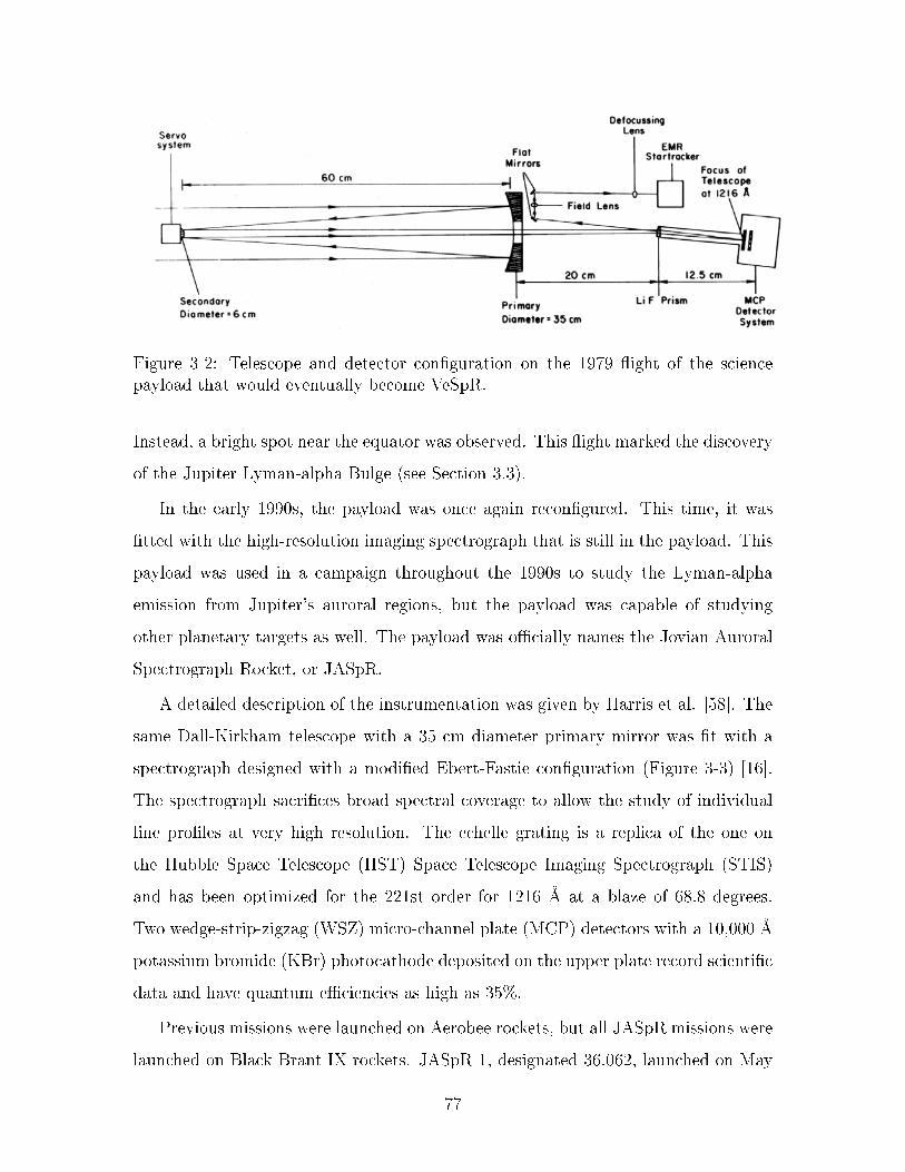
Figure 3-2: Telescope and detector conguration on the 1979 ight of the sciencepayload that would eventually become VeSpR.
Instead, a bright spot near the equator was observed. This ight marked the discovery
of the Jupiter Lyman-alpha Bulge (see Section 3.3).
In the early 1990s, the payload was once again recongured. This time, it was
tted with the high-resolution imaging spectrograph that is still in the payload. This
payload was used in a campaign throughout the 1990s to study the Lyman-alpha
emission from Jupiter's auroral regions, but the payload was capable of studying
other planetary targets as well. The payload was ocially names the Jovian Auroral
Spectrograph Rocket, or JASpR.
A detailed description of the instrumentation was given by Harris et al. [58]. The
same Dall-Kirkham telescope with a 35 cm diameter primary mirror was t with a
spectrograph designed with a modied Ebert-Fastie conguration (Figure 3-3) [16].
The spectrograph sacrices broad spectral coverage to allow the study of individual
line proles at very high resolution. The echelle grating is a replica of the one on
the Hubble Space Telescope (HST) Space Telescope Imaging Spectrograph (STIS)
and has been optimized for the 221st order for 1216 Å at a blaze of 68.8 degrees.
Two wedge-strip-zigzag (WSZ) micro-channel plate (MCP) detectors with a 10,000 Å
potassium bromide (KBr) photocathode deposited on the upper plate record scientic
data and have quantum eciencies as high as 35%.
Previous missions were launched on Aerobee rockets, but all JASpR missions were
launched on Black Brant IX rockets. JASpR 1, designated 36.062, launched on May
77
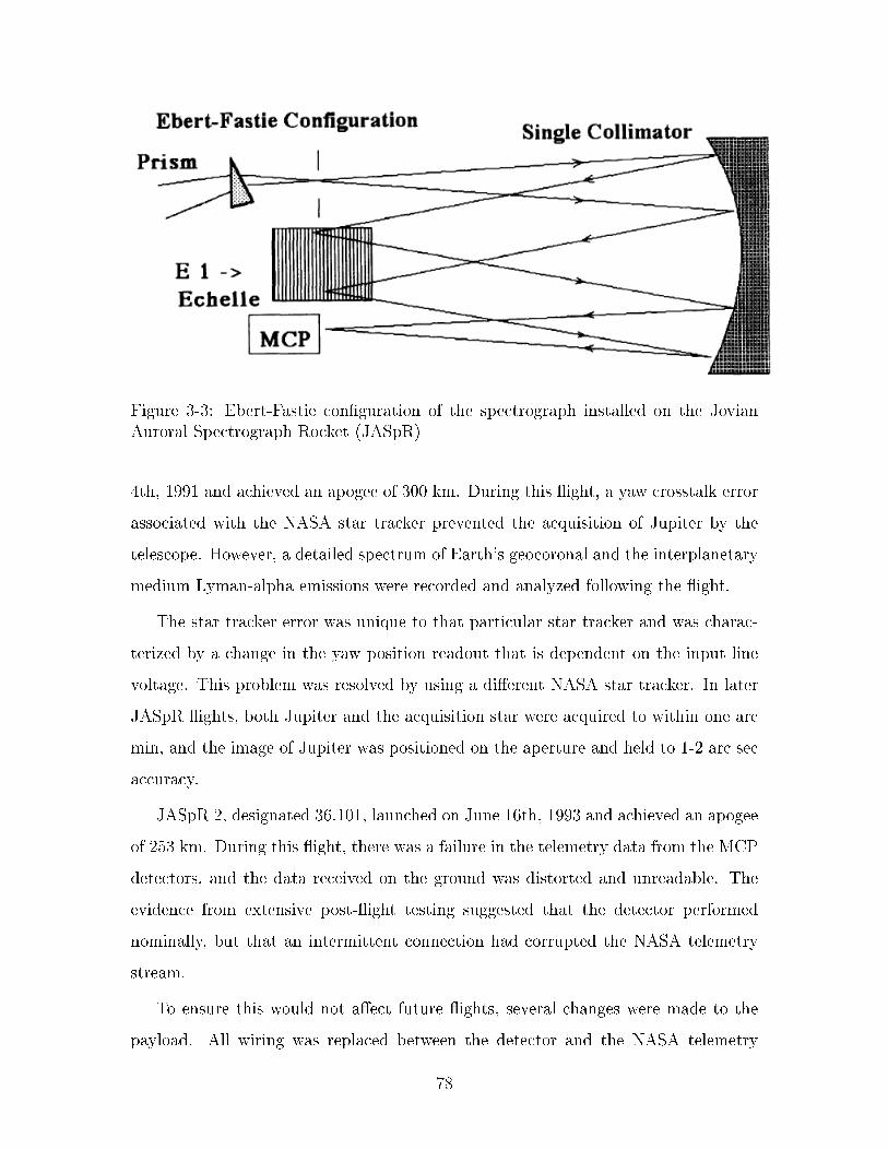
Figure 3-3: Ebert-Fastie conguration of the spectrograph installed on the JovianAuroral Spectrograph Rocket (JASpR)
4th, 1991 and achieved an apogee of 300 km. During this ight, a yaw crosstalk error
associated with the NASA star tracker prevented the acquisition of Jupiter by the
telescope. However, a detailed spectrum of Earth's geocoronal and the interplanetary
medium Lyman-alpha emissions were recorded and analyzed following the ight.
The star tracker error was unique to that particular star tracker and was charac-
terized by a change in the yaw position readout that is dependent on the input line
voltage. This problem was resolved by using a dierent NASA star tracker. In later
JASpR ights, both Jupiter and the acquisition star were acquired to within one arc
min, and the image of Jupiter was positioned on the aperture and held to 1-2 arc sec
accuracy.
JASpR 2, designated 36.101, launched on June 16th, 1993 and achieved an apogee
of 253 km. During this ight, there was a failure in the telemetry data from the MCP
detectors, and the data received on the ground was distorted and unreadable. The
evidence from extensive post-ight testing suggested that the detector performed
nominally, but that an intermittent connection had corrupted the NASA telemetry
stream.
To ensure this would not aect future ights, several changes were made to the
payload. All wiring was replaced between the detector and the NASA telemetry
78

encoder to ensure solid electrical connections. A backup ight data recorder was
added to store MCP data directly from the detector so it could be recovered after
ight if there was a failure in the telemetry data received on the ground. Finally, the
MCP detectors were replaced with newer, higher-resolution detectors and associated
signal processing electronics.
JASpR 3, designated 36.104, launched on April 1st, 1995 and achieved an apogee
of 253 km. During this ight, the telemetry recorded a high voltage discharge on
the MCP detector. This was later traced to a Reynolds 600 series connector that
provides high voltage to the detector housing that had not been properly cleaned
and tightened before ight. Protocol was introduced where the Principal Investigator
inspects and attaches all high voltage connectors before ight.
JASpR 4, designated 36.149, launched on October 29th, 1996 and achieved an
apogee of 300 km. During this ight, none of the previously encountered problems
were present, but the overall count rate recorded by the MCP detectors was signi-
cantly lower than necessary to meet the science goals of the mission. This was likely
due to contamination of the optics during the extensive high vacuum testing the
payload underwent before ight to demonstrate that there would be no high voltage
arcing on either detector at any pressure. The vacuum chamber used diusion pumps
to achieve vacuum, and there is evidence that diusion pump oil entered the chamber
and contaminated the optics.
This contamination would have been discovered had the payload gone through an
additional absolute calibration before the ight. Unfortunately, the testing chamber
at the University of Colorado that was used to show the optics were in alignment
did not have the ability to perform an absolute calibration of the whole system. In
response, the Vacuum Calibration and Testing Facility (VACTEF) was designed and
built to perform clean, high vacuum payload calibration and testing for future ights.
The optics were recoated to achieve higher eciency on later ights.
JASpR 5, designated 36.174, was never launched due to budget cuts in the sound-
ing rocket program. In addition, there was a failure of the data stream during testing.
Data from the spectrograph detector stopped coming through the ground support sys-
79

tem, and because the program had been canceled, the exact cause of this problem
was never discovered. Furthermore, one of the servos on the secondary mirror that
controlled the tip/tilt had burned out, so the mirror was only able to adjust itself in
one direction during ight. The payload was put in to storage in 2003 with constant
power to the VIPs to hold the detectors at vacuum until they were used again.
3.2 Previous Measurements of the Deuterium/Hydrogen
Ratio on Venus
VeSpR will not be the rst mission to study the water history on Venus. Several
other missions have attempted to understand the elevated D/H ratio that has been
measured on the planet, but none have been able to unambiguously constrain the D/H
ratio above the homopause. Other missions have measured HDO/H2O with signicant
accuracy at lower altitudes; however, in order to understand atmospheric escape of
hydrogen and the photodissociation of water in planetary atmospheres, the D/H ratio
above the altitude where photodissociation occurs must be better understood. This
section reviews some of the previous work that has attempted to measure the D/H
ratio or the HDO/H2O atmosphere in various areas of the Venus atmosphere.
3.2.1 Mariner 5 (1967)
Mariner 5 was launched on June 14th, 1967 and ew by Venus on October 19th of that
year. Among its scientic instruments was an ultraviolet photometer that measured
ultraviolet light through three lters. The eective passbands for the three channels
were 1050 to 2200 Å, 1250 to 2200 Å, and 1350 to 2200 Å [10]. The dierence between
the signals observed by the rst two channels was the Lyman-alpha emission from
atomic hydrogen. The results initially implied that the temperature several hundred
kilometers above the surface was much lower than the temperature at comparable
altitudes on Earth; this would imply that the escape rate of atomic hydrogen by
Jean's escape was also much lower than on Earth.
80

Further analysis of this data showed that these Lyman-alpha measurements could
only be t with barometric-exospheric equations if a two-component model of the
atmosphere was used [5]. Three possible hypotheses for these two components were
proposed. The rst was that there was an abundance of molecular (H2) molecules
in addition to atomic hydrogen in the upper atmosphere. This atomic-molecular
hydrogen model was initially considered the most realistic explanation for the Mariner
V Lyman-alpha data. The second was a two-temperature model, but this model would
require two separate sources of hydrogen. The third model was a deuterium-hydrogen
model. This model was not preferred over the atomic and molecular hydrogen model
because it required a D/H ratio of 10 or higher.
The deuterium-hydrogen model was later re-examined. It was shown that the D/H
ratio of 10 predicted by Barth [5] could be reconciled with transport and diusion
mechanisms. McElroy and Hunten [44] showed that the D/H ratio could be 0.1, which
is still an enhancement of several orders of magnitude compared to the terrestrial value
of 1.6 x 10⁻⁴. Their work was the rst to conclude that an elevated D/H ratio was a
serious possibility.
3.2.2 Pioneer Venus (1978)
The Pioneer Venus mission was a two-vehicle combination of an orbiter and a multi-
probe launched by NASA. The multiprobe consisted of a bus that carried one large
and three small probes that all entered Venus' atmosphere on December 9th, 1978
[37]. The large probe's neutral mass spectrometer (LNMS) entered near the equator
and measured the abundances of atmospheric constituents as it descended into the
Venus atmosphere, slowed by a parachute [24].
At an altitude of 64 km, two microleak channels on the instrument allowed gas
from the atmosphere into the spectrometer [53]. The instrument scanned the mass
spectrum from 1 to 208 atomic mass units once every 64 seconds.
There is debate about the validity of the data from the LNMS. The instrument was
backlled with helium and nitrogen during its voyage to Venus. There is evidence
that it was also contaminated with terrestrial moisture, and that moisture had a
81

Figure 3-4: Ratio of counting rates of HDO/H2O as a function of data frame takenfrom Donahue et al. [53]. The horizontal axis indicates the frame number of the data(bottom scale) and altitude in km (top scale). The vertical axis indicates the D/Hratio. The data between the two vertical lines indicate the time when the spectrometerinlet was clogged with droplets of sulfuric acid.
terrestrial value for the HDO/H2O ratio. The inlet tubes were heated to prevent con-
densation, which would have produced terrestrial water vapor that the spectrometer
then measured.
When the large probe descended beneath 50 km, the spectrometer microleak chan-
nels clogged with sulfuric acid, most likely from cloud droplets. One of the microleak
channels was shut o at 47 km and the other cleared between 29 and 26 km. Donahue
et al. argue that the best measurements of the HDO/H2O ratio come when the inlet
is clogged with Cytherean droplets. When this happened, the count rate dramati-
cally increased and with it the signal-to-noise ratio of the data. Figure 3-4 shows the
ratio of HDO/H2O calculated from the raw data as a function of frame number and
altitude.
The analysis from the LNMS data shows that the D/H ratio within this altitude
82

range in the atmosphere is 1.6 x 10⁻². This agrees with the ratio of 10-2 found by
McElroy et al. [45] using the same spectrometer data, who argue that the ion with a
mass of 2 atomic mass units found by LNMS was ionized deuterium and not hydrogen
molecules (which also have a mass of 2 atomic mass units). Donahue et al. further
argue that this hundred-fold increase in the D/H ratio compared to Earth's D/H ratio
sets a lower limit of 0.3% of a terrestrial ocean of water has escaped from Venus (see
Section 2.2).
It was later shown that the densities of hydrogen and deuterium in the nightside
thermosphere varied with the Solar cycle [47]. In-situ measurements made using the
Pioneer Venus Orbiter Ion Mass Spectrometer (OIMS) during its pre-entry phase
when the Solar cycle was close to Solar minimum show enhancements in hydrogen of
6.5 times and deuterium of 4 times compared to later years when the Solar cycle was
at Solar maximum. This showed that the buildup during Solar minimum is caused
by a reduction in the escape uxes of hydrogen and deuterium.
However, these in-situ measurements were only taken above 170 km, which is
several scale heights above the lower boundary where carbon dioxide absorption of
Lyman-alpha decreases the photodissociation rates of H2O and HDO. In addition, the
spectrometer did not measure deuterium directly, only the ions with a mass of two.
This measurement could correspond to molecular hydrogen in those regions as well
as deuterium even though it has been shown that the molecular hydrogen density is
low.
3.2.3 Telescopic Observations of Venus
In 1980, the International Ultraviolet Explorer (IUE) observed Venus while the planet
was at maximum elongation and recorded a series of spectra with a total observation
time of 260 minutes. The goal was to measure deuterium in the upper atmosphere
above where Pioneer Venus' LNMS measured HDO/H2O. Figure 3-5 shows the data
from the combination of the spectra taken from [27]. These results show Venus' hy-
drogen Lyman-alpha emission to be 21±5 kR, which is consistent with measurements
from Pioneer Venus.
83

Figure 3-5: Hydrogen Lyman-alpha emission of Venus measured by the InternationalUltraviolet Explorer (IUE) taken from Bertaux and Clarke [27]. The solid line cor-responds to the observed data, a 21 kR emission. The dashed line corresponds tothe prole calculated for a 2.5 kR deuterium emission, expected for the D/H ratiomeasured by Pioneer Venus of 1.6 x 10⁻². The Net Flux units (a.u.) denote 105 IUEux units.
However, the results do not show evidence of a deuterium emission, which was
expected to be on the order of 2.5 kR based on the deuterium abundance found by
Pioneer Venus. Instead, the IUE observations only placed an upper limit of 300 R
on the deuterium emission, which Bertaux and Clarke argued corresponds to a D/H
ratio of 2 x 10⁻³, a factor of 8 less than the Pioneer Venus measurement.
In view of this discrepancy, Bergh et al. used the Fourier Transform Spectrometer
with the 3.6 m Canada-France-Hawaii telescope on Mauna Kea to detect HDO and
H2O in Venus' atmosphere in an altitude range between 32 and 42 km [9]. Their
spectral observations in the 3-4 µm range found total abundances of H2O and HDO
to be 34±10 and 1.3±0.2 parts per million, corresponding to a D/H ratio of 1.9±0.6
x 10-2, which is consistent with what was measured by Pioneer Venus. However, these
results still do not directly measure D/H in the upper atmosphere.
84

3.2.4 Venus Express (2007)
The European Space Agency (ESA) launched Venus Express on November 9th, 2005.
It was the agency's rst mission to Venus. The spacecraft is very similar to the
successful Mars Express launched two and a half years earlier, but its design was
modied to withstand the more severe thermal environment [14]. It carries seven
suites of science instruments to study Venus; ve were inherited from the Mars Express
and Rosetta missions with slight design modications, and two instruments were
specially designed for Venus Express.
The Spectroscopy for the Investigation of the Characteristics of the Atmosphere of
Venus (SPICAV) is one of the suites that was borrowed from Mars Express. SPICAV
is a suite of three spectrometers, one in the ultraviolet wavelength range and two in
the infrared wavelength range. The goal of the experiment is to study the composition
and structure of Venus' upper atmosphere [14, 28].
The ultraviolet spectrometer is identical to the one own on Mars Express [14]. It
operates within the 110-320 nm wavelength range with a resolution of 1.5 nm. This
instrument does not have the resolution to directly detect the separate Lyman-alpha
emissions from deuterium and hydrogen atoms. It was speculated that the combined
intensity prole could be separated with data from this instrument by examining
the variation with altitude [28]. The optically thick hydrogen emission should vary
smoothly with altitude down to where carbon dioxide absorption dims the emissions
(near 120 km), while the optically thin deuterium emission would cause a spike above
this altitude. However, this technique was not successful in determining the D/H
ratio in the upper atmosphere.
One of the other SPICAV instruments is the Solar Occultation Infrared (SOIR)
spectrometer. The SOIR spectrometer operates within the 2.2-4.4 µm range and was
designed and developed specially for Venus Express [14]. It has a resolving power of
15,000-20,000, which is enough to resolve the H2O and HDO absorption proles in a
stellar occultation.
Between December 21st, 2006 and January 8th, 2007, SOIR measured the abun-
85

Figure 3-6: Data from Venus Express' SOIR measuring (left) abundance of HDO andH2O and (right) the HDO/H2O ratio [29]. The measurements on Orbits 244, 251,and 262 were taken at latitudes of +85, 83, and 73 degrees. Error bars indicate 1standard deviation.
dance of HDO and H2O in the Venus atmosphere between 70 and 110 km altitude
at high polar latitudes. Figure 3-6 (left) shows the vertical mixing ratios of each
molecule and Figure 3-6 (right) shows the ratio of the two abundances [29]. These
measurements show little temporal variation. At the lower altitude boundary, the
HDO/H2O mixing ratio is close to 0.1 with an error bar (1 standard deviation) over
50%. This is within the bounds of what has been measured in the bulk atmosphere
at lower altitudes [53, 45].
The mixing ratio was expected to decrease with altitude because of the preferential
condensation of HDO [26], but it instead increases up to 0.12, which is about 2.5 times
the HDO/H2O ratio in the bulk atmosphere. This suggests that there is no cold trap
preventing photodissociation in the upper atmosphere, and that the increase in the
ratio is due to the lower photodissociation rate of HDO compared to H2O. Laboratory
tests have shown that HDO has a lower ultraviolet cross-section than H2O at Lyman-
alpha, so it is dissociated by photons at a lower rate [6].
86

The higher HDO/H2O ratio at higher altitudes could also mean hydrogen atoms
are escaping into space much faster than deuterium atoms, which are left behind
and recombine with OH radicals [29]. This would be the rst measurement of hy-
drogen escaping more quickly than deuterium, and the presence of deuterium atoms
in the photodissociation region indicates deuterium is present in the thermosphere.
Quantifying the deuterium and its ratio to hydrogen above this region is essential for
understanding the escape mechanisms.
Since the UV spectrometer was unable to measure the D/H ratio in the upper
atmosphere directly, this measurement is still missing. The Venus Spectral Rocket
Project was proposed specically to complement the SOIR data to better understand
the photodissociation and escape mechanisms and rates. VeSpR will measure the
Lyman-alpha ux of deuterium and hydrogen above 110 km.
3.3 Previous Observations of the Jupiter Lyman-alpha
Bulge
Over the past three decades, there have been a number of space missions to send
probes and orbiters to Jupiter. Those missions, along with additional telescopic
observations from both ground-based and space telescopes, have greatly broadened
our understanding of Jupiter, its atmosphere, its aurorae, and its magnetosphere.
However, the upper atmospheric asymmetry known as the Lyman-alpha Bulge still
cannot be explained entirely. The leading hypotheses for the source of this energy
are summarized in Section 2.4 while the Bulge observations are summarized here.
The Lyman-alpha Bulge was rst discovered by a sounding rocket experiment
(see Section 3.1) own on December 1, 1978. The experiment measured the spatial
distribution of Lyman-alpha ux on the planetary disk and found an average disk
brightness of 13 kR. There was an area on the disk with brightness a few kR higher
than the average at 80 degrees System III longitude near the equator [32]. Figure 3-7
shows the data from the experiment.
87

Figure 3-7: Contour plot of the brightness of Jupiter during the rocket observation[32] (color added for clarity). Brightness is in units of kR. The small bright spotwhere 19 kR is marked is the sub-Solar point, and the larger bright spot is the Bulge.
Additional observations from the ultraviolet spectrometers aboard Voyager 1 and
Voyager 2 soon followed in early 1979 [1, 3]. These observations also showed a strongly
asymmetry in Lyman-alpha brightness along the equator. A minimum brightness of
14.4 kR was observed around the entire planet with a broad peak at 19.6 kR near a
longitude of 110 degrees in the System III magnetic coordinate system, corresponding
to a 36% increase in brightness [4].
More observations of the bright region were made using the International Ultra-
violet Explorer (IUE) in May-June 1979 and May-July 1980 as follow ups to the
sounding rocket experiment. [33]. Spatial imaging was achieved with IUE's short-
wavelength spectrograph. The study showed a peak between 50 and 100 degrees in
the System III coordinate system and a 20% decrease in brightness from one year to
the next even as the brightness along the rest of the disk stayed constant.
A number of explanations for this asymmetry were proposed. The Voyager data
authors suggested that the emission represented an increased column density due
to dissociation of H2 molecules by hot plasma in the inner magnetosphere [4]. The
emission bulge at Lyman-alpha is then due to increased resonant scattering because
of this higher column density. Using the radiative transfer model in [32], this would
88

require a column of hydrogen atoms over 50% more dense compared to the rest of the
planet, which is why it was named the Jupiter Lyman-alpha Bulge.
From 1982 to 1988, the IUE observed a series of spectra of the auroral regions of
Jupiter. These observations showed that roughly ÷ of the Lyman-alpha emission from
the auroral regions were blue-shifted by 30-60 km/s [30]. This is a signicant fraction
of the escape speed of Jupiter and is evidence of a large outow of hydrogen ions
and atoms owing outward into the Jovian magnetosphere from the auroral regions.
Although IUE did not observe the Bulge directly, high-velocity hydrogen from the
auroral regions may have a signicant eect on the Bulge.
An additional long-term observation campaign of Jupiter was conducted from
1978 to 1989 with IUE, this time focusing on variations in the Jovian H2 dayglow
emission over time. The study spans the decline in Solar activity from the end of Solar
cycle 21 to the rise in Solar activity from the beginning of Solar cycle 22 [41]. This
study found no other long-term asymmetrical molecular hydrogen emission feature
on Jupiter analogous to the Lyman-alpha Bulge, conrming another nding from
Voyager [4].
During this long-term study, spectra were obtained of the equatorial region show-
ing the change in brightness as a function of time and longitude. Figure 3-8 shows
the average Lyman-alpha emission brightness from 1985 to 1989 plotted against the
System III longitude. This data shows brightening in the longitudinal areas predicted
by previous Bulge observations, although the bin size for the averages plotted is not
ne enough to constrain the longitude of the Bulge to within ±5 degree. While the
error bars shown in the gure are a signicant fraction of the data, it does show
evidence that the brightness of the Bulge varies over time with the Solar cycle.
Further observations of the Bulge were conducted with IUE's short wavelength
prime (SWP) echelle spectrograph from February 1990 to April 1991 [31]. This data
showed that the Lyman-alpha emission line prole is signicantly broader than the
0.14 Å spectral resolution of the instrument at all longitudes, the equatorial emission
lines are broader than the mid-latitude emission lines, and Bulge emission lines are
broader than the emission lines from other areas of the equatorial region. Line-
89

Figure 3-8: Lyman-alpha emission of Jupiter with respect to longitude in System IIIshowing the overall rise in brightness from 1985 to 1989 [41]
broadening eects, such as broadening by collisions and the Stark eect, are ineective
by several orders of magnitude for explaining this result. The line broadening was
explained by the presence of superthermal hydrogen atoms in the upper atmosphere,
which resonantly scatter the broad solar emission line.
Ben Jael et al [40] proposed that this superthermal population could be accounted
for with a two-component turbulent model where a fraction of the atomic hydrogen
moved in a non-thermal velocity eld. The best t of this model to the IUE data
from [31] was when the total hydrogen column density is 3.7 x 1017 cm-2 with a
non-thermal component density of less than one percent of the total density and a
turbulent velocity of 9 km/s (Figure 3-9). An explanation involving turbulence is not
necessary to model the spectra at mid-latitudes because an existing radiative transfer
model t the data well [38].
This model ts the data well and is consistent with other characteristics of the
Bulge, such as its existence on the night side of the planet, and it could explain the
excess heating in the atmosphere. However, a source of energy is required to drive
a turbulent process that would generate the eects shown in the data. A number
of explanations have been proposed (Section 2.4) but none have been shown with
observations to account for the energy transfer to the Bulge region without requiring
90

Figure 3-9: IUE spectrum of the Bulge on the limb from [31] shown with model proleswith and without turbulence[40]. The best t of the turbulent model is obtained witha hydrogen column density of 3.7 x 1017 cm-2 and a turbulent velocity of 9 km/s.
other phenomena that have been shown to not be present.
Observations with the Hubble Space Telescope (HST) Goddard High-Resolution
Spectrograph (GHRS) in May 1994 revealed more broadening and brightness of the
line core of Bulge spectra compared to the Anti-bulge and mid-latitude spectra [11].
These results conrmed that the Lyman-alpha Bulge is associated with hydrogen line
broadening rather than an enhancement of the brightness near the line center, which
ruled out the excitation of the Bulge by electron impact on ambient hydrogen atoms
that was suggested as part of the electroglow processes.
The GHRS data also showed evidence of supersonic turbulence. When turbulent
hydrogen cells are modeled as a two-component Gaussian distribution (shown in Fig-
ure 3-10), the best t to the data is when hydrogen cells moved a 5 km/s with a
standard deviation of 40 km/s. This corresponds to a hydrogen escape rate of ~1029
atoms per second over the Bulge region. Additionally, Ben Jael et al. [40] argued
that the origin of this velocity eld may be related to the Jovian aurora given the
supersonic Doppler-shift in the auroral Lyman-alpha emission and the high energy
injected into the planets at high latitudes from magnetic particles because the Bulge
and the aurorae are both xed with respect to the magnetic eld.
Further spectral observations of Jupiter with GHRS occurred in June 1994. This
campaign observed Lyman-alpha spectra of the auroral regions. This study's primary
91

Figure 3-10: Turbulent model and data from Emerich et al. [11]. The turbulentmodel is colored in red here for clarity. The two peaks in the model come fromdual-Gaussian model with line centers shifted corresponding to ±5 km/s.
result was evidence of a core reversal in the Lyman-alpha line prole, which was
predicted by models as a consequence of radiative eects on photons produced deep
within the auroral region. This core reversal had never been observed before [48].
However, the secondary result was that the line proles of the auroral spectra
were asymmetric. This could be due to Doppler motions of large masses moving at a
few kilometers per second or by a smaller, more Doppler-shifted component owing
at 20 km/s. If the latter case is true, then this small hydrogen component could be
making its way down toward the equator. If it is moving asymmetrically with the
pole of rotation, this hydrogen could be preferentially streaming into the Bulge region
compared with the rest of the equatorial region.
Observations made in August 1997 from the NASA Infrared Telescope Facility
(IRTF) on Mauna Kea, Hawaii conrm near-supersonic speeds of hydrogen in the
auroral region [15]. These winds were measured to be on the order of 3 km/s. This
conrms the auroral electrojet that could be causing turbulence in the Bulge and
shows its velocity. Figure 3-11 shows the electrojet from a System 3 longitude of 263
degrees, which approximately 150 degrees away from the Bulge. The electrojet wraps
around the planet following a model of the magnetic footprint but there has been
92

Figure 3-11: Infrared ltered image (3.953 µm) of the Jovian north pole showing theauroral electrojet [15]. The red lines show the magnetic footprint from a recent Jovianmagnetic eld model. The latitude lines are separated by 10 degrees, the longitudelines are separated by 18 degrees, and the scale on the sides of the gure are in arcsecs.
no evidence presented yet that these jets make their way all the way down to the
equatorial region.
In late 1997, the Galileo Ultraviolet Spectrometer (UVS) made additional mea-
surements of the Lyman-alpha Bulge and further constrained properties of the hy-
drogen corona. These observations are best t to models when a small amount of
hot hydrogen is included, providing even more evidence for the two-component model
proposed in [40]. The authors concluded that further long-slit echelle observations
of the Bulge to examine the spatial structure would help identify the source of the
energy causing the brightness in the Bulge.
An HST Space Telescope Imaging Spectrograph (STIS) campaign in 1999 and 2001
did just that. High-resolution, long-slit echelle spectra were observed at the Bulge,
Anti-bulge, and latitudes to the north and south of the Bulge while the targets were on
the limb of the planet. These spectra exhibited asymmetries relative to line center,
showing that the red-shifted wings of the broad line prole were more prominent
than the blue-shifted wings [12, 13]. The observed asymmetries were interpreted as
the signature of hot hydrogen atoms propagating in the upper Jovian atmosphere,
with a velocity distribution in excess of the planetary rotation speed.
These high-resolution STIS spectra were used in the development of a parametric
radiative transfer model [39]. This model takes into account frequency redistribu-
tion, phase angle eect, the eect of hydrogen column density, eddy diusion, and
suprathermal hydrogen components to produce spectral line proles of Jupiter's at-
93

mosphere. While this model is not yet complete, preliminary results have shown the
strength of the model as it gets closer to being ready for widespread use. Further
analysis of the STIS spectra can help constrain parameters of the model to more
accurately predict spectral line proles for future observations.
94

Chapter 4
The Venus Spectral Rocket
4.1 VeSpR Flight Prole
In December 2008, the science team and the WFF engineers conducted a Design
Review, the rst of many reviews before launch. This section outlines the payload
hardware, mission timeline, mission success criteria, and the simulated analysis of the
ight as generated by the WFF engineers for the VeSpR payload's ight.
4.1.1 Flight Conguration
The Venus Spectral Rocket consists of three major components, the Terrier booster,
the Black Brant IX booster, and the payload section. The entire rocket is 17.03 m
long. The complete ight conguration is shown in Figure4-1.
The Terrier Mk70 booster is a surplus missile originally designed for military pay-
loads, but has since been modied as a rst stage for suborbital rockets carrying heavy
science payloads like VeSpR. The Black Brant is manufactured by Bristol Aerospace
specically for high-performance suborbital ights.
The payload section is customized for the VeSpR ight, although some equipment
is used for other suborbital ights, and standard spacecraft buses are used where
appropriate. The payload team at Boston University is responsible for the science
experiment, which consists of the six sections from left to right labeled Spectrom-
95

Figure 4-1: Conguration of the full rocket, consisting of two boosters and the pay-load.
Figure 4-2: Solid model of the payload section conguration.
eter Extension through Telescope Extension in Figure 4-2. A detailed overview of
the experiment can be found in Section 4.2. The remaining payload sections are the
responsibility of engineers at WFF and will be briey discussed here, but more in-
formation regarding these sections is available the Design Review Documents (4.0
Mechanical Engineering Package) in the attached Appendix DVD.
At the top of the rocket is the nosecone, formally called the Ogive Recovery System
Assembly (ORSA), which houses the parachutes used to recover the payload. It also
contains a set of pitch nozzles used in conjunction with a second set located in the
next section, the Linear Thrust Module (LTM). The LTM provides for ne pointing
capability of the payload and contains a set of pitch nozzles, an LN-251 gyro, and
associated electronics and plumbing. Figure 4-3 shows the 1000 lb ORSA, and Figure
4-4 shows the LTM.
The next section is the Celestial Attitude Control System (CACS) and it provides
the pointing capability of the payload. It houses the electronics control of the ST-5000
96

Figure 4-3: 1000 lb ORSA Assembly
Figure 4-4: Linear Thrust Module (LTM)
97

Figure 4-5: Celestial Attitude Control System (CACS)
star tracker, a Gimbaled LN-200 with a Miniature Airborne Computer (GLNMAC)
internal measurement unit (IMU), a gas tank, and various associated regulators,
plumbing, and electronics. The Piggy Back Tank (PBT) assembly houses two 200 in3
gas tanks for additional attitude control and pointing along with associated plumbing.
The additional gas may be necessary because of the number of targets that VeSpR
needs to acquire for mission success and if the ST-5000 star tracker has trouble locking
on to Venus (see Sections 4.1.2, 4.1.3, and 5.1.3). Figure 4-5 shows the CACS, and
Figure 4-6 shows the PBT assembly.
The next section down from the nosecone is the S-19L, a guidance system devel-
oped by RUAG Space that functions for the rst 18 seconds of ight, actively guiding
the vehicle by moving four gimbaled canards. The canards are controlled by a pneu-
matic system and are decoupled after 18 seconds using a pyrotechnic device. The
S-19L is a standard system for suborbital rockets, and it is shown in Figure 4-7.
The nal section of the payload before reaching the experiment section is the
Telemetry (TM) section. This section is completely customized for VeSpR and con-
tains all of the antennas used to communicate with the ground. This section of the
payload houses the WFF-93 Pulse Code Modulator (PCM), an electronic device that
houses multiple decks to receive inputs from a variety of dierent signals sources and
types and transmits data to the antennae. Certain details about the TM system are
98

Figure 4-6: Piggy Back Tank (PBT) assembly
Figure 4-7: S-19L guidance system
99

Figure 4-8: Telemetry (TM) section.
not published due to International Trac in Arms Regulations (ITAR) restrictions.
Figure 4-8 shows the TM section.
Next in the payload conguration is the experiment section. The experiment
houses a telescope, optics, MCP detectors, a Xybion camera, a SPACOM star tracker,
and various other electronics including power transformation and monitoring. The
two primary science instruments are the MCP detectors, one attached to a spectro-
graph and one attached to an ultraviolet reimaging box. A more thorough overview
of the payload is presented in Section 4.2.
After the experiment section, the remainder of the non-science payload is attached
to the end of the telescope with the Shutter Adapter and the Ballast Ring. Figure 4-9
shows these two parts. After these adapters is the Shutter Door. The Shutter Door
only serves as a dust door because the science payload does not need to be in vacuum,
so it does not have a vacuum seal. The Shutter Door opens when the payload is above
110 km and closes before the payload descends beneath that altitude. Figure 4-10
shows the Shutter Door.
100

Figure 4-9: Shutter Adapter (left) and Ballast Ring (right)
Figure 4-10: Shutter Door
101
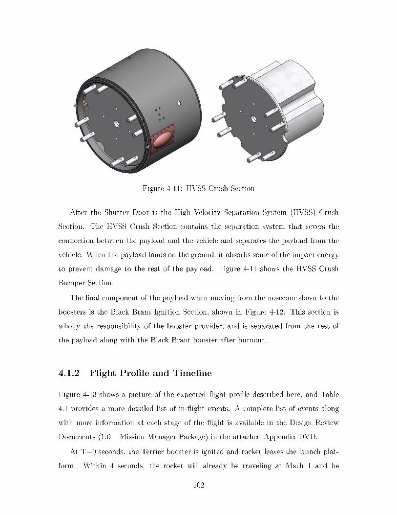
Figure 4-11: HVSS Crush Section
After the Shutter Door is the High Velocity Separation System (HVSS) Crush
Section. The HVSS Crush Section contains the separation system that severs the
connection between the payload and the vehicle and separates the payload from the
vehicle. When the payload lands on the ground, it absorbs some of the impact energy
to prevent damage to the rest of the payload. Figure 4-11 shows the HVSS Crush
Bumper Section.
The nal component of the payload when moving from the nosecone down to the
boosters is the Black Brant Ignition Section, shown in Figure 4-12. This section is
wholly the responsibility of the booster provider, and is separated from the rest of
the payload along with the Black Brant booster after burnout.
4.1.2 Flight Prole and Timeline
Figure 4-13 shows a picture of the expected ight prole described here, and Table
4.1 provides a more detailed list of in-ight events. A complete list of events along
with more information at each stage of the ight is available in the Design Review
Documents (1.0 Mission Manager Package) in the attached Appendix DVD.
At T+0 seconds, the Terrier booster is ignited and rocket leaves the launch plat-
form. Within 4 seconds, the rocket will already be traveling at Mach 1 and be
102

Figure 4-12: Black Brant Ignition Section
Figure 4-13: Pictorial timeline of major events
103

Event Time (s)
Terrier Burnout 6.2Black Brant Ignition 12.0
S-19L Canard Decouple 18.0Black Brant Burnout 44.5
Despin 60.0Payload Separation/ACS Start 64.0
Nosecone Eject 68.0Experiment Video On 72.0Shutter Door Open 75.0
110 km Upleg 75.9Experiment HV On 80.0Settle on Arcturus 99.0
Begin Maneuver to 6 Virginis 124.0Settle on 6 Virginis 148.0
Begin Maneuver to Venus 160.0Settle on Venus 176.0
Apogee 281.4Uplink to Moon 450.0Settle on Moon 477.0100 km Downleg 486.9
Shutter Door Close 490.0300k ft Downleg 496.6
Experiment Video O 500.0Experiment O 500.0ACS Spin-up 500.0ACS Vent 520.0
ACS Valves O 565.0Ballistics Impact 574.8Chute Deploy 633.2
ACS O 700.0Payload Impact 885.7
Table 4.1: List of events on the timeline
104

experiencing more than 10 gs of acceleration (see Section 4.1.4). At T+6.2 seconds,
the Terrier booster will burn out and separate. The rocket will coast for less than
6 seconds before the Black Brant booster is ignited at T+12 seconds. The Blant
Black will burn out at T+44.5 seconds, after which the rocket will be on a ballistic
trajectory.
The Black Brant booster will separate from the payload at T+64 seconds. Since
the telescope is facing down during launch, the payload must ip 180 degrees to point
toward the zenith. The payload begins rotating toward the sky after separation. At
T+75 seconds, the experiment shutter door will open, exposing the star trackers to
the sky as the payload passes the 110 km altitude mark. The payload will begin
maneuvering to its rst target, the star Arcturus, and will be locked onto Arcturus
by T+99 seconds. The Lyman-alpha output of Arcturus is very bright compared
to other stars and has been studied extensively, making it an ideal candidate for an
in-ight calibration of the instrumentation in the payload. This calibration will be
crucial for determining the sensitivity of the science instruments and for analyzing
the data from Venus. VeSpR will observe Arcturus for 25 seconds.
At T+124 seconds, the telescope will begin its move to point at a guidance star
that will be determined before launch. The telescope will settle on the star by T+148
seconds. Once a lock has been acquired, VeSpR will begin its maneuver to point at
Venus, and it will lock onto Venus at T+176 seconds. The guidance star is needed as
an intermediate point between Arcturus and Venus because the ST-5000 star tracker
is unable to track planets. The guidance star will be suciently high in the sky such
that the sky background will not be too bright for the star tracker to lock onto the
star but not so far away that guidance uncertainty in the maneuver from the star to
Venus will make it dicult to lock on to Venus (see Section 5.1.3).
While VeSpR is pointed at Venus, apogee will be reached at T+281 seconds. At
T+450 seconds, after 274 seconds of observing the target, VeSpR will begin its ma-
neuver to point at the sunlit Moon and lock on by T+477 seconds. By T+490 seconds,
VeSpR will have fallen down below the 110 km altitude mark, and Lyman-alpha ab-
sorption by Earth's atmosphere will be too high for quality data to be obtained. The
105

shutter door will close and the experiment will be turned o to prepare for landing.
The parachutes will deploy at T+663 seconds, and the payload is expected to impact
the ground at T+885 seconds, almost 15 minutes after launch.
4.1.3 Mission Success Criteria
The timeline in the preceding subsection was generated based on the nominal mission
performance expectations based on mass estimates of the payload and known perfor-
mance characteristics of the boosters. The mission may not go exactly according to
this timeline during ight. It is important that the Principal Investigator and the
Mission Manager both have the same understand for what mission success is.
Writing down and agreeing on these criteria is a crucial top level that many other
mission requirements on which are based. Just like any other NASA mission, VeSpR
had a Requirements Denition Meeting (RDM) to detail the mission expectations
and nalize the Mission Success Criteria (MSC) so all team members working with
all the stakeholders understand what is expected so that lower-level requirements can
be written to drive the design process in the systems engineering of the mission.
Not only is it important to establish MSC so that lower level requirements can
be written, the MSC can also help determine who is ultimately responsible in the
event of a failure. In most cases, the science payload team can take some course of
action if the ight provider fails to perform up to these criteria and may be able to
launch the experiment on another ight. Likewise, the ight providers can also be
absolved of all blame in the event that the Principal Investigator and the science
team have failed to specify the MSC with enough detail to complete the intended
scientic objective. It is in this area, where hard science objectives and experiment
expectations meet engineering requirements that many problems in missions occur.
Having a well-dened set of MSC ensures that both the science team and the ight
provider have the same interpretation of what constitutes a mission success.
The MSC for VeSpR are split into two categories, Comprehensive Success (CS)
criteria and Minimum Success (MS) criteria. In the event that MS is not achieved
during the ight, the experiment team has the option to have a reight free of charge
106

Table 4.2: VeSpR Mission Success Criteria
(assuming the experiment is still intact). However, if MS is achieved but CS is not,
then the experiment team will have to obtain funding for a new mission entirely if
another ight is desired to complete the scientic objective. Table 4.2 lists the Mission
Success Criteria agreed upon for VeSpR following the RDM.
In order for VeSpR to achieve CS, both the calibration star and Venus must
be observed with both MCP detectors for a minimum of 250 seconds. Notice that
observing the Moon is not a requirement for CS. If launch occurs on a date where
the moon is either not in the sky or it is too far away from Venus to be pointed in a
reasonable amount of time, this maneuver can be cancelled and Venus can be observed
for longer. The reason for pointing at the Moon is to obtain a Solar Lyman-alpha
prole that can be used to characterize the Solar Lyman-alpha light that is shining on
Venus. Since there are other ways to obtain a Solar Lyman-alpha prole at the time
of ight, this is not critical to mission success even though it is desired. However,
the calibration star must be observed because an in-ight calibration is crucial to
determine the sensitivity of the two detectors in ight.
The telescope may be observing one target, but the two MCP detectors are record-
ing entirely dierent phenomena. The detector attached to the spectrograph box will
be recording the Lyman-alpha spectrum that will measure the D/H ratio in Venus'
107

atmosphere, which is the primary scientic objective. The detector attached to the
ultraviolet reimaging box will be recording the rst-ever image of Venus' corona, so
even though CS requires both detectors to be operational, MS can be achieved even
if only one of them is operated because valuable scientic data is still obtained.
A long observation time on Venus is desired because more time on the target
means a higher signal to noise ratio in the data. With higher signal to noise, the
telescope can determine with less uncertainty the D/H ratio of Venus. Higher signal
to noise is especially important if Venus' deuterium emission is dimmer than expected
(see Section 5.5). For CS, 250 seconds of observation is required on both targets, but
for MS, only 60 seconds of Venus observation is required.
CSC2 is an example of a poorly written success requirement. As it is written,
both the calibration star and Venus must be observed for a total of 250 seconds. A
more properly written requirement would have specied minimum observation times
for both Venus and the calibration star rather than the observation time of the two
combined. Even though both the Principal Investigator and the Mission Manager
agreed on the wording of this criterion during the Requirements Denition Meeting
and signed the Success Criteria document, it would be benecial for the mission if this
was revised. Granted, changes in top-level requirements late in the program usually
lead to many problems and cost and schedule overruns, but considering how little this
top-level requirement will change the mission, it would be wise to update its wording
to reect a more accurate expectation of the mission and the declaration of success.
4.1.4 Expected Flight Performance
Wallops Flight Facility has experience launching sounding rockets using a ight con-
guration very similar to what VeSpR will have. VeSpR's length and mass charac-
teristics fall within WFF's ight experience envelope, shown in Figure 4-14. VeSpR
is not unusually heavy or long compared to many other sounding rocket payloads, so
its performance can be predicted with a great deal of accuracy.
Since time above 110 km (which should be maximized according to the Mission
Success Criteria in Table II in Section 4.1.3) is directly related to the apogee altitude
108

Figure 4-14: Flight experience envelope of the Terrier-Black Brant Mk1 (Mod 2)relative to payload weight in pounds and payload length in inches.
of the payload, it is especially important to have accurate predictions on the ight
prole including maximum altitude. The engineers at WFF have run simulations to
predict the ight performance of VeSpR during ight. The nominal apogee of the
payload is 300 km and the nominal distance from the launch location (range) is
less than 80 km, but due to changes in weather conditions, payload mass, booster
performance degradation, and other factors, this may not be the case.
Gaussian statistics used in the model predict a 2-sigma minimum of the apogee
altitude to be 275 km, meaning there is a 2.5% chance that VeSpR's apogee will be
below this value. In addition, the same 2-sigma maximum range shows there is a 2.5%
chance that VeSpR will land more than 93 km away from the launch site. Figure 4-15
shows the predicted ight altitude with respect to time, and Figure 4-16 shows the
ight altitude with respect to range.
Apogee altitude is a major factor in determining mission success because mission
success is constrained by the time above 110 km, but the ight simulations also
provide a wealth of additional information associated with the ight. More of this
109

Figure 4-15: Expected ight altitude and 2-sigma low with respect to time.
Figure 4-16: Expected ight altitude and 2-sigma long with respect to range.
110

Figure 4-17: Expected acceleration during ight with respect to time.
information is available in the Design Review Documents (3.0 Flight Performance
Package) in the attached Appendix DVD, but some of it will be discussed here.
The acceleration prole of the ight is especially important when designing pay-
load systems or making changes to an existing system. Figure 4-17 shows the accel-
eration the payload will experience with respect to time for the rst minute of ight.
Sudden changes in acceleration pose a greater risk to the structural integrity of the
payload than constant high accelerations.
The maximum expected acceleration is just above 13 g's, during the rst 4 seconds
of ight when the Terrier booster is active. Air resistance and gravity begin to slow
the rocket in the 6 seconds between the Terrier burnout and the Black Brant ignition,
which gives a net negative acceleration during this time. After the Blank Brant is
ignited, the acceleration climbs from approximately 4 g's up to over 8 g's.
This slow increase of acceleration is expected; the booster burns propellant and
loses mass as it accelerates, so if thrust stays constant, acceleration must increase
because of the mass decrease. Thrust also tends to increase because solid propellants
are generally cut with circular grains that expand with time and increase the surface
111

Figure 4-18: Expected velocity during ight with respect to time.
area that is burned at any given time. The rate of change of thrust can be controlled
by carving dierent patterns in the propellant grain.
One reason to have a 6-second delay between the Terrier burnout and the Black
Brant ignition is to decrease the dynamic pressure on the rocket during ascent. Since
dynamic pressure (q = 1/2ρv2) is a function of air density as well as velocity squared,
and air density drops quickly with altitude, a lot of spacecraft scale back power after
achieving some sucient speed to prevent damage from high dynamic pressure. The
Space Shuttle throttles back when it achieves its maximum dynamic pressure, known
as Max Q, and gradually increases thrust beyond this point.
Since solid rocket boosters cannot be throttled, there is simply a delay between
the burnout of the rst stage and the ignition of the second stage. During this
period, the velocity only decreases by approximately 25%, but the dynamic pressure
decreases by more than a factor of 2. Compare Figure 4-18, which shows the velocity
prole during ight with respect to time, with Figure 4-19, which shows the dynamic
pressure during ight with respect to time.
Notice that there are two local maxima in the velocity prole, both after the
112
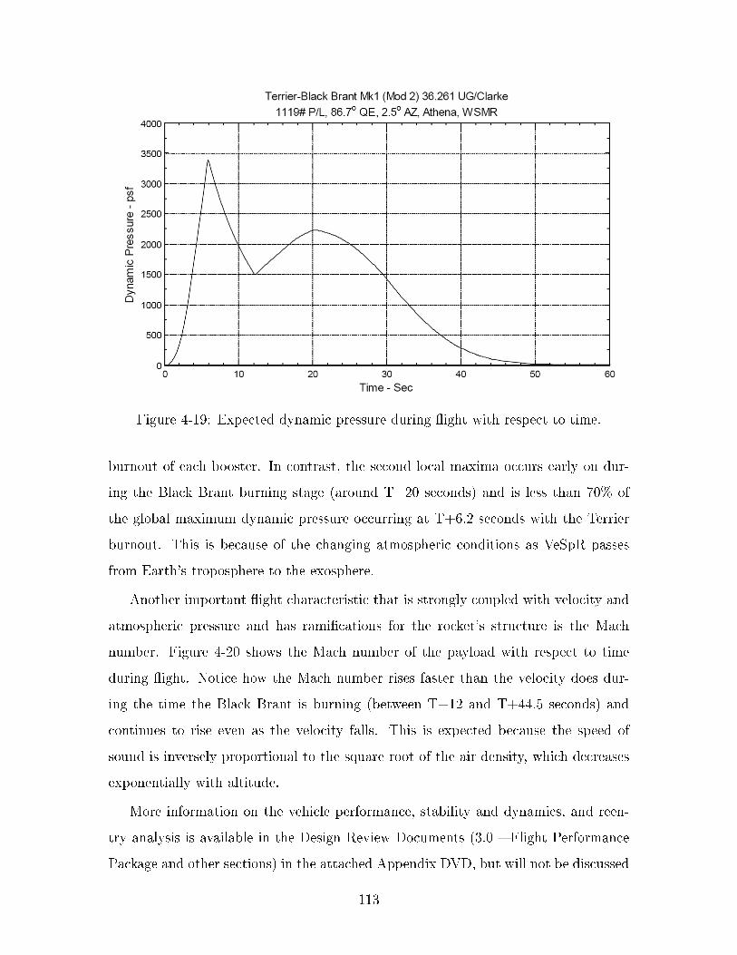
Figure 4-19: Expected dynamic pressure during ight with respect to time.
burnout of each booster. In contrast, the second local maxima occurs early on dur-
ing the Black Brant burning stage (around T+20 seconds) and is less than 70% of
the global maximum dynamic pressure occurring at T+6.2 seconds with the Terrier
burnout. This is because of the changing atmospheric conditions as VeSpR passes
from Earth's troposphere to the exosphere.
Another important ight characteristic that is strongly coupled with velocity and
atmospheric pressure and has ramications for the rocket's structure is the Mach
number. Figure 4-20 shows the Mach number of the payload with respect to time
during ight. Notice how the Mach number rises faster than the velocity does dur-
ing the time the Black Brant is burning (between T+12 and T+44.5 seconds) and
continues to rise even as the velocity falls. This is expected because the speed of
sound is inversely proportional to the square root of the air density, which decreases
exponentially with altitude.
More information on the vehicle performance, stability and dynamics, and reen-
try analysis is available in the Design Review Documents (3.0 Flight Performance
Package and other sections) in the attached Appendix DVD, but will not be discussed
113

Figure 4-20: Expected Mach number during ight with respect to time.
because the author did not perform this analysis himself nor are the details relevant
to the discussion of preparing the scientic payload for ight.
4.2 VeSpR Science Payload Overview
While Wallops Flight Facility and White Sands Missile Range are taking care of the
majority of the rocket and payload support, the science team at Boston University is
preparing the science payload for ight. Here is a detailed description of the major
subsystems in the VeSpR experiment. This section describes the payload as it was
before any additional design changes occurred. Design changes are discussed
in Chapter 5.
4.2.1 Optics Subsystem
The optics in the VeSpR science payload are split into several distinct sections. There
is a telescope, a spectrograph box, an imager box, and a visible optics board. Light
passes through the telescope and an objective prism and hits the spectrograph aper-
114

Figure 4-21: The VeSpR telescope.
ture plate. This aperture plate has a slit that feeds ultraviolet light into the spectro-
graph box, while the remaining light is reected by the plate. The light then reaches
the imager aperture plate; ultraviolet light refracted by the prism passes through a
hole in this aperture plate and enters the imager box, and the remaining light, mostly
visible, enters the visible optics board.
4.2.1.1 The Telescope
The telescope is a Cassegrain design with a Dall-Kirkham gure. It has a 35 cm
diameter ellipsoidal primary mirror and a spherical secondary mirror that provide 1-2
arc sec image quality within a few arc min of the optic axis. The telescope delivers a
f/21 beam to the focal plane with a plate scale of 26 arc sec/mm. A 2-degree mag-
nesium uoride (MgF2) objective prism mounted 48 cm forward of an aperture plate
disperses the converging beam from the telescope, bending the incoming light enough
so that visible and ultraviolet can be separated and directed into their respective
optics. Figure 4-21 shows the VeSpR telescope.
The telescope's secondary mirror is actively controlled by two servomotors that
move pushrods against the back of the mirror. The secondary mirror can be adjusted
to correct for pointing errors of the payload up to 10 arc sec in both pitch and yaw.
Tracking is controlled by a SPACOM star tracker mounted on the visible optics board
115

Figure 4-22: Secondary mirror control servos and pushrods.
that is co-aligned with the telescope. The star tracker has a 4-quadrant photodiode
that produces error signals that are used to drive the servomotors to control the
pointing of the secondary mirror until light from the target object is equal in all four
quadrants. In the last two ights of the telescope, 1-2 arc sec pointing accuracy and
stability was achieved using this compensation scheme, which when convolved with
a telescope image of 1-2 arc sec gives a total point spread function of 2-3 arc sec.
Figure 4-22 shows the secondary mirror control system, disconnected from the back
of the secondary mirror.
One of the servomotors controlling the secondary mirror has burned out, so cor-
rections can only be made in one dimension. This conguration can still work for
the VeSpR mission because the spectrograph aperture slit is so long that the image
of Venus can be aligned to within the pointing accuracy of the entire payload along
the dimension of the inoperable servomotor and still have light from Venus enter the
spectrograph while the other servomotor actively controls the other dimension. How-
ever, this situation is risky and undesirable. The pointing accuracy of the CACS for
the VeSpR payload is ±1.5 arc sec, which is better than the CACSs used in JASpR
missions. Because of this fact and the projected cost to repair or replace the ser-
vomotor assembly, it was decided that this system will be removed for the VeSpR
ight. Now, the error signals from the SPACOM star tracker will be sent directly to
the Telemetry Section to control the ne pointing of the payload (see Section 5.2.3),
116

Figure 4-23: Conguration of the telescope and spectrograph optics.
and a passive system will be used to lock the secondary mirror in place (see Section
5.3.6).
4.2.1.2 The Spectrograph Box
The spectrograph was designed and constructed for UV echelle line prole measure-
ments with long-slit imaging. The Ebert-Fastie conguration employed in the design
of the spectrograph has many characteristics well suited to the science needs of this
mission. The design employs symmetric o-axis reections from a single collimat-
ing mirror to remove aberrations; as a result, the spatial resolution of the system is
limited by the telescope, and the spectral resolution is limited by the grating and
aperture characteristics. Figure 4-23 shows the conguration of the telescope and the
spectrograph box.
The parabolic collimator mirror produces 2 arc sec image quality with minimal
astigmatism along the central 2-3 arc min of the image. The Ebert-Fastie cong-
uration has the additional advantage of being relatively insensitive to the incident
angle of the incoming beam; near parallel to the optic axis, the spectrograph focuses
an image of the aperture at the same location on the detector. This feature greatly
facilitates the alignment process and renders the spectrograph insensitive to small
movements of the collimating mirror that may occur during launch. With the 1216
Angstrom image focused onto the primary aperture, other wavelengths are excluded
from the spectrograph, producing a very low level of scattered light on the detector.
The spectrograph uses a replica of a prototype grating for the STIS, manufactured
117

Figure 4-24: Echelle grating mounted in the spectrograph box and the baes at theentrance and exit of the box.
by the Richardson Grating Lab, which has a 70-degree blaze angle and is optimized
to the 221st order of 1216 Angstrom with a groove spacing of 14.5 µm. For a 5 arc
sec aperture width, the measured resolution in the previous JASpR ight was 0.055
Å FWHM, which is comparable to the expected resolution based on ray tracing with
the BEAM4 program.
The interior surfaces of the housing have been glass beaded to reduce reectivity
to stray UV light. Both the entrance and exit ports are tted with baes, and an
additional bae traps zero order light from the grating. The spectrograph aperture
plate is milled stainless steel with an optical quality front surface, housing a slit
aperture 5 arc sec (190 microns) wide and 390 arc sec (15 mm) long. The 5 arc sec
aperture width is needed for high sensitivity. Figure 4-24 shows the conguration of
the echelle grating and the baes in the spectrograph box.
4.2.1.3 The Imager Box
The imager box was designed and built to re-image the focal plane onto a separate
detector, providing an ultraviolet image of the telescope eld of view minus the light
118

Figure 4-25: Conguration of the telescope and ultraviolet reimaging box optics.
which passes through the spectrograph aperture. The Venus image on the aperture
plate is suciently dispersed by the objective prism that the Lyman-alpha image
will be clearly separated from the longer wavelength continuum and emissions. The
imager box aperture plate is stainless steel with an optical quality nish and an
aluminum/magnesium uoride coating to reect the UV light, and the re-imaging
optics are in the same Ebert-Fastie arrangement as the spectrograph box but with a
at mirror in place of the grating. Figure 4-25 shows the conguration of the telescope
and imager box.
The image scale at the second detector is the same as at the focal plane, and
laboratory tests with a resolution pattern have shown that this system re-images the
focal plane with better than 1 arc sec image quality. In this case, the overall system
resolution is determined by the image quality and target jitter at the focal plane.
Figure 4-26 shows the imager box, and both the spectrograph and the imager box
aperture plates can be seen.
119

Figure 4-26: The imager box and apertures. The black circle with the long horizontalhole is the back of the spectrograph aperture plate, and the mirror with a nearly-circular hole down and to the right is the imager box aperture plate.
4.2.1.4 The Visible Optics Board
The two primary science instruments, the spectrograph and imager boxes and their
detectors, are both imaging ultraviolet light, but visible light entering the telescope
is also observed by additional detectors mounted on the visible optics board. The
visible optics board houses a Xybion camera and a SPACOM star tracker. Figure
4-27 shows the visible optics board.
Visible light enters through the telescope, passes through the objective prism,
reects o both the spectrograph and imager box aperture plates, and passes up
through the large, oval-shaped hole on the visible optics board seen near the top
right in Figure 4-27. The light hits another mirror mounted in the very top right of
the gure that sends the light down through a baed tube. A beam splitter sends
half of the light to the left where it passes through a eld lens, reects o another
mirror, and enters the Xybion camera. The remaining light reects o two additional
mirrors before reaching the SPACOM star tracker.
120

Figure 4-27: Visible optics board. On the left side is the Xybion camera, on the rightis the SPACOM star tracker (gold-colored box).
4.2.2 Detector Subsystem
Two high resolution microchannel plate (MCP) detectors with wedge and strip po-
sitioning anodes and associated electronics were designed and constructed for this
payload. The detectors use four MCPs mounted in a back to back conguration,
each with a gain of 1.2x10⁷ electrons per photon, with a 10,000 Å thick potassium-
bromide (KBr) photocathode deposited on the upper plate. Measurements with a pin
hole mask at the surface of the plates show a resolved pixel of 50 µm, or 1.3 arc sec at
the plate scale of the VeSpR telescope. This provides 2 pixels per 2.6 arc sec resolved
point at the telescope focus. The spectrum is well sampled by the MCP detector,
with 0.011 µm/pixel. The detector readout uses a three electrode wedge and strip
anode 2 cm in diameter. The wedge and strip electrodes employ a linearly variable
surface area to provide 2-dimensional positioning to a high degree of accuracy with
minimum geometric distortion.
The sensitivity of these detectors at Lyman-alpha is 0.15 counts/sec-kR for a 3
121

Figure 4-28: VeSpR MCP detector housing, front view.
arc sec source region. For the Venus ight, Venus' light must be blue-shifted by 0.055
Å or 13 km/sec for the detectors to resolve the hydrogen and deuterium emissions
from the geocoronal emissions in the spectrograph box.
The detectors and their electronics can process up to 10,000 counts/sec, which is
more than adequate for the expected count rate from deuterium in Venus' atmosphere,
before dead time eects create signicant measurement error. The local count rates
on the MCP plates will not induce gain depletion since the counts are spread across
the image of the aperture.
The detector is housed in an evacuated stainless steel housing, and light enters
the housing through a 3.8 cm diameter magnesium uoride window mounted in a
ConFlat ange attached to the front face of the housing. Vacuum is maintained by 2
liter/sec vacuum ion pump (VIP). VIP power is supplied externally by an umbilical
cable and automatically deactivated at launch. On the back of the housing is a plate
with the high voltage input and wedge-strip-zigzag outputs. Figure 4-28 shows the
front side of a detector housing.
There are mini-ConFlat ange ports on the sides, and one of these is where a
exible vacuum bae is placed. On the other side of the bae is a VIP, followed
by a vacuum valve. If the VIP goes without power for a long period of time (~15
122
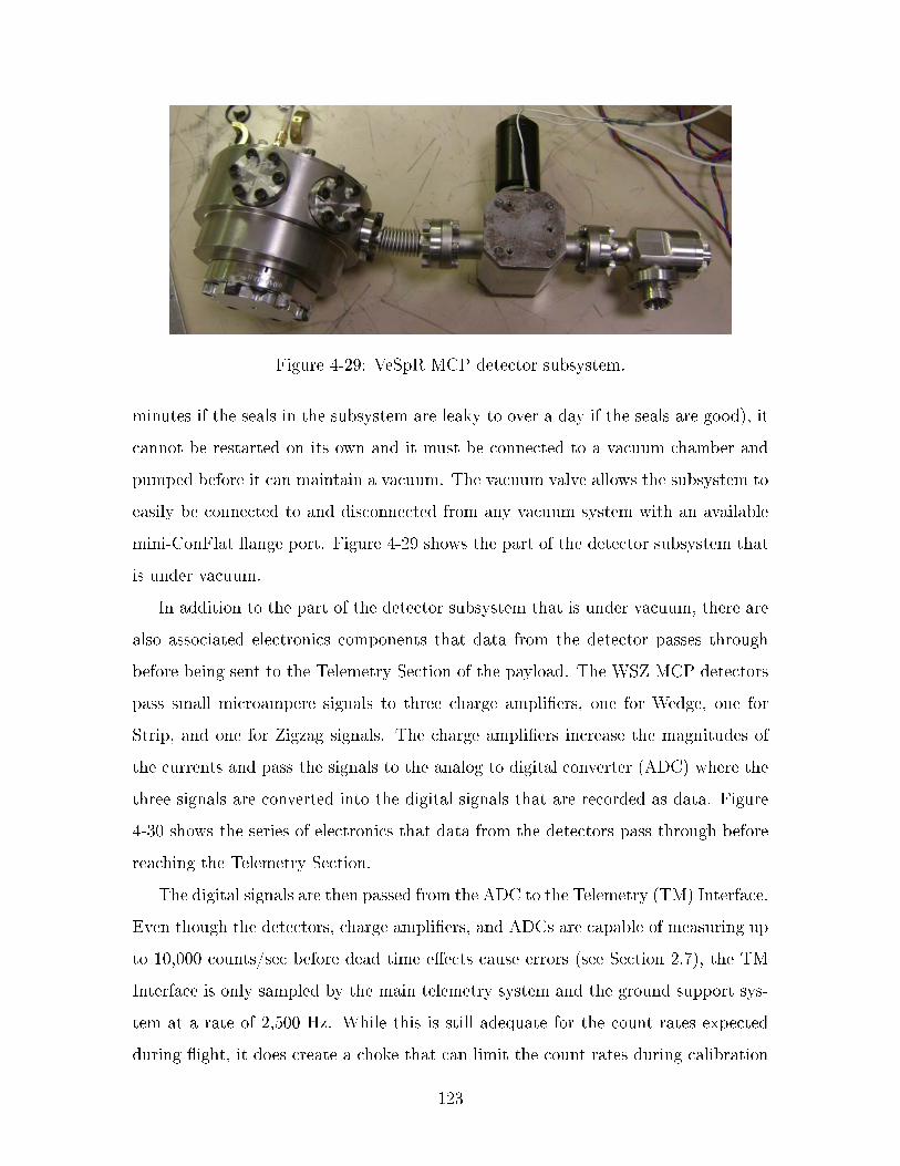
Figure 4-29: VeSpR MCP detector subsystem.
minutes if the seals in the subsystem are leaky to over a day if the seals are good), it
cannot be restarted on its own and it must be connected to a vacuum chamber and
pumped before it can maintain a vacuum. The vacuum valve allows the subsystem to
easily be connected to and disconnected from any vacuum system with an available
mini-ConFlat ange port. Figure 4-29 shows the part of the detector subsystem that
is under vacuum.
In addition to the part of the detector subsystem that is under vacuum, there are
also associated electronics components that data from the detector passes through
before being sent to the Telemetry Section of the payload. The WSZ MCP detectors
pass small microampere signals to three charge ampliers, one for Wedge, one for
Strip, and one for Zigzag signals. The charge ampliers increase the magnitudes of
the currents and pass the signals to the analog to digital converter (ADC) where the
three signals are converted into the digital signals that are recorded as data. Figure
4-30 shows the series of electronics that data from the detectors pass through before
reaching the Telemetry Section.
The digital signals are then passed from the ADC to the Telemetry (TM) Interface.
Even though the detectors, charge ampliers, and ADCs are capable of measuring up
to 10,000 counts/sec before dead time eects cause errors (see Section 2.7), the TM
Interface is only sampled by the main telemetry system and the ground support sys-
tem at a rate of 2,500 Hz. While this is still adequate for the count rates expected
during ight, it does create a choke that can limit the count rates during calibration
123

Figure 4-30: Detector data processing electronics leading to the Telemetry Section ofthe payload.
testing since the maximum measureable count rate using the ground support comput-
ers is 2,500 counts/sec. For all calibration tests, the calibrating lights were dimmed
so that the count rate was below this threshold.
4.2.3 Power Subsystem
The power distribution subsystem of VeSpR is complex because there are so many
dierent power requirements in so many dierent systems. In addition, because the
payload has been modied so much over the last four decades, some power systems
and wiring harnesses are still in the payload. Removing some of these harnesses
would require more work than the decrease in payload mass would be worth, and
some obsolete components in the power subsystem are associated with components
that are still required in the operation of the payload.
There is not one single gure that fully encapsulates every aspect of the power
system, but there are a series of gures that can adequately describe the system as
a whole. There are two main hubs where most of the payload's required power is
received and distributed throughout the payload, the Old Low Voltage Power Supply
(OLVPS) and the New Low Voltage Power Supply (NLVPS). There are three plugs
that supply power to the payload; two of them are umbilical cables that connect
through the Spectrometer and Spectrometer Extension skin sections of the payload,
124

Figure 4-31: Old Low Voltage Power Supply (OLVPS) and a block diagram of itscomponents.
and the other supplies battery power through the Interface Plate.
The rst umbilical cable connects through the Spectrometer Extension skin section
and directly supplies 28V power to the OLVPS from an outside power supply. This
umbilical can be used on the launch pad or during integration testing to power the
payload without using power supplied by the payload batteries. The OLVPS consists
of a control module, a preregulator, a converter, and several output modules, all
connecting through a single Bendix connector. Figure 4-31 shows the OLVPS and
the Bendix connector routing all the inputs and outputs on the OLVPS and a block
diagram of the modules it contains.
An example of an obsolete system still operating in the payload is the ±15 V power
supply. There are no longer any components that operate at ±15 V, but removing the
±15 V power supply would require the three most complex connectors in the entire
payload to be remade.
Figure 4-32 shows a block diagram of the distribution of 28 V power in the payload
as it is being supplied from the rst umbilical cable (top left). This diagram is taken
directly from the updated wiring notebook and is meant to show how power is direct
within the payload; it does not show accurate locations of the various modules and
connectors. For instance, the connection P20/J20 is shown twice, and the three sides
of the control module are actually coming from a single connector. Green lines in
125

Figure 4-32: 28V power supply chain through the OLVPS. The green lines representunregulated input power wires, the red lines represent regulated internal power wires,and the black lines are ground wires.
the diagram represent wires carrying unregulated 28 V external power. Red lines
represent regulated 28 V internal power. Black lines represent ground wires.
Notice the current monitor and battery connector on the right side of the diagram.
If power was being supplied from the battery, it would similarly go through the control
module and into the preregulator before being distributed back into other payload
systems.
The high voltage expansion plate controls the power input to the MCP detector
high voltage power supplies. Switching power on to these supplies can be done with
126

Figure 4-33: 20 V and 5 V power chains through the OLVPS.
the ground support system (see Section 4.2.6) or by the Telemetry Section of the
non-science part of the payload. The transistor switch board is controlled similarly
to activate the ight computer, labeled PC in Figure 4-32. The ight computer
contains its own DC/DC 28V/5V power converter and electromagnetic interference
(EMI) lter. Also notice the NLVPS in Figure 4-32, labeled DC/DC +12/+5V Power
Supply. This will be described later in this section, but note its location relative to
the OLVPS in the power supply chain.
Figure 4-33 shows two more power chains provided by the OLVPS, the 5 V and
±20 V chains. Other power chains are not shown but behave in a similar manner, with
external power passing through the control module, preregulator, and the converter
before being passed to various other power regulators supplying dierent voltages.
The NLVPS receives 28 V regulated power from the OLVPS. The NLVPS has two
±12 V power supplies, one 5 V power supply, and one EMI lter that lters the input
to the ±12 V supplies (more on this later). Figure 4-34 shows the NLVPS as it is
mounted in the payload, and Figure 4-35 shows a solid model of the NLVPS as it was
127

Figure 4-34: NLVPS mounted in the payload.
before modications were made (see Section 5.2.4).
The NLVPS supplies power to MCP detector's electronics and allow for data to
be transmitted from the detectors to the Telemetry Section of the payload. The ±12
V power needs to be ltered because it supplies power to the charge ampliers, and
even small variations in the current supplied to the ampliers can have a tremendous
impact on the quality of the data as it moves from the charge ampliers to the ADCs.
The 5 V power only supplies digital electronics, which are robust enough to not require
EMI ltering.
Data from the spectrograph is also fed through the ight computer, through an RS-
422 converter, and out of the second umbilical cable so that it can be read separately
from the rest of the ground support system or any WFF electronics; however, since
the ight computer is broken, this data chain is obsolete. Figure 4-36 shows a block
diagram of the NLVPS system and the components it distributes power to.
The detector high voltage supplies, shown as HV1 and HV3 receive power
from the high voltage expansion plate, which is not shown in Figure 4-36, but every
128

Figure 4-35: Solid model of the NLVPS.
Figure 4-36: NLVPS block diagram and components that are supplied by the NLVPS
129

other component shown receives power from the NLVPS.
The remaining power input to the payload comes through the second umbilical
cable located in the Spectrometer section. The second umbilical cable supplies 28
V power to the VIP high voltage power supplies. This power connection is never
interrupted while the payload is assembled because if power is cut for long periods of
time, air will slowly leak into the detector subsystem and the VIPs will not be able
to maintain a vacuum when they are powered on again. While the rocket is on the
launch pad, this umbilical supplies power to the VIPs to keep the detector housings
at vacuum until launch.
This presents unique challenges when shipping the payload; historically, the pay-
load has been transported in a moving truck and a power supply is brought along
and connected to the cigarette lighter. A cable is connected through the cabin to the
back of the truck into the payload storage container where the VIP control box is
located. The VIP control box has wires that run through the second umbilical cable
and supply power to the VIP high voltage power supplies.
Power to the VIPs can be disconnected for short periods of time without endan-
gering the detectors or making it impossible to restart the VIPs; in fact, the reason
power is supplied by an umbilical is because the VIPs are powered up until launch.
For the duration of the mission, the VIPs are turned o. The VIPs must be turned o
during the mission and during testing because ions from the VIP go into the detector
and add a signicant amount of noise to the data.
4.2.4 Analog Monitor Subsystem
There are a number of analog monitors throughout the payload that provide infor-
mation on how the payload is operating through the telemetry stream that can be
monitored in real time during ight or during testing. There are voltage, current,
temperature, and pressure monitors throughout the payload.
The most common analog monitor is the voltage monitor. There are voltage
monitors on every high voltage power supply and every low voltage power supply. All
of the supplies have a built-in monitor that outputs a voltage that is indicative of the
130

load on the supply. In the high voltage power supplies, the monitors take the output
voltage and divide it by 2000; for instance, a high voltage power supply operating
at 4500 V would have an output monitor voltage of 2.25 V. The low voltage power
supplies have either no voltage division for the 5 V power supplies or are divided by
3 on the 12 V power supplies, so the proper monitor voltage for a 12 V supply is 4 V.
There is a current monitor box that monitors the total current running through
the 28 V supply system that operates whether power is supplied externally through
the rst umbilical or internally through the battery supply. This monitor is the best
indicator of the overall health of the payload when all systems are powered. If the
current deviates slightly from the measured test value, there is most likely at least
one voltage monitor that is also deviating from the measured test value.
Thermisters are used in various sections of the payload to monitor internal temper-
ature during the ight. These monitors were added for an earlier ight because there
was concern that the temperature variations during ight would aect the optical
properties through thermal expansion, but ight data showed that the temperature
changes inside the payload were minimal and did not contribute to any problems.
The thermisters are still on board the payload as an extra experimental measure-
ment. However, there are no thermisters inside any of the electronic components, so
careful monitoring of the thermisters would not have prevented any electronics from
failing during testing for the previous ight (see Section 4.4).
Finally, there is a barometer switch inside the payload. Most suborbital payloads
are vacuum sealed, but VeSpR only requires that the MCP detector subsystems op-
erate in vacuum for the entire ight. Vents in the payload skin sections allow air to
escape, so a pressure sensor inside the payload can feed data through the telemetry
to decide when to open the shutter door and power on the MCP detectors. This
pressure sensor/altitude switch is mounted to the Interface Plate.
4.2.5 Structure Subsystem
The payload is split into six total sections and two distinct halves; one half contains
the telescope and the other half contains the instruments and electronics. These two
131

halves are connected by a large center plate. All six sections of the payload have
their own external skin sections that provide protection from external elements and
structural support during launch. These skin sections are standard for most WFF
suborbital ights and can be replaced easily in the event that one of them takes too
much damage to be safe for ight. The skin sections connect to each other and to
the large center plate at the center of the science payload.
Figure 4-37 shows the three instrument (non-telescope) sections of the payload as
they are without their skin section covers. The three sections from top to bottom
are the Spectrometer Extension section, the Spectrometer section, and the MCP
Detection section (see Figure 4-2 for where these sections are located within the full
payload). The three sections that comprise the telescope half of the science payload
would be beneath the sections in the gure, and the telescope would be pointing
downward.
The three instrument sections are supported and connected by three longirons
that span the length of this half of the science payload and connect to the center
plate. Various other plates and electronics housings are also attached to the longirons.
Teon shims are mounted on the outward-facing sides of the longirons. When the
skin sections cover the payload, the Teon shims hold the skin sections in place and
prevent vibration damage.
At the top of Figure 4-37 is the Interface Plate. If the full payload were assembled,
the Telemetry Section would be above the Interface Plate. Figure 4-38 shows all of
the connections on the Interface Place and their labels as they were at the beginning
of the project.
Beneath the interface plate, two plates hang down and are connected by standos.
The rst is the Semicircular Plate, and the second is the Boomerang Plate. The
OLVPS, the current monitor, and connector J20, the largest connector in the rocket
and the one that has the most power connections, are mounted on the top of the
Semicircular Plate. Several other connectors are mounted to the bottom of the plate.
The Boomerang Plate was built to be an expansion to the Semicircular Plate and
has other connectors mounted to the bottom of it as well. Both sets of standos that
132

Figure 4-37: Side view of the Spectrometer Extension (top), Spectrometer, and MCPDetection Sections of the payload without their skin sections (see Figure 4-2 forcontext).
133

Figure 4-38: Original conguration of the connectors on the Interface Plate.
hold the plates are used to secure wire harnesses. Figure 4-39 shows the Semicircular
Plate and the Boomerang Plate.
Beneath the two hanging plates is a structural plate that separates the Spec-
trometer Extension section from the Spectrometer section. On this plate, the ight
computer and NLPVS are mounted. In addition, a hole is cut out in this plate where
the spectrograph box extends through. Teon supports are mounted to the edges that
hold the long spectrograph box in place and prevent it from being bent out of align-
Figure 4-39: Semicircular Plate (left) and Boomerang Plate (right)
134

ment during launch. This plate is bolted to the three longirons, and it is at these
locations where the Teon shims are mounted that prevent the skin sections from
vibrating against the rest of the structure. The RS-422 converter and VIP control
module are mounted to the bottom of this plate.
At the bottom of the Spectrometer section, there are two plates. The top plate
holds the VIP high voltage power supplies and one set of charge ampliers. The bot-
tom plate marks the bottom of the Spectrometer section, where the other set of charge
ampliers, the bottom of the spectrograph box, and the high voltage expansion plate
are mounted. The spectrograph box also serves as structural support for mounting
electronics. Both sets of ADCs and TM Interfaces are mounted to the broad sides of
the spectrograph box.
Beneath the Spectrometer section is the MCP Detection section, which contains
the Imager box, both detector subsystems, the Xybion camera, the SPACOM star
tracker, the accelerometers, and the secondary mirror control box. Some of these
modules are mounted to the longirons, but the Imager box is mounted to the center
plate that divides the experiment section from the telescope section and the plate
that the Spectrograph box is mounted to because it is so heavy.
On the other side of the center plate is the telescope. Aside from the tripod that
supports the secondary mirror of the telescope, the three telescope sections are nearly
empty and mostly serve as a bae to prevent light from entering the system. The
only other equipment in these sections are the telescope's heat shield, the mount
for the ST-5000 star tracker in the Telescope Extension section, and cables that run
through the center plate to power the secondary mirror servos and the ST-5000.
The science payload uses only passive thermal control elements to keep the tem-
perature in the payload manageable. The heat shield surrounding the telescope pre-
vents thermal expansion from changing the optical properties of the telescope, but
otherwise no elements are in the payload solely to manage heat.
In a vacuum, there is no air to convectively transport heat energy, so conduction
and radiation are the only heat transfer mechanisms. Radiative heat transfer is
inecient, especially below the maximum operating temperature of most electronic
135

components, so conductive heat transfer is the best way to prevent overheating within
any electronics in vacuum. Potting and thermal grounding are used to lessen the risk
of heat buildup in VeSpR's electronics.
Electronics potting is a practice where an electronics assembly is lled with a
solid compound, such as epoxy, silicone, or polyurethane. This greatly increases the
assembly's resistance to shock and vibration damage, but if a compound with high
thermal conductivity is used it has to added advantage of dissipating heat from the
electronics. While conformal coating is often used to protect electronics in standard
environments, it does not provide enough protection for electronics in spaceight
applications.
Every electronics board on VeSpR is potted. In addition, the structures the elec-
tronics are mounted in are designed with more mass than what would be optimal to
survive the loads experienced in ight. Because they are more massive, they have a
higher total heat capacity and can act as heat sinks for the electronics. While the
heat transfer properties of the payload have never been formally modeled, no elec-
tronic equipment has failed in a previous ight due to heat damage. In practice, the
electronics are never left powered on for much longer than the length of the ight
when they are being tested in vacuum. Components have been damaged in testing
in the past (see Section 4.4).
4.2.6 Ground Support Equipment
The existing VeSpR ground support equipment (GSE) is overly complex for what is
needed for testing, but it was built to be a realistic simulation of the payload as it
is congured in ight. Figure 4-40 shows the two GSE computers used to interpret
data from the payload and the GSE control suitcase used to control and power the
payload.
Data from the imager, spectrograph, and analog monitors all ow through con-
nectors on the Interface Plate at the top of the payload and into the spaghetti box,
a module that contains a WFF-93 Pulse Code Modulator (PCM) stack exactly like
the one used in ight. The PCM stack then transmits the data through a bit sync
136

Figure 4-40: GSE computers (left) and control suitcase (right).
encoder that simulates the transmission of data through an antenna and feed it into
the rst GSE computer.
The rst ground support computer runs a copy of TD+, the telemetry program
that WFF used in previous JASpR ights. It displays all analog monitors and counters
from the detectors. Although it does not directly display data from the detectors, the
detector operation can be monitored by examining the counts coming through the
TD+ interface.
Data from the detectors is sent from the rst GSE computer through a buer box
into the second GSE computer, which is where data is displayed in real time during
calibration testing. Figure 4-41 shows an example of data from a calibration test
being shown on the second GSE computer.
Real time information that is displayed includes the total photon counts, the
current count rate in counts per second, the total number of rejected counts, and the
total number of bad counts. In this particular test, there was excessive background
noise because the VIP was not turned o before the detector high voltage power
supply was turned on. The thick line running diagonally on the screen in Figure
4-41 is a line prole generated from a Mercury lamp and is similar to a hydrogen
Lyman-alpha line prole that is seen in testing and in ight.
Most of the functions on the GSE suitcase are obsolete, but the two most impor-
tant functions of the suitcase are still operational. Two protected switches control
137

Figure 4-41: Display of the second ground support computer showing data in realtime from a calibration test.
power to the MCP detector high voltage power supplies while the payload is on the
ground for testing. There are various ports that voltmeter probes can be plugged
into to measure analog voltages without needing the GSE computers and the TD+
output. The suitcase also controls the input power through the rst umbilical cable,
but that can be supplied without the GSE suitcase if needed.
4.3 Laboratory Facilities and Challenges
There are a number of facilities at Boston University that were needed to prepare
VeSpR for ight. The three primary laboratory facilities that are being used through-
out Project VeSpR are the Vacuum Calibration and Testing Facility (VACTEF), the
Vacuum Ultraviolet Calibration Laboratory (VUCL), and the Ultraviolet Electronics
Laboratory (UVEL).
138

4.3.1 Challenges with Vacuum Chambers and Ultraviolet Test-
ing
Ultraviolet light is absorbed by Earth's atmosphere, which is why the D/H ratio of
Venus cannot be constrained with a Lyman-alpha measurement from a ground tele-
scope. The absorption of ultraviolet light by the atmosphere also makes it dicult to
test the performance of VeSpR on the ground. Ultraviolet testing must be performed
in vacuum chambers where the pressure is low enough for ultraviolet light to travel
without interference from air molecules.
Vacuum chambers are complex systems with performances that vary greatly from
one system to the next. Some do-it-yourself systems can be very cheap but only
achieve low pressures comparable to what airliners experience in the stratosphere.
Large systems that can achieve pressures comparable to deep space cost a signicant
amount of money. In general, the larger the system and the lower the pressure
required, the more expensive the systems are.
4.3.1.1 Types of Vacuum Pumps
There are a number of dierent types of vacuum pumps. The cheapest and least
eective are standard scroll pumps. Scroll pumps act like fans with valves that blow
air out of the system and are eective at reaching pressures in the 1-10 Torr range (at-
mospheric pressure is 760 Torr). However, scroll pumps are used as primary vacuum
pumps in most vacuum systems because most of the more sophisticated pumps that
can achieve lower pressures actually require low pressures before they can even be
turned on. Scroll pumps are used as the primary pumps in all three vacuum chamber
systems at Boston University. Figure 4-42 shows a scroll pump.
Turbomolecular pumps (or turbopumps), like scroll pumps, use fan-like blades to
move air out of the system. Unlike scroll pumps, turbopumps operate at supersonic
speeds and use shockwaves to impart momentum to gas particles to move them out
of the system. Turbopumps can be expensive and require a sophisticated power
controller. Small turbopumps have a tendency to fail easily because they must spin
139

Figure 4-42: Scroll pump used in the VACTEF as the primary vacuum pump.
Figure 4-43: Turbomolecular pump used in the UVEL vacuum chamber (left) and itspower controller under normal operation (right).
at a higher rate to achieve shockwaves at the tips because of the smaller radius
compared to turbopumps with a larger diameter. Depending on the size, turbopumps
can achieve pressures as low as 10-11 Torr. Turbopumps are used in the VUCL in
the light source of the monochromator, and in the UVEL as the secondary vacuum
pump. Figure 4-43 shows a turbomolecular pump and its power controller.
Another type of vacuum pump that achieves low pressures is a cryogenic pump.
Rather than moving gas molecules out of a system entirely, like the turbo and scroll
pumps, cryogenic pumps instead act as gas traps that capture moving molecules and
freeze them in place. Cryogenic pumps are helium-cooled and reach temperatures
very low temperatures. How eective cryogenic pumps are depends on the freezing
temperature of the gasses in the chamber, but when vacuuming air with cold traps at
140

Figure 4-44: Cryogenic vacuum pumps used as the secondary vacuum pumps inthe VACTEF (left) and the power control and helium cooling unit that control thecryogenic pumps (right).
10 Kelvin, these can be very eective pumps, reaching pressures as low as 10-10 Torr.
While they are expensive and do not achieve quite as low a pressure as turbopumps,
they are low-maintenance, have fewer moving parts, and are overall more robust, since
failures do not cause catastrophic internal damage to the pumps. Cryogenic pumps
are used in both the VACTEF and VUCL as the secondary vacuum pumps. Figure
4-44 shows three cryogenic pumps and their helium cooling unit and power supply.
A fourth common type of vacuum pump is the diusion pump. Diusion pumps
use a high-speed jet of gas to move gas molecules at the top of the pump down to the
bottom and out the exit. Usually, these pumps use some kind of oil as the working
uid. Diusion pumps are extremely reliable and have no moving parts, and they
can achieve pressures as low as 10-10 Torr. Figure 4-45 shows a schematic diagram of
a diusion pump. However, despite these advantages, diusion pumps are forbidden
from being used in any vacuum chamber that any component of the VeSpR will be
tested in because oil contamination degrades the ultraviolet reective and throughput
eciencies of optical components.
4.3.1.2 Ultraviolet Testing in Vacuum
The biggest challenge with most vacuum systems is making sure they are airtight.
Any vacuum system is only as good as its weakest seal, and some systems may have
hundreds of seals. If a feedthrough plate is misaligned or the O-ring is not seated
141

Figure 4-45: Schematic diagram of how a diusion pump operates.
properly there will be a leak. It is particularly hard to seat O-rings properly when
they are vertical.
Finding a leak in a vacuum system can take days, and it usually involves one
person systematically squirting isopropanol all around every vacuum seal while an-
other person watches the vacuum gauge to see if there is a change in pressure. If
isopropanol is sprayed on a leaking seal, the liquid isopropanol will slowly enter the
system instead of the gaseous air, which quickly brings down the system pressure as
isopropanol continues to ll the leak. After some time, the isopropanol will evaporate
and the pressure will rise again.
The best leak-checking procedure is to use a mass spectrometer and a helium
spray. Mass spectrometers measure the mass-to-charge ratio of particles and can
identify the molecular weight of molecules. Helium is an inert gas and has a small
radius compared to most gas molecules, which means it can easily enter a vacuum
system through a leak. If a mass spectrometer is in use in a vacuum system, leaks
can be found by spraying the seals with helium and watching for a spike in particles
with four atomic mass units the mass of a helium atom. There should be very little
helium in the system before helium gets sprayed on a leak, so if there is a sudden
spike, a leak has been found. Mass spectrometers are also useful in identifying the
142

constituents of the gas and determining the level of contamination in the system.
In most applications, the cleanliness of a vacuum system is usually not an issue.
Most vacuum seals that use Viton or rubber O-rings are coated with vacuum grease to
prevent leaks. Diusion pumps tend to put some small amount of the working uid,
usually oil, into the system. A ngerprint inside a vacuum chamber will not drastically
aect how quickly the chamber reaches its operating pressure if the minimum pressure
of the system is two or three orders of magnitude lower so its impact on system
performance is negligible.
Ultraviolet vacuum testing is very dierent. The reason why ultraviolet astronomy
cannot be done on the ground is because Earth's atmosphere absorbs ultraviolet light.
However, ultraviolet light is absorbed even more eectively by hydrocarbons. Not
only do hydrocarbons absorb ultraviolet light eectively, the energy of the ultraviolet
light can cause photochemical reactions that produce bigger hydrocarbons, a process
called polymerization. These bigger hydrocarbons block ultraviolet light even more
eectively.
Because of this, hydrocarbon contamination is a huge concern when dealing with
ultraviolet optics. Even a monolayer of hydrocarbons on an optical surface can de-
crease its eciency (whether it is reective or transmissive eciency) by a huge
factor, enough to make that optic essentially useless. Cleaning ultraviolet optics is
very dicult and often results in the optic being replaced in the end.
Despite the fact that its instruments were working properly, the ight prole was
accurate, and all targets were observed for longer than the minimum required time, the
JASpR V ight was deemed only a partial success rather than a full success because
the overall optical eciency of JASpR was much lower during ight than it was during
calibration testing. The reason for this sudden and unexpected degradation of the
optics was due to some nal testing that was done in a vacuum chamber that used
diusion pumps as the secondary vacuum pumps.
Under normal operating conditions, diusion pumps can be used to pump down a
vacuum chamber without contaminating the system or any ultraviolet optics inside.
However, if the vacuum valves and pumps are not operated correctly, oil can back-
143

stream into the chamber. During JASpR testing, maintenance on one of the diusion
pumps was performed while the system was at vacuum. Before the pump was turned
back on, the vacuum valve that connects the pump to the chamber was opened. At
this point, the pressure in the vacuum chamber was lower than the pressure at the
diusion pump inlet. This error caused a small amount of oil to be displaced into the
vacuum chamber, which, in a gaseous state, expanded into the chamber and diused
into the payload and optics, coating the surfaces with hydrocarbons. Since then,
great care has been taken to ensure that contamination of this sort does not happen
again.
This is why all of the vacuum chambers that VeSpR uses for testing have been
specically designed to not use oil. Most of the vacuum chamber seals use copper O-
rings instead of Viton or rubber. Viton and rubber O-rings work well when they are
coated with vacuum grease, but even low-outgassing vacuum grease is a contaminant
that is undesirable in the system. Copper O-ring performance exceeds that of Viton
and rubber O-rings if vacuum grease is not used. The only vacuum pumps that are
used are the types that do not use any hydrocarbon oil whatsoever (scroll, turbo, and
cryogenic pumps).
The inside of the vacuum chamber used in ultraviolet testing is kept very clean.
Great care is taken to ensure that no ngerprints are made inside the chamber because
ngerprints are composed of hydrocarbons. If any ngerprints are put on the inside
walls of the vacuum chamber, they are cleaned with isopropanol before the vacuum
chamber is brought to low pressures. Gloves are worn at all times when loading
equipment into the vacuum chamber and handling system components like O-rings
and vacuum anges.
Any part that is manufactured in a machine shop tends to be coated with machine
oil. Before any new component fresh from machining is put in a vacuum chamber or
even attached to other components that will go in a vacuum chamber, it is cleaned.
First, it is scrubbed with soap and water to get most of the contaminants o the
surface. Next, it is bathed and scrubbed in isopropanol, then acetone. Finally, the
component is put in an ultrasonic bath before it is cleared to enter a vacuum chamber.
144

Figure 4-46: The vacuum chamber in the Vacuum Testing Facility (VACTEF)
4.3.2 The Vacuum Calibration and Testing Facility (VACTEF)
The VACTEF was specically built to test the VeSpR payload, and most of the
VeSpR documentation, testing equipment, tooling, and other essentials are stored
here. The primary purpose of the vacuum chamber in the VACTEF is to test the
VeSpR payload in a space-like environment. The vacuum chamber is 18 feet long and
3 feet in diameter, large enough to t the entire payload in. It has one scroll pump
for low vacuum and three cryogenic pumps for high vacuum. A light source chamber
installed at one end of the main chamber can house a variety of optics and light
sources for testing ultraviolet optics and detectors. Figure 4-46 shows the vacuum
chamber in the VACTEF and Figure 4-47 shows a block diagram view from the side.
145

Figure 4-47: Block diagram of the vacuum chamber. C: Cryogenic Pumps; P: Ports;L: Ultraviolet Lamps; T: Thermocouple vacuum gauge; I: Ion vacuum gage; S: Sparesmall port; M: Manual leak valve. Sliding Rails allow the payload to be set on amount with Teon-lined supports so that it can be easily slid further into the vacuumchamber.
4.3.2.1 Systems Overview
The vacuum chamber has pneumatic, electric, and manually actuated valves. The
pneumatic valves are all either normally-open or normally-closed, depending on what
direction the valve needs to go in the event of a power outage such that the valves
would open or close on their own to prevent damage to the parts they connect to the
chamber. An air compressor and hose system connects all the valves. The pneumatic
and the electric valves are all controlled from a panel near the center door. The
manually actuated valves are used only for venting the system and bringing it up to
atmospheric pressure.
The cryogenic pumps require cold water to regulate the temperature of the pump's
power supply. The water-cooling system routes from the power supply to a ow
switch, up through the ceiling, and to an outside water chiller. This chiller occasion-
ally breaks down and the cryogenic pump overheats, but it will automatically shut
itself o if the internal temperature goes above 110 degree Fahrenheit.
The volume of the system that experiences vacuum is split into two sections,
the main chamber and the forelines. The forelines connect the scroll pump to the
cryogenic pumps and the main chamber. At the start of operations, the exhaust
valve is opened, the scroll pump is turned on, and the foreline valve opens. When
the pressure in the forelines goes below 1 Torr, the cryogenic forevalves are opened
146

and the cryogenic pumps are brought down to vacuum. When the pressure goes
does below 1 Torr again, the cryogenic forevalves are closed, the cryogenic pumps are
powered up, and the main chamber is opened to the scroll pump.
The cryogenic pumps require approximately an hour and a half to cool down to 5
Kelvin, and the scroll pump takes approximately half an hour to pump the chamber
down to 1 Torr. Once both of these states have been achieved, the foreline valve
is closed and the primary cryogenic valves are opened. With the cryogenic pumps
exposed to the main chamber, the pressure quickly drops down to operating levels. If
the chamber is empty and freshly cleaned, and if none of the copper O-rings are being
reused (they are supposed to be replaced every time a seal is opened), the vacuum
system can achieve pressures as low as 5 x 10⁻⁹ Torr. The average operating pressure
in the vacuum chamber during testing when the payload and other equipment are
inside is 5x10⁻⁷ Torr, which is lower than the pressure of the atmosphere at 110 km
altitude (about 1x10⁻⁴ Torr)
There are three vacuum gauges that measure the pressure in the system. Two
are thermocouple (TC) gauges. One is mounted in the forelines on the back of the
chamber, and the other is mounted on the top of the chamber (T in Figure 4-47).
These gauges accurately measure the pressure in the system down to approximately
10-3 Torr. Beneath this pressure, the TC gauges are no longer accurate. The third
pressure gauge is the ion gauge (I in Figure 4-47), which accurately measures pres-
sure from 10-4 to 10-11 Torr. This gauge cannot be turned on if the pressure is above
10-4 because the lament will burn out and need to be replaced.
Even though there is an order of magnitude pressure dierence between the ranges
of these two types of gauges, it does not matter, because when the cryogenic pumps
are opened up the chamber pressure drops from ~1 to ~10-5 Torr in a matter of
seconds and continues dropping after that.
4.3.2.2 Final Systems Design and Building
At the beginning of work on Project VeSpR, the vacuum chamber was inoperable.
While all of the hardware components were installed (pumps, hoses, forelines, etc.),
147

Figure 4-48: Wiring Schematic of the quartz lamps.
major electrical work needed to be done to bring the system online. Most of the
electrical parts had been purchased, but the exact wiring had not been designed. The
entire control board needed its wiring to be designed and built as well.
The vacuum chamber uses 240V A/C to power the cryogenic pumps, 120V to
power the scroll pump, air compressor, gate and switch valves, ultraviolet lamps,
and other heavy duty equipment, and 12V to power the relays, LEDs, ow switches,
and other minor components. Figures 4-48, 4-49, 4-50, 4-51, and 4-52 show some of
the schematic designs of the wiring of various systems for the vacuum chamber. All
designs were made in XCircuit.
Once the schematic designs were nished and inspected, the wiring harnesses were
constructed. Figure 4-53 shows the stark contrast between what is seen at the front of
the control panel and relay switchboard and the complex wiring that is immediately
behind both. Figure 4-54 shows the 12 V buses that send power from the 12V power
supply to every LED on the panel and every other component that operates at 12V.
Before this wiring work was completed, the valves were actuated manually using a
C-clamp, and there was no monitoring system to see whether the valves were operating
properly. Once work was completed, the entire system could be operated from the
control panel, and any failure point in any valve could be seen because of the LED
148

Figure 4-49: Wiring schematic of the 240V relays that supply power to the cryogenicpumps.
Figure 4-50: Wiring schematic for the LEDs on the control panel.
149

Figure 4-51: Wiring schematic of the valves that control the cryogenic pumps. Fore-line valves open the pumps to the scroll pump and forelines while the chamber valvesopen the cryogenic pumps to the main chamber.
Figure 4-52: Wiring schematics of the pneumatic pressure and ow switch sensorLEDs.
150

Figure 4-53: Front view of the control panel and relay switchboard (left) and the viewfrom behind the panels (right).
Figure 4-54: 12V buses and 12V power supply. This is a view that is slightly tothe left of the view shown in Figure 4-53(right). The black box in the bottom rightcorner of Figure 4-54 and the top left corner of Figure 4-53(right) is the vacuum gaugecontrol box.
151

status lights. The simplied operating instructions were written out and attached
beside the control panel. The full text is available in the attached Appendix DVD.
4.3.2.3 System Maintenance
Thoroughly cleaning the inside of the chamber is more dicult that one might imag-
ine. A person must don a full clean suit, usually disposable, complete with booties,
gloves, hairnet, and face mask, and crawl into the chamber. Smaller people are better
for cleaning, but it is still dicult to maneuver inside the chamber. Both doors are
opened to allow for maximum air circulation inside the chamber while the cleaner is
inside. The cleaner must spray isopropanol onto all surfaces and wipe them down.
The dangerous part about this is working in an enclosed environment while spray-
ing toxic chemicals. The cleaner must have someone on the outside supervising be-
cause isopropanol fumes will intoxicate and possibly suocate the cleaner if the cleaner
uses too much isopropanol or stays in the chamber for too long. Even with proper
care, the person cleaning the chamber will most likely feel hung over once the job is
done without experiencing a state of drunkenness rst like one would expect before
a hangover.
After the inside is cleaned, the chamber is pumped down to high vacuum and
the quartz lamps are turned on. The quartz lamps emit high-energy ultraviolet light
that breaks down any contaminant molecules left on the inside of the chamber. This
is much faster than simply pumping on the contaminants and waiting for them to
evaporate on their own. Removing contaminants also makes the pressure go down
faster since nothing is left to evaporate and articially keep the pressure higher. While
the major concern for contaminants is hydrocarbons, water contamination can make
pumpdown times increase dramatically while the water gradually evaporates into a
gas from a much denser liquid state.
The cryogenic pumps use liquid helium to cool the system, but helium is notorious
for its high leak rate as a result of its small atomic radius. The helium tank on the
cryogenic pump power supply needs to be relled occasionally. Relling is a non-
trivial process that requires care not to contaminate the entire helium supply with
152

Figure 4-55: The vacuum chamber and the monochromator viewed from outside ofthe clean room.
other air particles that would freeze at much higher temperatures in the cryogenic
system than the helium would. On two occasions a rell was needed, and in both
cases no harm was done to the system.
4.3.3 Vacuum Ultraviolet Calibration Laboratory (VUCL)
The VUCL houses a vacuum chamber that is 5.5 feet in diameter and 8 feet long.
Inside the chamber, there is a ne-motion optical table with three axes of motion
controlled from an external computer. On one side of the main chamber is a light
source chamber with a monochromator. The other side has a large door that is the
main entrance to the chamber that is housed in a clean room. Figure 4-55 shows the
vacuum chamber and monochromator from outside the clean room, and Figure 4-56
shows the vacuum chamber from inside the clean room.
153

Figure 4-56: Views of the vacuum chamber from inside the clean room (left) and theoptics table inside the vacuum chamber (right).
Figure 4-57: Areas of the vacuum chamber that leak. (left) A feedthrough platewith poorly-installed D-subminiature connectors. (right) A gate valve beneath thecryogenic pump.
The vacuum chamber uses a scroll pump as its primary pump and one large cryo-
genic pump as its secondary pump. While this vacuum chamber was certainly the
most well-equipped vacuum chamber for calibrating each optic individually, opera-
tions were very dicult due to a variety of problems.
This vacuum chamber is not very well sealed. There are at least two major leaks,
the rst of which is from a feedthrough plate that uses D-subminiature connectors
that were badly installed but are vital to the work the VeSpR team was doing, so
it could not be replaced with a more robust plate. The second is the gate valve
that separated the cryogenic pump from the main chamber. Due to these leaks, the
chamber never able to achieve a pressure below 10-6 Torr. Figure 4-57 shows these
two leak locations.
154

In the VACTEF, the cryogenic pumps can be opened and closed and the vacuum
chamber can be brought up to air multiple times before the cold traps became too
full to eectively maintain high vacuum, after which they need to be recharged and
vented. The recharge cycle time on the VACTEF cryogenic pumps is on the order of
three hours.
In the VUCL, the vacuum leaks take their toll on system performance. Because
the lowest achievable pressure is still over an order of magnitude higher than the
normal operating pressure of the VACTEF vacuum chamber, the cold traps in the
cryogenic pump ll up very quickly. Because the leak in the gate valve is worse, the
cryogenic pumps can only be used for one pumpdown before needing to be recharged.
In addition, the cryogenic pump on this vacuum chamber has a recharge cycle time
of 24 hours, so not only is the pressure barely adequate to do ultraviolet calibration
testing to begin with, it also takes over a full day between measurements.
For each measurement, a person would have to suit up, enter the clean room,
adjust the optics, reseal the chamber, and come out. Afterward, the chamber would
be pumped down and the measurement would be taken, then the cryogenic pump
would be full and the pressure would start to rise. The chamber would be brought
back up to air and the cryogenic pump would be recycled, and after 24 hours the
cryogenic pump would be ready to go again, all so that a person could crawl back in
the chamber and make a small, sometimes sub-millimeter adjustment to an optic on
the table.
Another major problem with using this vacuum chamber was the ne-motion
optics table. Outside a vacuum chamber, a person can use his or her hands and
special tools to perfectly align sensitive optics in a laboratory, but inside a vacuum
chamber, this cannot be done. In theory, the moving optics table inside the vacuum
chamber can make precision motions down to 1/10,000th of an inch in any direction
and similarly small angular changes. In practice, problems with the table slowed the
VeSpR team down almost as much as the cryogenic pump.
The main problem with the table was that it jams easily. The table has electric
motors and a drive system that uses both circular gears and worm gears to move the
155

Figure 4-58: Mechanisms to move the optics table. (left) Horizontal motion mecha-nisms. (right) Vertical motion mechanisms.
table. A horizontal and a vertical drive system are on each side of the table, and for
any translational motion the two move in sync with each other. Figure 4-58 shows
parts of the horizontal and vertical motion systems on the side of the tank closest to
the main door of the vacuum chamber.
One immediate problem with the horizontal motion mechanisms is that the worm
gears are slightly rusted on one side but not the other. This can be seen in Figure
4-58 (left). As the worm gears spin, the rst half of each rotation was smooth and
the second half was not. The circular gears connected to the motor experienced the
most resistance on the rusty side, and the horizontal motion mechanisms seemed to
always jam then. Cleaning the worm gears would require disassembly of the entire
system. The problem cannot be solved by simply lubricating the mechanism because
most lubricants and vacuum contaminants. Even low out-gassing vacuum grease that
is commonly used to grease O-rings cannot be used because it will still contaminate
ultraviolet optics.
Additionally, the gearbox that translates power from the motor to the worm gear
was not constructed with great enough precision. There are two gears behind the
plate shown in Figure 4-59. This plate has two holes that act as the axial support for
these two gears. Not only was this plate poorly made, but because it hangs vertically,
the plate can slide downward by a distance equal to the dierence between the width
of the screws holding them in place and the width of the clearance holes the screws
go into. In most applications, this small distance is not an issue, but with a gearbox,
156

Figure 4-59: Plate on a vertical motion mechanism that houses the two circular gearsthat jammed.
greater precision is needed.
Sometimes the slight increase in resistance from the rusted worm gear would create
a strong enough torque to move the gears out of alignment enough that the force of
the electric motor would cause them to move even more o axis and jam. The gears
were sometimes so badly stuck in the holes that a wrench was needed to take them
out.
The only consistent way to x this problem was to insert shims near the edges to
align the plate with the axes of the gears better. When the plate was back on, a person
would spin the worm gear by hand and feel the resistance, changing the positions of
the shims if resistance got unusually high. This was dicult because the working
space in the back of the chamber was very small and it is hard to grip the worm gear
while wearing gloves. Wearing the clean room suit and only having one person in
there at a time while another person waited outside to test the table's motion was
also dicult. In the end, this trial-and-error approach proved to be successful enough
that testing could continue.
157

The horizontal mechanisms (Figure 4-58 (right)) were also subject to jamming but
the exact cause was never isolated. Several xes were attempted, including adding
Teon tape to the right-angle gears, tightening the motor onto its mount, and tight-
ening the driveshaft directly connected to the motor that spun the rst gear.
The leaks and the table jamming caused calibration testing to take much longer
than it should have. This partially led to the decision to pursue building a monochro-
mator for the VACTEF vacuum chamber in the near future.
4.3.4 Ultraviolet Electronics Laboratory (UVEL)
The UVEL holds the last and smallest vacuum chamber that Project VeSpR utilizes
for regular work at Boston University, and it is the only one that a person cannot
climb into. It is a T-shaped chamber with a 14 tube diameter. It uses a scroll pump
as the primary pump and a turbopump as the secondary, and it can achieve pressures
as low as 10-7 Torr. Figure 4-60 shows the small vacuum chamber.
The black box shown in the top left of Figure 4-60 is a mass spectrometer. Mass
spectrometers can measure the masses of molecules, and in the context of vacuum
chambers is a great tool for not only measuring the contamination of a system but
also to nd the smallest leaks that are preventing a vacuum system from reaching
lower pressures.
Early on the project, it was suspected that the imager detector housing had a
leak because the VIP would not hold a vacuum. A great eort was made to nd
the leak in the detector; even though it is a small subsystem, there are eight vacuum
seals that could have broken (between the detector housing and window, between two
unused side ports and the detector housing, the detector housing and its backplate,
the detector housing and the exible pipe, the exible pipe and the VIP, the VIP and
the release valve, and the release valve's exhaust vent). The detector subsystem was
connected to the large vacuum chamber in the VACTEF, and each seal was sprayed
with isopropanol. No leak was found, but this was not enough evidence that there
was no leak.
The detector subsystem was then brought to the small vacuum chamber for ad-
158

Figure 4-60: Small vacuum chamber in the UVEL.
159

ditional leak testing, mostly because the smaller size meant that a leak that was
sprayed with isopropanol would have a larger eect on the pressure drop. However,
with permission from the director of the UVEL, a mass spectrometer was attached
and a helium check was done. Once again, no leak was found. Later, it was deter-
mined that the VIP itself had failed since it was so old, so it was replaced and the
rest of the vacuum components were kept.
The mass spectrometer was also brought down to the VACTEF and used to as-
sess the contamination in the large vacuum chamber. While the main concern for
contamination was from hydrocarbons, it was discovered that water was the primary
contaminant, which was causing the pumpdown time to be excessively long. The
quartz lamps were used to energize the microscopic water contamination in the sides
of the chamber and force them to evaporate faster. Water contamination is always a
problem with vacuums in a humid environment.
The small vacuum chamber did not require any redesign or repairs from the VeSpR
team. It was the only vacuum chamber that operated awlessly and reliably every
time it was needed.
4.4 Initial Payload Autopsy
In 2003, during the previous preparation of the JASpR payload for integration testing,
data coming from the spectrograph detector suddenly stopped. At this time, it was
too late to nd the source of the problem, so the project was cancelled. In 2008, after
the payload came out of storage, the rst task after getting the vacuum chamber
working was to nd the problem.
A few problems with the payload were already known; for instance, the secondary
mirror was only able to adjust itself in one direction but not the other, some of
the analog monitors were not outputting a voltage, and the ight computer was
unresponsive. None of these problems were related to the cancellation of the previous
ight nor would they have caused mission failure had the payload own, but the exact
reason for why the data stream suddenly stopped during testing was unknown.
160

When most of the VeSpR subsystems were plugged into the ground support system
and powered on for the rst time since 2003, the system was mostly unresponsive.
No data was coming from the detectors, and none of the analog monitors on the GSE
suitcase were showing any voltages even though analog signals were present through
the TD+ computer. Every power supply feeding power into the rocket was checked
to ensure that they were operating properly and plugged into the correct connectors
on the Interface Plate, but there were no signs of failure.
The next step to nd the sources of failure in the rocket was to check every wire
on every connector individually and test it to see if the proper signal was coming
through, known as the rocket autopsy. This signal trace was time-consuming, but
there was no better way for the inexperienced payload team to learn about every
subsystem and how it interacts with every other subsystem; in retrospect this would
have been time well spent even if there were no problems with the payload at all.
Figure 4-61 shows the Spectrometer Extension section and most of the Spectrometer
section, the two sections with the most wiring, to illustrate the extent of this task.
The rst signal traces were checked on the two umbilical cables that externally
supplied power to the payload. These two cables were supplying proper power and
signals that were expected to go into the rocket, as expected.
Next, D-sub bridges were connected between two D-subminiature connectors to
easily test the voltage across each pin. Most of the internal connections are the D-
subminiature type, so these bridges were used extensively. Bridges allow the signals
on individual wires to be measured without disconnecting the wires, so signals can be
checked while power is on without interrupting the power at any point in the chain.
Figure 4-62 shows the 9-, 15-, 25-, and 37-pin D-subminiature bridges that were used
to trace signals and voltages in D-subminiature connectors throughout the payload.
After hooking the bridges between two connectors, a voltmeter with two probes
can be connected to any pair of wires, one of which is usually a ground, to measure
the voltage. The same probes can be connected to an oscilloscope to measure voltage
variations with respect to time, such as with pulses or digital signals.
Power was successfully traced through the rst low voltage power supply, the
161

Figure 4-61: Spectrometer Extension section (left side) and most of the Spectrometersection (right side). Red arrows point to the external umbilical connectors. Theumbilical on the left provides power input for the majority of the payload and canbe used to monitor some of the analog signals. The umbilical on the right providespower to the detector VIPs via high voltage power supplies.
Figure 4-62: D-subminiature connector bridges used to trace signals throughout thepayload while the payload is powered.
162

Figure 4-63: (left) A wire that was cut in half by being smashed between two skinsections. (right) A connector that was poorly constructed and has had to be repairedon multiple occasions.
analog monitors, the second low voltage power supply, and to all of the electronics
in the data stream. A few connections were found to be broken in the process, but
all of them had been broken by the new payload team and were not broken before
the payload was taken out of storage. One wire had been cut because it got caught
between two skin sections during one of the times the payload team was putting the
skin sections back on the payload. Another D-subminiature connector was so poorly
assembled that when it was carelessly pulled by its wires instead of its connector shell,
two of the wires were disconnected, both of which carried power. These were easily
soldered back in place, but it was noted that this connector needed to be replaced.
Figure 4-63 shows these two problems.
Once power had been successfully traced to the detector high-voltage power sup-
plies, they were turned on to make sure the switches on the GSE suitcase were still
toggling the high voltage, which they were. Testing high voltage power supplies is
dangerous and was not needed to see if the detectors were working, so instead of
testing the high voltage power supply output, the outputs from the detector charge
amps were tested with an oscilloscope.
The oscilloscope showed that the charge amps were outputting pulses correspond-
ing to photons counts on the spectrograph detector but NOT on the imager detector.
Another signal trace from the second external umbilical cable through the payload
to the high voltage power supplies for the VIPs showed that something was wrong
163

Figure 4-64: Spectrograph TM Interface after it was discovered that four chips (cir-cled) had overheated and burned out.
in the imager detector subsystem, the rst major problem discovered by this signal
trace. For now, it was removed to be tested later.
The signals from the spectrograph detector charge amps were traced to the ADC
and then from the ADC to the TM Interface, and all signals appeared as expected.
However, no signals were being output by the TM Interface, which is connected
directly to the GSE. The second major problem had been discovered, and this was
the one that caused the spectrograph data stream to fail in 2003.
The TM Interface was taken out and opened up, possibly for the rst time since
1994, when it was installed. When the lid was removed, the scent of scorched elec-
tronics emanated from the box. After close it inspection, it was noted that four of
the chips on the board had burn marks. Figure 4-64 shows the board with the burned
chips circled.
Although these burn marks are not conclusive proof, they do provide an explana-
tion for why the payload suddenly failed during testing. In a vacuum environment,
there is no air to carry out heat by convective processes, so electronics will not be able
164

to release heat as easily as electronics in air. As a result, the equilibrium temperature
for powered electronics in vacuum is much higher than powered electronics in air.
The longer electronics are powered in vacuum, the higher the temperature becomes.
For short time periods, such as time periods on the same order of magnitude as the
rocket ight, this usually is not a major issue. If electronics are left powered on for
long periods of time in vacuum, they can overheat very easily. This is the most likely
cause of the failure during testing in 2003.
Another phenomenon in vacuum testing that can cause problems in electronics is
the higher chance of arcing at low pressures. The highest probability of arcing occurs
around 1 Torr, which is near the pressure that the scroll pumps bring the chambers
down to before the secondary pumps are activated in all of the BU vacuum chambers.
As a result of this phenomenon, no electronics inside a vacuum chamber are allowed
to be powered on while the chamber is pumping down. This practice is followed very
strictly at BU, so even though it is possible that this is what caused the TM Interface
to fail, chances are that it simply overheated in vacuum after being powered on for
too long.
After some part searching, it was discovered that the four burned chips cost a
grand total of $2.58. The entire project was cancelled because these inexpensive chips
failed. However, because the TM Interface board is locked in place with Torr-seal and
other protective chemicals, the board cannot be removed from the case and repaired
without causing irreversible damage. Luckily, since WFF had long ago upgraded from
the TD+ to the GP+ telemetry encoding system, it did not matter since the whole
board needed to be redesigned and replaced to operate with the new system.
Since the spectrograph TM Interface was broken and the imager detector was
not operable, the imager TM Interface replaced the spectrograph TM Interface. Af-
ter this, data was coming through to the GSE computers and was being displayed
properly. Now there were enough components of the payload working to do initial
calibration testing.
The signal trace was nearly complete, and no problem had been found with the
analog signals. After tracing all of the analog signals back to the umbilical that
165

connected to the GSE suitcase, the team suspected something was wrong with the
suitcase. After opening the suitcase, the team discovered the monitor probes were
simply being connected to the wrong side of the suitcase, even though the senior
member of the team who used the GSE suitcase in 2003 had insisted that the other
side was used. Not only was that side the wrong one to monitor the analog signals,
it was completely disconnected from everything inside the suitcase. The correct side
had been outputting the proper analog voltages the entire time.
Now that the wire trace was complete, the team went back to the imager detector
subsystem. After leak-checking it in the VACTEF using isopropanol, the detector
was leak checked in the UVEL and no leak was found (see Section 4.3). It was later
determined that the imager detector's VIP had lled up and was no longer able to
hold a vacuum. Since the spectrograph detector's VIP was the same age, the team
knew it would soon fail too, which it did, not long after initial calibration testing was
completed (see Section 4.5). Both VIPs were replaced and backups were acquired in
case the new ones failed between then and the ight.
4.5 Initial Payload Testing
Once the spectrograph's TM Interface was replaced with the imager's TM Interface,
full payload testing could begin. First, the entire payload was checked to see if all
the instruments except the imager detector were still working. The imager detector
was removed after the initial autopsy (Section 4.4). Next, the individual optics were
tested to determine reective and throughput eciencies. Full payload testing took
place in the VACTEF laboratory and testing of the individual components took place
in the VUCL.
4.5.1 Full Payload Testing
The rst full payload test was to check alignment of the spectrograph box. A mercury
lamp was placed in front of the telescope while it was outside of the vacuum chamber.
Mercury has a strong emission line at 2536.5 Å. Light at this wavelength can penetrate
166
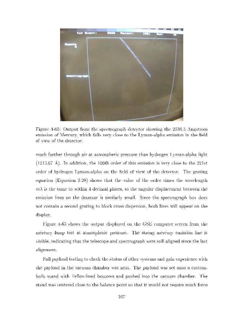
Figure 4-65: Output from the spectrograph detector showing the 2536.5 Angstromemission of Mercury, which falls very close to the Lyman-alpha emission in the eldof view of the detector.
much further through air at atmospheric pressure than hydrogen Lyman-alpha light
(1215.67 Å). In addition, the 106th order of this emission is very close to the 221st
order of hydrogen Lyman-alpha on the eld of view of the detector. The grating
equation (Equation 2.28) shows that the value of the order times the wavelength
mλ is the same to within 4 decimal places, so the angular displacement between the
emission lines on the detector is similarly small. Since the spectrograph box does
not contain a second grating to block cross dispersion, both lines will appear on the
display.
Figure 4-65 shows the output displayed on the GSE computer screen from the
mercury lamp test at atmospheric pressure. The strong mercury emission line is
visible, indicating that the telescope and spectrograph were still aligned since the last
alignment.
Full payload testing to check the status of other systems and gain experience with
the payload in the vacuum chamber was next. The payload was set onto a custom-
built stand with Teon-lined bottoms and pushed into the vacuum chamber. The
stand was centered close to the balance point so that it would not require much force
167

Figure 4-66: Full payload inside the VACTEF vacuum chamber ready for testing.
on the back of the payload to tip the telescope downward. An accordion table was
placed beneath the end of the payload to carefully adjust the tilt of the telescope. The
spaghetti box containing the WFF-93 PCM (see Section 4.2.6) was also placed in
the vacuum chamber with the payload, and all the wiring to the outside was connected
through a feedthrough plate near the door of the vacuum chamber. Figure 4-66 shows
the testing setup as viewed from the primary vacuum chamber door.
The light source chamber was not congured with the collimating mirror setup to
produce collimated light to properly test the optics, so a temporary setup was built
to supply mechanically-collimated light into the chamber. At the end of the chamber
where the light source is located, a at plate with a small hole was designed, built,
and installed so that only a small amount of light could exit the light source chamber.
A stand was designed and built to mount existing pinholes that allowed even less light
from the light source chamber through to the telescope. This stand was placed in
168

Figure 4-67: Plate with small hole at the back end of the VACTEF vacuum chamber(left), and a stand for mounting pinholes and blocking stray light from entering thetelescope (right).
front of the telescope and eectively prevented stray light from entering the telescope
while being nearly collimated at short distances. Figure 4-67 shows the plate at the
back wall of the chamber and the stand to mount the existing pinholes in.
To ensure that this mechanical collimator setup was working and that no stray
light was entering the system, it was tested with visible light at atmospheric pressure
using the Xybion camera for feedback. The telescope was rotated from left to right
inside the chamber. Each time the payload reached the limit of horizontal motion,
the accordion table was raised higher so the telescope pointed lower. This back-and-
forth, up-and-down maneuver covered the entire pointing range of the payload inside
the vacuum chamber. The only time light was seen in the Xybion camera's eld of
view was when it was pointed directly at the pinhole on the stand set up near the
center of the chamber, which meant that there was not a signicant amount of stray
light reecting o the walls of the chamber and entering the telescope.
Figure 4-68 shows the video feed from the Xybion camera during this test. The
view is partially obstructed because wires had to be rerouted through the large hole
in the visible optics board so the spectrograph detector could be connected to the
imager charge amps. This problem had not been considered before alignment but
169

Figure 4-68: Xybion camera output during testing at atmospheric pressure with vis-ible light.
did not need to be xed to show that the camera and mechanical collimator were
working.
Finally, the full payload was tested at vacuum. The visible light source mounted
in the light source chamber was replaced with a deuterium lamp. All systems were
powered down while the pressure in the vacuum chamber descended below 10-6 Torr.
When the deuterium lamp was turned on and the detectors were powered up, a
Lyman-alpha emission was visible on the GSE computer screen. This also conrmed
that the Xybion camera and the spectrograph box were in alignment relative to each
other.
This vacuum test did not assess the performance on the SPACOM star tracker or
the imager detector, nor did it allow the team to calculate a total eciency of the
optics and spectrograph detector. Once the payload was removed from the vacuum
chamber, it was disassembled so each section could be calibrated. The telescope was
relatively calibrated with a photomultiplier tube (PMT) in the VACTEF vacuum
chamber before the rest of the optics and the PMT were absolutely calibrated with a
photodiode in the VUCL.
170

4.5.2 Calibrating the Telescope
The reectivity of the telescope was calibrated using the PMT. This instrument had
not been absolutely calibrated yet, but all that was required to determine reectivity
of the telescope mirrors was a relative calibration. The telescope section and center
plate were removed from the rest of the payload and placed in the vacuum chamber
with no electronic equipment other than the PMT.
First, the deuterium lamp's output was monitored over time. The photomultiplier
tube was set on the accordion stand behind the pinhole holder plate. Visible light was
used to align the face of the PMT with the beam of light going through the pinhole.
The visible light bulb was replaced with the deuterium lamp and the chamber was
brought to vacuum. The deuterium lamp only can be turned on and o; its output is
not adjustable but this test showed that the output varies by a few percent over the
course of an hour. The results from this test are available in the attached Appendix
DVD.
Next, the PMT was moved behind the telescope. Light now passed through the
pinhole stand, through the telescope, and hit the PMT. Alignment was checked using
visible light before mounting the deuterium lamp and bringing the entire system down
to vacuum. After a test, the telescope was rotated 120 degrees so that one relative
calibration was done in each of the three sections of the telescope.
The results show that the telescope is not uniformly reective. One section had an
overall reectivity near 20%, which is much less than what the reectivity would be
with two aluminum mirrors with fresh magnesium uoride coating. Another section
had a total reectivity near 12%, which is a 60% dierence in total reectivity. An
eciency degradation of this magnitude would cause the VeSpR mission to fail, and
most likely does account for the unexpected loss of overall eciency that JASpR ex-
perienced. In addition, the non-uniform degradation is consistent with the possibility
that the mirrors were contaminated by oil from a diusion pump used in the vacuum
chamber at WFF that entered the vacuum system due to improper operation of the
system. The full results from mirror testing are available in the attached Appendix
171

DVD.
4.5.3 Calibrating the Detectors and Windows
After initial full payload testing, the experiment team moved the structure of the
payload from the basement VACTEF to the 5th oor VUCL. This was easier than
separating out the control electronics in the GSE and taking only the detectors and
optics that would be tested individually. Before testing in the vacuum chamber could
begin, new test wiring harnesses had to be fabricated to connect all of the electronics
as if they were assembled inside the payload, even though pieces of the system were
inside the vacuum chamber.
Testing inside the vacuum chamber required that a detector subsystem (see Figure
4-29), its charge amps, its high voltage power supply, and the VIP high voltage power
supply be inside the vacuum chamber. The charge amps must be inside the vacuum
chamber with the detector because cables running from the detector to the charge
amps must be shorter than 12 inches. If extended cables were used to route signals
outside of the vacuum chamber, line losses would make the signal unreadable. The
high voltage power supplies needed to be inside the chamber because there are no
high voltage transmission lines through the electrical feedthrough plate (see Figure
4-57(left)) and because transmitting high voltage through a vacuum wall can be
dangerous. Wiring harnesses were fabricated to connect the power inputs and data
outputs on the payload outside the vacuum chamber to the electrical feedthrough
plate and to connect the feedthrough plate to the payload components inside the
vacuum chamber.
The VUCL has an absolutely calibrated photodiode that was used for absolute
calibrations. The photodiode is attached to a lever that can be rotated from outside
of the vacuum chamber so it can be moved into place to capture light from the
monochromator and then moved out of the way so the test optics can be calibrated.
There is also a mesh diuser installed on the same lever that has a 1.33% throughput.
In addition, the optics table inside the chamber can be translated and rotated to
dierent positions while the chamber is at vacuum.
172

First, the PMT was absolutely calibrated with the photodiode. The PMT was
set on the optics table inside the vacuum chamber and a green laser was used to
align the front face with the beam path from the monochromator. The chamber was
pumped down, the monochromator was powered on, and measurements from both
the photodiode and the PMT were taken. At Lyman-alpha, the PMT has a quantum
eciency of 2.46%±0.16%.
Next, the spectrograph MCP detector was calibrated. The PMT and detector were
set up side by side at the same height on the optics table. Both were aligned with
the green laser. Once one was aligned, the table was moved by a known distance and
the other was aligned. The table was moved back and forth several times to ensure
the instruments were still aligned with the beam path even after the table moved
(due to problems described in Section 4.3, this caused the longer delays in testing)
Next, the chamber was sealed and brought down to vacuum and the monochromator
and instruments were powered on. Measurements were taken with one instrument
before the table was moved so that measurements could be taken with the other. At
Lyman-alpha, the MCP detector has a quantum eciency of 12.22%±0.46%. This
is a weighted average of four measurements and the relative error is 3.80% (relative
error is the standard deviation divided by the mean) [54].
To test the throughput eciency of the magnesium uoride windows of the detec-
tors, the window on the imager detector was taken o the detector housing. A similar
setup to the detector calibration was used for the window calibration except the sec-
ond window was placed in front of the detector. At Lyman-alpha, the magnesium
uoride windows had a throughput eciency of 26.0%±2.02%. This is a weighted
average of two measurements and the relative error is 7.78%. The raw data for all
the results discussed in this section are available in the attached Appendix DVD.
It would be easy to assume that because the window's throughput eciency is
roughly 25%, the quantum eciency of the detector should be four times higher than
reported. However, the magnesium uoride windows should have much higher overall
throughput eciency, closer to 50%. At the time of testing, the team was unable
to switch out the windows, recalibrate the detector with the imager window, and
173

calibrate the spectrograph detector's window to determine if both had both had been
equally contaminated.
4.5.4 Calibrating the Spectrograph Box
The spectrograph is the primary scientic payload on VeSpR. Ensuring that it is
aligned properly and has maximum throughput is vital to the success of the mission.
Having an absolute calibration of the instrument is vital to proper data reduction. Too
low of a throughput in the instrument would result in high error in the measurement
of D/H in Venus' atmosphere (see Section 5.5).
The detector was mounted back on the spectrograph box and baes were secured
to both sides of the light entrance hole. The box was placed next to the PMT on the
optics table. A green laser was used to align both instruments with the moving optics
table. Alignment of the spectrograph box was especially dicult, not only because of
the size of the box but also because of the precision required. The box was aligned so
that the laser beam was centered at ends of both baes. Because the echelle grating
does not disperse green light into the same locations it disperses Lyman-alpha light,
it was impossible to check that light would enter the detector with the laser beam.
The angle of the echelle grating was changed by small amounts using 0.5 mm
shims stacked beneath the grating. Several tests were performed at dierent angles
to ensure that the 221st order of Lyman-alpha was centered on the detector. This
was painstakingly checked by bringing the chamber to vacuum, powering on the
monochromator, testing the brightness measured on the PMT compared to the MCP
detector, and bringing the whole system back up to air to try a dierent angle.
Because of the system leaks, table jamming problems, and the accidental rotation of
the screws the echelle grating rests on, this process took weeks of vacuum chamber
time.
Once the team had centered the 221st order on the detector, the nal calibration
was made. At Lyman-alpha, the spectrograph box optics have a total reective
eciency of 11.47%±0.52%. This is a weighted average of three measurements and
the relative error is 4.52%. This is a good throughput; if the parabolic mirror has
174

a reective eciency of 75% at Lyman-alpha, this means the echelle grating has
a grating eciency near 20%. Both of those numbers are close to their maximum
theoretical values.
After all the tests described in this section were completed, the mirrors were sent
to Goddard Space Flight Center (GSFC) to be recoated. This process would bring
the eciencies back to their maximum theoretical eciencies at Lyman-alpha, which
is close to 80%. Once the mirrors were returned to the facilities at BU, they were left
in the shipping containers to protect them from dust, humidity, and other airborne
contaminants until all other design changes had been nished.
The echelle grating, the MCP detectors, and the magnesium uoride detector
windows stayed at BU. The windows were carefully cleaned with isopropanol and a
Q-tip. There are multiple spare windows that were not tested, so when the payload
is reassembled, all the windows will be tested and the two windows with the highest
throughput will be used. Now that the operating performance of the payload had
been characterized, it was time to determine what design aspects needed to change
in order for the mission to be successful.
175

176

Chapter 5
Refurbishing The Venus Spectral
Rocket
5.1 Tracking Cascading Design Changes
A system engineer does not specialize in designing or understanding every component
in every subsystem on a spacecraft. A systems engineer specializes in understanding
the relationships between subsystems, the design parameter space, and especially
how changes in one subsystem can cascade and cause changes in other subsystems.
In testing and preparing the VeSpR hardware for its rst ight in over a decade, many
design changes had to occur, which caused cascades of other changes. This section
explains the top level design changes that caused many other subsystem changes
throughout the entire payload and forced new subsystem requirements to be written
and satised.
5.1.1 Changes Due to Upgrading the Detectors
Initial calibration testing (Section 4.5) showed that the Wedge-Strip-Zigzag (WSZ)
detectors used in the JASpR payload since 1993 had low quantum eciency com-
pared to previous calibrations. This quantum eciency would not be high enough to
properly meet the primary science objective to measure the D/H ratio in the upper
177

atmosphere of Venus. The detectors needed to be refurbished to have better quantum
eciency or be replaced with new ones.
The VeSpR Principal Investigator has a long history of working with Sensor Sci-
ences, a company based in Berkeley, California that developed and delivered the WSZ
detectors in 1993 along with the charge ampliers and analog-to-digital converters
(ADC). However, because the WSZ detectors were so old, the equipment required to
refurbish the detectors had not been used in a long time. Sensor Science engineers
informed the payload team that refurbishing the old detectors would cost even more
than purchasing new ones. In addition, Sensor Sciences expressed concern regarding
the reliability of the detectors because they were so old.
Over the past two decades, ultraviolet detector technology has greatly improved.
Sensor Sciences has been manufacturing a newer type of detector called the Cross-
Delay Line (XDL) detector (see Section 2.7). New XDL detectors have higher quan-
tum eciency and are more reliable compared to refurbished WSZ detectors. In the
end, the advantages of having the new XDL detectors outweighed the option to use
the original WSZ detectors and pay the high cost of refurbishment.
However, this single top-level (Level 1) design change created the largest cascade
of lower-level changes of all the other top-level design changes. As a result, VeSpR is
signicantly dierent than JASpR in terms of raw capability, internal part placement,
and subsystems components. Figure 5-1 shows a summary of the cascade of design
changes that occurred because of this single design change.
Since the XDL detectors have an entirely dierent output than the WSZ detec-
tors, the Level 2 design changes involved new electronics for receiving data from the
detectors. The original ADCs and charge ampliers needed to be replaced with new
ones. Since the XDL measures a time delay to get a reading of position, the elec-
tronics require a time-to-digital converter (TDC) instead of an ADC. The XDL also
only requires one charge amplier that can receive all of the necessary outputs of the
detector compared to the three ampliers needed for the three signals coming from
the WSZ detector. All of these ampliers also came from Sensor Sciences.
The XDL detectors also have dierent power requirements than the WSZ detec-
178
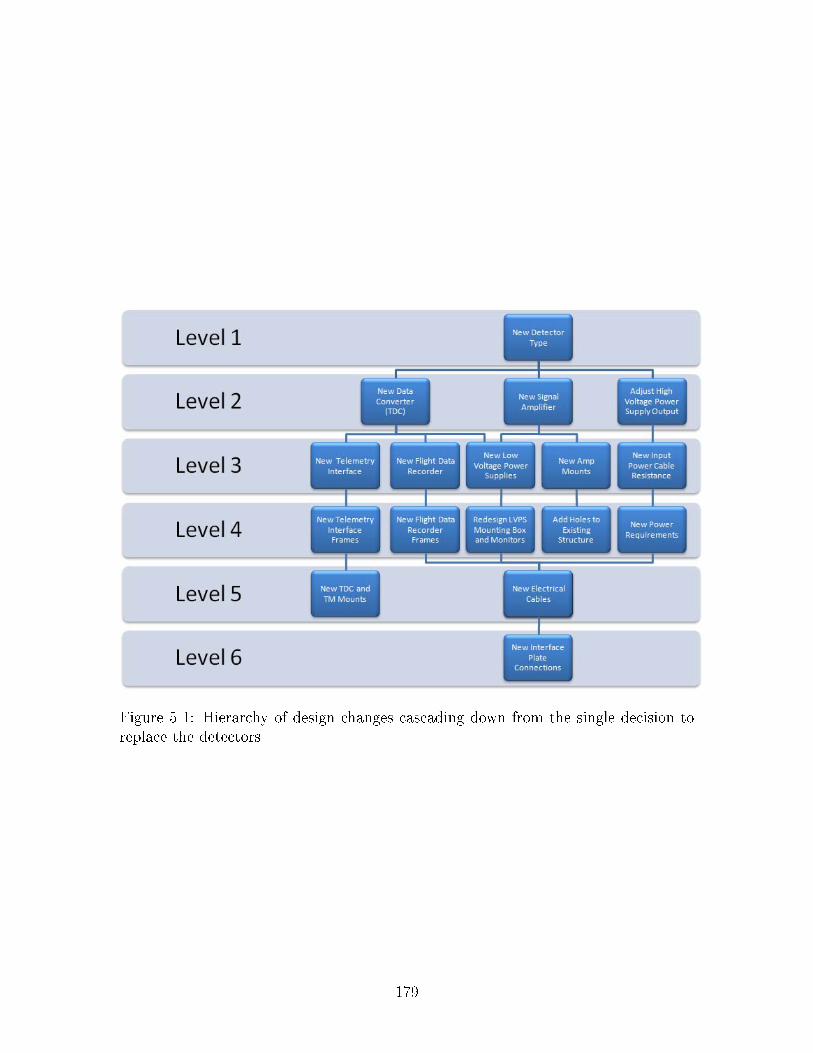
Figure 5-1: Hierarchy of design changes cascading down from the single decision toreplace the detectors
179
tors. Both need high negative voltage to operate, but WSZ detectors required 4.5
kV whereas the XDL detectors require -5 kV. The SPACOM high voltage power sup-
plies that were used to power the WSZ detectors had the capability to power the
XDL detectors, but the output voltage needed to be changed. The SPACOM's high
voltage output can be tuned by changing the programming resistor that connects
into the 9-pin D-sub connector that also provides the input power. This required
careful testing to ensure that the output was tuned to the proper voltage within an
acceptable error level. The Level 2 change of tuning the voltage created a Level 3
change of replacing the connector that housed the original tuning resistor.
The charge ampliers for the XDL detector have a dierent shape than the charge
ampliers for the WSZ detector, so the XDL ampliers cannot go in the same locations
inside the payload. Sections of the payload were specially carved out of the structural
plates to support the original amps, but the new ones would not t in those locations.
A Level 3 design change was to redesign the plate that both amps securely mounted
to, and a Level 4 change was to modify the existing structure so that the plate could
be mounted so as to survive the stresses and vibrations of ight (Section 5.3.5).
Because the XDL detector's TDC outputs a completely dierent type of signal
than the WSZ detector's ADC, a new telemetry interface had to be designed to feed
digital signals into the WFF Pulse Code Modulator 93 (PCM-93) parallel port, and a
new backup ight data recorder (FDR) had to be designed in the event of a telemetry
failure during the ight, creating two more Level 3 changes. One of the telemetry
interfaces and the original ight computer were non-functional already (Section 4.4),
and since the nal JASpR ight Wallops had upgraded to a new telemetry system
entirely (see Section 5.1.4), so redesigning the interfaces and designing a new FDR
was already being considered during early preparations for ight. Both of these
components were developed by the electrical and computer engineers at the MIT
Kavli Institute rather than the primary payload scientists and engineers working at
Boston University.
The combination of new TDCs, new charge ampliers, new TM interfaces, and
new FDRs brought new power requirements that forced a Level 3 design change in the
180

low voltage power supply system that powered the original electronics. The original
ADC and charge ampliers required ±12 V and +5 V inputs, whereas the new TDCs
and charge ampliers required ±12 V and ±6 V. Since the new power supplies had to
be integrated into the existing structure, this created Level 4 design changes in the
low voltage power supply housing box (see Section 5.2.4).
New TM interface and FDR electronics required new frames to support these
electronics, both of which were Level 4 changes. The FDR and its frame were designed
to be mounted into the same location as the original ight computer (see Section
5.3.3), so no further changes were needed to secure it in the payload. The TM
interfaces were designed to mount on the TDCs in the same way that the original
TM interfaces mounted to the ADCs on the sides of the spectrograph box (see Section
5.3.4), but since the TDCs have dierent dimensions than the ADCs, a new mounting
plate had to be designed, extending the cascading design change tree down to Level
5.
Another Level 5 design change was redesigning the wiring harnesses that connected
and powered all of the electronic components. All of the new components required
new cable pinouts, which needed careful planning and documentation so they could
be manufactured by the MIT Kavli Institute electrical engineers. These cable changes
then forced a Level 6 design change, a redesign of the Interface Plate to the Wallops
Attitude Control System (ACS) (see Section 5.3.8).
Luckily, a major Level 2 design change was avoided by the fact that the payload
team was able to reuse the original detector housings with the new detectors. If en-
tirely new housings had to be built, there would have been a cascade of major changes
to many elements of the payload, including the detector mounts in the optics, the
vacuum ion pump (VIP) connections to the detector housings, and the VIP mounts
in the payload. Because the same housings are being reused, the only other Level 2
change needed was to design a new back plate that seals the detector in the housing
and has the proper terminals to send data to the charge amps (not shown in Figure
5-1).
181
5.1.2 Changes Due to Wallops ACS Rail Position
While the VeSpR/JASpR payload had not changed much in the previous decade,
the ACS system developed by Wallops Flight Facility that was going to be used
on the VeSpR ight certainly had. One of the seemingly minor changes was the
position of the launch rail with respect to the payload. While the telescope section
of the payload has rotational symmetry, the rest of the payload, specically the star
tracker and interface plate, does not. Because of the small rotation in the launch rail's
location, design changes needed to occur for VeSpR to work with the new systems. In
addition, the telemetry channels that originally read the analog output from the star
tracker placed in the telescope are obsolete and are not in the current ACS platform
Wallops uses.
When the payload team was informed of the rail position change relative to the
original zero degree marker from JASpR ights, the payload was in many pieces and
needed to be partially reassembled before the exact dierence between the zero degree
line as dened by Wallops and the zero degree line as dened by the coordinate system
of the star tracker could be measured. After pouring through old photographs and
struggling to reassemble sections without parts that were either being tested, being
replaced, or being refurbished, the payload team was able to back out the dierence
between the zero degree lines and measure a 15-degree dierence between the new
rail placement and the spectrograph aperture.
Initially, the Wallops ACS engineers wanted to rotate the star tracker within
the payload to match the orientation of the rail, but this option was very quickly
ruled out by the Principal Investigator because the incredible precision needed and
already achieved in the optics system would be costly and risky to modify. Instead,
Wallops decided to change the hardware programming and manually convert X and
Y coordinate positioning signals before streaming them through the telemetry. This
way, there is no dierence between the rail and the star tracker as seen during ight
on the ground if a human operator needs to take control in the event of a positioning
failure and has to rely on the payload's star tracker for guidance.
182

However, Wallops ACS engineers wanted the analog signals from the star tracker
to be converted to RS-422 signals before exiting the payload, rather than nding
another way to accept the analog signals in the ACS section. This required a Level 2
change to the payload to have an analog-to-RS-422 converter designed and installed
inside the payload (Section 5.2.3). The RS-422 converter was also designed by the
MIT Kavli Institute electrical and computer engineers. This new electronic board
created Level 3 design changes, such as the need for a frame to mount the board in
and revised power requirements, which then created Level 4 design changes in the
wiring harnesses and the interface plate to connect with the Wallops ACS.
Another change in the Wallops ACS from the previous JASpR ight was that the
standard bus for the ACS appears to have been rotated relative to its past position.
The original placement of the connectors on the interface plate, shown in Figure 5-
2, appears to have been inuenced by the ACS architecture immediately forward of
the interface plate. The connectors are all placed within the half-circle from ~300
degrees to ~120 degrees relative to the original zero degree rail marker (circled in red
on Figure 5-2), meaning the inside components of the ACS came down closer to the
payload on the other half of the interface plate.
However, after a Wallops mechanical engineer noted the rail placement as it was
on JASpR, he informed the payload team that the connectors would have to move
because the new ACS had components occupying space from 270 to 90 degrees relative
to the rail, or Quadrants 1 and 2 of the coordinate frame shown in Figure 5-3. VeSpR
connectors had to be moved to Quadrants 3 and 4 to avoid interfering with those
systems, shown from a side view in Figure 5-4.
The unexpected ACS repositioning Level 1 change caused Level 2 changes of
moving those connectors to the lower half of the coordinate frame. This was not easy,
but a positioning frame was found that did not require any cables that were being
reused or changed to be cut, lengthened, or altered in any way. Some of the other
cables that were already being changed needed to be rerouted from their original
positions, but luckily these Level 3 design changes were small and were made long
before those cables were constructed.
183

Figure 5-2: View of the JASpR Interface Plate looking toward the tail of the rocket.Previous zero degree line relative to rail marked with R (circled in red)
Figure 5-3: View of the ACS system looking toward the nosecone of the rocket
184

Figure 5-4: View of the ACS looking sideways
5.1.3 Changes Due to Increased Pointing Accuracy
One of the advantages that the VeSpR ACS has over earlier JASpR ights is improved
pointing accuracy and control. The secondary mirror of the JASpR telescope was
automatically controlled by tip/tilt servos that received error signals from the star
tracker to compensate for pointing drift. Since the last JASpR ight, one of the
two servos burned out and does not work. Even though it is possible to perform
spectroscopy with only one servo, these moving parts and the feedback loop between
the star tracker and the servos were potential failure modes that could cause a mission
failure.
Since the previous JASpR ight, the ACS pointing accuracy has increased enough
that pointing accuracy controlled by the secondary mirror is no longer needed. As
a consequence, a Level 2 design change was to remove the active tip/tilt stage on
the secondary mirror and replace it with a passive, securely aligned system, which
removed this potentially hazardous failure mode (see Section 5.3.6).
The star tracker would continue to be used in operation; however, instead of being
185

transmitted to components within the payload, signals from the star tracker would
only be sent to the ACS. The ST-5000 Wallops star tracker mounted in front of the
telescope mirror section is programmed to specically ignore planets, and because
VeSpR will be pointing very close to the sunlit horizon, there might not be enough
stars in the eld of view to our pointing needs. However, the star tracker mounted
inside the payload not only has the same eld of view as the other scientic instru-
ments, it can transmit signals that help determine exactly how far away from the
center of the planet VeSpR is pointing. Using these signals, the ACS can properly
maintain its lock on targets during the mission. Removing old, complex wiring and
control boxes for the servos and replacing them with one wiring harness connected
directly to the ACS was a welcome and easy Level 3 design change.
5.1.4 Changes Due to Updated Telemetry Requirements
Another overall improvement in the Wallops ACS since the last JASpR ight was
an increase in the rate that data could be transmitted. When the telemetry inter-
faces were designed in the early 1990's, the telemetry rate was only 1 Mbps. As a
consequence of that constraint, the telemetry interfaces were only designed to send
out 2,500 counts of data per second. This was not considered a problem, especially
considering that the WSZ detectors could only process approximately 5,000 counts
per second before dead time eects started degrading quality of the data, and JASpR
never viewed targets that produced much more than 1,500 counts per second anyway.
Today, the Wallops ACS uses a 10 Mbps data rate. This order of magnitude
increase in available data to stream, compounded by the fact that the XDL detectors
can handle 100,000 counts per second with 10% dead time, the payload team decided
that the maximum detector count rate through the telemetry stream should be 25,000
counts per second. This order of magnitude increase was also justied by the mission's
target selection; during the nal seconds above 110 km, VeSpR will observe the sunlit
Moon for an additional in-ight calibration, and the spectrograph detector may detect
count rates as high as 20,000 counts per second.
The increased telemetry capabilities and the scientic desire to follow suit with
186

VeSpR's data stream drove the design requirements for the telemetry interface and
FDR. While this may not be considered much of a cascade of design changes since
the design had not been made, this case still illustrates an example of how customers'
desires can form the top level requirements that drive the systems engineering ap-
proach to designing spacecraft.
5.1.5 Combined Changes and Other Design Constraints
Lower level design changes do not necessarily have only one parent Level 1 design
change. Many of the lower level design changes had to be made while considering
requirements driven from many higher level changes. For instance, the Interface Plate
needed Level 6 changes because of the new detectors, but Wallops needed dierent
connector types altogether for many of their connections, which were Level 1 changes.
The low voltage power supply also had a variety of parent constraints at dierent
levels.
Unfortunately, the entire scope of all the design changes required and the con-
straints between all of the working parts was not well known when the refurbishment
work was beginning. While each design choice was made to optimize a given set of
constraints for each part designed or modied, the global sum of all the design changes
is suboptimal in terms of cost and overall performance because not all of the require-
ments were known well enough in advance. In some cases, constraints added at later
times continued to cascade, causing some design decisions, which were thought to be
optimal locally, to be suboptimal globally and perhaps more costly than necessary.
One of the major drivers for design constraints was the desire to reuse parts that
had already own on the rocket, not only to avoid further materials, machining, and
design costs but also to keep the payload similar enough to its previous ight that
it could still be considered a reight to avoid having to get a complete payload
certication again. However, in many instances, dropping a cheap constraint (like
not reusing existing holes and drilling new ones) drove costs higher in the end. These
cases as seen in hindsight will be discussed where appropriate in Sections 5.2 and 5.3.
187

5.2 Designing Payload Electrical Components
The science team at BU does not have the expertise to design all of the new elec-
tronic components, so engineers at the MIT Kavli Institute were contracted to design
and build the electronics discussed in this section. The science team was primarily
responsible for communicating needs, writing requirements, designing the structural
housings (see Section 5.3), and testing the nal products. The science team worked
closely with the Kavli engineers to ensure that the nal products were what the VeSpR
payload needed.
Many of the requirements for these systems were driven by the characteristics of
the new TDCs and charge ampliers that operated with the new XDL MCP detectors.
The old ADCs and charge ampliers used +5 V and ±12 V power inputs, but the
new TDCs and charge ampliers require ±6 V and ±12 V. For this reason, many of
the following components were designed to operate with a +6 V input power rather
than the standard +5 V that most digital systems use.
5.2.1 Telemetry Interfaces
Since the original Spectrograph TM Interface had burned out, the science team knew
from the beginning that the TM Interfaces needed to be redesigned. The new detector
data outputs and new Wallops telemetry requirements also served as constraints in
the design of the new interfaces. The primary function of the TM Interfaces is to
take data from the TDCs, convert it to parallel data, and send it to the Telemetry
Section and to the ight computer.
The TM Interface was designed to accept the three sets of signals coming from
three 25-pin connectors on the TDC corresponding to X, Y, and P data. X and Y
data correspond to the x- and y-positioning of photon counts on the detector while
the P data corresponds to pulse height. The TM Interface outputs a 32-bit parallel
word that is read by the Telemetry section. The data is also sent to the FDR as two
16-bit words that sync with the Telemetry section.
Due to ITAR restrictions, more details on the design and function of the TM
188

Interface are not being published here. More information on the output from the
detectors is available on the attached Appendix DVD.
5.2.2 Flight Data Recorders
The original ight computer was inoperable from the beginning of the project and
needed to be removed from the payload. Even though there is no need to control any
systems using a ight computer in the payload, there was still a strong desire to have
a backup computer recording data from the detectors.
Before choosing a design conguration, the ight data recorder (FDR) require-
ments were considered. The computer needed to boot up quickly because once power
was turned on to the payload, data would start coming in from the detectors that
needed to be recorded, and many computer modules have startup times that can be
as long as 30 seconds. The computer also needed to be fast enough to record data
at the maximum telemetry rate, 25 kHz, but most processors can handle that speed
nowadays. The science team would need to retrieve the data easily while the science
payload was connected to the rest of the payload during integration testing, so there
needed to be a way to do this. The computer would also need to be small enough to
t inside the payload, preferably near the location of the old ight computer.
Initially, the team looked into the components needed to build a custom module,
but the Kavli engineers found a commercially available module that would be able
to satisfy all of our requirements. The TS-7400 is an embedded computer system
module with a 200 MHz ARM9 processor that requires less than 3 Watts of power.
It can write data to a standard-capacity SD card and uses USB or Ethernet cables
to communicate with other computers. It only takes up 2.9 x 4.7 x 1.5 in of space
within a frame and easily ts within the footprint of the old ight computer. Figure
5-5 shows a picture of the TS-7400 module taken from the product manual.
The module requires +5 V power to operate, but since the NLVPS was losing its
+5 V power supply module, the Kavli engineers found a way to route power that is
stepped down from +6 V to +5 V to the FDR through the TM Interface. This has
the advantage that only one cable is needed to support the FDR that carries power
189

Figure 5-5: Layout of TS-7400 computer module taken from product manual.
and data. The other option would be to take +5 V power from the OLVPS, but
that would require new cables routing through J20 and much more rewiring through
the top section of the payload with no guarantee that the ±5 V supply module in
the OLVPS can even output enough current since there are no longer any product
specications for that module.
During ight, the science payload will be powered on after the entire payload is
above 110 km. The Kavli engineers have programmed the FDR to boot up once power
is turned on. Boot up time is 1.1 seconds, and a new le is automatically written
on the SD card and data from the TM Interface is written to that le after boot up.
Since the telescope will not have even pointed to the rst target, these 1.1 seconds of
data that are lost is inconsequential to the mission outcome.
Because the FDR is only a backup data recording system, it is designed to be
passive. It does not send any signals to the TM Interface; instead, the TM Interface
automatically supplies data when the Telemetry Section signals the data on the TM
Interface to be supplied. This way, a failure of the FDR does not aect the operation
of the TM Interface, which is a vital component to the experiment.
190

Figure 5-6: Silkscreen schematic of the RS-422 Converter.
5.2.3 RS-422 Converter
The SPACOM star tracker that was used to adjust the secondary mirror positioning
uses a quadrant photodiode to measure the pointing accuracy of the telescope to
within 1 arcsec. Since the pointing accuracy of the entire payload is within±1.5 arcsec
and the secondary mirror positioning system was being taken out, WFF wanted to
use the error signals from this instrument as a backup to obtain an even ner pointing
accuracy.
However, the SPACOM star tracker outputs analog signals and WFF wanted sig-
nals converted to a specic RS-422 format before they entered the telemetry stream.
The MIT Kavli engineers designed the board that would perform this task. A
silkscreen of the board is shown in Figure 5-6.
The board was designed to operate with +6V input power. The science team
191

Table 5.1: Power Requirements for new low voltage systems powered by the New LowVoltage Power Supply (NLVPS) box.
Part Qty +6V(mA) -6V(mA) 6V(W) +12V(mA) -12V(mA) 12V(W)Amplier 2 0 0 0 146 36 2.73TDC 2 430 730 6.96 47 83 1.56
Interface 2 0.25 0 1 0 0 0FDR 2 500 0 3 0 0 0RS-422 1 0.25 0 1 0 0 0Total 1860.75 1460 22.92 386 238 8.58
worked closely with WFF engineers and the Kavli engineers to ensure that the signals
coming out of the board were to specication. However, because of ITAR restrictions,
the nature of this output signal will not be discussed.
5.2.4 New Low Voltage Power Supply Box
Since most of the electronics that the New Low Voltage Power Supply (NLVPS) sup-
plied power to were replaced, it had to be redesigned to satisfy the power requirements
of the new electronics, shown in Table 5.1. Redesigning this component was more
of a systems engineering challenge than an electrical engineering challenge because
of all the requirements this component needs to satisfy. Not only must it be able to
produce the correct voltages and supply the necessary power, but careful planning
was needed to ensure that the wiring required to supply all of these components was
possible and would not interfere with any other payload components.
The EMI lter module and the±12 V power supply module, both manufactured by
Interpoint, were both still in working condition and were able to be reused. Interpoint
only had one module that was capable of producing ±6 V, and its maximum power
output of 120 W greatly exceeds the requirements of the system. However, the module
is spaceight qualied, and the team was not able to nd a similar component from
a competing manufacturer, so the Interpoint module was used in the design.
The box that housed the power supply modules needed to be modied because the
±6 V supply was not the same size as the other modules. In addition, there needed
to be space for a new 9-pin connector to power the RS-422 converter. Appropriate
192
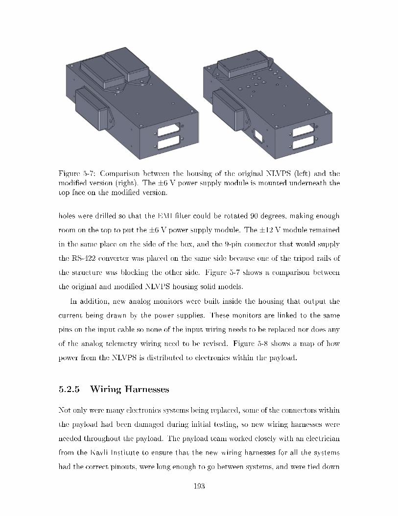
Figure 5-7: Comparison between the housing of the original NLVPS (left) and themodied version (right). The ±6 V power supply module is mounted underneath thetop face on the modied version.
holes were drilled so that the EMI lter could be rotated 90 degrees, making enough
room on the top to put the ±6 V power supply module. The ±12 V module remained
in the same place on the side of the box, and the 9-pin connector that would supply
the RS-422 converter was placed on the same side because one of the tripod rails of
the structure was blocking the other side. Figure 5-7 shows a comparison between
the original and modied NLVPS housing solid models.
In addition, new analog monitors were built inside the housing that output the
current being drawn by the power supplies. These monitors are linked to the same
pins on the input cable so none of the input wiring needs to be replaced nor does any
of the analog telemetry wiring need to be revised. Figure 5-8 shows a map of how
power from the NLVPS is distributed to electronics within the payload.
5.2.5 Wiring Harnesses
Not only were many electronics systems being replaced, some of the connectors within
the payload had been damaged during initial testing, so new wiring harnesses were
needed throughout the payload. The payload team worked closely with an electrician
from the Kavli Institute to ensure that the new wiring harnesses for all the systems
had the correct pinouts, were long enough to go between systems, and were tied down
193

Figure 5-8: Updated New Low Voltage Power Supply (NLVPS) schematic.
tightly enough to prevent vibration stress from damaging the connectors. Although
the team fabricated all of their own harnesses for laboratory testing, only the Kavli
electrician fabricated harnesses that went into the payload.
After the initial autopsy of the payload, the wiring documentation for the entire
payload was digitized and put into a format that the team could edit. As changes
were being made throughout the system, pages in the wiring notebook were updated.
The Interface Plate's interface control document was also updated as decisions were
nalized, and the electrical engineers at WFF were questioned before changes were
made to the document to ensure systems would still be compatible and given the
revised document after the changes were documented. Due to ITAR restrictions, the
wiring notebook cannot be made publicly available.
5.3 Designing Payload Mechanical Components
Many of the design changes made to VeSpR during the process of preparing the
payload for re-ight were intended to keep the payload as similar to the 13.174 JASpR
194

V ight as possible to avoid full-payload structural vibration testing during payload
integration. Structural vibration testing puts more vibration stress on the payload
than the actual ight does, and the Principal Investigator feared that full payload
vibration testing could irreparably and needlessly damage the optics.
Great strides were made to position new components in nearly the same locations
as they originally were. All new components will undergo individual part vibration
testing to ensure they are capable of surviving the launch loads, but with luck the
entire payload will not need to be structurally tested.
Since the payload and its new components are being tested in vacuum chambers,
many design considerations are shared throughout the payload and its new compo-
nents. One of the major challenges was ensuring that no threaded hole was unvented
or otherwise blocked o. This can create a pocket of air that slowly leaks out into
the vacuum chamber. These virtual leaks keep the air pressure inside the vacuum
chamber higher than desired, which makes pumping down the pressure to adequate
levels for ultraviolet testing take much more time. It can also lead to absorption of
ultraviolet light in ight. Avoiding virtual leaks was a major challenge in the design
of the TM, RS-422, and FDR frames.
In addition, many other subtle design constraints are reected throughout the
design of the following components. For instance, all inner corners of spaces such as
D-subminiature connector holes had to be rounded; it is impossible to cut a square
hole with a round milling bit. Threaded holes were checked to make sure there are at
least four threads per screw. Counter-sinks have tolerances specied to make sure the
screw heads are below the surface they share with the part. All mechanical design
work was done in SolidWorks. The Boston University Scientic Instruments Facility
was contracted to perform most of the machining work, with minor machining done
by the experiment team at the MIT Aeronautics and Astronautics machine shop.
5.3.1 Telemetry Interface Frames
The frames to house the new telemetry interfaces were the rst components to be
designed and machined. The JASpR TM interfaces and ADCs were identical in size
195

Figure 5-9: Machinist drawing (left) and solid model (right) of the TDC
and mounted on the broad sides of the spectrograph box. This space was adequate
to mount the new TDCs and TM interfaces. The TDCs are slightly bigger than the
ADCs (10.275 x 8.090 x 1.073 in), and the TM interface was expected not to need
nearly as much space, so the TM interface board was sized so it would t in a frame
with a footprint half the size of the TDC. The TM interface and TDC would share
the same mounting holes, the three on the bottom near the charge amplier inputs
and the two in the center. The TDC inputs would face the telescope section, which
is aft to the whole rocket, and the outputs would face the ACS and nosecone. Figure
5-9 shows the machinist drawing and solid model of the TDC.
The electrical engineers at the Kavli institute worked closely with the payload
team to ensure the TM interface frame would be properly designed. There was a
strong desire to make the frame out of four sides that connected together rather than
carving the frames out of a solid piece of aluminum. In addition to saving material
and machining time, the four sided- box design allowed the Kavli engineers easy access
to the bottom of the board during testing without needing to remove the board from
the frame. No bottom was necessary since it would mount to the TDC lid.
The Kavli engineers showed the payload team some examples of other boards and
how a frame of this type could be designed. Important aspects were the inside lip size
and depth where the computer board would be mounted and the clearance between
the lip and where the connectors would be placed. However, these boards had unusual
and undesirable mounting brackets on the outside and did not properly vent all the
196

threaded holes to prevent virtual leaks. The payload team could not simply copy
these frames, but they did use those frames as a basis for designing a better solution.
After four iterations, the experiment team had a design that properly vented
the threaded holes that connected the four sides together and the holes that the lid
mounted to. It also had proper spacing between the top of the mounting area and
the connector holes and proper mounting holes to mount to the top of the TDC. An
initial fear was that because the TDC was wider than the old ADC, there would not
be enough room inside the payload for the new TM interface to be as tall as the
original. It was later shown that there was still more than an inch of clearance even
after the TM interface was installed, but because of this concern the height of the
TM interface was constrained to 0.75 inches instead of 1 inch.
Figure 5-10 show the four sides of the TM interface. Side #1 faces aft and has
no connectors. Side #2 has clearance for the 9-pin D-subminiature connector that
provides power input. Side #3 faces the nosecone and has two 37-pin D-subminiature
connectors, one for input from the TDC and out for output to the Wallops telemetry.
Side #4 has a 35-pin D-subminiature connector for output to the FDR.
Figure 5-11 shows the four sides of the TM interface frame assembled (without
the lid). One problem with the nal design and fabrication of the TM interface
frames was that the D-subminiature connector holes were made too thin. The Kavli
engineers needed to le the holes by a few thousandths of an inch to make them wide
enough to t the male connectors in place, but the parts did not need to go back to
the machinists for rework or be fabricated all over again. This problem was xed in
future component designs by using a proper sizing chart rather than measurements
of the D-subminiature connectors in the laboratory. Figure 5-12 shows the nished
TM interface mounted in the frame with the frame mounted on the TDC.
5.3.2 RS-422 Converter Frame
The RS-422 Converter and FDR were designed to stack on top of each other and
use the same mounting footprint as the original ight computer. One of the initial
concerns with this conguration was that the overall height of the two FDRs and
197

Figure 5-10: Sides of the TM Interface.
Figure 5-11: All four sides of the TM Interface frame.
198

Figure 5-12: TM Interface frame mounted to TDC.
the RS-422 Converter would be too tall. The top of the boxes would start to put
pressure on the wiring harnesses mounted to the Semicircular Plate, and if that was
raised higher (closer to the Interface Plate) there may not have been enough room for
the primary low voltage power supply box or the connectors on the interface plate.
However, once the nal designs were nished, this concern was ruled out.
While the TM interface frame satised all the requirements for its design when it
was fabricated, the Kavli engineers were dissatised by the fact that the mounting
footprint for the board inside the frame was not a perfect rectangle. The frame re-
quired sections of the board to be cut out. This is undesirable because there are many
thin layers of conductive material sandwiched between the insulating structures, and
even careful cuts can cause the conductive layers to short out and damage hardware
components. Because of the desire to have a rectangular board, the TM interface
frames could not simply be resized to t the frame for the RS-422 converter.
Two more design iterations of the existing TM interface frame design produced
this design for the RS-422 converter. The holes that Sides 2 and 4 mount to are vented
by the holes that mount the frame to the payload structure, so virtual leaks are not
199

Figure 5-13: Sides of the RS-422 Converter. (Top left) Side #2. (Top Right) Side#4. (Bottom) Sides #1 and #3.
present. This solution could have avoided the unusual computer board footprint in
the TM interface boards, but it was too late to incorporate this design conguration
by this point.
Figure 5-13 shows the sides of the RS-422 frame. Sides #1 and #3 are identical
and have no connectors. Side #2 has two 9-pin D-subminiature connectors, one for
power input and one for RS-422 output. Side #4 has one 9-pin D-subminiature
connector for analog input from the star tracker.
Figure 5-14 shows the four sides of the RS-422 converter assembled (without the
lid). After the frame was machined and the computer board was fabricated, the Kavli
engineers noticed that the lip on Sides #2 and #4 came very close to some of the
conducting lines on the computer board beneath the D-subminiature connectors, and
if any contact was made it would cause a short. Had the Kavli engineers provided
200

Figure 5-14: All four sides of the RS-422 Converter frame.
the bottom view of the board layout in addition to the top view, this would not have
happened. Thankfully, material could be removed from the lips without requiring
entirely new parts to be machined. Figure 5-15 shows the RS-422 board mounted in
its frame.
5.3.3 FDR Frames
The ight data recorders were o-the-shelf TS-7400 cards from Technologic Systems.
As a result, the cost was signicantly less than the TM interfaces and the RS-422
converter, but there was no interface control document that both the payload team
and the Kavli engineers wrote. Since it did not need to be tested like the other two
boards, the Kavli engineers did not require the frame to be bottomless; because the
computer board does not mount from the edges, a bottom was needed. The computer
is small enough that a frame could be built around it that ts the footprint of the
original ight computer. Figure 5-16 shows the mechanical layout of the TS-7400
board.
In addition to the board mounting pattern on the frame and the frame mounting
pattern on the payload, there were other design constraints. The Kavli engineers
201

Figure 5-15: RS-422 Converter mounted in its frame.
Figure 5-16: TS-7400 embedded computer module board mechanical layout.
202

Figure 5-17: Overhead and isometric views of the FDR frame.
needed to build a small programming card to program and communicate with the
FDR. This card connects to the top of the TS-7400 and added a half inch to the
height of the walls of the frame. The frame needed two access ports, one to retrieve
the SD memory card and one to connect to the computer via Ethernet or USB cables.
The memory card port needed to be closer to the wall of the frame to make card
retrieval easier, so that side was pushed closer. One 25-pin D-subminiature connector
is all that is needed power and data input from the TM interface.
Figure 5-17 shows overhead and isometric views of the solid model. Holes for the
lid are identical to the holes for the RS-422 converter because the stacking order was
not decided before the parts were machined. The lid can be secured to all three parts
if the stacking order needs to change at any time, but for now the RS-422 Converter
rests on top of the two FDR frames. Figure 5-18 shows the FDR mounted in its
frame.
5.3.4 TDC and TM Interface Mounts
The TM interfaces and TDCs have dierent mounting footprints than their predeces-
sors, so new mounts needed to be designed. One side is simply a at panel, and the
layout was very easy. Figure 5-19 shows the rst TDC and TM interface mount.
The other interface mount is split into two pieces. This is because a spectrograph
box vent gets in the way. As a result, extra care was needed to ensure that the spacing
203

Figure 5-18: FDR mounted in its frame.
Figure 5-19: TDC and TM Interface Mount #1.
204

Figure 5-20: TDC and TM Interface Mount #2.
of the holes was properly measured and tolerances were adequate. Figure 5-20 shows
the two pieces of the second mount.
Due to work order backup at the BU Scientic Instruments Facility over the
summer of 2010, prototypes of the mounts were fabricated from scrap material at the
MIT Aeronautics and Astronautics machine shop. These were needed quickly so the
Kavli technicians could start planning the wire harness production and get estimates
on the harness lengths.
When the payload was partially reassembled for these estimates, an error was
found. Because the TDC was wider than the ADC, the TM interface was not able to
mount in exactly the same locations because one of the three longirons in the structure
was too close. The TDCs needed to be mounted further from the longiron, so the
hole positions on the TDC mounts were shifted accordingly. While the prototype of
Mount #1 will still be used, Mount #2 was redesigned and machined by the Scientic
Instruments Facility later. Figure 5-21 shows the TDCs and TM interface mounts
5.3.5 Detector Amp Mount
The old WSZ detectors required three charge ampliers each, but the new XDL
detectors only require one each. However, the XDL detector's charge ampliers are
205
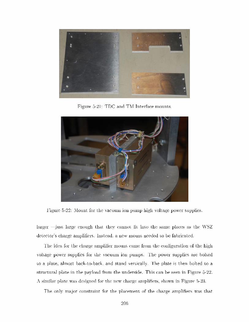
Figure 5-21: TDC and TM Interface mounts.
Figure 5-22: Mount for the vacuum ion pump high voltage power supplies.
larger just large enough that they cannot t into the same places as the WSZ
detector's charge ampliers. Instead, a new mount needed to be fabricated.
The idea for the charge amplier mount came from the conguration of the high
voltage power supplies for the vacuum ion pumps. The power supplies are bolted
to a plate, almost back-to-back, and stand vertically. The plate is then bolted to a
structural plate in the payload from the underside. This can be seen in Figure 5-22.
A similar plate was designed for the new charge ampliers, shown in Figure 5-23.
The only major constraint for the placement of the charge ampliers was that
206

Figure 5-23: XDL Charge Amplier mounting plate.
the cables connecting the detector to the charge ampliers needed to be less than
12 inches. This is because there is tremendous line loss due to the very low-voltage
signals coming from the detector. There is enough space between the longiron and
the spectrograph box on one side of the upper structural plate in the Spectrometer
Box section of the payload for this plate to be attached such that the cables to the
detectors would be short enough to prevent loss of signal from. Figure 5-24 shows
the charge amplier mounting plate.
5.3.6 Secondary Mirror Adjustment Locks
The servomotors mounted to the back of the secondary mirror of the telescope were
very precise in changing the position of the mirror so that the target would stay
centered in the eld of view even while the payload rotated in space away from the
target. However, because pointing accuracy of the ACS is good enough to point at the
target for VeSpR's pointing accuracy requirement, and because one of the servomotors
is broken anyway, this complex mechanism and its associated control electronics could
be removed from the payload, decreasing the overall mass, complexity, and number
of failure modes.
It was still desired to use the same push pins and backing plate to keep the
207

Figure 5-24: XDL Charge Amplier mounting plate
alignment of the secondary mirror during ight. For that reason, the plate, pins, and
the gears that the pins are connected to were kept while a new locking system was
built around it. Figure 5-25 shows a model of the remaining parts of the secondary
mirror mount.
The payload team had several brainstorming sessions about the best ways to lock
these mechanisms in place. A lot of time was spent researching dierent high thread-
count micrometer drives for ne optical adjustment. In the end, none could be found
that would reuse more parts and be guaranteed to survive launch loads, so it was
decided that this part should keep the same threaded inserts as well.
One of the payload team members came up with a concept to place a Teon-
backed piece of aluminum over the top of the gears and screw it down to hold the
gear in place. The Principal Investigator also required a secondary locking mechanism
in case the primary, over-the-top mechanism failed, and proposed a concept for a lock
that would put pressure on the threads directly. These two concepts were turned into
a complete design that adequately locks the mirror alignment rods in place once the
mirror is properly aligned. The design required the fabrication of a total of ten new
parts, six Teon pieces and four aluminum pieces, and only countersinking of three
208

Figure 5-25: Remaining pieces of the secondary mirror mount that were reused andlocked in place for ight.
holes on the mounting plate.
The secondary locking mechanisms consist of custom-made C-clamp-like aluminum
pieces holding another C-clamp-like ring of Teon inside. The aluminum clamps,
shown in Figure 5-26, are mirrored from each other because they are mounted above
the threaded rod insert locks, which are mirror images of each other. The Teon rings
inside the new clamps were designed to be small so that even when the aluminum
clamp is loose, there is still resistance to rotation of the gear.
One concern that arose during the brainstorming sessions was that because of
this lock, the alignment rods would not be able to go down far enough to push the
secondary mirror to the correct location. The range of motion of height of the gear
is only decreased by the thickness of the Teon ring (1/16) plus the thickness of
the top layer of the aluminum clamp (1/32). This is not a problem because in the
event that the rods do not go far enough down, more spacers can be added between
the alignment rods and the pieces that slide on top of them and directly touch the
secondary mirror.
Great care was taken to ensure that the primary mirror locking mechanisms were
209

Figure 5-26: Secondary locking clamps.
sized to the greatest precision possible. If it had been possible to put the locking
mechanisms in place without sharing a common support, then both sides of the lock
could have been the same angle relative to the base plate; however, since these parts
would overlap on one side and the gears need to be at roughly the same height,
dierent angles were needed. If one side of the lock touched the gear and the other
did not, vibrations could knock the gear (and the entire telescope) out of alignment.
Another major design constraint was the small cross-sectional area that was avail-
able to place these mechanisms. No part of the mechanism could hang over the edge
of the mounting plate because it would block light entering the telescope. Small-area
nuts were chosen over regular sized nuts to hold the support screws to the mounting
plate and to lock the angled pieces over the gears since there was not enough room
on the high-angled side for a larger nut. After ve design iterations, a design solution
for the primary locking mechanism was achieved, shown in Figure 5-27.
The Teon pieces mounted to the inside faces of the aluminum piece both come in
contact with the gear at the same time. Two #4-40 screws hold the Teon pieces in
place. On the left side, the gear touches between the two screws; on the right side, it
touches beneath the bottom screw. Figure 5-28 shows a side view the primary locking
mechanisms in place over the gears. There is enough space between the mechanisms
on the shared support screw that the gears can have up to a × dierence in height
210

Figure 5-27: Side view of primary mirror locking mechanism with Teon inserts.
and still not interfere with each other.
Figure 5-29 shows an isometric view of the secondary mirror locking mechanisms.
The centers of the gears are gripped by the Teon on the sides of the primary locking
mechanisms, and the secondary locking mechanisms grip the threads from above the
threaded insert lock that is mounted to the back plate.
All new parts were fabricated by the BU Scientic Instruments Facility, and when
assembled for the rst time, the only problem was that one of the #4-40 holes on a
primary locking mechanism was not threaded all the way through. After re-tapping
the hole, the locking mechanisms performed exactly to specications. Figure 5-30
shows photos of the nal product.
5.3.7 Semicircular Plate Modications
While the semicircular plate did not need to be moved closer to the interface plate
because of the FDR and RS-422 frames, other modications had to be made because
of its proximity to the interface plate and the new arrangement of cables required
by Wallops. Particularly, the primary low voltage power supply box needed to be
clocked nearly 120 degrees (when viewed from above) so that it was primarily located
211
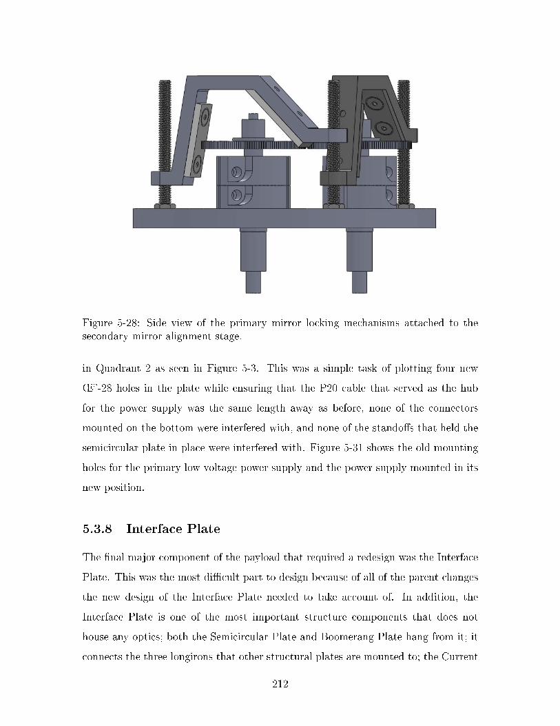
Figure 5-28: Side view of the primary mirror locking mechanisms attached to thesecondary mirror alignment stage.
in Quadrant 2 as seen in Figure 5-3. This was a simple task of plotting four new
×-28 holes in the plate while ensuring that the P20 cable that served as the hub
for the power supply was the same length away as before, none of the connectors
mounted on the bottom were interfered with, and none of the standos that held the
semicircular plate in place were interfered with. Figure 5-31 shows the old mounting
holes for the primary low voltage power supply and the power supply mounted in its
new position.
5.3.8 Interface Plate
The nal major component of the payload that required a redesign was the Interface
Plate. This was the most dicult part to design because of all of the parent changes
the new design of the Interface Plate needed to take account of. In addition, the
Interface Plate is one of the most important structure components that does not
house any optics; both the Semicircular Plate and Boomerang Plate hang from it; it
connects the three longirons that other structural plates are mounted to; the Current
212

Figure 5-29: Isometric view of the mirror locking mechanisms on the secondary mirrormount.
213

Figure 5-30: Views of the nished secondary mirror locking mechanisms.
214

Figure 5-31: Primary low voltage power supply mounted in its new location. Notethe location of the previous mounting holes where the power supply was mountedinitially.
Monitor box and Altitude Switch are mounted to its bottom face; and every cable
that runs from the experiment section to the ACS section runs through it. Ensuring
that a new Interface Plate could be made without a cascade of other changes proved
to be dicult, but after eight complete design iterations, a nal design was nished.
Early iterations of the Interface Plate were designed with poor measurements of
the locations of the holes that could not be moved. Machinists at the BU Scientic
Instruments Facility made precision measurements of the locations of the holes so
measurement errors would not be present in future design iterations. The holes that
could not change were the ones where the longiron supports and Semicircular and
Boomerang Plates attached. These holes and their associated obstruction patterns
are shown in Figure 5-32. The Semicircular and Boomerang Plates were held in place
by ÷ diameter standos, and the longirons are 2.5 x 11/16 in rectangles. Note
that all drawings in this section are aligned such that the top of the plate is at the
launch rail location, and these are views looking aft toward the experiment and rocket
boosters.
Next, the locations that are o-limits for connectors due to obstructions on the
Wallops side were drawn in place. Figure 5-3 shows some of these obstructions,
but Figure 5-33 shows them as viewed looking aft. The top, left, and right side
215

Figure 5-32: Interface Plate with required holes for the Semicircular and BoomerangPlates and tripod longiron and the area obstructed by the mounting structure beneaththe Interface Plate.
obstructions were known before design work began, but the center section was not
designated as o-limits until design iteration four.
The only major component of the payload that comes close to the Interface Plate
and could interfere with connector placement is the primary low voltage power supply.
Originally, it occupied most of Quadrant III (Figure 5-3) when looking at the Interface
Plate from this direction, but it was successfully moved so that it primarily occupies
Quadrant II with only minor obstructions in Quadrant III. The Altitude Switch and
the Current Monitor also cause some additional obstructions in the areas that are still
free for connectors, but those can be moved and mounted wherever it is convenient.
Figure 5-34 shows the area obstructed by the primary low voltage power supply in
addition to the Wallops obstructions.
Initially, there was a fear that the harness for the Analog Signals Connector (J983),
which was located in an area on the old Interface Plate that is now obstructed,
would not have enough slack to move to an unobstructed location. Soon after, the
216

Figure 5-33: Interface Plate with connector obstructions due to Wallops ACS added.
Figure 5-34: Interface Plate with connector obstructions due to primary low voltagepower supply added.
217

experiment team realized that the reason the cable had so little slack was that it was
tied down in several locations and tied to several other harnesses. After cutting these
free, there was enough slack to place the connector nearly anywhere on the plate. If
there had not been enough slack, this connector would have had to be rewired; since
this is the largest external connector in the payload, it would not have been easy.
The experiment team also wanted to take advantage of space that had been cut in
the plate that separated the Spectrometer Section from the Spectrometer Extension
Section. These cuts were made to hold harnesses in place, and now that some were
being removed, new ones could be put in their places. The connectors streaming
detector data through the telemetry (J981 and P982) are both planned to be brought
up through these cuts, which are positioned on both sides of the longiron.
It was also important to try to avoid harnesses that stretch all the way across one
section of the payload without attaching to an intermediate point. The vibrations
and accelerations the payload experiences during launch can shake harnesses with
too much slack strongly enough to rip connectors out of their sockets or wires out of
the connectors. This is why the Star Tracker (J733) and Xybion camera power input
(P984) and data output (J986) are squeezed into areas that are close to obstructions.
All three of these cables move up the payload along the longiron support located
closest to launch rail, so they have been positioned as close to the launch rail as
possible.
The remaining harnesses connecting to the Interface Plate all originate from center
origins in the payload and can be easier moved or fabricated to t in nearly any
location in the unobstructed area. Figure 5-35 shows the nal design of the Interface
Plate with all the connectors and holes for the Altitude Switch and Current Monitor
Box labeled. Figure 5-36 shows the nished Interface Plate mounted on the payload.
5.3.9 Mechanical Design Change Review
Despite careful planning and mapping out design details as well as possible in advance,
there are design changes that are perhaps more costly or not as optimal as they could
have been. Sometimes the desire to reuse parts actually added to the total cost, as
218

Figure 5-35: Final Design of the Interface Plate.
219

Figure 5-36: Finished Interface Plate.
in the case of the secondary mirror locks, due to the amount of custom machining
necessary for the concept to work. In other cases, the total costs were not compared
adequately with their alternatives, such as in the case of choosing to refurbish the
detectors versus purchasing new ones, where the cascade of design changes due to
that choice may have cost more in the end than simply paying for refurbishment.
In all cases, optimality in the design was not considered nearly as much as it is
when designing other spacecraft systems. There was no strict requirement to minimize
the total mass of the new components, only the desire to have the mass lower than it
was in previous ights. Practices were used to avoid low-frequency resonance modes
like osetting screw locations, but these were not backed up with solid calculations.
Engineers at the Kavli Institute assured the payload team that the thermal capacity
of the aluminum frames was enough to prevent the electronics from overheating in
vacuum; this is known from experience to be the case, but no formal heat transfer
analysis was conducted.
One of the key problems in designing components to see how they aect the entire
system is a lack of a complete solid model of the payload. Some of the pieces of this
payload date all the way back to 1967; other parts are from the early 1990's at the
latest. In all cases, there is no way to predict the vibration modes, stresses, strains,
220

and factors of safety within the structure before taking the payload to Wallops for
systems integration. Building a solid model was considered too time-consuming to
the Principal Investigator for this ight, but for future ights or rebuilds it may be
worthwhile to have a solid model to do a complete structural and thermal analysis.
Any ight engineer working on this payload in the future can use such a solid model
and verify its accuracy against test data from the rst VeSpR ight's integration
testing.
5.4 Designing Payload Ground Support Equipment
Since the output of the TM Interface and the communication software Wallops is now
using are both completely dierent from the ones used on the previous JASpR ight,
the payload GSE needed to be updated to work with the new systems. In addition,
the source les of the software used to read the data cannot be found. Rather than
updating the GSE software to work with the new hardware, the science team decided
to develop a whole new system.
The GSE computers, as described in Section 4.2.6, were considered obsolete even
during the last JASpR ight. In addition, today's computers are so much more
powerful that there is absolutely no need to have two computers; one computer should
be able to receive, process, and display all of the incoming data from the rocket.
Furthermore, there was a desire to make the computer system more portable, not only
during integration testing at WFF and WSMR but also during calibration testing at
BU and verication testing at MIT. Carting around two large computers, the bit
encoder, the spaghetti box, and a power supply and keeping track of the cables
and their proper connections was a hassle that the science payload team wanted to
eliminate. A laptop with input devices is all that is needed.
The new GSE computer equipment also does not need nor is the payload team
able to acquire a PCM identical to the one that will be used in ight to replicate com-
munications with the TM Interface. Rather than having using the PCM to convert
the parallel data into a radio signal and having the Bit Sync convert the radio signal
221

back into parallel data, the parallel data can be read directly from the TM Interface.
Data input requirements for the GSE remained virtually unchanged. While it is
desired to view data from both detectors at the same time, both are not required
to be monitored and displayed at the simultaneously. During component calibration
testing, only one detector is used at a time, and when the payload is fully assembled,
the input cables can be easily switched between the spectrograph and the imager
detectors. Only one 32-bit parallel data stream needs to be monitored at a time. The
analog monitor signals remain unchanged.
Another sounding rocket team at BU uses an AccesIO Products Inc. 16-bit USB
Digital Input Module to read 16-bit data from one of their detectors. Their experience
and willingness to provide an initial program to read data and help troubleshoot if
the VeSpR team decided to use similar products was a major factor in deciding what
input modules would be used in the GSE. The downside to this choice was that
AccesIO only has 16-bit digital input modules that can read input data. The VeSpR
detectors have a 32-bit output. If the VeSpR team had been able to acquire a 32-bit
module for a reasonable price, both streams of data from the detectors could have
been displayed simultaneously. This is an improvement that can easily be made in
the future if such a 32-bit module became available.
Figure 5-37 shows the conguration of the new GSE data input system. The
system consists of one laptop computer, three data input modules, a custom timing
circuit, and associated wiring, terminal boards, and connectors. The whole system
ts in a 15 x 21 x 6 in plastic storage bin that can be easily carried anywhere and
does not require external power as long as the laptop batteries are charged. What
once required continuous A/C power, weighed over 100 lbs, and could not be moved
without careful planning has been replaced with this < 25 lbs system that can be
taken nearly anywhere.
The computer is a Lenovo Thinkpad with three USB ports that runs Ubuntu, a
Linux-based operating system. Linux was chosen over other operating systems for
several reasons. Astronomers typically use IDL (Interactive Display Language) to
display, reduce, and analyze data, typically on Macs but it is also easily compatible
222

Figure 5-37: New GSE computer setup
with Linux (all work in Chapter 6 was done in IDL on a Mac). It is dicult to run
IDL on a Windows operating system and it is not user-friendly. While the science
team has more experience with Macs, the computer support sta members at BU are
experts with Linux. In addition, the AccesIO digital input modules are compatible
with Windows platforms but can be easily patched to operate with Linux platforms.
Linux was therefore the logical choice because of these reasons.
The laptop connects to three AccesIO input modules; two USB-DIO-16A input
modules capable of reading 16-bit digital input/output, and a USB-AI12-64ME analog
input module capable of reading 64 analog inputs with 12-bit resolution (more on the
analog signals later in this section). These cards are far more capable than they
are required to be to sample at the same rate as the telemetry, but most computer
components nowadays are. The digital input modules can read data at speeds of up
to 40 MHz even though the updated telemetry requirement is 25 kHz, and the analog
module can sample the analog monitors at speeds of up to 100 kHz even though the
telemetry samples the analog signals at only 10 Hz.
Since the digital input modules have only 16 channels and the detector output
from the TM Interface uses 32-bits, half of the outputs go to one module and half
223

go to the other. Another piece of hardware was needed to properly sync the two
inputs. A small timing circuit ensures that the two cards are reading data at the
correct frequency and phase. This sets up the cards so that one module is a master
and the other is the slave, which ensures that the computer is reading the two 8-bit
words from each of the two digital input modules in the correct order that they are
sent from the TM Interface. If 32-bit input cards are available for a low price in the
future, this timing circuit will not be necessary.
Both digital input modules connect via USB to the GSE laptop. Data from the
detectors coming through the modules is displayed on the laptop in real time using
an IDL program. The other BU sounding rocket science team also provided a version
of this program that was modied to correctly display the data from the two 16-bit
modules. Just like the original display program on the DOS computer, it displays the
total photon counts, the current count rate in counts per second, the total number of
rejected counts, and the total number of bad counts.
The analog input module reads the analog monitors. Although the payload only
has 32 monitors, a 64-input module was used in case a future ight ever needed more
analog signals to be read. A custom graphical user interface was developed that
displays the voltages on the monitors in real time. These monitors are recorded in
ight as data that is given to the science team once the mission is completed. For
ground testing, these monitors only serve as points that need to be checked against
test values to monitor payload health, so it does not matter that they are not sampled
at the same rate as they will be sampled in ight.
5.5 Data Expectation Modeling
Even though the capabilities of VeSpR have been improved since the JASpR missions,
a model of what the expected data output of the spectrograph detector would produce
is needed to verify that the system is capable of meeting the system requirements to
achieve the scientic objectives. Building models that match experimental data give
condence in the ability of the instruments to meet these objectives in ight.
224

Table 5.2: Telescope sizing properties used to calculate the total light collecting area.Telescope Size Properties Value Units
Primary Mirror Diameter 35.0 cmPrimary Mirror Area 962.1 cm2
Secondary Diameter 12.0 cmSecondary Area 113.1 cm2
Tripod Support Thickness (Each) 6 cmTripod Support Area (Total) 207 cm2
Total Telescope Collecting Area 642.0 cm2
First, a model of the telescope and spectrograph optics and the spectrograph
detector were created to predict the overall throughput of the system. Next, the
observation targets were modeled according to their expected position, velocity, and
brightness. These two models were combined to calculate the expected count rate,
total counts, and the uncertainty in the data taken during ight, and a model spec-
trum was produced that should match what is seen in ight. The IDL code and Excel
spreadsheets for all of these steps are available in the attached Appendix DVD.
5.5.1 Modeling Telescope and Spectrograph Optics
Models of the telescope and spectrograph optics were developed previously for the
JASpR ights in a ray-tracing program called BEAM4. Since the actual optics have
not changed, this model was reused to argue that the telescope and spectrograph
could achieve resolution of 1-2 arcsec each and a combined resolution of 2-3 arcsec.
This had been shown in early VeSpR calibrations as well, and this information will
be considered later in the modeling process.
The rst step of the VeSpR modeling process was to nd the total light collecting
area of the telescope. The primary mirror has a diameter of 35cm, but since the
telescope is a Cassegrain design, the secondary mirror and secondary support beams
obstruct the view of the primary and block some of the incoming light. Table 5.2
shows information on how the total light collecting area was calculated.
Figure 5-38 shows the BEAM4 model of the telescope and spectrograph box. Light
reects o the primary and secondary mirrors and passes through the objective prism.
225

Figure 5-38: BEAM4 model of the path light takes from the telescope to the spectro-graph detector.
Light then passes through the spectrograph spit and enters the spectrograph box.
Light reects o the parabolic mirror, then the echelle grating, then the parabolic
mirror again before going through the magnesium uoride window and into the de-
tector. In total, light entering the telescope interacts with 7 dierent optics before
reaching the multi-channel plates in the detector.
All of the major optics except for the echelle grating were sent to NASA Goddard
Space Flight Center to be polished and recoated to achieve maximum UV reectivity.
The aluminum mirrors over-coated with magnesium uoride can achieve reective
eciencies of over 80%, which is better than what was measured during initial cali-
bration testing for these optics (see Section 4.5). For a nominal case, 75% eciency
is assumed. Table 5.3 shows estimated eciencies for all of the components of the
telescope and spectrograph box at Lyman-alpha wavelengths.
A 0.278% total eciency for the whole system means that the spectrograph and
telescope have an eective collecting area of 1.79 cm2.
The existing BEAM4 model also showed that the plate scale at the focal plane
was 26 arcsec/mm. The new XDL MCP detectors have a grid resolution of 25 µm,
226

Table 5.3: Estimated eciencies at Lyman-alpha wavelengths of all of the optics tothe spectrograph detector.
Throughput/Reective Eciency %
Telescope Optics PropertiesPrimary Mirror Eciency 75.0Secondary Mirror Eciency 75.0Objective Prism Eciency 40.0Total Telescope Eciency 22.5Spectrograph Optics PropertiesParabolic Mirror Eciency 75.0Echelle Grating Eciency 20.0Parabolic Mirror Eciency 75.0Total Spectrograph Eciency 11.3Detector Subsystem PropertiesWindow Eciency 50.0Detector Quantum Eciency 22.0Total Detector Subsystem Eciency 11.0Total VeSpR Optical Eciency 0.278Eective Telescope Collecting Area 1.79 cm2
Table 5.4: Additional instrument properties and spectrograph detector resolution.Property Value Units
Plate Scale 26.0 arcsec/mmDetector Resolution 25.0 µm/pixelImage Sizing 0.65 arcsec/pixel
which is half the size of the old WSZ detector grid resolution of 50 µm. Table 5.4
shows these properties and the resultant angular pixel size.
The nal step in building a model of the telescope is to nd a line-spread function
(LSF) of the telescope and spectrograph. At the time of this writing, a true LSF
for the payload has not been measured, but Figure 5-39 shows the LSP found dur-
ing JASpR testing measured at Lyman-alpha generated in IDL. The full-width half
maximum (FWHM) at Lyman-alpha is 0.055 Å. This LSF was used to model the
measured spectrum, described in the next section.
227

Figure 5-39: Model point spread function of the VeSpR telescope, spectrograph, anddetector.
228

Table 5.5: Venus ephemeris data for April 4th, 2012, the date of Venus' maximumvelocity relative to Earth, and telescope scaling properties on that day.
Property Value Units
Date of Launch April 4th, 2012 Day of Year 95 Right Ascension 3.80 hoursDeclination 23.77 degAngular Diameter 25.7 arcsecDistance from Earth 9.714x10⁷ kmRelative LOS Velocity 13.445 km/sBlue Shift 0.055 ÅSun-Earth-Venus Angle 45.8 degPlate Scale 26.0 arcsec/mmDetector Resolution 25.0 µm/pixelImage Sizing 0.65 arcsec/pixelAngular Sizing 471.0 km/arcsecPixel Sizing 306.1 km/pixel
5.5.2 Modeling Targets and Background
During ight, VeSpR will be observing Venus through the top layers of Earth's atmo-
sphere and through interplanetary space. The launch window has been determined
by the Principal Investigator to be when Venus is moving towards Earth so the hy-
drogen and deuterium spectra of Venus are blue-shifted away from Earth's geocoronal
emission.
The NASA Jet Propulsion Laboratory's HORIZONS On-Line Solar System Data
and Ephemeris Computation Service was used to generate a ephemeris displaying
daily positioning information for Venus during the year 2012. This ephemeris data
showed that near April 4th, 2012, Venus will have a maximum line-of-sight (LOS)
velocity relative to Earth, 13.445 km/s, during this synodic period. If this date were
chosen as the launch date, it would create the maximum blue-shift. Coincidentally,
the blue-shift at maximum LOS velocity is 0.055 Å, which is very close to the FWHM
of the LSF. Table 5.5 shows a sample of the data from this ephemeris on April 4th.
The full table is available in the attached Appendix DVD.
Another program developed for use with JASpR data was used to calculate the
LOS velocity of the interplanetary medium (IPM), which is composed of neutral
229

Table 5.6: Estimated brightnesses of Venus and elements of the sky background.Emission Value Units
Venus Hydrogen 9000 RayleighsVenus Deuterium 500 RayleighsEarth Hydrogen 5000 RayleighsEarth Deuterium 50 RayleighsInterplanetary Medium 500 Rayleighs
hydrogen in space that also reects and scatters solar Lyman-alpha light. An observer
looking in the direction of Venus on April 4th, 2010 when it is at the declination
shown in Table 5.5 will have an LOS velocity relative to the IPM of 22.18 km/s,
corresponding to a 0.090 Angstrom red-shift of the IPM Lyman-alpha emission. Even
though the IPM emission is faint, observing Venus when it is blue-shifted while the
IPM is red-shifted reduces the overlap between the two emissions and increases the
signal-to-noise ratio.
The brightness of Earth's geocoronal emission and the IPM are well known from
other Lyman-alpha studies. The brightness of Venus' hydrogen is also known, and
the deuterium emission has been estimated based on existing D/H ratios (see Section
3.2). Table 5.6 shows the initial estimated brightnesses of the spectra that will be
visible on the detector.
The spectrograph aperture is 5 arcsec wide, so the solid angle of the targets can
be calculated. With the solid angles, eective light collecting area, and total time
observing the target (275 seconds in the nominal mission prole), the brightness of the
targets in units of Rayleighs (106 photons/cm-s into 4π steradians) can be converted
into a photon count rate. Table 5.7 shows the solid angles of Venus, the minimum
resolvable area, and the entire sky when viewed through the spectrograph aperture.
5.5.3 Model Results
Table 5.8 shows the count rates in photons per second measured by VeSpR for Venus
deuterium and hydrogen measured as a bulk of the planet (25.7 arcsec) and Earth
hydrogen and deuterium and the IPM for the entire sky background. The table also
230

Table 5.7: Model target and sky solid angles.Property Value Units
Venus Diameter 25.7 arcsecTotal Venus Area 128.5 arcsec2
Minimum Resolution 2 arcsecMinimum Resolvable Area 10 arcsec2
Aperture Slit Length 300 arcsecTotal Sky Area 1500 arcsec2
shows the expected total counts received by each source throughout the ight and the
Poisson uncertainty as a function of counts and a percentage of the measurement.
Notice that the expected total count rate is much less than the maximum rate that
the TM Interface can send data through the telemetry (25,000 counts per second) and
even less than the rate at which dead time eects cause error in the detector's output
(100,000 counts per second). Also note that the Venus deuterium count rate is based
o of the bulk planet rather than a function of altitude, the count rate calculation
was applied to the lowest spatial resolution of the spectrograph. Table 5.9 shows the
results for the expected spatial resolution element of 2 arcsec, which corresponds to
a distance of 940 km.
An IDL program written previously by the Principal Investigator already exists to
model spectral data from HST. This program was heavily modied to model spectral
data for VeSpR. A model spectrum was generated by modeling the expected emissions
from Venus and the sky background as Voigt proles convolved with the VeSpR
telescope and spectrograph LSF. A Voigt temperature of 300 K was assumed for
Venus' upper atmosphere. Figure 5-40 shows the model hydrogen and deuterium
spectra of Venus generated in IDL.
A Voigt temperature of 1000 K was assumed for Earth's upper atmosphere for
Earth's geocoronal emission, and 30,000 K was assumed for the IPM because it is
so broad (see Section 2.5 for more on Voigt proles). Both of these were compared
to geocoronal sky backgrounds taken by Hubble's STIS (see Figure 6-16) to ensure
accuracy and then convolved with the VeSpR PSF. Figure 5-41 shows the model
spectrum of the geocoronal background and the IPM.
231

Table 5.8: Calculated results for counts, count rates, and uncertainty in the measure-ments for the entire disc of the planet.
Measurement Value Units
Venus Deuterium Count Rate 2.15 counts/sVenus Deuterium Total Counts 591 countsVenus Deuterium Uncertainty (absolute) 24 countsVenus Deuterium Uncertainty (relative) 4.11 %Venus Hydrogen Count Rate 38.66 counts/sVenus HydrogenTotal Counts 10632 countsVenus Hydrogen Uncertainty (absolute) 103 countsVenus Hydrogen Uncertainty (relative) 0.97 %Earth Hydrogen Count Rate 251 counts/sEarth Hydrogen Total Counts 68949 countsEarth Hydrogen Uncertainty (absolute) 263 countsEarth Hydrogen Uncertainty (relative) 0.38 %Earth Deuterium Count Rate 2.51 counts/sEarth Deuterium Total Counts 690 countsEarth Deuterium Uncertainty (absolute) 26 countsEarth Deuterium Uncertainty (relative) 3.81 %IPM Count Rate 25.07 counts/sIPM Total Counts 6895 countsIPM Uncertainty 83 countsIPM Uncertainty 1.20 %Total Count Rate 319.11 counts/sTotal Counts 87755 counts
Table 5.9: Calculated results for Venus deuterium counts at a resolution of 2 arcsec.Result Value Units
Venus Deuterium Count Rate 0.17 counts/sVenus Deuterium Total Counts 46 countsVenus Deuterium Uncertainty (absolute) 7 countsVenus Deuterium Uncertainty (relative) 14.75 %
232

Figure 5-40: Model Venus hydrogen and deuterium spectral proles convolved withthe VeSpR telescope and spectrograph PSF. Venus hydrogen is shown in yellow,deuterium is shown in green.
Figure 5-41: Model sky spectral proles of Earth hydrogen and deuterium and theinterplanetary medium (IPM) convolved with VeSpR telescope and spectrograph PSF.Earth hydrogen is shown in blue, the IPM is shown in red, and Earth deuterium isbarely visible at 1215.34 Å.
233

Figure 5-42: All Venus and sky spectral proles convolved with VeSpR telescope andspectrograph PSF.
Both the Venus spectra and the sky background spectra are shown on the same
spectrum in Figure 5-42. The nal spectrum is shown in Figure 5-43. Notice the two
peaks from Venus and Earth hydrogen Lyman-alpha are resolvable.
5.5.4 Sensitivity Analysis and Model Limitations
The modeling results presented in the previous subsection are based on many as-
sumptions for values that may not be correct when VeSpR is launched. An analysis
of how the results can change with dierent parameters will determine how robust
the system is and if it can achieve the science objective as the actual performance
changes from the nominal performance.
The launch date is of course subject to change. VeSpR was originally scheduled to
y in July 2010 but was delayed because WFF was backed up with other customers.
Scheduling conicts may place VeSpR's launch earlier or later than the ideal date,
payload integration may take longer than planned, and weather can cause a scrubbed
launch. It is important to know how the conditions will change with the launch date.
234

Figure 5-43: The expected spectrum that VeSpR will observe the estimated bright-nesses of Venus and elements of the sky background (see Table 5.6).
Figure 5-44 shows the relative velocity between Venus and Earth and how it
changes throughout the year 2012. There is a long period of time where the relative
approaching velocity of Venus exceed 10 km/s in the beginning of 2010 before it
quickly moves between the Earth and the Sun.
The relative velocity is important to resolve the deuterium line prole spectrally;
however, because the distance to Venus is decreasing rapidly while Venus emissions are
highly blue-shifted, the angular size of Venus is increasing. This increase in angular
size corresponds to an increase in spatial resolution and a higher count rate. Delaying
launch past the date of maximum relative velocity may increase the performance of
the experiment. Figure 5-45 shows Venus' distance relative to Earth as it changes
throughout 2012, and Figure 5-46 shows Venus' angular size as viewed from Earth
during that same period.
On May 13th, 2012, the relative velocity of Venus slows below 10 km/s, but
it is almost 55% closer and has an angular diameter of 45.4 arcsec. This means
the telescope can achieve a spatial resolution of 520 km with 2 arcsec image quality
compared to 940 km on April 4th. Figure 5-47 shows the nal spectra given ephemeris
235

Figure 5-44: Venus' line-of-sight (LOS) velocity relative to Earth as a function of theday of the year in 2012.
Figure 5-45: Venus' distance relative to Earth as a function of the day of the year in2012.
236

Figure 5-46: Venus' angular diameter as seen from Earth as a function of the day ofthe year in 2012.
data for May 13th. Notice how even though the peaks of the Venus and Earth
hydrogen Lyman-alpha proles are not resolvable like they are in Figure 5-43 but
that the deuterium peak is still resolvable.
This model does not take into account how the sky brightness changes as Venus
gets closer to the Sun. On May 13th, the angle between Venus and the sun is only 31.5
degrees from the Sun, and the angle of the ecliptic may not be near perpendicular with
the horizon, so the sky brightness and spectral width may increase by high enough
factors that it would be impossible to spectrally resolve the deuterium emission of
Venus.
In addition, as Venus gets closer to the Sun, a smaller fraction of the planet will
be illuminated. The disk of the planet will start to become crescent-shaped and the
solid angle that is illuminated will decrease, which would rapidly lower the overall
count rate especially when the width of the illuminated crescent is less than 5 arcsec.
Since this parameter is sensitive to pointing accuracy and is
Great care is taken in payload maintenance, laboratory testing, shipping, and
launch preparations to ensure that the optics are kept as clean as possible. Since
ultraviolet light interacts with so many optics, degradation of the optics has a multi-
237

Figure 5-47: The expected spectrum that VeSpR will observe on May 13th.
plicative lowering of the overall eciency. If the eciency of one optic is cut in half,
the entire system is half as ecient; if the eciency of two optics are cut in half, the
entire system is only one quarter as ecient.
If every aluminum mirror degrades from 75% to 70% eciency, then the total e-
ciency goes down from 0.278% to 0.211%. This would decrease the eective telescope
area down from 1.79 cm2 to 1.35 cm2. The error in the deuterium measurement of the
bulk planet would rise from 4.11% to 4.72%, and the error in the measurement at the
best resolution would increase from 14.75% to 16.93%. If the entire payload optical
eciency falls down to 0.5%, the bulk and best resolution deuterium measurement
errors would be 6.87% and 24.61% respectively.
Although the brightness of Venus' deuterium Lyman-alpha emission estimated
based on data from past experiments, how it varies is unknown; after all, the goal of
VeSpR is to measure D/H at the top of the atmosphere. If the brightness in areas
of the atmosphere is actually only 100 Rayleighs, the bulk and best resolution errors
would be 10.56% and 37.86%, respectively. An undetectable deuterium emission
would also be a major nding assuming the total eciency of the system is high
238

enough to measure brightness that low.
The brightness of Earth's deuterium line is also dependent on the launch window
and time. The estimate of 50 Rayleighs brightness may be too low, and if it rises
it would overlap with the Venus deuterium emission. Even though the relative error
goes down as brightness goes up, the absolute error goes up as the square root of the
brightness, which adds uncertainty in the data when the sky background is subtracted
(see Section 6.3.2 for more on sky subtraction and error propagation). The possible
variations in Earth's deuterium emission are an argument against having a launch
date closer to May 13th than April 4th since the ability to resolve the two becomes
harder at lower blue-shifts.
In the near future, this model can be modied to be more accurate in many ways.
Full payload calibration will result in a total quantum eciency measurement of the
entire payload and an accurate PSF, both of which can be easily implemented to give
more realistic results.
5.6 Final Payload Testing
Even though the VeSpR ight was delayed from July 2010 to February 2012, there
are still many tasks ahead for the payload team. Although all the components of
the new design have been completed, there is still signicant testing required before
VeSpR is ready for ight. Delays in Wallops readiness caused slips in the BU team's
schedule. Resources at BU must also be shared with other rocket projects; when the
VeSpR ight was delayed, testing in the VUCL had to stop so another rocket team
could use the vacuum chamber for their testing. That team is still using the labora-
tory, so calibration of the recoated optics has not yet occurred. This section details
nal testing on components that has already been done and outlines the remaining
construction and testing required over the next year.
239

Figure 5-48: Flow of digital data in the initial TM Interface test at WFF in March2010.
5.6.1 Testing the TM Interface, FDR, and GSE
The TM Interface was the rst piece of the payload that was formally tested at
NASA's Wallops Flight Facility (WFF). Integration testing was originally scheduled
for March 2010 because the payload was originally scheduled for launch in July of that
year. However, due to delays in other launches that WFF handles and the shifting
duties in personnel on various projects, components for the VeSpR payload were not
ready for testing. The only components of the payload that were tested during the
scheduled integration were the skin sections and the TM Interface.
At this time, the new MCP detectors had not been removed from their shipping
crates, so rather than having actual MCP data input to the TM Interface, simulated
data was created using an AccesIO USB-DIO-32 module. This module was originally
purchased because its product specications made it appear to be capable with 32
bits of data what the USB-DIO-16A is capable of doing with 16 bits (Section 5.4).
Even though USB-DIO-32 module could not record digital data coming from the TM
Interface, it was very useful during testing to send digital data to any component it
was connected to.
A laptop was connected to the USB-DIO-32 module. The module was then con-
nected to the TM Interface, which was then connected to a module that is used to
simulate the WFF PCM stack for ground testing. This data chain is shown in Figure
5-48. This simulated PCM module's output was connected to the USB-DIO-16A and
GSE laptop. Simulated 32-bit detector data was sent through the USB-DIO-32 to the
TM Interface. The TM Interface output parallel data that was read by the Wallops
GSE module. The Wallops GSE module had a graphical user interface (GUI) that
displayed the 32-bit data as four hexadecimal letters, and these hexadecimal letters
matched what was being input.
240

In the rst test, data from the Wallops GSE module was being ipped as it came
through the USB-DIO-16A into the GSE laptop; the last two letters of the data were
not in the right order. The electrical engineer notes that this particular Wallops GSE
module was faulty, and another was brought to replace it. This time, the data stream
was read in the correct order. The payload team requested that a third Wallops GSE
module be used to verify that the test was accurate, so a third module was tested
with the TM Interface. Again, data was coming through as expected.
Later testing at the MIT Kavli Institute tested the TM Interface, the FDR, and
the GSE all together. Again, simulated detector data was input to the TM Interface.
The TM Interface then output parallel data to the GSE, which simulated the WFF
PCM module, and the FDR. First, data was sent from the USB-DIO-32 through the
TM Interface and USB-DIO-16A module to the GSE laptop. It was veried that all
32 bits of parallel data were being read in the correct order.
Next, the system was powered down and the SD card was removed from the FDR.
There was one le on the FDR with a le name corresponding to the time that power
was rst supplied to the TM Interface and FDR. This le had recorded 32 bits of
data at a rate of 25 kHz with the same sequence of changes corresponding to the
same times that changes were made in the data coming from the USB-DIO-32 during
the test. The le also did not record data after the USB-DIO-32 was powered down,
indicating that the FDR was not recording ll data being sent by the TM Interface
when no data was coming from the simulated detector data stream. Although this
was not an ocial acceptance test, it did prepare the team for acceptance testing.
5.6.2 Testing the High Voltage Power Supplies
Small and aordable high voltage power supplies that are qualied for spaceight
are dicult to nd since the SPACOM Corporation dissolved. Rather than nd new
ones to supply high voltage power to the detectors, the old ones could be re-tuned
to supply the correct voltage for the new detectors. Two pins on the input 9-pin
connector are attached to a tuning resistor to determine the output voltage of the
supply. Inside the payload, the tuning resistor used to tune the voltage for the old
241

detectors is permanently encased in potting on the connector itself. It will need to
be replaced, but the exact resistance needed was unknown, so all the power supplies
were tested.
There are ve high voltage power supplies that have been used to power the
detectors or were purchased as backups. Of the ve, one was previously declared
unusable back in the JASpR time period. Only one of them came with a test report
that showed how output voltage varied with input voltage and tuning resistance, and
since the report was generated more than 15 years ago there was no guarantee this
was accurate for that power supply.
Figure 5-49 shows the setup used to test the detector high voltage power supplies.
The supply is mounted to the breadboard in the top center of the gure. The 9-
pin connector on the input side of the supply is connected to the terminal board so
that the input voltage, output monitor, and input resistance can be supplied and
monitored using multimeters. The potentiometer mounted to the bottom left of the
breadboard was used to vary the input resistance from 6 kΩ down to 900 Ω, which
corresponds to -2000 V and -6000 V output for the power supply according to the
specication sheet that was available for one of the supplies. The output of the power
supply was connected to a 1/1000 voltage divider encased in silicone to prevent high
voltage arcing. The resulting output voltage is read on a multimeter and is close to
1/1000th of the actual output voltage.
Initial tests failed because there was a short in the voltage divider. The old box
was gutted, new 1 GΩ and 1 MΩ resistors were purchased, and the whole box was
rebuilt with a new Reynolds high voltage connector. Silicone potting was mixed,
vacuumed, poured into the box, and vacuumed again until no more bubbles were
rising to ensure that all air had escaped from the inside and there was no danger of
high voltage arcing when connected to a high voltage power supply. The divider was
tested with a laboratory high voltage power supply while connected to a multimeter.
This test showed the voltage divider actually divided the input voltage by 1100 V.
Figure 5-50 shows a closer view of the rebuilt voltage divider.
Next, each power supply was tested individually. The test setup was connected to a
242

Figure 5-49: Detector high voltage power supply testing setup.
Figure 5-50: The rebuilt voltage divider used to test the output from the high voltagepower supplies.
243

supply and the resistance of the potentiometer was measured before power was turned
on. The output voltage was recorded, and then power was turned o. Once power
dissipated from the system, the resistance was measured and changed. Each power
supply was tested at 11 dierent resistances to generate a function to determine the
output voltage given an input resistance. The input voltage was not varied between
+24 V and +32 V, which was a test the specication sheet also showed, but since the
change in voltage has little eect on the output and no signicant change in voltage is
expected in ight, this did not matter. In addition, the resistance function was tested
at a higher resolution, 11 samples compared to the specication sheet's 5 samples.
The testing showed that the power supply that had originally been labeled un-
usable was still working, even though it will not be used in ight without further
testing. In addition, the input resistance for the necessary output for the detectors
for every power supply was found to be within a 20 Ω range, so if a power supply fails
during testing, it can be switched out without requiring a change in the input resistor.
All of the supplies are the same model, but the variations between performances still
needed to be measured for this assumption. The full results from high voltage power
supply testing are available on the attached Appendix DVD.
5.6.3 Future Testing and Construction Plan
As stated previously, the division of resources available at BU has caused some delay
in the nal testing of the payload optics and the new MCP detectors in the VUCL.
In addition, the team has encountered problems with the collimating mirror in the
VACTEF vacuum chamber, delaying future work for full payload testing. Work is
currently underway to realign and reinstall the mirror in the chamber for full payload
testing. Without this mirror, a full payload absolute calibration cannot be made
in the VACTEF. While progress on Project VeSpR has been hampered, the science
team members have been working on additional projects (see Chapter 6), laying the
groundwork for changes in the VACTEF to be capable of testing future space ight
hardware, rewiring the harnesses that have changed to connect to the payload during
vacuum testing, and documenting the new state of the payload to save future team
244

members time so they do not have to sift through two decade's worth of notebooks
from previous payload ights.
The rst test the science team will conduct is activating the new XDL MCP
detectors. Simply activating the detectors and reading data will do the following;
conrm that the detectors were not damaged in shipping; verify that the output
cables from the detector are the proper lengths to induce the needed line delay; test
the GSE, TM Interface, and FDR with actual MCP data, allowing the components
developed by the Kavli Institute to be ocially accepted; display MCP data on the
GSE computer in real time; and obtain at eld exposures that can be compared
with the test report that Sensor Sciences provided for the detectors.
It has still not been ocially decided whether the electronics developed at the
Kavli Institute will be potted after they have been tested with the MCP detectors
or immediately before the Vibration Test during integration testing. The electronics
will not be potted before this test because if any modications are needed to the
board, they cannot be made after the board has been potted. The electronics must
be potted before the Vibration Test because they will not survive without potting.
The decision will be made once WFF informs the payload team whether or not they
will be ready for integration testing in spring 2011 (see Section 5.6.4 for more in
integration testing). Potting of the electronics and connectors can be done at BU,
MIT, or WFF.
After testing and calibrating the MCP detectors, the spectrograph box will be
aligned. First, all the components except the coated optics will be bathed in iso-
propanol and acetone, and what components are small enough to t in the ultrasonic
bath in the VUCL will be cleaned in there as well. Next, the spectrograph box will
be reassembled in the VUCL clean room and placed in the vacuum chamber. The set
screwed will be turned to the heights that were determined in previous testing to be
where the grating is aligned such that the 221st order of Lyman-alpha will be visible
on the detector. The spectrograph box will be aligned in the vacuum chamber with
a green laser before the chamber is pumped down and the alignment is checked. If
the Lyman-alpha emission line is not centered on the detector, the set screwed will
245

be measured again and turned to the correct height. Once alignment has been found,
the top plates that secure the grating will be installed and alignment will be checked
again. Finally, an absolute calibration of the detector with the spectrograph box will
be made. Now that the team has considerable practice with this tedious endeavor, it
should not take nearly as long as it did during initial payload testing (Section 4.5).
Next, the telescope secondary mirror will be aligned with the VACTEF collimating
mirror. The secondary mirror adjustment locks (Section 5.3.6) will be installed and
the pushrods will be screwed into place so that the telescope has an optical quality
of at least 2 arc sec. Once this has been achieved, the two locking mechanisms will
be tightened and the alignment will be checked again to ensure that tightening the
locks did not misalign the secondary mirror. The telescope will then be moved to
the VACTEF and absolutely calibrated with the PMT (now that the PMT has been
absolutely calibrated, the same setup that was described in Section 4.5 to obtain a
relative calibration can be used to obtain an absolute calibration).
Next, the entire payload will be reassembled for full payload testing in the VACTEF
vacuum chamber. The required screws and other supplemental hardware have already
been purchased and the majority of the payload can be reassembled at any time. First,
optical alignment of the spectrograph, imager, and Xybion camera will be checked.
The Xybion camera will be aligned at atmospheric pressure with a visible light before
the chamber is pumped down. The imager detector and Xybion camera should see
the same eld of view because they are mounted on the same structure, which has
not changed. The alignment of the spectrograph box may need to be further adjusted
with the Teon supports mounted in the plate that separates the Spectrometer Sec-
tion from the Spectrometer Extension Section. Since the VACTEF can be quickly
brought to air and pumped down again, this will not take as long as the spectrograph
alignment in the VUCL will.
Finally, an absolute calibration of the spectrograph and imager detectors will be
made. If the total system performance is not adequate to achieve the science goal (Sec-
tion 5.5), the payload will be taken apart to locate the degradation in the eciency.
Since the spectrograph box and telescope will have been absolutely calibrated before
246

the full payload test, there should not be a signicant degradation in the eciency in
any optics compared to their calibration tests. If there is, this could mean contam-
ination in the vacuum chamber. Both the VUCL and VACTEF vacuum chambers
will be checked for contamination using a mass spectrometer, and individual optics
testing will be conducted again.
Once the payload has been thoroughly tested, it will be placed back in storage in
the shipping crate that will be used to transport it to Wallops. Power will still be
supplied to the VIPs so the MCP detector housings stay at vacuum.
5.6.4 Integration Testing Plan
Integration testing will take place at WFF in spring or summer 2011, but the date
has not been ocially scheduled at this time of writing. Preliminary estimates from
VeSpR's new Mission Manager indicate that WFF will still not be ready for integra-
tion testing by March; it may be delayed until the summer of this year. The Integra-
tion Testing Plan was put forward during the Design Review and has not changed
since then. Integration Testing consists of instrumentation, power, and mechanical
tests on the payload to ensure that all components are communicating properly and
that the system is structurally capable of withstanding launch loads without failing
or losing optical alignment during launch.
5.6.4.1 Instrumentation Tests
The rst phase of the instrumentation tests is the Pre-Vibration TM Electrical Check-
out. This test will be performed based on a customized version of a standard TM
Checkout work instruction that is specic to each payload section for this mission.
Some of the sections in this work instruction will be repeated and/or completed dur-
ing Post-Vibration TM Electrical Checkout and At-Range TM Electrical Checkout.
The Post-Vibration & At-Range sections of this work instruction are abbreviated
versions of the Pre-Vibration TM Electrical Checkout. Major items in this checkout
include: setting carrier deviation and radio frequency measurements of system pa-
247

rameters, power, VSMR, and drop-out; verifying and/or calibrating communication
channels; calibrating the monitor circuits for the bus voltage and current monitors;
and checking the functionality of all sensors and monitor circuits.
Next is the Pre-Vibration Integration of the subsystems and the experiment. This
testing will be performed based on a customized TM Integration procedure that is
specic to this mission. Some of the sections in this procedure will be repeated and/or
completed during Post-Vibration TM Integration and At-Range TM Integration. The
Post-Vibration & At-Range sections of this procedure are abbreviated versions of the
Pre-Vibration TM Integration. Major items in the Pre-Vibration TM Integration
include; an external power test of the subsystems and experiment; functional test-
ing of break-wires and other components; and a timer sequence test in the ight
conguration.
Following the Pre-Vibration Integration is the Vibration Test. Details on the
Vibration Test will be discussed with mechanical tests later in this section. During
the Vibration Test, the payload will be powered on and in the ight conguration
and the telemetry will be monitored throughout the vibration test.
After the Vibration Test are the Post-Vibration Integration and Post-Vibration
TM Electrical Checkout tests. These are both abbreviated repeats of the Pre-Vibration
tests. There will also be a Post-Vibration Vacuum Test. The objective of this test
is to pump down the TM system in a vacuum chamber and verify the transmitter
does not experience corona breakdown. However, the experiment will not go into
the vacuum chamber because of cleanliness issues encountered during the JASpR 4
integration testing (see Section 3.1).
Repeats of the two Pre-Vibration tests will also be conducted when the payload
is transported to White Sands Missile Range (WSMR) before ight.
5.6.4.2 Power Tests
The rst phase of the power tests are the Pre-Integration Checks. There are ve tests
in this phase. First, an electrical checkout will be done on the payload to ensure that
all components are operational and receiving the proper amount of voltage. Then,
248

the altitude switches will be pumped down to verify the altitude that the switches
activate and deactivate. Next, an all-re sequence test will be performed with the
timer running and the altitude switches pumped down. The payload will be switched
to internal power and the umbilical cables will be pulled to verify no change in the
systems' performance. During this test, the Lanyard switches that supply backup
power in case of a failure of the main power supply will be tripped in order to ensure
that the payload will remain on internal power.
Following the all-re sequence test, a no-re sequence test will be performed with
the altitude switches not pumped down. This ensures that all altitude switch pro-
tected events do not occur. During this test, the payload will be switched to external
power and the Lanyard switches will be tripped to ensure that the Lanyard switches
will cause the payload to use internal power. Finally, the payload will be turned o
and the Lanyard switches will be tripped to ensure that the Lanyard switches will
cause the payload to use internal power.
The next phase of the power tests is the Pre-Vibration Tests. First, all inter-
face connectors will be veried with the experiment and subsystem to verify proper
functionality. This includes voltages, grounds, relay switching, and more. Next, all
experiment and subsystems will then participate in Sequence testing. This is to ensure
that everything is ready for vibration testing.
Next is the Vibration Test. During the Vibration Test, match squibs will be
installed at all pyrotechnic connectors to monitor for any abnormal squib rings.
After the Vibration Test, the Post-Integration Tests will be performed, which are
identical to the Pre-Vibration tests. This will ensure that during vibration there were
no compromises or broken connections.
Once the payload is moved to WSMR, a nal all-re sequence will be run while
the payload is oriented horizontally. This is the last verication that all interface
connectors are properly connected prior to moving the payload to the launch rail.
Once the payload is moved to the rail, all systems will be turned to verify that they
are functioning properly prior to launch.
249

5.6.4.3 Mechanical Tests
There are four mechanical tests that will be performed during integration testing,
the rst of which is the Bend Test. The launch conguration of the payload will be
subjected to a bending moment based on the largest of the following: 125% of the
maximum 6 degrees of freedom (DOF) bending moment; 100% of the RSS bending
moment; or 50% of the rated capacity of the motor head cap. The current estimated
maximum bending moment at the head cap of the BBV is 202,625 in-lbs (based on
the 125% of 6-DOF method). This will require a force of 901.95 lbs to be applied
beneath the nosecone to generate the required test moment of 202,625 in-lb. The
current predicted tip deection is 3.7 inches.
For the Vibration Test, the payload will be subjected to; a Thump Test; a Flight
Level 2 Random in X and Y Axis including a -12 dB snapshot; a Flight Level 2
Random in Z Axis; a ÷ g Sine in Z Axis; and Flight Level 2 Sine in Z Axis. The
GLNMAC (CACS) and LN-251 (LTM) will be removed and a mass model will be
substituted during vibration testing, but the actual LN-200 (S-19L) will remain in
the payload for vibration testing.
Next, the nal mass properties of the payload, including weight and center of
gravity, will be measured in both the launch and reentry congurations. Estimated
mass properties of all system components already exist but an accurate measurement
is needed for ight modeling and analysis.
Finally, the payload will be put through a Spin Balance Test. The payload will be
balanced both statically and dynamically in the launch conguration. Each section
will undergo a balance check after the balance weights have been installed. The spin
requirement is that the residual dynamic imbalance is less than 20,000 oz-in2 and
the residual dynamic imbalance is less than 300 oz-in in the launch conguration. In
addition, the tip indicated runout (TIR), which is the amount of lateral misalignment
of the payload measured at the nose tip, will be measured at the base of the nosecone
in the payload's launch conguration. The TIR is to be less than 0.25 in.
250

5.6.4.4 Additional Testing
Although it is not the responsibility of the payload team, the S-19L Boost Guidance
System will be put through the following tests both before and after vibration: pneu-
matic high pressure transducer calibration; pneumatic leak test; servo amplier test;
servo bias test; Y and Z channel DC-input measurements; Y and Z channel frequency
test; voltage and current consumption; EEprom code verication; autopilot verica-
tion; launcher location verication; IMU mode change verication; IMU drift test;
total gain test; roll resolving function test; pressurization and R-T-L function test;
lifto and ight program verication tests; battery test; canard decouple test; and
pre-vibration and post-vibration sequence tests.
After integration testing at WFF, the payload will be brought back to BU. A
nal system-wide absolute calibration will be conducted in the VACTEF along with
additional system checks to ensure that the system still has a high enough eciency
to achieve the science goals of the mission.
251

252

Chapter 6
Analyzing the Jupiter Lyman-alpha
Bulge
6.1 Nature of the Data
The data being analyzed in this study comes from two separate Hubble Space Tele-
scope campaigns using the Space Telescope Imaging Spectrograph (STIS) studying
Jupiter. One campaign recorded images, the other recorded spectra, and both cam-
paigns were timed so the observations took place when the Bulge and Anti-bulge
regions appeared on the limb of the planet.
6.1.1 Image Data
Four exposures were taken using STIS, two while the Lyman-alpha bulge was close
to the limb of Jupiter, and two while the Anti-bulge was close to the limb. Table
6.1 summarizes the dates, lters, exposure times, and the central meridian longitudes
(CML) at the beginning of the exposures.
Each exposure is centered near a limb of Jupiter and lasts for upwards of 18 min-
utes. A side-eect of these long exposures is that the planet rotates a considerable
amount during the exposures. Jupiter's 9.8 hour rotation period means that it ro-
tates about 11 degrees during each exposure, and another couple of degrees between
253

Table 6.1: Properties of the STIS UV images of the Bulge and Anti-bulge on the limbof Jupiter
Region Date Start Time Exposure Time Filter CMLDawn Bulge 1999 Jun 28 18:36:52 1100 25MAMA 132.5Dawn Bulge 1999 Jun 28 18:58:45 1231 F25SRF2 146.4
Dusk Anti-bulge 1999 Jan 19 15:18:02 1100 25MAMA 184.5Dusk Anti-bulge 1999 Jan 19 15:42:25 1231 F25SRF2 171.5
Figure 6-1: Throughput of various lters available for STIS images.
exposures. This decreases our ability to see longitudinal dierences in the upper
atmosphere, but leaves intact our ability to investigate the atmosphere's latitudinal
structure.
The images were recorded with two dierent lters because the goal is to isolate
the Lyman-alpha emission of the planet. Figure 6-1 shows the optical throughput of
all the lters available for STIS imaging.
An image on each area was taken with the F25SRF2 lter because it blocks Lyman-
alpha light (henceforth called the ltered images). The remaining images were taken
with the 25MAMA lter because Lyman-alpha has a high throughput (the clear
254

image). The ltered images can be scaled and subtracted from the clear images to
isolate the region around 1216 Å, which is the Lyman-alpha emission of the planet.
The ltered images were exposed for a longer period of time compared to the clear
images because of the decreased throughput. This allows the signal-to-noise ratio of
the ltered images to be closer to that of the clear images.
Even though the F25LYA lter is specically for capturing Lyman-alpha-only im-
ages, its optical throughput is so low (~0.4%) that Hubble would require a much
longer exposure time in order to take an image with the same signal-to-noise ra-
tio. In addition, in that extra time required, Jupiter would rotate signicantly more.
Since the clear and ltered images have throughputs of roughly 4.5% and 3%, respec-
tively, and the target does not move as much during the combined exposure time, the
technique of subtracting the two images is better overall.
6.1.2 Spectrum Data
The goal of the second campaign was to capture high-resolution spectra of the limb
of Jupiter using the STIS E140H echelle grating. Spectra with the Bulge and Anti-
bulge at the limb were recorded, just like in the image data, but spectra of areas in
the latitudes north and south of the bulge were also observed with the use of a long
aperture so that all four regions could be compared and contrasted. Comparing the
northern and southern regions with the Bulge is important to determine the extent
to which the Jovian aurorae are inuencing the atmosphere in the Bulge region.
During the rst observation window in November 1999, the HST observations
were not successful, and as a result, most of the data are unusable. The shutter door
failed to open during the Bulge observation. Target acquisition failed before Hubble
pointed at the Northern Limb, and the view drifted during both of the observations.
Acquisition also failed during the rst attempt to observe the Anti-bulge, but it was
corrected during the second attempt. A Hubble Operations Problem Report was led
and duplicate observations were rescheduled to January 2001.
Problems were encountered during the second visit as well. The shutter door failed
to open during both attempts to observe the Anti-bulge. The rst attempt to observe
255
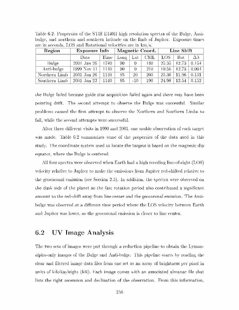
Table 6.2: Properties of the STIS E140H high resolution spectra of the Bulge, Anti-bulge, and northern and southern latitude on the limb of Jupiter. Exposure timesare in seconds, LOS and Rotational velocities are in km/s.
Region Exposure Info Magnetic Coord. Line Shift
Date Time Long Lat CML LOS Rot ∆λBulge 2001 Jan 26 1740 90 0 180 25.35 12.73 0.154
Anti-bulge 1999 Nov 11 1140 90 0 210 10.56 12.73 0.094Northern Limb 2001 Jan 26 1140 85 20 205 25.36 11.96 0.151Southern Limb 2001 Jan 23 1140 85 -10 190 24.98 12.54 0.152
the Bulge failed because guide star acquisition failed again and there may have been
pointing drift. The second attempt to observe the Bulge was successful. Similar
problems caused the rst attempt to observe the Northern and Southern Limbs to
fail, while the second attempts were successful.
After three dierent visits in 1999 and 2001, one usable observation of each target
was made. Table 6.2 summarizes some of the properties of the data used in this
study. The coordinate system used to locate the targets is based on the magnetic dip
equator, where the Bulge is centered.
All four spectra were observed when Earth had a high receding line-of-sight (LOS)
velocity relative to Jupiter to make the emissions from Jupiter red-shifted relative to
the geocoronal emission (see Section 2.5). In addition, the spectra were observed on
the dusk side of the planet so the fast rotation period also contributed a signicant
amount to the red-shift away from line center and the geocoronal emission. The Anti-
bulge was observed at a dierent time period where the LOS velocity between Earth
and Jupiter was lower, so the geocoronal emission is closer to line center.
6.2 UV Image Analysis
The two sets of images were put through a reduction pipeline to obtain the Lyman-
alpha-only images of the Bulge and Anti-bulge. This pipeline starts by reading the
clear and ltered image data les from one set as an array of brightness per pixel in
units of kiloRayleighs (kR). Each image comes with an associated almanac le that
lists the right ascension and declination of the observation. From this information,
256

Figure 6-2: The clear 25MAMA (left) and ltered F25SRF2 (right) images of Jupiterwith the Bulge on the limb. The o-planet (white) boxes show where the backgroundsky was subtracted. The on-planet (black) boxes show the region where the F25SRF2scaling factor was determined.
NASA's Navigation and Ancillary Information Facility (NAIF) can be used to derive
the location of the center of the planet. The program shifts the center of the planet
in the clear image so it is aligned with the center of the planet in the ltered image.
Both images are then rotated so Jovian north is pointing up. Figure 6-2 shows the
two images when the Bulge is on the limb.
Next, the sky background was subtracted in both images. A 100 x 100 pixel region
was dened near the edge of each image, shown in Figure 6-2 as the white box to the
left of the planet. The average brightness per pixel was calculated and subtracted
from the entire image.
Next, the intensity of the ltered image was scaled to that of the clear image. A
200 x 200 pixel region was dened near the center of each image, shown in Figure
6-2 as the black box near the right side of the image, and the average brightness per
pixel in the region was calculated. It is known that the average brightness of the
Lyman-alpha emission on the disc of the planet is about 8 kR. To account for the
dierence in sensitivities between the 25MAMA and F25SRF2 lters, a scaling factor
was calculated to use the known dierence in brightness on the disc between the two
images because of the lter and sensitivity and exposure time dierences. The scaling
257

factor S was dened as
S =AC − ALyα
AF(6.1)
where AC is the average brightness of the square in the clear image, ALya is the average
brightness of the Lyman-alpha emission (8 kR), and AF is the average brightness of
the square in the ltered image. The ltered image was then multiplied by this scaling
factor.
Finally, the Lyman-alpha image of Jupiter, shown in Figure 6-3, is obtained by
subtracting the scaled ltered image from the clear image. The darker diagonal line
that appears in each of the original images is an instrumental artifact caused by the
shadow of a repeller wire within the STIS instrument. The wire is designed to increase
the quantum eciency of the microchannel plate detector. Pixels on these lines were
disregarded during the analysis. The high noise levels seen on the disc result from
subtracting two large numbers. Larger variations in brightness are due to the planet
rotating between observations, so a brighter region would be overly subtracted and
dark in one spot and brighter in another in the Lyman-alpha-only image.
Next, the brightness across the limb as a function of latitude was found. First,
the location of the limb was calculated. Because Jupiter rotates so quickly, it is not
spherical, so the location of the limb as a function of latitude was calculated using
the known polar and equatorial radii. Then, the image was rotated at one degree
intervals between ±40 degrees latitude. At each line of latitude on the limb, a region
20 pixels tall that stretched across the entire length of the image was dened. Figure
6-4 shows an example of this process where the image rotated to 25 degrees latitude.
The yellow box outlines the 20 pixel tall region, and the black line near the center of
the box is the calculated 1-bar level of the cloud tops.
The averages and standard deviations of the vertical columns of each of these
regions were calculated and plotted as an intensity trace across the limb. An expo-
nential function was t from the peak intensity down to the rst point where the
brightness went below zero to calculate the scale height at each line of longitude.
258

Figure 6-3: Lyman-alpha image of Jupiter with the Bulge on the limb. See text foran explanation of the noise on the disc.
259

Figure 6-4: Example region on the limb at 25 degrees latitude dened to calculatethe brightness across the limb.
Figure 6-5 shows an example of an intensity trace across the equator. The white
line shows the average value of the pixels in each vertical column and the black regions
show the standard deviation. The red shaded region indicates the brightness within
±5 pixels from the peak brightness across each intensity trace. These values were
averaged to obtain the mean limb brightness at this longitude. The thin red line
indicates the best t exponential function to the brightness curve above the Lyman-
alpha peak.
The mean limb brightness was plotted as a function of latitude for both the Bulge
and Anti-bulge Lyman-alpha images, shown in Figure 6-6. The error bars indicate
the standard deviation in the calculation of the mean brightness, and the black data
points indicate the latitudes where the repeller wire interfered with the intensity trace
across the limb.
When the Bulge was observed, the magnetic equator is about 15-20 degrees north
of the rotational equator. The analysis shows that a peak in hot hydrogen brightness
occurs near 10-20 degrees north latitude, although the repeller wire limits the ability
260

Figure 6-5: Example plot of the intensity trace across 0 degrees latitude. The whiteline shows the average value of the pixels in each vertical column and the black regionsshow the standard deviation. The red shaded region shows the area where the meanlimb brightness was calculated and the thin red line indicates the best t exponentialfunction to the brightness curve.
Figure 6-6: Limb brightness as a function of latitude for the Bulge (left) and theAnti-bulge (right)
261
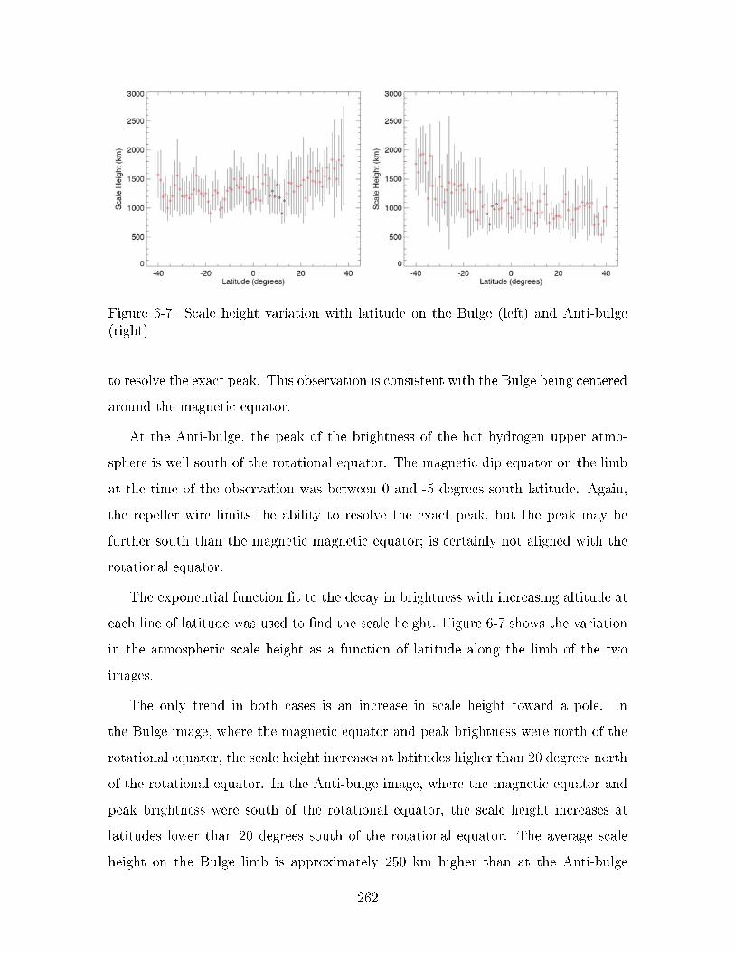
Figure 6-7: Scale height variation with latitude on the Bulge (left) and Anti-bulge(right)
to resolve the exact peak. This observation is consistent with the Bulge being centered
around the magnetic equator.
At the Anti-bulge, the peak of the brightness of the hot hydrogen upper atmo-
sphere is well south of the rotational equator. The magnetic dip equator on the limb
at the time of the observation was between 0 and -5 degrees south latitude. Again,
the repeller wire limits the ability to resolve the exact peak, but the peak may be
further south than the magnetic magnetic equator; is certainly not aligned with the
rotational equator.
The exponential function t to the decay in brightness with increasing altitude at
each line of latitude was used to nd the scale height. Figure 6-7 shows the variation
in the atmospheric scale height as a function of latitude along the limb of the two
images.
The only trend in both cases is an increase in scale height toward a pole. In
the Bulge image, where the magnetic equator and peak brightness were north of the
rotational equator, the scale height increases at latitudes higher than 20 degrees north
of the rotational equator. In the Anti-bulge image, where the magnetic equator and
peak brightness were south of the rotational equator, the scale height increases at
latitudes lower than 20 degrees south of the rotational equator. The average scale
height on the Bulge limb is approximately 250 km higher than at the Anti-bulge
262

limb. This is more evidence that the phenomena observed at the magnetic equator
are being inuenced by activity in higher latitudes.
The analysis of these Lyman-alpha images of the Jupiter limb provides strong
evidence that the center of brightness along the limb is not tied to the rotational
equator. The analysis also shows strong evidence that the center of brightness along
the limb is tied to the magnetic equator. There is also some supporting evidence that
activity along the magnetic equator is inuenced by higher latitudes.
6.3 Spectrum Analysis
6.3.1 Spectrum Reduction Pipeline
Data from the spectral observing campaign were downloaded from the Space Tele-
scope Science Institute (STScI), which stores data from all Hubble observations for
anyone to download and analyze. Unlike the images, the spectra need to be corrected
for distortions before they can be analyzed. The data are available in several dierent
forms that have some level of corrections, but for this analysis the raw data les were
put through an IDL reduction pipeline described here to obtain the reduced spectra
for data analysis. Figure 6-8 shows the raw data from the Bulge observation.
The raw data are represented in IDL as a 2048 x 2048 array with values corre-
sponding to individual photon counts recorded by the detector. This array is rst
shrunk to a 1024 x 1024 array that preserves the total counts but does not other-
wise change the data as it appears in Figure 6-8. The next step is to remove the
dark counts data from the raw data. The dark data le is taken from STScI and
multiplied by the exposure time then subtracted from the raw data to obtain the
dark-corrected data. The dierence between the raw and the dark-corrected data is
almost unnoticeable but is nevertheless important.
Next, at-eld corrections were implemented to correct for changing sensitivity
across the eld of view. There are two at eld corrections implemented in this
pipeline, low-order and pixel-to-pixel. The low-order at eld correction corrects for
263

Figure 6-8: Raw data for Hubble STIS spectral-spatial observation of the JupiterLyman-alpha Bulge
264

Figure 6-9: Low-order at eld (left) and pixel-to-pixel at eld (right) correctionsfor E140H data. Values on the low-order at eld range from 0.837 to 1.049. Valueson the pixel-to-pixel at eld range from 0.001 to 1.433.
variations in sensitivity of the optics in HST. The pixel-to-pixel at eld correction
corrects the spectrum for variations in the sensitivity in the detector. Figure 6-9 shows
both the low-order and at-eld corrections. Notice the hexagonal grid pattern in the
pixel-to-pixel at eld that corresponds to the detector's multichannel plate bundles.
Photons striking the edges of these bundles have a decreased probability of registering
a count in the detector.
These two at eld corrections are multiplied together to form the combined
at eld correction. The dark-corrected data is then divided by this combined at
eld correction to obtain the at eld corrected data. Both the combined at eld
correction and at eld corrected data are shown in Figure 6-10.
Notice that the strong line corresponding to the geocoronal emission running from
top to bottom of the data is not a straight line. This results from the echelle dispersion
and cross-dispersion. The properties of this dispersion are known from calculations
and previous observations and are used to regrid the at eld corrected spectrum so
that movement along a vertical line corresponds only to movement along the spatial
dimension. After the spectrum is regridded, the columns of the array do not change in
wavelength. Figure 6-11 shows the at eld corrected spectrum next to the regridded
265

Figure 6-10: Combined at eld data (left) and at eld corrected data (right). Valueson the combined at eld correction range from 0.001 to 1.353.
spectrum.
One nal correction is necessary before the spectrum can be analyzed. Dispersion
sensitivity varies perpendicularly to the wavelength axis. Like the properties of the
cross-dispersion, the properties of perpendicular dispersion sensitivity are known.
Figure 6-12 shows this sensitivity as a function of pixel location and as spectral data.
The regridded spectrum is divided by the dispersion sensitivity correction spectrum
to obtain the nal reduced spectrum, shown in Figure 6-13, which can be used for
data analysis.
6.3.2 Obtaining the Bulge Spectrum
The nal reduced spectrum shows Lyman-alpha echelle order 30 left of the center and
order 31 cut o on the right side. Order 30 is what was analyzed in this analysis (see
Section 2.6 for echelle basics and what the orders are). Figure 6-14 shows a zoomed
in view of the area of the spectrum that is of interest, the limb of the planet, and
labels some of the features that can be seen from inspection.
To obtain the spectrum from only the limb, the sky background must be sub-
tracted. An IDL routine had already been written to do this task, but it was modied
266

Figure 6-11: Flat eld corrected spectrum (left, same as Figure 6-10) and regriddedspectrum (right).
Figure 6-12: Perpendicular dispersion sensitivity correction plot (left) and equivalentspectral data (right).
267

Figure 6-13: Final reduced STIS spectrum of the Jupiter Lyman-alpha Bulge.
268

Figure 6-14: Zoomed-in view of the spectrum showing the limb in more detail.
269

Figure 6-15: Raw spectrum of the limb.
for this analysis to calculate uncertainty in the removal of the sky background. First,
the routine performs a horizontal intensity trace along a selected region. A horizontal
region 40 pixels wide shown by the yellow dotted lines in Figure 6-14 was chosen. The
brightness in each column is added and plotted as a function of wavelength. Figure
6-15 shows the spectrum that results from the intensity trace across the limb region.
Next, the routine selects a region of the sky background to subtract out of the
spectrum of the limb region. In most of the spectra, there is an area at least 250
pixels tall that can be used to obtain a sky background spectrum, and large regions
are better because of the reduced uncertainty in the total count rate compared to
smaller regions. An intensity trace is performed across the selected sky region, and all
the pixels in each column are added together and plotted as a function of wavelength.
Figure 6-16 shows the spectrum of the sky background.
The large peak at 1215.67 Å is the geocoronal background emission, and the area
on the right of the geocoronal peak that is brighter than the left side is emission from
the interplanetary medium (IPM).
The Poisson uncertainty, dened as the square root of the number of counts in
270

Figure 6-16: Sky background spectrum.
each wavelength bin, is calculated for both the raw spectrum and the sky background.
Then, the sky background is subtracted from the raw spectrum, resulting in the limb
spectrum. The uncertainty in the limb spectrum is also calculated as the square roots
of the sum of the squares of the raw and sky background uncertainties.
Figure 6-15 shows the resulting limb spectrum when the sky background is sub-
tracted from the raw spectrum. The spectrum was plotted again in Figure 6-18 using
an IDL smoothing function that alters the spectrum data on the plot for clarity. Sub-
sequent plots will also use this line smoothing technique, but all calculations described
hereafter are performed on the actual spectrum data and not the smoothed data.
The sky background appears to be oversubtracted in Figure 6-18. This is expected
because light from Jupiter at the same wavelength as the geocoronal hydrogen atoms
will be scattered by those atoms. Some light will be scattered by neutral hydrogen
in Earth's atmosphere. Another IDL routine was written to vary the intensity of the
sky background spectrum before it is subtracted from the raw spectrum and displays
a closer view of the corrected limb spectra. Figure 6-19 shows a closer view of the
limb spectrum with the sky background scaled to 92% of its original intensity before
271

Figure 6-17: Rough spectrum of the limb with the sky background subtracted.
Figure 6-18: Spectrum of the limb with an IDL smooth function applied.
272

Figure 6-19: Closer view of the limb spectrum with the adjusted background sub-traction. The solid line is the smoothed data and the dashed lines show ±1-sigmauncertainty with Poisson statistics.
it was subtracted. The Poisson error is also plotted with the spectrum. Notice the
higher relative error near 1215.65 Å where the sky was subtracted. This is a result of
error propagation and needs to be accounted for when modeling the spectrum.
6.3.3 Modeling the Hot and Cold Components
It is known that the broad spectrum in the Bulge is the result of a two-component
structure, one composed of cold neutral hydrogen and the other composed of super-
thermal hydrogen. The atmosphere in this region is optically thick, so a Voigt prole
will not provide an accurate t to the data (see Section 2.5). A full radiative transfer
model is the only way to model the entire spectrum. However, the super-thermal
(hot) hydrogen is a much smaller part overall and is optically-thin compared to the
cold component, so a Voigt prole can be t to the super-thermal component and
subtracted from the spectrum, leaving only the cold component.
A new IDL routine was written from scratch that ts a Voigt prole to the wings of
the spectrum using a least-squares tting algorithm. First, the bounds of the regions
273

Figure 6-20: Limb spectrum showing bounds on where the hot component Voigtprole was t.
Table 6.3: Range, step sizes, and initial guesses of the Voigt prole variables for thehot model t of the Bulge spectrum.
Variable Low High Step Size Initial Guess
Temperature (K) 200000 500000 2500 325000Line Center (Å) 1215.7 1215.9 0.005 1215.8Peak Brightness (R/Å) 10000 40000 100 30000
on both sides of the central peak of the spectrum are dened where the Voigt prole
will be t. Figure 6-20 shows these bounds on the limb spectrum.
Next, ranges of values and step sizes for the temperature, line center, and peak
brightness of the Voigt prole are dened. Table 6.3 lists the ranges and step sizes of
the variable used in the example shown.
The tting algorithm starts by xing the line center and peak brightness values
at the initial guesses and reading the lowest value of the temperature range. It builds
a Voigt prole for the hot hydrogen Lyman-alpha component of the spectrum and
convolves it with the STIS E140H line spread function (LSF). Then, the algorithm
linearly interpolates the Voigt prole to the same wavelength scale as the limb spec-
trum. A subroutine calculates the sum of the least squares of the dierence between
274

the values of the model and the data and reports the chi-squared value. This value is
stored and the temperature is increased by a step. This is repeated until the highest
temperature in the range has been used. The temperature with the lowest chi-squared
value is stored.
Next, the algorithm runs a second loop creating a Voigt prole, convolving it with
the E140H LSF, and nding the chi-squared value, but it xes the temperature at the
value that was found in the previous loop, sets the peak brightness equal to the initial
guess, and varies the line center. The line center that produces the lowest chi-squared
value is then used with the best t temperature from the rst loop as the starting
points for a third loop that sweeps the values of peak brightness.
These three loops are repeated, varying one variable while using the best guess of
the other two variables from the previous overall iteration, until the nal chi-squared
values converges to within 1x10⁻⁵. Convergence has occurred every time the algorithm
has been executed within 4 iterations. After the algorithm converges on a solution, the
best t values of the three variables are again used to create a Voigt prole convolves
with the E140H LSF and interpolated with the limb spectrum.
In an earlier version of this program, the three variables were not swept one at a
time, but all possible combinations of the three variables were used in a triple FOR
loop that calculated Voigt proles and found chi-squared values. This algorithm was
slow when the step size for the variables was small, which corresponds to a high
resolution t. It required a number of calculations on the order of O(n3) to nish,
where n is the number of values a variable could be within the dened range. It was a
brute force way to nd a solution, not a smart way. The new version of the algorithm
requires a number of calculations on the order of O(mn), where m is the number of
iterations required to reach convergence. Each of the three variables is swept once
per iteration, and a much higher resolution can be used to nd the best t in the
same time period.
After the best t model is found, it is subtracted from the limb spectrum. The
algorithm outputs the best t variables, the best t model, and the result from
subtracting the model from the data. Figure 6-21 shows the resulting Voigt prole of
275

requires
Figure 6-21: Voigt prole of the model hot component plotted with the limb spectrumand the remainder when the model is subtracted from the limb spectrum.
the hot component (solid line) plotted against the limb spectrum (dashed line). The
remaining spectrum (dotted-dashed line beneath the model) is the cold component,
which can be modeled using a similar algorithm.
The best t of the line center does not appear to be very sensitive to changes in
the bounds, but the other two variables are quite sensitive to where the boundaries of
the t are chosen. If the right boundary of the left side moves into the area where the
uncertainty is higher due to the subtraction of the sky, the chi-squared value of the
best t will be higher. If the left boundary of the right side is moved closer to the line
center, the dips caused by turbulence can cause the peak intensity to decrease and
the temperature to increase to compensate for the loss. If the bounds are too thin,
the peak intensity can overshoot the entire spectrum. Clearly, there are limitations
as to how well this algorithm ts the data because the Voigt prole is a simplied
but inaccurate way to model this complex area of Jupiter's atmosphere.
Just like with the hot component, the uncertainty must be considered when choos-
ing the boundaries to t a model of the cold component. On this spectrum, the
increased uncertainty from the sky is reaching into the left side of the cold peak, so
276

Figure 6-22: Remainder of the limb spectrum after the hot model spectrum wassubtracted showing bounds on where the cold component Voigt prole was t.
Table 6.4: Range, step sizes, and initial values of the Voigt prole variables for thecold model t of the Bulge spectrum. These values are not representative of the trueconditions because this simplied model does not take into account line broadeningeects caused by radiation transfer in an optically thick column of gas.
Variable Low High Step Size Initial Guess
Temperature (K) 10000 40000 100 25000Peak Brightness (R/Å) 20000 40000 100 30000
the right side is used more than the left for the model t. Figure 6-22 shows the
remaining cold component of the spectrum plotted with the uncertainty values and
the boundaries used to t a Voigt prole to the cold component.
Another algorithm was written from scratch that is very similar to the hot model
algorithm, but instead of tting all three variables required to generate a Voigt prole,
the line center is found rst using a peak-nding subroutine, so only the temperature
and peak intensity ranges need to be swept to nd a model with the best least squares
t. Table 6.4 shows the range, step size, and initial guesses used in the second least-
squares tting algorithm to model the cold component.
These bounds do not reect the actual conditions of the cold component of hy-
277

Figure 6-23: Voigt prole of the model hot component plotted with the remainder ofthe limb spectrum after the hot component was subtracted.
drogen; to gather a fully realistic set of bounds, a full radiative transfer model would
be needed to account for the line broadening. The articially high temperature given
here is what articially broadens the Voigt prole model so it ts the remainder of the
spectrum after the hot component has been subtracted out. Figure 6-23 shows the
cold component model plotted over what remained after the hot model was subtracted
from the Bulge limb spectrum with the bounds that the model is t to.
Finally, Figure 6-24 shows the combination of the hot and cold models plotted over
the data along with the values of the model parameters. As expected, the features
that show evidence of turbulence do not match the simplied model, but aside from
these bumps the overall shape ts the data well. Also as expected, the temperature
values used to broaden the Voigt proles are unrealistically high because optical depth
broadens the line proles.
An unexpected nding was the large dierence between the best t of the line
centers at the Bulge, marked by the two vertical lines in Figure 6-24. The hot com-
ponent's best t for the line center was red-shifted by 0.07 Å compared to the line
center of the cold component, which was in agreement with the predicted line center
278

Figure 6-24: Combined hot and cold models plotted against the original limb spec-trum. Vertical lines are the line centers of the two component models.
given the LOS velocity of Jupiter relative to Earth and rotational velocity of the limb.
This line center dierent corresponds to a velocity dierence of 16 km/s between the
hot component and the cold component. The spectral asymmetry had been noticed
in previous studies but was never formally calculated until now.
The data reduction, sky subtraction, and two-component model tting pipelines
described in this section were also applied to the other three spectra. Table 6.5 shows
the numerical results and Figure 6-25 shows the plots of all four spectra. The total
Lyman-alpha brightness was calculated by integrating the spectrum over 1.0625 Å
centered at the peak, large enough to capture the wings of the emission but not the
background noise left over after the sky subtraction. The values for temperature and
peak brightness of the cold component listed here also are not representative of the
true conditions because the simplied nature of the model.
In the regions north and south of the Bulge, there is a similar line separation
between the hot and cold components, but the corresponding velocity dierence is
a few kilometers per second less than at the Bulge. This is strong evidence that
the Bulge is inuenced by and possibly energized by the auroral regions. The hot
279

Table 6.5: Model outputs for all four limb spectra. The temperature and peak bright-ness values of the cold component do not represent accurate values because a fullradiative transfer analysis was not used in this model.
Bulge Anti-bulge Northern Southern
Total Spectrum Brightness 21.0 20.4 20.3 20.3Model OutputsHot ComponentTemperature (K) 337500 350000 330000 297500Line Center (Å) 1215.86 1215.79 1215.85 1215.84
Peak Brightness (kR/Å) 29.6 30.0 30.0 29.7Cold ComponentTemperature (K) 34000 9100 15000 25000Line Center (Å) 1215.79 1215.77 1215.80 1215.80
Peak Brightness (kR/Å) 26.2 29.7 28 30.2Velocity Dierence (km/s) 16.3 7.1 12.2 11.6
Figure 6-25: Combined hot and cold component ts to the spectra. (Top Left) Bulgelimb. (Top Right) Anti-bulge Limb. (Bottom Left) Northern Limb. (Bottom Right)Southern Limb.
280
and cold components of the Anti-bulge spectra have an even smaller line separation
compared to the Bulge, corresponding to a smaller velocity dierence between the
two components.
The modeled temperature in the hot component of the Bulge is higher than in
the regions to the north and south. However, the modeled temperature of the hot
component in the Anti-bulge is much higher than the other three spectra. This does
not agree with data from the image analysis (Section 6.2); the average scale height
at the Bulge was 250 km greater and therefore should have a higher temperature.
Upon closer inspection of Figure 6-25(top right), note that this spectrum looks
broader and therefore should have a higher temperature value for a Voigt prole.
The model hot component is also a much larger percentage of the whole spectrum
in the Anti-bulge, which may help explain why the model is not much less brighter
overall compared to the Bulge. See Section 6.3.4 for more on a possible reason why
the modeled temperatures of the hot components are lower than the Anti-bulge.
A caveat in this analysis is that the four observations were not all taken in the
same time period (see Table 6.2). The Anti-bulge spectrum was observed 14 months
prior to the other three spectra, and the Southern Limb spectrum was observed three
days prior to the Bulge and Northern Limb spectra. Previous studies have shown that
there are variations in the brightness of the Bulge that correspond to changes in the
Solar cycle [41]. The Solar Lyman-alpha ux on the day the Anti-bulge was observed
was approximately 10% stronger that it was during the time the Bulge, Northern,
and Southern Limbs were. The Anti-bulge is therefore brighter as a result.
In addition, the Anti-bulge spectrum was observed at a time when the LOS veloc-
ity between Jupiter and the Earth was lower than it was during the other observations.
The geocoronal emission spectrum was therefore closer to the line center of the Jupiter
data, and the relative error in the Voigt prole model tting was higher.
Furthermore, the lower LOS velocity between Jupiter and Earth makes the sky
subtraction in Anti-bulge more dicult. Choosing dierent parameters for the strength
and shift in the sky background before it is subtracted from the raw spectrum changes
the nal output of the model. Given one set of parameters, the line shift between the
281

hot and cold models can correspond to a velocity dierence as low as 0 km/s or as high
as 10 km/s. Also, because the Solar Lyman-alpha ux was higher, the geocoronal
and IPM emissions were also brighter, bringing the total error in the model ttings
even higher. Use of a comprehensive radiative transfer model could more accurately
subtract the sky background so that this model could more accurately calculate the
line separation and the relative velocity between these two components.
6.3.4 Optical Depth and Column Density Analysis
Even though the overall optical depth of the hydrogen in the spectra is too high to
calculate the column density without requiring a complex radiative transfer model
to account for multiple scattering, a simplied analysis can be performed on the hot
component because the wings of the line are optically thin. In an optically thin gas
(τ = 1), it can be assumed that photons are scattered by only one atom (single
scattering) and brightness is directly proportional to the column density of atoms
along the line of sight. The following analysis to calculate the column density of the
hot population of neutral hydrogen atoms in the Jupiter spectra is based on R.R.
Meier's work [43] for a single scattering radiative transfer from Solar Lyman-alpha
light.
The column density can be calculated by
N =B
g(6.2)
where N is the number density of hydrogen along a column, B is the total brightness
of the measured emission, and g is the Solar g-factor. The Solar g-factor is dened
as the numbers of photons per second an atom will produce from reecting Solar
radiation and is calculated as
g = (πFS√π∆λD)σ0 (6.3)
where πFS is the Solar ux in photons per square centimeter per second per Angstrom,
∆λD is the Doppler width with respect to wavelength, and σ0 is the resonant scat-
282

tering cross section of hydrogen at line center. This formula assumes constant Solar
ux at all wavelengths and constant scattering cross section, both of which are good
assumptions when the Lyman-alpha spectral line prole is thin compared to the Solar
Lyman-alpha prole. In the case of the Jupiter Bulge, however, this is not true. The
Jupiter line prole is very broad, so the variations in the Solar Lyman-alpha ux
and the scattering cross section must be accounted for. A more general case of the
Solar g-factor equation will be developed later in this section to solve for the column
density.
Figure 6-26 shows a model of the Solar Lyman-alpha ux at Jupiter and the
model Voigt prole of the hot component of the Bulge found in Section 6.3.3. The
Solar prole is centered at the rest wavelength of Lyman-alpha (1215.67 Å) and
the hot component model is centered at the best t line center found in the tting
algorithm, which was shown to be even more red-shifted from the line center than if
only planetary rotation was causing a line shift.
Two observations are signicant in this gure. First, notice that the Solar Lyman-
alpha ux is not constant across all wavelengths. The dip in the center is due to
resonant scattering by colder hydrogen gas in the Solar atmosphere, but light further
from line center is brighter per unit Angstrom on both sides. Clearly, the change in
the Solar ux at dierent wavelengths must be accounted for.
Second, notice how wide the hot component model is compared to the Solar prole.
Both proles are nearly 1 Angstrom wide, and both proles decay at similar rates
at higher wavelengths (right side of the graph). This means there could be more
hydrogen moving at greater speeds relative to the planet, but there is simply no Solar
Lyman-alpha ux at those wavelengths for the hydrogen to reect. This possibility
will be revisited later in this section.
The resonant scattering cross section of neutral hydrogen is dependent on tem-
perature and wavelength. An advantage of the Voigt prole is that it shows how the
scattering cross section varies with wavelength relative to the cross section at line
center. The cross section at line center varies inversely with the square root of the
temperature, or σ ∝ T 1/2. The scattering cross section in the hot component can be
283

Figure 6-26: Model Solar Lyman-alpha ux at Jupiter (solid line) plotted over the hotcomponent spectrum model (dotted line). Notice the Solar Lyman-alpha ux is di-minished in the center because of scattering by colder atoms in the Solar atmosphere,so there are two peaks.
284

Figure 6-27: Resonant scattering cross section of the model hot component.
calculated using a known value at a given temperature. Wiese et al. [57] measured
a scattering cross section of neutral hydrogen at 1000 K of 1.865 x 10⁻¹³ cm2. The
scattering cross section in the hot component was calculated by
σTBF= σ1000K
√1000
TBF(6.4)
where σ1000K is the cross section at 1000 K and TBF is the best t temperature of the
Voigt prole of the hot component. The cross section at line center can be used to
scale the Voigt prole to model how scattering cross section changes with wavelength,
shown in Figure 6-27.
Now the Solar g-factor per Angstrom can be found with
g(λ)dλ =√π · πF (λ) · σ(λ)dλ (6.5)
Figure 6-28 shows g(λ)dλ. The curve is skewed to the right because the hot
285

Figure 6-28: Solar g-factor as a function of wavelength.
Table 6.6: Results from the column density analysis of the hot component of thespectra.
Model Outputs Bulge Anti-Bulge Northern SouthernScattering Cross Section (cm2) 1.03 x 10⁻¹⁴ 9.97 x 10⁻¹⁵ 1.03 x 10⁻¹⁴ 1.08 x 10⁻¹⁴
Solar G-Factor (photons/s-atom) 1.08 x 10⁻⁴ 1.10 x 10⁻⁴ 1.09 x 10⁻⁴ 1.11 x 10⁻⁴
Column Density (atoms/cm2) 1.46 x 10¹⁴ 1.50 x 10¹⁴ 1.46 x 10¹⁴ 1.35 x 10¹⁴
component peak matches closely with the right peak of the Solar Lyman-alpha ux.
When g(λ)dλ is integrated, the result is the Solar g-factor. When the hot com-
ponent model is integrated, the result is the total brightness of the hot component.
The column density is the brightness divided by the Solar g-factor. Table 6.6 shows
the results from this process applied to all four spectra.
The scattering cross-sections are on the order that was expected when compared
to the value reported by Wiese et al. [57] and considering the high temperature. The
values of the Solar g-factor are also comparable given the increased distance from the
Sun and lower Solar Lyman-alpha ux. The column density calculated in the Bulge
286

Figure 6-29: Comparison of the Solar g-factor function in the Bulge (left) and Anti-bulge (right) spectra.
region atmosphere is consistent with estimates made by Emerich et al. [11].
The higher calculated column density in the Anti-bulge atmosphere compared
to the Bulge atmosphere can be explained by the red-shift of the hot components
relative to the expected values. Figure 6-29 shows the Solar g-factor as a function of
wavelength in the Bulge and Anti-bulge spectra. Because the hot component of the
Anti-bulge is closer to the line center of the Solar Lyman-alpha ux, more photons
on the blue-shifted peak left of the center (see Figure 6-26) are being scattered by the
hot atoms on the blue-shifted wing of the hot component. Since there are more Solar
Lyman-alpha photons that can be scattered by these atoms, it results in a higher
calculated column density.
This could also explain why the temperature calculated in the model was higher in
the Anti-bulge than in the Bulge. Because of the high red-shift of the hot component
in the Bulge, not as many atoms were able to reect Solar Lyman-alpha light. Figure
6-26 shows that the red-shifted edge of the hot model is further away from the red-
shifted edge of the Solar Lyman-alpha prole. This could be an indication that there
are more hot atoms than what was calculated here traveling at higher speeds around
the planet. These would not be seen because they do not scatter Solar Lyman-alpha
light. In contrast, the Anti-bulge hot component is closer to the Solar Lyman-alpha
line center and can scatter more light.
If there were in fact more hot atoms moving at higher relative velocity to the cold
287

atoms in the Bulge, the distribution would have a broader model spectrum because
of the higher Voigt temperature. If the temperature is increased by an order of
magnitude in the column density analysis, the column density changes by a factor
less than two. There may be much more happening in Lyman-alpha Bulge of Jupiter
that has not been observed.
6.4 Discussion of Results
In summary, the results from the analyses of the images and spectra have shown:
1. The center of brightness in Lyman-alpha along the limb of the planet is aligned
with the magnetic equator, not the rotational equator.
2. The emission scale height of higher latitudes on the hemisphere that is closer
to the magnetic equator is higher than the emission scale height of the other
hemisphere (see Figure 6-7).
3. The average scale height of the limb of the planet when the Bulge is on the limb
is 250 km higher than the average scale height of the limb when the Anti-bulge
is on the limb.
4. All four spectra qualitatively show evidence of turbulence. Turbulence causes
the line prole to increase outside of line center, creating the bumps seen on
the sides of the line center peaks in Figure 6-25.
5. All four spectra have broad, superthermal components that are red-shifted rel-
ative to the center of the peak emission, corresponding to velocity dierences
between the hot and cold components ranging from 16.3 km/s in the Bulge to
7.1 km/s in the Anti-Bulge.
6. The Northern and Southern limb spectra show lower velocity dierences between
the hot and cold components than the velocity dierence between the hot and
cold components at the Bulge.
288

7. The Bulge Lyman-alpha line prole is broader than the Northern and Southern
limbs as indicated by the best t temperature of the hot component model.
8. The spectral width of the hot components are comparable to the Solar Lyman-
alpha prole, indicating that there could be more neutral hydrogen moving at
higher speeds that is simply not scattering the Solar Lyman-alpha emission.
9. The column densities of the superthermal components of all four regions are
comparable.
The alignment of the peak limb brightness with the magnetic equator is evidence
that supports both the equatorial electrojet and the charged particle motion along
magnetic led lines hypotheses. Since the aurorae are not aligned with the rotational
axis of the planet, is is possible for a neutral high altitude jet from the aurora moving
from high latitudes to low latitudes to brighten the entire magnetic equator and make
one side even brighter..
The equatorial electrojet argument is further strengthened by the presence of
a broad spectral component on the Anti-bulge side of the planet and by the large
velocity dierence between the hot and cold components observed on both sides of
the planet. Again, depending on how the observed neutral winds from high latitudes
move to lower latitudes and interact with the equatorial electrojet, this could the
brightness of the magnetic equator to vary with longitude.
The increase in scale height in the higher latitudes near the magnetic equator is
evidence that the temperature in these regions are higher. This could be inuence
from the aurorae. However, it is not certain whether this is caused by neutral high
altitude jets or by charged particles moving down magnetic eld lines. Either scenario
would produce collisions in the upper atmosphere that would produce a Lyman-
alpha emission. This emission would also be present on the night side of the planet
due to scattering of the interplanetary emission, which is consistent with previous
observations from Voyager [4].The increased scale height could be a sign that an
equatorial electrojet is encountering more resistance as the magnetic equator peaks
relative to the rotational equator.
289

The dierence in the average emission scale height measured across the entire
limb between the Bulge and Anti-bulge images corresponds to a temperature increase
of 25% on the Bulge side compared to the Anti-bulge, since emission scale height
increases linearly with temperature. The actual temperature cannot be calculated
without a full radiative transfer analysis.
The hot component of the Bulge is moving more than 16 km/s faster than the
atmosphere below it. For context, the rotational speed of the planet at the equator
is approximately 12.5 km/s and the orbital speed at the exobase is approximately 40
km/s. This means the average superthermal hydrogen atom is moving at over half of
the remaining the speed required to achieve orbit. This can easily explain why such
a broad superthermal component exists at the Bulge and still has a high velocity
separation from line center; such a large amount of the hydrogen could be traveling
on suborbital trajectories that would take some of the atoms to the other side of the
planet.
Additionally, because the Doppler broadening causes the spectral prole to be so
broad, a large percentage of the hot component has enough energy to escape from
Jupiter entirely. The hot component's Voigt prole at the Bulge showed that 27%
of the hot emission was shifted such that its velocity was more than 60 km/s, which
exceeds the escape speed of Jupiter.
The high velocity dierence in the Bulge is much higher than what was observed
in the aurorae [15]. Even if both auroral regions were contributing hydrogen at 5
km/s, which is higher than what was observed by Rego et al., this would not be
enough to generate a high enough velocity to match the spectral separation observed
in the Bulge.
However, the Rego et al. observations measured jets near the homopause. The
pressure and density are orders of magnitude higher, so moving mass at high speeds
is much more dicult. It is still possible that hydrogen higher in the atmosphere
could be moving faster than the jets at lower altitudes.
The dierence in velocity between the Bulge and the Northern and Southern limbs
is consistent with friction causing the hydrogen to slow down more further from the
290

magnetic equator, as would be in the case of an equatorial electrojet. Alternatively,
these higher velocities could be explained by matter from higher latitudes gradually
colliding and changing from a north-south orientation to a westward direction, but
this seems unlikely because the pressure is too low to transfer momentum gradually.
Additionally, the Coriolis Force is strong and such changes would happen quickly.
Although the most published theory was that the turbulence inside the Bulge
region was being caused by activity in the poles of Jupiter, this study shows evidence
that activity along the magnetic equator may be responsible for the added brightness
of the Bulge. It is not conclusive evidence, however, but it does add to the body
of knowledge regarding the Bulge and the magnetic equator of Jupiter by describing
characteristics that have not been reported otherwise.
Because of the problems with the spectral data, and because the spectral data
cover such a limited range of Jupiter, it would be better to have more data with
fewer complications than the present spectra. Whether or not a follow-on study was
planned is unknown, but in August 2004, a failure in the STIS power system caused
STIS to be inoperable, so no more high-resolution spectral data could be recorded.
However, STIS was repaired during Servicing Mission 4 in May 2009, so a follow-on
study could now be proposed.
If a future Hubble campaign was proposed to improve upon this data, additional
spectral data sets from higher latitudes along the Bulge limb and at more points
along the magnetic equator would be desirable. In this campaign, there is only one
image and one spectrum each of the Bulge and Anti-bulge. Additionally, the latitudes
sampled in the regions above and below the Bulge are not far enough away to examine
what could be happening at mid-latitudes.
Additional spectra of the limb of the planet at higher latitudes would reveal
whether there is any western motion at higher latitudes; if the Bulge is being en-
ergized by the poles, the relative motion would be north/south and would not create
any red-shifting like what is seen in the spectral data from this campaign.
More spectra from around the magnetic equator would help characterize the fast
hydrogen moving around the planet. If the velocity of the superthermal component
291

at longitudes near ~200 degrees is in between what was measured at the Bulge and
Anti-bulge, and if the velocity of the superthermal component at longitudes near ~20
degrees is less than what is measured at the Anti-bulge, this would be an indication
that equatorial electrojets are not inuencing the Bulge. Equatorial electrojets would
instead be weakest at the Anti-bulge and stronger in the regions in between the Bulge
and Anti-bulge, climaxing at the Bulge.
292

Chapter 7
Conclusions
VeSpR was originally scheduled for ight in July 2010, but because of delays at
Wallops Flight Facility, the payload was not ready for integration testing and launch
before the launch window closed. Because of the low dierence in orbital periods
between Venus and Earth, potential launch windows are over a year and a half apart,
corresponding to dates when Venus will have a high incoming line-of-sight velocity.
As described in Section 5.5, the next launch window is in early 2012.
The year and a half delay in the launch date relaxed deadlines for new parts that
were being fabricated in the BU Scientic Instruments Facility. Other BU rocket
programs that required machine shop time received priority over VeSpR, so the fab-
rication of many of the parts described in Section 5.3 was delayed by several months.
This caused fabrication of the ight wiring harnesses to be delayed, which in turn
caused the testing of the new XDL detectors to be delayed past the point when the
test results could be included in Chapter 5.
VeSpR is now far ahead of schedule for a 2012 launch. With additional payload
testing at Wallops now scheduled for March 2011 and full payload integration and
testing scheduled for the summer, VeSpR should have no problems launching during
the next available launch window. Until then, the science team will be testing the
systems in vacuum and troubleshooting the ground support equipment.
Addition upgrades will be made to the VACTEF to prepare the facility for future
testing of spaceight hardware. The Mars Atmosphere and Volatile Evolution Mis-
293

sion, or MAVEN, will require components that must be tested in vacuum at lower
wavelengths than what is currently available for testing. Plans are already underway
to install a new monochromator in the vacuum chamber that is capable of testing
optics at much lower wavelengths than is currently available in the VACTEF. Over
the next six months, work on this project will start as other work on VeSpR will
continue as planned.
Meanwhile, the analysis of the raw data from the Jupiter Lyman-alpha Bulge is
complete. The results presented here will be compared with existing radiative transfer
models to see if the spectral data matches the model's output, but the conclusions
from this study may be used to further strengthen the validity of the model. As of
this writing, model proles are being constructed that can be compared to the data.
Additionally, now that STIS has been repaired, there is an opportunity to observe
the Bulge with Hubble again. The deadline for proposals for the next Hubble cycle is
at the end of February 2011. If the radiative transfer model's output cannot be recon-
ciled with the data from the 1999 and 2001 observations, there would be a strong case
to submit a proposal for Hubble observation time. If another Hubble campaign was
accepted, it would have stricter requirements on the observation windows and include
blue-shifted observations on the day side in addition to red-shifted observations on
the night side.
While these two projects were not strongly related on a technical level aside from
the design of the spectrograph instruments, the experience working on two very dier-
ent realms within space science has essentially condensed the lifecycle of a large-scale
space science operation into a timeframe that made it possible to complete a Mas-
ter's degree. Work on the pre-launch phase of VeSpR and the post-processing phase
of the Bulge data was happening concurrently so the author could experience both
the engineering build-up of a space mission and the scientic analysis of the raw data.
It is especially important for systems engineers to understand the big picture.
While most systems engineers are intimately familiar with the design of spacecraft
components and the emergent behaviors that arise in complex systems, not all of them
have worked with the nal results from the spacecraft and have an intimate knowledge
294

of the needs of the scientists who receive the nal data from the spacecraft. The
combination of the two projects here involved the design of single parts, tracking of
emergent behaviors of complex spacecraft systems, modeling the hardware to generate
expected results, and reducing data from an actual spacecraft in a similar way that
the VeSpR science team will do after launch.
295

296

Bibliography
[1] P. Z. Takacs B. R. Sandel D. E. Shemansky J. B. Holberg J. M. Ajello S. K.
Atreya T. M. Donahue J. L. Bertaux J. E. Blamont D. F. Strobel J. C. McConnell
A. Dalgarno R. Goody M. B. McElroy A. L. Broadfoot, M. S. Belton. Extreme
ultraviolet observations from voyager 1 encounter with jupiter. Science, 204:979
982, June 1979.
[2] C. W. Bowers S. Kraemer M. E. Kaiser A. C. Danks J. F. Grady J. J. Loiacono M.
Brumeld L. Feinburg T. R. Gull S. R. Heap S. P. Maran D. Linder D. Hood. W.
Meyer C. VanHouten V. Argabright S. Franka R. Bybee-D. Dorn M. Bottema
R. Woodru H. Garner J. G. Timothy M. Blouke C. L. Joseph G. Hartig R.
F. Green E. B. Jenkins J. L. Linsky J. B. Hutchings H. W. Moos A. Boggess
F. Roesler D. Weistrop B. E. Woodgate, R. A. Kimble. The space telescope
imaging spectrograph design. Publications of the Astronomical Society of the
Pacic, 110:11831204, October 1998.
[3] A. L. Broadfoot J. L. Bertaux J. E. Blamont M. J. S. Belton J. M. Ajello J. B.
Holberg S. K. Atreya T. M. Donahue H. W. Moos D. F. Strobel J. C. McConnell
A. Dalgarno R. Goody M. B. McElroy P. Z. Takacs B. R. Sandel, D. E. Sheman-
sky. Extreme ultraviolet observastions from voyager 2 encounter with jupiter.
Science, 23:962 966, November 1979.
[4] D. F. Strobel B. R. Sandel, A. L. Broadfoot. Discovery of a longitudinal asym-
metry in the h lyman-alpha brightness of jupiter. Geophysical Research Letters,
7(1):58, January 1980.
297

[5] Charles A. Barth. Interpretation of the mariner v lyman alpha measurements.
Journal of Atmospheric Sciences, 25:564567, July 1968.
[6] Chin-Ping Liu Mohammed Bahou Yuan-Pern Lee Yuk L. Yung M. F. Gerstell
Bing-Ming Cheng, Eh Piew Chew. Photo-induced fractionation of water iso-
topomers in the martian atmosphere. Geophysical Research Letters, 26(24):3657
3660, December 1999.
[7] Dale A. Ostlie Bradley W. Carroll. An Introduction to Modern Astrophysics.
Addison Wesley, 2 edition, 2007.
[8] H. A. Weaver J. A. McClintock C. B. Opal, P. D. Feldman. Two-dimensional
ultraviolet imagery with a microchannel-plate/resistive-anode detector. Proceed-
ings of the International Society of Optics and Photonics (SPIE): Instrumenta-
tion in astronomy III, 172:317320, 1979.
[9] Tobias Owen David Crisp Jean-Pierre Maillard-Barry L. Lutz Catherine de
Bergh, Bruno Bézard. Deuterium on venus: Observations from earth. Science,
251(4993):547549, February 1991.
[10] Kenneth K. Kelly Lloyd Wallace William G. Fastie Charles A. Barth, Jerey
B. Pearce. Ultraviolet emission observed near venus from mariner v. Science,
158(3809):16751678, December 1967.
[11] John T. Clarke Renée Prangé G. Randall Gladstone Joel Sommeria
Gilda Ballester Claude Emerich, Lot Ben Jael. Evidence for supersonic turbu-
lence in the upper atmosphere of jupiter. Science, 273(5278):10851087, August
1996.
[12] John T. Clarke Y. Kim G.E. Ballester R. Prangé J. Sommeria Claude Emerich,
Lot Ben Jael. Hot hydrogen belt detected with ly-a high resolution obser-
vations of jovian atmosphere. Bulletin of the American Astronomical Society,
32(DPS Meeting 32):1641, 2000.
298

[13] John T. Clarke Y. Kim G.E. Ballester R. Prangé J. Sommeria Insti-
tut d'Astrophysique Spatiale Team Institut d'Astrophysique de Paris Team
Claude Emerich, Lot Ben Jael. Hot atomic hydrogen in the upper jovian
atmosphere conrmed with ly-a high resolution stis observations. Bulletin of the
American Astronomical Society, 33(DPS Meeting 33):1067, 2001.
[14] D. McCoy J.-P. Lebreton S. Barabash J.-L. Bertaux P. Drossart V. Formisano
B. Haeusler O. I. Korablev W. Markiewicz D. Neveance M. Petzold G. Piccioni
T. L. Zhang F. W. Taylor E. Lellouch D. Koschny O. Witasse M. Warhaut A.
Acomazzo J. Rodrigues-Cannabal J. Fabrega T. Schirmann A. Clochet M. Cora-
dini D. V. Titov, H. Svedhem. Venus express: Scientic goals, instrumentation,
and scenario of the mission. Cosmic Research, 44(4):334348, 2006.
[15] Tom Stallard Steve Miller-Renee Prange Michele Dougherty Robert D. Joseph
Daniel Rego, Nicholas Achilleos. Supersonic winds in jupiter's aurorae. Nature,
399:121124, May 1999.
[16] William G. Fastie. A small plane grating monochromator. Journal of the Optical
Society of America, 42(9):641647, September 1952.
[17] D. Mugglestone G. D. Finn. Tables of the line broadening function h(a,v).
Monthly Notices of the Royal Astronomical Society, 129:221235, 1965.
[18] J. R. Barry G. J. Rottman, H. W. Moos. Lyman-alpha emission from arcturus.
The Astrophysical Journal, 165:661664, May 1971.
[19] G. J. Rottman H. W. Moos. Oi and hi emissions from the upper atmosphere of
venus. The Astrophysical Journal, 169:L127L130, November 1971.
[20] J. R. Barry J. L. Buckley H. W. Moos, R. C. Vitz. Small lif prism spectrometer
for space applications. Applied Optics, 9(3):601603, 1970.
[21] George R. Harrison. The production of diration gratings: Ii. the design of
echelle gratings and spectrographs. Journal of the Optical Society of America,
39(7):522528, July 1949.
299

[22] Eugene Hecht. Optics. Addison Wesley, 4 edition, 2002.
[23] Jack J. Lissauer Imke de Pater. Planetary Sciences. Cambridge University Press,
2 edition, August 2001.
[24] R. R. Hodges J. H. Homan. Composition of the venus lower atmosphere
from the pioneer venus mass spectrometer. Journal of Geophysical Research,
85(A13):78827890, December 1980.
[25] C. S. Freer H. W. Moos J. W. Giles, W. R. McKinney. An image-stabilized
telescope - ten channel ultraviolet spectrometer for sounding rocket observations.
Space Science Instrumentation, 1:5159, February 1975.
[26] Franck Montmessin Jean-Loup Bertaux. Isotopic fractionation through water
vapor condensation: The deuteropause, a cold trap for deuterium in the at-
mosphere of mars. Journal of Geophysical Research, 106(E12):32,87932,884,
December 2001.
[27] John T. Clarke Jean-Loup Bertaux. Deuterium content in the venus atmosphere.
Nature, 338:567568, April 1989.
[28] O. Korablev E. Villard E. Quemerais E. Neefs F. Montmessin F. Leblanc J.-P.
Dubois E. Dimarellis A. Hauchecorne F. Lefevre P. Rannou J. Y. Chaufray M.
Cabane G. Cernogora G. Souchon F. Semelin A. Reberac E. Van Ransbeek S.
Berkenbosch R. Clairquin C. Muller-F. Forget F. Hourdin O. Talagrand A. Rodin
A. Fedorova A. Stepanov I. Vinogradov A. Kiselev Yu. Kalinnikov Georges Durry
B. Sandel A. Stern J. C. Gerard Jean-Loup Bertaux, D. Nevejans. Spicav on
venus express: Three spectrometers to study the global structure and compo-
sition of the venus atmosphere. Planetary and Space Sciences, 55:16731700,
2007.
[29] Oleg Korablev E. Villard A. Fedorova D. Fussen E. Quemerais D. Belyaev-A.
Mahieux F. Montmessin C. Muller E. Neefs D. Nevejans V. Wilquet J. P. Dubois
A. Hauchecorne A. Stepanov I. Vinogradov A. Rodin the SPICAV/SOIR Team
300

Jean-Loup Bertaux, Ann-Carine Vandaele. A warm layer in venus' cryosphere
and high-altitude measurements of hf, hcl, h2o and hdo. Nature, 450:646649,
November 2007.
[30] J. Hunter Waite Jr. John T. Clarke, John Trauger. Doppler shifted h ly-a emis-
sionfrom jupiter's aurora. Geophysical Research Letters, 16(6):587590, June
1989.
[31] Lot Ben Jael John T. Clarke, G. Randall Gladstone. Jupiter's dayglow h ly-a
emission line prole. Geophysical Research Letters, 18(11):19351938, November
1991.
[32] P. D. Feldman H. W. Moos W. G. Fastie John T. Clarke, H. A. Weaver. Spa-
tial imaging of hydrogen lyman alpha emission from jupiter. The Astrophysical
Journal, 240:696701, September 1980.
[33] Paul D. Feldman John T. Clarke, H. Warren Moos. Iue monitoring of the spatial
distribution of the h ly-a emission from jupiter. The Astrophysical Journal,
245:L127129, May 1981.
[34] T. Owen A. Nagy John T. Clarke, Jean-Loup Bertaux. Hst/stis observations of
the extended martian upper atmosphere. Bulletin of the American Astronomical
Society, 36:1182, 2004.
[35] Anton Tremsin Oswald Siegmund John Vallerga, Jason McPhate. The current
and future capabilities of mcp based uv detectors. Journal of Astrophysical
Science, 320:247250, May 2009.
[36] Bruce Fegley Jr. Katharina Lodders. The Planetary Scientist's Companion. Ox-
ford University Press, 1998.
[37] Charles F. Hall Lawrence Colin. The pioneer venus program. Space Science
Reviews, 20:283306, 1977.
301

[38] A. Vidal-Madjar Lot Ben Jael, C. Magnan. The lyman alpha albedo of jupiter.
Astronomy and Astrophysics, 204(E12):319326, December 1988.
[39] John T. Clarke Lot Ben Jael, Y. J. Kim. The h lyman-alpha emission line
from the upper atmosphere of jupiter: Parametric radiative transfer study and
comparison with data. Icarus, 190:504527, April 2007.
[40] Renee Prange G. Randall Gladstone Alfred Vidal-Madjar Lot Ben Jael, John
T. Clarke. The lyman alpha bulge of jupiter: Eects of a non-thermal velocity
eld. Geophysical Research Letters, 20(8):747750, April 1993.
[41] H. W. Moos M. A. McGrath, G. E. Ballester. Jovian h2 dayglow emission (1978-
1989). Journal of Geophysical Research, 95(A7):10,36510373, July 1990.
[42] H. W. Moos M. Bottema, W. G. Fastie. A rocket telescope spectrometer with
high precision pointing control. Applied Optics, 8(9):18211826, September 1969.
[43] R.R. Meier. Ultraviolet spectroscopy and remote sensing of the upper atmo-
sphere. Space Science Reviews, 58:1185, 1991.
[44] Donald M. Hunten Michael B. McElroy. The ratio of deuterium to hydro-
gen in the venus atmosphere. Journal of Geophysical Research, Space Physics,
74(7):17201739, April 1969.
[45] Jose M. Rodriguez Michael B. McElroy, Michael J. Prather. Escape of hydrogen
from venus. Science, 215(4540):16141615, March 1982.
[46] J. Bixler S. Chakrabarti J. Vallerga S. Bowyer R. F. Malina O. H. W. Siegmund,
M. Lampton. Wedge and strip image readout systems for photon-counting detec-
tors in space astronomy. Journal of the Optical Society of America, 3:21392145,
December 1986.
[47] J. M. Grebowsky H. G. Mayr R. E. Hartle, T. M. Donahue. Hydrogen and deu-
terium in the thermosphere of venus: Solar cycle variations and escape. Journal
of Geophysical Research, 101(E2):45244538, February 1996.
302

[48] Laurent Pallier Lot Ben Jael Claude Emerich Joe Ajello John T. Clarke Gilda
E. Ballester Renee Prange, Daniel Rego. Detection of self-reversed ly-a line from
the jovian aurorae with the hubble space telescope. The Astrophysical Journal,
484:L169L193, August 1997.
[49] François Robert. Solar System Deuterium/Hydrogen Ratio, chapter 17, pages
341351. University of Arizona Press, 2006.
[50] Barbara Ryden. Introduction to Cosmology. Addison Wesley, 2003.
[51] Agustin Sanchez-Lavega. An Introduction to Planetary Atmospheres. Taylor and
Francis, 2011.
[52] Jean Schneider. The extrasolar planets encyclopaedia. Online
[http://exoplanet.eu/], February 1995. Accessed January 21, 2010.
[53] R. R. Hodges A. J. Watson T. M. Donahue, J. H. Homan. Venus was wet: A
measurement of the ratio of deuterium to hydrogen. Science, 216(4546):630633,
May 1982.
[54] John R. Taylor. An Introduction to Error Analysis: The Study of Uncertainties
in Physical Measurements. University Science Books, 2 edition, 1997.
[55] David A. Vallado. Fundamentals of Astrodynamics and Applications. Microcosm
Press and Klumer Academic Publishers, 2 edition, 2001.
[56] G. Randall Gladstone Vladimir A. Kransnopolsky, Michael J. Mumma. Detection
of atomic deuterium in the upper atmosphere of mars. Science, 280:15761580,
June 1998.
[57] B. M. Glennon W. L. Wiese, M. W. Smith. Atomic Transition Probabilities,
volume 1. U.S. Government Printing Oce, 1966.
[58] John W. Caldwell Paul D. Feldman Brett C. Bush Daniel M. Cotton
Supriya Chakrabarti Walter M. Harris, John T. Clarke. High-resolution ultravi-
303

olet spectrograph for sounding rocket measurements of planetary emission line
proles. Optical Engineering, 32(12):30163027, December 1993.
[59] Joseph Ladislas Wiza. Microchannel plate detectors. Nuclear Instruments and
Methods, 162:587601, 1979.
304


