Spectral Methods for the Calculation of Risk Measures for Variable

Annuity Guaranteed Benefits

Runhuan Feng

Department of Mathematics

University of Illinois at Urbana-Champaign

rfeng@illinois.edu

Hans W. Volkmer

Department of Mathematical Sciences

University of Wisconsin - Milwaukee

volkmer@uwm.edu

Abstract

Spectral expansion techniques have been extensively exploited for the pricing of exotic op-

tions. In this paper, we present novel applications of spectral methods for the quantitative risk

management of variable annuity guaranteed benefits such as guaranteed minimum maturity

benefits and guaranteed minimum death benefits. The objective is to find efficient and accurate

solution methods for the computation of risk measures, which is the key to determining risk-

based capital according to regulatory requirements. Our example calculations show that two

spectral methods used in this paper are highly efficient and numerically more stable than con-

ventional known methods. Hence these approaches are more suitable for intensive calculations

involving death benefits.

Key Words. Variable annuity guaranteed benefit, Asian option, risk measures, value at

risk, conditional tail expectation, geometric Brownian motion with affine drift, Sturm-Liouville

problem, spectral expansion, Green’s function.

1 Introduction

Variable annuities are among the most complex equity-based investment products available in

the insurance market. Policyholders are offered a variety of subaccounts, each of which has a distinct

investment objective. The financial returns in subaccounts are linked to the performance of the

funds in which they invest. Without additional guarantee riders, insurers (variable annuity writers)

merely act as the steward of policyholders’ investment in much the same relation of fund managers to

mutual funds. In particular, the financial risks are effectively transferred to policyholders. However,

in the past decade, with the increasingly fierce competition with mutual funds, nearly all annuity

writers introduced complex option-like guaranteed benefit riders to attract personal investors wary

of the downside risk of fund participation. The riders are developed with various types of minimal

benefits to protect the policyholders’ investment under adverse economic circumstances. As a

result, insurers assume a certain portion of financial risks back from policyholders. Thus, the

1

accurate and efficient assessment of financial risks embedded in guaranteed benefits is crucial for

the maintenance and management of guarantee products.

The current market practice of pricing, reserving and setting risk capital for variable annuities

relies primarily on Monte Carlo simulations. There have been extensive studies on the applications

of simulation techniques to the valuation of various types of guaranteed benefits. See for example,

Bauer et al. (2008), Bacinello et al. (2011), Piscopo and Haberman (2011), etc. However, it is

acknowledged in the insurance industry that the costs of simulations can sometimes be prohibitive

even with the aid of variance reduction techniques. Insurers are often forced to find a balance

between accuracy, expenses and the timeliness of delivery on results. Such issues in the industrial

practice are well documented in Farr et al. (2008). There are non-statistical procedures for model-

ing guaranteed benefits in the literature, such as numerical schemes developed for pricing guaran-

teed minimum withdrawal benefits in Milevsky and Salisbury (2006), Dai et al. (2008), Chen and

Forsyth (2008). However, the existing literature almost exclusively focuses on pricing and hedging.

Relatively little is known about risk management using non-statistical methods.

From the broader perspective of financial theory, variable annuities can be viewed as path-

dependent derivatives. Although the pricing techniques of exotic options are not new, the com-

plexity of modeling variable annuity guaranteed benefits presents rather unique challenges in many

aspects. First, insurance products are generally very long-term in relation to short-lived financial

derivatives. Regulatory risk capital requirements are set up to ensure variable annuity writers keep

sufficient funds to cover unexpected losses. Due to their long-term nature, the guarantee products

require frequent valuations and determinations of risk capital. Numerical procedures for the calcu-

lation of risk measures may lead to the issue of error accumulation over long horizon. Second, many

intricate guarantee features are intertwined in the products. The combination of multiple exotic

option types are often more difficult to model than the stand-alone options. Third, the assessment

of longevity risks embedded in variable annuities multiplies the computational effort for valuations

and setting risk capital.

A close connection between the payoff of Asian options and insurers’ liabilities for variable

annuity guaranteed benefits was observed and exploited in Feng and Volkmer (2012). The authors

provided explicit solutions to a few key quantities, which lead to analytical calculations of commonly

used risk measures such as value-at-risk and conditional tail expectation. The methodologies used

in the paper were largely based on the joint distribution of geometric Brownian motion and its

integral known from the seminar paper by Yor (1992). Tremendous improvements on accuracy and

efficiency were observed in comparison with crude Monte Carlo simulations. However, as pointed

out in (Feng and Volkmer, 2012, remarks regarding (3.8)), the methods are much less efficient

with small volatility parameters, which can be time-consuming for computations involving death

benefits.

In this paper, we present applications of two spectral methods both of which are shown to be

more efficient than those in Feng and Volkmer (2012). The advantages of spectral methods in the

context of quantitative risk management are multifold.

2

1. Spectral methods are known to work for a variety of asset pricing models. Their applications

in the geometric Brownian motion with affine drift model in this paper can be viewed as a

first step that lends itself to more general stochastic models.

2. Spectral methods can be used in various ways to provide both exact evaluation and approxi-

mations of risk measures, as we shall demonstrate in this paper. That offers great flexibility in

addressing the issue of trade-off between accuracy and efficiency, often faced by practitioners.

3. Spectral methods can work for both pricing and computations of risk measures. These two

integral parts of product development are often treated separately in practice and in the

actuarial literature. The study of spectral methods may offer some hints on the development

of a more holistic approach to the management of variable annuity products.

2 Variable annuity guaranteed benefits

We consider two types of variable annuity riders, namely guaranteed minimum maturity benefits

(GMMB) and guaranteed minimum death benefits (GMDB). For simplicity, we do not consider

dynamic policyholder behavior relating to fund performance, such as high lapses in periods of low

fund values. Although surrender charges are not included explicitly, they can be easily incorporated

with rider charges. We introduce the “alphabet soup” for the notation to be used in the models.

• G, the initial guarantee level at policy issue. It is typically a fixed amount under the GMMB

rider. The guarantee may also accrue compound interest at the rate of δ up to an advanced

age. This is referred to as a roll-up option, often seen with the GMDB rider.

• Ft, the market value of the investment account at t ≥ 0. F0 is referred to as the initial purchase

payment. For simplicity, we assume that no additional purchase payment or withdrawal is

allowed.

• St, the market value of the underlying equity fund at t. The asset price process of this fund is

defined, on a probability space denoted by (Ω,P, Ftt≥0), by a geometric Brownian motion

(GBM)

St = S0eµt+σBt , t > 0, (2.1)

where B is a standard Brownian motion. Simple as it is, this model in fact encompasses more

general setups, such as a portfolio of risk-free assets and a risky asset, which is driven by a

GBM, or a portfolio of multiple assets, each of which is driven by a GBM and the proportion

attributable to each remains constant (known as an automatic rebalancing option).

• m, the annualized rate at which all fees and charges are deducted from the investment account.

Contract fees and expenses are typically calculated and accrued on a daily basis. Thus it is

reasonable for us to treat all charges as being taken out continuously. The charges allocated

3

to fund the guarantees are also called margin offset and usually split by benefit. We denote

the annualized rate of charges allocated to the GMMB by me and that to the GMDB by

md. Note that the total fee m in general includes overheads and other expenses and hence is

larger than the sum of rider changes, i.e. m > me +md.

• T , the target value date (or called maturity date), typically a policy anniversary.

• L0, the present value of future liabilities, discounted at a constant risk-free force of interest

of r per year. The rate reflects the overall yield on assets backing up the liabilities.

• τx, the future lifetime of a policyholder of age x at issue. The mortality is assumed to be

independent of the performance of investment accounts. We denote by T px the probability

that a life aged x survives T years and T qx the probability that a life aged x dies within T

years.

At the end of each trading day, the account value is marked-to-market according to the performance

of funds in which it invests, and mortality and expenses (M&E) fees and rider charges are deducted

from the account. Hence, without the effect of investment guarantees, the account value at time t

is given by

Ft = F0StS0e−mt, 0 ≤ t ≤ T, (2.2)

and the margin offset income at time t is given by

Mt = mxFt, 0 ≤ t ≤ T,

where mx is replaced with me for the GMMB or md for the GMDB.

The GMMB rider offers the investor at maturity T the greater of a minimum guaranteed amount

G and the account value at maturity FT . The VA writer is liable for the difference, called gross

liability, should the former exceeds the latter. In consideration of income generated by the collection

of margin offsets Ms, 0 ≤ s ≤ T, we can formulate for each contract the present value of the net

liability, which is the gross liability net of rider charges, as follows.

L0 := e−rT (G− FT )+I(τx > T )−∫ T∧τx

0e−rsMs ds. (2.3)

The GMDB rider offers the investor at the time of death the greater of a minimum guaranteed

amount and the account value at the time of death. However, in practice, death benefits are not

paid immediately due to investigation and administrative handling. We use the curtate future

lifetime κ(n)x in years rounded to an accounting period end, say, the upper one n-th of a year.

κ(n)x :=

1

ndnτxe,

where dxe is the integer ceiling of x. Suppose the investment account is accumulated and rider

charges are deducted up until the end of the one n-th year of the policyholder’s death and the

4

death benefit is payable at the end of the one n-th year. Then the net liability under the GMDB

rider is given by

L(n)0 = e−rκ

(n)x (eδκ

(n)x G− F

κ(n)x

)+I(κ(n)x ≤ T )−

∫ T∧κ(n)x

0e−rsMs ds. (2.4)

It is worthwhile noting that both net liability models, (2.3) for the GMMB and (2.4) for the

GMDB, are based on individual contracts. Both models describe interactions between two sources

of uncertainty – (1) Financial risks, embedded in the put-option-like guaranteed benefits and asset-

based fee income. The origin of financial risks goes back to the random subaccount performance

described by Ft, t ≥ 0. (2) Mortality/longevity risk due to the uncertainty of the timing of

payments. The mortality/longevity risk is modeled by a random variable, the policyholder’s future

lifetime τx. In these models, both financial and mortality/longevity risks can interact to cause

severe positive net liabilities. In contrast, there are other models in the literature and industrial

practice where the mortality risk is diversified and the only source of uncertainty is financial risk.

Interested readers are referred to Feng (2014) for a comparison of individual and average models.

Two risk measures are of particular importance for determining risk-based capital for variable

annuity as required by the National Association of Insurance Commissioners (NAIC). Specific

procedures for implementation can be found in the NAIC’s annual publication of forecasting and

instructions. The first risk measure is the quantile risk measure, also known as the value-at-risk in

the banking industry, for 0 < α < 1:

Vα := infy : P[L0 ≤ y] ≥ α.

The other is the conditional tail expectation, defined for 0 < α < 1 by

CTEα := E[L0|L0 > Vα].

In most cases the net liability L0 is expected to be negative so that profits are generated for the

healthy operation of the business. However, for the purpose of risk management, we are interested

only in the severe cases under which the net liabilities turn out to be positive. Readers should be

reminded that these cases are considered rare events that incur unexpected large losses. Throughout

the paper, we shall denote the probability of non-positive liabilities as ξx := P[L0 ≤ 0] where x is

replaced with e for the GMMB and d for the GMDB.

Using the independence assumption of mortality and equity dynamics and re-arranging terms,

we can easily show (cf. Propositions 3.3 and 3.4 in Feng and Volkmer (2012)) that the quantile

risk measure for the GMMB rider is determined implicitly for α > ξe by

1− α = T pxP(L0 > Vα|τx > T ) = T pxP

(T,e−rTG− Vα

F0

), (2.5)

where

P (T,w) := P[e−rT

FTF0

+

∫ T

0e−rs

Ms

F0ds < w

].

5

It is clear from its definition that P (T,w) is an increasing function of w for fixed T . Thus, we

can easily determine Vα from (2.5) using a root search algorithm. Similarly, the conditional tail

expectation is given by

CTEα = e−rTG− T px1− α

F0Z

(T,e−rTG− Vα

F0

),

where

Z(T,w) := E[e−rT

FTF0

+

∫ T

0e−rs

Ms

F0ds

Ie−rT FT

F0+∫ T0 e−rs Ms

F0ds<w

].

Using the same procedure, we can show that the quantile risk measure Vα with α > ξd for the

net liability of the GMDB rider is determined implicitly by

1− α =

dnT e∑k=1

(k−1)/npx 1/nqx+(k−1)/nP

(k

n,e−(r−δ)k/nG− Vα

F0

), (2.6)

and the conditional tail expectation CTEα with α > ξd is given by

CTEα =1

1− α

dnT e∑k=1

(k−1)/npx 1/nqx+(k−1)/n

×

[e−(r−δ)k/nP

(k

n,e−(r−δ)k/nG− Vα

F0

)G− F0Z

(k

n,e−(r−δ)k/nG− Vα

F0

)]. (2.7)

It is evident that the computation of risk measures hinges on the solutions to P and Z. The first

solution method proposed by Feng and Volkmer (2012) utilizes the joint distribution of geometric

Brownian motion and its integral. With simplification the expressions for P and Z are given by

P (T,w) =

√2

π3σ2Texp

(2π2

σ2T− ν2σ2T

8

)∫ ∞0

exp

(− 2w2

σ2T

)sinh y sin

(4πy

σ2T

)×∫ √w

0

2ρν

1 + ρ2 + 2ρ cosh yexp

(−A(1 + ρ2 + 2ρ cosh y)

2(w − ρ2)

)dρdy, (2.8)

Z(T,w) =

√2

π3σ2Texp

(2π2

σ2T− ν2σ2T

8

)∫ ∞0

exp

(− 2y2

σ2T

)sinh y sin

(4πy

σ2T

)∫ √w

0

[ 2ρν+2

1 + ρ2 + 2ρ cosh yexp

(−A(1 + ρ2 + 2ρ cosh y)

2(w − ρ2)

)+AρνE1

(A(1 + ρ2 + 2ρ cosh y)

2(w − ρ2)

)]dρdy (2.9)

where ν = 2(µ−m−r)/σ2, A = 4mx/σ2 (mx should be replaced with me in the case of GMMB and

md in the case of GMDB), and E1(z) is the exponential integral defined by E1(z) =∫∞z e−t/tdt.

This method works well for the GMMB rider with modestly small σ (for example, σ = 0.30).

However, the scheme is very time-consuming for the GMDB rider as numerical integration of

oscillating function is repeated at multiple time points in (2.6) and (2.7). The second method is to

6

use numerical inversion of Laplace transforms such as the Gaver-Stehfest algorithm to find P and

Z and their Laplace transforms have the following representations.

P (s, w) :=

∫ ∞0

e−sTP (T,w) dT

=4

σ2

∫ √w0

∫ (w−ρ2)/A

0

ρν−1

uexp

− 1

2u(1 + ρ2)

I2η

(ρu

)dudρ, (2.10)

Z(s, w) :=

∫ ∞0

e−sTZ(T,w) dT

=4

σ2

∫ √w0

∫ (w−ρ2)/A

0

(ρν+1

u+Aρν−1

)exp

− 1

2u(1 + ρ2)

I2η

(ρu

)dudρ (2.11)

where 2η =√

8s/σ2 + ν2, A = 4mx/σ2, and I2η(·) is the modified Bessel function of the first kind.

Although the second method appears to be much more robust with small time parameter k/n and

volatility coefficient σ, it still takes more than half-an-hour for the calculation of each quantile risk

measure for the GMDB rider in numerical examples shown in Feng and Volkmer (2012).

In Section 3, we shall propose alternative numerical schemes based on entirely different ap-

proaches. The goal is to find more efficient methods that work for as small volatility coefficient as

σ = 0.10, which is about the lower end of the range of values used in practice. Specific parameters

for the geometric Brownian motion asset models (also called independent lognormal model) that

meet the calibration criteria recommended by the American Academy of Actuaries can be found

in Appendix 2 of Gorski and Brown (2005).

3 Spectral methods

Spectral expansion methods were widely used for option pricing in a series of works by Davydov

and Linetsky (2003), Linetsky (2004a), Boyarchenko and Levendorskiı (2007), Fouque et al. (2011),

etc., and their applications to Asian options can be found in Linetsky (2004b). In a separate but

related line of development, Donati-Martin et al. (2001) derived an explicit solution to the Laplace

transform of the price of Asian option with respect to time parameter using Green’s function.

Another development of Green’s function and spectral expansion for option pricing under the

geometric Brownian motion with affine drift appeared in Lewis (1998). In the context of variable

annuities, we shall demonstrate that these two methods previously developed by various authors

for pricing are well suited for the computation of risk measures. In doing so, we hope to show the

intricate connections of the two spectral methods.

3.1 Spectral expansion

We shall make use of the following processes B(ν) = B(ν)t , t ≥ 0 and A(ν) = A(ν)

t , t ≥ 0where

B(ν)t := νt+Bt, A

(ν)t :=

∫ t

0exp2B(ν)

u du.

7

The following identity in distribution is obtained in Donati-Martin et al. (2001) with reference to

the invariance property of the time reversal of Levy processes. Interested readers are referred to

the duality lemma of Levy process in (Kyprianou, 2006, Lemma 3.4) for time reversal arguments.

Proposition 3.1. Let ξ and η be two independent Levy processes, then for fixed t,(exp(ξt), exp(ξt)

∫ t

0exp(−ξs−) dηs

)∼(

exp(ξt),

∫ t

0exp(ξs−) dηs

),

where ∼ means equality in distribution.

This identity in distribution plays a key role in providing an alternative approach to represent

the functions P and Z. Letting ξs = 2B(ν)s and ηs = s, we obtain for any fixed t ≥ 0 and x0 ∈ R,

exp2B(ν)t x0 +A

(ν)t ∼ exp

2B

(ν)t

x0 + exp

2B

(ν)t

∫ t

0exp

−2B(ν)

s

ds.

Define the process X = Xt, t ≥ 0 by

Xt := exp

2B(ν)t

x0 +

∫ t

0exp

−2B(ν)

s

ds

.

This process is known as the geometric Brownian motion with affine drift (cf. Linetsky (2004a)).

It is easy to show by the Ito formula that the process X is a diffusion process satisfying the SDE

dXt = [2(ν + 1)Xt + 1] dt+ 2Xt dBt, X0 = x0. (3.1)

Therefore, it has an infinitesimal generator with diffusion parameter a(x) = 2x and drift parameter

b(x) = 2(ν + 1)x+ 1 given by

Gf(x) :=1

2a2(x)f ′′(x) + b(x)f ′(x) = 2x2f ′′(x) + [2(ν + 1)x+ 1]f ′(x).

The diffusion has scale and speed densities:

s(x) := exp

−∫

2b(x)

a(x)dx

= x−ν−1 exp 1

2x, m(x) :=

2

a2(x)s(x)=

1

2xν−1 exp− 1

2x. (3.2)

It is well-known (cf. (Øksendal, 2003, p139, Theorem 8.1)) that for any F ∈ C20 , v(t, x) = Ex[F (Xt)]

is a solution to the Kolmogorov backward equation

∂v

∂t=

1

2a2(x)

∂2v

∂x2+ b(x)

∂v

∂x, t, x > 0, (3.3)

subject to the initial condition v(0, x) = F (x). We note that

Ex[F (Xt)] =

∫RF (y)p(t, x, y) dy, (3.4)

where p, known as the transition density function (w.r.t. the Lebesgue measure), satisfies the

Kolmogorov forward equation (cf. (Øksendal, 2003, p168, Exercise 8.3))

∂

∂tp(t, x, y) =

∂2

∂y2(a(y)p(t, x, y))− ∂

∂y(b(y)p(t, x, y)), for all x, y > 0.

8

Let p(t, x, y) be the transition density function w.r.t. the speed measure, i.e.

p(t, x, y) = p(t, x, y)m(y).

Then it is easy to show that p satisfies the Kolmogorov backward equation (3.3). It is known from

(Linetsky, 2004b, (23)) that

p(t, x, y) =

∫ ∞ν2/2

e−Λtψ(x,Λ)ψ(y,Λ)ρ′(Λ) dΛ, (3.5)

where

ψ(x,Λ) = xκ exp

(1

4x

)Wκ,iq

(1

2x

), q :=

1

2

√2Λ− ν2,

W is the Whittaker-W function and the spectral function is given by

ρ′(Λ) =1

π2

∣∣∣Γ(ν2

+ iq)∣∣∣2 sinh(2πq). (3.6)

Using the scaling property σBT ∼ 2Bσ2T/4, we obtain

P (T,w) = P[exp2B(ν)

σ2T/4+

4mx

σ2A

(ν)σ2T/4

< w

]= Px0 [Xt < K], (3.7)

where Px0 is the probability measure under which Px0(X0 = x0) = 1, and

t :=σ2T

4> 0, ν :=

2(µ−m− r)σ2

, x0 :=σ2

4mx> 0, K := x0w > 0.

In practice, the expected rate of return on the risky asset should be greater than risk-free rate

plus rate of fees and charges. Otherwise, there is little incentive for the policyholders to invest in

variable annuities. Hence, we only consider ν ≥ 0 throughout the paper. Similarly, we have

Z(T,w) =E[

exp2B(ν)σ2T/4

+4mx

σ2A

(ν)σ2T/4

I

(exp2B(ν)

σ2T/4+

4mx

σ2A

(ν)σ2T/4

< w

)]=

1

x0Ex0 [XtI(Xt < K)]. (3.8)

Recall that C20 is a determining class (cf. Problem 4.25 in Karatzas and Shreve (1991)) and hence

(3.4) holds true for all measurable functions F . After obtaining the expression for p, we can find

explicit solutions to the quantities of interests,

P (T,w) =

∫ K

0p(t, x0, y)m(y) dy, (3.9)

Z(T,w) =1

x0

∫ K

0yp(t, x0, y)m(y) dy. (3.10)

Using the properties of special functions, we can further simplify the double integrals in (3.9)

and (3.10) to single integrals. We shall leave the technical proofs in Appendix A. The Whittaker

functions used in these representations are available in most computational software packages, such

as Maple and Mathematica, etc. Interested readers are referred to (Olver et al., 2010, Chapter

13) for properties of Whittaker functions. The evaluation of these risk measure can be easily

implemented with numerical integration.

9

Proposition 3.2. For ν > 0, T > 0, w > 0,

P (T,w) =x0

2π2exp

(− 1

4wx0

)w(ν+1)/2 exp

(1

4x0

)×∫ ∞

0e−(ν2+p2)t/2W− ν+1

2, ip2

(1

2wx0

)W 1−ν

2, ip2

(1

2x0

) ∣∣∣Γ(ν+ip2

)∣∣∣2 sinh(πp)pdp, (3.11)

Z(T,w) =x0

2π2exp

(− 1

4wx0

)w(ν+3)/2 exp

(1

4x0

)×∫ ∞

0e−(ν2+p2)t/2

[W− ν+1

2, ip2

(1

2wx0

)−W− ν+3

2, ip2

(1

2wx0

)]W 1−ν

2, ip2

(1

2x0

) ∣∣∣Γ(ν+ip2

)∣∣∣2 sinh(πp)p dp,

(3.12)

where W is the Whittaker-W function and Γ is the gamma function.

As we shall demonstrate in Section 4, it is not surprising that the evaluation of risk measures

by (3.11) and (3.12) can be more efficient that by (2.8), (2.9), (2.10) and (2.11), since we only

need to compute single integrals. Moreover, we can further reduce the amount of computation by

an approximation. The essence of this approximation is to restrict the underlying process X to

a finite range [0, b], in which case the corresponding Sturm-Liouville problem (3.3) with irregular

singularity at ∞ is reduced to one with an ordinary point at the boundary b. In the evaluation of

(3.9) and (3.10), the transition density in the restricted case simplifies to a sum (A.6) as opposed

to an integral (3.5) in the unrestricted case. Further details can be found in Appendix A.

Proposition 3.3. For ν > 0, T > 0, w > 0 and b x0, b wx0, P (T,w) can be approximated by

Pb(T,w) = x0

∞∑n=1

exp

(−(ν2 + p2

n)t

2

)exp

(− 1

4wx0

)w(ν+1)/2 exp

(1

4x0

)

×W− ν+12, ipn

2

(1

2wx0

)pnΓ(ν+ipn

2 )

Γ(1 + ipn)ξnM 1−ν

2, ipn

2

(1

2b

)W 1−ν

2, ipn

2

(1

2x0

), (3.13)

and similarly, Z(T,w) can be approximated by

Zb(T,w) = x0

∞∑n=1

exp

(−(ν2 + p2

n)t

2

)exp

(− 1

4wx0

)w(ν+3)/2 exp

(1

4x0

)

×[W− ν+1

2, ipn

2

(1

2wx0

)−W− ν+3

2, ip2

(1

2wx0

)]pnΓ(ν+ipn

2 )

Γ(1 + ipn)ξnM 1−ν

2, ipn

2

(1

2b

)W 1−ν

2, ipn

2

(1

2x0

),

(3.14)

where W and M are the Whittaker-W function and the Whittaker-M function respectively, 0 <

p1 < p2 < · · · < pn < · · · are the positive solutions to

W(1−ν)/2,ip/2

(1

2b

)= 0, (3.15)

and

ξn :=∂

∂pW(1−ν)/2,ip/2

(1

2b

)∣∣∣∣p=pn

. (3.16)

10

Remark 3.1. The values of pn can be determined numerically from (3.15). This can be accom-

plished easily in computational software packages such as Maple. For example, we can use Maple’s

fsolve function to determine pn one by one with initial values p∗n determined by

p∗n[ln(4bp∗n)− 1] = 2π

(n+

ν

4− 1

2

), n = 1, 2, 3, · · · .

This approximation equation is obtained in (Linetsky, 2004b, (30)).

Remark 3.2. Here we provide some upper bounds of the approximation errors of Pb and Zb.

P (T,w)− Pb(T,w)≤ x0

be2(ν+1)t +

1

2(ν + 1)b(e2(ν+1)t − 1);

Z(T,w)− Zb(T,w)≤ Kbe2(ν+1)t +

K

2(ν + 1)bx0(e2(ν+1)t − 1).

3.2 Green’s function

Alternatively, we can also find solutions to the PDE (3.3) by working out the Laplace transform

v(Λ, x) :=

∫ ∞0

eΛtv(t, x) dt, Λ < 0, x > 0.

Applying Laplace transforms on both sides of (3.3) yields

− Gv(Λ, x)− Λv(Λ, x) = F (x), (3.17)

where the operator G applies to the function x 7→ v(Λ, x). It is known that if F ∈ L2(m, (0,∞))

then the solution can be represented in terms of the Green’s function, denoted by G.

v(Λ, x) =

∫ ∞0

G(x, y,Λ)F (y)m(y) dy. (3.18)

Note that the corresponding Sturm-Liouville problem (A.1) has the solutions

ψ1(x,Λ) =xκ exp(

14x

)Wκ,η

(1

2x

),

ψ2(x,Λ) =xκ exp(

14x

)Mκ,η

(1

2x

),

where η =√ν2 − 2Λ/2. The function ψ1(·,Λ) lies in L2(m, (0, 1)) and ψ2(·,Λ) lies in L2(m, (1,∞)).

Their Wronskian is

1

s(x)(ψ1(x,Λ)ψ′2(x,Λ)− ψ′1(x,Λ)ψ2(x,Λ)) = −1

2

Γ(1 + 2η)

Γ(η − κ+ 12).

Therefore, Green’s function (Jeanblanc et al., 2009, page 278) corresponding to (3.3) is

G(x, y,Λ) = 2Γ(η − κ+ 1

2)

Γ(1 + 2η)

ψ1(x,Λ)ψ2(y,Λ) if x < y;

ψ1(y,Λ)ψ2(x,Λ) if x ≥ y.(3.19)

11

It can be shown that the Green’s function exists for Λ < ν2

2 , as ν ≥ 0 by assumption.

In view of (3.7) and (3.18), we obtain

P (s, w) :=

∫ ∞0

e−sTP (T,w) dT =4

σ2

∫ ∞0

e−4st/σ2Px0 [Xt < K] dt

=4

σ2

∫ ∞0

G

(x0, y,−

4s

σ2

)I(y < K)m(y) dy. (3.20)

Similarly, it follows from (3.8) and (3.18) that

Z(s, w) :=

∫ ∞0

e−sTZ(T,w) dT =4

x0σ2

∫ ∞0

e−4st/σ2Ex0 [XtI(Xt < K)] dt

=4

x0σ2

∫ ∞0

G

(x0, y,−

4s

σ2

)yI(y < K)m(y) dy. (3.21)

A great advantage of this approach is that the two expressions (3.20) and (3.21) can be further

simplified to closed-form solutions, which are clearly superior than (2.10) and (2.11) in terms of

numerical implementation.

Proposition 3.4. Let κ = (1− ν)/2, 2η =√

8s/σ2 + ν2 and Λ = −4s/σ2. For w ≤ 1,

P (s, w) =4x0

σ2

Γ(η − κ+ 12)

Γ(1 + 2η)w1−κ exp

1

4x0

(1− 1

w

)Mκ,η

(1

2x0

)Wκ−1,η

(1

2x0w

), (3.22)

Z(s, w) =4x0

σ2

Γ(η − κ+ 12)

Γ(1 + 2η)w2−κ exp

1

4x0

(1− 1

w

)Mκ,η

(1

2x0

)×[Wκ−1,η

(1

2x0w

)−Wκ−2,η

(1

2x0w

)], (3.23)

and, for w > 1,

P (s, w) =1

s− 4x0

σ2

Γ(η − κ+ 12)

Γ(1 + 2η)

w1−κ

η + κ− 12

exp

1

4x0

(1− 1

w

)×Wκ,η

(1

2x0

)Mκ−1,η

(1

2x0w

), (3.24)

σ2x0

4Z(s, w) =

1− Λx0

Λ(Λ + 2(ν + 1))− x2

0

Γ(η − κ+ 12)

Γ(1 + 2η)

w2−κ

η + κ− 12

exp

1

4x0

(1− 1

w

)

×Wκ,η

(1

2x0

)Mκ−2,η

(1

2x0w

)η + κ− 3

2

+Mκ−1,η

(1

2x0w

) . (3.25)

Remark 3.3. We can actually prove analytically that (3.22) and (3.23) are equivalent to (2.10)

and (2.11). The detailed proof can be found in the Appendix.

4 Numerical examples

For variable annuity net liability models (2.3) and (2.4), two computational methods for risk

measures were proposed in Feng and Volkmer (2012). Solutions to risk measures were represented

12

in terms of double integrals as shown in (2.8)-(2.11). Although there were tremendous improve-

ments on both accuracy and efficiency over Monte Carlo simulations for modestly small volatility

coefficient σ, the computational algorithms appeared to be very slow for smaller values such as

σ = 0.1, which is at the lower end of the range of volatility parameters used by practitioners. In

this section, we test the two methods used in this paper, namely the spectral expansion and the

Green’s function.

We first checked the accuracy of results from the two spectral methods under the same valua-

tion basis as used in Feng and Volkmer (2012). Consider a variable annuity contract issued to a

policyholder of age 65 with GMMB and GMDB riders. The term of the variable annuity contract

is 10 years, i.e. T = 10. The valuation is based on the geometric Brownian motion model (2.1)

with µ = 0.09 and σ = 0.3 per annum. The discount rate, annualized fees/charges, GMMB/GMDB

rider charges are given by r = 0.04,m = 0.01, and me = md = 0.0035 per annum respectively. The

initial guarantee for both GMMB and GMDB is set at the full refund of initial purchase payment,

i.e. G = F0. In addition, under the GMDB rider, the guaranteed level accrues compound interest

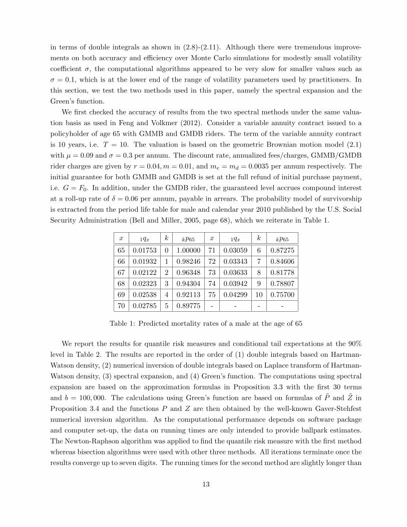
at a roll-up rate of δ = 0.06 per annum, payable in arrears. The probability model of survivorship

is extracted from the period life table for male and calendar year 2010 published by the U.S. Social

Security Administration (Bell and Miller, 2005, page 68), which we reiterate in Table 1.

x 1qx k kp65 x 1qx k kp65

65 0.01753 0 1.00000 71 0.03059 6 0.87275

66 0.01932 1 0.98246 72 0.03343 7 0.84606

67 0.02122 2 0.96348 73 0.03633 8 0.81778

68 0.02323 3 0.94304 74 0.03942 9 0.78807

69 0.02538 4 0.92113 75 0.04299 10 0.75700

70 0.02785 5 0.89775 - - - -

Table 1: Predicted mortality rates of a male at the age of 65

We report the results for quantile risk measures and conditional tail expectations at the 90%

level in Table 2. The results are reported in the order of (1) double integrals based on Hartman-

Watson density, (2) numerical inversion of double integrals based on Laplace transform of Hartman-

Watson density, (3) spectral expansion, and (4) Green’s function. The computations using spectral

expansion are based on the approximation formulas in Proposition 3.3 with the first 30 terms

and b = 100, 000. The calculations using Green’s function are based on formulas of P and Z in

Proposition 3.4 and the functions P and Z are then obtained by the well-known Gaver-Stehfest

numerical inversion algorithm. As the computational performance depends on software package

and computer set-up, the data on running times are only intended to provide ballpark estimates.

The Newton-Raphson algorithm was applied to find the quantile risk measure with the first method

whereas bisection algorithms were used with other three methods. All iterations terminate once the

results converge up to seven digits. The running times for the second method are slightly longer than

13

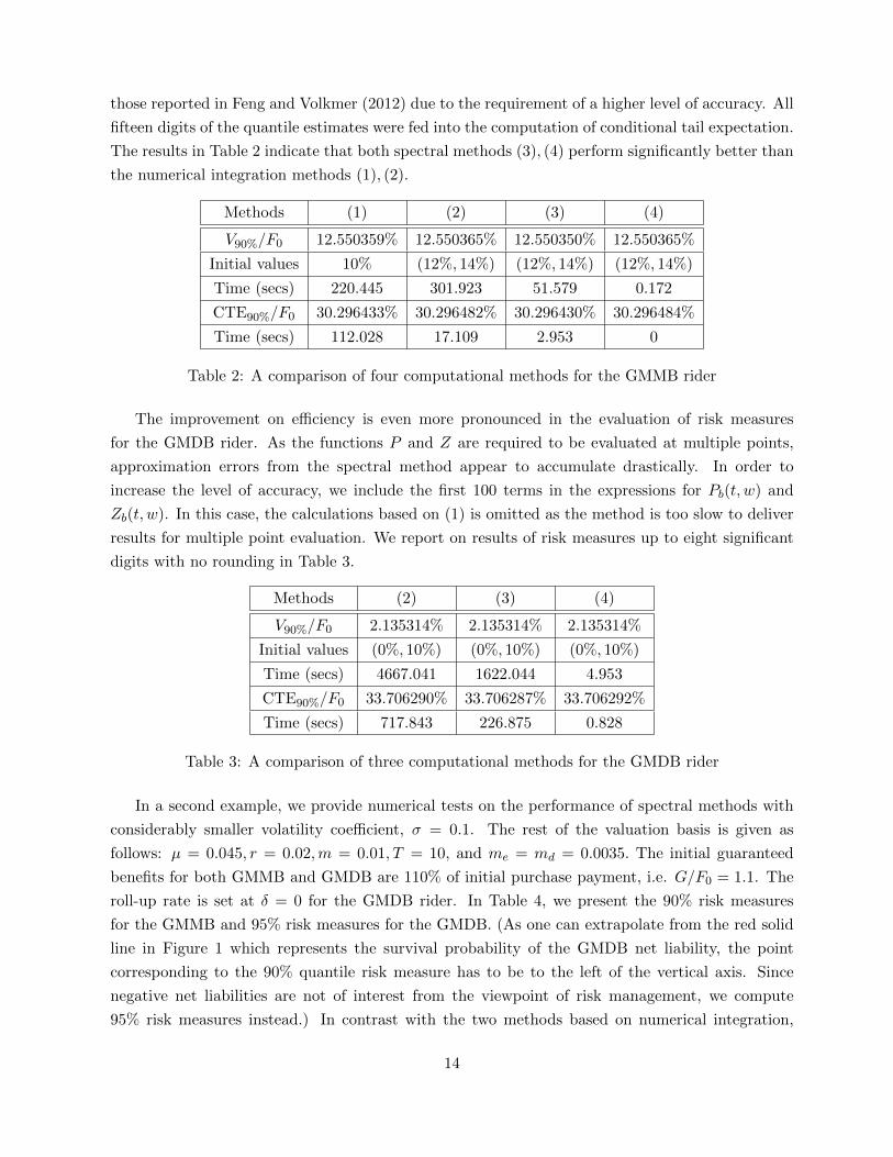
those reported in Feng and Volkmer (2012) due to the requirement of a higher level of accuracy. All

fifteen digits of the quantile estimates were fed into the computation of conditional tail expectation.

The results in Table 2 indicate that both spectral methods (3), (4) perform significantly better than

the numerical integration methods (1), (2).

Methods (1) (2) (3) (4)

V90%/F0 12.550359% 12.550365% 12.550350% 12.550365%

Initial values 10% (12%, 14%) (12%, 14%) (12%, 14%)

Time (secs) 220.445 301.923 51.579 0.172

CTE90%/F0 30.296433% 30.296482% 30.296430% 30.296484%

Time (secs) 112.028 17.109 2.953 0

Table 2: A comparison of four computational methods for the GMMB rider

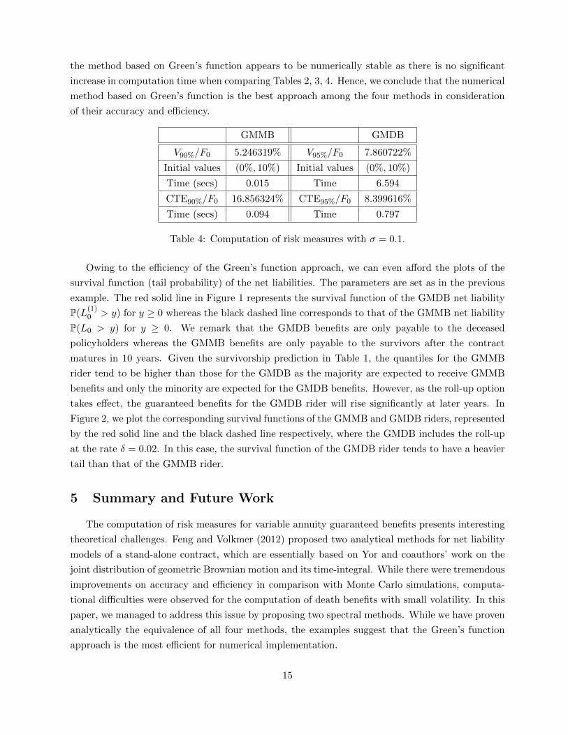
The improvement on efficiency is even more pronounced in the evaluation of risk measures

for the GMDB rider. As the functions P and Z are required to be evaluated at multiple points,

approximation errors from the spectral method appear to accumulate drastically. In order to

increase the level of accuracy, we include the first 100 terms in the expressions for Pb(t, w) and

Zb(t, w). In this case, the calculations based on (1) is omitted as the method is too slow to deliver

results for multiple point evaluation. We report on results of risk measures up to eight significant

digits with no rounding in Table 3.

Methods (2) (3) (4)

V90%/F0 2.135314% 2.135314% 2.135314%

Initial values (0%, 10%) (0%, 10%) (0%, 10%)

Time (secs) 4667.041 1622.044 4.953

CTE90%/F0 33.706290% 33.706287% 33.706292%

Time (secs) 717.843 226.875 0.828

Table 3: A comparison of three computational methods for the GMDB rider

In a second example, we provide numerical tests on the performance of spectral methods with

considerably smaller volatility coefficient, σ = 0.1. The rest of the valuation basis is given as

follows: µ = 0.045, r = 0.02,m = 0.01, T = 10, and me = md = 0.0035. The initial guaranteed

benefits for both GMMB and GMDB are 110% of initial purchase payment, i.e. G/F0 = 1.1. The

roll-up rate is set at δ = 0 for the GMDB rider. In Table 4, we present the 90% risk measures

for the GMMB and 95% risk measures for the GMDB. (As one can extrapolate from the red solid

line in Figure 1 which represents the survival probability of the GMDB net liability, the point

corresponding to the 90% quantile risk measure has to be to the left of the vertical axis. Since

negative net liabilities are not of interest from the viewpoint of risk management, we compute

95% risk measures instead.) In contrast with the two methods based on numerical integration,

14

the method based on Green’s function appears to be numerically stable as there is no significant

increase in computation time when comparing Tables 2, 3, 4. Hence, we conclude that the numerical

method based on Green’s function is the best approach among the four methods in consideration

of their accuracy and efficiency.

GMMB GMDB

V90%/F0 5.246319% V95%/F0 7.860722%

Initial values (0%, 10%) Initial values (0%, 10%)

Time (secs) 0.015 Time 6.594

CTE90%/F0 16.856324% CTE95%/F0 8.399616%

Time (secs) 0.094 Time 0.797

Table 4: Computation of risk measures with σ = 0.1.

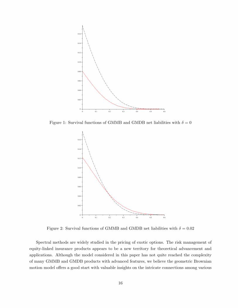
Owing to the efficiency of the Green’s function approach, we can even afford the plots of the

survival function (tail probability) of the net liabilities. The parameters are set as in the previous

example. The red solid line in Figure 1 represents the survival function of the GMDB net liability

P(L(1)0 > y) for y ≥ 0 whereas the black dashed line corresponds to that of the GMMB net liability

P(L0 > y) for y ≥ 0. We remark that the GMDB benefits are only payable to the deceased

policyholders whereas the GMMB benefits are only payable to the survivors after the contract

matures in 10 years. Given the survivorship prediction in Table 1, the quantiles for the GMMB

rider tend to be higher than those for the GMDB as the majority are expected to receive GMMB

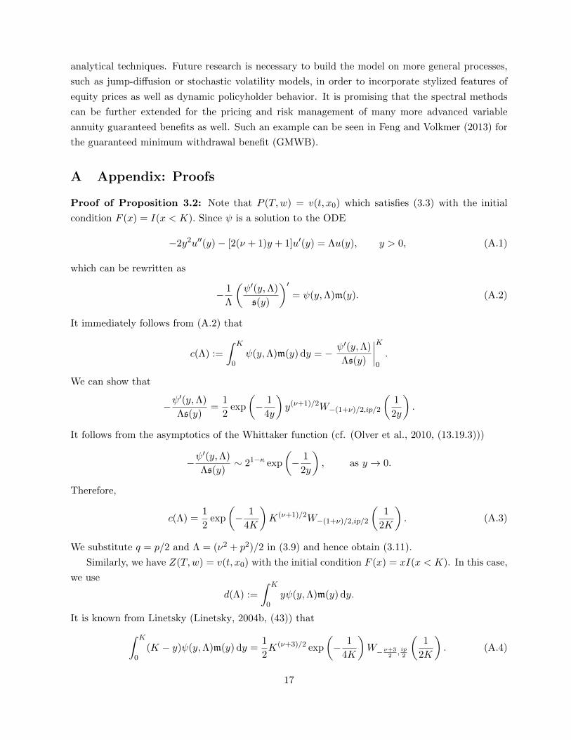
benefits and only the minority are expected for the GMDB benefits. However, as the roll-up option

takes effect, the guaranteed benefits for the GMDB rider will rise significantly at later years. In

Figure 2, we plot the corresponding survival functions of the GMMB and GMDB riders, represented

by the red solid line and the black dashed line respectively, where the GMDB includes the roll-up

at the rate δ = 0.02. In this case, the survival function of the GMDB rider tends to have a heavier

tail than that of the GMMB rider.

5 Summary and Future Work

The computation of risk measures for variable annuity guaranteed benefits presents interesting

theoretical challenges. Feng and Volkmer (2012) proposed two analytical methods for net liability

models of a stand-alone contract, which are essentially based on Yor and coauthors’ work on the

joint distribution of geometric Brownian motion and its time-integral. While there were tremendous

improvements on accuracy and efficiency in comparison with Monte Carlo simulations, computa-

tional difficulties were observed for the computation of death benefits with small volatility. In this

paper, we managed to address this issue by proposing two spectral methods. While we have proven

analytically the equivalence of all four methods, the examples suggest that the Green’s function

approach is the most efficient for numerical implementation.

15

Figure 1: Survival functions of GMMB and GMDB net liabilities with δ = 0

Figure 2: Survival functions of GMMB and GMDB net liabilities with δ = 0.02

Spectral methods are widely studied in the pricing of exotic options. The risk management of

equity-linked insurance products appears to be a new territory for theoretical advancement and

applications. Although the model considered in this paper has not quite reached the complexity

of many GMMB and GMDB products with advanced features, we believe the geometric Brownian

motion model offers a good start with valuable insights on the intricate connections among various

16

analytical techniques. Future research is necessary to build the model on more general processes,

such as jump-diffusion or stochastic volatility models, in order to incorporate stylized features of

equity prices as well as dynamic policyholder behavior. It is promising that the spectral methods

can be further extended for the pricing and risk management of many more advanced variable

annuity guaranteed benefits as well. Such an example can be seen in Feng and Volkmer (2013) for

the guaranteed minimum withdrawal benefit (GMWB).

A Appendix: Proofs

Proof of Proposition 3.2: Note that P (T,w) = v(t, x0) which satisfies (3.3) with the initial

condition F (x) = I(x < K). Since ψ is a solution to the ODE

−2y2u′′(y)− [2(ν + 1)y + 1]u′(y) = Λu(y), y > 0, (A.1)

which can be rewritten as

− 1

Λ

(ψ′(y,Λ)

s(y)

)′= ψ(y,Λ)m(y). (A.2)

It immediately follows from (A.2) that

c(Λ) :=

∫ K

0ψ(y,Λ)m(y) dy = − ψ′(y,Λ)

Λs(y)

∣∣∣∣K0

.

We can show that

−ψ′(y,Λ)

Λs(y)=

1

2exp

(− 1

4y

)y(ν+1)/2W−(1+ν)/2,ip/2

(1

2y

).

It follows from the asymptotics of the Whittaker function (cf. (Olver et al., 2010, (13.19.3)))

−ψ′(y,Λ)

Λs(y)∼ 21−κ exp

(− 1

2y

), as y → 0.

Therefore,

c(Λ) =1

2exp

(− 1

4K

)K(ν+1)/2W−(1+ν)/2,ip/2

(1

2K

). (A.3)

We substitute q = p/2 and Λ = (ν2 + p2)/2 in (3.9) and hence obtain (3.11).

Similarly, we have Z(T,w) = v(t, x0) with the initial condition F (x) = xI(x < K). In this case,

we use

d(Λ) :=

∫ K

0yψ(y,Λ)m(y) dy.

It is known from Linetsky (Linetsky, 2004b, (43)) that∫ K

0(K − y)ψ(y,Λ)m(y) dy =

1

2K(ν+3)/2 exp

(− 1

4K

)W− ν+3

2, ip2

(1

2K

). (A.4)

17

In view of (A.3) and (A.4) we obtain

d(Λ) =1

2K(ν+3)/2 exp

(− 1

4K

)[W− ν+1

2, ip2

(1

2K

)−W− ν+3

2, ip2

(1

2K

)]. (A.5)

Thus we arrive at (3.12) using Λ = (ν2 + p2)/2 and (A.5) in (3.10).

Proof of Proposition 3.3: We approximate P (T,w) by

Pb(T,w) := Px0 [Xt < K, t < Tb] ,

where Tb := inft ≥ 0 : Xt = b and b K. We denote by pb(t;x, y) the transition probability

density with respect to the speed measure of the diffusion process (3.1) started at x ∈ [0, b) and

killed at b. According to Linetsky (2004b), the transition probability density pb(t;x, y) is given by

pb(t;x, y) =∞∑n=1

e−Λntψ(x,Λn)ψ(y,Λn)

‖ ψ(·,Λn) ‖2, (A.6)

where Λn, ψn∞n=1 are eigenvalues and eigenfunctions of the Sturm-Liouville problem

− Gu(x)− Λu(x) = 0, x ∈ (0, b), (A.7)

with the boundary conditions at 0 and b given by

limx↓0

u′(x)

s(x)= 0 (entrance boundary), (A.8)

u(b) = 0 (absorption boundary). (A.9)

Equation (A.7) can also be written as

− 1

m(x)

(u′(x)

s(x)

)′= Λu(x), x ∈ (0, b). (A.10)

The eigenfunctions ψn form an orthonormal basis in L2(m, [0, b]) with the inner product (f, g) =∫ b0 f(x)g(x)m(x)dx and the norm ‖ f ‖2= (f, f). For t > 0, the spectral representation (A.6)

converges uniformly in x, y on [0, b]× [0, b].

One can show that the solution to (A.7) satisfying the boundary condition (A.8) is given by

ψ(x,Λ) = x(1−ν)/2 exp 1

4xWκ,µ

(1

2x

).

Since the eigenfunction ψ must also satisfy the boundary condition (A.9), we can determine the

eigenvalues by finding the zeros of ψ(b,Λ). Let 0 < p1 < p2 < · · · < pn < · · · be the positive

solutions to (3.15). The eigenvalues are Λn = (ν2 + p2n)/2, n = 1, 2, · · · . The eigenfunctions are

given by

ψ(x,Λn) = x(1−ν)/2 exp 1

4xW(1−ν)/2,(ipn)/2

(1

2x

), n = 1, 2, · · · . (A.11)

18

The norms of these eigenfunctions are given in (Linetsky, 2004b, (33)) by

1

‖ ψ(·,Λn) ‖2=

2pnΓ((ν + ipn)/2)

Γ(1 + ipn)ξnM(1−ν)/2,(ipn)/2

(1

2b

), n = 1, 2, · · · . (A.12)

Therefore, the approximation of P (T,w) is given by

Pb(T,w) =

∫ K

0pb(t;x0, y)m(y) dy =

∞∑n=1

e−Λnt ψ(x0,Λn)

‖ ψ(·,Λn) ‖2

∫ K

0ψ(y,Λn)m(y) dy. (A.13)

Hence,

Pb(T, Vα)

=∞∑n=1

2cne−(ν2+p2n)t/2x

1−ν2

0 e1

4x0pnΓ(ν+ipn

2 )

Γ(1 + ipn)ξnM(1−ν)/2,ipn/2

(1

2b

)W(1−ν)/2,ipn/2

(1

2x0

),

where

cn :=

∫ K

0ψ(y,Λn)m(y) dy =

1

2e−1/(4K)K(ν+1)/2W−(1+ν)/2,ipn/2

(1

2K

),

using the same arguments as for (A.3). Thus we arrive at the solution (3.13).

Similarly, we can approximate Z(T,w) by

Zb(T,w) :=1

x0Ex0

[XtIXt<K,t<Tb

]=

1

x0

∫ K

0ypb(t;x0, y)m(y) dy.

Hence,

Zb(T, Vα) =1

x0

∞∑n=1

e−Λnt ψ(x0,Λn)

‖ ψ(·,Λn) ‖2dn,

where as proven in (A.5)

dn =1

2K(ν+3)/2e−1/(4K)

[W−(ν+1)/2,ipn/2

(1

2K

)−W−(ν+3)/2,ipn/2

(1

2K

)].

Therefore, we obtain (3.14) after inserting the expression for dn.

Proof of Proposition 3.4: Let

fκ(y) = y−κ exp

− 1

4y

Mκ,η

(1

2y

), gκ(y) = y−κ exp

− 1

4y

Wκ,η

(1

2y

).

It is easy to show that

f ′κ(y) = −(12 + η + κ)fκ+1(y), g′κ(y) = gκ+1(y),

limy→0+

fκ(y) = 2κΓ(1 + 2η)

Γ(η − κ+ 12), lim

y→0+gκ(y) = 0.

19

Suppose w ≤ 1 so that K = wx0 ≤ x0. In light of (3.19), (3.20), we obtain

P (s, w) =8

σ2

Γ(η − κ+ 12)

Γ(1 + 2η)ψ2

(x0,−

4s

σ2

)∫ K

0ψ1

(y,−4s

σ2

)m(y) dy

=4

σ2

Γ(η − κ+ 12)

Γ(1 + 2η)ψ2

(x0,−

4s

σ2

)∫ K

0gκ(y) dy (A.14)

=4

σ2

Γ(η − κ+ 12)

Γ(1 + 2η)ψ2

(x0,−

4s

σ2

)gκ−1(K).

Inserting the expressions for ψ2 and g we obtain (3.22).

Similarly, we have

Z(s, w) =8

x0σ2

Γ(η − κ+ 12)

Γ(1 + 2η)ψ2

(x0,−

4s

σ2

)∫ K

0yψ1

(y,−4s

σ2

)m(y) dy

=4

x0σ2

Γ(η − κ+ 12)

Γ(1 + 2η)ψ2

(x0,−

4s

σ2

)∫ K

0ygκ(y) dy (A.15)

=4

x0σ2

Γ(η − κ+ 12)

Γ(1 + 2η)ψ2

(x0,−

4s

σ2

)[Kgκ−1(K)− gκ−2(K)]

which leads to (3.23).

Now suppose w > 1 so that K > x0. Splitting the expression for P into two parts, we obtain

σ2

4P (s, w) =

∫ x0

0G(x, y,−4s

σ2)m(y) dy +

∫ K

x0

G(x, y,−4s

σ2)m(y) dy

=Γ(η − κ+ 1

2)

Γ(1 + 2η)x0

[Mκ,η

(1

2x0

)Wκ−1,η

(1

2x0

)+

1

η + κ− 12

Wκ,η

(1

2x0

)Mκ−1,η

(1

2x0

)

− 1

η + κ− 12

w1−κ exp

1

4x0(1− 1

w)

Wκ,η

(1

2x0

)Mκ−1,η

(1

2x0w

)]. (A.16)

We simplify this formula using the following observation. If κ > 12 then F (x) = 1 is in L2(m, (0,∞)).

Obviously, v(Λ, x) = − 1Λ is the solution of (3.17) in L2(m, (0,∞)). Therefore,

− 1

Λ=

∫ ∞0

G(x, y,Λ)m(y) dy for x > 0. (A.17)

Comparing with (A.16) as w →∞, we find (setting z = 12x0

and using −Λ2 = (η−κ+ 1

2)(η+κ− 12))

Mκ,η(z)Wκ−1,η(z) +1

η + κ− 12

Mκ−1,η(z)Wκ,η(z) =zΓ(1 + 2η)

(η + κ− 12)Γ(η − κ+ 3

2). (A.18)

Identity (A.18) holds for all values of κ, η (dropping the assumption κ > 12) as we see by inserting

the differentiation formulas

M ′κ,η(z) =

(1

2− κ

z

)Mκ,η(z) +

1

z(η + κ+ 1

2)Mκ+1,η(z),

W ′κ,η(z) =

(1

2− κ

z

)Wκ,η(z)−

1

zWκ+1,η(z).

20

into the Wronskian of Whittaker function,

M ′κ,µ(z)Wκ,µ(z)−Mκ,µ(z)W ′κ,µ(z) =Γ(1 + 2µ)

Γ(1/2 + µ− κ).

Therefore, (A.16) leads to (3.24).

Similarly, we obtain

σ2

4x0Z(s, w) =

Γ(η − κ+ 12)

Γ(1 + 2η)

[Mκ,η

(1

2x0

)(Wκ−1,η

(1

2x0

)−Wκ−2,η

(1

2x0

))(A.19)

+1

η + κ− 12

Wκ,η

(1

2x0

)(Mκ−1,η

(1

2x0

)+

1

η + κ− 32

Mκ−2,η

(1

2x0)

))

− w2−κ

η + κ− 12

exp

1

4x0(1− 1

w)

Wκ,η

(1

2x0

)Mκ−2,η

(1

2x0w

)η + κ− 3

2

+Mκ−1,η

(1

2x0w

)].We may simplify this formula using the following observation. If κ > 3/2 then F (x) = x is in

L2(m, (0,∞)). Then the corresponding solution of (3.17) is

v(Λ, x) =1− Λx

Λ(Λ + 2(ν + 1)).

Therefore, we have

1− Λx

Λ(Λ + 2(ν + 1))=

∫ ∞0

G(x, y,Λ)ym(y) dy for x > 0. (A.20)

By comparing with (A.19) as w →∞, we obtain (with z = 12x0

)

Mκ,η(z) (Wκ−1,η(z)−Wκ−2,η(z)) +Wκ,η(z)

η + κ− 12

(Mκ−1,η(z) +

Mκ−2,η(z)

η + κ− 32

)

=Γ(1 + 2η)

Γ(η − κ+ 32)

z

η + κ− 12

(1− 2κ− 2− z

(η − κ+ 32)(η + κ− 3

2)

). (A.21)

This identity holds for all κ, η (dropping the assumption κ > 3/2) as we can see from recursion

formulas (Olver et al., 2010, 13.15.1, 13.15.11) for Whittaker functions in combination with (A.18).

Now (A.19) and (A.21) lead to (3.25).

Proof of Remark 3.2: We note that

P (T,w)− Pb(T,w) =Px0(Xt < K)− Px0(Xt < K, t < Tb) = Px0(Xt < K,Tb ≤ t)

≤Px0(Tb ≤ t) = Px0(

max0≤s≤t

Xt ≥ b).

Since ν > 0 by assumption and X is a submartingale, it follows by Doob’s maximal inequality that

P (T,w)− Pb(T,w) ≤ 1

bEx0 [Xt] =

x0

be2(ν+1)t +

1

2(ν + 1)b(e2(ν+1)t − 1).

21

Similarly, we note that

Z(T,w)− Zb(T,w) =1

x0Ex0 [XtI(Xt < K)]− 1

x0Ex0 [XtI(Xt < K, t < Tb)]

≤ 1

x0Ex0 [XtI(Tb ≤ t,Xt < K)] ≤ 1

x0KPx0

(max0≤s≤t

Xt ≥ b).

Proof of Remark 3.3: Here we reiterate the first formula for P

P1(s, w) =4

σ2

∫ √w0

∫ (w−ρ2)x0

0

ρν−1

uexp

− 1

2u(1 + ρ2)

I2η

(ρu

)dudρ. (A.22)

According to (A.14), the second formula for P is equivalent to

P2(s, w) =4

σ2

Γ(η − κ+ 12)

Γ(1 + 2η)xκ0 exp

1

4x0

Mκ,η

(1

2x0

)∫ x0w

0y−κ exp

− 1

4y

Wκ,η

(1

2y

)dy.

In (A.22) we make the substitution

u =2y

cosh v + 1, ρ =

√y

x0

cosh v − 1

sinh v=

√y

x0tanh

v

2. (A.23)

The new variables of integration are v and y. The corresponding limits for these variables are

0 < v <∞ and 0 < y < wx0. The Jacobian is√y

x0

1

cosh v + 1.

Note that1

2u(1 + ρ2) =

1

4x0(cosh v − 1) +

1

4y(cosh v + 1),

ρ

u=

sinh v

2√x0y

.

After performing the substitution and simplifying we obtain

σ2

4P1(s, w) =

1

2

∫ x0w

0xκ− 1

20 e

14x0 y−κ−

12 e− 1

4y

∫ ∞0

exp(−(

14x0

+ 14y

)cosh v

)coth2κ v

2I2η(sinh v2√x0y

) dv dy.

(A.24)

We now use formula (56) in (Buchholz, 1953, page 86):

Mκ,η(a1)Wκ,η(a2) =√a1a2

Γ(1 + 2η)

Γ(η − κ+ 12)

∫ ∞0

exp(−a1+a22 cosh v) coth2κ v

2I2η(√a1a2 sinh v) dv

(A.25)

provided that 0 < a1 < a2. We apply (A.25) with a1 = 1/(2x0) , a2 = 1/(2y) in (A.24), and we

obtain P1 = P2.

Using the transformation (A.23), we also verify that (3.23) and (2.11) agree. We note that the

identity

tanh2 v

2= 1− 2

cosh v + 1

implies ρ2x0 = y − u and thusρν+1

u+ρν−1

x0=ρν−1

u

y

x0.

Then we argue as above to show that (2.11) transforms to (A.15).

22

References

Bacinello, A. R., Millossovich, P., Olivieri, A., and Pitacco, E. (2011). Variable annuities: a unifying

valuation approach. Insurance Math. Econom., 49(3):285–297.

Bauer, D., Kling, A., and Russ, J. (2008). A universal pricing framework for guaranteed minimum

benefits in variable annuities. Astin Bull., 38(2):621–651.

Bell, F. and Miller, M. (2005). Life Tables for the United States Social Security Area. Social

Security Administration Publications No. 11-11536.

Boyarchenko, N. and Levendorskiı, S. (2007). The eigenfunction expansion method in multi-factor

quadratic term structure models. Math. Finance, 17(4):503–539.

Buchholz, H. (1953). Die konfluente hypergeometrische Funktion mit besonderer Berucksichtigung

ihrer Anwendungen. Ergebnisse der angewandten Mathematik. Bd. 2. Springer-Verlag, Berlin.

Chen, Z. and Forsyth, P. A. (2008). A numerical scheme for the impulse control formulation for

pricing variable annuities with a guaranteed minimum withdrawal benefit (GMWB). Numer.

Math., 109(4):535–569.

Dai, M., Kwok, Y. K., and Zong, J. (2008). Guaranteed minimum withdrawal benefit in variable

annuities. Math. Finance, 18(4):595–611.

Davydov, D. and Linetsky, V. (2003). Pricing options on scalar diffusions: an eigenfunction expan-

sion approach. Oper. Res., 51(2):185–209.

Donati-Martin, C., Ghomrasni, R., and Yor, M. (2001). On certain Markov processes attached to

exponential functionals of Brownian motion; application to Asian options. Rev. Mat. Iberoamer-

icana, 17(1):179–193.

Farr, I., Mueller, H., Scanlon, M., and Stronkhorst, S. (2008). Economic Capital for Life Insurance

Companies. SOA Monograph.

Feng, R. (2014). A comparative study of risk measures for guaranteed minimum maturity benefits

by a PDE method. North American Actuarial Journal, 18 (4), to appear.

Feng, R. and Volkmer, H. (2012). Analytical calculation of risk measures for variable annuity

guaranteed benefits. Insurance Math. Econom., 51(3):636–648.

Feng, R. and Volkmer, H. (2013). An identity of hitting times and its application to the valuation

of guaranteed minimum withdrawal benefit. Preprint.

Fouque, J.-P., Jaimungal, S., and Lorig, M. J. (2011). Spectral decomposition of option prices in

fast mean-reverting stochastic volatility models. SIAM J. Financial Math., 2:665–691.

23

Gorski, L. M. and Brown, R. A. (2005). Recommended approach for setting regulatory risk-based

capital requirements for variable annuities and similar products. Technical report, American

Academy of Actuaries Life Capital Adequacy Subcommittee, Boston.

Jeanblanc, M., Yor, M., and Chesney, M. (2009). Mathematical methods for financial markets.

Springer Finance. Springer-Verlag London Ltd., London.

Karatzas, I. and Shreve, S. E. (1991). Brownian motion and stochastic calculus, volume 113 of

Graduate Texts in Mathematics. Springer-Verlag, New York, second edition.

Kyprianou, A. E. (2006). Introductory lectures on fluctuations of Levy processes with applications.

Universitext. Springer-Verlag, Berlin.

Lewis, A. L. (1998). Applications of eigenfunction expansions in continuous-time finance. Math.

Finance, 8(4):349–383.

Linetsky, V. (2004a). The spectral decomposition of the option value. Int. J. Theor. Appl. Finance,

7(3):337–384.

Linetsky, V. (2004b). Spectral expansions for Asian (average price) options. Oper. Res., 52(6):856–

867.

Milevsky, M. A. and Salisbury, T. S. (2006). Financial valuation of guaranteed minimum withdrawal

benefits. Insurance Math. Econom., 38(1):21–38.

Øksendal, B. (2003). Stochastic differential equations. Universitext. Springer-Verlag, Berlin, sixth

edition. An introduction with applications.

Olver, F. W. J., Lozier, D. W., Boisvert, R. F., and Clark, C. W., editors (2010). NIST handbook

of mathematical functions. U.S. Department of Commerce National Institute of Standards and

Technology, Washington, DC.

Piscopo, G. and Haberman, S. (2011). The valuation of guaranteed lifelong withdrawal benefit

options in variable annuity contracts and the impact of mortality risk. N. Am. Actuar. J.,

15(1):59–76.

Yor, M. (1992). On some exponential functionals of Brownian motion. Adv. in Appl. Probab.,

24(3):509–531.

24