SPECTRAL METHODS FOR VOLATILITY DERIVATIVES - Munich

MPRAMunich Personal RePEc Archive

SPECTRAL METHODS FORVOLATILITY DERIVATIVES

Claudio Albanese and Aleksandar Mijatovic

Independent Consultant

1. March 2006

Online at http://mpra.ub.uni-muenchen.de/5244/MPRA Paper No. 5244, posted 10. October 2007

http://mpra.ub.uni-muenchen.de/

http://mpra.ub.uni-muenchen.de/5244/

SPECTRAL METHODS FOR VOLATILITY DERIVATIVES

CLAUDIO ALBANESE, HARRY LO, AND ALEKSANDAR MIJATOVIC

Abstract. In the first quarter of 2006 Chicago Board Options Exchange (CBOE) introduced,

as one of the listed products, options on its implied volatility index (VIX). This opened thechallenge of developing a pricing framework that can simultaneously handle European options,

forward-starts, options on the realized variance and options on the VIX. In this paper we

propose a new approach to this problem using spectral methods. We define a stochasticvolatility model with jumps and local volatility, which is almost stationary, and calibrate it

to the European options on the S&P 500 for a broad range of strikes and maturities. We thenextend the model, by lifting the corresponding Markov generator, to keep track of relevant

path information, namely the realized variance. The lifted generator is too large a matrix to

be diagonalized numerically. We overcome this difficulty by developing a new semi-analyticalgorithm for block-diagonalization. This method enables us to evaluate numerically the joint

distribution between the underlying stock price and the realized variance which in turn gives

us a way of pricing consistently the European options, general accrued variance payoffs as wellas forward-starts and VIX options.

1. Introduction

In recent years there has been much interest in trading derivative products whose underlyingis a realized variance of some liquid financial instrument (e.g. S&P 500) over the life of thecontract. The most popular payoff functions1 are linear, leading to variance swaps, square root,yielding volatility swaps, and the usual put and call payoffs defining variance swaptions.

It is clear that the plethora of possible derivatives on the realized variance is closely related tothe standard volatility-sensitive instruments like vanilla options, which are also exposed to othermarket risks, and the forward starting options which are almost pure vega bets and are mainlyexposed to the movements of the forward smile. Recently Chicago Board Options Exchange(CBOE) introduced options on the volatility index2 (VIX) which are also important predictorsfor the future behaviour of implied volatility. The main purpose of this paper is to introduce aframework in which all of the above financial instruments (i.e. the derivatives on the realizedvariance as well as the instruments depending on the implied volatility) can be priced and hedgedconsistently and efficiently.

Our central idea is very simple and can be described as follows. We define a dynamics for theunderlying that includes local volatility, stochastic volatility and jumps and can be calibrated tothe implied volatility surface for a wide variety of strikes and maturities (for the case of Europeanoptions on the S&P 500 see figure 1). The underlying process is stationary as can be inferredfrom the fact that the implied forward volatility smile behaves in a consistent way (see figures 7,8, 9 and 10). This is a consequence of the minimal explicit time-dependence in the calibrationof the model.

There are two features of this model that make it possible to obtain the distributions of thefuture behaviour of implied volatility and of the realized variance of the underlying. The firstfeature is the complete numerical solubility of the model. In other words spectral theory providesa simple and efficient algorithm (see subsection 3.5) for obtaining a conditional probabilitydistribution function for the underlying between any given pair of times in the future. Thisproperty is sufficient to determine completely the forward volatility smile and the distribution

1For the precise definition of these products see subsections 2.1 and 2.2.2For a brief description of the these securities see subsection 2.3. For the definition of VIX see (CBOE 2003).

1

2 CLAUDIO ALBANESE, HARRY LO, AND ALEKSANDAR MIJATOVIC

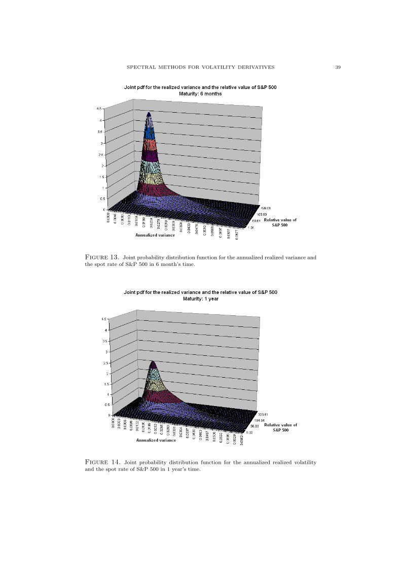
of VIX for any maturity. The second feature of the framework that makes it possible to dealwith the realized variance is the extendability property of Markov generators known as lifting(for details see section 5). This allows us to define a new Markov generator of an extendedprocess which keeps track both of the realized variance and the underlying forward rate. Using ablock-diagonalization algorithm, described in section 6, and the standard methods from spectraltheory we find a joint probability distribution function for the underlying process and its realizedvariance or volatility at any time in the future (for time horizons of 6 months, 1 year and 2 yearssee figures 13, 14 and 15 respectively). This joint pdf is precisely what is needed to price acompletely general payoff which depends on the realized variance and on the underlying.

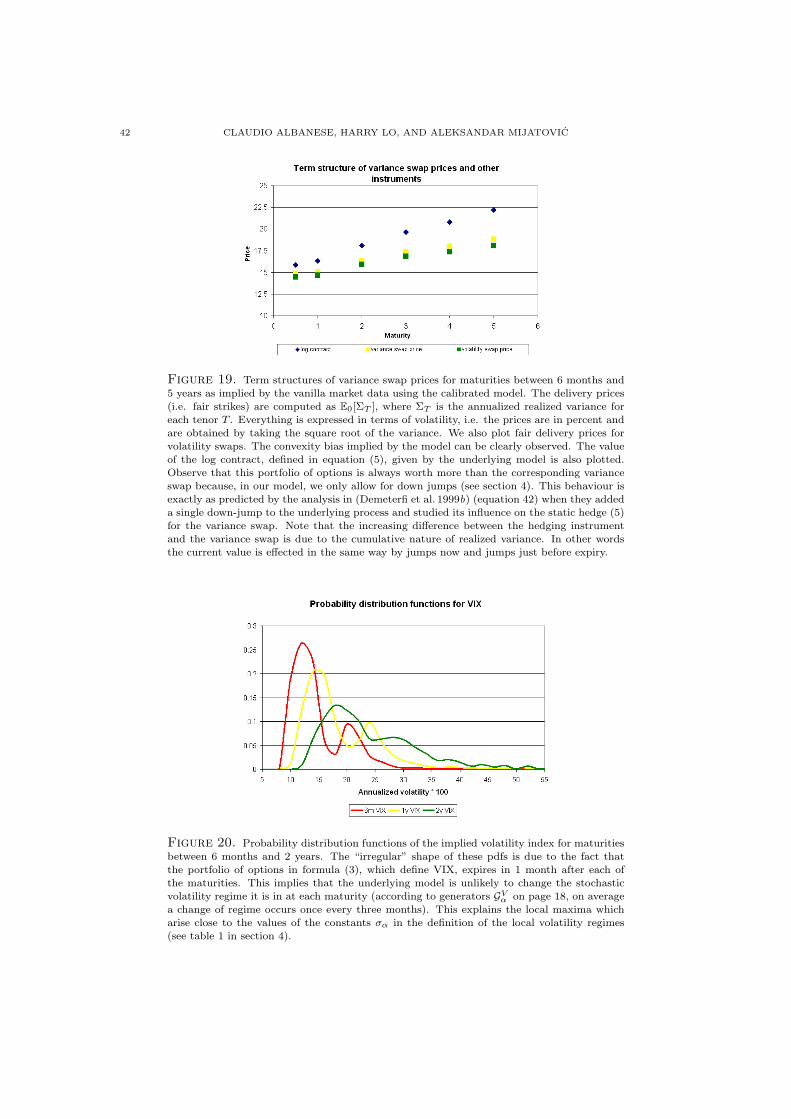
There are two natural and useful consequences of this approach. One is that we do not need tospecify exogenously the process for the variance and then try to find an arbitrage-free dynamicsfor the underlying, but instead imply such a process from the observed vanilla market via themodel for the underlying (a term-structure of the fair values of variance swaps as implied bythe vanilla market data and our model is shown in figure 19). The second consequence is thatthis approach bypasses the use of Monte Carlo techniques and therefore yields sharp and easilycomputable sensitivities to the market parameters. This is because the pricing algorithm yields,as a by-product, all the necessary information for finding the required hedge-ratios.

There is a rapidly growing interest in trading volatility derivatives in financial markets whichis mainly a consequence of the following two factors. On one hand pure volatility instruments areused to hedge implicit vega exposure of the portfolios of market participants, thus bypassing theneed to trade frequently in the vanilla options market, which in itself is advantageous becauseof the relatively large bid-offer spreads prevailing in that market. On the other hand volatilityderivatives are a useful tool for speculating on the future volatility levels and for trading thedifference between realized and implied volatility.

This interest is reflected in the vast amount of literature devoted to volatility products. Theanalysis of the realized variance is intrinsically easier than that of realized volatility because of theadditivity of the former. Under the hypothesis that the underlying price process is continuous therealized variance can be hedged perfectly by a European contract with the logarithmic payoff,first studied in (Neuberger 1994), and a dynamic trading strategy in the underlying. Thisapproach does not require an explicit specification for the instantaneous volatility process of theunderlying and can therefore be used within any stochastic volatility framework. This idea hasbeen developed in (Carr & Madan 1998) and (Demeterfi, Derman, Kamal & Zou 1999a) wherethe static replication strategy for the log contract, using calls and puts, is described. Types ofmark-to-market risk faced by a holder of a variance swap are studied and classified in (Chriss& Morokoff October 1999). A direct delta-hedging approach for the realized variance is givenin (Heston & Nandi November 2000).

A shortcoming of pricing variance swaps without specifying a volatility model (as describedin (Carr & Madan 1998) and (Demeterfi, Derman, Kamal & Zou 1999b)) is that this methodologydoes not yield a natural method for the computation of the sensitivities to market parameters (i.e.Greeks). In (Howison, Rafailidis & Rasmussen 2004) a diffusion model for the volatility processis specified which allowed the authors to use PDE technology to price and hedge variance andvolatility swaps as well as more general payoffs. The obstacle here is that, even if one managesto guess the correct dynamics for the instantaneous volatility, the stochastic volatility modelsare known to have difficulties fitting the observed market skews for both the short dated andthe long dated options at the same time.

The derivatives on the realized volatility can be considered naturally as the derivatives onthe square root of the realized variance. In (Brockhaus & Long 1999) the authors provide avolatility convexity correction which relates the two families of derivatives. A practical difficultywith hedging a volatility swap using variance swaps is that it requires a dynamic position in thelog contract which in turn depends on a strip of vanilla options. Some of these options will bevery far out-of-the-money and therefore trading at large bid-offer spreads which would make there-balancing of the hedge a costly exercise.

SPECTRAL METHODS FOR VOLATILITY DERIVATIVES 3

Another approach, pioneered in (Carr & Lee 2004), develops a robust hedging strategy forvolatility derivatives which is analogous to the one for variance swaps. In other words theauthors find a hedge for a volatility swap using a static position in some European derivativeand a dynamic hedging strategy in the underlying. This method works for continuous processesonly and is based on the observation that, under the continuity hypothesis, there is a simplealgebraic relationship between the Laplace transform of the process and the Laplace transform ofits quadratic variation. There are some technical difficulties in computing the relevant integralsfor general payoffs of realized volatility. This issue has been dealt with in (Friz & Gatheral 2005)where a formula in terms of Bessel functions is given for the European payoff that one needs tohold in order to hedge the corresponding volatility payoff.

In (Windcliff, Forsyth & Vetzal 2006) the authors investigate hedging techniques for thediscretely monitored volatility contracts which are independent of the instantaneous volatilitydynamics. Their main result is that the delta hedge of the volatility derivative can be greatly im-proved by an additional gamma hedge using an at-the-money straddle (or an out-of-the-moneystrangle) which is re-balanced at each volatility observation time. The reason behind choos-ing these particular European payoffs lies in the fact that their risk profile resembles that of avolatility swap. Another model-independent hedging approach for variance swaps is presentedin (Schoutens 2005). The author shows that, in an environment with jumps, one can use deriva-tives on the realized higher order moments of the underlying (i.e. the so called moment swaps)to improve the performance of the log contract as a hedge for the variance swap. This strat-egy provides an improved static hedge, as far as derivatives are concerned, but suffers from thefact that in practice moment swaps of order 3 and above are less liquid than variance swapsthemselves.

Another interesting approach to the pricing of volatility derivatives is based on the obser-vation that the term-structure of variance swaps, an example of which is given in figure 19, ismathematically reminiscent of the term-structure of zero-coupon bonds in interest rate mod-elling. A framework, analogous to the famous HJM, has been proposed in (Buehler 2006). Thestarting point is the specification of the function-valued process for the forward instantaneousvariance which yields an arbitrage-free dynamics for the underlying. This model requires theentire variance swap curve at time zero in order to be calibrated. The correlation between thedriving Brownian motion for the stock and the instantaneous variance is used to introduce theubiquitous skew, but is insufficient to reprice the entire volatility surface that can be observedin the market. Since the driving Markov process for this model is high-dimensional, the pricingis done by Monte Carlo.

This paper is organized as follows. In section 2 we shall describe some of the volatility contractsthat can be priced within our framework. Section 3 defines the model for the underlying forwardrate. In section 4 we discuss the calibration of the model to a wide range of strikes and maturitiesfor options written on the S&P 500. The key idea, that of the lifting of a Markov generator,which allows us to price general derivatives on the realized variance, is introduced in section 5.The numerical algorithm required to make this idea applicable is described in section 6. Section 7explains the pricing methodology for derivatives on the realized variance. In section 8 we carryout some numerical experiments and consistency tests on the calibrated model. Concludingremarks are contained in section 9.

2. Volatility derivatives

In this section we are going to give a brief description of the volatility derivatives discussedin this paper. We start with the simplest case, namely a forward on the realized variance,which defines a variance swap. In subsection 2.2 we define options with payoffs that are generalfunctions of realized variance. Subsection 2.3 concerns derivatives that are dependent on impliedvolatility. In particular we recall the definition of the forward starting options and of the impliedvolatility index.


2.1. Variance swaps. As mentioned above, a variance swap expiring at time T is simply aforward contract on the realized variance ΣT , quoted in annual terms, of the underlying stock(or index) over the time interval [0, T ]. The payoff is therefore of the form

(ΣT −Kvar)N,

where Kvar is the strike and N is the notional of the contract. The fair value of the variance isthe delivery price Kvar which makes the swap have zero value at inception.

At present such contracts are liquidly traded for most major indices. The delivery price isusually quoted in the markets as the square of the realized volatility, i.e. Kvar = K2 where K isa value of realized volatility expressed in percent. The notional N is usually quoted in dollarsper square of the volatility point3.

A key part of the specification of a variance swap contract is how one measures the realizedvariance ΣT . There are a number of ways in which discretely sampled returns of an index (or ofan index future4 Ft) can be calculated and used for defining the realized variance. We will nowdescribe the two most common approaches.

The usual definition of the annualized realized (i.e. accrued) variance of the underlyingprocess Ft in the period [0, T ], using logarithmic returns, is d

n

∑ni=1(log Fti

Fti−1)2, where times ti,

for i = 0, . . . , n, are business days from now t0 = 0 until expiry tn = T . The normalizationconstant d is the number of trading days per year. Another frequently used definition of therealized variance is given by d

n

∑ni=1(

Fti−Fti−1

Fti−1)2. It is a standard fact about continuous square-

integrable martingales that in the limit, as we make partitions of the interval [0, T ] finer andfiner, both sums exhibit the following behaviour5:

〈log F 〉t = limn→∞

n∑i=1

(log

Fti

Fti−1

)2

= limn→∞

n∑i=1

(Fti − Fti−1

Fti−1

)2

.

The convergence here is in probability and the process 〈log F 〉t is the quadratic-variation6 processassociated to log(Ft).

In our framework the underlying process Ft will be a continuous-time Markov chain (seechapter 6 of (Grimmett & Stirzaker 2001) for definitions and basic properties). We define theannualized realized variance ΣT (of Ft over the time interval [0, T ]) to be the limit

ΣT :=1T

limρ(n)→0

n∑i=1

(Fti

− Fti−1

Fti−1

)2

,(1)

where, for every n ∈ N, the set (ti)i=0,...,n is a strictly increasing sequence of times between 0and T and ρ(n) := maxti−ti−1; i = 1, . . . , n is the size of the maximal subinterval given by thesequence (ti)i=0,...,n (cf. definitions (18) in section 5 and (19), (20) in subsection 5.1). It shouldbe noted that the techniques described in sections 5 and 6, which provide numerical solubilityfor our model, can be generalized to the situation where the realized variance is defined as adiscretely sampled sum in (1) but without the limit. We are not going to pursue this line of

3A volatility point is one basis point of volatility, i.e. 0.01 if volatility is quoted in percent. This means that

the quote for the notional value of the variance swap tells us how much the swap owner gains if the realizedvariance increases by 0.0001 = 0.012.

4The reason for considering index futures rather than the index itself is twofold. The futures are used for

hedging options on the index because they are much easier to trade than the whole portfolio of stocks that theindex comprises. Also, it is well-known that futures prices are martingales under the appropriate risk-neutral

measure which depends on the frequency of mark-to-market. If the futures contract marks to market continuously,then the price process Ft is a martingale in the risk-neutral measure induced by the money market account as anumeraire. Otherwise we have to take the rollover strategy, with the same frequency as mark-to-market, as our

numeraire to obtain the martingale measure for Ft.5 Notice also that these equalities hold because the difference of the process log(Ft) and

∫ t0

dFuFu

is of finite

variation, which is a consequence of Ito’s lemma (see theorem 3.3 in (Karatzas & Shreve 1998)).6For a precise definition of a quadratic-variation of continuous square-integrable martingales see chapter 1

of (Karatzas & Shreve 1998).


thought any further, but should notice that the discrete definition of the realized variance wouldrequire the application of the block-diagonalization algorithm (section 6) to the probability kernelbetween any two consecutive observation times ti rather than the application of the algorithmto the Markov generator directly, which is what is done in section 7.

2.2. General payoffs of the realized variance. A volatility swap is a derivative given by thepayoff

(σRT −Kvol)N,

where σRT is the realized volatility over the time interval [0, T ] quoted in annual terms, Kvol is

the annualized volatility strike and N is the notional in dollars per volatility point. The marketconvention for calculating the annualized realized volatility σR

T differs slightly from the usualstatistical measure7 of a standard deviation of any discrete sample and is given by the formula

σRT =

√√√√ d

n

n∑i=1

(Fti

− Fti−1

Fti−1

)2

,

where d is the number of trading days per year and ti are business days from now t0 = 0 untilexpiry tn = T of the contract. For our purposes we shall define realized volatility σR

T , quoted inannual terms, over the time interval [0, T ] as

σRT :=

√ΣT ,

where ΣT is the annualized realized variance defined in (1). It is clear from this definition thatthe payoff of the volatility swap can be view as a non-linear function of the realized variance.

Since volatility swaps are always entered into at equilibrium, an important issue is the determi-nation of the fair strike Kvol for any given maturity T . As discussed in section 1, a term structureof such strikes must be part of the market data that some models require (e.g. (Buehler 2006))in order to be calibrated. In our case the strikes Kvol, for any maturity, are implied by themodel which uses as its calibration data the market implied vanilla surface. The value of Kvol

for a given maturity T is then given by the expectation E0[√

ΣT ], which can easily be obtainedas soon as we have the probability distribution function for ΣT .

The same reasoning applies to variance swaps. The fair strike Kvar for the variance swapof maturity T can, within our framework, be obtained by taking the expectation E0[ΣT ]. Ittherefore follows from the concavity of the square root function and Jensen’s inequality8 thatthe following relationship holds between the fair strikes of the variance and volatility swaps

Kvol <√

Kvar,

for any maturity T . This inequality is always satisfied by the market quoted prices for varianceand volatility swaps and is there to account for the fact that variance is a convex function ofvolatility. Put differently, this is just a convexity effect, similar to the one observed for ordinarycall options, related to the magnitude of volatility of volatility. The larger the “vol of vol” is, thegreater the convexity effect becomes. This phenomenon can be observed clearly in the marketswith a very steep skew for implied volatilities. If one wanted to estimate its size in general, itwould be necessary to make assumptions about both the level and volatility of the future realizedvolatility. Within our model this can be achieved directly by comparing the values of the twoexpectations (see figure (19) for this comparison based on the market implied vanilla surface forthe S&P 500).

7Given a sample of n values X1, . . . , Xn with the mean µ = 1n

∑ni=1 Xi, the unbiased statistical estimation

of the standard deviation is given by √√√√ 1

n− 1

n∑i=1

(Xi − µ)2.

8For any convex function φ : R → R and any random variable X : Ω → R with a finite first moment Jensen’sinequality states that φ(E[X]) ≤ E[φ(X)].


There are other variance payoffs which are of practical interest and can be priced and hedgedwithin our framework. Examples are volatility and variance swaptions whose payoffs are (

√ΣT −

Kvol)+ and (ΣT − Kvar)+ respectively, where as usual (x)+ equals max(x, 0) for any x ∈ R.Capped volatility swaps are also traded in the markets. Their payoff function is of the form(min(

√ΣT , σm)−Kvol), where σm denotes the maximum allowed realized variance. It is clear that

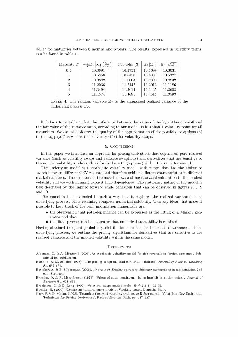
all such contracts can be priced easily within our framework by integrating any of these payoffsagainst the probability distribution function (see figure 11 for maturities above 6 months) of theannualized realized variance ΣT and then multiplying the expectation with the correspondingdiscount factor.

It should be noted that there exist even more exotic products, like corridor variance swaps(see (Carr & Lewis February 2004)), whose payoffs depend on the variance that accrues only ifthe underlying is in a predefined range. Such products cannot be priced directly in the existingframework. A minor modification of the model would be required to deal with this class ofderivatives. However we will not pursue this avenue any further.

2.3. Forward staring options and the volatility index. Let T ′ and T be a pair of maturitiessuch that T ′ < T . A forward staring option (or a forward-start) is a vanilla option with expiry Tand the strike,set at time T ′, which is equal to αST ′ . The quantity St is the underlying financialinstrument the option is written on (usually a stock or an index). More formally the value of aforward-start at time T (i.e. its payoff) is given by

VFS(T ) = (ST − αST ′)+ ,(2)

where the constant α is specified at the inception of the contract and is know as the forwardstrike. It is clear from the definition of the forward-start that its value at time T ′ equals thevalue of a plain vanilla call option

VFS(T ′) = VC(ST ′ , T − T ′, αST ′)

that expires in T − T ′ years and whose strike equals αST ′ . Notice that at time T ′ the constantα can be characterized as the ratio9 between the spot price ST ′ and the strike of the call optioninto which the forward-start is transformed. In the classical Black-Scholes framework, we havean explicit formula, denoted by BS(ST ′ , T − T ′, αST ′ , r′, σ′), for the value of this call option(see (Black & Scholes 1973)). This formula depends linearly on the spot level ST ′ if the ratio ofthe spot and the strike (i.e. the “moneyness”) is known. In other words, assuming we are in theBlack-Scholes world with a deterministic term-structure of volatility and interest rates and zerodividends, we can express the value of the forward-start at time T ′ as

VFS(T ′) = ST ′BS(1, T − T ′, α, r′, σ′),

where σ′ is the forward volatility rate10 and r′ is the forward interest rate between T ′ and T .The following key observations about the Black-Scholes value and sensitivities of the forwardstarting option are now clear:

• the value equals VFS(0) = S0BS(1, T − T ′, α, r′, σ′) and the delta (i.e. ∂∂S0

VFS(0)) issimply BS(1, T − T ′, α, r′, σ′),

• the forward starting option is gamma neutral11 (i.e. ∂2

∂S20VFS(0) = 0) and

• the contract has non-zero vega (i.e. ∂∂σ′VFS(0) > 0).

We are interested in the Black-Scholes pricing formula for the forward-starts because we needto use it when expressing the forward volatility smile of our model. The values of forwardvolatility σ′, implied by the equation VFS(0) = S0BS(1, T −T ′, α, r′, σ′), are plotted in figures 7,

9This ratio is sometimes referred to as the “moneyness” of the option.10Assuming that the term-structure of volatility is parametrized by σ(t), the forward volatility rate σ′ is given

by σ′2 = 1T−T ′

∫ TT ′ σ(t)2dt.

11It should be noted that, in the presence of stochastic volatility, the gamma of a forward starting option is no

longer necessarily zero. However in a realistic model it should not be too large because it reflects the dependenceof volatility on very small moves of the underlying, the effect of which should be negligible.


8, 9 and 10 for a wide range of values of the forward strike α and a variety of time horizonsT ′, T . In other words, we first calculate the value VFS(0) of the forward-start and then invertthe Black-Scholes pricing formula to obtain the implied forward volatility σ′.

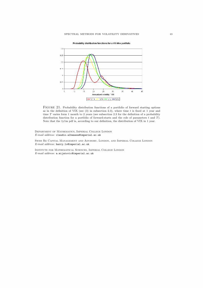
We shall now give a brief description of the implied volatility index (VIX) and then move onto discuss the future probability distribution of VIX, which, as will be seen, is directly relatedto forward starting options.

VIX was originally introduced in 1993 by Chicago Board Options Exchange (CBOE) as anindex reflecting the 1 month implied volatility of the at-the-money put and call options on S&P100. To facilitate trading in VIX, in 2003 CBOE introduced a new calculation, using a fullrange of strikes for out-of-the-money options, to define the value of VIX. At the same time theunderlying financial instrument on which the options are written was changed to S&P 500 (fora detailed description of these changes and their ramifications see (CBOE 2003)). The newformula is

σ2VIX =

2T

∑i

∆Ki

K2i

erT Q(Ki)−1T

(F

K0− 1

)2

,(3)

where the index itself is given by VIX = 100σVIX. The sequence Ki consists of all the ex-change quoted strikes and the quantities Q(Ki) are the corresponding values of out-of-the-moneyput/call options expiring at maturity T , where T equals 1 month12. The quantity F in formula (3)is the forward value of the S&P 500 index derived from option prices13 and the at-the-moneystrike K0 is defined as the largest strike below F . Note also that it is precisely at K0 that thesymbol Q(K) in (3) changes from put to call options.

The reason why formula (3) allows easier trading of volatility follows from the simple obser-vation that σ2

VIX is essentially the value of a European derivative, expiring at time T , with thelogarithmic payoff given in (4). This is a consequence of the well-known decomposition of anytwice differentiable payoff described in (Breeden & Litzenberger 1978), (Carr & Madan 1998),(Demeterfi et al. 1999b) and other sources:

− log(

ST

F

)= −ST − F

F+

∫ F

0

1K2

(K − ST )+dK +∫ ∞

F

1K2

(ST −K)+dK.(4)

This formula holds for any value of F , but expressions simplify if we assume that F equals theforward of the index St at time T (i.e. F = E[ST ]). By taking the expectation with respect tothe risk-neutral measure we get the following expression for the forward price of the log payoff:

− E[log

(ST

F

)]=

∫ F

0

1K2

erT P (K)dK +∫ ∞

F

1K2

erT C(K)dK,(5)

where C(K) = e−rT E[(ST − K)+] (resp. P (K) = e−rT E[(K − ST )+]) is the price of a call(resp. put) option struck at K. It is shown in (Demeterfi et al. 1999b) that the portfolio ofvanilla options given by (5) can be used to hedge perfectly a variance swap if there are no jumpsin the underlying market. From our point of view the expression (5) is interesting because asimple calculation shows that definition (3) is a possible discretization of it. By defining its ownversion of the approximation to the logarithm, CBOE has created a volatility index which canbe replicated by trading a relatively simple European payoff. This feature greatly simplifies thetrading of VIX.

Since the implied volatility index is defined by a portfolio of puts and calls in (3), it is clearthat the random nature of the value of VIX at time t will be determined by the value of the

12The actual CBOE definition of VIX uses two maturities, rather than one, and the two corresponding strips

of options. The value of σ2VIX is then defined to be a convex combination of the two values given by the formula

in (3). Details of this construction can be found in (CBOE 2003). We are going to neglect this technical pointbecause its use is mainly to circumvent certain market irregularities when dealing with options with short timeto expiry and does not add complexity to the modelling side of the problem.

13See page 3 in (CBOE 2003) for the precise definition.


corresponding portfolio of forward starting options. The probability distribution function forthe behaviour of the volatility index at t is obtained from the model by the following procedure:

(I) Fix a level S of the underlying.(II) Find the probability that the price process is at level S at a given time t in the future.

(III) Evaluate the portfolio of options that define the volatility index between times t andt + T , conditional on the process St being at level S.

(IV) Repeat these steps for all attainable levels S for the underlying Markov chain St.(V) Subdivide the real line into intervals with disjoint interiors of length δ, where δ is a

small positive number. To each of the intervals assign a probability that is a sumof probabilities in step (II) corresponding to the values obtained in step (III) that liewithin the interval.

This describes the construction of the probability distribution function of the volatility index attime t. The plot of this pdf for a variety of maturities can be seen in figure 20.

Our final task is to price any European payoff written on the level of VIX at a certain timehorizon. Given that our model allows us to extract the pdf of VIX for any expiry, pricing sucha derivative amounts to integrating the payoff function against the probability distribution thatwas described above.

3. The model for the underlying

In this section we are going to describe the model for the underlying equity index which welater calibrate to the implied volatility surface for vanilla options on the S&P 500 (see section 4and figure 1). Our model will be a mixture of local and stochastic volatility coupled with aninfinite activity jump process and will be defined on a continuous-time lattice in a largely non-parametric fashion. The basic framework is an application to equity derivatives of the methodsused in (Albanese & Mijatovic 2005) for modelling the foreign exchange rate. Our basic toolsfor all the constructions that follow will be spectral theory and numerical linear algebra.

We are assuming that, apart from the options data, we are also given a term-structure ofinterest rates and a continuously compounded deterministic dividend schedule. In other wordsinterest rate r(t) and dividend yield d(t) are given as deterministic functions of calendar timet. Our modelling primitive will not be the equity index St itself but its forward price Ft =e(d(t)−r(t))tSt. Put differently, the model will be defined under the forward measure with theunderlying process a martingale, because, on a lattice, it is numerically more convenient tosimulate a stochastic process without drift (i.e. a martingale) than one with a drift.

The process for the forward price Ft will be defined as follows. We shall first introducea number of local volatility regimes, all following CEV processes with different parameter sets.We will then add jumps to each of them using subordination and then introduce the stochasticityof volatility by specifying its dynamics so that it is correlated to the level of the forward. In therest of this section we will go through these steps in more detail. In subsection 3.5 we will addressthe issue of the pricing and hedging of European derivatives and forward starting options.

3.1. The local volatility processes. Our model will comprise M local volatility regimes (inorder to fit the implied volatility surface for the S&P 500, we used M = 5 regimes). The switchingbetween the volatility regimes will be driven by a stochastic process, which will be correlatedwith the level of the forward price Ft. This construction will be carried out in subsection 3.3.

As mentioned above, all these local volatility regimes will be from the same class, namelythat of CEV processes. We are now going to define a continuous-time Markov chain, which isa discretization of a generic CEV process. The family of local volatility processes will then beobtained by judiciously choosing a family of the CEV parameters.

Recall that forward price Ft can be defined as a CEV process by the following stochasticdifferential equation

(6) dFt = v(Ft)dWt, where v(Ft) := min(σF βt , σ)


and where Wt is the standard Brownian motion. The capping constant σ was introduced intothis definition of the CEV process in order to avoid accumulation of probability at the boundaryof the domain of the process Ft. It is well-known (e.g. see chapter 5 in (Karatzas & Shreve 1998))that the Markov generator of a diffusion process given by the stochastic differential equation (6)acts in the following way on any twice differentiable real function φ:

(Lφ)(F ) =v(F )2

2∂2φ

∂F(F ).(7)

The probability density function p(G, t;F, T ) = P(FT = F |Ft = G) is the solution of the partialdifferential equation

∂p

∂t+ Lp = 0

with boundary condition p(G, T ;F, T ) = δ(G − F ), where δ is the Dirac delta function. ThisPDE is known as the backward Kolmogorov equation for the process Ft and it implies that allthe information required to obtain the probability kernel p(G, t;F, T ) is contained in the Markovgenerator given by (7). For this reason we will define the probability kernel of the continuous-time Markov chain that will approximate the process Ft using a natural discretization of theMarkov generator L.

In order to define this dynamics we must first define a discrete domain for the forward rate Ft

which can be achieved as follows. Let Ω be a finite set 0, . . . , N containing the first N integerstogether with 0 and let F : Ω → R be a non-negative function which satisfies the following twoconditions: F (0) ≥ 0 and F (x) > F (x − 1) for all x in Ω − 0. Given such a function F , thediscretized forward rate process FΩ

t can take any of the values F (x), where x is an element in Ωand time t is smaller than some time horizon T .

The next step is to ensure that the dynamics of the discretized forward process correspond tothe dynamics specified by the stochastic differential equation (6). As mentioned above this willnow be achieved by reinterpreting the Markov generator (7) in the discrete setting. Note firstthat the differential operator L is just the Laplace operator multiplied by a scalar function. Anatural discretization of the Laplace operator is given by

(∆Ωu)(x) :=

u(x + 1) + u(x− 1)− 2u(x) if x ∈ Ω− 0, N,0 otherwise,(8)

for all functions u on Ω. Note that this definition of the discretized Laplace operator imposesabsorbing boundary conditions on the Markov chain, associated to ∆Ω, at each end of the domainΩ. This is a reasonable requirement of the underlying process for two reasons. Firstly, since thesize of the set Ω is a parameter of our model, we can make sure that it is of sufficient size so thatwe can calibrate to the market data without the process ever reaching the boundary. Secondly,this choice of boundary conditions makes it easy to detect if the domain Ω is not large enough,which would not necessarily be the case had we used reflecting boundary conditions14.

Let the operator LΩ denote the discretized version of the generator L = v2

2 ∆. Using thediscrete version of the Laplace operator (8), we can define the generator LΩ as a tridiagonalmatrix of size (N + 1) × (N + 1) with entries LΩ(x, y), where x and y are elements of Ω, thatsatisfy the following conditions for all x in Ω:∑

y∈Ω

LΩ(x, y) = 0,(9)

∑y∈Ω

LΩ(x, y)(F (y)− F (x)) = 0,(10)

∑y∈Ω

LΩ(x, y)(F (y)− F (x))2 = v(F (x))2.(11)

14The choice of the boundary behaviour of a Markov chain representing the realized variance of the underlyingwill be of fundamental importance in sections 5 and 6. There however, a different, perhaps slightly unnatural,boundary condition will be most useful.


Condition (9) is there to secure probability conservation over the infinitesimal time intervaldt and stems from the fact that a generator of a continuous-time Markov chain consists of thegradients of probability for jumping from any point x ∈ Ω to any other point y ∈ Ω. Thereforeequation (9) is simply a derivative of the equation

∑y∈Ω P(FΩ

s = F (y)|FΩt = F (x)) = 1 with

respect to s at time t. The second and the third conditions are the instantaneous15 first andsecond moment-matching conditions for the discretized process FΩ

t . Equality (10) is a martingalecondition for FΩ

t since the process Ft has no instantaneous drift. Condition (11) guarantees thatthe Markov chain has the same instantaneous variance as the diffusion defined by the SDE in (6).

The final constraint in the construction of the Markov generator LΩ comes from the specifi-cation of the process at the boundary of its domain. We would like to ensure that the processFΩ

t obeys absorbing boundary conditions whenever it gets that far. As discussed above, this canbe done by setting all elements in the top and bottom row of the matrix LΩ to be equal to zero.In coordinates this can be expressed by the condition

LΩ(x, y) = 0, for all y ∈ Ω, x ∈ 0, N.Notice that this operation does not interfere with conditions (9), (10) and (11) and hence givesus a well-defined generator for the Markov process FΩ

t .

3.1.1. Computing the probability kernel. Our next task is to obtain the probability kernel ofthe process FΩ

t from its Markov generator LΩ. This can be achieved for very general Markovprocesses by applying spectral methods of operator theory. Here we will only illustrate thespectral resolution method in the special case of the finite-dimensional matrix LΩ. This methodis sufficient for our purposes and can be applied directly to other cases which are of interest tous, such as the introduction of jumps (see subsection 3.2) and the calculation of the probabilitykernel for the realized variance of the underlying process (see section 7). We start by consideringthe following eigenvalue problem

LΩun = λnun(12)

for the matrix (LΩ(x, y))x,y∈Ω. The vectors un are the eigenvectors of the linear operator LΩ andthe scalars λn are the corresponding eigenvalues. Except in trivial cases, the Markov generatorLΩ will not be a symmetric matrix, which implies that the zeros of the characteristic polynomialof LΩ (i.e. the eigenvalues λn) will not be real. On the other hand it is not hard to see thatan element λn of the spectrum of any Markov generator must have a non-positive real part(Re(λn) ≤ 0) and that the complex eigenvalues occur in conjugate pairs (i.e. λn is an eigenvalueif and only if λn is an eigenvalue).

In general of course, there is no guarantee that there exists a complete set of (N + 1) eigen-vectors un for the operator LΩ. However, such a set will certainly exist if we can find (N + 1)distinct eigenvalues λn of LΩ. But the set of all (N + 1) × (N + 1) matrices which do nothave distinct eigenvalues must have Lebesgue measure zero for the same reason that the setof all polynomials of order (N + 1) with at least two coinciding zeros has Lebesgue measurezero. Therefore the chance that such a complete set does not exist, for a Markov generatorspecified in a nonparametric fashion is zero, so we can safely assume that the complete set ofeigenvectors exists. In the unlikely event that this assumption is not valid, the numerical linearalgebra routines needed to solve our lattice model will identify the problem and an arbitrarilysmall perturbation of a given operator will suffice to rectify the situation. Assuming that thereis a solution, the diagonalization problem (12) can be rewritten in the following matrix form

LΩ = UΛU−1,

where U is the matrix whose columns are the eigenvectors un and Λ is the diagonal matrix withthe eigenvalues λn.

15It is well-known that the first two instantaneous moments of any diffusion determine its finite-dimensional

distribution functions completely (see (Karatzas & Shreve 1998)). It is therefore sufficient for the process FΩt to

match these two conditions in order to be a valid approximation of Ft.


Key to our constructions is the remark that, if the Markov generator is diagonalizable, wecan apply to it an arbitrary function φ, defined on the spectrum of the generator, by means ofthe following formula:

(13) φ(LΩ) = Uφ(Λ)U−1.

The expression (13) is useful because the task of calculating φ(Λ) is a very simple one:

φ(Λ) =

φ(λ0) · · · 0...

. . ....

0 · · · φ(λN )

.

It can be seen by a direct calculation (see chapter 6 in (Grimmett & Stirzaker 2001)) thatthe matrix Pt = e(T−t)LΩ

satisfies the backward Kolmogorov equation, much like the one for theoriginal diffusion,

∂Pt

∂t+ LΩPt = 0(14)

with the boundary condition PT = I, where I denotes the identity matrix on the vector spaceRN . This fact, combined with formula (13), gives us an explicit expression for the transitionprobability kernel of FΩ

t :

P(FΩT = F (y)|FΩ

t = F (x)) = (e(T−t)LΩ)(x, y) =

N∑n=0

eλn(T−t)un(x)vn(y).

In this expression the vectors vn correspond to the columns of the matrix U−1.

3.2. Adding jumps. As defined so far the Markov chain FΩt behaves like a pure diffusion

process. It is known that this class of models is not well suited to explain the volatility skewfor options with short maturity because of the extremely small probabilities of large moves inthe underlying in short-time horizons. In the equity markets however, jumps are commonplaceand as such they influence the prices of short-dated out-of-the-money options. If we want tocalibrate our model to the entire volatility surface we therefore need to introduce jumps intothe risk-neutral dynamics of the underlying forward rate FΩ

t . Using spectral theory this canbe easily achieved in a general way. What we want is to have different distributions of jumpsizes for jumps up and jumps down. Having this property in our model is crucial because themarket expectations for jumps up and down are know to the market makers and are almostalways very different from each other. Therefore, any process that aspires to model the risk-neutral dynamics of the underlying correctly must be able to account for this difference. Thevariance-gamma model, defined in (Madan, Carr & Chang 1998), has this property since thecharacteristic function of the underlying process16 is not real.

A general way of building infinite-activity jump processes is by subordinating diffusions usinga special class of stochastic time changes. Such a time change is given by a non-decreasingstationary process Tt with independent increments. The time change Tt is known as a Bochnersubordinator and is characterized by a Bernstein function φ(λ) which has the following property

E0

[e−λTt

]= e−φ(λ)t.

In other words the process Tt is a non-decreasing stationary process with independent incrementswhose Laplace transform takes the special form e−φ(λ)t, where φ(λ) is the Bernstein function ofthe process.

For example in the case of the afore mentioned variance-gamma process, the Bernstein functionis of the form

φ(λ) =µ2

νlog

(1 + λ

ν

µ

).(15)

16The process used in (Madan et al. 1998) is a time-changed Brownian motion with drift. The stochastic time

is given by a gamma process.


The parameter µ is the mean-reversion rate (usually taken to be equal to 1) and ν is the variancerate of the variance-gamma process.

It was shown in (Phillips 1952) that, given a general Markov process Xt with a generatorL and a Bochner subordinator Tt, the subordinated process XTt is a Markov process with agenerator L′ = −φ(−L), where φ is the Bernstein function of Tt.

In our framework we need to add jumps to the local volatility process FΩt given by the

generator LΩ. In order to produce asymmetric jumps we specify two Bernstein functions of thevariance-gamma process by choosing two jump intensities ν+ for up and ν− for down.

We then compute separately the two Markov generators

L± = −φ±(−LΩ) = −U±φ±(−Λ)U−1± ,

where Λ is the diagonal matrix from subsection 3.1.1 and the Bernstein functions φ± are givenby

φ±(λ) =1

ν±log(1 + λν±).

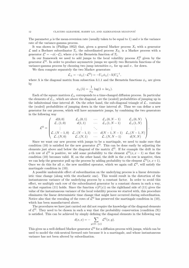
Each of the square matrices L± corresponds to a time-changed diffusion process. In particularthe elements of L+, which are above the diagonal, are the (scaled) probabilities of jumping up inthe infinitesimal time interval dt. On the other hand, the sub-diagonal triangle of L− containsthe (scaled) probabilities of jumping down in the time interval dt. Thus we can define a newgenerator for our process, which will have asymmetric jumps, by combining the two generatorsin the following way

LΩ =

d(0, 0) L+(0, 1) · · · L+(0, N − 1) L+(0, N)L−(1, 0) d(1, 1) · · · L+(1, N − 1) L+(1, N)

......

. . ....

...L−(N − 1, 0) L−(N − 1, 1) · · · d(N − 1, N − 1) L+(N − 1, N)L−(N, 0) L−(N, 1) · · · L−(N,N − 1) d(N,N)

.

Since we want our new process with jumps to be a martingale, we need to make sure thatcondition (10) is satisfied for the new generator LΩ. This can be done easily by adjusting theelements just above and below the diagonal of the matrix LΩ. If for example the drift in thex-th row of LΩ is positive, we add some probability to the element LΩ(x, x − 1) so that thecondition (10) becomes valid. If, on the other hand, the drift in the x-th row is negative, thenwe can help the generator pull up the process by adding probability to the element LΩ(x, x+1).Once we do this for all x, the new modified operator, which we again call LΩ, will satisfy themartingale condition in (10).

A possible undesirable effect of subordination on the underlying process is a linear determin-istic time change (along with the stochastic one). This would result in the distortion of theinstantaneous variance of the underlying process by a constant factor. In order to avoid thiseffect, we multiply each row of the subordinated generator by a constant chosen in such a way,so that equation (11) holds. Since the function v(F (x)) on the righthand side of (11) gives thevalue of the instantaneous variance of the local volatility process we started with, this procedureeliminates the linear deterministic time change that might have occurred during subordination.Notice also that the rescaling of the rows of LΩ has preserved the martingale condition in (10),which has been manufactured above.

The procedures we have just carried out did not require the knowledge of the diagonal elementsof LΩ. They need to be chosen in such a way that the probability conservation (condition (9))is satisfied. This can be achieved by simply defining the diagonal elements in the following way

d(x, x) = −∑

y∈Ω−x

LΩ(x, y).

This gives us a well-defined Markov generator LΩ for a diffusion process with jumps, which can beused to model the risk-neutral forward rate because it is a martingale, and whose instantaneousvariance has not been altered by subordination.


The construction we have just presented differs in two ways from the one in (Madan et al.1998). Firstly our time-changing approach is applicable to a general diffusion process which neednot be translation invariant17. Secondly we have the additional flexibility of specifying explicitlythe intensities of up-jumps and down-jumps separately.

3.3. Modelling the dynamics of stochastic volatility. In order to introduce the stochastic-ity of volatility into our modelling framework, we need to start with M ∈ N jump-diffusions ofsubsection 3.2 (all defined on the same domain Ω) which are given by Markov generators LΩ

α forα = 0, . . . ,M − 1. In this subsection we are going to define the dynamics of stochastic volatilitythat will give our model the ability to switch between the various jump-diffusion regimes. Aswill become clear, the stochasticity of volatility will be sensitive to the current level of the un-derlying, thus making it possible to relate the model to a particular view of the market. It is notuncommon among market participants to express market views (i.e. skew and smile behaviourof option prices) in terms of the future “levels” at which the underlying might be trading. Inour framework we can set these levels explicitly and are allowed to choose independently thecorresponding jump-diffusion, that can express the required view of the volatility surface. Theintroduction of stochastic volatility into the model will be in several stages. Let us start byspecifying the dynamics of stochastic volatility and then combining them with the underlyingjump-diffusion regimes to give a full specification of the model.

Let V be the set 0, . . . ,M − 1 of all possible volatility states. For each volatility state γ(in V ) we define a Markov generator GV

γ by specifying the matrix elements GVγ (α, β), for all

α, β ∈ V , so that the continuous-time diffusion given by GVγ mean-reverts to one of the volatility

states in V .We have defined M Markov generators GV

γ , each of them specifying its own dynamics ofthe stochastic volatility process. Our next task is to obtain a single global stochastic volatilityMarkov generator which will favour a certain regime γ conditional on the position of the forwardrate. This can be achieved by using a partition of unity which is described as follows. Choosea strictly increasing sequence Fγ of the forward rate levels so that, if the forward process isclose to the level Fγ , the market views of the smile and skew agree with the ones implied by theprocess LΩ

γ from subsection 3.2. The partition of unity is defined as a sequence of M functionsεγ : R → [0, 1] with the key property

m−1∑γ=0

εγ(F ) = 1, for all F ∈ R.

Given the sequence of levels Fγ , such functions can be defined explicitly, using a piecewise linearscheme, in the following way:

εγ(F ) :=

F−Fγ−1Fγ−Fγ−1

F ∈ [Fγ−1, Fγ ]Fγ+1−FFγ+1−Fγ

F ∈ [Fγ , Fγ+1]0 otherwise.

This definition has to be modified slightly for the boundary cases when γ equals 0 or (M − 1):

ε0(F ) :=

1 F ≤ F0F1−FF1−F0

F ∈ [F0, F1]0 F ≥ F1,

εm−1(F ) :=

0 F ≤ Fm−2

F−Fm−2Fm−1−Fm−2

F ∈ [Fm−2, Fm−1]1 F ≥ Fm−1.

We are now in a position to define our global Markov generator for the stochastic volatilityprocess, which has the capability of changing its properties when the forward rate undergoes a

17A key feature of Levy processes is that they are translation invariant. That is precisely the property of theBrownian motion with a drift required in the construction of the jump process in (Madan et al. 1998).


substantial move. The definition, using the partition of unity, goes as follows

LVx (α, β) :=

m−1∑γ=0

εγ(F (x))GVγ (α, β),

where α, β are elements in V and F (x) is the function on Ω describing the forward rate process.It follows from the defining property of partition of unity that the matrix LV

x is indeed a Markovgenerator for any element x of the underlying space Ω.

Just like with any stochastic volatility model, our aim is to define a Markov generator L whichwill specify the probabilities of going from any state (x, α) in Ω×V to any other state (y, β) (ofthe same set) in the infinitesimal time interval dt. The Markov generator L that specifies thedynamics of our model for the underlying forward rate is given by

L(x, α; y, β) := LΩα(x, y)δαβ + LV

x (α, β)δxy,(16)

where δ denotes the Kronecker delta function. Note that it follows trivially, from the propertiesof the Kronecker delta, that the matrix L is a genuine Markov generator (i.e. it has positiveentries off the diagonal and its rows sum to one). Another important feature is that the generatorL, by definition, does not allow for simultaneous jumps of the state and the volatility variables.This property ensures that our forward process FΩ

t , whose dynamics is specified by L, remainsa martingale:

E(x,α)t [dFΩ

t ] =∑

(y,β)∈Ω×V

(F (y)− F (x))(LΩ

α(x, y)δαβ + LVx (α, β)δxy

)=

∑y∈Ω

(F (y)− F (x))LΩα(x, y) + (F (x)− F (x))

∑β∈V

LVx (α, β) = 0.

3.4. Deterministic time-change. The model we have described so far is completely stationary.This amounts to the fact that the implied volatility surface is influenced purely by the modelparameters and has no explicit time dependence. By adjusting these parameters one can obtain ageneral shape of the market impled volatility surface and reprice correctly the out-of-the-moneyoptions.

In order to get a good match for the term structure of the at-the-money implied volatilitieswe have to introduce a minimal deterministic time-change, which only has a marginal effecton the out-of-the-money options. This adjustment can be specified by an increasing functionf : [0, T ] → [0,∞) which deterministically transforms calender time t to financial time f(t).Since our model can capture well the features of the underlying market before the deterministictime-change is introduced, the calender time t and the financial time f(t) will differ only slightlyfrom each other. We first find values of the function f for all market specified maturities bysatisfying the requirement that the at-the-money options are priced correctly. It will becomeclear in subsection 3.5 that a deterministic time-change plays a very isolated role in the pricingalgorithm. Therefore finding a correct value of f at the market specified maturities is not adifficult task. For all other times t we use a linear interpolation to arrive at the value f(t). Thegraph of the function f , used to calibrate the model to the market implied volatility surface forS&P 500, is given in figure 3.

3.5. Pricing and hedging of vanilla options and forward-starts. The pricing problem fora general European option expiring at time T reduces to the calculation of the transitional prob-ability density function p((x, α), t; (y, β), T ) for the underlying process FΩ

t , which was definedin subsection 3.3 via its Markov generator (16) (recall that (x, α), (y, β) are elements of Ω × Vwhile t is the current time). This is because our framework is defined in the risk-neutral measurewhich implies that the value of any security at time t equals the discounted expectation of thevalue of the same security at any time horizon T .

Since we would like to include the deterministic time-change of subsection 3.4 in the definitionof the density p((x, α), t; (y, β), T ), we must start by specifying the risk-neutral dynamics of the


underlying forward process in financial time. More precisely let

Us = (u((x, α), s; (y, β), S))(x,α),(y,β)∈Ω×V

be a stochastic matrix induced by the Markov generator L. In other words the coordinatefunctions u((x, α), s; (y, β), S) are the transition probabilities to go between the states (x, α) and(y, β) in the time interval [s, S]. The quantity s denotes the financial time and can therefore beexpressed as s = f(t), where f is the function from subsection 3.4 and t is the calendar time.Similarly S = f(T ) is the financial time horizon.

As was mentioned in subsection 3.1, the matrix Us satisfies the backward Kolmogorov18

equation (14) with the boundary condition US = I (I is the identity matrix on the vector spaceRk where k = m(N + 1)). The solution of the backward Kolmogorov equation can therefore beexpressed in terms of functional calculus as Us = exp((S − s)L) and can be calculated explicitlyusing the spectral decomposition of the operator L (which in this case is just k × k matrix) asgiven by (13). The first step is to calculate the eigenvalues λn of the Markov generator L andthe second is to find the eigenvectors un of L, put them into a transition matrix U , and findthe columns of the inverse U−1 which we will denote by vn. In section 4 we calibrate the modelusing a lattice with M(N + 1) = 5 · 76 = 380 points which implies that the generator L is asquare matrix of dimension 380× 380. For matrices of this size diagonalization routines such asdgeev in the numerical linear algebra library LAPACK are very efficient.

Once we have the spectral decomposition of L, we can calculate the probability kernelp((x, α), t; (y, β), T ), which depends on calender time, using functional calculus:

p((x, α), t; (y, β), T ) = e(f(T )−f(t))L((x, α), (y, β)) =M(N+1)∑

n=1

eλn(f(T )−f(t))un(x, α)vn(y, β).

Since we know that eigenvalues λn must have a negative real part, in the case of long-datedoptions only very few eigenvalues will play a role, because the exponential of a negative numberbecomes negligibly small very quickly. Another surprising and important fact which follows fromthe above representation of the probability kernel is that it depends in a very isolated way onthe (financial) time to maturity.

The current price Ct of a European derivative paying h(ST ) at the time horizon T , where St

is the underlying equity index, can be calculated in the following way

Ct(x, α) = e−(r(T )T−r(t)t)∑

(y,β)∈Ω×V

p((x, α), t; (y, β), T )h(e−(r(T )−d(T ))T F (y)).(17)

The point x from Ω is chosen in such a way so that the equation F (x) = e(r(t)−d(t))tSt holds,where St is the index level at the current time t, and α in V corresponds to the volatility regimewe are in at time t.

Our next task is to find the hedge-ratios for the derivative C0 within our model. It emergesthat this is a very simple matter which is not at all computationally demanding because all thehard numerical work has already been done by the pricing algorithm. The delta and the gammaof C0 are defined using symmetric differences in the following way

∆(x, α) :=C0(x + 1, α)− C0(x− 1, α)

F (x + 1)− F (x− 1)

Γ(x, α) := 4C0(x + 1, α) + C0(x− 1, α)− 2C0(x, α)

(F (x + 1)− F (x− 1))2,

where x is the lattice point in Ω that corresponds to the spot level of the index at time 0 (notethat at time 0 the spot is the same as the forward). Notice that calculating Ct(x + 1, α), or anyother value of the option Ct(y, α) with a starting point y different from x, requires no furtherdiagonalization because the pdf we need is given by a different row of the matrix Us, which has

18Notice that the Markov generator L in this equation acts on the coordinate functions of Us as a function ofthe variable (x, α).


already been calculated during the pricing of the original contract Ct(x, α). In fact if one requiresthe entire delta and gamma profiles of the derivative Ct (like the ones plotted in figures 4 and 5for call options struck at 100), the most efficient way of doing it is to use a general matrix-vectormultiplication routine gbmv from LAPACK and then piece together the corresponding Greeksusing the above formulae.

A similar procedure can be applied to obtain the vega of the contract Ct. Again we can defineit using a symmetric difference (in the stochastic volatility domain V ) with a formula

ν(x, α) :=C0(x, α + 1)− C0(x, α− 1)

σα+1 − σα−1,

that needs to be suitably amended in case we are in the volatility regime on the boundary ofthe domain V . The parameters σα, for α in the domain V , are the base volatilities in the CEVprocesses defined in subsection 3.1. Their values can be found in table 1. It is clear that thesame computational technique which yielded delta and gamma profiles can be used to find thevega profile of the derivative Ct (see figure 6 for the vega profile of call options with differentmaturities struck at 100).

Our final task is to find an algorithm for pricing forward starting options. Recall from sub-section 2.3 that the payoff of a forward-start is of the form (ST − aST ′)+, where T ′ < T area pair of maturities and a is the forward strike. Let us now assume that the current time is0 and let us reinterpret the formula (17), for t = T ′, as a forward price of the option contractwhich starts at the future time T ′ and expires at time T , conditional on the underlying equityindex being at the level ST ′ = e−(r(T ′)−d(T ′))T ′

F (x) and the whole system being in the volatilityregime α at time T ′. The payoff function in (17) is completely general and can therefore dependon the level of the underlying at T ′. In order to find the value of the forward-start at time T ′ wemust evaluate a portfolio of M(N +1) call options, one for each element (x, α) of the set Ω×V ,with the corresponding strikes ae−(r(T ′)−d(T ′))T ′

F (x) using formula (17). The most efficient wayof doing this is to collect all the call payoff functions into a matrix and apply a matrix-matrixmultiplication routine gemm (from LAPACK) on the forward probability kernel (between timesT ′ and T ) and the “payoff matrix” we have just created. Notice that both of these matrices aresquare and have dimension M(N + 1), which is hence also true of the product.

Let us now define the function h : Ω × V → R by requiring that h(x, α) equals the diagonalelement of the above product of matrices, which corresponds to the index (x, α). A moment’sreflection will show that the function h we have just defined equals the value of the forward-startat time T ′. In order to obtain the today’s value of the forward starting option, all we need todo is find the current value of the payoff h using expression (17).

We have therefore shown that pricing a forward-start in our framework amounts to one matrix-matrix multiplication and one matrix-vector multiplication. Similarly to the analysis of sensi-tivities that was carried out for European options earlier in this subsection, we could find delta,gamma, vega and other higher-order Greeks for the forward-starts. However we are not going topursue this any further; given the basic ideas we have already put forth, these algorithms wouldbe but trivial extensions.

4. Calibration to the vanilla surface

We are now going to calibrate the model for the underlying described in section 3 to theimplied volatility surface of the S&P 500 equity index for maturities between 3 months and 10years (see legend of figure 1 for all market defined maturities used in the calibration) and a broadrange of liquid strikes for each maturity. The market data consists of the implied Black-Scholesvolatilities for each strike and maturity19.

19Notice that we are using more strikes for longer maturities than for shorter maturities. This is not aninherent requirement but a consequence of the initial structure of the market data we used for calibration of themodel.


Our task is to find a set of values for the parameters of the model so that, if we repricethe above options and express their values in terms of the implied Black-Scholes volatilities,we reobtain the market quotes. The main calibration criterion is to minimize the explicit timedependence in order to preserve the correct (i.e. market implied) smile and skew through time.In other words the goal is to have the deterministic time-change function f from subsection 3.4 asclose to the identity transformation as possible. The stationarity requirement in the calibrationensures that the forward smile20 for any maturity still has the desired shape as can be observedin figures 7, 8, 9 and 10.

In order to calibrate our model we select an inhomogeneous grid with 71 = N + 1 pointswhich is used to span the possible values for the forward rate FΩ

t . We also choose M = 5 localvolatility regimes in order to capture the correct behaviour of the smile and skew of options onS&P 500.

It is well-known that in general the calibration problem is ill-posed and there is no guaranteethat there exists a unique solution. Our calibration strategy was based on an economic inter-pretation of the market data which gives a specific view of the smile behaviour in the future,conditional upon the underlying index trading inside (or breaking out of) certain “corridors”.Market makers often think in those terms when studying the possible scenarios and the effectthat they might have on their portfolio. Within our model these levels are set explicitly usingthe parameter Fα (see table 1). The desired market view (i.e. the shape of the smile conditionalon the underlying trading close to that level) can then be expressed by the appropriate choicefor the local volatility regime which is favoured by the stochastic vol process as described insubsection 3.3. The stochastic volatility process is given by the Markov generators GV

α whichare specified below. The short-dated end of the volatility surface (the so-called “gamma regime”of implied volatility) is, in case of the equity index, controlled by down-jump intensity ν−α .The long-dated part of the vol surface (i.e. the so-called “vega regime” of implied volatility) isregulated by the CEV parameters σα and βα as well as by the stochastic volatility generatorsGV

α .The set of parameters that was found to work best with the market data for the S&P 500

is reported in table 1. These parameters were discovered by following the guidelines above. Noattempts to automate these procedures have been made. It should be noted that, in case offinite-dimensional Markov generators it is easy to compute a clean gradient with respect to themodel parameters, which makes algorithms such as Levenberg-Marquardt square minimizingapproach easy to apply as long as one has a good starting point.

The S&P 500 index equaled 1195 at the time when the option data was recorded. Throughoutthe paper a relative value of the index, set at 100, is used for simplicity. The forward price levelsF (x), where x is an element of the underlying grid Ω, are also measured on the relative scale.Note also that our starting volatility regime is regime α = 2 and we therefore set F2 to be equalto 100. The values of the parameters βα are either negative or small and positive in order tokeep the skews of the corresponding local volatility regimes decreasing in strike. The choice ofthe parameters Fα (see table 1) implies that the smaller values of α correspond to the volatilityregimes which are more likely if the forward price is trading at a lower level. Therefore it isnatural to choose βα in such a way that it is an increasing function of α in order to account forthe recognized leverage effect which stipulates that the implied volatility levels are negativelycorrelated with the underlying.

5. Path-dependence and the lifting of a Markov generator

We have so far developed a model for the forward rate of the underlying index but have saidnothing about its realized variance. In the current section and the two that follow we are going

20There is a closed form solution for the value of a forward-start in the Black-Scholes model and the onlyunknown parameter in that formula is the forward volatility. It is therefore customary to define a forward smile

of any model as a function mapping the forward strike to the implied forward volatility which is obtained byinverting the Black-Sholes formula (see subsection 2.3 for the precise definition of a forward strike).


α σα βα σα ν−α ν+α Fα

0 27.0% -0.50 60% 0.50 0 50.001 15.5% -0.30 60% 0.40 0 90.002 12.5% -0.10 60% 0.35 0 100.003 15.5% 0.10 60% 0.25 0 110.004 27.0% 0.50 60% 0.04 0 150.00

Table 1. Parameters for the local volatility regimes and the jump intensities.

GV0 =

−4.75 4.75 0 0 03.25 −6.5 3.25 0 00 4.75 −8 3.25 00 0 4.75 −8 3.250 0 0 4.75 −4.75

, GV4 =

−4.75 4.75 0 0 03.25 −8 4.75 0 00 3.25 −8 4.75 00 0 3.25 −6.5 3.250 0 0 4.75 −4.75

Markov generators for stochastic volatility (α = 0, 4).

GVα =

−4.75 4.75 0 0 03.25 −8 4.75 0 00 3.25 −6.5 3.25 00 0 4.75 −8 3.250 0 0 4.75 −4.75

Markov generators for stochastic volatility (α = 1, 2, 3).

to build a mechanism that will make it possible to identify the random behaviour of the realizedvariance of the index. In order to do this we must return to the fundamental theory.

Let L be a generator for a continuous-time Markov chain Ft defined on a finite state spaceΩ. In other words the operator L is given by a square matrix (L(x, y))x,y∈Ω which satisfiesprobability conservation (9) and has non-negative elements off the diagonal. Each elementL(x, y) describes the first order change of the probability that the chain Ft (in this section wedrop the superscript Ω to simplify notation) jumps from level F (x) to the level F (y) in the timeinterval [t, t + dt], where the deterministic function F : Ω → (0,∞) is an injection which definesthe image of the process Ft.

Our aim in this section is to extend (i.e. lift) the generator L to the generator L, whichwill describe the dynamics of the lifting (Ft, It) of our original process Ft. The component It

will be a finite-state Markov chain, which we will describe shortly, that contains the relevantpath information, up to time t, of the underlying process Ft. The filtration associated with thelifting (Ft, It) will NOT contain any information that is not already available in the originalfiltration of the process Ft. In other words the extension (Ft, It) will be adapted to the filtrationgenerated by Ft. On the other hand the Markov generator of the lift (Ft, It) will give us theprobability kernel for the process It, which is what we are ultimately interested in as it containsthe probability distribution of the relevant path information.

We will start by describing a continuous process Σt which will contain the relevant path-information of the underlying Markov chain and then define a finite-state stochastic process It

that will be used to model Σt. The procedure we are about to describe works for a specific typeof path-dependence only. Assume that if at time t the underlying process Ft is at a state F (x)for some x ∈ Ω, then the change of the value Σt, in the infinitesimal time interval dt is of theform

dΣt = Q(x)dt,

where the function Q : Ω → R, defined in terms of the underlying stochastic process, has twokey properties:


• the mapping Q is independent of the path the underlying process follows on the interval[0, t) and

• the value Q(x) depends on the level x at time t and on the distribution of the underlyingprocess in the infinitesimal future time interval dt as given by the Markov generator L.

The first property states that the change in the path-information Σt, over a short time period[t, t + dt], does not depend on the path taken by the underlying process up to time t. Thesecond property tells us that the evolution of the path information over the interval [t, t + dt],conditional on the current level of the process Ft, is determined by the future distribution of Ft

over the infinitesimal time interval.It is clear that the realized variance of the process Ft up to time t, can be captured by a

random process Σt. Indeed, if we define the function Q in the following way

Q(x) :=∑y∈Ω

(F (y)− F (x)

F (x)

)2

L(x, y)(18)

it follows immediately that the above conditions are satisfied. This is because the realizedvariance of Ft is simply an integral over time of the instantaneous variance of Ft which is givenby (18).

The last observation is crucial for all that follows, because it implies that the process Σt isuniquely determined by its state-dependent instantaneous drift. In particular we see that theprocess Σt has no volatility and that it has continuous sample paths since it allows a represen-tation as an integral over time.

The fundamental consequence of these facts is the following: a finite-state Markov chain It canbe used as a model for the process Σt if and only if the instantaneous drift of the chain is equalto Q(x), whenever the underlying process Ft is in state F (x), and the instantaneous varianceof It is equal to zero up to first order. The first requirement clearly follows from the discussionabove. The second condition is there to reflect the fact that the process Σt is a continuous Itoprocess which has no volatility term. A non-constant random process on a lattice will alwayshave a non-zero instantaneous variance, but the second condition ensures that this instantaneousvariance goes to zero as quickly as the lattice spacing itself. In other words the Markov chainmodel It for Σt must exhibit neither diffusion nor jump behaviour.

5.1. Lifting of the generator for the underlying process. Recall that the Markov generatorL(x, y) for the underlying process in the forward measure, as described in section 3, is givenby (16). Here we have simplified the notation assuming that the variable x (resp. y) nowdenotes both the lattice value for the spot and the volatility level (the variable x (resp. y) runsover a set with M(N + 1) elements as defined in subsection 3.3).

Let It as above denote the Markov chain whose value approximates the realized variance Σt

of the forward price Ft from time 0 to time t. We shall express It as αmt where mt is a Poissonprocess (with non-constant intensity) starting at 0 and gradually jumping up along the gridgiven by 0, . . . , 2C, where C is an element in N. The constant α controls the spacing of thegrid for the realized variance It.

We are now going to specify precisely the dynamics of the process mt which is a fundamentalingredient of our model. As mentioned before, the process mt will behave as a Poisson pro-cess whose intensity is determined by the level of the underlying. In other words the Markovgenerator, conditional on the underlying process being at the level F (x), is of the form

Lm(x : c, d) :=

1αQ(x) if d = (c + 1) mod (2C + 1);

− 1αQ(x) if d = c.

(19)

The variables c and d are elements of the discrete set 0, . . . , 2C and the function Q is theinstantaneous variance of the underlying process as defined in (18). This family of generators


specifies the dynamics of the process It with the following instantaneous drift

lim∆t→0

E[It+∆t − It

∆t

∣∣∣Ft = F (x), It = I(c)]

=2C∑d=0

(I(d)− I(c))Lm(x : c, d)

= α(c + 1− c)1α

Q(x) = Q(x),(20)

for all values F (x) of the underlying process Ft and all integers c which are strictly smallerthan 2C. This implies that the Markov chain It has the same instantaneous drift as the actualrealized variance. A similar calculation tells us that the instantaneous variance of It equalsαQ(x). Since α is the spacing of the lattice for the chain It, we have just shown that the firsttwo instantaneous moments of It match the first two moments of the realized variance Σt for allpoints on the lattice 0, . . . , 2C except the last one.

Notice however that the equality (20) breaks down if c equals 2C, because we have imposedperiodic boundary condition for the process It. Put differently this means that It is in fact aprocess on a circle rather than on an interval. The latter would be achieved if we had imposedabsorbing boundary conditions at 2C. That would perhaps be a more natural thing to do sincethe process Σt is certainly not periodic. But an absorbing boundary condition would destroy thedelicate structure of the spectrum of the lifted generator L which is preserved by the periodicboundary condition. It is precisely this structure that makes the periodic nature of It a keyingredient of our model, because it allows us to linearize the complexity of the pricing algorithm,as we shall see in section 6. It should be noted that the general philosophy behind either choiceof the boundary condition would be the same: the lattice in the calibrated model should be setup in such a way that the process never reaches the boundary value 2C, because if it does aninevitable loss of information will ensue regardless of the boundary conditions we choose.

We are now finally in a position to define the lifted Markov generator of the process (Ft, It)as

L(x, c; y, d) := L(x, y)δc,d + Lm(x : c, d)δx,y.(21)

The structure of the spectrum of the operator L will be exploited in section 7 to obtain apricing algorithm for payoffs which are general functions of the realized variance. The reason forspecifying the generator Lm(x : c, d) by (19) (i.e. insisting on the periodic boundary conditionfor the process It) will become clear in section 6 when we explore the spectral properties of thelifted generator L.

6. Diagonalization algorithm for partial-circulant matrices

In this section our aim is to generalize a known diagonalization method from linear algebrawhich will yield a numerically efficient algorithm for obtaining the joint probability distributionof the spot and realized variance at any maturity. Let us start with some well-known concepts.

A matrix C ∈ Rn×n is circulant if it is of the form

C =

c0 c1 c2 · · · cn−1

cn−1 c0 c1 · · · cn−2

cn−2 cn−1 c0. . .

......

.... . . . . . c1

c1 c2 · · · cn−1 c0

,

where each row is a cyclic permutation of the row above. The structure of matrix C can also beexpressed as

Cij = c(i−j) mod n,


where Cij is the entry in the i-th row and j-th column of matrix C. It is clear that any circulantmatrix is a Toeplitz21 operator and in fact circulant matrices are used to approximate generalToeplitz matrices and explain the asymptotic behaviour of their spectra. We will not investigatethis idea any further (for more information on the topic see (Bottcher & Silbermann 2006)) sinceour main interest lies in a different generalization of circulant matrices, namely that of partial-circulant matrices, which will be defined in subsection 6.2. Before doing that we are going torecall some of the known properties of circulant matrices.

6.1. Eigenvalues and eigenvectors of circulant matrices. Let C denote a circulant matrixof dimension n as defined above. The eigenvalue λ and the eigenvector y ∈ Rn are the solutionsof the equation Cy = λy, which is equivalent to the system of n linear difference equations withconstant coefficients:

n−1∑k=o

ckyk = λy0 and

j−1∑k=0

cn−j+kyk +n−1∑k=j

ck−jyk = λyj , for j ∈ 1, . . . , n− 1.

The variables yk, for k ∈ 0, . . . , n − 1, in these equations are simply the coordinates of theeigenvector y. Such systems are routinely solved by guessing the solution and proving that itis correct (see appendix 1 in (Grimmett & Stirzaker 2001)). The solution in this case is of theform

λ =n−1∑k=0

ckzk and yj =zj

√n

for j ∈ 0, . . . , n− 1,

where z is a complex number which satisfies zn = 1. This implies that the eigenvalue-eigenvectorpairs of matrix C are parameterized by the n-th roots of unity which are of the form zr =exp(−2πir/n), where the index r lies in 0, . . . , n − 1 and i is the imaginary unit. Thereforethe j-th coordinate of the r-th eigenvector, together with the corresponding eigenvalue, can beexpressed as

y(r)j =

1√n

e−i 2πn rj and(22)

λr =n−1∑k=0

cke−i 2πn rk for r, j ∈ 0, . . . , n− 1.(23)

This representation is extremely useful because it allows us to deduce a number of fundamentalfacts about circulant matrices. Let us start with the eigenvectors. It is obvious that if we put alln vectors y(r) side by side into a matrix, the determinant of the linear operator obtained is theVandermonde determinant, which is non-zero since its parameters are the n distinct solutions ofthe equation zn = 1. This implies that matrix C can be diagonalized and that all its eigenvectorsare of the form (22).

Another key property of circulant matrices is that they can all be diagonalized using the sameset of eigenvectors. This follows directly from (22) since the expression for the vectors y(r) areclearly independent of matrix C.

Expression (23) tells us that the r-th eigenvalue of C equals the value (at the point r) of thediscrete Fourier transform (DFT) of the sequence (cj)j=0,...,n−1. We can therefore recover thesequence (cj) from the spectrum (λr)r=0,...,n−1 of C using the inverse discrete Fourier transform.Even though this is a very well-known and celebrated fact, we will now present a short proof forit, because the argument itself sheds light on the behaviour of circulant matrices.

21For definition see for example (Bottcher & Silbermann 2006). Toeplitz operators arise in many contextsin theory and practice and therefore constitute one of the most important classes of non-self-adjoint operators.They provide a setting for a fruitful interplay between operator theory, complex analysis and Banach algebras.


Note that for any index k ∈ Z, such that (k mod n) is different from zero, we obtainn−1∑r=0

ei 2πn rk =

1− ei 2πn kn

1− ei 2πn k

= 0,(24)

by summing a finite geometric series. In particular this implies that the above sum for anyk ∈ Z equals nδ1,k mod n, where δ is the Kronecker delta which takes value 1 at zero and value0 everywhere else. The inversion formula for the DFT is now an easy consequence

1n

n−1∑r=0

λrei 2π

n rl =1n

n−1∑r=0

n−1∑k=0

(cke−i 2π

n rk)

ei 2πn rl

=n−1∑k=0

ck1n

n−1∑r=0

ei 2πn r(l−k) = cl,

for any l in 0, . . . , n − 1. Before proceeding we should note that the argument we have justoutlined implies that a circulant matrix is uniquely22 determined by its spectrum.

Another consequence of the extraordinary identity (24) is that for any pair of distinct indicesk and r in 0, . . . , n− 1, the corresponding eigenvectors y(k) and y(r) are perpendicular to eachother. Since we have chosen the vectors y(r) in (22) so that their norm is one, the set of alleigenvectors of a circulant matrix is an orthonormal basis of the vector space Cn.

Let A be another circulant matrix given by the sequence (ak)k=0,...,n−1 with the spectrum(αr)r=0,...,n−1. Since A and C can be diagonalized simultaneously using the basis y(r); r =0, . . . , n−1, it follows that the product AC is also diagonal in this basis and that its eigenvaluesare of the form αrλr. Therefore AC is a circulant matrix whose first row equals the convolution23

of the sequences (ak) and (ck). The diagonal representation also implies that the matrices Aand C commute. Finally note that the sum A + C is also a circulant matrix.

6.2. Partial-circulant matrices. We are now going to define a class of matrices, that willinclude the Markov generator given by (21), which can be diagonalized by the semi-analyticalgorithm from subsection 6.4.

Let A be a linear operator represented by a matrix in Rm×m and let B(k), for k = 0, . . . ,m−1,be a family of n-dimensional matrices with the following property: there exists an invertiblematrix U ∈ Cn×n such that

U−1B(k)U = Λ(k), for all k ∈ 0, . . . ,m− 1,where Λ(k) is a diagonal matrix in Cn×n. In other words this condition stipulates that thefamily of matrices B(k) can be simultaneously diagonalized by the transformation U . Thereforethe columns of matrix U are eigenvectors of B(k) for all k between 0 and m− 1.

Let us now define a large linear operator A, acting on a vector space of dimension mn, in thefollowing way. Clearly matrix A can be decomposed naturally into m2 blocks of size n× n. LetAi,j denote an n× n matrix which represents the block in the i-th row and j-th column of thisdecomposition. We now define the operator A as

Aii := B(i) + AiiIRn and(25)

Aij := AijIRn , for all i, j ∈ 1, . . . ,m such that i 6= j.(26)

The real numbers Aij are the entries of matrix A and IRn is the identity operator on Rn. Wemay now state our main definition.Definition. A matrix is termed partial-circulant if it admits a structural decomposition asin (25) and (26) for any matrix A ∈ Rm×m and a family of n-dimensional circulant matricesB(k), for k = 0, . . . ,m− 1.

22Such a statement is untrue even for self-adjoint and unitary operators.23Recall that the DFT of the convolution of two sequences equals the product of the DFTs of each of the

sequences.


The concept of a partial-circulant matrix is well-defined because, as we have seen in subsec-tion 6.1, any family of circulant matrices can be diagonalized by a unitary transformation whosecolumns consist of vectors y(r), for r between 0 and n− 1 (see equation (22)).

The operator A is very big indeed. The typical values that are of interest to us for thedimensions m and n are 70 and 600 respectively. This implies that matrix A contains (70 ·600)2,i.e. more than one billion, entries. This means that even storing A on a computer requires about10 Gb of memory.

Our task is to find the spectrum of the operator A. Given its size and the fact that it isnot a sparse matrix, this problem at first sight appears not to be tractable. But the structureof matrix A, combined with the ubiquitous idea of invariant subspaces of linear operators, willyield the solution. We will describe the diagonalization algorithm for partial-circulant matricesin subsection 6.4. Before we do this we need to recall the basic properties of invariant subspaces.

6.3. Invariant subspaces of linear operators. Let A : V → V be a linear operator on afinite-dimensional vector space V . By definition a subspace X of V is an invariant subspace ofthe operator A if and only if AX ⊆ X. Note that the set AX is a subspace of V . It is clearfrom the definition that vector spaces 0, V , AV and ker(A) are all invariant subspaces of theoperator A. Another trivial example is the space of all eigenvectors of A that belong to aneigenvalue λ.

It is the non-trivial examples however that make this concept so powerful. If we can findtwo invariant subspaces X1 and X2 of V for the operator A, such that X1 ∩ X2 = 0 anddim X1 + dim X2 = dim V (i.e. V = X1 ⊕ X2), then in the appropriate basis the matrixrepresenting the operator A takes the form

D =(

A1 00 A2

),

where A1 (resp. A2) is the matrix acting on the subspace X1 (resp. X2). The zeros in theabove expression represent trivial linear operators that map the subspace X1 into the origin ofthe subspace X2 and vice versa.

The advantage of this structural decomposition of the original operator A is clear becauseit reduces the dimensionality of the problem. The spectral decomposition (i.e. the eigenvaluesand eigenvectors) of A can now be obtained from the spectral decomposition of two smalleroperators A1 and A2. Block-diagonalization consists of finding the transition matrix F (i.e. theappropriate coordinate change) that will transform the original matrix A into block-diagonalform given by matrix D above:

F−1AF = D.

6.4. Algorithm for block-diagonalization. Let A be the linear operator defined in (25)and (26) which acts on the vector space Cmn. We are now going to describe the block-diagonalization algorithm for A. In other words we are going to find invariant subspaces Vj

of the operator A (where j ranges between 1 and n), such that Cmn = V1 ⊕ · · · ⊕ Vn, and atransition matrix F ∈ Cmn×mn, such that the only non-zero n× n blocks of matrix F−1AF arethe diagonal ones.

Recall that, by definition of A, there exists a matrix U ∈ Cn×n consisting of eigenvectors forthe matrices B(k). Put differently the columns uj ∈ Cn, for j = 1, . . . , n, of U satisfy the identity

B(k)uj = λ(k)j uj for k ∈ 0, . . . ,m− 1.

Now fix any index j between 1 and n and define vectors v(j)i ∈ Cmn, where i = 1, . . . ,m, as

follows:

v(j)i := (0, . . . , 0︸︷︷︸

(i−1)n

, u′j , 0, . . . , 0︸︷︷︸(m−i)n

)′,(27)


where u′j is a row of n complex numbers obtained by transposing and conjugating the vector uj .

We can now define the subspace Vj of Cmn as the linear span of vectors v(j)i . It is clear that the

intersection of subspaces Vj and Vk is trivial for any two distinct indices j, k ∈ 1, . . . , n. This isbecause the eigenvectors uj and uk are linearly independent in Cn since, by assumption, matrixU is invertible. It follows directly from the definition that the dimension of Vj is m. Since thereare exactly n subspaces Vj , we obtain the decomposition Cmn = V1 ⊕ · · · ⊕ Vn.

If we manage to show that each space Vj is an invariant subspace for the operator A, wewill be able to conclude that A can be expressed in the block-diagonal form as described insubsection 6.3. Since the subspace Vj is defined as a linear span of a set of vectors v(j)

i ; i =1, . . . ,m, the invariance property AVj ⊆ Vj will follow if we demonstrate that the vector Av

(j)i

is in Vj for all i = 1, . . . ,m. By definition of A ((25) and (26)) it immediately follows that

Av(j)i =

m∑k=1

Aikv(j)k + λ

(i−1)j v

(j)i for i ∈ 1, . . . ,m,(28)

where λ(i−1)j is the eigenvalue of matrix B(i−1) that corresponds to the eigenvector uj and the

real numbers Aki are the entries of matrix A ∈ Rm×m. Identity (28) implies that each subspaceVj is an invariant subspace for A. Furthermore, if we define a matrix F ∈ Cmn×mn in thefollowing way

F :=(v(1)1 , . . . , v(1)

m , v(2)1 , . . . , v(2)

m , . . . , v(n)1 , . . . , v(n)

m

),(29)

then matrix D = F−1AF is block-diagonal. In other words if we decompose D into n2 matricesDij of size m×m, then the following formula holds

Dij = δij(A + Θ(j)) for i, j ∈ 1, . . . , n,(30)

where Θ(j) is a diagonal matrix in Cm×m with its i-th diagonal element equal to λ(i−1)j . As

usual the symbol δij denotes the Kronecker delta function.Expression (30) gives us the block-diagonal representation of the operator A. Notice that

the diagonal elements of matrix Θ(j) are precisely the eigenvalues of matrices B(i), for i =0, . . . ,m− 1, that correspond to the eigenvector uj .

The algorithm to block-diagonalize the operator A, defined by matrices A ∈ Rm×m andB(k) ∈ Rn×n (see (25) and (26)), can now be described as follows:

(I) Find matrix U ∈ Cn×n whose columns are the common eigenvectors uj , for j ∈ 1, . . . , n,of the family B(k).

(II) Construct the transition matrix F using the columns of matrix U as described in (27)and (29).

(III) Find the eigenvalues λ(k)j which satisfy B(k)uj = λ

(k)j uj for k ∈ 0, . . . ,m − 1 and

j ∈ 1, . . . , n.(IV) Construct diagonal matrices Θ(j) ∈ Cm×m, for all j ∈ 1, . . . , n, given by Θ(j)

ik =δikλ

(i−1)j , where the indices i, k run over the set 1, . . . ,m.

(V) Construct the block-diagonal representative D for the operator A as described in (30).

Our main task is to find the spectrum of matrix A. Notice that, since the spectrum of A isa union of the spectra of A + Θ(j), this algorithm has reduced the problem of diagonalizing annm × nm matrix to finding the spectra of n matrices of size m × m. The algorithm providesa key step for our pricing method because it enables us to model the behaviour of the realizedvariance by increasing the numerical complexity only linearly .

We should also note that in the case of the lifted Markov generator L in (21), matrix A isthe generator L of the underlying process while the family B(k) consists of circulant matrices.


In other words the operator L is given by a partial-circulant matrix. It therefore follows fromthe discussion in subsection 6.1 that the columns of the corresponding transition matrix F arepairwise orthogonal and that the entries of matrix LF are the values of a partial24 discreteFourier transform of the rows of L. This simple observation will be useful when calculating theprobability kernel of the lifted generator in the next section.

7. Pricing of derivatives on realized variance

Let ΣT be the realized variance over the time interval [0, T ], expressed in annual terms, asdefined in (1). In this section we are going to find pricing formulae, analogous to those given insubsection 3.5, for general payoffs that depend on the annualized realized variance ΣT .

Our first task is to find the probability kernel of the lifted process (Ft, It) which was defined insection 5. Recall that the Markov chain It = αmt, which is used to model the realized variance,is specified in terms of a translation invariant process mt, whose domain is Ψ = 0, . . . , 2C,and some positive constant α which determines the lattice spacing for the domain of It. Thevalue C ∈ N specifies the size of the lattice for the realized variance and has to be large enoughso that the process It, starting from zero, does not transverse the entire lattice. This is a veryimportant technical requirement as it ensures that there is no probability leakage in the model(which is theoretically possible since we are using periodic boundary conditions for the processIt). The dynamics of the chain mt are given by the Markov generator in (19).

Recall also that the process It records the total realized variance up to time t, which impliesthat the annualized realized variance ΣT that interests us, will be described by 1

T IT where thetime horizon T is expressed in years. The key ingredient in the calculation of the probabilitydistribution function of the process (Ft, It) is the block-diagonalization algorithm from subsec-tion 6.4. We are now going to apply it to the generator (21) in order to find the joint pdf of thelifted process.

7.1. Probability kernel of the lift (Ft, It). We saw at the end of section 6 that the generatorL(x, β, c; y, γ, d) of the process (Ft, It), given by (21), is a square partial-circulant matrix actingon a vector space of dimension M(N + 1)(2C + 1). The coordinates (x, β, c), (y, γ, d) of thematrix L (i.e. the lattice points of the process) lie in the set Ω × V × Ψ, where Ω is the gridfor the underlying forward rate and the set V contains all volatility regimes of the model (seesection 3 for a precise definition). Notice that the circulant matrices Lm from (19), used in thedefinition of L, are very simple because the only non-zero elements are on the diagonal, justabove the diagonal and the element in the bottom left corner of the matrix. In other words ifwe interpret the matrix Lm, associated with the lattice point (x, β), in terms of the definition ofa circulant matrix given at the beginning of section 6, we see that

c1 = −c0 =Q(x, β)

α,

where the function Q(x, β) is the instantaneous variance as defined by (18) and the constant αis the lattice spacing of the domain of It. All other elements cj are equal to zero.

It is therefore clear that, using the expression (23) for the eigenvalues of circulant matrices,equation (30) can be reinterpreted as

Lk(x, β; y, γ) := L(x, β; y, γ) + δ(x,β),(y,γ)

(e−ipk − 1

) Q(x, β)α

,

where Lk is the k-th block in the block-diagonal decomposition of L and the value of pk is givenby the expression

pk :=2π

2C + 1k.(31)

24Since each row of matrix L is naturally described by two variables, namely the value of the underlying andthe value of the realized variance, partial DFT is by definition a DFT acting on the second variable.


The index k in these expressions runs from 0 to 2C. Notice that the matrices Lk differ from theMarkov generator L only along the diagonal. We are now in a position to state the key theoremthat will allow us to find the probability kernel of the lifted process.

Theorem 7.1. Let L be the Markov generator of the stochastic process (Ft, It) as described insection 5 and let φ : C → C be a holomorphic function. Then the following equality holds

φ(L)(x, β, c; y, γ, d) =1

2C + 1

2C∑k=0

e−ipk(c−d)φ(Lk)(x, β; y, γ),

where Lk is the operator defined above, pk is given by (31) and (x, β, c), (y, γ, d) are elements ofΩ× V ×Ψ.

Before embarking on the proof of this theorem we may summarize as follows: if a linearoperator A can be block-diagonalized by a discrete Fourier transform (cf. last paragraph ofsubsection 6.4), then so can any operator φ(A) where φ is a holomorphic function defined onthe entire complex plane. Note that the assumptions on function φ and the linear operator L intheorem 7.1 are too stringent and in fact the theorem holds in much greater generality. For ourpurposes however the setting described in the theorem is sufficient as it applies directly to themodel. We will therefore only give a proof of the restricted case stated above.Proof. Let us start by recalling that any holomorphic function defined on C has a Taylor expan-sion around zero that converges everywhere. We can therefore define φ(A), via expression (13),for any linear operator A on a finite-dimensional vector space. It also follows from the fact thatφ has a Taylor expansion that any invariant subspace (see subsection 6.3 for definition) of A isalso an invariant subspace of φ(A). In particular if A has a block-diagonal decomposition in thesense of subsection 6.4, then the matrix φ(A) also has one. Moreover if B is a block in A thenφ(B) must be a block in φ(A).

We know that the Markov generator L can be expressed as L = FDF−1, where D is ablock-diagonal matrix of the form

D =

L0 0 · · · 00 L1 · · · 0...

.... . .

...0 0 · · · L2C

,

and the transition matrix F is given by (29). We have just seen that φ(D) must therefore alsobe in block-diagonal form:

φ(D) =

φ(L0) 0 · · · 0

0 φ(L1) · · · 0...

.... . .

...0 0 · · · φ(L2C)

.

It is clear from definition (13) and the power series expansion of φ that φ(L) = Fφ(D)F−1.Since matrix F is defined using the eigenvectors of circulant matrices, it follows immediately thatthe inverse F−1 can be obtained by transposing F and conjugating each of its elements. Note thatthe dimension of our circulant matrices is 2C + 1 and express φ(L)(x, β, c; y, γ, d) = 〈u, φ(D)v〉as a real inner product of two vectors u and φ(D)v, where u equals the (x, β, c)-row of the matrixF and v is the (y, γ, d)-column of F−1 (i.e. the conjugated (y, γ, d)-row of F ).

It follows from the definition of F and the above expression for φ(D) that the non-zerocoordinates of the vector u are of the form

1√2C + 1

e−ipkc


for all k ∈ Ψ and that the corresponding coordinates of φ(D)v are

1√2C + 1

eipkdφ(Lk)(x, β; y, γ).

The equality in the theorem now follows directly from the expressions for the coordinates of thevectors u and φ(D)v and the definition of the real inner product. This concludes the proof ofthe theorem. 2

We can now find the full probability kernel of the process (Ft, It) by applying theorem 7.1and then using the same procedure as in subsection 3.5. More explicitly, for any pair of calendartimes t and T , such that t < T , we have

p((x, β, c), t; (y, γ, d), T ) = e(f(T )−f(t))L(x, β, c; y, γ, d)

=1

2C + 1

2C∑k=0

e−ipk(c−d)e(f(T )−f(t))Lk(x, β; y, γ)

=1

2C + 1

2C∑k=0

M(N+1)∑n=1

eλkn(f(T )−f(t))e−ipk(c−d)uk

n(x, β)vkn(y, γ),(32)

where λkn are the eigenvalues and uk

n are the eigenvectors of Lk. As usual we denote by vkn the

columns of the matrix U−1k , where Uk consists of all the eigenvectors of Lk. Function f in the

above formula is the deterministic time-change for the underlying model which was introducedin subsection 3.4.

Formula (32) is our key result because it allows us to price any derivative which dependsjointly on the realized variance of the underlying index and the index itself at any time horizonT . In subsection 7.2 we find explicit formulae for the values of such derivatives using the jointprobability distribution function (32).

Figures 13, 14, 15, 16, 17 and 18 contain the graphs of joint distribution functions of thespot level and the annualized realized variance for maturities between 6 months and 5 years.The marginal distributions of the annualized realized variance, obtained from the above jointdistributions by integration in the dimension of the spot value of the index, are shown in figure 11.

The parameters in the model that influence the dynamics of the realized variance It are thenumber of lattice points C and the lattice spacing α. Table 2 contains their values for differentmaturities. It should be noted that the numerical complexity of the algorithm used to obtain

6m 1y 2y 3y 4y 5yC 80 80 100 90 100 110α 0.0002 0.0004 0.0009 0.0017 0.0021 0.025

Table 2. Parameters specifying the geometry of the lattice for the realizedvariance process It.

the pdf of the joint process (Ft, It) grows linearly with C. As mentioned earlier, it is crucialthat the value of C be chosen large enough with respect to the spacing α so that the processcannot get to the other side of the lattice with positive probability. Having arrived at the pdfin (32), our next task is to find the value of any derivative whose payoff depends on the realizedvariance.

7.2. Pricing derivatives on the realized variance. Let us assume that we are given a generalpayoff h(ΣT−t) that depends on the annualized realized variance ΣT−t between the current timet and some future expiry date T . The current price of a derivative with this payoff within ourmodel can be computed directly using the joint probability distribution function (32) in the


following way

Ct(x, β) = e−(r(T )T−r(t)t)∑d∈Ψ

∑(y,γ)∈Ω×V

p((x, β, 0), t; (y, γ, d), T )

h

(αd

T − t

).

The sum in the brackets is the marginal distribution of the process It at time T − t. Noticethat the realized variance process must always start from 0 at the inception of the contract. Thefactor 1

T−t normalizes the value of IT−t so that it is expressed in annual terms. As before, theconstant α is the lattice spacing for the realized variance.

The point x from Ω is chosen in such a way that the equation F (x) = e(r(t)−d(t))tSt holds,where St is the index level at the current time t, and β in V corresponds to the volatility regimeat time t.

Notice that because in the valuation formula above there is no restriction on the payofffunction h, the contract Ct can be anything from a variance swaption to a volatility swap (orswaption) and can be priced almost instantaneously using the calibrated model.

8. Some numerical results

Let us now use the calibrated model together with the pricing and hedging algorithms de-scribed in subsection 3.5 and sections 6 and 7 to perform some numerical experiments andconsistency checks for vanilla options, forward-starts and variance swaps.

8.1. Profiles of the Greeks. In order to test the pricing methodology of the model for theunderlying forward rate we pick a strip of call options with the same notional but with varyingmaturities, all struck at the current spot level. Since the entire framework for the underlyingis expressed in relative terms with respect to the current value of the index, the strike used forthis strip of options is 100.

Because we are interested in the behaviour of our pricing algorithm in changing marketconditions, we are going to study the properties of the first-order sensitivities to the marketparameters of our options with respect to all possible spot levels. In other words we are goingto calculate delta, gamma and vega, using the definitions given in subsection 3.5, as functionsof the current spot level.

This task does not pose any additional numerical difficulties because all it requires is theknowledge of the probability distribution functions of the underlying at the relevant maturitiesconditional upon the starting level, which can be any of the points in the grid. But if we havealready priced a single option, then these pdfs are available to us without any further numericalefforts. This is because, when pricing an option, the algorithm described in subsection 3.5calculates the entire probability kernel for each starting point in the grid, even though theoption pricing formula only requires one row of the final result. In this situation we requireall the rows of the probability kernel so as to obtain the prices of our option, conditional upondifferent spot levels, by applying the matrix of the kernel to the vector whose coordinates arevalues of the payoff calculated at all lattice points. As defined in subsection 3.5, the Greeks arelinear combinations of the coordinates of the final result of the calculation.

Figure 4 contains the delta profile of the call options for different maturities. Figures 5 and 6give the gamma and the vega profiles of the call options in the strip. As expected, an owner ofa vanilla option is both long gamma and long vega. The shapes of the graphs in figures 5 and 6also confirm that, according to our model, the at-the-money options have the largest possiblevega and gamma for any given maturity. A cursory inspection of the scales of gamma and vegafor options with the same notional indicates that in our model some calender spreads25 can besimultaneously long vega and short gamma or vice versa.

25A calendar spread is a structure defined by going long one call option and going short another call optionof the same strike but different maturity.


8.2. Forward smile. In subsection 2.3 we defined the concept of forward volatility using theBlack-Scholes formula for the forward starting options. One of the parameters in this formulais a forward strike. Any model for the underlying process defines a functional relationshipbetween forward strikes and implied forward volatilities using the Black-Scholes pricing formulafor forward-starts, in much the same way as it defines the implied volatility as a function ofstrike. This functional relationship is know as the forward smile.

The reason why the forward smile is so important lies in the fact that it determines theconditional behaviour of the process. It is well-known that knowing all the vanilla prices (i.e. theentire implied volatility surface) is not enough to price path-dependent exotic options. In termsof stochastic processes this statement can be expressed by saying that knowing the probabilitydistributions of the underlying for all maturities does not determine the process uniquely, noteven up to sets of probability zero. The forward smile contains the information about the two-dimensional distributions of the underlying process. In other words one can have two differentmodels that are perfectly calibrated to the implied volatility surface but which assign completelydifferent values to the forward starting options.

Market participants can express their views on the two-dimensional distributions of the un-derlying process by setting the prices of the forward starting options accordingly. It is thereforeof utmost importance for any model used for pricing path-dependent derivatives to have theimplied forward smiles close to the ones implied by the market. Unfortunately we did not havethe market implied forward volatilities that were prevailing at the time when the S&P 500 vanillaoptions data was recorded. Figures 7, 8, 9 and 10 contain the forward smiles implied by ourmodel for maturities between 3 months and 2 years. Since we have no market data to com-pare them with, we can only say that the qualitative nature of the implied forward smiles isas expected in the following sense: for a fixed time T ′ the forward smiles are flattening withincreasing T (for definition of times T ′ and T see subsection 2.3) and for a fixed difference T −T ′

the shapes of the forward smiles look similar when compared across maturities T ′. It should benoted that the latter point exemplifies the stationary nature of the underlying model and showsthat we did not have to use extreme values of the model parameters to calibrate it to the entireimplied volatility surface, because the two-dimensional distributions of the underlying processhave some of the necessary features which are expected by the market participants.

We should also note that a statistical comparison of the forward volatility smiles implied bythe model and by the market can be carried out easily because, as was mentioned at the endof subsection 3.5, pricing a forward starting option consists of two consecutive linear algebraoperations which require little computing time.

8.3. Probability distribution for the implied volatility index. One of our goals in thispaper has been to describe the random evolution of VIX through time. In figure 20 we plot theprobability distribution functions of the volatility index, as defined at the end of subsection 2.3.It is clear from these graphs that the future behaviour of the portfolio of options defining VIX ismodel-dependent. It is not hard to see that the peaks of the distributions in figure 20 are closeto the values of the model parameter σα (see section 4 for definition) which is used to definedifferent local volatility regimes. This can be explained by recalling that the stochasticity ofvolatility in our model does not (on average) influence the behaviour of the underlying processin time horizons as short as one month. Therefore the process is very likely to stay within thesame local volatility regime for a month after it hits any of the maturities in figure 20. Thisclaim is substantiated by the graphs in figure 21 which exhibit much more regular behaviour(i.e. there are no local maxima) if we monitor the same portfolio as the one in the definition ofthe volatility index but over a longer time period.

Since we can calculate explicitly distributions of VIX for any maturity (like those in figure 20),pricing a European option on the VIX in our framework amounts to summing the values of thepayoff against the pdf in the same way as was done for European payoffs on the underlying indexin (17) of subsection 3.5.


8.4. Distribution of the realized variance. Most of the modelling exercise presented sofar has been directed towards finding the probability distribution function for the annualizedrealized variance of the underlying process. Figure 11 contains the pdfs for the realized variancefor maturities between 6 months and 5 years as implied by the model that was calibrated to themarket data for the S&P 500. The corresponding term structure of the fair values of varianceswaps for these maturities is given in figure 19. This term structure is obtained by calculating theexpectation (in the risk-neutral measure) of the probability distribution functions of figure 11.

Figure 19 also contains the current value of the logarithmic payoff, as given by (5), for theabove maturities. In (Demeterfi et al. 1999b) the performance of the log payoff as a hedgeinstrument for the variance swap is studied in the presence of a single down-jump throughoutthe life of the contract. In equation 42 the authors show that, in this case, the log payoff is worthmore than the variance swap. Note that the values of the log payoff in figure 19 dominate thevalues of the variance swaps, as given by our model. This agrees with (Demeterfi et al. 1999b)because our underlying model is among other things an infinite activity jump process with zerointensity for up-jumps. Note also that the effect of jumps forces the price difference between thevariance swap and the log payoff to grow with time. This may appear counterintuitive at firstbecause, in the context of the implied volatility smile, one is accustomed to jump effects fadingaway with time. In this case however the realized variance is cumulative and, with respect toa 5 year variance swap, jumps that occur in 3 years time are equally important to jumps thathappen in a week’s time. This accounts for the divergent behaviour in figure 19.

As was mentioned in the introduction, the class of HJM-like models for volatility derivatives(see for example (Buehler 2006)) require an entire term structure of variance swaps (like theone in figure 19) to be calibrated. Our approach on the other hand implies one from the vanillaoptions data (and of course some modelling hypothesis). Note also that joint pdfs for the realizedvariance and the underlying index are given in figures 13, 14, 15, 16, 17 and 18.

8.5. The log contract and variance swaps in a market without jumps. It is well-knownthat in a market where the underlying follows a continuous stochastic process the fair value of avariance swap is equal to the value of the replicating European option with the logarithmic payoffgiven in (5) of subsection 2.3 (see for example (Demeterfi et al. 1999b) or (Carr & Madan 1998)).In the presence of jumps this equality ceases to hold as can be observed in figure 19. Recall fromsection 4 that in order to calibrate our model we had to use a non-zero value for the intensitiesof the down-jumps.

In this subsection the aim is to confirm that the prices of variance swaps and logarithmicpayoffs agree in our framework if the randomness of the underlying model is based purely onstochastic and local volatility. To that end we set up a simplified version of the model, with twovolatility regimes only, using the following parameters

α σα βα σα ν−α ν+α Fα

0 10.0% 0.70 60% 0 0 1001 13.5% 0.50 60% 0 0 110

Table 3. Parameters for the local volatility regimes in the simplified modelwithout jumps.

GVα =

(−0.5 0.50.5 −0.5

)Markov generators for stochastic volatility (α = 0, 1).

Note that the jump intensities in this version of the model are deliberately set to zero. Thecorresponding probability distribution functions for maturities between 6 months and 5 years,as implied by the simplified model, are given in figure 12.

We priced variance swaps, volatility swaps, logarithmic payoffs and structured logarithmicpayoffs given by a portfolio of vanilla options in (3) of subsection 2.3, on the notional of one


dollar for maturities between 6 months and 5 years. The results, expressed in volatility terms,can be found in table 4:

Maturity T − 2T E0

[log

(ST

S0

)]Portfolio (3) E0 [ΣT ] E0

[√ΣT

]0.5 10.3691 10.3753 10.3699 10.30311 10.6368 10.6450 10.6387 10.53272 10.9882 11.0003 10.9890 10.88323 11.2036 11.2142 11.2013 11.11864 11.3494 11.3614 11.3435 11.26025 11.4574 11.4691 11.4513 11.3593

Table 4. The random variable ΣT is the annualized realized variance of theunderlying process ST .

It follows from table 4 that the difference between the value of the logarithmic payoff andthe fair value of the variance swap, according to our model, is less than 1 volatility point for allmaturities. We can also observe the quality of the approximation of the portfolio of options (3)to the log payoff as well as the convexity effect for volatility swaps.

9. Conclusion

In this paper we introduce an approach for pricing derivatives that depend on pure realizedvariance (such as volatility swaps and variance swaptions) and derivatives that are sensitive tothe implied volatility smile (such as forward starting options) within the same framework.

The underlying model is a stochastic volatility model with jumps that has the ability toswitch between different CEV regimes and therefore exhibit different characteristics in differentmarket scenarios. The structure of the model allows a straightforward calibration to the impliedvolatility surface with minimal explicit time-dependence. The stationary nature of the model isbest described by the implied forward smile behaviour that can be observed in figures 7, 8, 9and 10.

The model is then extended in such a way that it captures the realized variance of theunderlying process, while retaining complete numerical solubility. Two key ideas that make itpossible to keep track of the path information numerically are:

• the observation that path-dependence can be expressed as the lifting of a Markov gen-erator and that

• the lifted process can be chosen so that numerical tractability is retained.Having obtained the joint probability distribution function for the realized variance and theunderlying process, we outline the pricing algorithms for derivatives that are sensitive to therealized variance and the implied volatility within the same model.

References

Albanese, C. & A. Mijatovic (2005), ‘A stochastic volatility model for risk-reversals in foreign exchange’. Sub-mitted for publication.

Black, F. & M. Scholes (1973), ‘The pricing of options and corporate liabilities’, Journal of Political Economy81, 637–654.

Bottcher, A. & B. Silbermann (2006), Analysis of Toeplitz operators, Springer monographs in mathematics, 2ndedn, Springer.

Breeden, D. & R. Litzenberger (1978), ‘Prices of state contingent claims implicit in option prices’, Journal ofBusiness 51, 621–651.

Brockhaus, O. & D. Long (1999), ‘Volatility swaps made simple’, Risk 2 1(1), 92–95.Buehler, H. (2006), ‘Consistent variance curve models’. Working paper, Deutsche Bank.

Carr, P. & D. Madan (1998), Towards a theory of volatility trading, in R.Jarrow, ed., ‘Volatility: New EstimationTechniques for Pricing Derivatives’, Risk publication, Risk, pp. 417–427.


Carr, P., H. Geman, D. B. Madan & M. Yor (2005), ‘Pricing options on realized variance’, Finance and Stochastics

IX(4), 453–475.

Carr, P. & K. Lewis (February 2004), ‘Corridor variance swaps’, Risk .Carr, P. & R. Lee (2004), ‘Robust hedging of volatility derivatives’. Presentation of Roger Lee at Columbia

Financial Engineering seminar.CBOE, Publication (2003), ‘Vix white paper’. see http://www.cboe.com/micro/vix/vixwhite.pdf.

Chriss, N. & W. Morokoff (October 1999), ‘Market risk for volatility and variance swaps’, Risk .

Demeterfi, K., E. Derman, M. Kamal & J. Zou (1999a), ‘A guide to volatility and variance swaps’, Journal ofderivatives 6(4), 9–32.

Demeterfi, K., E. Derman, M. Kamal & J. Zou (1999b), ‘More than you ever wanted to know about volatility

swaps’. Quantitative Strategies Research Notes, Goldman Sachs.Detemple, J. & C. Osakwe (2000), ‘The valuation of volatility options’. Working paper, Boston University.

Friz, P. & J. Gatheral (2005), ‘Valuation of volatility derivatives as an inverse problem’, Quantitative Finance

5(6), 531–542.Grimmett, J. & D. Stirzaker (2001), Probability and random processes, 3nd edn, Oxford University Press.

Heston, S. L. & S. Nandi (November 2000), ‘Derivatives on volatility: some sample solutions based on observables’.Technical report, Federal Reserve Bank of Atlanta.

Howison, S., A. Rafailidis & H. Rasmussen (2004), ‘On the pricing and hedging of volatility derivatives’, Applied

Mathematical Finance 11, 317–346.Karatzas, I. & S. E. Shreve (1998), Brownian motion and stochastic calculus, Graduate texts in mathematics,

2nd edn, Springer.Madan, D., P. Carr & E.C. Chang (1998), ‘The variance gamma process and option pricing’, European Finance

Review 2(1), 79–105.

Neuberger, A. (1994), ‘The log contract’, The Journal of Portfolio Management pp. 74–80.Phillips, R.S. (1952), ‘On the generation of semigroups of linear operators’, Pacific Journal of Mathematics

2(3), 343–369.

Schoutens, W. (2005), ‘Moment swaps’, Quantitative Finance 5(6), 525–530.Windcliff, H., P.A. Forsyth & K.R. Vetzal (2006), ‘Pricing methods and hedging strategies for volatility deriva-

tives’, Journal of Banking and Finance 30, 409–431.


Figure 1. Implied volatilities for out-of-the-money European options written on the S&P

500 with maturities between 3 months and 10 years. For each market-specified maturity thesquares represent market-implied volatilities. The continuous curves graph the implied

volatility of the model as a function of strike. The relative value of S&P 500, with respect tothe current level of spot, is plotted along the line of abscisse.

Figure 2. Implied probability density function for the S&P 500 under the forward measure.The value of the S&P 500 plotted along the line of abscisse is a relative value (in percent)

with respect to the current level of spot. The pdfs between 6 months and 5 years can also beviewed as the rescaled marginals of the joint pdfs in figures 13, 14, 15, 16, 17 and 18.


Figure 3. Deterministic time-change f(t) (measured in years) as a function of calender

time t (also in years). Function f was used in the calibration of the model to the vanillasurface of the S&P 500.

Figure 4. Delta profiles of call options on the S&P 500 with maturities between 6 months

and 2 years, all struck at 100. We calculate the delta of a call option (i.e. ∆(S) = ∂C∂S

(S))for all lattice points S using a symmetric difference as described in subsection 3.5 Notice that

we are using the underlying index S and the strike of the options on their relative scales with

respect to the level at which the index was trading when the snapshot of the market was

taken.


Figure 5. Gamma profiles of call options on the S&P 500 with maturities between 6 months

and 2 years, all struck at 100. We calculate the gamma of a call option (i.e. Γ(S) = ∂2C∂S2 (S))

for all lattice points S using a symmetric difference as described in subsection 3.5. The same

comment as in figure 4, about the relative value of the index and the strike, applies.

Figure 6. Vega profiles of call options on the S&P 500 with maturities between 6 months

and 2 years, all struck at 100. We are calculating the vega of a call option by bumping the

current volatility regime, repricing the option and plotting the difference from the originaloption value, for all points on the lattice. Notice that vega and gamma profiles are very

similar in shape but different in magnitude, which is consistent with the general market view

on the two Greeks.


Figure 7. Implied forward volatility skews 3 months from now. For example the code 3m1y

means that T ′ equals 3 months and that the expiry T can be calculated as T = (T ′ + 1 year),where T ′, T are as defined in subsection 2.3. Along the line of abscisse we plot the forward

strike α (i.e. the “moneyness” of the ordinary call option that the forward-start becomes at

time T ′) as defined in formula (2). The ordinate axis contains the forward volatility valuesexpressed in percentage, as impled by the model.

Figure 8. Implied forward volatility skews 6 months from now. For example the code 6m1y

means that T ′ equals 6 months and that the expiry T can be calculated as T = (T ′ + 1 year),

where T ′, T are as defined in subsection 2.3. Along the line of abscisse we plot the forwardstrike α (i.e. the “moneyness” of the ordinary call option that the forward-start becomes at

time T ′) as defined in formula (2). The ordinate axis contains the forward volatility values

expressed in percentage, as impled by the model.


Figure 9. Implied forward volatility skews 1 year from now. For example the code 1y6m

means that T ′ equals 1 year and that the expiry T can be calculated as T = (T ′ + 6 months),


time T ′) as defined in formula (2). The ordinate axis contains the forward volatility values

expressed in percentage, as impled by the model.

Figure 10. Implied forward volatility skews 2 years from now. For example the code 2y6m

means that T ′ equals 2 years and that the expiry T can be calculated as T = (T ′ +6months),


time T ′) as defined in formula (2). The ordinate axis contains the forward volatility valuesexpressed in percentage, as impled by the model.


Figure 11. Probability distribution functions for the realized variance, quoted in annualterms, for maturities between 6 months and 5 years as given by our model after calibration to

the implied volatility surface of the S&P 500 (see section 4 for details). These pdfs are marginaldistributions obtained from the joint probability distribution function (32) by integrating it

in the dimension of the spot value of the index.

Figure 12. Probability distribution functions for the realized variance, quoted in annual

terms, for maturities between 6 months and 5 years as given by the model with zero jump

intensities, based on two volatility regimes. For the full list of values of the parameters usedto specify this model see subsection 8.5.


Figure 13. Joint probability distribution function for the annualized realized variance andthe spot rate of S&P 500 in 6 month’s time.

Figure 14. Joint probability distribution function for the annualized realized volatility

and the spot rate of S&P 500 in 1 year’s time.


Figure 15. Joint probability distribution function for the annualized realized volatilityand the spot rate of S&P 500 in 2 years’ time.




Figure 18. Joint probability distribution function for the annualized realized volatility

and the spot rate of S&P 500 in 5 years’ time.


Figure 19. Term structures of variance swap prices for maturities between 6 months and

5 years as implied by the vanilla market data using the calibrated model. The delivery prices(i.e. fair strikes) are computed as E0[ΣT ], where ΣT is the annualized realized variance for

each tenor T . Everything is expressed in terms of volatility, i.e. the prices are in percent and

are obtained by taking the square root of the variance. We also plot fair delivery prices forvolatility swaps. The convexity bias implied by the model can be clearly observed. The value

of the log contract, defined in equation (5), given by the underlying model is also plotted.

Observe that this portfolio of options is always worth more than the corresponding varianceswap because, in our model, we only allow for down jumps (see section 4). This behaviour is

exactly as predicted by the analysis in (Demeterfi et al. 1999b) (equation 42) when they addeda single down-jump to the underlying process and studied its influence on the static hedge (5)

for the variance swap. Note that the increasing difference between the hedging instrument

and the variance swap is due to the cumulative nature of realized variance. In other wordsthe current value is effected in the same way by jumps now and jumps just before expiry.

Figure 20. Probability distribution functions of the implied volatility index for maturities

between 6 months and 2 years. The “irregular” shape of these pdfs is due to the fact that

the portfolio of options in formula (3), which define VIX, expires in 1 month after each ofthe maturities. This implies that the underlying model is unlikely to change the stochasticvolatility regime it is in at each maturity (according to generators GV

α on page 18, on average

a change of regime occurs once every three months). This explains the local maxima whicharise close to the values of the constants σα in the definition of the local volatility regimes

(see table 1 in section 4).


Figure 21. Probability distribution functions of a portfolio of forward starting optionsas in the definition of VIX (see (3) in subsection 2.3), where time t is fixed at 1 year and

time T varies form 1 month to 2 years (see subsection 2.3 for the definition of a probability

distribution function for a portfolio of forward-starts and the role of parameters t and T ).Note that the 1y1m pdf is, according to our definition, the distribution of VIX in 1 year.

Department of Mathematics, Imperial College LondonE-mail address: [email protected]

Swiss Re Capital Management and Advisory, London, and Imperial College LondonE-mail address: [email protected]

Institute for Mathematical Sciences, Imperial College LondonE-mail address: [email protected]

Date post:	09-Feb-2022
Category:	Documents
Upload:	others
View:	14 times
Download:	0 times

SPECTRAL METHODS FOR VOLATILITY DERIVATIVES - Munich

Documents