Spectral Methods 66

PART IV

Spectral Methods

� ADDITIONAL REFERENCES:

– R. Peyret, Spectral methods for incompressible viscous flow, Springer (2002),

– B. Mercier, An introduction to the numerical analysis of spectral methods,

Springer (1989),

– C. Canuto, M. Y. Hussaini, A. Quarteroni and T. A. Zang, Spectral Methods in

Fluid Dynamics, Springer (1988).

Spectral Methods 67

METHOD OF WEIGHTED RESIDUALS (I)� SPECTRAL METHODS belong to the broader category of WEIGHTED

RESIDUAL METHODS , for which approximations are defined in terms of

series expansions, such that a measure of the error knows as the RESIDUAL

is set to be zero in some approximate sense

� In general, an approximation uN � x � to u � x � is constructed using a set of basisfunctions ϕk � x � , k � 0 ��� � � � N (note that ϕk � x � need not be ORTHOGONAL )

uN � x �� ∑k IN

ukϕk � x �� a � x � b� IN � 1��� � � � N �

� Residual for two central problems:

– APPROXIMATION of a function u:

RN � x � u� uN

– APPROXIMATE SOLUTION of a (differential) equation Lu� f � 0:

RN � x � LuN� f

Spectral Methods 68

METHOD OF WEIGHTED RESIDUALS (II)� In general, the residual RN in canceled in the following sense:

� RN� ψi � w �

b

aw � RN ψi dx 0� i � IN�

where ψi � x � , i � IN are the TRIAL (TEST) FUNCTIONS and w : � a � b ��� �

are the WEIGHTS

� Spectral Method is obtained by:

– selecting the BASIS FUNCTIONS ϕk to form an ORTHOGONAL systemunder the weight w:

� ϕi� ϕk � w δik� i� k � IN and

– selecting the trial functions to coincide with the basis functions:ψk ϕk� k � IN

with the weights w � � w ( SPECTRAL GALERKIN APPROACH ), or

– selecting the trial functions asψk δ � x� xk � � xk � � a� b � �

where xk are chosen in a non–arbitrary manner, and the weights are

w � � 1 ( COLLOCATION, “PSEUDO–SPECTRAL” APPROACH )

Spectral Methods 69

METHOD OF WEIGHTED RESIDUALS (III)

� Note that the residual RN vanishes

– in the mean sense specified by the weight w in the Galerkin approach

– pointwise at the points xk in the collocation approach

Spectral Methods 70

APPROXIMATION OF FUNCTIONS (I) —GALERKIN METHOD

� Assume that the basis functions � ϕk �

Nk� 1 form an orthogonal set

� Define the residual

RN � x � u� uN u�

N

∑k� 0

ukϕk

� Cancellation of the residual in the mean sense (with the weight w)

� RN� ϕi � w b

au�

N

∑k� 0

ukϕk ϕi wdx 0� i 0� � � � � N

�� � denotes complex conjugation (cf. definition of the inner product)

� Orthogonality of the basis / trial functions thus allows us to determine thecoefficients uk by evaluating the expressions

uk

b

au ϕk wdx� k 0��� � � � N

� Note that, for this problem, the Galerkin approach is equivalent to the LEAST

SQUARES METHOD .

Spectral Methods 71

APPROXIMATION OF FUNCTIONS (II) —COLLOCATION METHOD

� Define the residual

RN � x � u� uN u�

N

∑k� 0

ukϕk

� POINTWISE cancellation of the residualN

∑k� 0

ukϕk � xi � u � xi � � i 0��� � � � N

Determination of the coefficients uk thus requires solution of an algebraic

system. Existence and uniqueness of solutions requires that det � ϕk � xi � � �� 0

(condition on the choice of the collocation points x j and the basis functions

ϕk)

� For certain basis pairs of basis functions ϕk and collocation points x j the

above system can be easily inverted and therefore determination of uk may

be reduced to evaluation of simple expressions

� For this problem, the collocation method thus coincides with an

INTERPOLATION TECHNIQUE based on the set of points � x j �

Spectral Methods 72

APPROXIMATION OF PDES (I) —GALERKIN METHOD

� Consider a generic PDE problem

���� ��

�

Lu � f� 0 a � x � b

B � u� g � x� a

B � u� g � x� b �

where L is a linear, second–order differential operator, and B � and B

represent appropriate boundary conditions (Dirichlet, Neumann, or Robin)

� Reduce the problem to an equivalent HOMOGENEOUS formulation via a“lifting” technique, i.e., substitute u � u v , where u is an arbitrary functionsatisfying the boundary conditions above and the new (homogeneous)problem for v is

���� ��

�

Lv � h� 0 a � x � b

B � v� 0 x� a

B � v� 0 x� b �where h � f� L u

� The reason for this transformation is that the basis functions ϕk (usually)

satisfy homogeneous boundary conditions.

Spectral Methods 73

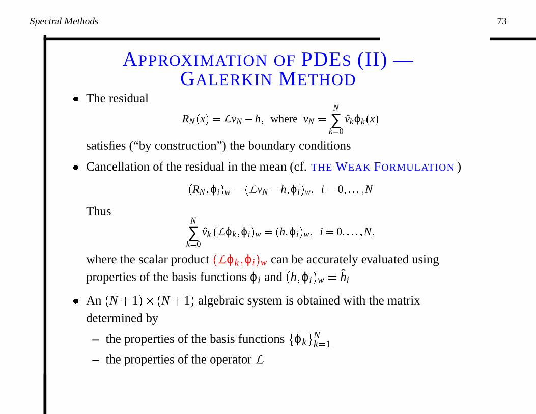
APPROXIMATION OF PDES (II) —GALERKIN METHOD

� The residual

RN � x � LvN� h� where vN

N

∑k� 0

vkϕk � x �

satisfies (“by construction”) the boundary conditions

� Cancellation of the residual in the mean (cf. THE WEAK FORMULATION )� RN� ϕi � w � LvN� h� ϕi � w� i 0� � � � � N

ThusN

∑k� 0

vk � Lϕk� ϕi � w � h� ϕi � w� i 0� � � � � N�

where the scalar product � Lϕk � ϕi � w can be accurately evaluated using

properties of the basis functions ϕi and � h � ϕi � w � hi

� An � N 1 ��� � N 1 � algebraic system is obtained with the matrix

determined by

– the properties of the basis functions � ϕk �

Nk� 1

– the properties of the operator L

Spectral Methods 74

APPROXIMATION OF PDES (III) —COLLOCATION METHOD

� The residual (corresponding to the original inhomogeneous problem)

RN � x � LuN� f� where uN

N

∑k� 0

ukϕk � x �

� Pointwise cancellation of the residual, including the boundary nodes:

���� ��

�

LuN �

xi �� f

�

xi �

i� 1 � � � � � N � 1

B � uN �

x0 �� g �

B � uN �

xN �� g � �

This results in an � N 1 ��� � N 1 � algebraic system. Note that depending

on the properties of the basis � ϕ0 ��� � � � ϕN � , this system may be singular.

� Sometimes an alternative formulation is useful, where the nodal valuesuN � x j � j � 0 ��� � � � N, rather than the expansion coefficients uk, k � 0 ��� � � � Nare unknown. The advantage is a convenient form of the expression for thederivative

u �

p

�

N � xi �

N

∑j� 0

d �

p

�

i j uN � x j ��

where d �

p

� is a p–TH ORDER DIFFERENTIATION MATRIX .

Spectral Methods 75

ORTHONORMAL SYSTEMS (I) —CONSTRUCTION

� THEOREM — Let H be a separable Hilbert space and T a compact

Hermitian operator. Then, there exists a sequence � λn � n �� and � Wn � n ��

such that

1. λn � � ,

2. the family � Wn � n �� forms A COMPLETE BASIS in H

3. T Wn � λnWn for all n � �

� Systems of orthogonal functions are therefore related to spectra of certain

operators, hence the name SPECTRAL METHODS

Spectral Methods 76

ORTHONORMAL SYSTEMS (II) —EXAMPLE # 1

� Let T : L2 � 0 � π � � L2 � 0 � π � be defined for all f � L2 � 0 � π � by T f � u, whereu is the solution of the Dirichlet problem

� u� � f

u � 0 � u � π � 0

Compactness of T follows from the Lax–Milgram lemma and compact

embeddedness of H1 � 0 � π � in L2 � 0 � π � .

� EIGENVALUES AND EIGENVECTORS

λk

1k2 and Wk � 2sin � kx � for k � 1

� Thus, each function u � L2 � 0 � π � can be represented as

u � x � � 2 ∑k � 1

ukWk � x � �where uk � � u � Wk � L2

� � 2π �

π0 u � x � sin � kx � dx .

� Uniform (pointwise) convergence is not guaranteed (only in L2 sense)!

Spectral Methods 77

ORTHONORMAL SYSTEMS (III) —EXAMPLE # 2

� Let T : L2 � 0 � π � � L2 � 0 � π � be defined for all f � L2 � 0 � π � by T f � u, whereu is the solution of the Neumann problem

� u� �� u f

u� � 0 � u� � π � 0

Compactness of T follows from the Lax–Milgram lemma and compact

embeddedness of H1 � 0 � π � in L2 � 0 � π � .

� EIGENVALUES AND EIGENVECTORS

λk

11 � k2 and W0 � x � 1� Wk � 2cos � kx � for k � 1

� Thus, each function u � L2 � 0 � π � can be represented as

u � x � � 2 ∑k � 0

ukWk � x � �where uk � � u � Wk � L2

� � 2π �

π0 u � x � cos � kx � dx .

� Uniform (pointwise) convergence is not guaranteed (only in L2 sense)!

Spectral Methods 78

ORTHONORMAL SYSTEMS (IV) —EXAMPLE # 3

� Expansion in SINE SERIES good for functions vanishing on the boundaries

� Expansion in COSINE SERIES good for functions with first derivatives

vanishing on the boundaries

� Combining sine and cosine expansions we obtain the FOURIER SERIES

EXPANSION with the basis functions (in L2 �� π � π � )Wk � x � eikx� for k � 0

Wk form a Hilbert basis with better properties then sine or cosine series alone.

� FOURIER SERIES vs. FOURIER TRANSFORM —

– FOURIER TRANSFORM : F1 : L2 � � � � L2 � � � ,

F1 � u � � k �

∞

� ∞e

� ikxu � x � dx� k � �

– FOURIER SERIES : F2 : L2 � 0 � 2π � � l2, (i.e., bounded to discrete)

uk F2 � u � � k �

2π

0e

� ikxu � x � dx� k 0� 1� 2� � � �

Spectral Methods 79

ORTHONORMAL SYSTEMS (V) —POLYNOMIAL APPROXIMATION

� WEIERSTRASS APPROXIMATION THEOREM — To any function f � x � that

is continuous in � a � b � and to any real number ε � 0 there corresponds a

polynomial P � x � such that � P � x �� f � x � � C

�

a � b ��� ε, i.e. the set of

polynomials is DENSE in the Banach space C � a � b �

(C � a � b � is the Banach space with the norm � f � C

�

a � b �

� maxx � � a � b ��� f � x ��

� Thus the power functions xk, k � 0 � 1 ��� � � represent a natural basis in C � a � b �

� QUESTION — Is this set of basis functions useful?

NO! — SEE BELOW

Spectral Methods 80

ORTHONORMAL SYSTEMS (VI) —EXAMPLE

� Find the polynomial PN (of order N) that best approximates a functionf � L2 � a � b � [note that we will need the structure of a Hilbert space, hencewe go to L2 � a � b � , but C � a � b ��� L2 � a � b � ], i.e.

b

a

� f � x �� PN � x � �

2 dx �

b

a

� f � x �� PN � x � �

2 dx

where PN � x � a0 � a1x � a2x2

� � � � � aN xN

� Using the formula ∑Nj� 0 a j � e j � ek � � � f � ek � � j � 0 ��� � � � N, where ek � xk

N

∑k� 0

ak

b

axk � j dx

b

ax j f � x � dx

N

∑k� 0

akbk � j � 1� ak � j � 1

k � j � 1

b

ax j f � x � dx

� The resulting algebraic problem is extremely ILL–CONDITIONED , e.g. fora � 0 and b � 1

� A � k j

1k � j � 1

Spectral Methods 81

ORTHONORMAL SYSTEMS (VII) —POLYNOMIAL APPROXIMATION

� Much better behaved approximation problems are obtained with the use of

ORTHOGONAL BASIS FUNCTIONS

� Such systems of orthogonal basis functions are derived by applying the

SCHMIDT ORTHOGONALIZATION PROCEDURE to the system � 1 � x ��� � � � xN

�

� Various families of ORTHOGONAL POLYNOMIALS are obtained depending

on the choice of:

– the domain � a � b � over which the polynomials are defined, and

– the weight w characterizing the inner product ��� � � � w used for

orthogonalization

Spectral Methods 82

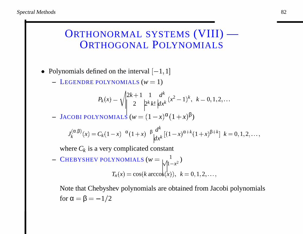
ORTHONORMAL SYSTEMS (VIII) —ORTHOGONAL POLYNOMIALS

� Polynomials defined on the interval �� 1 � 1 �

– LEGENDRE POLYNOMIALS (w � 1)

Pk � x � 2k � 1

21

2k k!dk

dxk � x2� 1 � k� k 0� 1� 2��� � �

– JACOBI POLYNOMIALS (w � � 1� x � α � 1 x � β)

J �

α � β �

k � x � Ck � 1� x �� α � 1 � x �� β dk

dxk � � 1� x � α � k � 1 � x � β � k

� k 0� 1� 2� � � � �

where Ck is a very complicated constant

– CHEBYSHEV POLYNOMIALS (w � 1� 1 � x2 )

Tn � x � cos � k arccos � x � � � k 0� 1� 2� � � � �

Note that Chebyshev polynomials are obtained from Jacobi polynomials

for α � β � � 1

�

2

Spectral Methods 83

ORTHONORMAL SYSTEMS (IX) —ORTHOGONAL POLYNOMIALS

� Polynomials defined on the PERIODIC interval �� π � π �

TRIGONOMETRIC POLYNOMIALS (w � 1)

Sk � x � eikx k 0� 1� 2� � � �

� Polynomials defined on the interval � 0 � ∞ �

LAGUERRE POLYNOMIALS (w � e � x)

Lk � x �

1k!

ex dk

dxk � e

� xxk � � k 0� 1� 2� � � �

� Polynomials defined on the interval �� ∞ � ∞ �HERMITE POLYNOMIALS (w � 1)

Hk � x � �� 1 � k

� 2k k! � π � 1

�

2ex2 dk

dxk e

� x2� k 0� 1� 2� � � �

Spectral Methods 84

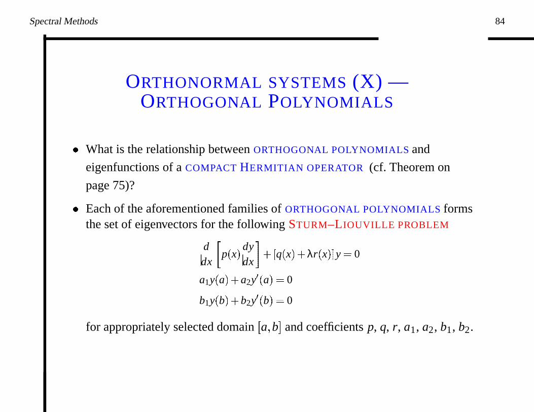
ORTHONORMAL SYSTEMS (X) —ORTHOGONAL POLYNOMIALS

� What is the relationship between ORTHOGONAL POLYNOMIALS and

eigenfunctions of a COMPACT HERMITIAN OPERATOR (cf. Theorem on

page 75)?

� Each of the aforementioned families of ORTHOGONAL POLYNOMIALS formsthe set of eigenvectors for the following STURM–LIOUVILLE PROBLEM

ddx

�

p � x �dydx

�

� � q � x � � λr � x � � y 0

a1y � a � � a2y� � a � 0

b1y � b � � b2y� � b � 0

for appropriately selected domain � a � b � and coefficients p, q, r, a1, a2, b1, b2.

Spectral Methods 85

FOURIER SERIES (I) — CALCULATION OFFOURIER COEFFICIENTS

� TRUNCATED FOURIER SERIES:

uN � x �

N

∑k� � N

ukeikx

� The series involves 2N 1 complex coefficients of the form (weight w � 1):

uk 1

2π

π

� πue

� ikx dx� k � N� � � � � N

� The expansion is redundant for real–valued u — the property of CONJUGATE

SYMMETRY u � k � ¯uk , which reduces the number of complex coefficients to

N 1; furthermore, ℑ � u0 � � 0 for real u, thus one has 2N 1 REAL

coefficients; in the real case one can work with positive frequencies only!

� Equivalent real representation:

uN � x � a0 �

N

∑k� 1

� ak cos � kx � � bk sin � kx � � �where a0 � u0, ak � 2ℜ � uk � and bk � 2ℑ � uk � .

Spectral Methods 86

FOURIER SERIES (II) — UNIFORMCONVERGENCE

� Consider a function u that is continuous, periodic (with the period 2π) and

differentiable; note the following two facts:

– The Fourier coefficients are always less than the average of u

� uk � ��

��

12π

π

� πu � x � eikx dx

��

��

� M � u ��

12π

π

� π

� u � x � � dx

– If v � dαudxα � u �

α� , then uk � vk

�

ik

�

α

� Then, using integration by parts, we have

uk

12π

π

� πu � x � e

� ikx dx 12π

�

u � x �

e � ikx

� ik

�

π

� π

� 12π

π

� πu� � x �

e � ikx

� ikdx

� Repeating integration by parts p times

uk �� 1 � p 12π

π

� πu �

p

� � x �

e � ikx

�� ik � p dx � � uk � �

M � u �

p

� �� k �

p

Therefore, the more regular is the function u, the more rapidly its Fourier

coefficients tend to zero as� n� � ∞

Spectral Methods 87

FOURIER SERIES (III) — UNIFORMCONVERGENCE

� We have

� uk � �

M � u� � �� k �

2

� ∑k �

� ukeikx

� � u0 � ∑n �� 0

M � u� � �

n2

The latter series converges ABSOLUTELY

� Thus, if u is TWICE CONTINUOUSLY DIFFERENTIABLE and its first

derivative is CONTINUOUS AND PERIODIC with period 2π, then its Fourier

series uN � PNu CONVERGES UNIFORMLY to u for� N� � ∞

� SPECTRAL CONVERGENCE – if φ � C∞p �� π � π � , then for all α � 0 there

exists a positive constant Cα such that� φk� �Cα

� n � α, i.e., for a function with an

infinite number of smooth derivatives, the Fourier coefficients vanish faster

than algebraically

Spectral Methods 88

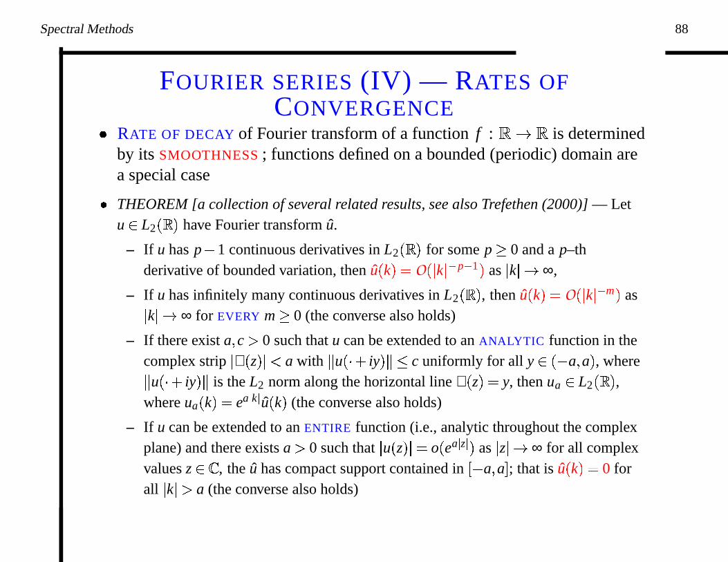
FOURIER SERIES (IV) — RATES OFCONVERGENCE

� RATE OF DECAY of Fourier transform of a function f : � � � is determinedby its SMOOTHNESS ; functions defined on a bounded (periodic) domain area special case

� THEOREM [a collection of several related results, see also Trefethen (2000)] — Letu � L2 � � � have Fourier transform u.

– If u has p� 1 continuous derivatives in L2 � � � for some p � 0 and a p–thderivative of bounded variation, then u � k � O � � k �

� p � 1 � as � k ��� ∞,

– If u has infinitely many continuous derivatives in L2 � � � , then u � k � O � � k �� m � as

� k ��� ∞ for EVERY m � 0 (the converse also holds)

– If there exist a� c � 0 such that u can be extended to an ANALYTIC function in thecomplex strip � ℑ � z � ��� a with � u �� � iy � � � c uniformly for all y � �� a� a � , where

� u �� � iy � � is the L2 norm along the horizontal line ℑ � z � y, then ua � L2 � � � ,where ua � k � ea � k � u � k � (the converse also holds)

– If u can be extended to an ENTIRE function (i.e., analytic throughout the complexplane) and there exists a � 0 such that � u � z � � o � ea � z � � as � z �� ∞ for all complexvalues z �� , the u has compact support contained in �

� a� a � ; that is u � k � 0 forall � k � � a (the converse also holds)

Spectral Methods 89

FOURIER SERIES (V) — RADII OFCONVERGENCE

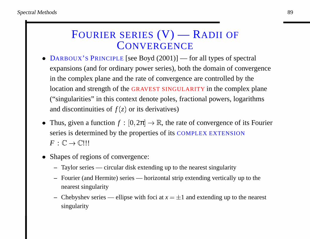
� DARBOUX’S PRINCIPLE [see Boyd (2001)] — for all types of spectral

expansions (and for ordinary power series), both the domain of convergence

in the complex plane and the rate of convergence are controlled by the

location and strength of the GRAVEST SINGULARITY in the complex plane

(“singularities” in this context denote poles, fractional powers, logarithms

and discontinuities of f � z � or its derivatives)

� Thus, given a function f : � 0 � 2π � � � , the rate of convergence of its Fourier

series is determined by the properties of its COMPLEX EXTENSION

F : � � � !!!

� Shapes of regions of convergence:

– Taylor series — circular disk extending up to the nearest singularity

– Fourier (and Hermite) series — horizontal strip extending vertically up to thenearest singularity

– Chebyshev series — ellipse with foci at x � 1 and extending up to the nearestsingularity

Spectral Methods 90

FOURIER SERIES (VI) —PERIODIC SOBOLEV SPACES

� Let Hrp � I � be a PERIODIC SOBOLEV SPACE , i.e.,

Hrp � I � � u : u �

α

� � L2 � I � � α 0� � � � � r � �

where I � �� π � π � is a periodic interval. The space C∞p � I � is dense in Hr

p � I �

� The following two norms can be shown to be EQUIVALENT in H rp:

� u � r

�

∑k �

� 1 � k2 � r

� uk �

2

�

1

�

2

� � u � � r

�

r

∑α� 0

Cαr � u �

α

� �

2

�

1

�

2

Note that the first definition is naturally generalized for the case when r is non–integer!

� The PROJECTION OPERATOR PN commutes with the derivative in thedistribution sense:

� PN u � �

α

� ∑

� k �� N

� ik � αukWk PN u �

α

�

Spectral Methods 91

FOURIER SERIES (VII) —APPROXIMATION ERROR ESTIMATES IN Hs

p �

I

�

� Let r� s � � with 0 � s � r; then we have:� u� PN u � s � � 1 � N2 �

s � r2 � u � r� for u � Hr

p � I �

Proof:

� u� PN u �

2s ∑

� k ��� N

� 1 � k2 � s � r � r

� uk �

2 � � 1 � N2 � s � r ∑

� k ��� N

� 1 � k2 � r

� uk �

2

� � 1 � N2 � s � r

� u �

2r

� Thus, accuracy of the approximation PNu is better when u is SMOOTHER ;

more precisely, for u � Hrp � I � , the L2 leading order error is O � N

� r � which

improves when r increases.

Spectral Methods 92

FOURIER SERIES (VIII) —APPROXIMATION ERROR ESTIMATES IN L∞ �

I

�

� First, a useful lemma (SOBOLEV INEQUALITY) — let u � H1p � I � , then there

exists a constant C such that

� u �

2L∞ �

I

�

� C � u � 0 � u � 1

Proof: Suppose u � C∞p � I � ; note the following facts

– u0 is the average of u

– From the mean value theorem: � x0 � I such that u0 � u � x0 �

Let v � x � � u � x �� u0, then

12 � v � x � �

2

x

x0

v � y � v� � y � dy ��

x

x0

� v � y � �2 dy

�

1

�

2

�

x

x0

� v

� � y � �

2 dy

�

1

�

2

� 2π � v � � v� �

� u � x � � � � u0 � � � v � x � � � � u0 � � 2π1

�

2

� v �

1

�

2� v� �

1

�

2 � C � u �

1

�

20 � u �

1

�

21 �

since v� � u� , � v � � � u � and� u0� � � u � .

As C∞p � I � is dense in H1

p � I � , the inequality also holds for any u � H1p � I � .

Spectral Methods 93

FOURIER SERIES (IX) —APPROXIMATION ERROR ESTIMATES IN L∞ �

I

�

� An estimate in the norm L∞ � I � follows immediately from the previouslemma and estimates in the Hs

p � I � norm� u� PN u �

2L∞ �

I

�

� C � 1 � N2 �� r

2 � 1 � N2 �

1 � r2 �

where u � Hrp � I �

� Thus for r � 1

� u� PN u �2L∞ �

I�

O � N12

� r �

� UNIFORM CONVERGENCE for all u � H1p � I �

(Note that u need only to be CONTINUOUS , therefore this result is stronger

than the one given on page 87)

Spectral Methods 94

FOURIER SERIES (X) —SPECTRAL DIFFERENTIATION

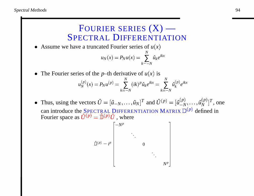
� Assume we have a truncated Fourier series of u � x �

uN � x � PN u � x �

N

∑k� � N

ukeikx

� The Fourier series of the p–th derivative of u � x � is

u �

p�

N � x � PN u �

p

�

N

∑k� � N

� ik � pukeikx

N

∑k� � N

u �

p

�

k eikx

� Thus, using the vectors U � � u � N ��� � � � uN � T and U �

p

� � � u �

p

�

� N ��� � � � u �

p

�

N � T , one

can introduce the SPECTRAL DIFFERENTIATION MATRIX � �

p

� defined inFourier space as U �

p

� � ˆ� �

p

� U , where

ˆ��� p � � ip

� �����������

� N p

. . .

0

. . .

N p�

Spectral Methods 95

FOURIER SERIES (XI) —SPECTRAL DIFFERENTIATION

� Properties of the spectral differentiation matrix in Fourier representation

– � �

p

� is DIAGONAL

– � �

p

� is SINGULAR (diagonal matrix with a zero eigenvalue)

– after desingularization the 2–norm condition number of � �

p

� grows in

proportion to N p (since the matrix is diagonal, this is not an issue)

� QUESTION — how to derive the corresponding spectral differentiation

matrix in REAL REPRESENTATION ?

Will see shortly ...

Spectral Methods 96

SPECTRAL GALERKIN METHOD —NUMERICAL QUADRATURES (I)

� We need to evaluate the expansion (Fourier) coefficients

uk � u� φk � w

b

aw � x � u � x � φk � x � dx� k 0� � � � � N

� QUADRATURE is a method to evaluate such integrals approximately.

� GAUSSIAN QUADRATURE seeks to obtain the best numerical estimate of an

integral �

ba w � x � f � x � dx by picking OPTIMAL POINTS xi, i � 1 ��� � � � N at

which to evaluate the function f � x � .

� THE GAUSS–JACOBI INTEGRATION THEOREM — If the � N 1 �

interpolation points � xi �

Ni� 0 are chosen to be the zeros of PN 1 � x � , where

PN 1 � x � is the polynomial of degree � N 1 � of the set of polynomials whichare orthogonal on � a � b � with respect to the weight function w � x � , then thequadrature formula

b

aw � x � f � x � dx

N

∑i� 0

wi f � xi �is EXACT for all f � x � which are polynomials of at most degree � 2N 1 �

Spectral Methods 97

SPECTRAL GALERKIN METHOD —NUMERICAL QUADRATURES (II)

� DEFINITION — Let K be a non-empty, Lipschitz, compact subset of � d . Let

lq � 1 be an integer. A quadrature on K with lq points consists of:

– A set of lq real numbers � ω1 ��� � � � ωlq � called QUADRATURE WEIGHTS

– A set of lq points � ξ1 ��� � � � ξlq � in K called GAUSS POINTS or

QUADRATURE NODES

The largest integer k such that � p � Pk, � K p � x � dx � ∑lql� 1 ωl p � ξl � is called

the quadrature order and is denoted by kq

� REMARK — As regards 1D bounded intervals, the most frequently used

quadratures are based on Legendre polynomials which are defined on the

interval � 0 � 1 � as Ek � t � � 1k!

dk

dtk � t2� t � k, k � 0. Note that they are orthogonal

on � 0 � 1 � with the weight W � 1.

Spectral Methods 98

SPECTRAL GALERKIN METHOD —NUMERICAL QUADRATURES (III)

� Theorem — Let lq � 1, denote by ξ1 ��� � � � ξlq the lq roots of the Legendre

polynomial Elq � x � and set ωl � �

10 ∏

lqj� 1j �� l

t � ξ j

ξl � ξ jdt. Then

� ξ1 ��� � � � ξlq � ω1 ��� � � � ωlq � is a quadrature of order kq � 2lq� 1 on � 0 � 1 �

Proof — Let � L1 � dots � Llq � be the set of Lagrange polynomials associated

with the Gauß points � ξ1 ��� � � � ξlq � . Then ωl � �

10 Ll � t � dt, 1 � l � lq

– when p � x � is a polynomial of degree less than lq, we integrate both sides

of the identity p � t � � ∑lql� 1 p � ξl � Ll � t � dx, � t � � 0 � 1 � and deduce that the

quadrature is exact for p � x �

– when the polynomial p � x � has degree less than 2lq we write it in the formp � x � � q � x � Elq � x � r � x � , where both q � x � and r � x � are polynomials ofdegree less than lq; owing to orthogonality of the Legendre polynomials,we conclude

1

0p � t � dt

1

0r � t � dt

lq

∑l� 1

ωlr � ξl � lq

∑l� 1

ωl p � ξl � �

since the points ξl are also roots of Elq

Spectral Methods 99

SPECTRAL GALERKIN METHOD —NUMERICAL QUADRATURES (IV)

� PERIODIC GAUSSIAN QUADRATURE — If the interval � a � b � � � 0 � 2π � is

periodic, the weight w � x � � 1 and PN � x � is the trigonometric polynomial of

degree N, the Gaussian quadrature is equivalent to the TRAPEZOIDAL RULE

(i.e., the quadrature with unit weights and equispaced nodes)

� Evaluation of the spectral coefficients:

– Assume � φ �

Nk� 1 is a set of basis functions orthogonal under the weight w

uk

b

aw � x � u � x � φk � x � dx � �

N

∑i� 0

w � xi � u � xi � φk � xi � � k 0� � � � � N�

where xi are chosen so that φN 1 � xi � � 0, i � 0 ��� � � � N– Denoting U � � u0 ��� � � � uN � T and U � � u � x0 � ��� � � � u � xN � � T we can write the

above as

U � � U �

where � is a TRANSFORMATION MATRIX

Spectral Methods 100

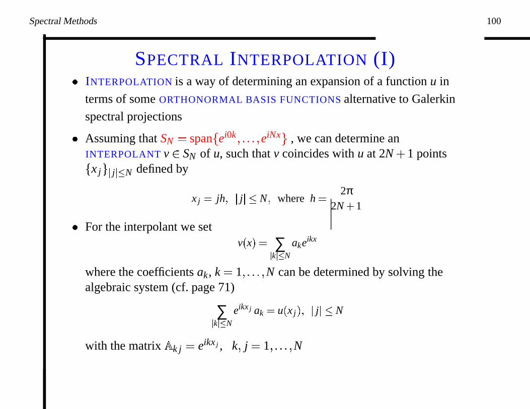
SPECTRAL INTERPOLATION (I)� INTERPOLATION is a way of determining an expansion of a function u in

terms of some ORTHONORMAL BASIS FUNCTIONS alternative to Galerkin

spectral projections

� Assuming that SN � span � ei0k ��� � � � eiNx

� , we can determine anINTERPOLANT v � SN of u, such that v coincides with u at 2N 1 points

� x j � � j �� N defined by

x j jh� � j � � N� where h 2π2N � 1

� For the interpolant we setv � x � ∑

� k �� N

akeikx

where the coefficients ak, k � 1 ��� � � � N can be determined by solving thealgebraic system (cf. page 71)

∑

� k �� N

eikx j ak u � x j � � � j � � N

with the matrix � k j � eikx j , k � j � 1 ��� � � � N

Spectral Methods 101

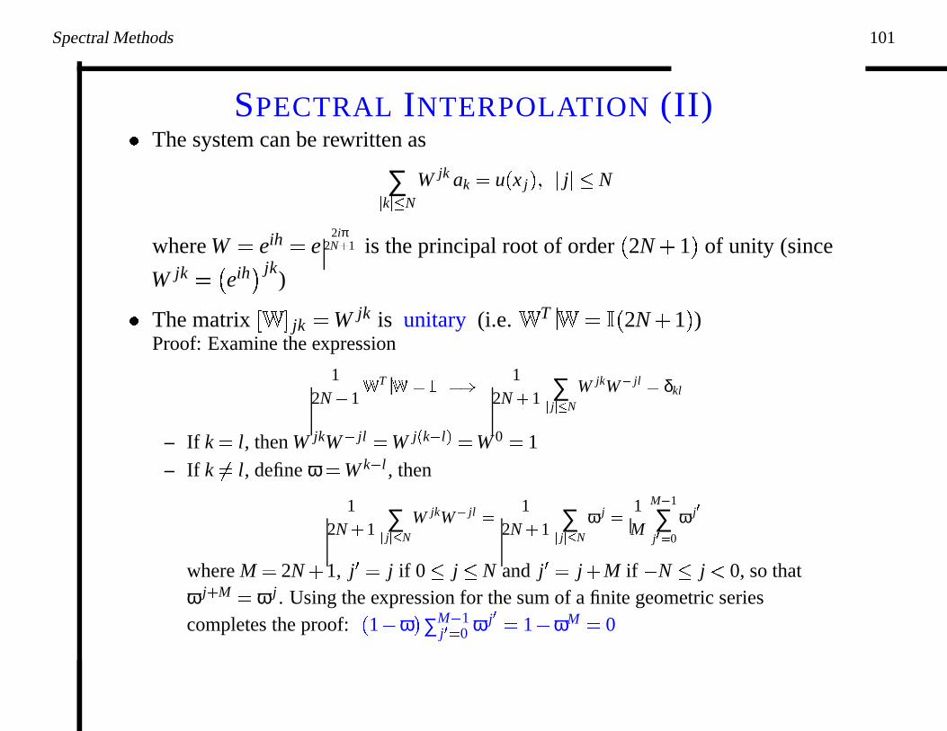
SPECTRAL INTERPOLATION (II)� The system can be rewritten as

∑

� k �� N

W jk ak u � x j � � � j � � N

where W � eih � e2iπ

2N � 1 is the principal root of order � 2N 1 � of unity (since

W jk � � eih

�jk

)

� The matrix ��� � jk � W jk is unitary (i.e. � T � � � � 2N 1 � )Proof: Examine the expression

12N 1

� T� � � � � 12N 1 ∑

� j � N

W jkW

� jl� δkl

– If k l, then W jkW � jl W j

�

k � l� W 0 1

– If k l, define ω W k � l , then

12N 1 ∑

� j � N

W jkW

� jl�

12N 1 ∑

� j � N

ω j�

1M

M � 1

∑j� � 0

ω j�

where M 2N � 1, j� j if 0 � j � N and j� j � M if� N � j� 0, so thatω j � M ω j . Using the expression for the sum of a finite geometric seriescompletes the proof: � 1� ω � ∑M � 1

j� � 0 ω j� 1� ωM 0

Spectral Methods 102

SPECTRAL INTERPOLATION (III)� Since the matrix � is unitary and hence its INVERSE is given by its

TRANSPOSE , the Fourier coefficients of the INTERPOLANT of u in SN can becalculated as follows:

ak

12N � 1 ∑

� k �� N

z jW

� jk� where z j u � x j �

� The mapping

� z j � � j �� N

� � � ak � � k �� N

is referred to as DISCRETE FOURIER TRANSFORM (DFT)

� Straightforward evaluation of the expressions for ak, k � 1 ��� � � � N(matrix–vector products) would result in the computational cost O � N2 � ;clever factorization of this operation, known as the FAST FOURIER

TRANSFORMS (FFT) , reduces this cost down to O � N log � N � �

� See www.fftw.org for one of the best publicly available implementations of

the FFT.

Spectral Methods 103

SPECTRAL INTERPOLATION (IV)� Let PC : C0

p � I � � SN be the mapping which associates with u its interpolantv � SN . Let ��� � � � N be the GAUSSIAN QUADRATURE approximation of theinner product ��� � � �

� u� v �

π

� πuvdx � 1

2N � 1 ∑

� j �� N

u � x j � v � x j �� � u� v � N

� By construction, the operator PC satisfies:

� PCu � � x j � u � x j � � � j � � N

and therefore also (orthogonality of the defect to SN )� u� PCu� vN � N 0��� vN � SN

� By the definition of PN we have

� u� PNu� vN � 0�� vN � SN

� Thus, PCu � x � � ∑Nk� � N � u � eikx � Neikx can be obtained analogously to

PNu � x � � ∑Nk� � N � u � eikx � eikx by replacing the scalar product ��� � � � with the

DISCRETE SCALAR PRODUCT ��� � � � N

Spectral Methods 104

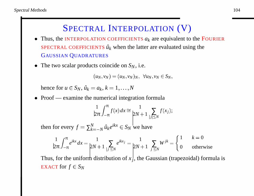
SPECTRAL INTERPOLATION (V)� Thus, the INTERPOLATION COEFFICIENTS ak are equivalent to the FOURIER

SPECTRAL COEFFICIENTS uk when the latter are evaluated using the

GAUSSIAN QUADRATURES

� The two scalar products coincide on SN , i.e.

� uN� vN � � uN� vN � N�� uN� vN � SN�

hence for u � SN , uk � ak, k � 1 ��� � � � N

� Proof — examine the numerical integration formula

12π

π� π

f � x � dx � 12N � 1 ∑

� j �� N

f � x j � ;

then for every f � ∑Nk� � N ukeikx � SN we have

12π

π

� πeikx dx 1

2N � 1 ∑

� j �� N

eikx j 12N � 1 ∑

� j �� N

W jk

1 k 0

0 otherwise

Thus, for the uniform distribution of x j, the Gaussian (trapezoidal) formula is

EXACT for f � SN

Spectral Methods 105

SPECTRAL INTERPOLATION (VI)� Relation between Fourier coefficients uk of a function u � x � and Fourier

coefficients ak of its interpolant; assume that u � x � �� SN

uk

12π

π

� πuW k dx� Wk � x � eikx

ak

12N � 1 ∑

� j �� N

u � x j � Wk � x j �

� THEOREM — For u � C0p � I � we have the relation

ak ∑l �

uk � lM� where M 2N � 1

Proof — Consider the set of basis functions (in L2 � I � ) Uk � eikx. We have:

� Uk� Un � N

12N � 1 ∑

� j �� N

Uk � x j � Un � x j � 1

2N � 1 ∑

� j �� N

W j

�

k � n

�

1 k n � mod M �

0 otherwise

Since PCu � ∑ � j �� N a jWj , we infer from � PCu � Wk � N � � u � Wk � N that

ak � PCu� Wk � N � u� Wk � N �

∑n �

unWn� Wk

� N

∑n �

un

�

Wn� Wk

� N

∑l �

uk � lM

Spectral Methods 106

SPECTRAL INTERPOLATION (VII)� Thus

u � x j � v � x j �

∞

∑k� � ∞

ukeikx j ∑

� k �� N

akeikx j ∑

� k �� N

uk � ∑l � � � 0 �

uk � lM eikx j

� EXTREMELY IMPORTANT COROLLARY CONCERNING INTERPOLATION

— two trigonometric polynomials eik1x and eik2x with different frequencies k1

and k2 are equal at the collocation points x j,� j� � N when

k2� k1 � l � 2N 1 � � l � 0 ��� 1 ��� � � �

Therefore, give a set of values at the collocation points x j,� j� � N, it is

impossible to distinguish between eik1x and eik2x. This phenomenon is

referred to as ALIASING

� Note, however, that the modes appearing in the alias term correspond to

frequencies larger than the cut–off frequency N.

Spectral Methods 107

SPECTRAL INTERPOLATION (VIII) —ERROR ESTIMATES IN Hs

p �

I

�

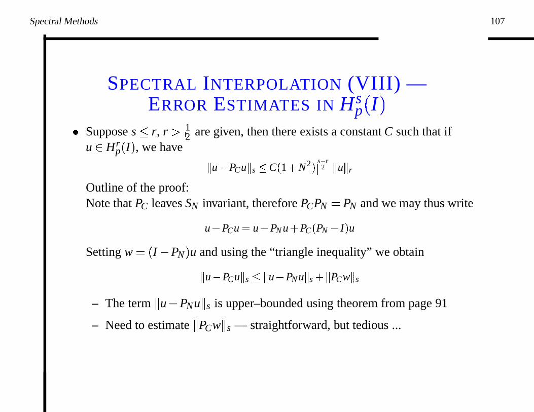
� Suppose s � r, r � 12 are given, then there exists a constant C such that if

u � Hrp � I � , we have

� u� PCu � s � C � 1 � N2 �

s � r2 � u � r

Outline of the proof:Note that PC leaves SN invariant, therefore PCPN � PN and we may thus write

u� PCu u� PN u � PC � PN� I � u

Setting w � � I� PN � u and using the “triangle inequality” we obtain

� u� PCu � s � � u� PN u � s � � PCw � s

– The term � u� PNu � s is upper–bounded using theorem from page 91

– Need to estimate � PCw � s — straightforward, but tedious ...

Spectral Methods 108

SPECTRAL INTERPOLATION (IX)� Until now, we defined the Discrete Fourier Transform for an ODD number

� 2N 1 � of grid points

� FFT algorithms generally require an EVEN number of grid points

� We can define the discrete transform for an EVEN number of grid points byconstructing the interpolant in the space SN for which we havedim � SN � � 2N. To do this we choose:

x j jh� � N � 1 � j � N

h πN

� All results presented before can be established in the case with 2N grid

points with only minor modifications

� However, now the N-th Fourier mode uN does not have its complex

conjugate! This coefficient is usually set to zero (uN � 0) to avoid an

uncompensated imaginary contribution resulting from differentiation

� ODD or EVEN collocation depending on whether M � 2N 1 or M � 2N

Spectral Methods 109

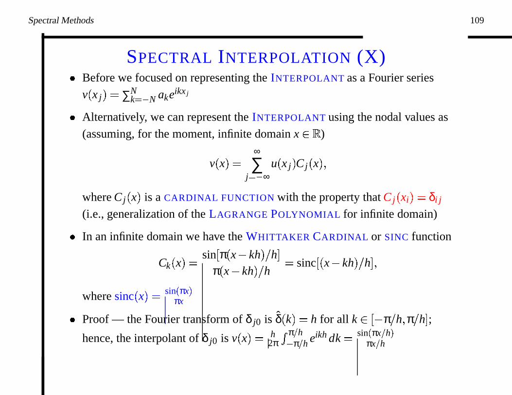
SPECTRAL INTERPOLATION (X)� Before we focused on representing the INTERPOLANT as a Fourier series

v � x j � � ∑Nk� � N akeikx j

� Alternatively, we can represent the INTERPOLANT using the nodal values as

(assuming, for the moment, infinite domain x � � )

v � x � �

∞

∑j� � ∞

u � x j � C j � x � �

where C j � x � is a CARDINAL FUNCTION with the property that C j � xi � � δi j

(i.e., generalization of the LAGRANGE POLYNOMIAL for infinite domain)

� In an infinite domain we have the WHITTAKER CARDINAL or SINC function

Ck � x � � sin � π � x� kh � �h �

π � x� kh � �

h� sinc � � x� kh � �

h � �

where sinc � x � � sin

�

πx

�

πx

� Proof — the Fourier transform of δ j0 is δ � k � � h for all k � �� π

�

h � π �

h � ;hence, the interpolant of δ j0 is v � x � � h

2π �

π

�

h

� π

�

h eikh dk � sin

�

πx

�

h

�

πx

�

h

Spectral Methods 110

SPECTRAL INTERPOLATION (XI)� Thus, the spectral interpolant of a function in an INFINITE domain is a linear

combination of WHITTAKER CARDINAL functions

� In a PERIODIC DOMAIN we still have the representation

v � x � �

N � 1

∑j� 0

u � x j � S j � x � �

but now the CARDINAL FUNCTIONS have the form

S j � x � � 1N

sin

�

N � x� x j �

2

�

cot

�

� x� x j �

2

�

� Proof — similar to the previous (unbounded) case, except that now the

interpolant in given by a DISCRETE Fourier Transform

� The relationship between the Cardinal Functions corresponding to the

PERIODIC and UNBOUNDED domains

S0 � x � � 12N

sin � Nx � cot � x �

2 � �

∞

∑m� � ∞

sincx� 2πm

h

Spectral Methods 111

SPECTRAL DIFFERENTIATION (I)� Two ways to calculate the derivative w � x j � � u� � x j � based on the values

u � x j � , where 0 � j � 2N 1; denote U � � u0 ��� � � � u2N 1 � T and

U� � � u� 0 ��� � � � u� 2N 1 � T

� METHOD ONE — approach based on differentiation in Fourier space:

– calculate the vector of Fourier coefficients U � � U

– apply the diagonal differentiation matrix U� � ˆ� U (cf. page 94)

– return to real space via inverse Fourier transform U � �

T U

� REMARK — formally we can write

U� � �

T ˆ� � U �

however in practice matrix operations are replaced by FFTs

Spectral Methods 112

SPECTRAL DIFFERENTIATION (II)� METHOD TWO — approach based on differentiation (in real space) of the

interpolant u� � x j � � v� � x j � � ∑N � 1j� 0 u � x j � S� j � x � , where the cardinal function

has the following derivatives

S� � x j �

��

�

0� j 0 � mod N �

12 �� 1 � j cot � jh

�

2 � � j 0 � mod N �

� Thus, since the interpolant is a linear combination of shited CardinamFunctions, the differentiation matrix has the form of a TOEPLITZCIRCULANT matrix

� �

��

��

��

��

��

��

��

��

��

��

��

�

0 � 12 cot �� 1h � 2

� 12 cot �� 1h � 2

...

... 1

2 cot �� 2h � 2

12 cot �� 2h � 2

... � 1

2 cot �� 3h � 2

� 12 cot �� 3h � 2

...

.

.

.

.

.

.

...

... 1

2 cot �� 1h � 2

12 cot �� 1h � 2 0

��

��

��

��

��

��

��

��

��

��

��

� Higher–order derivatives obtained calculating S �

p

� � x j �