Page 1
Spectral modeling of time series with missing data
Paulo C. Rodrigues1 and Miguel de Carvalho1,2
1Center for Mathematics and Applications, Faculty of Sciences and Technology,
Nova University of Lisbon, 2829-516 Caparica, Portugal
2Swiss Federal Institute of Technology, Ecole Polytechnique Federale de Lausanne,
CH-1015 Lausanne, Switzerland
E-mail: [email protected] and [email protected]
Abstract
Singular spectrum analysis is a natural generalization of principal component methods for time series
data. In this paper we propose an imputation method to be used with singular spectrum-based tech-
niques which is based on a weighted combination of the forecasts and hindcasts yield by the recurrent
forecast method. Despite its ease of implementation, the obtained results suggest an overall good fit of
our method, being able to yield a similar adjustment ability in comparison with the alternative method,
according to some measures of predictive performance.
AMS Subject Classification: 37M10; 62H25
Key Words: Karhunen–Loeve decomposition; missing data; singular spectrum analysis; time series
analysis
1
Page 2
1 Introduction
Principal component analysis is one of the main tools in multivariate data analysis. The original context
under which these methods were developed, makes it however inappropriate for the analysis of time
series, but an increasingly popular technique—known as singular spectrum analysis—is often considered
as the natural extension of principal component methods for dependent data. The core idea of singular
spectrum analysis lies in the decomposition of the series of interest into several building blocks that can be
classified as trends, oscillatory, or noise components; some algorithms based on such decomposition have
been proposed to conduct out-of-sample forecasts, and the recurrent forecast algorithm is one of the most
used in applications (Golyandina et al., 2001, §2). Singular spectrum-based techniques find their original
motivation in the classical Karhunen–Loeve decomposition (Loeve, 1978) and other classical results on
the orthogonal representation of continuous stochastic processes. Even though there is some lack of
consensus over the literature, a broad share of the roots of these spectral methods is generally attributed
to the works of Basilevsky and Hum (1979) and of Broomhead and King (1986). Known applications
include meteorology (Paegle et al., 2000), climatology (Allen and Smith, 1996), geophysics (Kondrashov
and Ghil, 2006), forecasting (Hassani et al., 2009), econometrics (de Carvalho et al., 2012), among many
others.
In this paper we propose a missing value imputation method to be used with singular spectrum-based
techniques. Our method is based on a suitable convex linear combination of forecasts and hindcasts
yielded by the recurrent forecast algorithm—hence replacing the problem of imputation by one of fore-
casting. We apply our method to a classical data set, depicted in Figure 1, which contains information
on the total volume of passengers in a group of international airline firms (Brown, 1963; Box et al., 2008).
These data were also considered by Golyandina and Osipov (2007), allowing us to perform direct com-
parisons with the procedure proposed in the said paper, and to assess the performance of our method in
comparison with the competing one. The obtained results suggest an overall good fit of our method and
that even though conceptually simple, it is able to fit with an accuracy similar to the alternative method,
according to some measures of predictive performance. The scope of application of our method goes be-
yond the domain of singular spectrum-based techniques—by reducing in general a time series imputation
problem into one of a forecast nature—, but since our main interest is on such spectral methods we do
not address such extensions here. It should be pointed out, however, that with the due modifications
our procedure can be used in conjunction with alternative forecast algorithms, to handle missing data
problems in time series analysis.
2
Page 3
0
100
200
300
400
500
600
700
1949 1951 1953 1955 1957 1959 1961
Num
ber o
f pas
seng
ers
(in
thou
sand
s)
Time (in years)
Figure 1: Monthly traffic of passengers in a group of several international airline firms (Brown, 1963; Box et al., 2008).
This paper is organized as follows. In the next section we give an overview of the modus operandi
of singular spectrum-based techniques. In §3 we introduce our recurrent imputation method (RIM) and
give an illustration in §4. The paper closes in §5 where some final remarks are given.
2 An overview of singular spectrum-based techniques
2.1 Prefatory decomposition theory
To lay groundwork on singular spectrum-based techniques, here we set forth some preliminary results
on the orthogonal representation of stochastic processes. These results provide the theoretical underpin-
ning which underlies the basic motivation behind these spectral methods. One of the most well-known
orthogonal representations of a stochastic process is the Karhunen–Loeve decomposition (Loeve, 1978),
which is stated in Lemma 1 below. Roughly speaking this decomposition guarantees that any random
variable which is continuous in quadratic mean can be represented as a linear combination of orthogonal
functions. A corresponding result for the autocovariance function—the so-called Mercer’s theorem—also
holds and states that under some regularity conditions, the autocovariance g(r, s) can be written as
g(r, s) =
∞∑i=1
√λiωi(r)ωi(s), (1)
where ωi(r) denotes the orthonormalized eigenfunctions of the autocovariance function g(r, s), and the
λi denote the corresponding eigenvalues; a proof of this classical result can be found for instance in
3
Page 4
Hochstadt (1989, p. 90). The decomposition accomplished by Mercer’s theorem can then be employed to
offer an orthogonal representation of the stochastic process itself, rather than the autocovariance function.
Decomposition (1) is at the crux of the establishment of the proper orthogonal decomposition theorem;
the proof of this result can be found elsewhere (Loeve, 1978, pp. 144–145).
Lemma 1. A random function Y (t) which is continuous in quadratic mean on a closed interval I = [0, t]
admits on I an orthogonal decomposition of the form
Y (t) =
∞∑i=1
√λiωi(t)νi, (2)
for some stochastic orthogonal quantities νi, iff λi and ωi(t) respectively denote the eigenvalues and the
orthonormalized eigenfunctions of the autocovariance function g(r, s).
Despite the broadness of this theoretical result, in practice a discrete variant of decomposition (2) is often
preferred to conduct multivariate data analysis. Hence, instead of considering the eigenfunctions one uses
instead the eigenvectors of a discrete version of the autocovariance function g(r, s). Additionally, from a
practical stance, we are often confined to the truncation of a finite number of terms in the decomposition
(2), and the name of this decomposition is at the origin of the alternative naming of principal component
analysis as ‘Karhunen–Loeve transformation’, and alike.
2.2 Modus operandi of the method
The crux of the singular spectrum analysis can be dissociated in two phases—decomposition and recon-
struction—, with two steps each.
Embedding: This is the preparatory step of the method. The core concept assigned to this step is given
by the trajectory matrix, i.e., a lagged version of the original series y = ( y1 · · · yn )T. Formally, the
trajectory matrix l × k is defined as
Y =
y1 y2 · · · yκ
y2 y3 · · · yκ+1
......
. . ....
yl yl+1 · · · yl+(κ−1)
, (3)
where κ is such that Y includes all the observations in the original time series, i.e., κ = n− l + 1.
To set terminology we refer to each vector yi =(yi · · · yl+(i−1)
)T, i = 1, . . . , κ, as a window; the
window length l, is a parameter to be defined by the user. Observe that Y is a Hankel matrix, where
4
Page 5
the original series y lies in the junction formed by the first column and the last row; it can also be useful
to think of the trajectory matrix as a sequence of κ windows, i.e., Y = ( y1,l · · · yκ,l ). The trajectory
matrix also finds application in the estimation of the lag-covariance matrix Σ of the source series y. In
effect, Broomhead and King (1986) proposed the following estimate
ΣBK =1
lYTY.
As an alternative, one can also rely the estimate of the lag-covariance matrix using the proposal of
Vautard and Ghil (1989), which is given by
ΣV G =
1
n− |i− j|
n−|i−j|∑t=1
ytyt−|i−j|
l×l
.
Observe that this estimate yields a Toeplitz matrix, i.e., a diagonal-constant matrix.
Singular Value Decomposition: In the second step we perform a singular value decomposition (SVD)
of the trajectory matrix. Hence, from a eigenanalysis of the matrix YYT we collect the eigenvalues
λ1 ≥ · · · ≥ λd, where d = rank(YYT) and the corresponding left and right singular vectors which we
respectively denote by wi and vi. Thus, we are able to rewrite the trajectory matrix as
Y =
d∑i=1
√λiwiv
T
i .
We now turn to the second phase of the method—reconstruction. This includes the steps of grouping
and diagonal averaging.
Grouping: In the grouping step, the selection of the m principal components takes place. Formally, let
I = {1, . . . ,m} and Ic = {m + 1, . . . , d}. The point here is to choose the first m leading eigentriples
associated to the signal and exclude the remaining (d−m) associated to the noise. Stated differently, at
this step we search for a ‘suitable’ selection of the set I, which allows us to disentangle the series Y into
Y =∑i∈I
√λiwiv
T
i + ε,
where ε denotes an error term, and the remainder summands represents the signal. In practice, this is
typically done through readjusted methods for selecting a reasonable number of principal components m.
Diagonal Averaging: The central idea in this step is the reconstruction of the deterministic component
of the series—the signal. A natural way to do this is to transfigure the matrix Y − ε obtained in the
5
Page 6
previous step into an Hankel matrix. The point here is to reverse the process done so far, returning
to a reconstructed variant of the trajectory matrix (3), and thus the signal component of the series.
An optimal way to do this is to average over all the elements of the several antidiagonals. Formally,
consider the linear space Ml,κ formed by the collection of all the l × κ matrices, and let {hl}nl=1 denote
the canonical basis of Rn. Further, consider the matrix X = [xi,j ] ∈ Ml×κ. The diagonal averaging
procedure is hence carried on by the mapping D :Ml×κ → Rn defined as
D(X) =
κ+l∑w=2
hw−1∑
(i,j)∈Aw
xi,j|Aw|
.
Here | · | stands for the cardinal operator, and
Aw = {(i, j) : i+ j = w}, i = 1, . . . , l, j = 1, . . . , κ.
Hence we are now able to write the signal component of the series through the diagonal averaging
procedure described above
y = D
(∑i∈I
√λiwiv
T
i
).
Here and below, the tildes will be used to denote reconstruction.
3 Recurrent singular spectrum-based procedures
3.1 Recurrent forecast method
We now address the issue of using singular spectrum-based techniques to conduct out-of-sample forecasts.
The method presented below is often referred in the literature as the recurrent forecast algorithm, and
plays an important role in singular spectrum-based forecasting theory and practice; alternative forecast
methods can be found elsewhere (Golyandina et al., 2001, §2). Essentially, the method relies on the
presumption that we are able to write the ith observation yi as a linear combination of the preceding
(l − 1) observations. Put differently, we consider that the following linear recurrent formula holds
yi = a1yi−1 + · · ·+ al−1yi−(l−1), i ≥ l,
for a suitable choice of the coefficients a = ( a1 · · · al−1 )T. We are then faced with the question: What
coefficients should we use in this linear recurrent formula? To answer this question, consider the matrix
constituted by the eigenvectors of YYT suitably subdivided as follows
6
Page 7
W =
U1 | U2
−−− | − −−
u1 | u2
.
The matrix U1 includes the first (l − 1) components of the eigenvectors associated to the signal, and u1
contains the last components of those eigenvectors. The matrices U2 and u2 are analogously defined but
are correspondent to the remainder (d−m) components associated to the noise. Essentially, the question
introduced above concerns a particular case of the problem of the recovery of a vector component in a
subspace. Hence, using Proposition 1 in Golyandina and Osipov (2007), it can be shown that
a =M [U1 � (u1 ⊗ 1l−1)] 1m
1− ‖u1‖2, (4)
where ‖ · ‖ denotes the Euclidean norm, � and ⊗ respectively denote the componentwise Hadamard and
the tensor Kronecker products, and
M =
0 0 · · · 0 1
0 0 · · · 1 0
......
. . ....
...
0 1 · · · 0 0
1 0 · · · 0 0
. (5)
The coefficients a are frequently written in the literature in a different notation, but we show in the
appendix that our form of writing the forecast coefficients (4), is tantamount to such representations.
The 1-step-ahead out-of-sample forecast proposed by the method is then given by the following linear
combination of the last (l − 1) reconstructed values of the series
−→y n+1 =
l−1∑i=1
aiyn−i,
where the coefficients a are given as in (4). In general we have that for further steps-ahead, the out-of-
sample forecasts are given by
−→y n+2 = a1−→y n+1 +
l−1∑i=2
aiyn−i
...
−→y n+(l−1) =
l−1∑i=1
ai−→y n−i.
for 2, . . . , (l− 1) steps-ahead, respectively. In the latter equations and in the remainder of this paper the
notation ‘−→y ’ is used to denote forecasts.
7
Page 8
3.2 Recurrent imputation method
We now concern ourselves with the problem of imputation of missing values on a determined time series
of interest. Specifically, we propose a method to which we refer as the recurrent imputation method
(RIM), to be applied to a series y = ( y1 · · · yn )T
with a block of k sequential missing values. Without
loss of generality, consider the following decomposition of the series of interest
y =
y1,m
ym+1,k
ym+k+1,m?
, (6)
where m? = n−m− k, and
yi,l =(yi · · · yl+(i−1)
)Tdenotes the window of length l starting on the ith observation. The decomposition given in (6) breaks
the series into several pieces of interest, namely: the first block of m observations, given by y1,m; the
block of k missing observations, denoted by ym+1,k; the second block of m? observations, stockpiled in
ym+k+1,m? . Observe further that this structure is sufficiently rich to include the case wherein the missing
data do not occur in a sequential block. This observation is consequential for obvious generalizations of
the method described below.
The estimation object of interest below is the block of k missing values, ym+1,k, and thus our interest
is in obtaining a series
y =
y1,m
ym+1,k
ym+k+1,m?
. (7)
For such purpose, we propose a method based in a suitable weighted average of the forecasts and hindcasts
of the recurrent forecast method; these are formally defined as
−→ym+1,k =(−→y m+1 · · · −→y m+k
)T
, ←−ym+1,k =(←−y m+1 · · · ←−y m+k
)T
, (8)
respectively. In the expressions comprised in (8), and in the remainder of this paper, “←−y ” will be used to
denote hindcasts. Put differently, “←−y ” will be used to represent the forecasts of a new series in reverse
order, i.e., a reordered series wherein the temporal axis is reversed. Thus, for instance, the second block
of the series in reverse order is given by yT
m+k+1,m?M, with M defined according to (5); an illustration of
the linkage between the second block of the series in direct and inverse order is presented in Figure 2. To
8
Page 9
be precise, the matrix M to which we refer in this section consists of a variant of the matrix introduced
in (5) with size m? ×m?.
As mentioned above, the recurrent imputation method intends to establish an equilibrium between the
forecasts and hindcasts achieved by the recurrent forecast algorithm. Specifically, our method employs
the following estimate for the block of k missing values
ym+1,k = θ �−→ym+1,k + (1k − θ)←−ym+1,k, (9)
where � denotes the componentwise Hadamard product and
θ = ( θ1 · · · θk )T,
denotes a set of weights to assign to the forecasts yielded by the recurrent forecast algorithm.
To shed some light on the mechanics of our method, suppose that we have a series of length 20,
with a block of 3 sequential missing values, starting at the 8th observation. For the sake of illustration,
suppose that we consider a weighting scheme such that θ1 = 3/4, θ2 = 1/2 and θ3 = 1/4. The first step
towards the implementation of the recurrent imputation method passes through the application of the
recurrent forecast algorithm for yielding 3 values, based on the first 7 observations. Moreover, to obtain
the hindcasts, one should place the last 10 observations in inverse order and forecast over that series.
Finally, the execution of our method is complete after computing a convex linear combination of the
forecasts previously obtained according to (9). Thus, and according with the weighting scheme defined
above, for the first imputed value, the forecast would contribute with 75%, being the remainder due to
the hindcast. The remaining imputed values would be computed though a similar procedure.
In what concerns practical implementation of the method, the parameter θ can be calibrated using the
first block, y1,m, and the second block, ym+k+1,n−m−k, as training sets with the objective of optimizing
some criteria of interest, say minimization of the mean squared error, or by placing a prior structure over
θ. Alternatively, one can also define an a priori structure for θ. Note further that we can also obtain an
alternative representation for the RIM, by introducing (9) in (7) and performing the due simplifications,
i.e.
y =
y1,m
θ(−→ym+1,k −←−ym+1,k
)+←−ym+1,k
ym+k+1,m?
.
9
Page 10
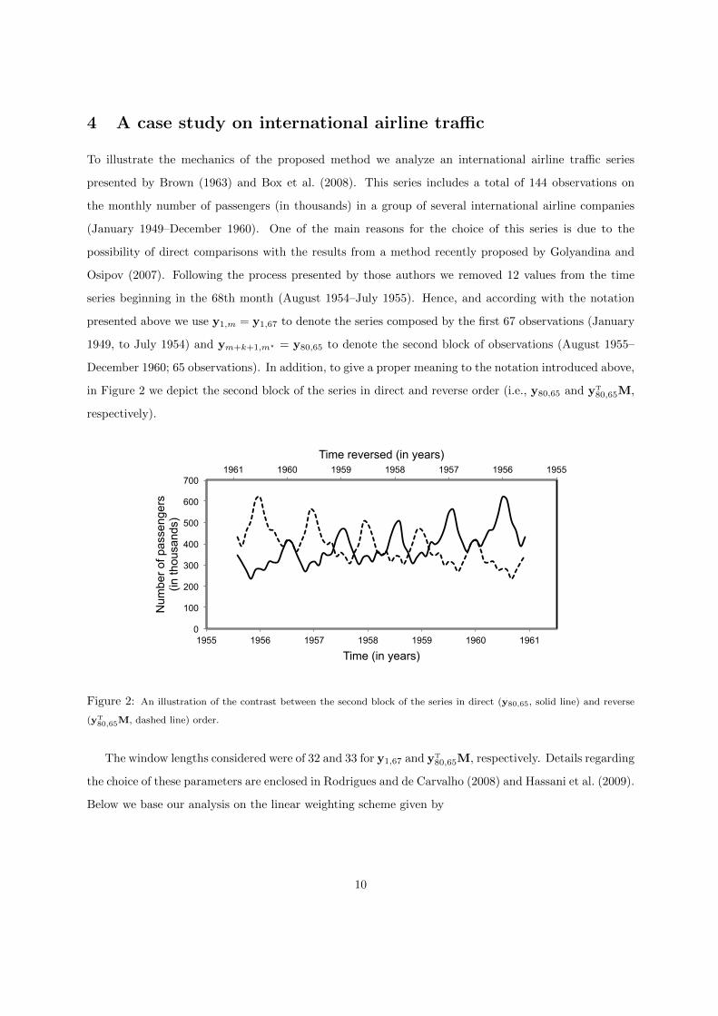
4 A case study on international airline traffic
To illustrate the mechanics of the proposed method we analyze an international airline traffic series
presented by Brown (1963) and Box et al. (2008). This series includes a total of 144 observations on
the monthly number of passengers (in thousands) in a group of several international airline companies
(January 1949–December 1960). One of the main reasons for the choice of this series is due to the
possibility of direct comparisons with the results from a method recently proposed by Golyandina and
Osipov (2007). Following the process presented by those authors we removed 12 values from the time
series beginning in the 68th month (August 1954–July 1955). Hence, and according with the notation
presented above we use y1,m = y1,67 to denote the series composed by the first 67 observations (January
1949, to July 1954) and ym+k+1,m? = y80,65 to denote the second block of observations (August 1955–
December 1960; 65 observations). In addition, to give a proper meaning to the notation introduced above,
in Figure 2 we depict the second block of the series in direct and reverse order (i.e., y80,65 and yT80,65M,
respectively).
1955 1956 1957 1958 1959 1960 1961
0
100
200
300
400
500
600
700
1955 1956 1957 1958 1959 1960 1961
Time reversed (in years)
Num
ber o
f pas
seng
ers
(in
thou
sand
s)
Time (in years)
Figure 2: An illustration of the contrast between the second block of the series in direct (y80,65, solid line) and reverse
(yT80,65M, dashed line) order.
The window lengths considered were of 32 and 33 for y1,67 and yT80,65M, respectively. Details regarding
the choice of these parameters are enclosed in Rodrigues and de Carvalho (2008) and Hassani et al. (2009).
Below we base our analysis on the linear weighting scheme given by
10
Page 11
θi =k + 1− ik + 1
, i = 1, . . . , k,
or alternatively in the vector notation of §3.2 it is given by
θ =(
kk+1 · · · 1
k+1
)T
. (10)
As anticipated above other weight schemes could have been considered, even though this scheme seems
a natural one for data which are equally spaced in time. It can be verified however in Tables 1 and 2
that even with this simple weighting scheme we achieved forecast errors comparable with the ones yield
with the method proposed by Golyandina and Osipov (2007), but with our method yielding a lower
root mean squared error; this suggests that for these data the RIM would be particularly convenient
for a decision-maker with a quadratic loss function. The good performance of our imputation method
can be also noticed in Figure 3 where it is visible a clear proximity between the original series and
the imputed values. We have also tried other methods, such as an interpolated Kalman filter-based
imputation method (Zeileis and Grothendieck, 2005) and an imputation method based on the bootstrap
(Davison and Hinkley, 1997), but the obtained RMSE were much larger than the ones presented in Table
1. In the latter case the problem may be due to a normality assumption on which the bootstrap-based
imputation model relies—and which may fail to hold for these data; see eq. (1) in Honaker et al. (2011).
A fair comparison with these methods would however require an exhaustive simulation study.
11
Page 12
Table 1: An illustration of the recurrent imputation method.
Month Hindcasts Forecasts Weights Imputed Values Original Series
68 323.99 285.74 0.9231 288.68 293
69 303.22 244.40 0.8462 253.45 259
70 274.63 207.26 0.7692 222.81 229
71 254.26 189.38 0.6923 209.34 203
72 286.02 185.40 0.6154 224.10 229
73 291.03 186.41 0.5385 234.69 242
74 281.88 191.88 0.4615 240.34 233
75 309.72 207.88 0.3846 270.55 267
76 297.90 221.03 0.3077 274.25 269
77 290.70 224.84 0.2308 275.50 270
78 332.16 247.90 0.1538 319.20 315
79 361.05 283.38 0.0769 355.07 364
Table 2: Comparison between the RIM and the method proposed by Golyandina and Osipov (2007). Here RMSE and
MAE respectively denote the root mean square error and the mean absolute error.
Forecast Ability Measure
Method RMSE MAE
Golyandina and Osipov (2007) 6.050 5.280
RIM 5.966 5.782
Naturally, the accuracy of any imputation method tends to deteriorate as k increases, but it is impor-
tant to assess numerically the rate at which this takes place. In Figure 4 we report the evolution of the
RMSE and the MAE of the RIM over different values of k. If we compare the cases k = 12 and k = 24,
we notice that the RMSE and MAE become roughly five times larger, although the number of missing
values only doubles. This is not surprising as k = 24 represents already approximately 17% of missing
data.
Following the suggestion of a reviewer, we also conduced numerical experiments to assess if the
accuracy of the imputed values can be affected by the location of the missing data in the time series. We
started with a block of 12 missing values, located just 12 observations from the end of the series, so that
we used 120 observations to forecast and 12 to hindcast, i.e., (m, k,m?) = (120, 12, 12). With this setup
we obtained a RMSE of 48.37 and a MAE of 38.75. We then considered rolling back the block of missing
12
Page 13
0
100
200
300
400
1953 1954 1955 1956 1957
Num
ber o
f pas
seng
ers
(in
thou
sand
s)
Time (in years)
Figure 3: Comparison between the original series and the values yield by the proposed imputation method. The solid,
dashed, and dashed-dotted lines respectively correspond to the original series, the hindcasts, and the forecasts; the solid
gray line corresponds to the imputed values using the RIM.
0
10
20
30
40
12 14 16 18 20 22 24
Err
or
Number of missing values (k)
Figure 4: The solid and dashed line respectively represent the RMSE and the MAE. The k missing values were created
through the expansion of the temporal window of August 1954–July 1955 by one month back and one month forward, at
the same time.
values semester by semester (i.e. m?= 18, 24, 30, 36, and 42); the values for the RMSE dropped to the
interval [15, 23], when using between 18 and 24 observations for hindcast, and to the interval [12, 18],
when using between 24 and 42 observations for hindcast. These results clearly suggest that when the
block of missing values is too close to the boundary of the observation period, the linear weighting in (10)
13
Page 14
becomes less appropriate. Motivated by these experiments we have designed a new weighting scheme
which relies on the same principles as the one in (10), while at the same time giving more importance to
the forecasts or the hindcasts, depending on whether more data are available on the first or the second
block; hence, we now consider the weighting scheme
θi =(k + 1− i)m
(k + 1− i)m+ im?, i = 1, . . . , k,
or in vector notation
θ =(
kmkm+m? · · · m
m+km?
)T
. (11)
In the particular case where both blocks have the same number of observations (m = m?), we recover
the same weighting scheme as in (10).
When we consider the case with a block of missing values (k = 12) located just 12 observations from
the end of the series, our weighting scheme reduces the RMSE from 48.37 to 14.16, and reduces the MAE
from 38.75 to 12.49. Further numerical experiments suggest that when m 6= m?, there are gains in using
the scheme in (11), instead of the one in (10), but that these tend to be smaller, as m approaches m?.
5 Discussion
This paper proposes a method for the imputation of missing values to be used with singular spectrum-
based techniques. The method is based on a weighted combination of the forecasts and hindcasts yield
by the the recurrent forecast method, and thus a forecast problem is used to displace one of imputation.
In a competition where we used the same data that was used in the literature to illustrate a competing
method, our numerical experiments suggest that our method as a comparable performance to the alter-
native one, even if a simple linear weighting scheme is used. A main advantage here is the possibility of
obtaining comparable results to the ones in Golyandina and Osipov (2007) with a much lighter algebraic
implementation—simply by reducing a problem of imputation to one of forecasting. The scope of applica-
tion of our method goes beyond singular spectrum-based techniques, and with the due adaptations it can
be used in conjunction with a wealth of alternative forecast methods to handle missing data problems in
time series analysis. The predictive ability of such generalizations and the quantification of possible gains
of using more intricate, possibly adaptive, weighting schemes remains to be explored in further research.
14
Page 15
Acknowledgments
We thank the editors and two reviewers for their helpful comments and suggestions on an earlier version of this paper.
We also thank to Vanda Inacio de Carvalho for some enlightening discussions which instigated us to the research which
culminated in this paper. An earlier version of this paper was awarded with the 2009 Annual Award from the Portuguese
Statistical Society—Sociedade Portuguesa de Estatıstica—and we thank to comments and suggestions from the referees of
the such paper competition.
Appendix
In this appendix we show that our form of writing the forecast coefficients (4) is tantamount to the other representations
often used in the literature.
Proposition 1. Let Y denote the trajectory matrix. Further, let Pi denote the ith eigenvector of YYT, in the sense that
the corresponding eigenvalues are such that λ1 ≥ · · · ≥ λd, with d = rank(YYT). The following equality holds
[U1 � (u1 ⊗ 1l−1)]1m =
m∑i=1
P∇i πi,
where πi denotes the last component the eigenvector Pi, and P∇i represents the remainder (l − 1) components.
Proof. Just observe that that u1 = ( π1 · · · πm ), and thus
U1 � (u1 ⊗ 1l−1)1m =
U1,1 · · · U1,m
.... . .
...
Ul−1,1 · · · Ul−1,m
�{(
π1 · · · πm
)⊗ 1l−1
}1m
=
U1,1 · · · U1,m
.... . .
...
Ul−1,1 · · · Ul−1,m
�
π1 · · · πm
......
...
π1 · · · πm
1m
=
U1,1π1 · · · U1,mπm
.... . .
...
Ul−1,1u1 · · · Ul−1,mπm
1m
=
∑m
i=1 U1,iπi
...∑mi=1 Ul−1,iπi
.
To achieve the final result just note that Pi =(U1,i · · · Ul−1,i πi
)T, and hence P∇i =
(U1,i · · · U1,l−1
)T.
15
Page 16
References
M.R. Allen, L.A. Smith, Monte Carlo SSA: detecting irregular oscillations in the presence of colored noise, J. Climate 9
(1996) 3373–3404.
A. Basilevsky, D. Hum, Karhunen–Loeve analysis of historical time series with an application to plantation births in Jamaica.
J. Am. Stat. Assoc. 74 (1979) 284–290.
G.E.P. Box, G.M. Jenkins, G. Reinsel, Time Series Analysis: Forecasting and Control, fourth ed, Wiley, New Jersey, 2008.
D.S. Broomhead, G.P. King, Extracting qualitative dynamics from experimental data, Physica D 20 (1986) 217–236.
R.G. Brown, Smoothing, Forecasting and Prediction of Discrete Time Series, Prentice-Hall, New Jersey, 1963.
A.C. Davison, D.V. Hinkley, Bootstrap Methods and Their Application, Cambridge University Press, Cambridge, 1997.
M. de Carvalho, P.C. Rodrigues, A. Rua, Tracking the US business cycle with a singular spectrum analysis, Econ. Lett.
114 (2012) 32–35.
N. Golyandina, V. Nekrutkin, A. Zhigljavsky, Analysis of Time Series Structure: SSA and Related Techniques, Chapman
& Hall/CRC, London, 2001.
N. Golyandina, E. Osipov, The “Catterpillar”-SSA method for analysis of time series with missing values, J. Stat. Plan.
Inf. 137 (2007) 2642–2653.
H. Hassani, S. Heravi, A. Zhigljavsky, Forecasting European industrial production with singular spectrum analysis, Int. J.
Forecasting 25 (2009) 103–118.
H. Hochstadt, Integral Equations, Wiley, New York, 1989.
J. Honaker, G. King, M. Blackwell, Amelia II: a program for missing data, J. Stat. Softw. 45 (2011) 1–47.
I.T. Jolliffe, Principal Component Analysis, Springer Verlag, New York, 2002.
D. Kondrashov, M. Ghil, Spatio-temporal filling of missing points in geophysical data sets, Nonlinear Proc. Geoph. 13
(2006) 151–159.
M. Loeve, Probability Theory II, fourth ed, Springer Verlag, New York, 1978.
A.L. Montgomery, V. Zarnowitz, R.S. Tsay, G.C. Tiao, Forecasting the US unemployment rate, J. Am. Stat. Assoc. 93
(1998) 478–493.
J.N. Paegle, L.A. Byerle, K.C. Mo, Intraseasonal modulation of South American summer precipitation, Mon. Weather Rev.
128 (2000) 837–850.
P.C. Rodrigues, M. de Carvalho, Monitoring calibration of the singular spectrum analysis method, In: Brito, P. (Eds.),
Proceedings of the CompStat 2008, 18th International Conference on Computational Statistics, Physica-Verlag, 955–964,
2008.
16
Page 17
R. Vautard, M. Ghil, Singular spectrum analysis in nonlinear dynamics, with applications to paleoclimatic time series,
Physica D 35 (1989) 395–424.
A. Zeileis, G. Grothendieck, zoo: S3 infrastructure for regular and irregular time series, J. Stat. Softw. 14 (2005) 1–27.
17