Spectral Representation in OceanographyObservation and Modeling

Peter C ChuNaval Postgraduate School

Monterey, CA 93943pcchu@nps.edu

http://www.oc.nps.navy.mil/~chu

Part-1 Optimal Spectral Decomposition (OSD)

References Chu, P.C., L.M. Ivanov, T.P. Korzhova, T.M. Margolina, and O.M. Melnichenko, 2003a: Analysis of sparse and noisy ocean current data using flow decomposition. Part 1: Theory. Journal of Atmospheric and Oceanic Technology, 20 (4), 478-491.

Chu, P.C., L.M. Ivanov, T.P. Korzhova, T.M. Margolina, and O.M. Melnichenko, 2003b: Analysis of sparse and noisy ocean current data using flow decomposition. Part 2: Application to Eulerian and Lagrangian data. Journal of Atmospheric and Oceanic Technology, 20 (4), 492-512.

Chu, P.C., L.M. Ivanov, and T.M. Margolina, 2004: Rotation method for reconstructing process and field from imperfect data. International Journal of Bifurcation and Chaos, in press.

Observational Data (Sparse and Noisy)

Most Popular Method for Ocean Data Analysis: Optimum Interpolation (OI)

Three Necessary Conditions For the OI Method

(1) First guess field

(2) Autocorrelation functions

(3) Low noise-to-signal ratio

Ocean velocity data

(1) First guess field (?)

(2) Unknown autocorrelation function

(3) High noise-to-signal ratio

It is not likely to use the OI method to process ocean velocity data.

Spectral Representation - a Possible Alternative Method

Two approaches to obtain basis functions

EOFs

Eigenfunctions of Laplace Operator

Spectral Representation for Velocity

Flow Decomposition

2 D Flow (Helmholtz)

3D Flow (Toroidal & Poloidal): Very popular in astrophysics

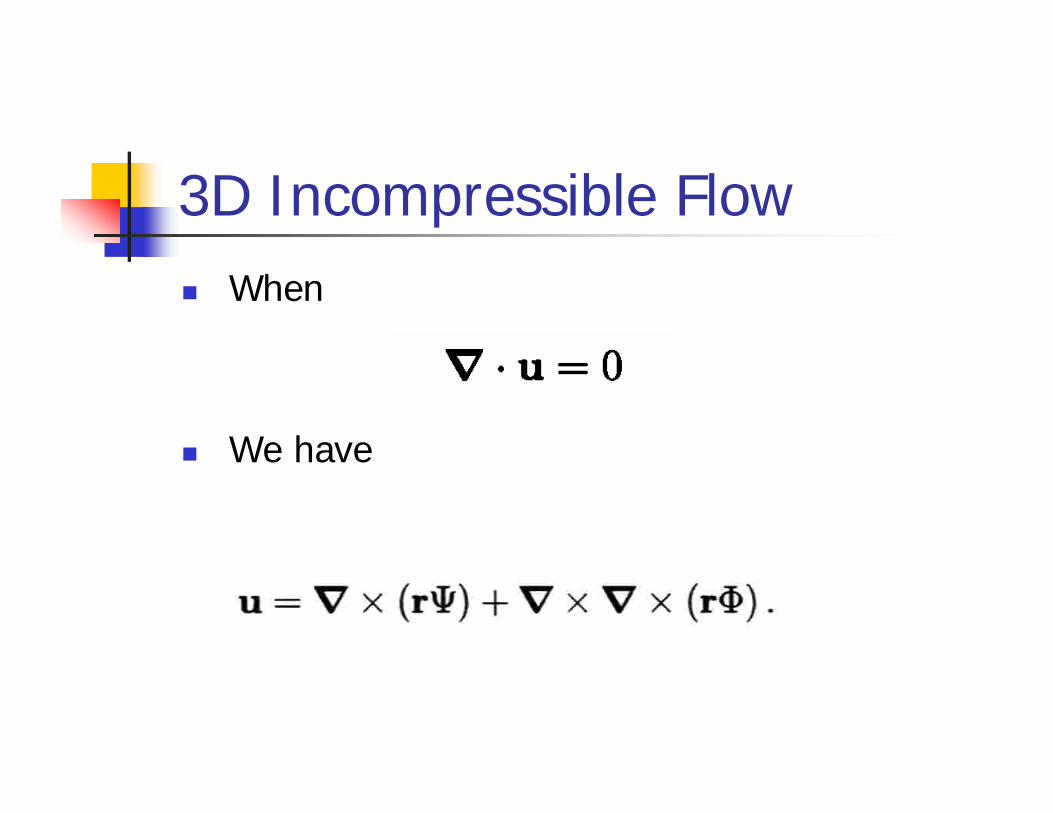
3D Incompressible Flow When

We have

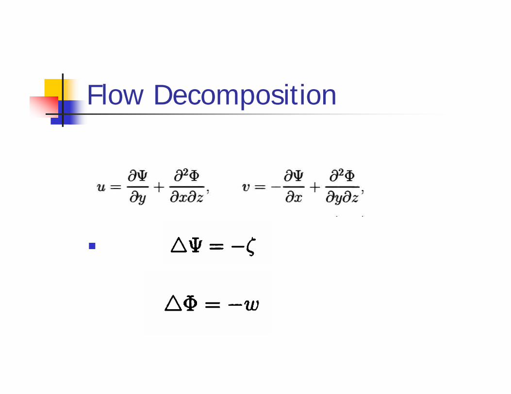
Flow Decomposition

Boundary Conditions

Basis Functions (Closed Basin)

Basis Functions (Open Boundaries)

Spectral Decomposition

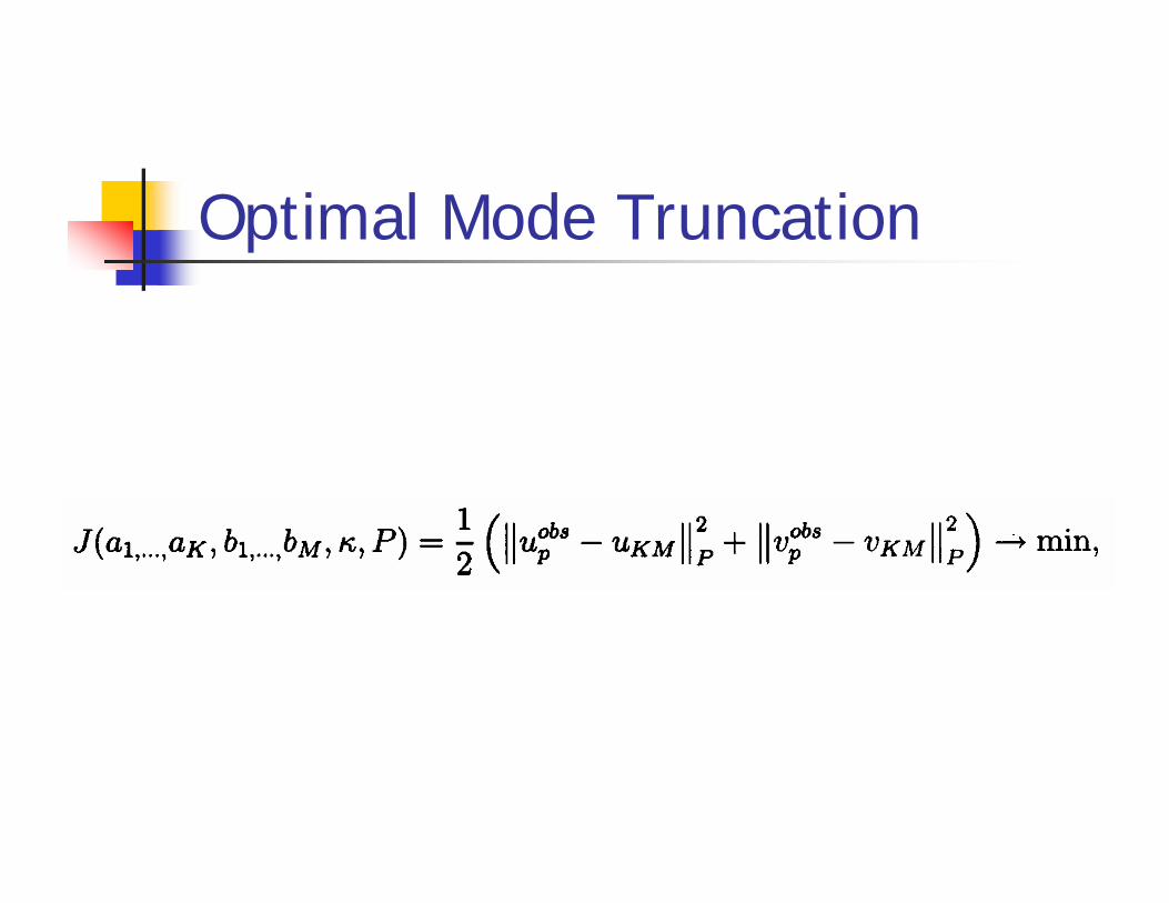
Optimal Mode Truncation

Vapnik (1983) Cost Function

Optimal Truncation

Gulf of Mexico, Monterey Bay, Louisiana-Texas Shelf

Kopt = 40, Mopt = 30

Determination of Spectral Coefficients (Ill-Posed Algebraic Equation)

Rotation Method (Chu et al., 2004)

Part-2 Application in Data Analysis Current Reversal in Louisiana-Texas Continental Shelf (LTCS)

ReferenceChu, P.C., L.M. Ivanov, and O.V. Melnichenko, 2004: Fall-winter current reversals on the Taxes-Lousianacontinental shelf, Journal of Physical Oceanography, in press.

Ocean Velocity Data 31 near-surface (10-14 m) current meter moorings during LATEX from April 1992 to November 1994

Drifting buoys deployed at the first segment of the Surface Current and Lagrangian-drift Program (SCULP-I) from October 1993 to July 1994.

Surface Wind Data

7 buoys of the National Data Buoy Center (NDBC) and industry (C-MAN) around LATEX area

Moorings and Buoys

Reconstructed and observed circulations at Station-24.

LTCS current reversal detected from SCULP-I drift trajectories.

Probability of TLCS Current Reversal for Given Period (T)

n0 ~0-current reversal n1~ 1-current reversaln2~ 2-current reversalsm ~ all realizations

Fitting the Poison Distribution

µ is the mean number of reversal for a single time interval

µ ~ 0.08

Dependence of P0, P1, P2 on T

For observational periods larger than 20 days, the probability for no currentreversal is less than 0.2.

For 15 day observational period, the probability for 1-reversal reaches 0.5

Data – Solid CurvePoison Distribution Fitting –Dashed Curve

Time Interval between Successive Current Reversals (not a Rare Event)

LTCS current reversal detected from the reconstructed velocity data

December 30, 1993

January 3, 1994

January 6, 1994

EOF Analysis of the Reconstructed Velocity Filed

0.81.10.76

2.31.41.15

4.63.31.44

6.95.63.93

9.39.510.12

74.477.180.21

10/05/94-11/29/9412/19/93-04/17/9401/21/93-05/21/93

Variance (%)EOF

Mean and First EOF Mode

Mean Circulation

1. First Period (01/21-05/21/93)

2. Second Period 12/19/93-04/17/94)

3. Third Period (10/05-11/29/94)

EOF1

1. First Period (01/21-05/21/93)

2. Second Period 12/19/93-04/17/94)

3. Third Period (10/05-11/29/94)

Calculated A1(t) Using Current Meter Mooring (solid)and SCULP-1Drifters (dashed)

8 total reversals observed

Uals ~ alongshore wind

Morlet Wavelet

A1(t)

Uals

Regression betweenA1(t) and Surface Winds

Solid Curve (reconstructed)Dashed Curve (predicted using winds)

Part-3 Application in Modeling

How Long Can a Model Predict?

ReferencesChu, P.C., L.M. Ivanov, T. M. Margolina, and O.V. Melnichenko, On probabilistic stability of an atmospheric model to various amplitude perturbations. Journal of the Atmospheric Sciences, 59, 2860-2873.Chu, P.C., L.M. Ivanov, C.W. Fan, 2002: Backward Fokker-Planck equation for determining model valid prediction period. Journal of Geophysical Research, 107, C6, 10.1029/2001JC000879.Chu, P.C., L. Ivanov, L. Kantha, O. Melnichenko, and Y. Poberezhny, 2002: Power law decay in model predictability skill. GeophysicalResearch Letters, 29 (15), 10.1029/2002GLO14891. Chu, P.C., L.M. Ivanov, L.H. Kantha, T.M. Margolina, and O.M. Melnichenko, and Y.A, Poberenzhny, 2004: Lagrangian predictabiltyof high-resolution regional ocean models. Nonlinear Processes in Geophysics, 11, 47-66.

Physical Reality

Y

Physical Law: dY/dt = h(y, t)

Initial Condition: Y(t0) = Y0

Atmospheric & Oceanic Models

X is the prediction of Y

d X/ dt = f(X, t) + q(t) X

Initial Condition: X(t0) = X0

Stochastic Forcing: <q(t)> = 0<q(t)q(t’)> = q2δ(t-t’)

Model Error

Z = X – Y

Initial: Z0 = X0 - Y0

Valid Prediction Period (VPP)

VPP is defined as the time period when the prediction error first exceeds a pre-determined criterion (i.e., the tolerance level ε).

VPP is the First-Passage Time

VPP

Conditional Probability Density Function

Initial Error: Z0

(t – t0) Random Variable

Conditional PDF of (t – t0) with given Z0

P[(t – t0) |Z0]

Two Approaches to Obtain PDF of VPP

Analytical (Backward Fokker-Planck Equation)

Practical (Optimum Spectral Analysis)

Analytical Approach

Backward Fokker-Planck Equation

Backward Fokker-Planck Equation

Model Physics Stochastic Forcing

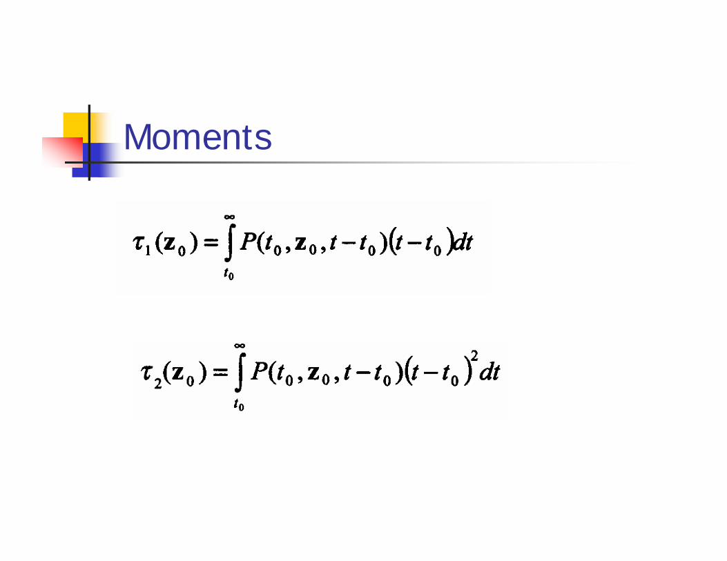
Moments

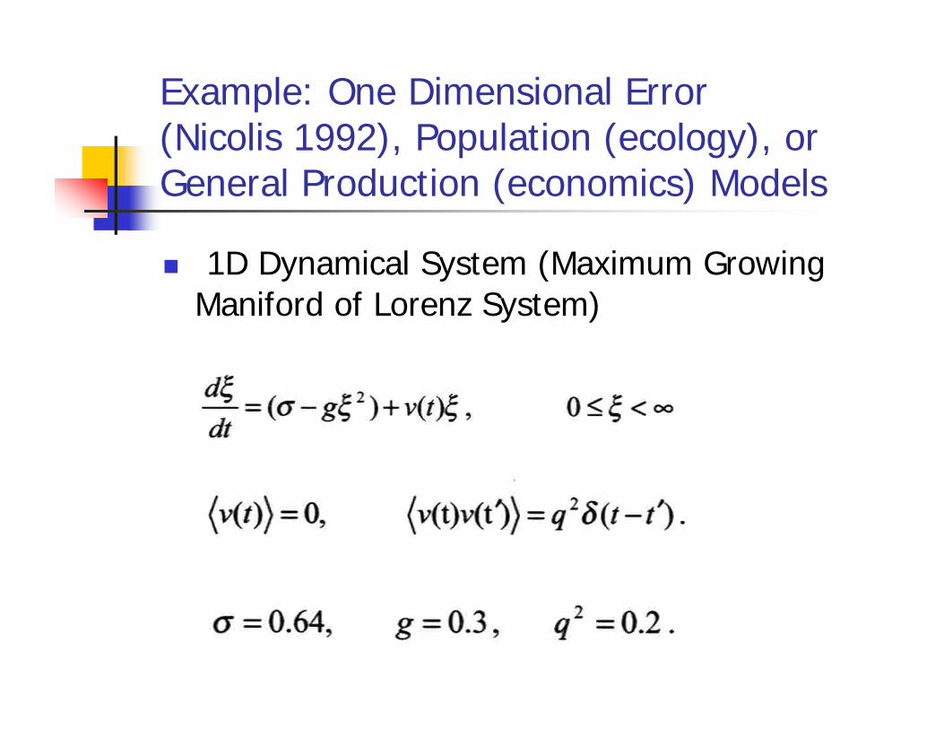
Example: One Dimensional Error (Nicolis 1992), Population (ecology), or General Production (economics) Models

1D Dynamical System (Maximum Growing Maniford of Lorenz System)

Mean and Variance of VPP

Analytical Solutions

Dependence of tau1 & tau2 on Initial Condition Error ( )

Practical Approach

Optimum Spectral Decomposition (OSD)

Gulf of Mexico Forecast System

University of Colorado Version of POM1/12o ResolutionReal-Time SSH Data (TOPEX, ESA ERS-1/2) AssimilatedReal Time SST Data (MCSST, NOAA AVHRR) AssimilatedSix Months Four-Times Daily Data From July 9, 1998 for Verification

Model Generated Velocity Vectors at 50 m on 00:00 July 9, 1998

(Observational) Drifter Data at 50 m on 00:00 July 9, 1998

Reconstructed Drift Data at 50 m on 00:00 July 9, 1998 Using the OSD Method (Chu et al. 2002 a, b, JTECH)

Error Mean and Variance

Error Mean

Error Variance

Exponential Error Growth

Classical Linear Theory

No Long-Term Predictability

Power Law

Long-Term Predictability May Occur

Statistical Characteristics of VPP

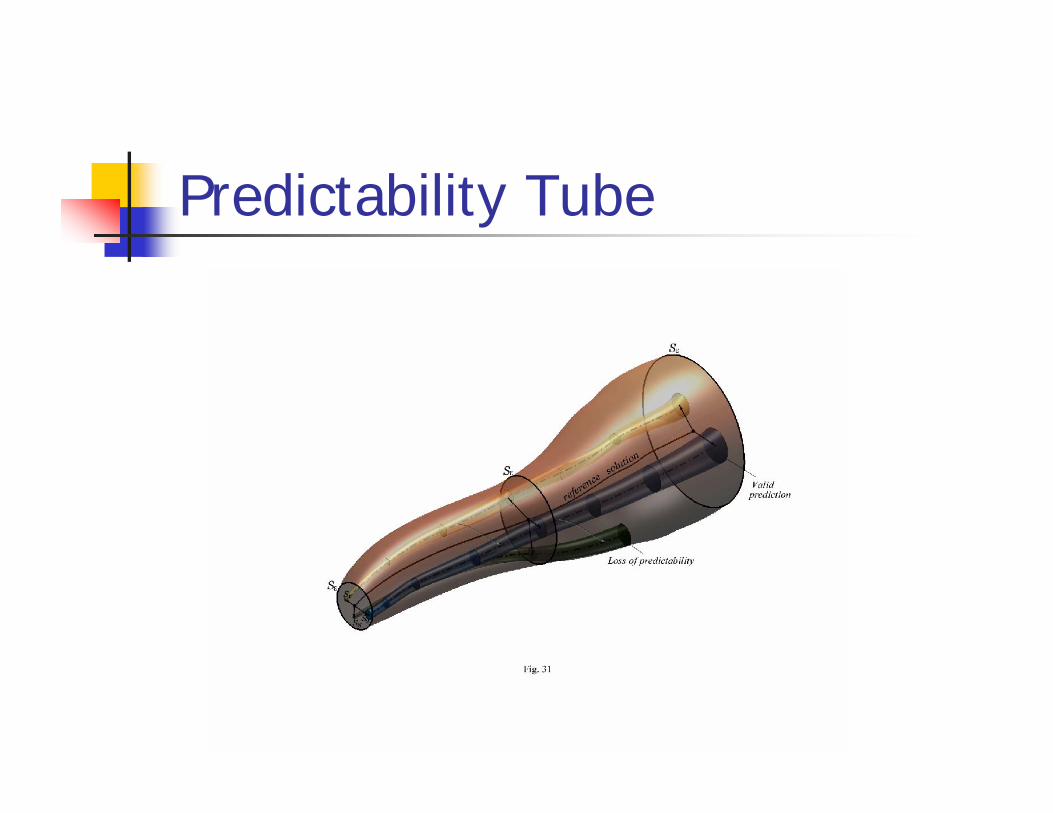
Predictability Tube

ConclusionsOSD is a useful tool for processing real-time velocity data with short duration and limited-area sampling.

The scheme can handle highly noisy data.

The scheme is model independent.

The scheme can be used for velocity data assimilation.

Phase Space Consideration