Spectral/hp element methods: Recent developments ... · 1 Spectral/hp element methods: Recent...

General rights Copyright and moral rights for the publications made accessible in the public portal are retained by the authors and/or other copyright owners and it is a condition of accessing publications that users recognise and abide by the legal requirements associated with these rights.

Users may download and print one copy of any publication from the public portal for the purpose of private study or research.

You may not further distribute the material or use it for any profit-making activity or commercial gain

You may freely distribute the URL identifying the publication in the public portal If you believe that this document breaches copyright please contact us providing details, and we will remove access to the work immediately and investigate your claim.

Downloaded from orbit.dtu.dk on: Mar 21, 2020

Spectral/hp element methods: Recent developments, applications, and perspectives

Xu, Hui; Cantwell, Chris; Monteserin, Carlos; Eskilsson, Claes; Engsig-Karup, Allan Peter; Sherwin,SpencerPublished in:Journal of Hydrodynamics

Link to article, DOI:10.1007/s42241-018-0001-1

Publication date:2018

Document VersionPublisher's PDF, also known as Version of record

Link back to DTU Orbit

Citation (APA):Xu, H., Cantwell, C., Monteserin, C., Eskilsson, C., Engsig-Karup, A. P., & Sherwin, S. (2018). Spectral/hpelement methods: Recent developments, applications, and perspectives. Journal of Hydrodynamics, 30(1), 1-22.https://doi.org/10.1007/s42241-018-0001-1

https://doi.org/10.1007/s42241-018-0001-1

https://orbit.dtu.dk/en/publications/76380ad5-6c16-4fbe-8d44-157ec6c027e7

https://doi.org/10.1007/s42241-018-0001-1

1

Spectral/hp element methods: Recent developments, applications, and perspectives * Hui Xu 1, Chris D. Cantwell 1, Carlos Monteserin 2, Claes Eskilsson 4, 5, Allan P. Engsig-Karup 2, 3, Spencer J. Sherwin 1 1. Department of Aeronautics, Imperial College London, London SW7 2AZ, UK 2. Department of Applied Mathematics and Computer Science, Technical University of Denmark, 2800 Kgs. Lyngby, Denmark 3. Center for Energy Resources Engineering (CERE), Technical University of Denmark, 2800 Kgs. Lyngby, Denmark 4. Department of Civil Engineering, Aalborg University, DK-9220 Aalborg Ø, Denmark 5. Division Safety and Transport, Research Institutes of Sweden (RISE), SE-50115 Borås, Sweden (Received December 22, 2017, Accepted December 28, 2017) © The Authors [2018] This article is published with open access at link.springer.com Abstract: The spectral/hp element method combines the geometric flexibility of the classical h-type finite element technique with the desirable numerical properties of spectral methods, employing high-degree piecewise polynomial basis functions on coarse finite element-type meshes. The spatial approximation is based upon orthogonal polynomials, such as Legendre or Chebychev polynomials,

modified to accommodate a 0 -C continuous expansion. Computationally and theoretically, by increasing the polynomial order p ,

high-precision solutions and fast convergence can be obtained and, in particular, under certain regularity assumptions an exponential reduction in approximation error between numerical and exact solutions can be achieved. This method has now been applied in many simulation studies of both fundamental and practical engineering flows. This paper briefly describes the formulation of the spectral/hp element method and provides an overview of its application to computational fluid dynamics. In particular, it focuses on the use of the spectral/hp element method in transitional flows and ocean engineering. Finally, some of the major challenges to be overcome in order to use the spectral/hp element method in more complex science and engineering applications are discussed. Key words: High-precision spectral/hp elements, continuous Galerkin method, discontinuous Galerkin method, implicit large eddy simulation Project Leader

Spencer Sherwin is Professor of Computational Fluid Mechanics and the Head of Aerodynamics Section in the Department of Aeronautics at Imperial College London. He received his MSE and Ph. D. from the Department of Mechanical and Aerospace Engineering Department at Princeton University in 1995. Prior to this he received his BEng from the Department of Aeronautics at Imperial College London in 1990. In 1995, he joined the Department of Aeronautics at Imperial College as a lecturer and subsequently became a full professor in 2005. Over the past 27 years he has specialised in the development and application of advanced parallel spectral/hp

* Biography: Hui Xu (1981-), Male, Ph. D. Corresponding author: Hui Xu, E-mail: [email protected]

element methods for flow around complex geometries with a particular emphasis on vortical and bluff body flows, biomedical modelling of the cardiovascular system and more recently in industrial practice through the partnerships with McLaren Racing and Rolls Royce. Professor Sherwin’s research group also develops and distributes the open-source spectral/hp element package Nektar++ (www.nektar.info) which has been applied to direct numerical simulation, large eddy simulation and stability analysis to a range of applications including vortex flows of relevance to offshore engineering and vehicle aerodynamics as well as biomedical flows associated with arterial atherosclerosis. He has published numerous peer- reviewed papers in international journals covering topics from numerical analysis to applied and fundamental fluid mechanics and co-authored a highly cited book on the spectral/hp element method. Since 2014 Prof. Sherwin has served as an associate editor of the

Available online at https://link.springer.com http://www.jhydrod.com/

2018,30(1):1-22 https://doi.org/10.1007/s42241-018-0001-1

2

Journal of Fluid Mechanics. He is a Fellow of the Royal Aeronautical Society, a Fellow of the American Physical Society and in 2017 he was elected a Fellow of the Royal Academy of Engineering.

Introduction Over the past few decades, computational fluid

dynamics (CFD) has become increasingly powerful and has therefore been seen as the natural starting point to investigate a variety of mathematical and physical problems in science and engineering. Traditio- nally, “low-order methods” with up to second-order spatial accuracy have been widely adopted as the default implementation for the simulation of fluid flows, often based around the Reynolds averaged Navier-Stokes (RANS) equations. This approach has achieved a great deal of success in many applications due to its well-established robustness and efficiency. However, as the demands on the accuracy of CFD outputs have increased, such as requiring the solution of the unsteady flow equations in complex geometries, low-order methods are less able to provide the necessary level of precision in capturing transient dynamics, as compared to higher accuracy schemes for a given computational cost. Therefore, there is currently a great interest in the development and application of high-order methods such as the spectral/hp element discretisation.

Finite element methods are widely used across a broad range of engineering and scientific disciplines. They can be categorised into three classes[1, 2]: (1) the classical h-version finite element method, (2) the spectral element method, or p-version finite element method, (3) the hp-version finite element method, called the spectral/hp element method. Once the computational domain is partitioned into a non-overlapping element set, the spectral/hp element method employs a “spectral-like” approach in each element, representing the solution through a basis of polynomials. Therefore, the spectral/hp element method combines the advantages of the spectral element method, in terms of the properties of accuracy and rapid convergence, with those of the classical h-version finite element method, that allows complex geometries to be effectively captured. Compared with traditional low-order finite element schemes, the spectral/hp element method can provide an arbitrary order of spatial-approximation accuracy under the assumption of sufficient smoothness of the solution. It therefore combines the advantages of the low-order finite element method family, whilst also providing an additional attractive higher-precision, approximation for solving partial differential equations[3, 4]. Recent studies also indicate that the compact nature of the spectral/hp element method is well-placed to take advantage of modern multi-core and many-core

computing hardware[5, 6]. All of the above properties have positioned the spectral/hp element method as an attractive numerical strategy for obtaining high- precision solutions with a relatively low computational cost.

The spectral/hp element method is gaining increasing traction in the field of CFD[3], and it has achieved great success in both direct and large eddy simulation (LES) of complex flows[7-11]. It has also been successfully applied to a broad range of other applications in various research fields, for instance, cardiac electro-physiology[12], solid mechanics[13, 14], porous media[15] and oceanographic modelling[16].

One of the challenges of these methods is that they are more challenging to implement than low- order methods. There are now, however, now a number of open-source packages which encapsulate the complexities of the method. One such package that the authors have been developing is Nektar++, a cross-platform spectral/hp element framework (http:// www.nektar.info) which has made high-order finite element methods more accessible to the broader com- munity and can be used to solve a range of the emerging challenges in high-fidelity scientific computations[4]. It enables the construction of high-order discretisations for solving a wide range of partial differential equations, supporting hybrid meshes, for example triangles and quadrilaterals or tetrahedra, prisms, pyramids and hexahedra. The current software package includes a number of pre-written scalable solvers, including for incompressible flow, compressible flow, shallow water equations, acoustic perturbation equations and others.

In this paper, we present a review of the state-of- the-art of the spectral/hp element method, and its applications. In Section 1, we briefly describe the spectral/hp element method and discuss the numerical advantages and robustness of the method in solving partial differential equations. In Section 2, we high light some of the implementation challenges of the method in order to achieve computational efficiency and discuss potential solutions through our efforts with Nektar++. In Section 3, we then provide a survey of the applications in transitional flows and waves (wave propagation and wave-body interaction) in ocean engineering to which the spectral/hp element method has been applied. Finally, in Section 4, we conclude with further discussions and some perspectives on future directions.

1. Spectral/hp element method In this section, we provide an overview of the

mathematical foundations of the spectral/hp element method. A more detailed derivation of the mathematical theory can be found in Ref. [3] but is beyond the scope of this paper.

3

1.1 Overview of method Spectral/hp element discretisations are the under-

pinning approximation for both continuous and discontinuous Galerkin formulations and can be constructed in 1-D, 2-D and 3-D. To obtain a general view of the method we can consider the example in Fig. 1. At the bottom of this figure we observe a triangulation of the British Isles. In general, the computational mesh can comprise of a mix of different shaped elements which could be triangles and quadrilaterals in two dimensions, and tetrahedra, pyramids, prisms and hexahedra in three dimensions. Within each element we develop a polynomial expansion, as represented in the lower-right of Fig. 1, where we observe all of the expansion modes to represent a fourth-order polynomial using a modal or hierarchical expansion basis. For Continuous Galerkin (CG) expansions, the design of these elements typically has the property of being decomposed into boundary and interior modes so that 0 -C continuity can be achieved by matching boundary expansion modes that have support on the edges of the element. The interior modes are necessarily defined to be zero on the boundaries. There are a number of ways of developing the polynomial expansion within an element iK . In the

Fig. 1 Illustration of the construction of a 2-D fourth-order

0 -C continuous modal triangular expansion basis using a generalised tensor-product procedure

example shown in Fig. 1 we illustrate the popular construction using a tensor product of 1-D expansions which are defined in the regular regions K and K which can then be mapped to the physical elemental regions using the mapping ( ) . Tensor-based

expansions are very popular in quadrilateral and hexahedral regions but require some modification for triangular or tetrahedral regions using a Duffy[17] or collapsed-coordinate system[3]. It is possible to define polynomial expansions that are hierarchical/modal in construction, much like a small-scale spectral expansion, or alternatively one can use a nodal basis where the expansion is defined at a specific set of points (often related to Gaussian quadrature) and only one expansion mode has a unit value, whilst all other expansions bases are zero, at this point. This provides a Kronecker delta property to the expansion which can be useful when evaluating non-linear products. Again, for triangular elements the construction of a nodal basis is more involved and typically requires the use of a generalised Vandemonde matrix to relate them to a known expansion which is often of a modal construction[18].

Once a polynomial expansion has been defined in each element, the approach used to “bolt together” these individual expansions defines the approximation

method. For example, if one enforces a 0 -C continuous expansion by ensuring the polynomial expansion is continuous across elemental boundaries we obtain the classical CG method. Alternatively, if one does

not directly enforce the expansions to be 0 -Ccontinuous but ensures appropriate flux quantities are continuous between elements, one can construct a so-called Discontinuous Galerkin (DG) scheme[3, 18, 19]. 1.2 Outline of mathematical formulation In general, we consider the numerical solution of partial differential equations (PDEs) of the form

= 0Lu on a domain , which may be geometrically complex, for some solution u . Practically, takes the form of a d - dimensional finite element mesh consisting of elements Ki, embedded in a space

of dimension d̂ , such that ˆ 3d d , with = i iK

and i jK K

is an empty set or an interface between

elements of dimension d d . We solve the PDE problem in the weak sense and, in general, |

iKu must

be smooth with at least a first-order derivative, we therefore require that |

iKu is in the Sobolev space 1, 2 1( ) ( )i iW K H K [20]. For a continuous discretisation,

we additionally impose continuity along element interfaces. For illustrative purposes, we assume that it can be expressed as follows:

4

find 1( )u H such that ( , ) = ( )a u v l v ,

1( )v H

(1)

where ( , )a is a bilinear form, ( )l

is a linear form

and 1( )H is formally defined as

1 2 2( ) : { ( ) | ( ), 1}H v L D u L

(2)

To solve this problem numerically, we consider solutions in a finite-dimensional subspace V

1( )H and cast our problem as

find 1( )u H such that ( , ) = ( ),a u v l v

v V

(3) augmented with appropriate boundary conditions. For a projection which enforces continuity across elements, we impose the additional constraint that

0V C . We assume the solution can be represented

as ˆ( ) = ( )n nnu x u x , a weighted sum of N trial

functions ( )n x defined on and our problem

becomes that of finding the coefficients ˆnu . The ap-

proximation u does not directly give rise to unique

choices for the coefficients ˆnu . To achieve this, we

place a restriction on the residual =R Lu that its

2L inner product, with respect to the test functions ( )n x , is zero. For a Galerkin projection we choose

the test functions to be the same as the trial functions, that is =n n . As outlined previously, to construct

the global basis n we first consider the contribu-

tions from each element in the domain. Each iK is

mapped from a standard reference space = [ 1,1]dK by a parametric mapping :e iK K given by

e= ( ) x , where K is one of the supported region

shapes, and are d - dimensional coordinates rep-

resenting positions in a reference element, distinguis-

hing them from x which are d̂ - dimensional coordinates in the Cartesian coordinate space. The mapping need not necessarily exhibit a constant Jacobian, supporting deformed and curved elements through an isoparametric mapping. For triangular, tetrahedral, prismatic and pyramid elements, the Duffy transform[17] is used and operations, such as calculating derivatives, map the coordinate system to the non- collapsed coordinate system.

A local polynomial basis is constructed on each reference element with which to represent solutions. A one-dimensional order-P basis is a set of polynomials

( )p , 0 p P , defined on the reference segment.

The particular choice of basis is usually made based on its mathematical or numerical properties and may be modal or nodal in nature. For 2-D and 3-D regions, a tensorial basis may be used, where the polynomial space is constructed as the tensor-product of 1-D bases on segments, quadrilaterals or hexahedral regions. In particular, a common choice is to use a modified hierarchical Legendre basis, given as a function of one variable by

1( ) =

2p

, = 0p

(4a)

1,1

1

1 1+( ) = ( )

2 2p pP

, 0 p P

(4b)

1+

( ) =2p

, =p P

(4c)

which supports the aforementioned boundary-interior decomposition and therefore improves numerical efficiency when solving the globally assemble dsystem. Equivalently, p

could be defined by the Lagrange

polynomials through the Gauss-Lobatto-Legendre quadrature points which would lead to a traditional spectral element method. On a physical element iK the discrete approximation u

to the solution u may be expressed as

1ˆ( ) = ([ ] ( ))n n enu x u x

(5)

where ˆnu are the coefficients from Eq. (1), obtained

through projecting u onto the discrete space. There- fore, we restrict our solution space to

1: { ( ) ( )}i

p iKV u H u K P

(6)

where ( )p iKP

is the space of order - p polynomials

on iK . Elemental contributions to the solution may

be assembled to form a global solution through an assembly operator. In a CG setting, the assembly operator sums contributions from neighbouring

elements to enforce the 0 -C continuity requirement.

In a DG formulation, such mappings transfer flux values from the element interfaces into global solution vector.

5

Fig. 2 Propagation of a cone initial condition using a DG formulation of the advection equation. After one rotation, we see the solution using a = 2P , = 6P and = 8P order approximations

1.3 What are the beneficial properties of using a

spectral/hp element method? For smooth problems one of the benefits of a

spectral/hp formulation is often quoted as the exponential rate of convergence one observes when increasing the polynomial order of the approximation, providing the solution has sufficient regularity. In practice, the good approximation properties are also realised in terms of the better diffusion and dispersion properties one observes as you increase the polynomial order. This is exemplified in Fig. 2 where we have taken an initial condition of a Gaussian and advected it under a rotational velocity field for one revolution. We then observe the solution of a DG approximation of the linear advection problem using a

= 1P , = 3P and = 8P order approximation with 128, 32 and 8 elements, respectively. We see from this simple test that the shape is far less diffused in the

= 8P problem when compared to the = 2P discretisation, even though the overall number of degrees of freedom is comparable.

Recently, a comparison between high-order flux reconstruction and the industrial-standard solver STAR-CCM+, was made, in which the accuracy and computational cost of flux reconstruction (FR) methods in PyFR and STAR-CCM+, for a range of test cases including scale-resolving simulations of turbulent flow were investigated[21]. The results from both PyFR and STAR-CCM+ show that third-order schemes can be more accurate than second-order schemes for a given cost. Moreover, advancing to higher-order schemes on GPUs with PyFR was found to offer even further accuracy vs cost benefits relative to industry- standard tools. These demonstrate the potential utility of high-order methods on GPUs for scale-resolving simulations of unsteady turbulent flows.

1.4 Using the spectral/hp element method in marginally resolved problems In the previous sections, we outlined the underl-

ying formulation of the spectral/hp element methodology and we now describe some of the state-of-the- art developments necessary for simulating problems which are only marginally resolved. These tend to arise at higher Reynolds numbers, which generally promote greater levels of turbulence that cannot realistically be captured, even on the latest parallel computers. This leads to the build-up of energy in the larger resolved scales, due to the inability of the discretisation to fully capture the smaller scales of the flow. This is addressed with two techniques. The first involves performing the numerical integration of nonlinear terms consistently. Even with this, non-linear interactions may still lead to an artificial build-up of energy in the smaller resolved scales. A second technique is then to apply a spectral filtering, known as spectral vanishing viscosity, to dampen such energies. 1.4.1 Dealiasing

Dealiasing strategies have been observed to be effective in enhancing the numerical stability when solving problems using the spectral/hp element method[22-26]. The errors are typically caused by insufficient quadrature employed in the Galerkin discretisation of nonlinear terms[3]. When the simulation is not sufficiently well- resolved, this leads to energy in the shorter length scales to be transferred back into the longer length scales. When simulations are well- resolved, the numerical errors created by insufficient quadrature are negligible[23, 24]. However, in marginally resolved or under-resolved simulations, aliasing errors may significantly pollute the solution[23]. As discussed in Ref. [26], there are three kinds of aliasing sources: (1) PDE aliasing, which relates to quasi-linear and non-linear terms[23]. (2) Geometrical aliasing, which arises due to deformed/curved elements.

(3) Interface-flux aliasing, in the case of discontinuous methods[26].

We start by giving an example from incompressible viscous flow past a NACA 0012 wing tip at a

Reynolds number of 6=1.2 10Re , originally discussed in Ref. [26], to demonstrate the aliasing error in the near surface region. Figure 3 illustrates the dynamics of the flow by showing the iso-contours of helicity with a = 3P approximation. In the boundary region, prismatic elements are employed while tetrahedral elements are used in the rest of the domain. Figure 4, shows the first two kinds of aliasing errors. In Fig. 4(a), 30% aliasing error with respect to the

6

magnitude of the nonlinear terms is observed and in Fig. 4(b) we show a close up of regions with high geometrical aliasing error near the wing surface where 600% error is observed. The aliasing errors in this numerical calculation significantly pollute the solution and cause it to very rapidly become numerically unstable. Fig. 3 Helicity for an incompressible viscous flow over a

NACA 0012 wing[26] Fig. 4 PDE aliasing errors at 30% of the magnitude of the

nonlinear terms (a) and close up regions near the wing surface showing geometric aliasing errors (b)[26]

We can categorise dealiasing techniques into two strategies: (1) Local dealiasing: PDE-dealiasing through consistent integration of the nonlinear terms only[23, 26]. (2) Global dealiasing: PDE- and geometrical- dealiasing through consistent integration of all the terms of the discretisation[26].

The phrase consistent integration refers to polynomial nonlinearities, where it is effectively possible to know a priori the number of quadrature points necessary for the integration to be exact[23, 27]. There- fore, the non-linearities can be consistently integrated. For non-polynomial functions, as typically arise in the Euler equations, the concept of consistent integration is not well defined since it is impossible to fully control the quadrature error. We refer to the reader to Ref. [26] for a more complete discussion of these strategies as well as a discussion of interface aliasing. 1.4.2 Spectral vanishing viscosity

As previously discussed, it is well known that spectral/hp element discretisations generally lead to approximations that have low dissipation and low dispersion[3] per degree of freedom when compared to lower-order methods. In solving advection-diffusion

equations and nonlinear partial differential equations such as advection-dominated flows, at marginal reso- lutions, oscillations appear that may render the computation unstable[3]. Artificial viscosity has been used in may discretisation methods to suppress wiggles associated with high wavenumbers, for example hyperviscosity has been broadly and effectively used in simulations using the Fourier method. A related concept is the so-called spectral vanishing viscosity (SVV), which was originally proposed based on a second-order diffusion (convolution) operator for spectral Fourier methods[28]. The SVV concept was originally motivated through the inviscid Burgers equation where an additional diffusion term was added, i.e.

2 ( , ) ( , )( , ) + =

2

u x t u x tu x t D

t x x x

(7)

where ( 0) is a viscosity amplitude and D is a

viscosity kernel, which may be nonlinear, can be a function of x and is only activated for high wave numbers. With a small amount of controlled dissipation, spectral accuracy can be retained. This approach was extended to the Navier-Stokes equations by Karamanos and Karniadakis[29] and Kirby and Sherwin[30] and has also been investigated and applied to large eddy simulation by Pasquetti[31, 32]. To provide some intuition about the influence of SVV, we show in Fig. 5 an example from Ref. [30] of applying SVV to the parabolic equation

2= + ( )VV

uu S u

t

(8)

on = [0,2] [0,2] with 5= 10 and periodic boun-

dary conditions. The initial condition is given by

( , , = 0) = sin( )sin( )u x y t x y , in which a perturba-

tion is introduced. A total of sixteen quadrilateral elements (four per direction) with 15th order polynomials per element direction were used. The following “classical” 1-D SVV kernel is employed,

= 0D , cutp P

(9a)

2

2cut

( )= exp

( )

p PD

p P

, cutp P

(9b)

where P is the total number of modes employed and

cutP is the cutoff polynomial order. SVV with the

kernel function D can be regarded as a low-pass filter. We see that the SVV dissipation added to the high mode numbers with respect to the spectral

7

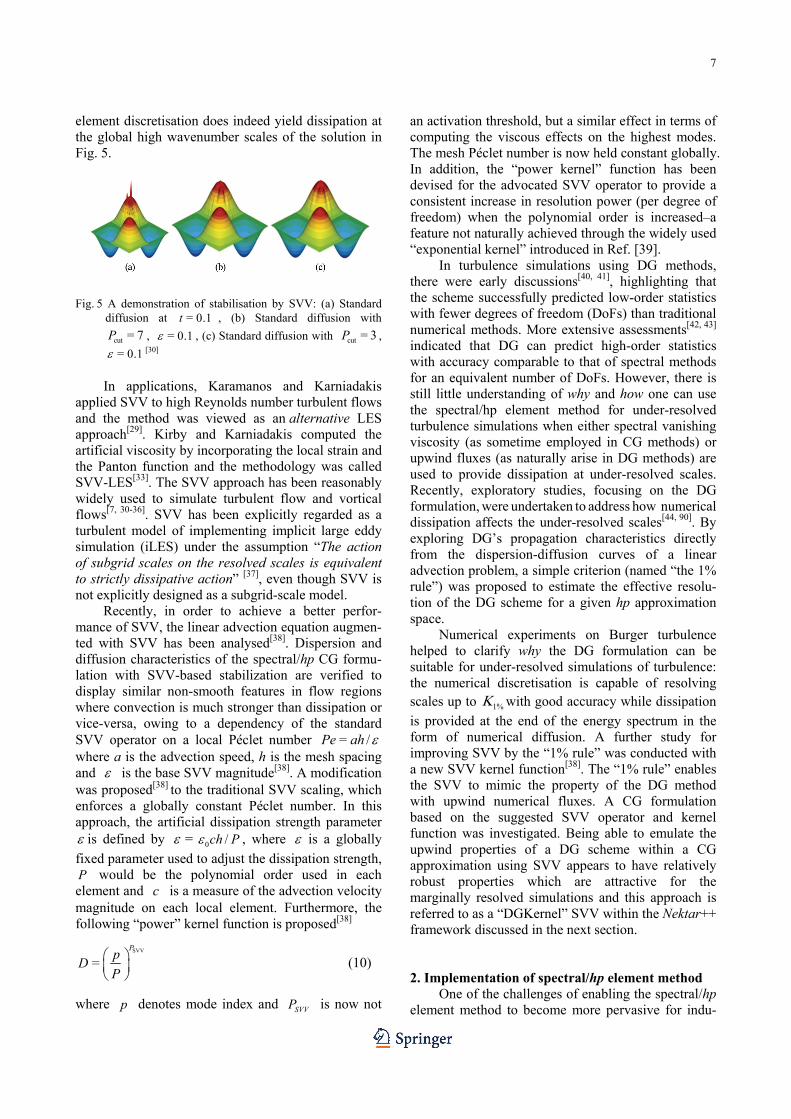
element discretisation does indeed yield dissipation at the global high wavenumber scales of the solution in Fig. 5.

Fig. 5 A demonstration of stabilisation by SVV: (a) Standard diffusion at = 0.1t , (b) Standard diffusion with

cut = 7P , = 0.1 , (c) Standard diffusion with cut = 3P ,

= 0.1 [30] In applications, Karamanos and Karniadakis applied SVV to high Reynolds number turbulent flows and the method was viewed as an alternative LES approach[29]. Kirby and Karniadakis computed the artificial viscosity by incorporating the local strain and the Panton function and the methodology was called SVV-LES[33]. The SVV approach has been reasonably widely used to simulate turbulent flow and vortical flows[7, 30-36]. SVV has been explicitly regarded as a turbulent model of implementing implicit large eddy simulation (iLES) under the assumption “The action of subgrid scales on the resolved scales is equivalent to strictly dissipative action” [37], even though SVV is not explicitly designed as a subgrid-scale model.

Recently, in order to achieve a better performance of SVV, the linear advection equation augmented with SVV has been analysed[38]. Dispersion and diffusion characteristics of the spectral/hp CG formulation with SVV-based stabilization are verified to display similar non-smooth features in flow regions where convection is much stronger than dissipation or vice-versa, owing to a dependency of the standard SVV operator on a local Péclet number = /Pe ah where a is the advection speed, h is the mesh spacing and is the base SVV magnitude[38]. A modification was proposed[38] to the traditional SVV scaling, which enforces a globally constant Péclet number. In this approach, the artificial dissipation strength parameter is defined by = 0 /ch P , where is a globally

fixed parameter used to adjust the dissipation strength, P would be the polynomial order used in each element and c is a measure of the advection velocity magnitude on each local element. Furthermore, the following “power” kernel function is proposed[38]

SVV

=P

pD

P

(10)

where p denotes mode index and SVVP is now not

an activation threshold, but a similar effect in terms of computing the viscous effects on the highest modes. The mesh Péclet number is now held constant globally. In addition, the “power kernel” function has been devised for the advocated SVV operator to provide a consistent increase in resolution power (per degree of freedom) when the polynomial order is increased–a feature not naturally achieved through the widely used “exponential kernel” introduced in Ref. [39].

In turbulence simulations using DG methods, there were early discussions[40, 41], highlighting that the scheme successfully predicted low-order statistics with fewer degrees of freedom (DoFs) than traditional numerical methods. More extensive assessments[42, 43] indicated that DG can predict high-order statistics with accuracy comparable to that of spectral methods for an equivalent number of DoFs. However, there is still little understanding of why and how one can use the spectral/hp element method for under-resolved turbulence simulations when either spectral vanishing viscosity (as sometime employed in CG methods) or upwind fluxes (as naturally arise in DG methods) are used to provide dissipation at under-resolved scales. Recently, exploratory studies, focusing on the DG formulation, were undertaken to address how numerical dissipation affects the under-resolved scales[44, 90]. By exploring DG’s propagation characteristics directly from the dispersion-diffusion curves of a linear advection problem, a simple criterion (named “the 1% rule”) was proposed to estimate the effective resolution of the DG scheme for a given hp approximation space.

Numerical experiments on Burger turbulence helped to clarify why the DG formulation can be suitable for under-resolved simulations of turbulence: the numerical discretisation is capable of resolving scales up to 1% with good accuracy while dissipation

is provided at the end of the energy spectrum in the form of numerical diffusion. A further study for improving SVV by the “1% rule” was conducted with a new SVV kernel function[38]. The “1% rule” enables the SVV to mimic the property of the DG method with upwind numerical fluxes. A CG formulation based on the suggested SVV operator and kernel function was investigated. Being able to emulate the upwind properties of a DG scheme within a CG approximation using SVV appears to have relatively robust properties which are attractive for the marginally resolved simulations and this approach is referred to as a “DGKernel” SVV within the Nektar++ framework discussed in the next section. 2. Implementation of spectral/hp element method

One of the challenges of enabling the spectral/hp element method to become more pervasive for indu-

8

strial and environmental problems is the implementa- tional complexity of the methods. One of the overarc- hing aims of the Nektar++ project is to provide an efficient framework upon which a broad range of physical processes can be modelled using these approaches. With this in mind, we outline some of efficiency challenges associated with implementing these methods for practical use and detail some suitable solutions in the context of Nektar++. 2.1 Nektar++ overview

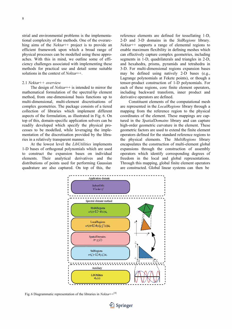
The design of Nektar++ is intended to mirror the mathematical formulation of the spectral/hp element method, from one-dimensional basis functions up to multi-dimensional, multi-element discretisations of complex geometries. The package consists of a tiered collection of libraries which implement different aspects of the formulation, as illustrated in Fig. 6. On top of this, domain-specific application solvers can be readily developed which specify the physical processes to be modelled, while leveraging the implementation of the discretisation provided by the libraries in a relatively transparent manner.

At the lowest level the LibUtilities implements 1-D bases of orthogonal polynomials which are used to construct the expansion bases on individual elements. Their analytical derivatives and the distributions of points used for performing Gaussian quadrature are also captured. On top of this, the

reference elements are defined for tessellating 1-D, 2-D and 3-D domains in the StdRegions library. Nektar++ supports a range of elemental regions to enable maximum flexibility in defining meshes which can effectively capture complex geometries, including segments in 1-D, quadrilaterals and triangles in 2-D, and hexahedra, prisms, pyramids and tetrahedra in 3-D. For multi-dimensional regions expansion bases may be defined using natively 2-D bases (e.g., Lagrange polynomials at Fekete points), or though a tensor-product construction of 1-D polynomials. For each of these regions, core finite element operators, including backward transform, inner product and derivative operators are defined.

Constituent elements of the computational mesh are represented in the LocalRegions library through a mapping from the reference region to the physical coordinates of the element. These mappings are captured in the SpatialDomains library and can capture high-order geometric curvature in the element. These geometric factors are used to extend the finite element operators defined for the standard reference regions to the physical elements. The MultiRegions library encapsulates the construction of multi-element global expansions through the construction of assembly operators which identify corresponding degrees of freedom in the local and global representations. Through this mapping, global finite element operators are constructed. Global linear systems can then be

Fig. 6 Diagrammatic representation of the libraries in Nektar++[4]

9

solved using a number of direct and iterative linear algebra techniques. Iterative approaches, such as the preconditioned conjugate gradient method, solve a system through the repeated action of the operator, providing scope for a range of performance optimisa- tions, discussed in Section 2.3.

While the central concept captured in Nektar++ are high-order spectral/hp element spatial discretisations, high-order time integration algorithms are also implemented to allow for highly accurate transient simulations. These include fully explicit, implicit and mixed implicit-explicit (IMEX) schemes. 2.2 Combined spectral/hp-Fourier discretisation

While the spectral/hp element method exhibits some of the numerical characteristics of a pure spectral method, the use of the latter is still preferred in the case of regular geometries such as rectangles and cuboidal domains. This situation occurs widely in many, particularly fundamental, hydrodynamics problems. In Nektar++, we leverage this by allowing for a mixed spectral/hp-Fourier discretisation. In this confi- guration, geometrically homogeneous coordinate directions are represented with a truncated Fourier expansion, while coordinate directions with geometric complexity use the spectral/hp element discretisation. This has the effect of decoupling the individual Fourier modes, allowing the spectral/hp operator to be applied independently within each component of each Fourier mode. The Fourier decomposition also enables parallel decomposition of the modes to different processes[45]. Combined with the parallelisation of the spectral/hp element discretisation this leads to a hybrid paralle- lism. An open challenge here is identifying the optimal parallelisation of such mixed-discretisation domains to achieve optimal performance.

The GlobalMappings library further extends this discretisation strategy by supporting geometries in which a coordinate direction can be transformed to a homogeneous representation by an analytical function. This enables more complex geometries to be discre- tised using this efficient formulation. 2.3 From h to p efficiently

One of the challenges in implementing the spectral/hp method is achieving computational performance across a broad range of polynomial orders. The classic approach to implementing linear finite element operators is to assemble the global form of the operator and act directly on the global degrees of freedom. This is performant since each mesh vertex has a high valency and the assembly operation dramatically reduces the size of the global linear system used within the iterative solver. With increasing polynomial order, this reduction is less and the

memory indirection associated with the global operator leads to reduced through-put and degraded performance.

A number of studies[46-49] have concluded that for higher polynomial orders, one should instead scatter the global degrees of freedom back onto their local elemental representation and perform the action of the operator in an element-wise fashion using a matrix- vector operation. This enables a more compact representation of the operator in memory, greater cache- locality in applying the operator and a reduction in overall memory usage. At very high polynomial orders, the size of the local operator grows as

40( )P .

A more efficient approach in these cases is to take advantage of the tensor-product construction of the operators to decompose the elemental operator into a sequence of 1-D operators, known as sum-factorisation. Algebraically, this corresponds to a sequence of matrix-matrix operations which, besides the reduction in floating operation count, can be generally more efficiently implemented.

Recalling the construction of the local elemental operators as the reference region operator, transformed under a geometric mapping, one can exploit the decomposition of the elemental operators into these constituent parts. The Collections library in Nektar++ exploits this decomposition on groups of similar elements (same shape and expansion basis) by applying first the geometric factors associated with the operator, before acting with the reference region operator on all of the elements in the group simul- taneously[50]. This effectively replaces a sequence of matrix-vector operations with a single matrix-matrix operation, reducing data movement and improving floating-point performance. This decomposition can be applied both to the local elemental matrix representation as well as the sum-factorisation approach. 2.4 High-order mesh generation

For complex 3-D geometries, the generation of high-order curved meshes along solid surfaces is a challenging topic[51-55]. Approaches for generating unstructured high-order meshes, extending coarse linear grids to incorporate high-order curvature, are a

Fig. 7 Splitting a reference prismatic element and applying the mapping to obtain a high-order layer of prisms from the macro-element[51]

10

Fig. 8 Surface mesh of a NACA 0012 wing geometry at polynomial order = 5P . The coarse prismatic boundary layer is highlighted in blue (a) and the refined boundary layer which uses three layers and a progression ratio = 3r (b)[51]

Fig. 9(a) Turbulent channel flow

Fig. 9(b) Turbulent pipe flow relatively new development[52, 56, 57]. The main challenge is robustness, since near-wall curvature must be introduced in such a way as to prevent the generation of self-intersecting elements[51]. Recently, several methods have been proposed to cope with high-order curvilinear boundary layer meshing, namely (1) the isoparametric approach[51], (2) the variational approach[53], and (3) the thermo-elastic analogy[54]. In the isoparametric approach, a reference element is mapped to a physical element with the supplied curvature information. The generation of a boundary layer mesh is achieved by splitting the reference element along the wall normal coordinate and then applying the mapping from a reference element to a physical element yielding the desired boundary layer mesh as illustrated in Fig. 7. In Fig. 8, a mesh for the NACA0012 aerofoil profile is shown which is generated by the isoparametric approach[51]. In the variational approach, a functional which defines a measure of energy over mesh and takes the mesh displacement and its derivatives as its arguments, is

minimised using a nonlinear optimisation strategy[53]. It is demonstrated that the variational framework is efficient for both mesh quality optimisation and untangling of invalid meshes. In order to circumvent the drawback of elastic-model based methods which are used to tackle element self-intersection, a thermo- elastic analogy, as an extension of the elastic formulation, is proposed to “heat” or “cool” elements. The thermo-elastic formulation leads to an additional degree of robustness, which shows the potential to significantly improve meshing[54]. NekMesh, which is a mesh generation and manipulation utility bundled with Nektar++, supports these strategies for high- order mesh generation. 3. Applications

In this section, we illustrate some typical applications of spectral/hp element methods in fluid mechanics, typically in hydrodynamics. Some examples will be given through use of the pre-written solvers in Nektar++. 3.1 The incompressible Navier-Stokes equations We first introduce the incompressible Navier- Stokes equations on a bounded domain which allows one to solve the governing equations for viscous Newtonian fluids governed by

2+ = +pt

u

u u u

(11a)

= 0 u

(11b) with appropriate boundary conditions. In Nektar++, a velocity correction scheme is employed, which uses a splitting/projection method where the velocity and the pressure are decoupled[58]. In the original approach, a stiffly stable time integration scheme was proposed. Briefly, high-order splitting schemes comprise of three steps involving explicit evaluation of the non-linear terms, followed by the implicit solution of the pressure Poisson system and finally solving a series of Helmholtz problems to enforce the viscous terms and velocity boundary conditions. Time integration is handled using a generic time-stepping framework, utilising one of a number of implicit-explicit (IMEX) time-integration schemes, the details of which can be found in Ref. [59]. 3.2 Transitional flows

In the past few decades, the spectral/hp element method has been applied to laminar and transitional flows[58, 60-64]. As discussed earlier, the advantages of the spectral/hp element method are its low numerical dissipation and dispersion errors, which allow indivi-

11

dual flow structures to be accurately captured over long time periods. Combined with the development of effective stabilisation techniques (e.g., SVV or filter- based stabilisation[65]), the spectral/hp element method has in most recent years proved effective in modelling turbulent flow[33, 66-70].

Transitional problems are those in which turbulence dominates the flow domain, or in which the transition to turbulence is a fundamental aspect of the simulation. Here we provide a survey of the range of studies undertaken using the spectral/hp element method in relation to transitional flows, focusing on (1) turbulence, (2) separated flows, (3) hydrodynamic stability, and (4) vortical flows and high Reynolds number wingtip vortices. 3.2.1 Turbulent flows

As noted in Ref. [4], highly resolved turbulent simulations were traditionally undertaken using spectral methods, imposing strong geometrical restrictions. Spectral/hp element methods alleviate this constraint although, as discussed in Section 2, when the domain of interest has a geometrically homogeneous direction, a combination of the spectral/hp element method and the traditional spectral method is still particularly advantageous[45, 71]. A benchmark simulation of turbulent flow over a periodic hill has been performed using Nektar++. It is challenging to resolve accurately due to the detach- ment of the fluid from the smooth surface and the generation of a recirculation region downstream of the hill[4]. A 2-D mesh of 3 626 quadrilateral elements with = 6P in the streamwise direction was constructed, and a Fourier pseudo-spectral method with 160 collocation points in the spanwise direction was employed to perform the simulation at a Reynolds number 2 800. Excellent agreement with the benchmark statistics was obtained. With the quasi-3D solver, turbulent channel and pipe flows have also been accurately simulated and validated[45], these are illustrated in Fig. 9 and are used as benchmark cases in Nektar++.

Recently, a global mapping technique has been developed which allows the simulation of fluid flows with geometrically periodic variation along homogeneous directions[8, 11]. A typical example is to simulate turbulent flows induced by a localised surface deformation in the boundary layer[11]. The computational domain is illustrated in Fig. 10(a) and the turbulent flow which forms downstream of the surface deformation is shown in Fig. 10(b). The freestream unit Reynolds number is 1.2106

and the reference free-stream velocity is 18m/s. The laminar-turbulent transition is initialised by the nonlinear process of upstream Tollmien-Schlichting (TS) disturbance breakdown to turbulence downstream of the surface

indentation. The disturbance is generated by a disturbance strip as illustrated in Fig. 10(a), which has a vibration frequency of 172 Hz and is used to mimic the TS disturbance by the receptivity mechanism. The numerical calculations of this case are validated with an experimental study for which excellent agreement is obtained.

Fig. 10 An illustration of the computational domain for the turbulent simulation in a boundary layer (a) and laminar-turbulent transition triggered by TS instability in a boundary layer. The iso-surfaces indicate the different pressure levels[11]

3.2.2 Separated flows

Flow separation can be one of the most important topics in fluid mechanics, due to its relevance to aerodynamic performance in many engineering applications. There are typically two kinds of separations: geometrical, where the flow separates from a sharp obstacle in the flow, and pressure-induced, depending on the pressure gradient over a smooth surface. For both kinds of separation, the spectral/hp element method has been used to accurately capture detach- ment and reattachment points, e.g., laminar flow in a channel expansion[72], turbulent separation in a 3-D diffuser[25], the flow around a wall-mounted square cylinder[73], flows over periodic hills[74], small separation bubbles induced by localised imperfections[11, 75]. Practically, the studies of separated flows are always accompanied by turbulent flows due to the occurrence of sensitive instabilities induced by the geometrical discontinuity.

Recently, with the global mapping technique, direct numerical simulations of the flow around wings with spanwise waviness were investigated to explore its effect on the wing performance[9, 76]. The geometries are based on a NACA0012 profile with a small modification to obtain zero-thickness trailing edge to overcome meshing challenges. The wavy geometries were obtained by applying the following coordinate transformation to the straight infinite wing

12

2

= cos2

hx x z

(12)

Fig. 11 The geometry of a wavy wing with / = 0.1h c and

/ = 0.5d [9]

Fig. 12 Flow properties around the wing with an attack angle o12 , / = 0.1h c and / = 0.5d [9]

where h is the waviness peak-to-peak amplitude, is its wavelength, x is the physical coordinate in the cord direction, and x and z are the chordwise and spanwise coordinates in the computational domain in Fig. 11. At a very low Reynolds number 1 000, for moderate angles of attack, the waviness leads to decreases in both drag and lift forces, which lead to a decrease in the lift-to-drag ratio and a suppression of the fluctuating lift coefficient[9]. The physical mechanism behind these were explained. In Fig. 12(a), the recirculation regions are shown and the visualisation was made considering the regions where streamwise velocity is negative. In Fig. 12(b), the coloured contours represent spanwise velocity at the plane =x

0.33 , which is close to the location of the leading edge in the peak of the waviness at = 0.05x , depicting how the flow moves away from the waviness peak in the lower portion of the wing and it moves towards it in the upper part. A further study was undertaken at Reynolds numbers 10 000 and 50 000 for different attack angles through highly resolved direct numerical simulations[76], which provides a better understanding of wing performance with the use of spanwise waviness. 3.2.3 Hydrodynamic stability

In addition to solving the fully non-linear incompressible Navier-Stokes equations in Nektar++, the solution of the linearised incompressible Navier- Stokes equations is also supported to enable global flow stability analyses to be performed with respect to a steady or a time-periodic base flow. This process identifies whether such flows are susceptible to a fundamental change of state when an infinitesimal disturbance is introduction. The linearised incompressible Navier-Stokes equations take the following form

2+ + = + +p ft

u

U u u U u ,

= 0 u

(13) where u is the perturbation and U denotes the base flow or a time-dependent periodic flow which are sampled at regular intervals and interpolated. For stability analysis, suitable boundary conditions should be imposed. The linear evolution of a perturbation under Eq. (13) can be expressed as

= A( ) ( )t tt

u

u

(14)

with an initial condition (0)u . If the base flow U

is steady, the perturbation ( )tu be expressed by

eigenmode solutions of ( )A t as follows

( ) = exp( ) +c.c.j jt tu u

(15)

The dominant eigenvalues and eigenmodes of the operator ( )A t are defined by solutions to the follo-

wing equation

( ) =j j jA t u u

(16)

The leading eigenvalue j is used to detect the

global stability of the flow. Using a similar approach, the operator ( )A t

for the adjoint form of the lineari-

13

sed Navier-Stokes evolution operator can be used to examine the receptivity of the flow and, in combination with the direct mode, identify the sensitivity to base flow modification and local feedback. The direct and adjoint methods can be combined to explore convective instabilities over different time horizons in a flow by computing the leading

eigenmodes of ( )( )A A known as transient growth

analysis. The eigenvalues and eigenmodes of ( )A and ( )( )A A

can be solved directly if the dimen-

sions of the matrices are small. Practically, time- stepper-based methodologies, based on Arnoldi itera- tion methods[77], can be more efficient for complex problems[78-81] than direct calculation of the eigenvalue spectrum from the linearised Navier-Stokes operator. To illustrate the direct stability analysis with a classic example, we calculated the dominant mode of the two-dimensional flow past a circular cylinder at Fig. 13 Direct stability analysis of 2-D flow past a circular

cylinder at = 50Re

= 50Re . We show the two components of the base flow in Figs. 13 (a) and 13(b) and the two components of the dominant direct mode in Figs. 13 (c) and 13 (d). The leading eigenmode is characterised by the asymmetry in the streamwise component and symmetry in the cross-stream component. We also observe the

spatial distribution of the modes, with the leading direct modes extending far downstream of the cylinder. Recently, instability methods using the spectral/hp element method have been employed for investigating the stability of vortical flows and controlling wakes of flows past bluff bodies[82-84]. With the linearised Navier-Stokes equations, the interaction between instability waves and surface distortion in a 2-D and 3-D boundary layer have been precisely investigated[10, 11, 75].

Fig. 14 Tip vortex of an elliptic hydrofoil 3.2.4 Vortical flows and wingtip vortex

Simulating and understanding vortical flows are vital in hydrodynamics and aerodynamics. In many applications, manipulation of vortices in the vicinity of flow boundaries is crucial for improving performance in engineering practice[7, 85-89]. Developing a better understanding of the near wake of the vortex, lying within one chord length of the trailing edge, is essential in understanding the complex flow structure interactions[7], which is also crucial in understanding cavitation in vortical structures generated by hydro propellers[86]. Computationally, in high Reynolds number flows, accurate numerical simulations of these kinds of vortical structures are challenging for the traditional numerical methods due to numerical dissipation. A recent study in which wingtip vortices were simulated demonstrated that the adjustable and controllable low-dissipation properties of the spectral/ hp element method were beneficial for modelling and simulating vortical flows[7, 44, 90].

To illustrate the ability of the spectral/hp element method to accurately capture vortical flows at a Reynolds number 1.2106, a rectangular wing with a NACA0012 profile, is investigated with a rounded wing cap (consequently, a longer semispan where the wing is thickest) and a blunt trailing edge[7]. The results showed better correlation with experimental results than previous numerical results, both in terms of the static pressure distribution, prediction of the jetting velocity, vortex spanwise location, and the ability to resolve the secondary vortex interaction with the main wingtip vortex. The iLES method based on SVV has been shown to be a compelling alternative for computing complex vortex-dominated flows, such as the wingtip vortex, motivating its use for complex

14

industrially relevant cases where high-fidelity computational fluid dynamics can become an enabling tech- nology.

Fig. 15 Vorticity components x , y and z directions at

the section / = 1.06x c

Built on the confidence of simulating the NACA0012 wingtip vortex, recently, an initial simulation with a Reynolds number 1.217106

is currently being conducted to simulate the tip vortex of an elliptic hydrofoil where the incident flow attack angle is o7 . The tip vortex structure is illustrated by the iso-surfaces of the total pressure in Fig. 14. The contour figures of the vorticity components are shown at the section / = 1.06x c in Fig. 15 and the origin is located at the tip of the hydrofoil. In Fig. 15(a), the vortex core is shown in axial vorticity x and

tangential and spanwise vorticity components ( y

and z ) are shown in dipoles in Figs. 15(b) and 15(c).

This calculation will be used to provide vortex core pressure for studying cavitation in a vortex structure. The numerical results will be going to be compared with experimental data. 3.3 Waves in ocean engineering This section is devoted to outlining recent progress in spectral/hp element modelling of wave propagation and wave-body interaction. For water waves propagation, the fully nonlinear potential flow (FNPF) equations is the fundamental governing equation and can be derived from the Navier-Stokes equations by assuming inviscid and irrotational flow. One of the main challenges in the last decade have focused on use of spectral/hp element methods for coastal engineering[91], and the development of robust and efficient solvers with support for unstructured meshes to capture realistic shore lines, geometric features, and adapt meshes to relevant features of the solution[92]. 3.3.1 Fully nonlinear potential flow

Finite elements are widely used for solving the FNPF equations[93-96], but the use of spectral/hp elements remains scarse. The first attempt to solve the FNPF equations using spectral/hp elements is due to Robertson and Sherwin[97] using an arbitrary Lagrangian Eulerian (ALE) approach for the free water surface in a 2-D setting. Solving the FNPF equations is non-trivial, due to the need to evolve a set of highly nonlinear free surface boundary conditions in a robust way, together with the efficiency solution of a Laplace problems-possibly-in large ocean areas. For spectral/hp element models, Robertson and Sherwin identified a mesh asymmetry problem associated with triangulation of the fluid domain, which gives rise to real-valued eigenvalues and thus represented a severe instability problem. This was handled by adding a diffusive term in the kinematic free surface boundary condition proportional to the mesh asymmetry, but at the cost of reduced convergence rates. The problem of mesh asymmetry which dest- roys the dispersion relation was circumvented by Engsig-Karup et al.[98, 99] by solving the FNPF equations in a - transformed domain[94] using a single layer of quadrilaterals in 2-D and prisms in 3-D. The FNPF model was shown to exhibit exponential convergence even for steep nonlinear stream function waves which most simpler wave models cannot handle. To stabilise the nonlinear simulations, it was found that the quartic nonlinear terms in the free surface equation need to be integrated exactly and for the steep waves a mild (1%) modal filter could be used to remove high frequency noise that can stem from aliasing in nonlinear terms for marginal resolution, and the gradient recovery steps that reconstruct

15

the gradients of the solution (e.g., velocities) from the 0C approximations.

Letting denote the horizontal gradient operator, the velocity potential satisfy the Laplace equa-

tion

2

2+ = 0

z

(17)

with time-dependent free surface boundary conditions on =z

given in the Zakahrov[100]

+ (1+ ) = 0w wt

(18)

21+ + [ + (1+ )] = 0

2g

t

(19)

and zero normal flow on the bottom =z h and on

structures b

= 0n

(20)

Here is the free surface elevation, w the vertical

velocity, h the still water depth and g the accelera- tion of gravity. The σ-transformed FNPF solver as presented in Ref. [99] has been implemented in the Nektar++ framework in order to allow for larger-scale modelling[101]. The solution is advanced explicitly in time by solving the free-surface equations. The computed +1n are used as Dirichlet condition for the

Laplace equation at =z . After solving for the

velocity potential, +1nw is obtained by a 0C gra-

dient recovery as +1nw is needed to advance the free surface conditions another time step. Explicit time- stepping schemes are effective for FNPF as the time- step restriction is not dependent on the horisontal mesh size, but only on the vertical resolution and water depth[98]. A σ-transformed FNPF solver is well- suited for large-scale wave propagation simulations, since re-meshing is avoided. Also, an intrinsic property of FNPF solvers is the ability to get accurate kinematics in all of the fluid domain as a part of the solutions, which is relevant for wave-induced load predictions on marine structures. The - transformed FNPF solver can be used for computing e.g., short- wave disturbances in ports, see Fig. 16, and wave scattering from bottom mounted vertical cylinders, see Fig. 17.

The use of - transformed domains excludes any truncated bodies in the domain. In order to handle

Fig. 16 Snap shot of free surface elevation in the Port of Visby

using fifth order method Fig. 17 Wave scattering of regular waves by a cylinder. Wave

propagating from (a) to (b) arbitrarily shaped bodies in the domain the mixed- Eulerian-Lagrangian (MEL) approach should be used and there are ongoing efforts to implement a SEM based on the MEL approach. In Ref. [102] a work- around on the mesh asymmetry problem associated with the MEL was presented. By using hybrid meshes consisting of a single layer of vertically aligned quads (in 2-D) at the free surface, the eigenvalues were shown to be purely imaginary for any triangulation of the inner field. When using higher-order local polynomial expansions as done in the spectral/hp element method, a local re-meshing (movement of quadrature points inside the local elements) as well as global re-meshing (movement of vertices) are needed in the MEL approach. An example of a spectral/hp element simulation using MEL for wave-body interaction are illustrated in Fig. 18. Here a solitary wave is passing over a horizontal submerged cylinder.

16

Fig. 18 Solitary wave passing a submerged horizontal

cylinder[102] 3.3.2 Shallow water wave equations

While the application of spectral/hp element method for FNPF equations is emerging, in the field of depth-integrated shallow water long wave equations there is a wider use of spectral/hp elements methods. These equations can be derived from the FNPF equations by expanding the velocity potential in terms of the vertical coordinate and integrating the Laplace problem over the fluid depth. This removes the vertical dependence of the problem. Non-hydrostatic wave equations (such as Boussinesq-, Serre- or Green-Naghdi-type equations) are used for wave propagation and transformation in nearshore regions. The dispersive effects are included in the equations through higher-order mixed and spatial derivatives.

Eskilsson and Sherwin presented the first spectral/hp model for 1-D Boussinesq-type equations[103], and later in 2-D[104]. In the latter study was illustrated that the use of high-order schemes is computationally efficient compared to low-order methods for long- time integration. This is general knowledge, mathema- tically proven in Ref. [105], but the importance is accenturated in wave equation where the numerical dispersion error must be kept small compared to the physical dispersion terms. Additional spectral/hp studies of weakly dispersive Boussinesq equations are Refs. [106, 107]. Engsig-Karup et al.[108-110] solved a set highly dispersive and nonlinear Boussinesq-type equations. More recently the interest has turned toward Green-Naghdi type equations due to their description of nonlinearity and a number of spectral/hp element methods have been put for- ward[111-113]. We note that all the above models are based on high-order DG methods.

The classical Boussinesq equations due to Pere- grine[114] read

+ [( + ) ] = 0h ut

(21)

2

+ + +6

u h ug u u

t t

2 ( )

= 02

h hu

t

(22)

where u is the horizontal velocity. There exists a pre-written solver for the Peregrine equations in Nektar++. The equations are solved in terms of conservative variables and the solution scheme is using the wave-continuity step as introduced in Ref. [104]. First the advection part is approximated and used in an intermediate step. In the intermediate step the dispersive terms are reformulated into a Helmholtz equation in terms of the auxiliary variable =q

(d )t u , in which = +d h . Subsequently, a pro-

jection back to conservative variables is performed. The Boussinesq equations can be used for computing the generation of higher harmonics. A classical example is the semi-circular shoal case, see Fig. 19.

With regard to non-dispersive, hydrostatic wave equations the shallow water equations (SWE) are typically used in marine applications to predict tidal forcing but can also be used for other long wave phenomena such as tsunami and storm-surge predictions. For tsunami modelling hp-adaptive DG models have been presented in order to resolve the shock wave propagation in detail[116-118]. However, the main bulk of work on spectral/hp element methods for the

17

SWE are linked to numerical weather prediction or ocean circulation where the SWE is used as a stepping stone towards solving the 3-D primitive equations[119-125]. Fig. 19 Higher harmonics generation on a semi-circular

shoal[115]

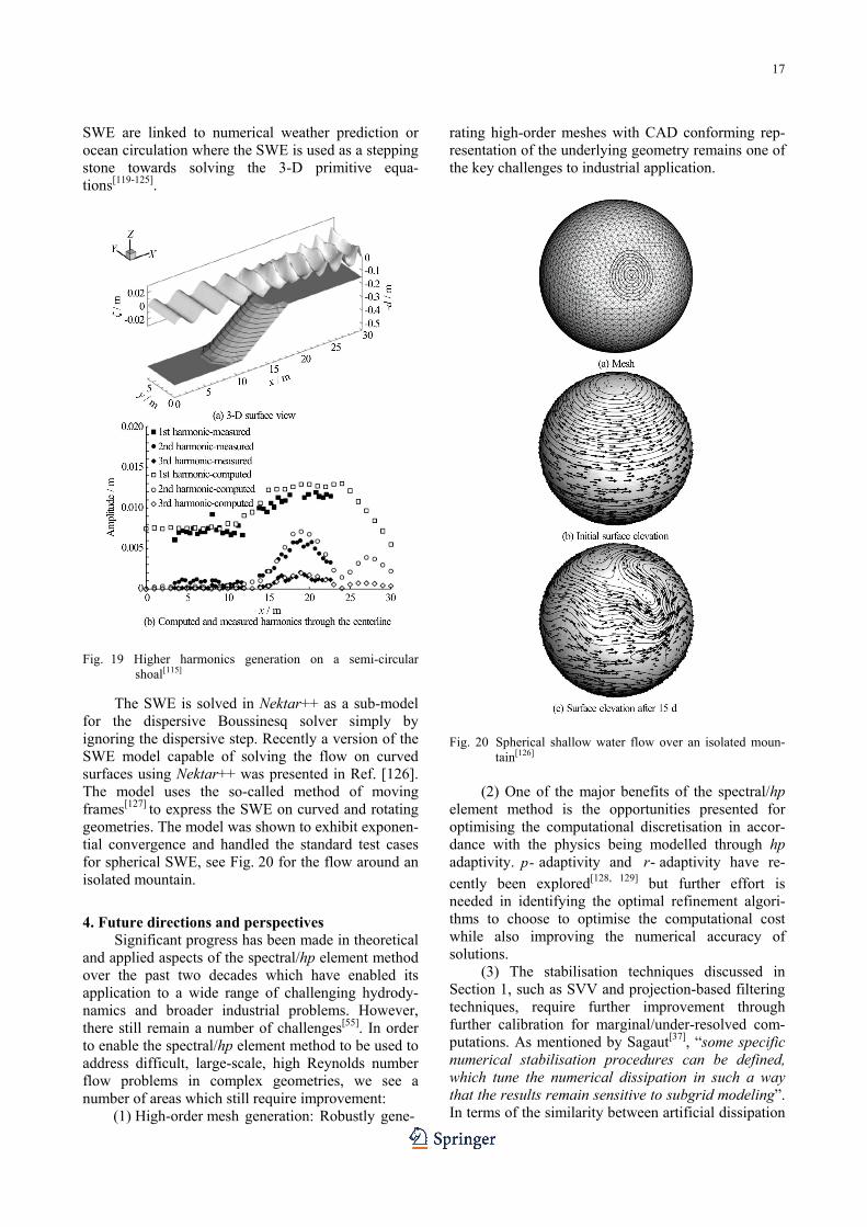
The SWE is solved in Nektar++ as a sub-model for the dispersive Boussinesq solver simply by ignoring the dispersive step. Recently a version of the SWE model capable of solving the flow on curved surfaces using Nektar++ was presented in Ref. [126]. The model uses the so-called method of moving frames[127] to express the SWE on curved and rotating geometries. The model was shown to exhibit exponential convergence and handled the standard test cases for spherical SWE, see Fig. 20 for the flow around an isolated mountain.

4. Future directions and perspectives Significant progress has been made in theoretical

and applied aspects of the spectral/hp element method over the past two decades which have enabled its application to a wide range of challenging hydrodynamics and broader industrial problems. However, there still remain a number of challenges[55]. In order to enable the spectral/hp element method to be used to address difficult, large-scale, high Reynolds number flow problems in complex geometries, we see a number of areas which still require improvement: (1) High-order mesh generation: Robustly gene-

rating high-order meshes with CAD conforming representation of the underlying geometry remains one of the key challenges to industrial application. Fig. 20 Spherical shallow water flow over an isolated moun-

tain[126]

(2) One of the major benefits of the spectral/hp element method is the opportunities presented for optimising the computational discretisation in accor- dance with the physics being modelled through hp adaptivity. -p adaptivity and -r adaptivity have re-

cently been explored[128, 129] but further effort is needed in identifying the optimal refinement algorithms to choose to optimise the computational cost while also improving the numerical accuracy of solutions.

(3) The stabilisation techniques discussed in Section 1, such as SVV and projection-based filtering techniques, require further improvement through further calibration for marginal/under-resolved computations. As mentioned by Sagaut[37], “some specific numerical stabilisation procedures can be defined, which tune the numerical dissipation in such a way that the results remain sensitive to subgrid modeling”. In terms of the similarity between artificial dissipation

18

and the direct energy cascade model, some numerical stabilisation techniques can be used to perform “no-model” large eddy simulations (iLES). However, Sagaut stated that “certain studies have shown that, for coarse grids, i.e., high values of the numerical cutoff length, increasing the order of accuracy of the upwind scheme can lead to a degradation of the results[130]”. The proposed “DGKernel”, which emu- lates the upwind properties of a DG scheme, still requires more detailed calibration for a range of high-Reynolds fluid flows.

(4) Verification and Validation of spectral/hp element simulations for under-resolved computations: The use of stabilisation techniques, such as SVV, allows us to interpret the under-resolved numerical calculations as implicit large eddy simulation. How- ever, we need to continue to investigate how the stabilisation methods and numerical properties interact to ensure the benefits of high-precision are not destroyed through artificial/ numerical pollution.

In the context of hydrodynamics applications, there is substantial opportunity for gaining an impro- ved understanding of a wide range of physical mecha- nisms through the use of the spectral/hp element method. In particular: (1) Tip vortex modelling: As indicated in Ref. [7], without the accurate modelling of the 3-D boundary layer, the developing vortex remained challenging to compute accurately, even for the advanced RANS models correcting for the high degree of curvature in the flow. In addition, accurately capturing the low- pressure region within the vortex core and sustaining this low pressure even just one chord length downstream of the trailing edge is particularly challenging. As demonstrated[7], the SVV-based iLES method has been shown to be potential alternative for computing complex unsteady vortex dominated flows. Simulating vortical flows using the spectral/hp element method with the concept of the SVV-based iLES can be regarded as an interesting alternative method in hydrodynamics.

(2) Implicit large eddy simulation: A notable effort has been made to refine the SVV-based strategy for implementing under-resolved simulations of high Reynolds fluid flows[38, 44]. This strategy has a great potential to provide high fidelity iLES computations for a broad range of applications in hydrodynamics. (3) Fluid-structure interaction: As indicated in Refs. [131-135], spectral elements offer superior wave propagation capabilities, which has been used for simulations of fluid-structure interaction[133, 134, 136]. Interaction subject to surface waves can be attractive.

(4) Cavitating flow: Recently, discontinuous spectral/hp element method has been implemented for the efficient and accurate simulation of multiphase flows[137]. The compressible Navier-Stokes equations,

coupled with a highly realistic equation of state, are solved by a DG spectral element method for flows with cavitation. In Nektar++, the DG method and the flux reconstruction approach have been used to solve the compressible Navier-Stokes equations. This therefore provides a basis to apply the spectral/hp element method in applications of cavitating flows.

(5) Free surface flows: As is well known free surface flows can be modelled as a depth average “shallow-water” approach or using ALE moving mesh techniques. Spectral/hp element method has been used to treat these two kinds of free surface flows[97, 138-141]. For the second free surface problem, discontinuous spectral/hp element methods hava great potential in applications[139-141, 143, 144], especially when h/p-adaptivity is employed. Acknowledgments

The authors kindly thank the Executive Editor- in-Chief Prof. Lian-di Zhou for the invitation to contribute this review article and Dr. Wei Zhang for his contribution to conducting the tip-vortex simulation. H.X. and S.J.S would like to acknowledge support under EPSRC (Grant No. EP/L000407/1).

This article is distributed under the terms of the Creative Commons Attribution 4.0 International License (http://creativecommons.org/licenses/by/4.0/), which permits unrestricted use, distribution, and reproduction in any medium, provided you give appropriate credit to the original author(s) and the source, provide a link to the Creative Commons license, and indicate if changes were made.

References [1] Babuška I., Suri M. The p- and h-p versions of the finite

element method, an overview [J]. Computer Methods in Applied Mechanics and Engineering, 1990, 80(1): 5-26.

[2] Babuška I., Suri M. The p and h-p versions of the finite element method, basic principles and properties [J]. Computer Methods in Applied Mechanics and Enginee- ring, 1994, 36(4): 578-632.

[3] Karniadakis G., Sherwin S. Spectral/hp element methods for computational fluid dynamics [M]. Second Edition, New York, USA, Oxford University Press, 2005.

[4] Cantwell C. D., Moxey D., Comerford A. et al. Nektar++: An open-source spectral/hp element framework [J]. Computer Physics Communications, 2015, 192: 205-219.

[5] Yakovlev S., Moxey D., Kirby R. M. et al. To CG or to HDG: A comparative study in 3D [J]. Journal of Scientific Computing, 2016, 67(1): 192-220.

[6] King J., Yakovlev S., Fu Z. S. et al. Exploiting batch processing on streaming architectures to solve 2D elliptic finite element problems: A hybridized discontinuous Galerkin (HDG) case study [J]. Journal of Scientific Computing, 2014, 60(2): 457-482.

[7] Lombard J. E. W., Moxey D., Sherwin S. J. et al. Implicit

19

large-eddy simulation of a wingtip vortex [J]. AIAA Journal, 2016, 54(2): 506-518.

[8] Serson D., Meneghini J. R., Sherwin S. J. Velocity-correction schemes for the incompressible navier-stokes equations in general coordinate systems [J]. Journal of Computational Physics, 2016, 316: 243-254.

[9] Serson D., Meneghini J. R., Sherwin S. J. Direct numerical simulations of the flow around wings with spanwise waviness at a very low Reynolds number [J]. Computers and Fluids, 2017, 146: 117-124.

[10] Xu H., Lombard J.-E. W., Sherwin S. J. Influence of localised smooth steps on the instability of a boundary layer [J]. Journal of Fluid Mechanics, 2017, 817: 138-170.

[11] Xu H., Mughal S. M., Gowree E. R. et al. Destabilisation and modification of Tollmien-Schlichting disturbances by a three-dimensional surface indentation [J]. Journal of Fluid Mechanics, 2017, 819: 592-620.

[12] Cantwell C. D., Yakovlev S., Kirby R. M. et al. High- order spectral/hp element discretisation for reaction- diffusion problems on surfaces: Application to cardiac electrophysiology [J]. Journal of Computational Physics, 2017, 257: 813-829.

[13] Szabó B., Babuka I. Finite element analysis [M]. New York, USA: John Wiley and Sons, Inc., 1991.

[14] Moxey D., Ekelschot D., Keskin Ü. et al. A thermo-elastic analogy for high-order curvilinear meshing with control of mesh validity and quality [C]. Procedia Engineering, 23rd International Meshing Roundtable (IMR23), London, UK, 2014, 82: 127-135.

[15] Comerford A., Chooi K. Y., Nowak M. et al. A combined numerical and experimental framework for determining permeability properties of the arterial media [J]. Biome- chanics and Modeling in Mechanobiology, 2015, 14(2): 297-313.

[16] Eskilsson C., Sherwin S. J. Spectral/hp discontinuous Galerkin methods for modelling 2D Boussinesq equations [J]. Journal of Computational Physics, 2016, 212(2): 566-589.

[17] Duffy M. G. Quadrature over a pyramid or cube of integrands with a singularity at a vertex [J]. SIAM Journal on Numerical Analysis, 1982, 19(6): 1260-1262.

[18] Hesthaven J. S., Warburton T. Nodal discontinuous Galerkin methods [M]. New York, USA: Springer-Verlag, 2008.

[19] Reed W. H., Hill T. R. Triangular mesh methods for the neutron transport equation [R]. Technical report, Los Alamos National Laboratory, 1973, lA-UR-73-479.

[20] Adams R. A. Sobolev spaces [M]. New York, USA: Aca- demic Press, 1975.

[21] Vermeire B., Witherden F., Vincent P. On the utility of GPU accelerated high-order methods for unsteady flow simulations: A comparison with industry-standard tools [J]. Journal of Computational Physics, 2017, 334: 497-521.

[22] Gottlieb D., Orszag S. A. Numerical analysis of spectral methods: Theory and applications [M]. Philadelphia, USA: Society for Industrial and Applied Mathematics, 1977.

[23] Kirby R. M., Karniadakis G. E. De-aliasing on non-uni- form grids: Algorithms and applications [J]. Journal of Computational Physics, 2003, 191(1): 249-264.

[24] Kirby R. M., Sherwin S. J. Aliasing errors due to quadratic nonlinearities on triangular spectral/hp element discretisations [J]. Journal of Engineering Mathematics, 2006, 56(3): 273-288.

[25] Malm J., Schlatter P., Henningson D. S. Coherent structures and dominant frequencies in a turbulent three- dimensional diffuser [J]. Journal of Fluid Mechanics, 2012, 699: 320-351.

[26] Mengaldo G., Grazia D. D., Moxey D. et al. Dealiasing techniques for high-order spectral element methods on regular and irregular grids [J]. Journal of Computational Physics, 2015, 299: 56-81.

[27] Cockburn B., Hou S. C., Shu C. W. The Runge-Kutta local projection discontinuous Galerkin finite element method for conservation laws. IV. The multidimensional case [J]. Mathematics of Computation, 1990, 54(190): 545-581.

[28] Tadmor E. Convergence of spectral methods for nonlinear conservation laws [J]. SIAM Journal on Numerical Analysis, 1989, 26(1): 30-44.

[29] Karamanos G. S., Karniadakis G. E. A spectral vanishing viscosity method for large-eddy simulations [J]. Journal of Computational Physics, 2000, 163(1): 22-50.

[30] Kirby R. M., Sherwin S. J. Stabilisation of spectral/hp element methods through spectral vanishing viscosity: Application to fluid mechanics modelling [J]. Computer Methods in Applied Mechanics and Engineering, 2006, 195(23): 3128-3144.

[31] Pasquetti R. Spectral vanishing viscosity method for LES: sensitivity to the SVV control parameters [J]. Journal of Turbulence, 2005, 6(12): 1-14.

[32] Pasquetti R. Spectral vanishing viscosity method for large- eddy simulation of turbulent flows [J], Journal of Scienti- fic Computing, 2006, 27(1): 365-375.

[33] Kirby R. M., Karniadakis G. E. Coarse resolution turbulence simulations with spectral vanishing viscosity-large- eddy simulations (SVV-LES) [J]. Journal of Fluids Engineering, 2002, 124(4): 886-891.

[34] Xu C. Stabilization methods for spectral element computations of incompressible flows [J]. Journal of Scientific Computing, 2006, 27(1): 495-505.

[35] Severac E., Serre E. A spectral vanishing viscosity for the LES of turbulent flows within rotating cavities [J]. Journal of Computational Physics, 2007, 226(2): 1234-1255.

[36] Koal K., Stiller J., Blackburn H. Adapting the spectral vanishing viscosity method for large-eddy simulations in cylindrical configurations [J]. Journal of Computational Physics, 2012, 231(8): 3389-3405.

[37] Sagaut P. Large eddy simulation for incompressible flows [M]. Berlin, Heidelberg, Germany: Springer-Verlag, 2001.

[38] Moura R. C., Sherwin S. J., Peiró J. Eigensolution analysis of spectral/hp continuous Galerkin approximations to advection-diffusion problems: Insights into spectral vanishing viscosity [J]. Journal of Computational Physics, 2016, 307: 401-422.

[39] Maday Y., Kaber S. M. O., Tadmor E. Legendre pseudo- spectral viscosity method for nonlinear conservation laws [J]. SIAM Journal on Numerical Analysis, 1993, 30(2): 321-342.

[40] Collis S. Discontinuous Galerkin methods for turbulence simulation [C]. Proceedings of the 2002 Center for Turbulence Research Summer Program, San Francisco, USA, 2002, 155-167.

[41] Collis S., Ghayour K. Discontinuous Galerkin methods for compressible DNS [C]. Proceedings of the 4th ASME/ JSME Joint Fluids Summer Engineering Conference, Honolulu, USA, 2003, 1777-1786.

[42] Wei L., Pollard A. Direct numerical simulation of compressible turbulent channel flows using the discontinuous Galerkin method [J]. Computers and Fluids, 2011, 47(1): 85-100.

[43] Chapelier J. B., de la Llave Plata M., Renac F. et al. Evaluation of a high-order discontinuous Galerkin method for the DNS of turbulent flows [J]. Computers and Fluids, 2014, 95(3): 210-226.

20

[44] Moura R. C., Sherwin S. J., Peiró J. Linear dispersion- diffusion analysis and its application to under-resolved turbulence simulations using discontinuous Galerkin spectral/hp methods [J]. Journal of Computational Physics, 2015, 298: 695-710.

[45] Bolis A., Cantwell C. D., Moxey D. et al. An adaptable parallel algorithm for the direct numerical simulation of incompressible turbulent flows using a Fourier spectral/hp element method and MPI virtual topologies [J]. Computer Physics Communications, 2016, 206: 17-25.

[46] Vos P. E., Sherwin S. J., Kirby R. M. From h to p efficiently: Implementing finite and spectral/hp element methods to achieve optimal performance for low- and high-order discretisations [J]. Journal of Computational Physics, 2010, 229(13): 5161-5181.

[47] Cantwell C. D., Sherwin S. J., Kirby R. M. et al. From h to p efficiently: Strategy selection for operator evaluation on hexahedral and tetrahedral elements [J]. Computers and Fluids, 2011, 43(1): 23-28.

[48] Cantwell C. D., Sherwin S. J., Kirby R. M. et al. From h to p efficiently: Selecting the optimal spectral/hp discretisation in three dimensions [J]. Mathematical Modelling of Natural Phenomena, 2011, 6(3): 84-96.

[49] Bolis A., Cantwell C. D., Kirby R. M. et al. From h to p efficiently: Optimal implementation strategies for explicit time-dependent problems using the spectral/hp element method [J]. International Journal for Numerical Methods in Fluids, 2014, 75(8): 591-607.

[50] Moxey D., Cantwell C. D., Kirby R. M. et al. Optimising the performance of the spectral/hp element method with collective linear algebra operations [J]. Computer Methods in Applied Mechanics and Engineering, 2016, 310: 628-645.

[51] Moxey D., Green M. D., Sherwin S. J. et al. An isoparametric approach to high-order curvilinear boundary-layer meshing [J]. Computer Methods in Applied Mechanics and Engineering, 2015, 283: 636-650.

[52] Sherwin S. J., Peiró J. Mesh generation in curvilinear domains using high-order elements [J]. International Journal for Numerical Methods in Engineering, 2002, 53(1): 207-223.

[53] Turner M., Peiró J., Moxey D. A variational framework for high-order mesh generation [C]. Procedia Engineering, 25th International Meshing Roundtable, Washington DC, USA, 2016, 163: 340-352.

[54] Moxey D., Ekelschot D., Keskin Ü. et al. High-order curvilinear meshing using a thermo-elastic analogy [C]. Computer-Aided Design, 23rd International Meshing Roundtable Special Issue: Advances in Mesh Generation, London, UK, 2016, 72: 130-139.

[55] Wang Z., Fidkowski K., Abgrall R. et al. High-order CFD methods: Current status and perspective [J]. International Journal for Numerical Methods in Fluids, 2013, 72(8): 811-845.

[56] Dey S., O’Bara R. M., Shephard M. S. Curvilinear mesh generation in 3D [C]. Proceedings of the 8th International Meshing Roundtable, Lake Tahoe, California, USA, 1999.

[57] Geuzaine C., Remacle J. F. Gmsh: A 3-D finite element mesh generator with built-in pre- and post-processing facilities [J]. International Journal for Numerical Methods in Engineering, 2009, 79(11): 1309-1331.

[58] Karniadakis G. E., Israeli M., Orszag S. A. High-order splitting methods for the incompressible Navier-Stokes equations [J]. Journal of Computational Physics, 1991, 97(2): 414-443.

[59] Vos P. E., Eskilsson C., Bolis A. et al. A generic frame-

work for time-stepping partial differential equations (PDEs): General linear methods, object-oriented implementation and application to fluid problems [J]. Interna- tional Journal of Computational Fluid Dynamics, 2011, 25(3): 107-125.

[60] Fischer P. F., RØnquist E. M. Spectral element methods for large scale parallel Navier-Stokes calculations [J]. Computer Methods in Applied Mechanics and Enginee- ring, 1994, 116(1): 69-76.

[61] Sherwin S. J., Karniadakis G. E. A triangular spectral element method, applications to the incompressible Navier-Stokes equations [J]. Computer Methods in Applied Mechanics and Engineering, 1995, 123(1): 189-229.

[62] Sherwin S. J., Karniadakis G. E. Tetrahedral hp finite elements: Algorithms and flow simulations [J]. Journal of Computational Physics, 1996, 124(1): 14-45.

[63] Fischer P. F. An overlapping Schwarz method for spectral element solution of the incompressible Navier-Stokes equations [J]. Journal of Computational Physics, 1997, 133(1): 84-101.

[64] Tomboulides A. G., Orszag S. A. Numerical investigation of transitional and weak turbulent flow past a sphere [J]. Journal of Fluid Mechanics, 2000, 416: 45-73.

[65] Fischer P., Mullen J. Filter-based stabilization of spectral element methods [J]. Comptes Rendus De Lacademie Des Sciences, 2001, 332(3): 265-270.

[66] Wasberg C. E., Gjesdal T., Reif B. A. P. et al. Variational multiscale turbulence modelling in a high order spectral element method [J]. Journal of Computational Physics, 2009, 228(19): 7333-7356.

[67] Blackburn H., Schmidt S. Spectral element filtering techniques for large eddy simulation with dynamic estimation [J]. Journal of Computational Physics, 2003, 186(2): 610-629.

[68] Iliescu T., Fischer P. F. Large eddy simulation of turbulent channel flows by the rational large eddy simulation model [J]. Physics of Fluids, 2003, 15(10): 3036-3047.

[69] Ohlsson J., Schlatter P., Fischer P. F. et al. Stabilization of the spectral-element method in turbulent flow simulations [M]. Berlin Heidelberg, Germany: Springer-Verlag, 2011, 449-458.

[70] Beck A. D., Bolemann T., Flad D. et al. High-order discontinuous Galerkin spectral element methods for transitional and turbulent flow simulations [J]. Interna- tional Journal for Numerical Methods in Fluids, 2014, 76(8): 522-548.

[71] Blackburn H. M., Sherwin S. J. Formulation of a Galerkin spectral element-Fourier method for three-dimensional incompressible flows in cylindrical geometries [J]. Journal of Computational Physics, 2004, 197(2): 759-778.

[72] Patera A. T. A spectral element method for fluid dynamics: Laminar flow in a channel expansion [J]. Journal of Computational Physics, 1984, 54(3): 468-488.

[73] Vinuesa R., Schlatter P., Malm J. et al. Direct numerical simulation of the flow around a wall-mounted square cylinder under various inflow conditions [J]. Journal of Turbulence, 2015, 16(6): 555-587.

[74] Diosady L. T., Murman S. M. DNS of flows over periodic hills using a discontinuous Galerkin spectral-element method [C]. 44th AIAA Fluid Dynamics Conference, Atlanta, GA, USA, 2014.

[75] Xu H., Sherwin S. J., Hall P. et al. The behaviour of Tollmien-Schlichting waves undergoing small-scale localised distortions [J]. Journal of Fluid Mechanics, 2016, 792: 499-525.

21

[76] Serson D., Meneghini J. R., Sherwin S. J. Direct numerical simulations of the flow around wings with spanwise waviness [J]. Journal of Fluid Mechanics, 2017, 826: 714-731.

[77] Barkley D., Blackburn H. M., Sherwin S. J. Direct optimal growth analysis for timesteppers [J]. International Journal for Numerical Methods in Fluids, 2008, 57(9): 1435-1458.

[78] Blackburn H., Barkley D., Sherwin S. J. Convective instability and transient growth in flow over a backward-facing step [J]. Journal of Fluid Mechanics, 2008, 603: 271-304.

[79] Blackburn H., Sherwin S. J., Barkley D. Convective instability and transient growth in steady and pulsatile stenotic flows [J]. Journal of Fluid Mechanics, 2008, 607: 267-277.

[80] Cantwell C. D., Barkley D., Blackburn H. M. Transient growth analysis of flow through a sudden expansion in a circular pipe [J]. Physics of Fluids, 2010, 22(3): 034101.

[81] Cantwell C. D., Barkley D. Computational study of subcri- tical response in flow past a circular cylinder [J]. Physical review E, 2010, 82(2): 026315.

[82] Broadhurst M. S., Theofilis V., Sherwin S. J. Spectral element stability analysis of vortical flows [C]. IUTAM Symposium on Laminar-Turbulent Transition, Bangalore, India, 2006, 153-158.

[83] Rocco G. Advanced instability methods using spectral/hp discretisations and their applications to complex geometries [D]. Doctoral Thesis, London, UK: Imperial College London, 2014.

[84] Jordi B. Steady-state solvers for stability analysis of vortex dominated flows [D]. Doctoral Thesis, London, UK: Imperial College London (2015).

[85] Devenport W. J., Rife M. C., Liapis S. I. et al. The structure and development of a wing-tip vortex [J]. Journal of Fluid Mechanics, 1996, 312: 67-106.

[86] Arndt R. E. Cavitation in vortical flows [J]. Annual Review of Fluid Mechanics, 2002, 34(1): 143-175.

[87] Ford C. W. P., Babinsky H. Lift and the leading-edge vortex [J]. Journal of Fluid Mechanics, 2013, 720: 280-313.

[88] Leweke T., Dizès S. L., Williamson C. H. Dynamics and instabilities of vortex pairs [J]. Annual Review of Fluid Mechanics, 2016, 48(1): 507-541.

[89] Feys J., Maslowe S. A. Elliptical instability of the moore- saffman model for a trailing wingtip vortex [J]. Journal of Fluid Mechanics, 2016, 803: 556-590.

[90] Moura R. C., Mengaldo G., Peiró J. et al. On the eddy- resolving capability of high-order discontinuous galerkin approaches to implicit LES / under-resolved DNS of Euler turbulence [J]. Journal of Computational Physic, 2017, 330: 615-623.

[91] Eskilsson C., Engsig-Karup A. P., Sherwin S. J. et al. The next step in coastal numerical models: spectral/hp element methods? [C]. Proceedings of the WAVES2005 Confe- rence, Madrid, Spain, 2005.

[92] Brocchini M., A reasoned overview on Boussinesq-type models: The interplay between physics, mathematics and numerics [J]. Proceedings of the Royal Society A: Mathe- matical, Physical and Engineering Sciences, 2013, 469(2160): 1-27.

[93] Wu G. X., Taylor R. E. Finite element analysis of two- dimensional non-linear transient water waves [J]. Applied Ocean Research, 1994, 16(6): 363-372.

[94] Cai X., Langtangen H. P., Nielsen B. F. et al. A finite element method for fully nonlinear water waves [J]. Journal of Computational Physics, 1998, 143(2): 544-568.

[95] Ma Q. W.,Wu G. X., Taylor R. E. Finite element simu-

lation of fully non-linear interaction between vertical cylinders and steep waves. Part 1: Methodology and numerical procedure [J]. International Journal for Numerical Methods in Fluids, 2001, 36(3): 265-285.

[96] Ma Q. W., Yan S. Quasi ALE finite element method for nonlinear water waves [J]. Journal of Computational Physics, 2006, 212(1): 52 -72.

[97] Robertson I., Sherwin S. J. Free-surface flow simulation using hp/spectral elements [J]. Journal of Computational Physics, 1999, 155(1): 26-53.

[98] Engsig-Karup A. P., Eskilsson C., Bigoni D. A stabilised nodal spectral element method for fully nonlinear water waves [J]. Journal of Computational Physics, 2016, 318(2): 1-21.

[99] Engsig-Karup A. P., Eskilsson C., Bigoni D. Unstructured spectral element model for dispersive and nonlinear wave propagation [C]. Proceedings of The Twenty-sixth (2016) International Ocean and Polar Engineering Conference, Rhodes, Greece, 2016, 3: 661-669.

[100] Zakharov V. E. Stability of periodic waves of finite amplitude on the surface of a deep fluid [J]. Journal of Applied Mechanics and Technical Physics, 1968, 9(2): 190-194.

[101] Mieritz A., Engsig-Karup A., Eskilsson C. et al. Large- scale water wave simulations using a spectral/hp element fully nonlinear potential flow model [J]. (in preparation).

[102] Engsig-Karup A. P., Eskilsson C., Bigoni D. A stabilised nodal spectral element method for fully nonlinear water waves [J]. Journal of Computational Physics, 2016, 318(2): 1-21.

[103] Eskilsson C., Sherwin S. J. A discontinuous spectral element model for Boussinesq-type equations [J]. Journal of Scientific Computing, 2002, 17(1-4): 143-152.

[104] Eskilsson C., Sherwin S. J. Discontinuous Galerkin spectral/hp element modelling of dispersive shallow water systems [J]. Journal of Scientific Computing, 2005, 22-23(1): 269-288.

[105] Kreiss H. O., Oliger J. Comparison of accurate methods for the integration of hyperbolic equations [J]. Tellus, 1972, 24: 199-215.

[106] Eskilsson C., Sherwin S. J., Bergdahl L. An unstructured spectral/hp element model for enhanced Boussinesq-type equations [J]. Coastal Engineering, 2006, 53(11): 947-963.

[107] Dumbser M., Facchini M. A space-time discontinuous Galerkin method for Boussinesq-type equations [J]. Applied Mathematics and Computation, 2016, 272: 336-346.

[108] Engsig-Karup A. P. Unstructured nodal DG-FEM solution of high-order Boussinesq-type equations [D]. Doctoral Thesis, Copenhagen, Denmark: Technical University of Denmark, 2006.

[109] Engsig-Karup A. P., Hesthaven J. S., Bingham H. B. et al. Nodal DG-FEM solutions of high-order Boussinesq-type equations [J]. Journal of Engineering Mathematics, 2006, 56(3): 351-370.

[110] Engsig-Karup A. P., Hesthaven J. S., Bingham H. B. et al. DG-FEM solution for nonlinear wave-structure interaction using Boussinesq-type equations [J]. Coastal Engineering, 2008, 55(3): 197-208.

[111] Panda N., Dawson C., Zhang Y. et al. Discontinuous Galerkin methods for solving Boussinesq-Green-Naghdi equations in resolving non-linear and dispersive surface water waves [J]. Journal of Computational Physics, 2014, 273: 572-588.

[112] Duran A., Marche F. Discontinuous-Galerkin discretiza- tion of a new class of Green-Naghdi equations [J]. Com-

22

munications in Computational Physics, 2015, 17(3): 721-760.

[113] Samii A., Dawson C. An explicit hybridized discontinuous Galerkin method for Serre-Green-Naghdi wave model [J]. Computer Methods in Applied Mechanics and Engineering, 2018, 330: 447-470.

[114] Peregrine D. Long waves on a beach [J]. Journal of Fluid Mechanics, 1976, 27: 815-827.

[115] Eskilsson C., Sherwin S. J. Spectral/hp discontinuous Galerkin methods for modelling 2D Boussinesq equations [J]. Journal of Computational Physics, 2006, 212(2): 566-589.

[116] Blaise S., St-Cyr A. A dynamic hp-adaptive discontinuous Galerkin method for shallow-water flows on the sphere with application to a global tsunami simulation [J]. Monthly Weather Review, 2012, 140(3): 978-996.

[117] Blaise S., St-Cyr A., Mavriplis D. et al. Discontinuous Galerkin unsteady discrete adjoint method for real-time efficient tsunami simulations [J]. Journal of Computa- tional Physics, 2013, 232(1): 416-430.

[118] Bonev B., Hesthaven J., Giraldo F. et al. Discontinuous Galerkin scheme for the spherical shallow water equations with applications to tsunami modelling and prediction [J]. Submitted to: Journal of Computational Physics, 2017.

[119] Ma H. A spectral element basin model for the shallow water equations [J]. Journal of Computational Physics, 1993, 109(1): 133-149.

[120] Iskandarani M., Haidvogel D., Boyd J. A staggered spectral element model with application to the oceanic shallow water equations [J]. International Journal for Numerical Methods in Fluids, 1995, 20(5): 393-414.

[121] Taylor M., Tribbia J., Iskandarani M. The spectral element method for the shallow water equations on the sphere [J]. Journal of Computational Physics, 1997, 130(1): 92-108.

[122] Giraldo F. X., Hesthaven J. S., Warburton T. Nodal high-order discontinuous Galerkin methods for the spherical shallow water equations [J]. Journal of Computa- tional Physics, 2002, 181(2): 499-525.

[123] Nair R., Thomas S., Loft R. A discontinuous Galerkin global shallow water model [J]. Montly Weather Review, 2005, 133(4): 876-888.

[124] Lauter M., Giraldo F., Handorf D. et al. A discontinuous Galerkin method for the shallow water equations in spherical triangular coordinates [J]. Journal of Computa- tional Physics, 2008, 227(24): 10226-10242.

[125] Bao L., Nair R., Tufo H. A mass and momentum flux- form high-order discontinuous Galerkin shallow water model on the cubed-sphere [J]. Journal of Computational Physics, 2014, 271: 224-243.

[126] Chun S., Eskilsson C. Method of moving frames to solve the shallow water equations on arbitrary rotating curved surfaces [J]. Journal of Computational Physics, 2017, 333: 1-23

[127] Chun S. Method of moving frames to solve conservation laws on curved surfaces [J]. Journal of Scientific Com- puting, 2012, 53(2): 268-294.

[128] Moxey D., Cantwell C. D., Mengaldo G. et al. Towards p-adaptive spectral/hp element methods for modelling industrial flows [C]. International Conference on Spectral and High-Order Methods is a Mathematics Conference, Rio de Janeiro, Brazil, 2016.

[129] Ekelschot D., Moxey D., Sherwin S. J. et al. A p-adapta- tion method for compressible flow problems using a goal-based error indicator [J]. Computers and Structures, 2017, 181: 55-69.

[130] Tafti D. Comparison of some upwind-biased high-order formulations with a second-order central-difference scheme for time integration of the incompressible Navier- Stokes equations [J]. Computers and Fluids, 1996, 25(7): 647-665.

[131] Priolo E., Carcione J. M., Seriani G. Numerical simulation of interface waves by high-order spectral modelling techniques [J]. The Journal of the Acoustical Society of America, 1994, 95(2): 681-693.

[132] Sprague M. A., Geers T. L. A spectral-element method for modelling cavitation in transient fluid-structure interaction [J]. International Journal for Numerical Methods in Engineering, 2004, 60(15): 2467-2499.

[133] Bodard N., Deville M. O. Fluid-structure interaction by the spectral element method [J]. Journal of Scientific Computing, 2006, 27(1): 123-136.

[134] Sprague M. A., Geers T. L. A spectral-element/finite- element analysis of a ship-like structure subjected to an underwater explosion [J]. Computer Methods in Applied Mechanics and Engineering, 2006, 195(17): 2149-2167.

[135] Sprague M. A., Geers T. L. Spectral elements and field separation for an acoustic fluid subject to cavitation [J]. Journal of Computational Physics, 2003, 184(1): 149-162.

[136] Van Loon R., Anderson P. D., Van de Vosse F. N. et al. Comparison of various fluid-structure interaction methods for deformable bodies [J]. Computers and Structures, 2007, 85(11): 833-843.

[137] Hoffmann M., Boblest S., Offenhäuser P. et al. A robust high-order discontinuous Galerkin solver for fluid flow with cavitation [C]. Ninth International Conference on ICCFD9-196 Computational Fluid Dynamics (ICCFD9), Istanbul, Turkey, 2016.

[138] Lee-Wing H., Patera A. T. A legendre spectral element method for simulation of unsteady incompressible viscous free-surface flows [J]. Computer Methods in Applied Mechanics and Engineering, 1990, 80(1): 355-366.

[139] Sussman M., Hussaini M. Y. A discontinuous spectral element method for the level set equation [J]. Journal of Scientific Computing, 2003, 19(1): 479-500.

[140] Lin C. L., Lee H., Lee T. et al. A level set characteristic Galerkin finite element method for free surface flows [J]. International Journal for Numerical Methods in Fluids, 2005, 49(5): 521-547.

[141] Bouffanais R., Deville M. O. Mesh update techniques for free-surface flow solvers using spectral element method [J]. Journal of Scientific Computing, 2006, 27(1): 137-149.

[142] Grooss J., Hesthaven J. A level set discontinuous Galerkin method for free surface flows [J]. Computer Methods in Applied Mechanics and Engineering, 2006, 195(25): 3406-3429.

[143] Marchandise E., Remacle J. F. A stabilized finite element method using a discontinuous level set approach for solving two phase incompressible flows [J]. Journal of Computational Physics, 2006, 219(2): 780-800.

[144] Nguyen V. T., Peraire J., Khoo B. C. et al. A discontinuous Galerkin front tracking method for two-phase flows with surface tension [J]. Computers and Fluids, 2010, 39(1): 1-14.

Date post:	16-Mar-2020
Category:	Documents
Upload:	others
View:	21 times
Download:	1 times

Spectral/hp element methods: Recent developments ... · 1 Spectral/hp element methods: Recent...

Documents