SPECTROSCOPIC ANALYSIS OF DNA STRANDS INFLUENCED ...

SPECTROSCOPIC ANALYSIS OF DNA STRANDS INFLUENCED BY MAGNETIC FIELD

SEYEDEH MARYAM BANIHASHEMIAN

FACULTY OF PHYSICS UNIVERSITY OF MALAYA

KUALA LUMPUR

2014

SPECTROSCOPIC ANALYSIS OF DNA STRANDS

INFLUENCED BY MAGNETIC FIELD

SEYEDEH MARYAM BANIHASHEMIAN

THESIS SUBMITTED IN FULFILLMENT OF THE REQUIREMENTS FOR THE DEGREE OF

DOCTOR OF PHILOSOPHY

DEPARTMENT OF PHYSICS FACULTY OF SCIENCE

UNIVERSITY OF MALAYA KUALA LUMPUR

2014

UNIVERSITI MALAYA

UNIVERSITI MALAYA ORIGINAL LITERARY WORK DECLARATION

Name of Candidate: SEYEDEH MARYAM BANIHASHEMIAN

I/C/Passport No: T16284817

Regisration/Matric No.: SHC100044

Name of Degree: DOCTOR OF PHILOSOPHY

Title of Project Paper/Research Report/Dissertation/Thesis (“this Work”):

“SPECTROSCOPIC ANALYSIS OF DNA STRANDS INFLUENCED BY MAGNETIC FIELD”

Field of Study: NANO BIOELECTRONICS-PHYSICS

I do solemnly and sincerely declare that: (1) I am the sole author/writer of this Work, (2) This Work is original, (3) Any use of any work in which copyright exists was done by way of fair dealing

and for permitted purposes and any excerpt or extract from, or reference to or reproduction of any copyright work has been disclosed expressly and sufficiently and the title of the Work and its authorship have been acknowledged in this Work,

(4) I do not have any actual knowledge nor do I ought reasonably to know that the making of this work constitutes an infringement of any copyright work,

(5) I hereby assign all and every rights in the copyright to this Work to the University of Malaya (“UM”), who henceforth shall be owner of the copyright in this Work and that any reproduction or use in any form or by any means whatsoever is prohibited without the written consent of UM having been first had and obtained,

(6) I am fully aware that if in the course of making this Work I have infringed any copyright whether intentionally or otherwise, I may be subject to legal action or any other action as may be determined by UM.

(Candidate Signature) Date: Subscribed and solemnly declared before, Witness’s Signature Date:

Name: SAADAH ABDUL RAHMAN

Designation: PROFESSOR DATIN DR. Witness’s Signature Date:

Name:

Designation:

i

LIST OF PUBLICATIONS

Published

1 Banihashemian, S. M., Periasamy, V., Ritikos, R., Rahman, S. A. and

Mousakazemi Mohammadi, S.M. (2013). Spectrocsopy of

Oligonucleotide DNA in Different Strenght of Magnetic Field.

Molecules,18, 1797-11808.

2. Khatir, N. M., Banihashemian, S. M., Periasamy, V., Ritikos, R., Abd Majid,

W. H. and Rahman, S. A. (2012). Electrical Characterization of Gold-

DNA-Gold Structures in Presence of an External Magnetic Field by

Means of I-V Curve Analysis. Sensors, 12(3), 3578-3586.

3. Khatir, N. M., Banihashemian, S. M., Periasamy, V., Abd Majid, W. H. and

Rahman, S. A. (2012). Current-Voltage Characterization on Au-DNA-

Au Junctions under the Influence of Magnetic Field. Advanced

Materials Research, 535, 1350-1353.


Rahman, S. A. (2012). DNA Strand Patterns on Aluminium Thin Films.

Sensors, 11(7), 6719-6727.

Submitted

1. Banihashemian, S. M., Periasamy, V., Ritikos, R., Rahman, S. A. and

Mousakazemi Mohammadi, S.M. (2013). Magnetic field effect on

Optical band gap of Oligonucleotide DNA, (Submitted).

2. Banihashemian, S. M., Periasamy, V. and Rahman, S. A. (2013).

Spectroscopic Analysis of Static Magnetic Field (Less Than 1000 mT)

Effect on the Integrity of DNA, (Submitted).

ii

LIST OF CONFERENCES

1. Banihashemian, S. M., Periasamy, V. and Rahman, S. A. Magnetic Field

Effect on DNA Temperature In Vitro, International Conference on New

and Advanced Materials (NAMIC), 13-15 August 2013, Islamic Azad

University, Majlesi Branch, Isfahan, Iran (International).

2. Banihashemian, S. M., Periasamy, V. and Rahman, S. A. Spectroscopic

analysis of DNA (Adenine-Thymine) Influenced by Magnetic field,

International Conference on New and Advanced Materials (NAMIC),

13-15 August 2013, Islamic Azad University, Majlesi Branch, Isfahan,

Iran (International).


Rahman, S. Nano Scale Pattern of DNA Strands of Aluminium Thin

Film, 4th International Congress on Nanoscience and Nanotechnology

(ICNN), 8-10 September 2012, University of Kashan, Iran

(International).


Rahman, S. Investigation of Magnetic Field Effect on DNA Chain by

Current-Voltage Characterization, 26th Regional Conference on Solid

State Science & Technology (RCSSST), 22-23 November 2011,

University of Malaya, Malaysia (National).

5. Khatir, N. M., Banihashemian, S. M., Periasamy, V., and Abd Majid, W. H.

Novel Method of Fabricating Nano-Gaps Using DNA Strands, The 6th

Mathematics and Physical Science Graduate Congress (6th MPSGC),

13-15 December 2010, University of Malaya, Malaysia (National).


Rahman, S. A New Method of Forming Nano Cracks Using DNA

Strands, National Physics Conference (PERFIK) Damai Laut, Perak, 27-

iii

30 October 2010, University Kebangsaan Malaysia, Malaysia

(National).

7. Khatir, N. M., Banihashemian, S. M., Periasamy, V., and Abd Majid, W. H.

Designing DNA sensor based on Contact Metal-Bio material, 1st

Nanotechnology Conference (NTC), 2-3 June 2009, University of

Malaya, Malaysia (International).

iv

PATENT AND AWARD

Patent

1. A New Method of Fabricating Nano-Gaps on Aluminium/Silicon Structures

using DNA Strands (2010), Malaysian Patent Number 2010700067.

Awards

2. Silver Medal - Novel Method of Fabricating Nano-Gaps using DNA Strands,

Persidangan DNA Ekspo Ciptaan Institusi Pengajian Tinggi Antarabangsa

(PECIPTA), 13-15 September 2011, Pusat Konvensyen Kuala Lumpur

(KLCC), Malaysia (International).

v

ACKNOWLEDGEMENTS

Though only my name appears on the cover of this dissertation, a great

many people have contributed to its production. I owe my gratitude to all those

people who have made this dissertation possible and because of whom my

postgraduate experience has been one that I will cherish forever.

My deepest gratitude goes to my supervisors, Dr. Vengadesh P. and

Prof. Datin Dr. Saadah Abdul Rahman. Their patience and support helped me

to overcome many crisis situations and complete this dissertation.

Most importantly, none of this would have been possible without the

love and patience of my family. My darling daughter, Mohadeseh to whom this

dissertation is dedicated, has been a constant source of love, concern, support

and strength all these years. I would like to express my heart-felt gratitude to

my Mother on earth and my Father in the sky, who prayed for me always.

Many friends have helped me to stay sane throughout these difficult

years. Their support and care helped me overcome setbacks and stay focused

on my postgraduate study. I greatly value their friendship and I deeply

appreciate their belief in me.

I would like to acknowledge Dr. Mohammad Mahmoudian, who helped

me improve my knowledge in the area.

I am thankful to the technical staffs that maintained all the machines in

Low Dimensional Materials Research Centre’s laboratory. I am also grateful to

both the former and current staffs at University of Malaya.

Finally, I appreciate the financial support provided by University of

Malaya, which was used to fund the research discussed in this dissertation and

Brightspark Scholarship.

vi

ABSTRAK

Dalam tahun-tahun kebelakangan ini, jumlah penyelidikan berkaitan dengan

penderiaan peranti biologi telah bertambah. Siasatan berkaitan dengan kesan

alam sekitar ke atas DNA melibatkan pelbagai disiplin kajian dan dijalankan

dengan aktif disebabkan keasliannya. Kajian tingkah laku beberapa parameter

optik DNA di bawah pengaruh medan magnet luaran adalah sangat menarik

kerana ia boleh menjurus kepada aplikasi penting di dalam bidang

bioperubatan dan elektronik. Kajian-kajian ini telah dimungkinkan dengan

adanya banyak sistem pengukuran optik canggih dan praktikal yang mana

boleh didapati kini. Dalam kerja ini, pencirian spektroskopi ke atas DNA yang

dicairkan di bawah medan magnet luaran telah diukur menggunakan teknik

spektroskopi transmisi ultra-violet-cahaya nampak (UV-Vis) dan serakan

Raman. Keamatan serapan, pekali pemupusan dan ketulenan bebenang

berganda (diekstrak dari Mimosa pudica) dan oligonukleotida DNA telah

diukur untuk mengkaji ciri-ciri berkaitan biologi terhadap kekuatan medan

magnet yang digunakan. Segi sifat fizik optik DNA seperti jurang jalur, indeks

biasan dan fungsi kehilangan DNA telah disiasat sebagai suatu fungsi pelbagai

kekuatan medan magnet. Keputusan menunjukkan bahawa terdapat suatu

peningkatan di dalam pekali pemupusan untuk dsDNA dengan peningkatan

kekuatan medan magnet disebabkan pecahan dan belahan bebenang DNA.

Pencirian terma dan rintangan juga telah dikaji untuk kesan pendedahan DNA

kepada medan magnet. Keputusan menunjukkan bahawa pendedahan kepada

medan magnet luaran ada sedikit pengaruh ke atas kerintangan, parameter

optik, suhu dan ikatan hidrogen bebenang DNA. Jurang jalur yang besar DNA

yang dikaji hanya menunjukkan suatu perubahan kecil apabila didedahkan

vii

kepada medan magnet lebih kuat daripada 750 mT. Penyelidikan ini

berkesimpulan bahawa ciri-ciri yang dikaji berkaitan dengan pendedahan DNA

kepada medan magnet menunjukkan potensi kukuh untuk applikasi di dalam

bidang bioperubatan khasnya sebagai peralatan di dalam ujian diagnostik dan

penyelidikan kejuruteraan bio.

viii

ABSTRACT

In recent years, the number of research related to biological sensing devices

has increased tremendously. Investigations related to environmental effects on

DNA involve multidisciplinary studies and are actively pursued due to its

novelty. Studies on the behavior of some optical parameters of DNA under the

influence of external magnetic field are therefore very interesting as it can lead

to important applications in the biomedical field and electronics. These studies

have been made possible with the availability and practicability of many high-

end optical measurement systems, which are currently available. In this work,

spectroscopic characterizations on diluted DNA under external magnetic field

were measured using ultra-violet-visible (UV-Vis) transmission and Raman

scattering spectroscopy techniques. The absorption intensity, extinction

coefficient and purity of double strands (extracted from Mimosa pudica) and

oligonucleotide DNA were measured to study the biological related properties

with respect to the magnetic field strength applied. The Physics aspects of the

optical properties of the DNA such as band gap, refractive index and loss

function of DNA were investigated as a function of various magnetic field

strengths. Results indicate that there is an increase in the extinction coefficient

for dsDNA with increase in the magnetic field strength due to breakage and

cleavage of DNA strands. Thermal and resistance characterization were also

studied on the effects of DNA exposure to magnetic field. The results show

that exposure to the external magnetic field has some influence on the

resistivity, optical parameters, temperature and hydrogen bond of the DNA

ix

strands. The large band gap of the DNA under study only shows a small

change when exposed to magnetic fields stronger than 750 mT. This research

concluded that the properties studied in relation to DNA exposure to the

magnetic field shows strong potential for applications in the biomedical field

particularly as tools in diagnostic testing and bio-engineering research.

x

Table of Contents

LIST OF PUBLICATIONS ................................................................................... I

Published ........................................................................................................... i

Submitted ........................................................................................................... i

LIST OF CONFERENCES .................................................................................. II

PATENT AND AWARD ................................................................................... IV

Patent ............................................................................................................... iv

Awards ............................................................................................................. iv

ACKNOWLEDGEMENTS ................................................................................. V

ABSTRAK .......................................................................................................... VI

ABSTRACT ..................................................................................................... VIII

TABLE OF CONTENTS ..................................................................................... X

LIST OF TABLES ........................................................................................... XIV

LIST OF FIGURES ......................................................................................... XVI

LIST OF ABBREVIATIONS ......................................................................... XXII

LIST OF SYMBOLS ..................................................................................... XXIII

1.1 CHAPTER I: INTRODUCTION ................................................................ 1

1.1 Introduction ........................................................................................... 1

1.2 Motivations ........................................................................................... 5

1.3 Objectives .............................................................................................. 6

1.4 Thesis outline ........................................................................................ 7

xi

2.1 CHAPTER II: REVIEW OF RELATED LITERATURE ........................... 9

2.1 Introduction ........................................................................................... 9

2.1.1 Biological perspective ..................................................................... 12

2.2 DNA structure ..................................................................................... 21

2.2.1 Thymine .......................................................................................... 22

2.2.2 Cytosine .......................................................................................... 23

2.2.3 Adenine ........................................................................................... 25

2.2.4 Guanine ........................................................................................... 26

2.3 Types of DNA cleavage ...................................................................... 28

2.3.1 DNA hydrolysis .............................................................................. 28

2.3.2 Photochemical cleavage of DNA .................................................... 29

2.4 UV-Vis spectroscopy .......................................................................... 29

2.4.1 Biological perspective ..................................................................... 30

2.4.2 Physics perspective ......................................................................... 32

2.5 Magnetic field effect on materials....................................................... 35

2.5.1 Classical mechanics ........................................................................ 35

2.5.2 Quantum mechanics of the magnetic field effects on materials ..... 37

3.1 CHAPTER III: DESIGN, METHODS AND PROCEDURE .................... 46

3.1 Introduction ......................................................................................... 46

3.2 Materials .............................................................................................. 46

3.2.1 DNA extraction ............................................................................... 47

3.2.2 Oligonucleotide ............................................................................... 49

3.3 Fabrication of chip .............................................................................. 49

3.3.1 Cleaning .......................................................................................... 49

3.3.2 Mask ................................................................................................ 50

xii

3.3.3 Lithography ..................................................................................... 51

3.3.4 Deposition ....................................................................................... 59

3.4 Set up preparation ............................................................................... 62

3.5 Analysis and measuring ...................................................................... 64

4.1 CHAPTER IV:RESULTS AND DISCUSSIONS: BIOLOGICAL

PERSPECTIVE .............................................................................................................. 67

4.1 Introduction ......................................................................................... 67

4.2 Purity calculation ................................................................................ 72

4.3 Extinction coefficient .......................................................................... 74

4.4 Wavelength at maximum optical density (WMOP) ............................ 81

4.5 Optical density .................................................................................... 83

5.1 CHAPTER V: RESULTS AND DISCUSSIONS: PHYSICS

PERSPECTIVE .............................................................................................................. 85

5.1 Introduction ......................................................................................... 85

5.1.1 Optical parameter ............................................................................ 85

5.1.2 Raman spectroscopy ..................................................................... 102

5.1.3 Resistivity ...................................................................................... 105

5.1.4 Temperature .................................................................................. 109

6.1 CHAPTER VI: CONCLUSIONS AND FUTURE WORKS................... 114

6.1 Introduction ....................................................................................... 114

6.1.1 Biological perspective ................................................................... 114

6.1.2 Physics perspective ....................................................................... 115

6.1.3 Future works ................................................................................. 116

6.2 Light as an electromagnetic wave motion ......................................... 118

7 APPENDIX B .......................................................................................... 122

xiii

7.1 Kubelka-Munk .................................................................................. 122

8.1 APPENDIX C .......................................................................................... 125

8.1 Kramers-Kronig Relations ................................................................ 125

8.1.1 Refractive indices .......................................................................... 125

9.1 APPENDIX D .......................................................................................... 130

9.1 Selection rules in Raman spectroscopy ............................................. 130

9.2 The atom mass, charge and position in the DNA bases. ................... 131

REFERENCES ................................................................................................. 135

xiv

List of Tables

Table 2-1 Published papers on work related to magnetic fields and DNA shown

chronologically by year and the applications based on the biological perspective. ........ 14

Table 2-2 Published papers about magnetic fields and DNA by year and

application from a Physics perspective. .......................................................................... 17

Table 3-1 Oligonucleotide DNA feature used in this work ................................. 49

Table 3-2 Categorisation of popular photoresists used in micro-engineering

(Banks, 2006). ................................................................................................................. 53

Table 3-3 Current photoresists in several viscosities........................................... 55

Table 3-4 Soft bake times for different thicknesses of SU-8 photoresist. .......... 56

Table 3-5 Exposure dose for different thicknesses of SU-8 photoresist............. 56

Table 3-6 Exposure dose for different substrates for SU-8 photoresist. ............. 57

Table 3-7 Post-exposure bake times for different thickness of SU-8 photoresist.

......................................................................................................................................... 58

Table 3-8 Development times for different thicknesses of the SU-8 developer .. 58

Table 3-9 The lithography parameters for the chip fabrication process. ............ 59

Table 3-10 Deposition rates for DC Magnetron sputter system. ........................ 61

Table 4-1 The statistical regression analysis for the purity curve of AT-100, CG-

100 and P-DNA exposed to the magnetic field. .............................................................. 73

Table 4-2 Theoretical and experimental results of ε for AT 100 mer and CG 100

mer oligonucleotides (E-BC; Base composition method, E-NN; Nearest neighbour

method, E-EX; Experimental result). ......................................................................... 76

Table 4-3 Statistical regression analysis for the extinction coefficient curve for

various magnetic fields. .................................................................................................. 81

xv

Table 4-4 Statistical regression analysis of the maximum wavelength in the

absorption spectra of dilute DNA at various magnetic field strengths. .......................... 83

Table 4-5 Statistical regression analysis of the optical density at various

magnetic field strengths. ................................................................................................. 84

Table 5-1 Comparison of the Eg values determined using two methods; Beer-

Lambert and Kubelka-Munk. .......................................................................................... 91

Table 5-2 Lorentz fit parameters for the loss function of AT-100, CG-100 and P-

DNA. ............................................................................................................................. 101

Table 5-3 Statistical regression analysis of the resistivity of AT-100 A exposed

to various magnetic fields. ............................................................................................ 107

Table 5-4 Statistical regression analysis of the resistivity of CG-100 exposed to

various magnetic fields. ................................................................................................ 108

Table 5-5 Statistical regression analysis of the resistivity of P-DNA exposed to


Table 5-6 Statistical regression analysis of the temperature of AT-100 exposed to


Table 5-7 Statistical regression analysis of the temperature of CG-100 exposed to


Table 5-8 Statistical regression analysis of the temperature of P-DNA exposed to


Table 9-1 The atom mass, charge and position in thymine. ............................ 131

Table 9-2 The atom mass, charge and position in Cytosine .............................. 132

Table 9-3 The atom mass, charge and position in Adenine. .............................. 133

Table 9-4 The atom mass, charge and position in Guanine. ............................. 134

xvi

List of Figures

Figure 1.1 A typical biosensor for sensing biomaterials consists of an electronic

device that provides communication between biological samples and a display showing

the data. ............................................................................................................................. 1

Figure 2.1 The total number of published documents in the magnetic field and

DNA subject area. ........................................................................................................... 10

Figure 2.2 Published documents on DNA and magnetic fields according to

categories. ....................................................................................................................... 11

Figure 2.3 The total number, by year, of published documents about DNA and

magnetic fields. ............................................................................................................... 11

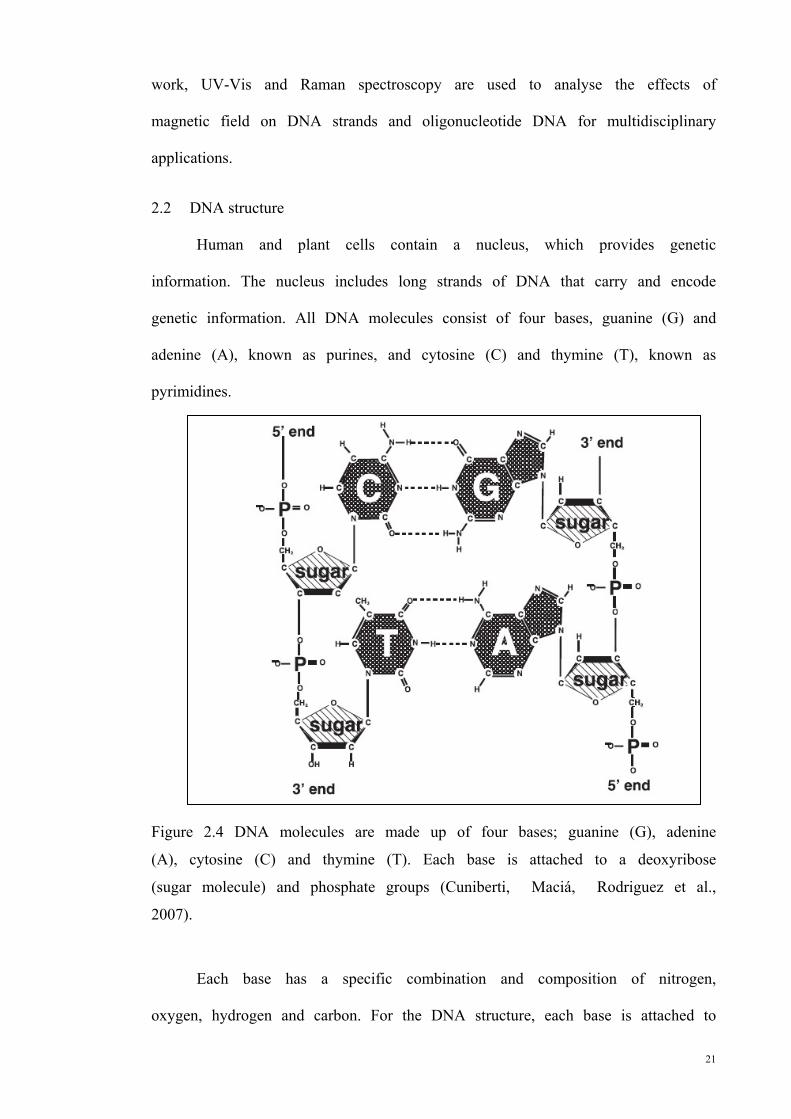
Figure 2.4 DNA molecules are made up of four bases; guanine (G), adenine (A),

cytosine (C) and thymine (T). Each base is attached to a deoxyribose (sugar molecule)

and phosphate groups (Cuniberti, Maciá, Rodriguez et al., 2007). ............................... 21

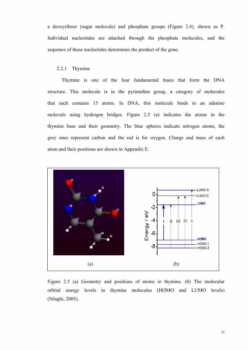
Figure 2.5 (a) Geometry and positions of atoms in thymine. (b) The molecular

orbital energy levels in thymine molecules (HOMO and LUMO levels) (Silaghi, 2005).

......................................................................................................................................... 22

Figure 2.6 The UV-Vis spectrum of thymine calculated using density functional

theory. ............................................................................................................................. 23

Figure 2.7 (a) Geometry and positions of atoms in cytosine. (b) The molecular

orbital energy levels in cytosine molecules (HOMO and LUMO levels) (Silaghi, 2005).

......................................................................................................................................... 24

Figure 2.8 The UV-Vis spectrum of cytosine calculated using density functional

theory. ............................................................................................................................. 24

xvii

Figure 2.9 (a) Geometry and positions of atoms in adenine. (b) The molecular

orbital energy levels in adenine molecules (HOMO and LUMO levels) (Silaghi, 2005).

......................................................................................................................................... 25

Figure 2.10 The UV-Vis spectrum of adenine calculated using density functional

theory. ............................................................................................................................. 26

Figure 2.11 (a) Geometry and positions of atoms in guanine. (b) The molecular

orbital energy levels in guanine molecules (HOMO and LUMO levels) (Silaghi, 2005).

......................................................................................................................................... 27

Figure 2.12 The UV-Vis spectrum of guanine calculated using density functional

theory. ............................................................................................................................. 27

Figure 2.13 DNA and nucleophile hydroxide interaction. A hydroxide or

activating water promotes the phosphate group by attaching to and splitting the DNA

strain (viewing the picture from left to right shows a schematic of the cleavage

mechanism). .................................................................................................................... 28

Figure 2.14 The cleavage of DNA by oxidation in the guanine site. ................. 29

Figure 2.15 The molecule with energy equal to ΔE, differences between the

HOMO-LUMO levels (energy gap). ............................................................................... 30

Figure 2.16 The angular momentum vector, L, can lie along specific orientations

with respect to the external magnetic field. .................................................................... 38

Figure 2.17 An atom is placed in a magnetic field with the convention that the

South Pole is at the top and the North Pole is at the bottom. .......................................... 38

Figure 2.18 The difference in energy between adjacent levels ............................ 39

Figure 2.19 The splitting of the sodium D line when the amplitude of the

magnetic fields increase from low to high shows this effect. ......................................... 42

Figure 2.20 Raman scattering mechanism, including Stokes, anti-Stokes and

Rayleigh scattering. ......................................................................................................... 44

xviii

Figure 3.1 An image of Mimosa pudica commonly known as the sensitive plant.

......................................................................................................................................... 47

Figure 3.2 DNA extraction protocol .................................................................... 48

Figure 3.3 Mask designed using AutoCAD 14 software. The left one is for the

negative photoresist while the right one is for the positive photoresist. ......................... 51

Figure 3.4 Patterns fabricated using positive and negative photoresists, positive

(left) and negative (right) ................................................................................................ 52

Figure 3.5 Schematic of the patterning mechanism. ........................................... 54

Figure 3.6 Procedure used to make a layer of SU-8 photoresist on a prepared

substrate. ......................................................................................................................... 54

Figure 3.7 Deposition techniques; chemical and physical processes. ................. 60

Figure 3.8 Thermal evaporation machine, belonging to the Department of

Physics, University of Malaya, used in the present study. .............................................. 61

Figure 3.9 A side view of the magnetic field generator used in this work. Two

coils are located parallel to each other and separated by a small distance. ..................... 62

Figure 3.10 Magnetic field generated via current in the magnetic generator in

various gap size between two coil pair (Helmholtz coil pair system)............................. 63

Figure 3.11 Measurement set up, including AVO meter, Tesla meter, timer,

thermometer , magnetic generator that included power supply and electromagnet and

wire connections . ......................................................................................................... 65

Figure 3.12 Diluted DNA sample placed in the magnetic field region (a)

Electromagnet; (b) Thermometer; (c) Multimeter; (d) Timer; (e) Teslameter; (f)

Electromagnet power supply and (g) DNA sample. ....................................................... 65

Figure 4.1 Flow-chart showing the two perspectives of analyses done in this

work based on the biological and Physics aspects. ......................................................... 67

xix

Figure 4.2 UV-Vis spectra of diluted AT-100 DNA sample after exposure to

magnetic fields of various strengths (250, 500, 750 and 1000 mT). ............................... 70

Figure 4.3 UV-Vis spectrum of diluted CG-100 DNA sample after exposure to

magnetic fields of various strengths (250, 500, 750 and 1000 mT). ............................... 70

Figure 4.4 UV-Vis spectrum of diluted P-DNA sample after exposure to

magnetic fields of various strengths (250, 500, 750 and 1000 mT) ............................... 71

Figure 4.5 The measurement setup included a magnetic field generator for

applying a uniform magnetic field, a thermometer to control and monitor the

temperature and an AVO meter to calculate the resistance. A drop of diluted DNA

placed between two metal electrode. .............................................................................. 71

Figure 4.6 The variation in the purity of diluted DNA samples (P-DNA, AT-100

and CG-100) against the magnitude of magnetic field strengths. ................................... 72

Figure 4.7 UV-Vis Spectrum for four different concentrations. Subfigure shows

the optical density versus concentration for the AT-100 oligonucleotide DNA. ............ 76

Figure 4.8 UV-Vis Spectrum for four different concentrations. The subfigure

shows the optical density versus concentration for CG-100 oligonucleotide DNA. ...... 77

Figure 4.9 UV-Vis absorption at various wavelengths and four different

concentrations. The subfigure shows the optical density versus concentration for the P-

DNA. ............................................................................................................................... 77

Figure 4.10 The variation in the extinction coefficients of diluted DNA exposed

to magnetic fields. ........................................................................................................... 79

Figure 4.11 Mechanism of the hydrolysis interaction in the DNA helix. ............ 80

Figure 4.12 Variation of the maximum wavelength in the absorption spectra of

diluted DNA influenced by magnetic field exposure. ..................................................... 82

Figure 4.13 Variation in the optical density of dilute DNA that was exposed to

magnetic fields. ............................................................................................................... 83

xx

Figure 5.1 The absorption spectra of diluted AT-DNA exposed to magnetic field

fitted by the equations for direct band gap transitions. ................................................... 87

Figure 5.2 The absorption spectra of diluted CG-DNA exposed to magnetic field

fitted by the equations for direct band gap transitions. ................................................... 88

Figure 5.3 The absorption spectra of diluted P-DNA exposed to a magnetic field

were fitted by the equations for direct band gap transitions. .......................................... 88

Figure 5.4 Kubelka-Munk coefficients of the absorption spectra of AT-DNA

exposed to various magnetic fields. ................................................................................ 89

Figure 5.5 Kubelka-Munk coefficients of the absorption spectra of CG-DNA


Figure 5.6 Kubelka-Munk coefficients of the absorption spectra of P-DNA


Figure 5.7 Dispersion curves of real part of the refractive index of AT-100 DNA

after exposure to different strengths of magnetic fields. ................................................. 94

Figure 5.8 Dispersion curves of real part of the refractive index of CG-100 DNA

after exposure to different strengths of magnetic fields. ................................................. 94

Figure 5.9 Dispersion curves of real part of the refractive index of P-DNA after

exposure to different strengths of magnetic fields. ......................................................... 95

Figure 5.10 Imaginary part of the refractive index of AT-100 DNA exposed to

magnetic fields. ............................................................................................................... 96

Figure 5.11 Imaginary part of the refractive index of CG-100 DNA exposed to

magnetic fields. ............................................................................................................... 97

Figure 5.12 Imaginary part of the refractive index of P-DNA exposed to

magnetic fields. ............................................................................................................... 97

Figure 5.13 Loss function of AT-100 DNA exposed to different magnetic field

strengths. ......................................................................................................................... 99

xxi

Figure 5.14 Loss function of CG-100 DNA exposed to different magnetic field

strengths. ......................................................................................................................... 99

Figure 5.15 Loss function of P-DNA exposed to different magnetic field

strengths. ....................................................................................................................... 100

Figure 5.16 Comparison of the Raman spectra of AT-DNA before and after

exposure to magnetic field. ........................................................................................... 102

Figure 5.17 Comparison of the Raman spectra of CG-DNA before and after


Figure 5.18 Comparison of the Raman spectra of P-DNA before and after


Figure 5.19 Resistivity of AT-DNA exposed to magnetic fields. ..................... 106

Figure 5.20 Resistivity of CG-DNA exposed to magnetic fields. ..................... 106

Figure 5.21 Resistivity of P-DNA exposed to magnetic fields.......................... 106

Figure 5.22 Temperature of AT-DNA exposed to magnetic fields. .................. 110

Figure 5.23 Temperature of CG-DNA exposed to magnetic fields. .................. 111

Figure 5.24 Temperature of P-DNA exposed to magnetic fields. ..................... 111

Figure 6.1 Potential applications of DNA strands and oligonucleotides in Physics

and Biology ................................................................................................................... 117

Figure 7.1 Two fluxes which are completely diffuse. One in the positive x-

direction, J, and one in the negative x-direction, I. ....................................................... 122

xxii

List of Abbreviations

A Adenine

AFM Atomic Force Microscopy

CVD Chemical Vapor Deposition

I–V Current-Voltage

C Cytosine

DFT Density Functional Theory

DNA Deoxyribonucleic Acid

DC Direct Current

dsDNA Double Stranded DNA

EF Fermi Level

FTIR Fourier Transform Infrared

G Guanine

HOMO Highest Occupied Molecular Orbital

IR Infrared

K-K Kramerz-Kroning

K-M Kubelka-Munk

LB Lambert-Beer

LUMO Lowest Unoccupied Molecular Orbital

MDM Metal-DNA-Metal MEMS Micro-Electro Mechanical Systems

MO Molecular Orbital

PVD Physical Vapor Deposition

PECVD Plasma Enhanced Chemical Vapor

PCR Polymerase Chain Reaction

RF Radio Frequency

SEM Scanning Electron Microscopy

ssDNA Single Stranded DNA

T Thymine

UV Ultraviolet

UV-Vis Ultraviolet-Visible

xxiii

List of Symbols

A Absorption.

σ* Anti bonding Molecular Orbital

A Average cross-section

Eg Band gap

k Boltzmann's constant

σ Bonding Molecular Orbital

Complex optical refractive index -

Complex optical refractive index- phase

C Concentration

σ Conductivity

I Current

J Current density

Dielectric Constant

m* Effective mass

FE Electric force

q Electron charge

ε Extinction Coefficient

EF Fermi Level

Imaginary dielectric constant

Imaginary part of Refractive index

L Length of the DNA

B Magnetic field

FB Magnetic force

O.P Optical Density

L Path length

H Planck's constants

K Propagation vector

Real part of dielectric constant

Real part of Refractive index Refractive index

R Resistance

T Temperature

V Velocity

~n

k~

)(ωε

ε ′′

in

ε′

rnn

xxiv

C Velocity of an electromagnetic wave

c0 Velocity of an electromagnetic wave in

Wave length

λ

1

1.1 CHAPTER I: INTRODUCTION

1.1 Introduction

In recent years, a lot of work has been conducted based on the use of

biological specimens such as deoxyribonucleic acid (DNA), a low-dimensional

form of nanomaterial for potential applications in photonics and electronics

devices. Investigations related to the effects of various environmental

conditions on DNA have been actively pursued in multidisciplinary studies due

to its potential applications in the biomedical and electronics fields. This field

of research is in its infancy with respect to potential applications in Physics and

electronics. Most recent research on this aspect in the field of Physics has been

focused on trapping and manipulating of DNA for use in biosensors and chips.

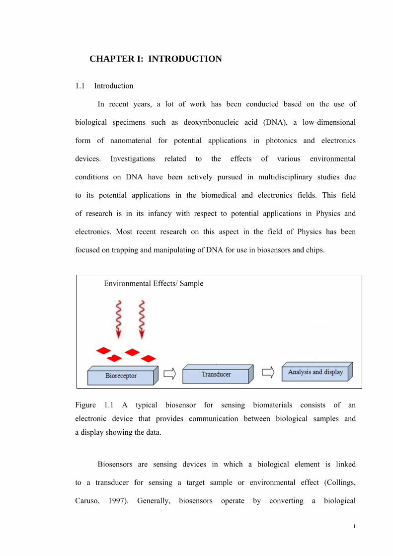
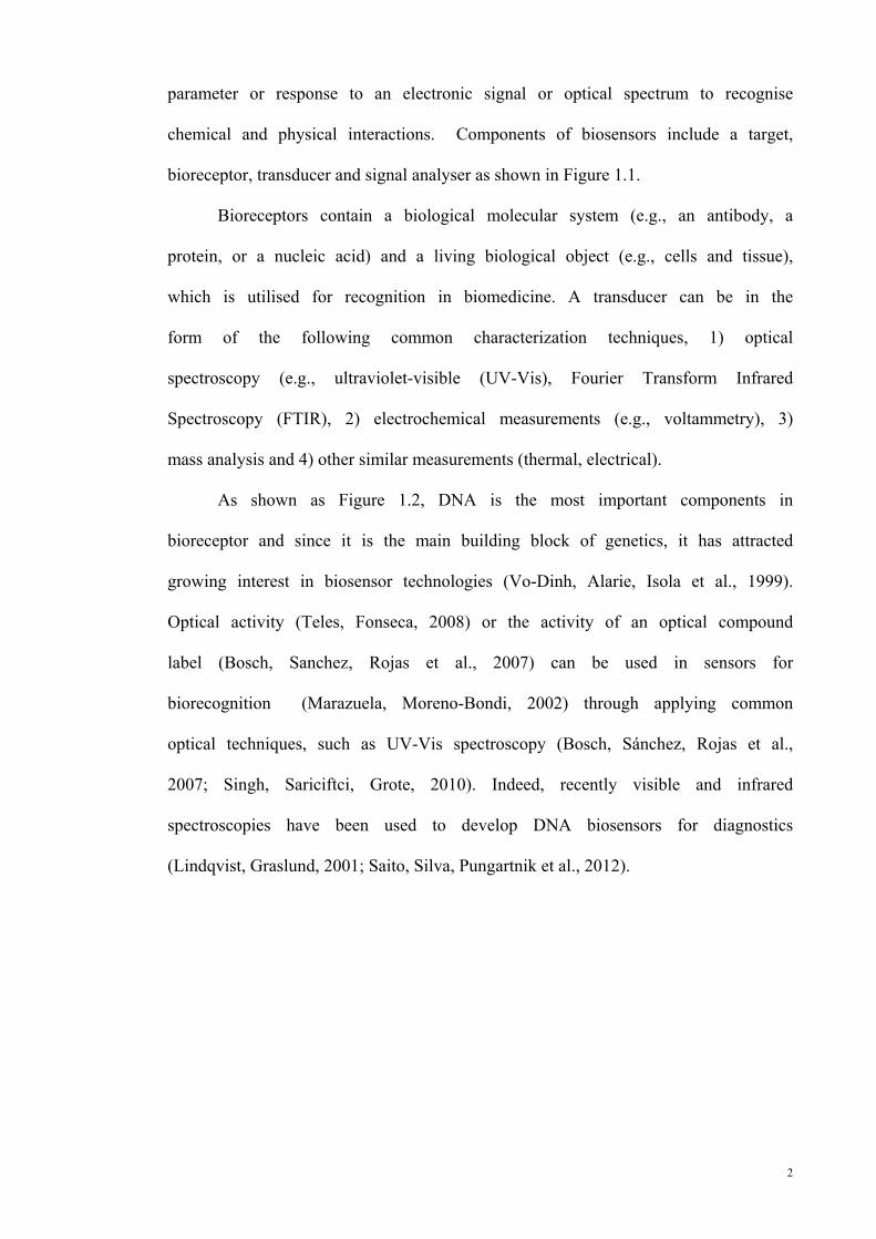
Figure 1.1 A typical biosensor for sensing biomaterials consists of an

electronic device that provides communication between biological samples and

a display showing the data.

Biosensors are sensing devices in which a biological element is linked

to a transducer for sensing a target sample or environmental effect (Collings,

Caruso, 1997). Generally, biosensors operate by converting a biological

Environmental Effects/ Sample

2

parameter or response to an electronic signal or optical spectrum to recognise

chemical and physical interactions. Components of biosensors include a target,

bioreceptor, transducer and signal analyser as shown in Figure 1.1.

Bioreceptors contain a biological molecular system (e.g., an antibody, a

protein, or a nucleic acid) and a living biological object (e.g., cells and tissue),

which is utilised for recognition in biomedicine. A transducer can be in the

form of the following common characterization techniques, 1) optical

spectroscopy (e.g., ultraviolet-visible (UV-Vis), Fourier Transform Infrared

Spectroscopy (FTIR), 2) electrochemical measurements (e.g., voltammetry), 3)

mass analysis and 4) other similar measurements (thermal, electrical).

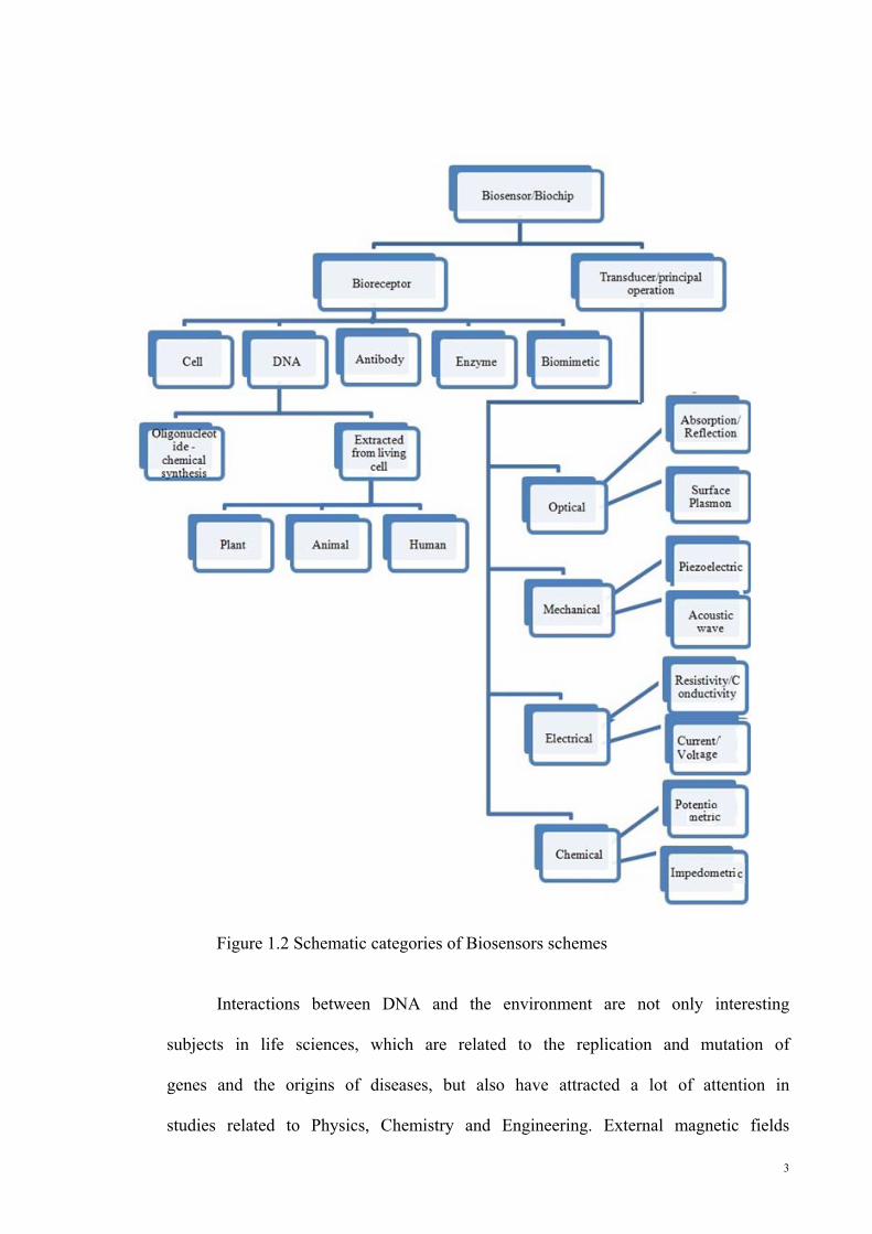
As shown as Figure 1.2, DNA is the most important components in

bioreceptor and since it is the main building block of genetics, it has attracted

growing interest in biosensor technologies (Vo-Dinh, Alarie, Isola et al., 1999).

Optical activity (Teles, Fonseca, 2008) or the activity of an optical compound

label (Bosch, Sanchez, Rojas et al., 2007) can be used in sensors for

biorecognition (Marazuela, Moreno-Bondi, 2002) through applying common

optical techniques, such as UV-Vis spectroscopy (Bosch, Sánchez, Rojas et al.,

2007; Singh, Sariciftci, Grote, 2010). Indeed, recently visible and infrared

spectroscopies have been used to develop DNA biosensors for diagnostics

(Lindqvist, Graslund, 2001; Saito, Silva, Pungartnik et al., 2012).

3

Figure 1.2 Schematic categories of Biosensors schemes

Interactions between DNA and the environment are not only interesting

subjects in life sciences, which are related to the replication and mutation of

genes and the origins of diseases, but also have attracted a lot of attention in

studies related to Physics, Chemistry and Engineering. External magnetic fields

4

can be useful tools for manipulating and controlling material and

physiochemical interactions remotely. The more interesting question is whether

static magnetic fields can cause damage to DNA structure and alter its optical

properties. There are many studies focused on this issue. Magnetic field can

result in changes in the energy levels and thus causes movement of charges in

DNA molecules and can have influence on the DNA responsiveness. Also, by

controlling and manipulating the magnetic field remotely, this effect can be

used to extend its application in the medical and biosensors area. As result of

this, the effects of magnetic field exposure on biomaterials have gained a lot of

attention in recent years in research. Biomaterials can be easily manipulated

using an external magnetic field. For instance, magnetic particles that are

tagged to a biomaterial can be made to move or stretch using magnetic force

and magnetic treatments can be applied to tissue and blood (Dobson, 2008;

Strick, Allemand, Bensimon et al., 1996). In the biomaterials category in

general, the biological and scientific research interest in DNA strand

manipulation using moderate-intensity magnetic fields has increased.

Interesting studies involve immobilised DNA strands on small chips,

mechanically manipulated DNA in a magnetic tweezers device (Haber, Wirtz,

2000) and magnetically arranged DNA in liquid crystals (Brandes, Kearns,

1986; Davidson, Strzelecka, Rill, 1988). Another interesting application,

reported by our group, involves magnetic sensors in metal-DNA-metal

structures (Khatir, Banihashemian, Periasamy, Ritikos, Abd Majid et al.,

2012). Feasible electrical and medical applications of applying magnetic fields

to DNA provided new perspectives for DNA manipulation and

characterisations (Lan, Chen, Chang, 2011).

5

The in vivo effect of magnetic fields on DNA in rat brains was

previously studied (Lai, Singh, 2004). However, in this work the effect of

magnetic fields on DNA in vitro using an optical method is investigated for the

first time.

In this work, spectroscopic characterizations of diluted DNA

oligonucleotides AT (100mer) and CG (100mer) and DNA extracted from

plant subjected to an external magnetic field are conducted using UV-Vis

spectroscopy to determine their potential for use in electronic devices and

biosensor applications. The optical spectra of the DNA are measured to study

the optical parameter such as refractive index and band gap with respect to the

strength of the applied magnetic field.

1.2 Motivations

Biosensors are powerful tools for identifying toxic compounds in

industrial products, biological samples (e.g., virus, tissue and bacteria) and

environmental systems (e.g., water). The effects of environmental pollution can

be recognized and detected by applying optical and electrical detection tools to

biological samples. The simplicity, speed, high selectivity and sensitivity in

using the small geometry of biomaterial based micro- and nanochips for

detecting molecules and environmental interactions make biomaterials as the

current preferred tools for researchers in detectors.

DNA strands and short oligonucleotides with several tens of base pairs

in large group of biomaterials are novel candidates for biochips and sensors

because of their unique properties which can result in DNA-based sensing

devices. The interest in hybrid structures of biomaterials and electronic

elements (metal/semiconductor, biomaterial/DNA) has increased tremendously

6

recently (Braun, Eichen, Sivan et al., 1998; Richter, Mertig, Pompe et al.,

2001).

Practical use of DNA and bio-components in micro- and

nanoelectronics as sensors, including magnetic and opto-magnetic detectors

has significantly created great interest in the investigation of magnetic field

effects on DNA and short-length oligonucleotides. In this work, the optical

absorption of diluted DNA exposed to external magnetic fields is investigated

from the optical density measurements. The main purpose of this study is to

investigate the possibility of using the effects of magnetic fields on DNA for

medical and industrial applications. The possible applications include magnetic

sensors, biochips, microfluidic devices, nanoparticle separation and virus

detection.

1.3 Objectives

The main objectives of this study are measured from the analysis done

on the results obtained from the optical and physical properties of DNA

extracted from plants (Mimosa pudica) as a natural DNA that was available in

our living area and of oligonucleotide DNA as a simplest artifitual DNA , after

exposure to different magnetic field strength. All measurements are performed

before and after exposure to the magnetic field and analysed from the

biological as well as the physical perspectives. The objectives of the work done

in this research are highlighted below.

1. To determine the effects of exposure of DNA samples to different

magnetic field strength from the biological perspective on the following

parameters:

(i) DNA purity

(ii) The extinction coefficient of DNA

7

(iii) The optical density of DNA.

(iv) The wavelength of the DNA absorption peak.

2. To determine the effects of exposure of DNA samples to different

magnetic field strength from the physics perspective on the following

parameters:

(i) Band gap of DNA samples

(ii) Refractive index of DNA samples

(iii) The hydrogen bonds in the DNA helix.

(iv) The resistivity of DNA samples.

(v) DNA temperature variations.

(vi) The loss function of DNA samples.

3. To explain the effects of exposure to in vitro magnetic field on the

above parameters both from the biological and physics perspective in

relation to the structure of DNA.

1.4 Thesis outline

The thesis is organized into 6 chapters. Chapter I begin with a brief

introduction on biosensors and the classification of biosensors. Importance of

studies related to biosensors and magnetic field influence on DNA is also

highlighted. The research problems and significance of the studies are

discussed, including the study features, analysis conditions and limitations.

Aims and motivations of the work are presented and the objectives are outlined

in this chapter.

Chapter II provides an organised literature review covering the various

concepts used in this study. The highlighted studies featured in this review are

8

related to the objectives of this study. The theoretical background of this work

is presented, discussed and categorised.

Chapter III describes the research methodology adopted in this work for

data collection and processing. The materials, instruments and devices used in

carrying out the research are described in the first part of the chapter followed

by the fabrication process, extraction methods and analysis. Limitations and

problems of the analysis are briefly mentioned in the final parts of this chapter.

Chapter IV presents the results with discussions and analysis of the data

based on the biological aspects. The data analysis and calculation techniques

are also described in this chapter. Similarly the results with discussions and

analysis of the data based on the physics aspect are presented in Chapter V. In

both these chapters, analysis of the data are presented in diagrams, charts and

tables obtained from scientific software, such as Microsoft Excel, SPSS and

ADF, The results are discussed using physical and chemical principles to relate

the effects of magnetic field strength on the various parameters studied in this

work and the accuracy of the hypothesis investigated.

Finally, Chapter VI presents the conclusions and recommendations for

future works.

….

.

.

.

.

9

2.1 CHAPTER II: REVIEW OF RELATED LITERATURE

2.1 Introduction

The effects of exposing biomaterials to magnetic fields have gained

considerable attention in the past several decades. Biomaterials can be easily

manipulated by an external magnetic field. Magnetic particles that are tagged

to biomaterials for instance, can be moved and stretched using magnetic force

(Chen, Fu, Zhu et al., 2011) and can be treated using magnetic fields (Elson,

2009). Magnetic fields can also be used to manipulate tissue and blood (blood

cell separation using Magnetophoresis). As part of the general biomaterials

category, biological and scientific research in manipulating DNA strands using

moderate-intensity magnetic fields has increased. Immobilising DNA strands

on small chips (Campàs and Katakis, 2004), mechanically manipulating DNA

using a magnetic field in a magnetic tweezer device (Brogioli, 2009; Leuba,

Wheeler, Cheng et al., 2009) and magnetically arranging liquid crystals (Morii,

Kido, Suzuki et al., 2004) have been reported. Magnetic sensors in metal-

DNA-metal structures are another interesting application reported by our group

(Khatir, Banihashemian, Periasamy, Abd Majid et al., 2012) .

To investigate the interest in magnetic fields and DNA, statistical

analysis was performed using a database. The subjects that were published in

this field were investigated by categorising the published papers by the type of

document, the subject area and the number of papers. The pie chart in Figure

2.1 depicts the number of papers in the respective subjects. As depicted in this

figure, 37.8% of the published papers and conference proceedings are from the

Physics perspective, 17.2% are related to Engineering and 12.2% are in the

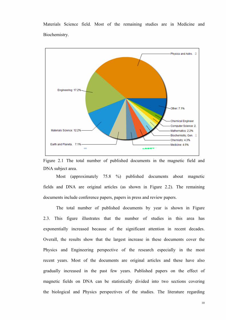
10

Materials Science field. Most of the remaining studies are in Medicine and

Biochemistry.

Figure 2.1 The total number of published documents in the magnetic field and

DNA subject area.

Most (approximately 75.8 %) published documents about magnetic

fields and DNA are original articles (as shown in Figure 2.2). The remaining

documents include conference papers, papers in press and review papers.

The total number of published documents by year is shown in Figure

2.3. This figure illustrates that the number of studies in this area has

exponentially increased because of the significant attention in recent decades.

Overall, the results show that the largest increase in these documents cover the

Physics and Engineering perspective of the research especially in the most

recent years. Most of the documents are original articles and these have also

gradually increased in the past few years. Published papers on the effect of

magnetic fields on DNA can be statistically divided into two sections covering

the biological and Physics perspectives of the studies. The literature regarding

11

the effects of static magnetic fields on DNA strands from biological and

physical perspectives is reviewed by considering the application and

characterisation methods.

Figure 2.2 Published documents on DNA and magnetic fields according to

categories.

Figure 2.3 The total number, by year, of published documents about DNA and

magnetic fields.

0

4000

8000

12000

16000

20000

24000

1908 1928 1948 1968 1988 2008

Num

ber

of d

ocum

ents

Year

12

2.1.1 Biological perspective

Effect of magnetic fields on biomaterials and living cells is an

interesting subject with numerous publications since more than 50 years. The

more interesting question is whether static magnetic fields cause damage to

DNA structure and alter its properties. There are many studies focusing on this

issue. It has been reported that 50/60 Hz magnetic fields increase the damage

via the effect on trace amounts of ions in cells (Jajte, ZmyÅ›lony, Palus et al.,

2001; McNamee, Bellier, McLean et al., 2002). Strong static magnetic field

can affect gene expression and charge transportation (Kimura, Takahashi,

Suzuki et al., 2008). Furthermore, magnetic treatments have been reported in

the treatment of Ehrlich carcinoma (El-Bialy and Rageh, 2013). The published

papers on magnetic field effects on DNA are listed and categorized in Table 2-

1. As shown in the table, one of the earliest studies on the effect of magnetic

fields on a biological sample was performed by Barnothy in 1964 (Barnothy,

1964). Fox published similar research in 1966 (Fox, 1966) and many papers on

this topic were published afterwards (Bodega, Forcada, Suárez et al., 2005;

Eldashev, Shchegolev, Surma et al., 2010;Kirschvink, Kobayashi-Kirschvink

Woodford, 1992; Leszczynski, 2005; Miyakoshi, 2006; Moore, 1979; Sekino,

Tatsuoka, Yamaguchi et al., 2006). The broad range of studies on biomaterials

and magnetic fields provided new applications in medicine. These includes

treatment in muscle cells (Eldashev et al., 2010), cancer therapy (Raylman,

Clavo Wahl, 1996), brain research, diseases (e.g., Parkinson's and Alzheimer's)

(Ueno, 2012), magnetic resonance imaging (MRI) measurements of brain

impedance (Leszczynski, 2005; Sakurai, Terashima Miyakoshi, 2009) and the

control and growth of cells (Lucia Potenza, Ubaldi, De Sanctis et al., 2004),

including those in specific orientations (Morii, Kido et al., 2005). The effects

13

of magnetic fields on DNA are more interesting than the effects of electric

fields’ because of the specific change in properties and roles of DNA in cells

when exposed to magnetic field.

Published works addresses the in vivo magnetic field effects on DNA

(Ichioka, Minegishi, Iwasaka et al., 2000) and in vitro (Blackman, Benane,

Rabinowitz et al., 1985). Some of the research showed that high magnetic field

exposure damages living cells in vivo. For instance, in rat brain, free radicals

that are found in biological organisms created by magnetic fields damage the

brain (Amara, Douki, Garrel et al., 2011; Lee, Johng, Lim et al., 2004; Pan and

Liu, 2004; Theodosiou and Thomas, 2008; Villarini, Moretti, Scassellati-

Sforzolini et al., 2006) showed cleaved double-stranded DNA (Kim, Ha, Lee et

al., 2010). Studies about the effects of magnetic fields on DNA in vitro show

reorientation of DNA in the direction of the magnetic field (Emura, Ashida,

Higashi et al., 2001; Gamboa, Gutiérrez, Alcalde et al., 2007). Improvements

in magnetic configurations also permit magnetic sorting, stretching and

twisting of DNA strands using small volumes of biomaterial and various

bioapplications (Al-Hetlani, Hatt, Vojtíšek et al., 2010; Thachappillya

Mukundan, Tran Tuona Phan, 2013).

Various applications of magnetic field effects on DNA that have been

reported are organised in Tables 2-1 and 2-2. The overwhelming majority of

these researches were performed in vivo.

14

Table 2-1 Published papers on work related to magnetic fields and DNA shown

chronologically by year and the applications based on the biological

perspective.

Authors

Year

PCR

Magnetic

bead

Micro fluid,

Chanel

Drug

and treatm

ent

Separation, orientation

Deviation,

Dam

age

in vivo

Barnothy and et al 1969 * * Fox, M. A. 1966 * Moore, R. L. 1979 * * Ueno, S. 1992 * * Lin H and et al 1995 * * Zannella, S. 1998 * * Emura R., and et al 2001 * Jandova A and et al 2001 * Curcio M and et al 2002 * * Saunders, R. D. 2002 * * Hautot D and et al 2003 * * Codina A. and et al 2004 * * * Laing T.D. and et al 2004 * Morii N. and et al 2004 * Woldansk and et al 2004 * * Wen J and et al 2004 * Pan H and et al 2004 * * Morii N and et al 2005 * * Gamboa O.L and et al 2007 * * Ohashi T and et al 2008 * * * * Theodosiou E and et al 2008 * * * Kimura T and et al 2008 * * * Roberts C and et al 2008 * Lhuillier S and et al 2009 * * Elson E. 2009 * * Sakurai T and et al 2009 * Elson E. 2009 * * Boles D.J and et al 2011 * * * * Higashi T and et al 2011 * Pozhidaeva and et al 2012 * * * Cannon B and et al 2012 * Lim J and et al 2012 * * El-Bialy N.S and et al 2013 * *

15

Of the wide range of analysis methods used in biological sciences to

trace the variation, damage and interaction of DNA, UV-Vis spectroscopy is

one of the most convenient and commonly used tools. Zai et al. in 1998

published research about the DNA and protein constituents of viruses that were

characterised using UV-Vis spectroscopy (Zai Qing and Thomas G.J, 1998).

Toyama et al. in 2001, reported the use of UV-Vis spectroscopy to analyse

adenine residues in DNA (Toyama, Miyagawa, Yoshimura et al., 2001). In

2005, Zhou and co-researchers studied the interaction between CT-DNA and

cytochrome C using electrochemistry and UV-Vis spectroscopy (Zhou, Feng,

Wu et al., 2005). DNA that was functionalised by nanoparticles of gold was

investigated using UV-Vis spectroscopy in the Witten research group (Witten,

Bretschneider, Eckert et al., 2008).

Drug-DNA interactions are another subject that can be studied using

UV-Vis analysis (Perveen, Qureshi, Ansari et al., 2011). Raman spectroscopy

is another technique for analysing biomaterials and their interaction with other

materials or the environment. Although this method is not as widely used as

UV-Vis spectroscopy, Raman is a useful method for analysis in

multidisciplinary studies. In 1999, Yiming X. et al. studied the microscopic

damage of DNA using Raman spectroscopy (Yiming, Zhixiang, Hongying et

al., 1999). In 2001, Ke et al. investigated the microscopic DNA damage caused

by acetic acid using Raman spectroscopy (Ke, Yu, Gu et al., 2001). Shaw C.P.

and Mallidis C. studied damaged DNA structures (Mallidis, Wistuba,

Bleisteiner et al., 2011; Shaw C.P and Jirasek, 2009). Human sperm damage

also can be investigated using Raman spectroscopy tools (Niederberger, 2012,

2013). Combining Raman and UV-Vis spectroscopy is a powerful tool that

16

provides complementary results using the parallel analysis techniques (Jangir,

Dey, Kundu et al., 2012; Kang and Zhou, 2012).

2.1.2 Physics perspective

The influence of magnetic fields on DNA is analysed to utilise this

material as a smart element in electronics. Lack of physical and industrial

studies of this material encourages us to investigate the capability of this smart

material by extending the monitoring of DNA variations. The application of

this structure as a multidisciplinary material is clearly a subject that compels

many scientists around the world to manipulate DNA structures.

This field of research is in its infancy in Physics and electronics. Most

recent research from a Physics perspective is focused on manipulating and

trapping DNA for its use as sensors and on chips. Combining nanoparticles

with DNA molecules extends the capability of this material.

Piunno P.A.E. and his research group in 1999 published one of the first

papers in which DNA was introduced to engineering. The researchers

immobilised DNA using fibre optics (Piunno, Watterson, Wust et al., 1999). In

the same year, several studies were published using DNA and oligonucleotide

biosensors and by optimising parameters, such as immobilisation and

hybridisation (Liu and Tan, 1999; Xu, Ma, Liu et al., 1999; Zhang, Zhou,

Yuan et al., 1999). The original article in 2000 showing the use of DNA in

sensors, such as those in fibre optics and piezoelectricity, attracted significant

attention (Mehrvar, Bis, Scharer et al., 2000; Piunno, Hanafi-Bagby, Henke et

al., 2000; K. R. Rogers, 2000; Tombelli, Mascini, Sacco et al., 2000; Walt,

2000; Wolfbeis, 2000). In 2001, Lin et al. published a review of fibre-optic

DNA biosensors as a new developing technology that has high potential for

detecting oligonucleotide patterns, diagnosing gene or DNA damage, and

17

identifying drugs and enzymes using fibre optics sensors (Lin and Jiang, 2001).

The number of papers describing DNA applications in biosensors and fibre-

optic sensors increased significantly since 2001 (Ahmad, Chang, King et al.,

2005; Epstein, BiranWalt, 2002; Jiang, LeiGao, 2006; Martins, Prazeres,

Fonseca et al., 2010; Peter, Meusel, Grawe et al., 2001; Kim R Rogers,

Apostol, Madsen et al., 2001).

Table 2-2 Published papers about magnetic fields and DNA by year and

application from a Physics perspective.

Authors YearNano/

MicroparticleChip/ Sensor Separation Tweezers

Sonti, et al 1997 * Iwasaka et al 1998 * * Iwasaka, et al 1998 * Yan J et al 2004 * * * Morii, N. et al 2004 * Graham D.L et al 2005 Mykhaylyk, et al 2007 * Klaue D et al 2009 * Leuba, S. H. et al 2009 * * * Peng, H. et al 2009 * * Brogioli, D. 2009 *

Manosas, M. et al 2010 * Chan, et al 2011 * Khatir et al 2012 * * Lionnet, T. et al 2012 * Lim, J.Dobson, J. 2012 * Chen, H. et al 2012 * Mahmoudy et al 2012 * Medley, C. D. et al 2012 * De Vlaminck, I. et al 2013 *

Tables 2-1 and 2-2, shows that the number of papers published about

the interaction between magnetic fields and DNA from a biological perspective

is greater than that for the physical perspective. Most of the researches from

the Physics perspective were performed in the past few years, indicating that

18

the research in this subject is still in its infancy. Recently, DNA strand

manipulation and measurements in the presence of magnetic fields have

attracted significant scientific research attention. Magnetic tweezers are used to

study and manipulate individual DNA strands using a combination of magnetic

fields and a microscope.

In 2004, Potenza L. et al. investigated the effects of a large static

magnetic field on various DNA molecules in vivo and in vitro. The researchers

analysed the magnetic field effect from a biological perspective. Their results

showed that in vitro magnetic fields induce DNA mutations and that exposure

to large magnetic fields perturbs the stability of DNA. However in vivo, this

effect is not serious because of cellular protection (L. Potenza, Cucchiarini,

Piatti et al., 2004).

As shown in Table 2-2, the number of studies that were performed

using magnetic field as tweezer-like tools to control DNA has increased. In

2004, Yan et al. studied and manipulated single DNA molecules using

magnetic fields (Static fields, 2 006). In 2009, the research groups of Brogioli,

Peng and Leuba separately released their results about using magnetic fields to

control single DNA molecules (Peng and Ling, 2009). In 2010, Manosas, M. et

al reported DNA tracking motors (Manosas, Meglio, Spiering et al., 2010). In

2012, Lionnet, T. et al reported using magnetic fields to trap a single DNA

molecule (Lionnet, Allemand, Revyakin et al., 2012). All of this research

focused on controlling DNA by using magnetic fields to capture and

manipulate DNA to extend its application without limiting or altering its

physical properties.

Using magnetic field is advantageous not only in sensors and

manipulation but also in separating nanoparticles and ions. A magnetophoretic

19

force can separate ions and charged materials, including DNA and particles to

which DNA are attached. In 1998, Iwasaka et al. investigated the use of

magnetophoresis with macromolecules. The researchers studied proteins and

DNA using optical transmittance analysis in a high magnetic field (8 T

superconducting solenoid) (Iwasaka and Ueno, 1998).

Microfluidic-based approaches have been used to place specific types of

forces on linear nucleic acids of various lengths and motilities. The nucleic

acids are placed on a surface and are subjected to electrophoresis through

micron-sized obstacles. Magnetic tweezers (Salerno, Brogioli, Cassina et al.,

2010), microfluidics, molecular motors, and DNA-drug interactions are helping

investigations for manipulating the behaviour of a DNA strand using magnetic

fields and magnetic nanosized beads (Mosconi, Allemand, Bensimon et al.,

2009).

The latest studies, by our own group, reported the effect of magnetic

fields on DNA for use in sensors and chips (Khatir, Banihashemian,

Periasamy, et al., 2012; Khatir, Banihashemian, Periasamy, et al., 2012). DNA

deposited between metallic gaps was exposed to magnetic fields of various

intensities. The analysis was based on electrical characterisation and physical

parameters. In this thesis, previously unreported effects of magnetic fields on

DNA features, from both biological and physical perspectives are investigated.

The main purpose of this study is to investigate DNA in an external magnetic

field. This situation can be applied to sensors and chips for detecting and

distinguishing samples. Our reported work includes aspects of novel

multidisciplinary studies continuing previous studies. This work includes

additional studies of the potential of DNA as a sensor, specifically as a

magnetic sensor and as a light sensor, and investigates environmental effects

20

on DNA. In vitro characterisations of the influence of magnetic fields on DNA

strands are proposed, and these characterisations can be applied in Physics,

Biology, Medicine and electronic devices. Studying the optical parameters of

DNA molecules exposed to external magnetic fields, in both the general

research area and in this paper, is interesting. This study provides a simplified

physical picture of the effect of a magnetic field on DNA integrity in vitro. The

optical absorption of diluted DNA under external magnetic fields was

investigated by measuring the intensity of normally incident light that passes

through a transparent quartz cuvette. The absorption, purity and extinction

coefficient of DNA were measured using UV-Vis spectroscopy. To verify the

results, a micro-Raman spectrum with a surface-enhanced Raman signal on a

thin layer of Au was measured. Both the UV-Vis and Raman results indicate

breakage of the DNA strands. Manipulation of DNA strands by magnetic

fields is an interesting idea that has been suggested to be applied to DNA

bioassays, microfluidic manipulation and nanoparticle capture. In conclusion,

this research shows that these materials have potential in biomedical and

electronic devices and are indispensable tools in diagnostics tests. Optical

characteristics of DNA using UV-Vis spectroscopy are commonly studied in

Physics by calculating the optical constant and the band gap. The Kubelka-

Munk theory (Y. Yang, Celmer, Koutcher et al., 2002) and the Kramers-

Kronig function are used as mathematics tools to analyse the refractive index

and calculate the band gap (Pinchuk, 2004; Singh et al., 2010). Kramers-

Kronig function is a powerful tool for analysing the optical constant of DNA

(Houssier and Kuball, 1971; INAGAKI, Hamm, Arakawa et al., 1974). DNA

optical analysis also includes band gap calculations (Iguchi, 2001; Wang,

LewisSankey, 2004; Yousef, Abu El-Reash, El-Gammal et al., 2013). In this

21

work, UV-Vis and Raman spectroscopy are used to analyse the effects of

magnetic field on DNA strands and oligonucleotide DNA for multidisciplinary

applications.

2.2 DNA structure

Human and plant cells contain a nucleus, which provides genetic

information. The nucleus includes long strands of DNA that carry and encode

genetic information. All DNA molecules consist of four bases, guanine (G) and

adenine (A), known as purines, and cytosine (C) and thymine (T), known as

pyrimidines.

Figure 2.4 DNA molecules are made up of four bases; guanine (G), adenine

(A), cytosine (C) and thymine (T). Each base is attached to a deoxyribose

(sugar molecule) and phosphate groups (Cuniberti, Maciá, Rodriguez et al.,

2007).

Each base has a specific combination and composition of nitrogen,

oxygen, hydrogen and carbon. For the DNA structure, each base is attached to

22

a deoxyribose (sugar molecule) and phosphate groups (Figure 2.4), shown as P.

Individual nucleotides are attached through the phosphate molecules, and the

sequence of these nucleotides determines the product of the gene.

2.2.1 Thymine

Thymine is one of the four fundamental bases that form the DNA

structure. This molecule is in the pyrimidine group, a category of molecules

that each contains 15 atoms. In DNA, this molecule binds to an adenine

molecule using hydrogen bridges. Figure 2.5 (a) indicates the atoms in the

thymine base and their geometry. The blue spheres indicate nitrogen atoms, the

grey ones represent carbon and the red is for oxygen. Charge and mass of each

atom and their positions are shown in Appendix E.

Figure 2.5 (a) Geometry and positions of atoms in thymine. (b) The molecular

orbital energy levels in thymine molecules (HOMO and LUMO levels)

(Silaghi, 2005).

(a) (a) (b)

23

Figure 2.6 The UV-Vis spectrum of thymine calculated using density

functional theory.

Thymine molecules have a deviation from the plane, and the average of

deviation is approximately 0.320 Å. All atoms in thymine, except the hydrogen

atoms, are coplanar. Figure 2.5 (b) indicates the molecular orbital energy level

in thymine molecules (HOMO and LUMO levels). HOMO is represented as π,

and LUMO as π*. The arrows indicate the main electronic transitions. UV-Vis

spectrum of thymine calculated using density functional theory is shown in

Figure 2.6. As depicted in this figure, the maximum wavelength absorption

occurs near 260 nm.

2.2.2 Cytosine

Cytosine is another base found in DNA. This molecule is the smallest of

the four bases. Cytosine is a pyrimidine that contains 13 atoms, and a cytosine

can have a hydrogen bond to a guanine molecule.

24

Figure 2.7 (a) Geometry and positions of atoms in cytosine. (b) The molecular

orbital energy levels in cytosine molecules (HOMO and LUMO levels)

(Silaghi, 2005).

Figure 2.8 The UV-Vis spectrum of cytosine calculated using density

functional theory.

(a) (b)

25

Figure 2.7 (a) shows the atomic geometry and positions of cytosine. The

blue spheres indicate nitrogen atoms, the grey ones represent carbon and the

red is for oxygen. Deviation from planarity in cytosine is approximately 0.007

Å. Figure 2.7 (b) illustrates the molecular orbital energy levels in cytosine

molecules (HOMO and LUMO levels). The UV-Vis spectrum of cytosine

calculated using density functional theory is shown in Figure 2.8. As depicted

in this figure, the maximum absorption occurs at approximately 260 nm.

2.2.3 Adenine

Adenine meanwhile is a purine. Adenine and thymine form a hydrogen

bonds. The largest component, with 15 atoms, in a DNA helix is adenine.

Figure 2.9 (a) shows the molecular structure of adenine.

Figure 2.9 (a) Geometry and positions of atoms in adenine. (b) The molecular

orbital energy levels in adenine molecules (HOMO and LUMO levels)

(Silaghi, 2005).

In this base, there is no oxygen atom. The blue spheres indicate nitrogen atoms

and the grey ones represent carbon. Figure 2.9 (b) indicates the molecular

orbital energy levels in adenine (HOMO and LUMO levels). The UV-Vis

(a) (a) (b)

26

spectrum of adenine calculated using density functional theory is shown in

Figure 2.10. As depicted in this figure, the maximum absorption is at

approximately 252 nm.

Figure 2.10 The UV-Vis spectrum of adenine calculated using density

functional theory.

2.2.4 Guanine

Guanine, with 16 atoms in its molecular structure, is also a purine.

Guanine is the counterpart to cytosine, with which it forms hydrogen bonds.

The molecular structure of guanine is depicted in Figure 2.11 (a), in which the

blue spheres indicate nitrogen atoms and the grey ones represent carbon.

Figure 2.11 (b) indicates the molecular orbital energy levels in guanine. The

UV-Vis spectrum of guanine according to density functional theory is shown

in Figure 2.12. As depicted in this figure, the maximum absorption is

approximately 257 nm. A Cartesian depiction of the geometry of guanine

shows a deviation from the plane of the molecule of approximately 0.09 Å

(APPENDIX E).

27

Figure 2.11 (a) Geometry and positions of atoms in guanine. (b) The molecular

orbital energy levels in guanine molecules (HOMO and LUMO levels)

(Silaghi, 2005).

Figure 2.12 The UV-Vis spectrum of guanine calculated using density

functional theory.

(a) (b)

28

2.3 Types of DNA cleavage

DNA cleavage is an important process in all living cells. There are three

categories of DNA cleavage: DNA hydrolysis, photochemical cleavage and

oxidative cleavage. The last two types of cleavage are closely related.

2.3.1 DNA hydrolysis

The general mechanism of the DNA hydrolysis process is a type of

nucleophilic attack on the phosphate side of the DNA helix. Cleavage results in

the scission of either the 3’-PO or the 5’-PO.

Figure 2.13 DNA and nucleophile hydroxide interaction. A hydroxide or

activating water promotes the phosphate group by attaching to and splitting the

DNA strain (viewing the picture from left to right shows a schematic of the

cleavage mechanism).

Figure 2.13 indicates the mechanism of hydrolysis in the DNA helix. A

hydroxide or activating water acts as a nucleophile or activates the phosphate

group in a nucleophilic attack (left). Otherwise, the leaving group can depart.

In Double strand DNA(dsDNA), the overlap of the molecular orbitals in the

base pairs leads to a decrease and minimisation of the light intensity in UV

region. Indeed, the cleavage decreases the overlap and then increases the UV

absorbance.

29

2.3.2 Photochemical cleavage of DNA

DNA cleavage is a production of reactive species such as oxygen by

photochemical process. In photochemical and oxidative DNA cleavage, the

reduced oxygen species generate reactive intermediates (Dunn, Lin, Kochevar,

1992; Nielsen, Jeppesen, Egholm et al., 1988).

The DNA cleavage is because of the oxidation interaction in guanine

bases (Figure 2.14). Guanine has a low energy of ionization as compared to

rest of the bases. Ionization energy for adenine, cytosine, guanine and thymine

are 8.24, 8.87, 7.75 and 9.14, respectively (Slavicek, Winter, Faubel et al.,

2009; Yang, Wang, Vorpagel et al., 2004).

Figure 2.14 The cleavage of DNA by oxidation in the guanine site.

The excited site in DNA generates oxygen, which modifies guanine

base, in contrast to superoxide. Damage of DNA observed via this pathway

forms guanine radical cations which can then be utilized as a label or tag for

detection or attaching other materials.

2.4 UV-Vis spectroscopy

UV-Vis spectroscopy is the fundamental scheme of molecular orbitals.

Molecular orbitals can define all molecules by subtracting or adding atomic

orbitals made from bonding and antibonding levels. Highest Occupied

Molecular Orbital or HOMO is the bonding orbital that contains the valence

electrons. The Lowest Occupied Molecular Orbital (LOMO) is known as

bonding orbital that is normally devoid of electrons. This description is valid

30

for single molecules. In bulk materials that include many atoms, the addition of

individual atomic orbitals form closely spaced orbitals, known as bands.


Interaction between electromagnetic wave and molecules cause the

atoms to undergo vibration; the higher the energy, the shorter the wavelength.

The energy of radiation in the UV (200-400 nm) and visible (400-700 nm)

range causes transitions between electronic levels in organic materials.

Molecular orbital in organic materials consists of one bonding molecular level

known as σ MO, and a antibonding level with higher energy called σ* MO.

When the molecule is in the lower-energy (ground state), both electrons are

paired. The antibonding level is known by σ* or the Lowest Unoccupied

Molecular Orbital or LUMO.

Figure 2.15 The molecule with energy equal to ΔE, differences between the

HOMO-LUMO levels (energy gap).

If influenced by electromagnetic wave with energy equal to ΔE,

differences between the HOMO-LUMO levels is the energy gap. This energy

is used to move one of the electrons from the HOMO to the LUMO level

31

resulting in the absorbance of light. This is a form of transition between the σ

to the σ* orbitals (σ-σ* transition). In such condition that a double-bonded

molecule is influenced by light and absorbs the exact light, it undergoes

transition between π and π* level (π-π* transition). The π-π* energy gaps are

smaller than the σ-σ* energy gap (Figure 2.15).

UV-Vis spectroscopy is useful to biological and organic chemists in the

analysis and study of conjugated pi systems. The energy gap in π-π* transition

is narrower than isolated double bonds, and then the absorbed wavelength will

be longer. This is referred to as an n-π* transition. The nonbonding molecular

level (n) MO’s have higher energy rather than the highest bonding of p

orbitals, and thus, the energy gap for a n-π* transition is narrower than of a π-

π* transition. Indeed, the n-π* absorption is at a longer wavelength.

Materials or parts of molecules that absorb light in the UV-Vis

spectrum are known as chromophores. DNA, which absorbs light between 250-

300 nm is a chromophore due to the aromatic pyrimidine and purine bases. In

general, there are two things that one expect to record in UV-Vis spectrums.

The first is the wavelength at maximal light absorbance (λmax). The second is

the intensity of absorbed light at maximum wavelength (I). Intensity is a

unitless quantity called absorbance (A). To calculate absorbance at a specified

wavelength, the spectrophotometer simply calculate the intensity of light

before light passes through the sample (I0), divides the intensity of the same

wavelength after light passes through the sample (I), then:

Eq 2.1 A = log (II 0 )

32

According to the Beer-Lambert principle, the concentration of materials

in diluted form has a direct relationship to the absorbance. The extinction

coefficient (ε), molar absorption, which is a characteristic value for a

compound in solution can be measured based on the UV-Vis spectroscopy and

Eq 2.1.

If the distance that the beam of light travels though the sample (the path

length) is equal to 1 cm, the molar Extinction coefficient is equal by CA

=ε ,

then the unit for molar absorptivity is mol*L-1cm-1.

Molecular biologists and biochemists determine the concentration of

samples such as DNA using the value of ε = 0.020 ng-1mL. Double-stranded

DNA have specefic extinction coefficient at λmax of 260 nm. In this

application, the concentration is expressed by mass/volume rather than

molarities; for instance ng/mL used is a common and convenient unit for DNA

concentration.


UV light, as an electromagnetic wave (EM-wave), is built up of

oscillating electric and magnetic fields. The interaction between UV light and

materials, based on the Fermi golden rule, is used to calculate the band edge

absorption in direct gap material (APPENDIX A). In particular, the discrete

bands that form are known as the valence and conduction bands. In the valence

band, electrons are tightly coupled with nuclei, while electrons in this band are

somewhat separated from their respective nuclei, consequently allowing free

motion within the solid.

33

2.4.2.1 Band gap

Band gap of a material is defined as the energy between the valence and

conduction bands. The band gap measured using UV-Vis spectroscopy can be

derived using mathematical tools. According to Eq 2.2, there is no absorption

below the cut-off edge Eg (band gap energy), and absorption occurs for light

with energy greater than the Eg. ωh is the incident light energy.

Eq 2.2 .)(

,0

21

gg

g

EforEE

EforE

≥−

<=

ωωα

ω

hh

h

Valance and conductance energy levels will change after influenced by

magnetic field. The differences between the valance and conduction bands are

related to the energy gap and will change after magnetic field exposure. This

change is based on the Zeeman Effect.

2.4.2.2 Refractive indices

Refractive indices describe the ratio of the velocity c of an

electromagnetic wave to its velocity in vacuum, 0c (Eq 2.4). This index

describes the optical response of the material to the incident EM wave and is a

property of the medium.

Eq 2.3 0c

cn =

The refractive index can be written in the following general form:

Eq 2.4 ir nnn +=

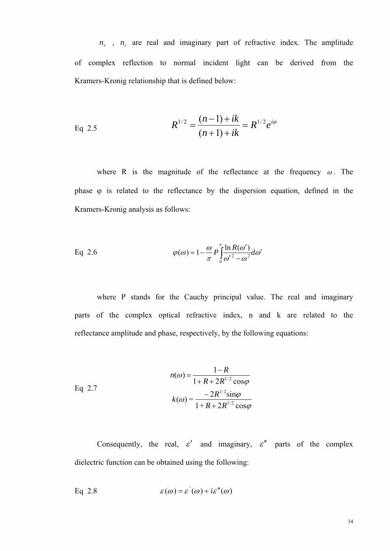
34

rn , in are real and imaginary part of refractive index. The amplitude

of complex reflection to normal incident light can be derived from the

Kramers-Kronig relationship that is defined below:

Eq 2.5 ϕieR

ikniknR 2/12/1

)1()1(

=+++−

=

where R is the magnitude of the reflectance at the frequency ω . The

phase ϕ is related to the reflectance by the dispersion equation, defined in the

Kramers-Kronig analysis as follows:

Eq 2.6 ωωωω

πωωϕ ′

−′′

−= ∫∞

dRP0

22

)(ln1)(

where P stands for the Cauchy principal value. The real and imaginary

parts of the complex optical refractive index, n and k are related to the

reflectance amplitude and phase, respectively, by the following equations:

Eq 2.7

ϕϕω

ϕω

cos2+1 sin2=)(

cos211)(

2/1

2/1

2/1

RRRk

RRRn

+−

++−

=

Consequently, the real, ε ′ and imaginary, ε ′′ parts of the complex

dielectric function can be obtained using the following:

Eq 2.8 )()( )( ' ωεωεωε ′′+= i

35

Eq 2.9 )()( 22 ωωε kn −=′

Eq 2.10 )()(2 ωωε kn=′′

The Kramers-Kronig relationship is a good mathematical tool for

extracting the real and imaginary parts of the refractive index (APPENDIX C).

2.4.2.3 Loss function

The imaginary part, also known as the extinction coefficient, is related

to the damping of the oscillation amplitude of the incident field. A non-metallic

material (dielectric) has low absorption, and the imaginary part is small and

often neglected. If the material is conductive, the imaginary part is larger and

must be taken into account. The energy-loss spectrum is closely related to a

quality referred to as the energy-loss function, Im [-1/()] (Imaginary part of -

1/()) via this relationship (Batson and Silcox, 1983; Ghasemifard, Zavar,

Ghasemifard et al., 2010).

Eq 2.11 222 ))()(()()(2)1Im(ωωωω

ε knkn

+=−

2.5 Magnetic field effect on materials

To understand the effects of magnetic fields on material, both quantum

and classic mechanics are required. Some phenomena can be described using

classical mechanics and some should be explained using quantum effects.

2.5.1 Classical mechanics

There are two types of forces that operate on electric charges and ions, q

that are placed inside magnetic and electric fields. Electric fields, E, apply a

force F=qE proportional to the intensity of the electric field and the magnitude

36

of the charge. This force is exerted regardless of the motion of the charge or

ion. Magnetic field, B, can only interact with moving ions and charged objects.

The magnetic force F=qv×B is restricted by the rule that only a charge, q,

moving in a non-parallel direction to B can experience a magnetic force. This

limitation is an important feature of the Lorentz force.

The equation of motion for a particle of charge q and mass m under the

Lorentz force is given by the following:

Eq 2.12

This equation requires the particle to accelerate and reach a velocity .

Here v is the particle's velocity and ^ denotes the cross product. The electric

field in a real system does not extend to infinity, implying that collisions do

slow down the particle. When E=0, B=B0Z, the charge accelerates and velocity

can be derived as shown below:

Eq 2.13

dvx

dt=

qm

vyB0

dvy

dt= −

qm

vx B0

dvz

dt= 0

The contraction induced by the Lorentz force power and the liquid environment

is largely based on dipole-dipole interactions and the free charge interactions that could

cause significant differences between their magnitudes. Another mechanism that is

important in the interaction between biological samples and a static magnetic field is

bound ion dynamics. The oscillation of a bound ion about its binding portion in a

signalling molecule can affect its ionic transport. These equations are easily solved as

mdvdt

= q E+ v∧ B( )

http://en.wikipedia.org/wiki/Cross_product

37

Eq 2.14. The x,y and z index indicate the direction of velocity and show perpendicular

direction. Wc is and f is .

Eq 2.14

vx = vx0e± iωc t

vy = vy0e±iω c t where ωc =

qm

B0

vz = vz 0

vx = v⊥ 0 cos ωct +ϕ( )vy = −v⊥ 0 sin ωct +ϕ( )vz = vz0

This magnetisation causes the cell to experience a rotational torque

caused by the static magnetic field. Effect of magnetic field on the orientation

of molecules and moving charged objects is the most important when exposed

to biomaterials, such as large organised structures (e.g., DNA and proteins).

The ionic side of DNA move faster and faster due to the Lorentz force,

according to Eq 2.16.

Eq 2.15 ( ) ( )

TKmVvvmK

mVdtd

byx

DM

==+=

=+=

222

21)(

21

,FFF

K indicates the kinetic energy, m and v are mass and velocity of ions,

respectively, and bK and T are the Boltzmann constant and the temperature,

respectively.

2.5.2 Quantum mechanics of the magnetic field effects on materials

An electron can spin around a nucleus and also has an intrinsic spin

around its own axis. Angular momentum follows the right hand rule. The

angular momentum and the magnetic moment are in the same direction (Figure

2.16) as that caused by the spin of the nucleus.

38

Figure 2.16 The angular momentum vector, L, can lie along specific

orientations with respect to the external magnetic field.

The magnetic momentum vector, m, can lie along specific orientations

with respect to the same direction or opposite direction of external magnetic

field (Figure 2.17).

Figure 2.17 An atom is placed in a magnetic field with the convention that the

South Pole is at the top and the North Pole is at the bottom.

B

N

N

N

N ml=+1

ml=0 ml=-1

highest energy lowest energy state state

S

39

2.5.2.1 The Zeeman Effect

When an atom with J > 0 is placed in a magnetic field, spectral lines

split into components. Therefore, by applying a magnetic field B, the energy

levels of an atom change by an amount –μ⋅B. Indeed, the energies of the

absorbed and emitted photons will change. This effect was observed for the

first time in 1896 by Zeeman before the development of quantum mechanics

and is called the Zeeman effect (Atkins and Friedman, 1997). The energy

difference between adjacent levels is described below:

Eq 2.16 JBMJ MBE ..μ=

Figure 2.18 The difference in energy between adjacent levels

As shown in Figure 2.18, when the splitting of the energy levels after

applying a magnetic field is the same for the lower and upper levels, only three

lines result from the 9 transitions. The splitting for S = 0 is the same and is

known as the normal Zeeman Effect. Energy equation for the normal Zeeman

Effect is as follows:

no field field

J = 2

J = 1

M J210

-1-2

40

Eq 2.17 BMEE BJMJ ..0 μ+=

The magnitude of the energy shift, ΔE, after applying a magnetic field is

given by Eq 2.17 and Eq 2.18 as follows:

Eq 2.18 EΔ =− ⋅Bμ

Eq 2.19 e

.2

em

⎛ ⎞= ⋅⎜ ⎟⎝ ⎠

L B

If the z axis is selected to be in the same direction as the magnetic field

B, then Eq 2.20 simplifies to:

Eq 2.20

in which the values of Lz are hm ,

Eq 2.21

and must have the same dimensions as the magnetic moment. This

quantity is called the Bohr magneton μB, in Atomic Physics with the value:

Eq 2.22 μ 5.79 10 /

Eq 2.23 μ ħ 9.27 10 .

Eq 2.22 can be rewritten in terms of μB as follows:

e

,2 z

eE L Bm

⎛ ⎞Δ = ⎜ ⎟

⎝ ⎠

e

.2eE mBm

⎛ ⎞Δ = ⎜ ⎟

⎝ ⎠

h

41

Eq 2.24 B .E m BμΔ =

where there are 2l + 1 states of m: 1, l – 1, . . . , – l.

2.5.2.2 The anomalous Zeeman Effect

Splitting for S > 0 is different for the upper and lower levels and is

known as the anomalous Zeeman Effect. The anomalous Zeeman Effect

requires a factor of Jg :

Eq 2.25 E E M g BMJ J J B= +0 . . .μ

Anomalous Zeeman splitting is complicated and depends on the orbital

and spin moments. The simple case is a S state and l = 0. In this situation, the

atom would not have a magnetic moment and would be unaffected by a

magnetic field. In fact, the electron has spin, and there is a magnetic moment.

Eq 2.26 .

Eq 2.27

When a magnetic field B is applied in the z direction, the energy

changes in the following manner when Sz has the following values:

Eq 2.28 12 ,zS = ± h

e

.zeE S B

mΔ = − ⋅ =Bμ

42

Eq 2.29

The separation should be twice that of the normal Zeeman Effect. Thus,

the separation of levels=2µB.

2.5.2.3 The Paschen-Back Effect

The Paschen-Back regime (PBR) was described by Hill in 1929 and

described as the splitting of molecular doublet levels.

Figure 2.19 The splitting of the sodium D line when the amplitude of the

magnetic fields increase from low to high shows this effect.

For sufficiently large magnetic fields, the orbital angular momentum L

and the spin angular momentum S couple to the magnetic field separately.

Figure 2.19 shows the splitting of the sodium D line at the amplitude of the

magnetic fields. In this condition, the levels are characterised by ML and MS

values rather than MJ (Minaichev, Myasishcheva, Obukhov et al., 1970).

Be2

eE B Bm

μΔ =± =±h

no B small B large B M M L S

MJ

P 2 3/2

P 2 1/2

3/21/2

-1/2-3/2

1/2-1/2

1 +1/2

0 +1/2

-1 +1/21 -1/2

0 -1/2

-1 -1/2

43

In an external magnetic field, the expected Hamiltonian can be

calculated using the equations below:

Eq 2.30 sBlBsocf VVVHH +++=

Eq.. 2.31

( )( )

( ) ( )0

221

2 2

=⋅

⋅−⋅−⋅+=

LS

BSc

qgBLc

qgLSdr

rdVrc

gHH slscf

rr

rrrrrr

μμμ

Eq 2.32 ( ) ( ) BSc

eBLc

eHH cf

rrrr⋅+⋅+=

μμ2

In a strong magnetic field B, 0=⋅LSrr

, which is known as the Paschen-

Back Effect.

2.5.2.4 Raman spectroscopy

Raman spectroscopy is a spectroscopic method based on the scattering

of monochromatic light by a molecule. The usefulness of Raman scattering for

studying molecular vibrations was discovered in 1928 by C.V. Raman (Lin-

Vien, 1991).

The mechanisms by which electromagnetic radiation interacts with

molecular systems differ. Electromagnetic waves can interact with a vibrating

molecule if the electric field vector of the electromagnetic wave oscillates

along the dipole moment μ of the molecule. If the dipole moment of the

molecule and the normal vibration change, the molecule has an infrared-active

vibration.

44

Figure 2.20 Raman scattering mechanism, including Stokes, anti-Stokes and

Rayleigh scattering.

Raman spectroscopy is based on scattering. Electromagnetic radiation is

scattered by crystal or molecule. As a result of scattering, one photon from the

incident light is annihilated and one photon in the scattered radiation is created.

The scattering light can be classified by the difference between the

frequency of the incident and scattered light. In Rayleigh scattering, the

frequency of the incident light is equal to that of the scattered light. In Raman

scattering, the energy of the incident light is not equal to that of the scattered

light. The change in frequency leads to the Stokes and anti-Stokes scattering

effects. Figure 2.20 shows a schematic of Raleigh, Stokes and anti-Stokes

scattering. As shown in this figure, for Rayleigh scattering, the incident light

and the scattered light have the same energy. For Stokes and anti-Stokes

scattering, the scattered energy is smaller and larger, respectively, than the

incident energy. All electromagnetic waves have an electric field. The electric

field interacts with the charge distribution of a molecule (dipole moment) and

the resultant perturbation is proportional to the strength of the electric field.

45

Perturbed electron moves to another state, an exited state. Dipole moment

changes in the molecule according to Eq 2.33. α, E, μ and μ0 are the

polarizability, the electric field, the dipole momentum and the dipole

momentum in zero fields, respectively.

Eq 2.33 0 Eμ = μ + α

The excited electron returns to the initial state in Rayleigh scattering

and can move to a higher-energy state in Stokes scattering or a lower-energy

state in anti-Stokes scattering. All of these transitions should follow selection

rules (APPENDIX D).

Vibration modes in Raman spectroscopy obey the selection rule that

1Δν = ± for a harmonic oscillator and 1, 2, 3, 4, 5,Δν=± ± ± ± ± K for an

anharmonic oscillator. Not all vibrations can participate in Raman scattering.

Vibrations that change the molecule polarisability during the interaction will

have a Raman response.

46

3.1 CHAPTER III: DESIGN, METHODS AND PROCEDURE

3.1 Introduction

This chapter deals with the experimental part of the thesis, including the

materials, chip fabrication, set up and measuring instruments. The best

methods for extraction, measurements, fabrication and analysis were selected

using the following criteria; the available facility, the best accuracy, high

quality and safety. Each part of this chapter includes a brief explanation on the

possible regular methods for comparison with the presented method. Due to the

highly sensitive DNA samples and the microchip fabrication process, the

extraction and fabrication techniques were conducted in a controlled condition

of a 10K clean room.

3.2 Materials

A p-type Si wafer (orientation <100>) with a resistivity of 1 to 10–20

Ω-cm (MEMC Electronic Materials) was used as the substrate. The gold wire

(Kurt J. Lesker Company) that was used in the evaporation and magnetron

sputtering technique had a purity of 99.999%. Other necessary chemicals

(C2H5OH, deinonized water and acetone) and MicroChem’s SU-8 photoresist

and developer were supplied by Sigma Aldrich and were used without further

purification. Borosilicate or Pyrex glass was used as a substrate material with

an electrical resistivity of approximately 1013 Ω.m (William Jr, 2007). DNA

from Mimosa pudica (the sensitive plant) was extracted using the extraction kit

Gene All kit (Plant SV mini). The sample preparation in this work was divided

into two sections consisting of DNA extraction and oligonucleotide

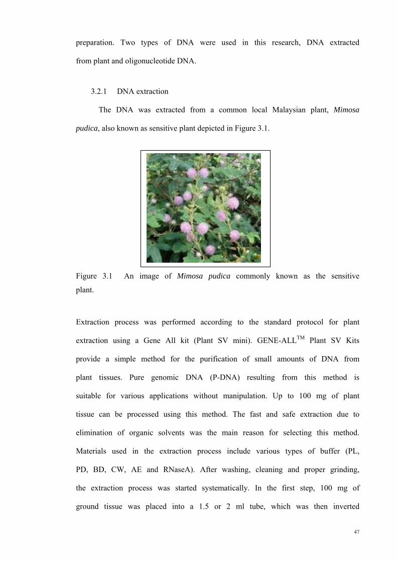
47

preparation. Two types of DNA were used in this research, DNA extracted

from plant and oligonucleotide DNA.

3.2.1 DNA extraction

The DNA was extracted from a common local Malaysian plant, Mimosa

pudica, also known as sensitive plant depicted in Figure 3.1.

Figure 3.1 An image of Mimosa pudica commonly known as the sensitive

plant.

Extraction process was performed according to the standard protocol for plant

extraction using a Gene All kit (Plant SV mini). GENE-ALLTM Plant SV Kits

provide a simple method for the purification of small amounts of DNA from

plant tissues. Pure genomic DNA (P-DNA) resulting from this method is

suitable for various applications without manipulation. Up to 100 mg of plant

tissue can be processed using this method. The fast and safe extraction due to

elimination of organic solvents was the main reason for selecting this method.

Materials used in the extraction process include various types of buffer (PL,

PD, BD, CW, AE and RNaseA). After washing, cleaning and proper grinding,

the extraction process was started systematically. In the first step, 100 mg of

ground tissue was placed into a 1.5 or 2 ml tube, which was then inverted

48

(lysis) several times. Next, 400 µl of buffer PL and 4 µl of RNase were added

to the solution and vortexed, followed by incubation for 10 to 15 min at 65°C.

The solution was then filtered, centrifuged and transferred by pass-through to a

new tube. In the next step, 1.5 ml of buffer BD was added and mixed

immediately for optimal binding. In washing and elution steps, 700 µl of

mixture was placed in a filter tube, followed by centrifugation (30 seconds).

The supernatant was then discarded through the pass-through. Next, 300 µl of

buffer CW was added and centrifuged for 2 min. In the last step, 100 µl of

buffer AE was added and incubated for 5 min at room temperature, followed

by centrifugation for an additional 1 min ( The protocol shown in Figure 3.2

step by step).

Figure 3.2 DNA extraction protocol

Grind fresh or frozen plant tissue

Add Buffer 1 and Vortex and incubate for 10 ~ 15 min at 65˚C.

Add 140 ul of Buffer 2 and vortex for 5 min on ice

Apply to Filter and centrifuge and add Buffer 3 and mix

Apply to the filter tube and Centrifuge

Apply Buffer 4 to the Column, centrifuge.

Add 300 ul of Buffer 5 to the Column and Centrifuge

Add Buffer 6 and Incubate at room temperature and centrifuge

49

3.2.2 Oligonucleotide

Oligonucleotides are short lengths of nucleic acid polymers, typically

with 200 or fewer bases. Two types of oligonucleotide DNA were used in this

research; either adenine (A) - thymine (T) pairs or cytosine (C) - guanine (G)

pairs. The properties of the used oligos such as molecular weight and melting

temperature are respectively 30817.6 and 59.48 for 100 mer AT and for 100

mer CG are 30777.5 and 101.25.

Table 3-1 Oligonucleotide DNA feature used in this work

Oligonucleotide Molecular Weight Melting temperature Number (mer)

AT-100 30817.6 59.48 100

CG-100 30777.5 101.25 100

3.3 Fabrication of chip

The fabrication consists of several basic steps. A brief overview of the

fabrication process, including the cleaning, mask design, lithography and

deposition is presented.

3.3.1 Cleaning

There are regular processes involving liquid solvents to clean common

samples and substrates, such as silicon, glass and wafers (Banks, 2006). The

materials and equipment for these processes are available in a clean room

environment as part of the common facilities. After cutting the silicon or

substrate manually or using a regular cutter, the cleaning process should be

performed using standard RCA method. Simple cleaning process for removing

contamination: 1. Rinse the wafer in acetone , 2. Scrub the wafer properly

using a swab, 3. Wash the wafer with DI water, 4. Dry the wafer using nitrogen

gas

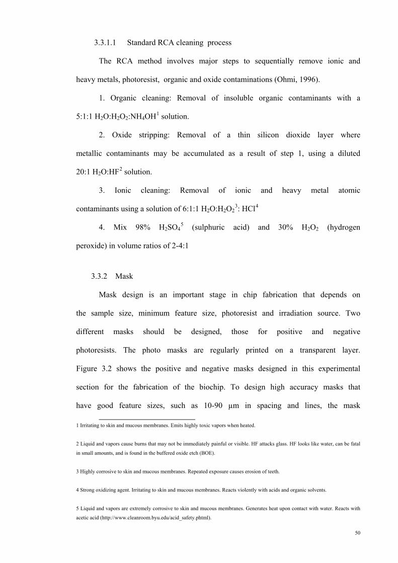
http://eu.idtdna.com/analyzer/applications/Instructions/Default.aspx?AnalyzerDefinitions=true#MolecularWeight

50

3.3.1.1 Standard RCA cleaning process

The RCA method involves major steps to sequentially remove ionic and

heavy metals, photoresist, organic and oxide contaminations (Ohmi, 1996).

1. Organic cleaning: Removal of insoluble organic contaminants with a

5:1:1 H2O:H2O2:NH4OH1 solution.

2. Oxide stripping: Removal of a thin silicon dioxide layer where

metallic contaminants may be accumulated as a result of step 1, using a diluted

20:1 H2O:HF2 solution.

3. Ionic cleaning: Removal of ionic and heavy metal atomic

contaminants using a solution of 6:1:1 H2O:H2O23: HCl4

4. Mix 98% H2SO45 (sulphuric acid) and 30% H2O2 (hydrogen

peroxide) in volume ratios of 2-4:1

3.3.2 Mask

Mask design is an important stage in chip fabrication that depends on

the sample size, minimum feature size, photoresist and irradiation source. Two

different masks should be designed, those for positive and negative

photoresists. The photo masks are regularly printed on a transparent layer.

Figure 3.2 shows the positive and negative masks designed in this experimental

section for the fabrication of the biochip. To design high accuracy masks that

have good feature sizes, such as 10-90 µm in spacing and lines, the mask

1 Irritating to skin and mucous membranes. Emits highly toxic vapors when heated.

2 Liquid and vapors cause burns that may not be immediately painful or visible. HF attacks glass. HF looks like water, can be fatal

in small amounts, and is found in the buffered oxide etch (BOE).

3 Highly corrosive to skin and mucous membranes. Repeated exposure causes erosion of teeth.

4 Strong oxidizing agent. Irritating to skin and mucous membranes. Reacts violently with acids and organic solvents.

5 Liquid and vapors are extremely corrosive to skin and mucous membranes. Generates heat upon contact with water. Reacts with

acetic acid (http://www.cleanroom.byu.edu/acid_safety.phtml).

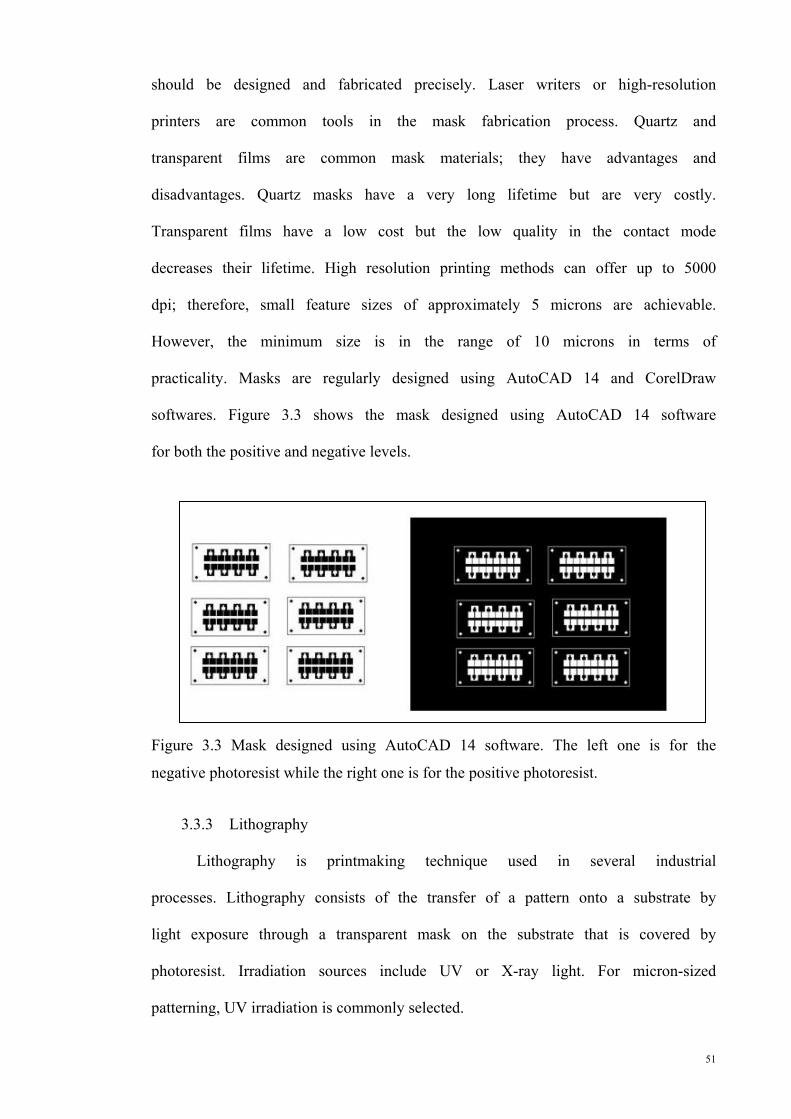
51

should be designed and fabricated precisely. Laser writers or high-resolution

printers are common tools in the mask fabrication process. Quartz and

transparent films are common mask materials; they have advantages and

disadvantages. Quartz masks have a very long lifetime but are very costly.

Transparent films have a low cost but the low quality in the contact mode

decreases their lifetime. High resolution printing methods can offer up to 5000

dpi; therefore, small feature sizes of approximately 5 microns are achievable.

However, the minimum size is in the range of 10 microns in terms of

practicality. Masks are regularly designed using AutoCAD 14 and CorelDraw

softwares. Figure 3.3 shows the mask designed using AutoCAD 14 software

for both the positive and negative levels.

Figure 3.3 Mask designed using AutoCAD 14 software. The left one is for the

negative photoresist while the right one is for the positive photoresist.

3.3.3 Lithography

Lithography is printmaking technique used in several industrial

processes. Lithography consists of the transfer of a pattern onto a substrate by

light exposure through a transparent mask on the substrate that is covered by

photoresist. Irradiation sources include UV or X-ray light. For micron-sized

patterning, UV irradiation is commonly selected.

52

3.3.3.1 Photo resist

A photoresist is a material that responds to the specific light used in the

lithography process. Two types of photoresist are offered; negative and

positive. For positive photoresists, the portions that absorb the light irradiation

are removed after completing the process and vice versa. The unexposed

portions will be polymerised and are difficult to dissolve, thus remaining on

the surface and appearing as negative photoresist. Figure 3.4 schematically

shows the patterns fabricated using positive and negative photoresists. Coating,

baking, exposure, developing and all other processes should be performed in

clean room conditions with yellow ambient light to obtain high quality

patterns. Table 3-2 shows categorises of several popular photoresist (negative

and positive) materials used in lithography (Banks, 2006).

Figure 3.4 Patterns fabricated using positive and negative photoresists, positive

(left) and negative (right)

53

AZ, Shipley, Nlof and SU-8 series are some common photoresists

utilised in micro- and nanoengineering. In the present work, SU-8-3000 was

selected due to its high sensitivity to the concentration of developer and the

high aspect ratio (> 10:1) compared with that of other photoresists.

A p-type Si wafer (orientation <100>) possessing a resistivity of 1 to

10–20 Ω-cm (MEMC Electronic Materials) was used as the substrate.

MicroChem’s SU8 photoresist and developer were supplied by Sigma Aldrich.

SU-8 3000 is an epoxy-based photoresist used for micromachining and

microelectronic purposes that provides high contrast and thermally stable

images. The standard SU-8 patterning processes is as follows; spin coat, soft

bake, expose, PEB and develop. Figure 3.5 shows the sequence of the

lithography process. Figure 3.6 depicts the procedure used to create a layer of

SU-8 photoresist on prepared substrate.

Table 3-2 Categorisation of popular photoresists used in micro-engineering

(Banks, 2006).

Positive Photo resist Developer Type

AZ 3312 AZ300MIF Positive

AZ 3330 AZ300MIF Positive

Shipley 1.2 L Shipley MF-26A Positive

Shipley 1.8 M Shipley MF-26A Positive

Nlof 2020 110°C/60s Negative

SU-8-2000.5 SU-8 Developer, gently agitate Negative

SU-su8-3000 SU-8 Developer, gently agitate Negative

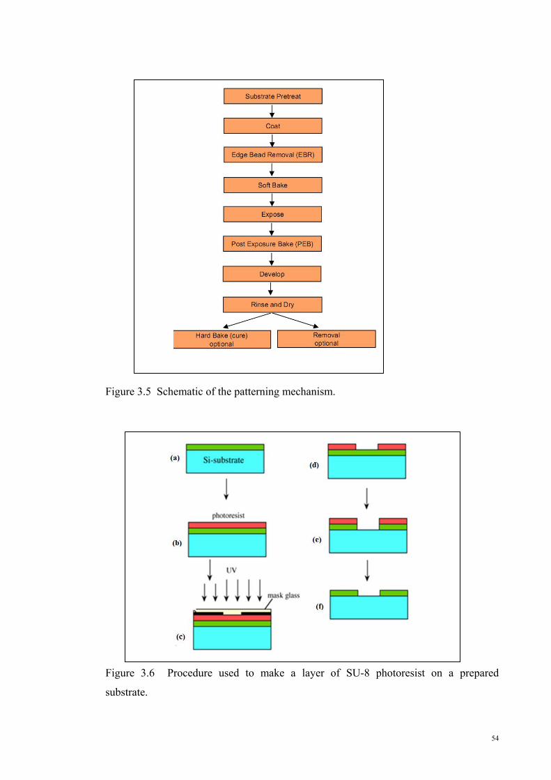
54

Figure 3.5 Schematic of the patterning mechanism.

Figure 3.6 Procedure used to make a layer of SU-8 photoresist on a prepared

substrate.

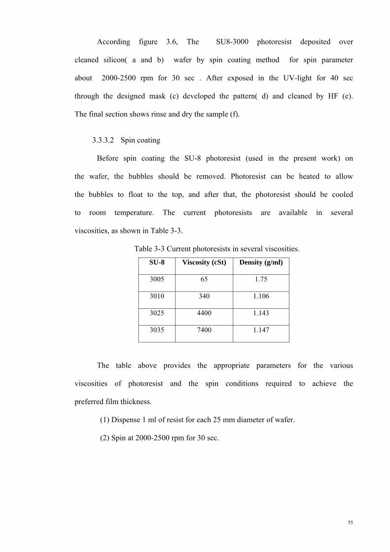
55

According figure 3.6, The SU8-3000 photoresist deposited over

cleaned silicon( a and b) wafer by spin coating method for spin parameter

about 2000-2500 rpm for 30 sec . After exposed in the UV-light for 40 sec

through the designed mask (c) developed the pattern( d) and cleaned by HF (e).

The final section shows rinse and dry the sample (f).

3.3.3.2 Spin coating

Before spin coating the SU-8 photoresist (used in the present work) on

the wafer, the bubbles should be removed. Photoresist can be heated to allow

the bubbles to float to the top, and after that, the photoresist should be cooled

to room temperature. The current photoresists are available in several

viscosities, as shown in Table 3-3.

Table 3-3 Current photoresists in several viscosities.

SU-8 Viscosity (cSt) Density (g/ml)

3005 65 1.75

3010 340 1.106

3025 4400 1.143

3035 7400 1.147

The table above provides the appropriate parameters for the various

viscosities of photoresist and the spin conditions required to achieve the

preferred film thickness.

(1) Dispense 1 ml of resist for each 25 mm diameter of wafer.

(2) Spin at 2000-2500 rpm for 30 sec.

56

3.3.3.3 Soft bake

In the soft bake stage, the samples should be heated up in uniform

thermal conditions to achieve a good aspect ratio and reduce the solvent level.

The recommended time and temperature for soft baking is shown in Table 3.4.

Table 3-4 Soft bake times for different thicknesses of SU-8 photoresist.

Thickness (microns) Soft Bake Time (minutes) at 90°c)

4-10 2-3

8-15 5-10

20-50 10-15

30-80 10-30

40-100 15-45

3.3.3.4 Exposure

Table 3-5 Exposure dose for different thicknesses of SU-8 photoresist.

Thickness (microns) Exposure Energy MJ/cm2

4-10 100-200

8-15 125-200

20-50 150-250

30-80 150-250

40-100 150-250

57

Table 3-6 Exposure dose for different substrates for SU-8 photoresist.

Material Relative Dose (x/times)

Silicon 1x

Glass 1.5x

Pyrex 1.5x

Indium Tin Oxide 1.5x

Silicon Nitride 1.5-2x

Gold 1.5-2x

Aluminum 1.5-2x

Nickel Iron 1.5-2x

Copper 1.5-2x

Nickel 1.5-2x

Titanium 1.5-2x

The exposure time and dose depend on the thickness of the photoresist.

Recommended exposure times and doses are shown in Tables 3-5 and 3-6.

3.3.3.5 Post exposure bake (PEB)

The post-exposure bake should occur directly after exposure at a

temperature between 90-95°C for 60 minutes although ramping up the

temperature and starting at a lower temperature near 50°C shows better result.

Furthermore, slowly ramping the temperature down is recommended after PEB

to prevent cracks and stress problems. Table 3-7 indicates the post-exposure

bake times for different thickness of SU-8 photoresist. The best parameter for

SU-8 that used in this work is 95 C and 1 min (after several test to optimize the

pattern).

58

Table 3-7 Post-exposure bake times for different thickness of SU-8 photoresist.

Thickness

(microns)

PEB Time (minute)

at 65°c

PEB Time (minutes)

at 95°c

4-10 1 1-2

8-15 1 2-4

20-50 1 3-5

30-80 1 3-5

40-100 1 3-5

3.3.3.6 Development

The developer for the SU-8 photoresist is based on acetone, which

removes material. The largest issue is that when drying the acetone, some

thermal-expansion occurs at the film. Recommended times for developing

immersion the processes are shown in Table 3-8.

Table 3-8 Development times for different thicknesses of the SU-8 developer

Thickness (microns) Development Time (minutes)

4-10 1-3

8-15 4-6

20-50 5-8

30-80 6-12

40-100 7-15

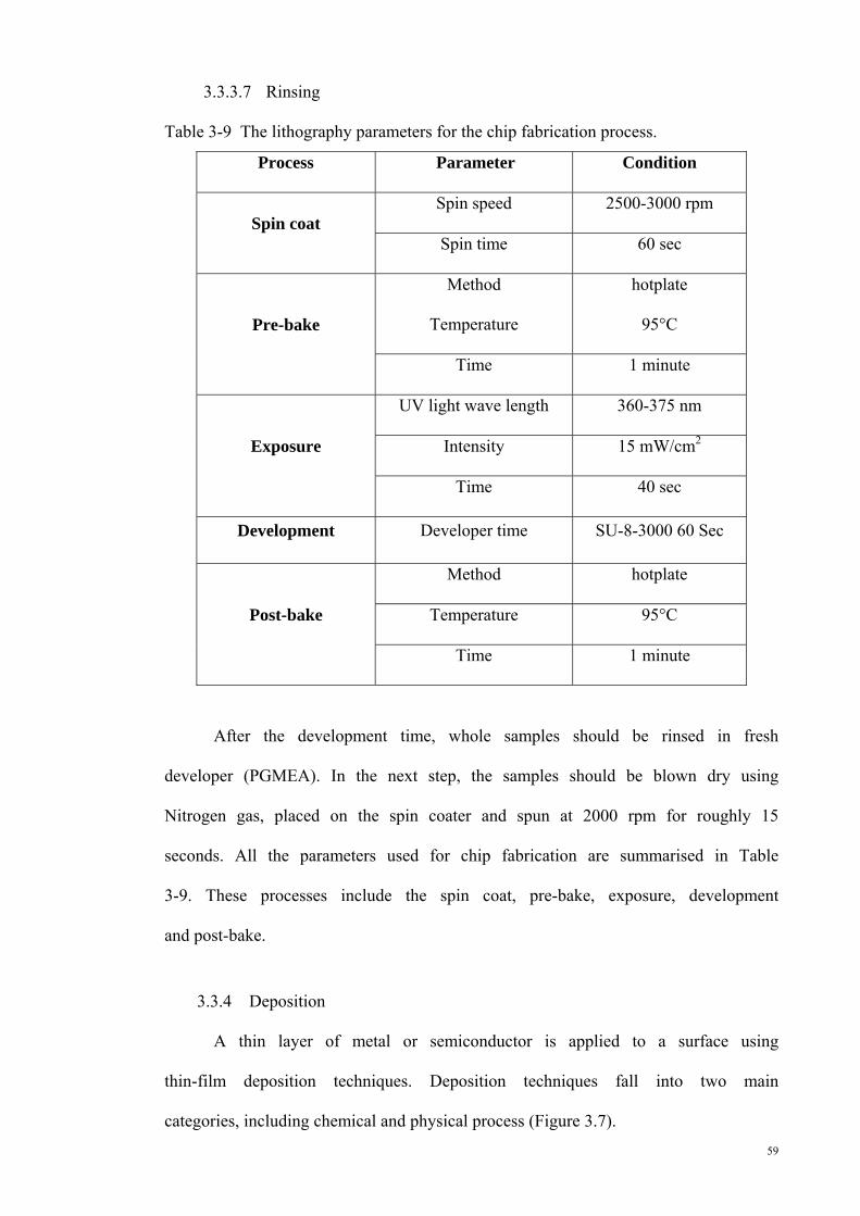
59

3.3.3.7 Rinsing

Table 3-9 The lithography parameters for the chip fabrication process.

Process Parameter Condition

Spin coat Spin speed 2500-3000 rpm

Spin time 60 sec

Pre-bake

Method

Temperature

hotplate

95°C

Time 1 minute

Exposure

UV light wave length 360-375 nm

Intensity 15 mW/cm2

Time 40 sec

Development Developer time SU-8-3000 60 Sec

Post-bake

Method hotplate

Temperature 95°C

Time 1 minute

After the development time, whole samples should be rinsed in fresh

developer (PGMEA). In the next step, the samples should be blown dry using

Nitrogen gas, placed on the spin coater and spun at 2000 rpm for roughly 15

seconds. All the parameters used for chip fabrication are summarised in Table

3-9. These processes include the spin coat, pre-bake, exposure, development

and post-bake.

3.3.4 Deposition

A thin layer of metal or semiconductor is applied to a surface using

thin-film deposition techniques. Deposition techniques fall into two main

categories, including chemical and physical process (Figure 3.7).

http://en.wikipedia.org/wiki/Chemistry

http://en.wikipedia.org/wiki/Physics

60

3.3.4.1 Chemical deposition

For chemical deposition, a chemical change occurs at a solid surface

and results in a solid layer. This process includes plating, chemical solution

deposition (CSD) or chemical bath deposition (CBD), spin coating, chemical

vapour deposition (CVD) and atomic layer deposition (ALD).

3.3.4.2 Physical deposition

Physical deposition uses mechanical and electromechanical methods to

create a thin layer of a solid film on a substrate. Physical deposition techniques

include electron beam evaporation, molecular beam epitaxial (MBE),

sputtering, pulsed laser deposition, cathode arc deposition (arc-PVD) and

electro hydrodynamic deposition (Figure 3.7).

Figure 3.7 Deposition techniques; chemical and physical processes.

The two methods used to fabricate thin metal layers in the present work

are described. These processes are often utilised in the semiconductor industry

to make thin films of Al and gold. Thermal evaporators are chosen for thicker

layers of metal and have poorer control over the rate of the deposition.

http://en.wikipedia.org/wiki/Sol-gel

http://en.wikipedia.org/wiki/Sol-gel

http://en.wikipedia.org/wiki/Chemical_bath_deposition

http://en.wikipedia.org/wiki/Spin_coating

http://en.wikipedia.org/wiki/Chemical_vapor_deposition

http://en.wikipedia.org/wiki/Chemical_vapor_deposition

http://en.wikipedia.org/wiki/Atomic_layer_deposition

http://en.wikipedia.org/wiki/Electron_beam_physical_vapor_deposition

http://en.wikipedia.org/wiki/Molecular_beam_epitaxy

http://en.wikipedia.org/wiki/Sputtering

http://en.wikipedia.org/wiki/Pulsed_laser_deposition

http://en.wikipedia.org/wiki/Cathodic_arc_deposition

http://en.wikipedia.org/wiki/Electrohydrodynamic

http://en.wikipedia.org/wiki/Chemistry

http://en.wikipedia.org/wiki/Physics

http://en.wikipedia.org/wiki/Semiconductor_industry

http://en.wikipedia.org/wiki/Thin_film

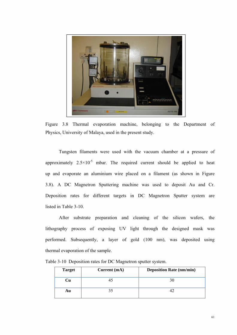
61

Figure 3.8 Thermal evaporation machine, belonging to the Department of

Physics, University of Malaya, used in the present study.

Tungsten filaments were used with the vacuum chamber at a pressure of

approximately 2.5×10-5 mbar. The required current should be applied to heat

up and evaporate an aluminium wire placed on a filament (as shown in Figure

3.8). A DC Magnetron Sputtering machine was used to deposit Au and Cr.

Deposition rates for different targets in DC Magnetron Sputter system are

listed in Table 3-10.

After substrate preparation and cleaning of the silicon wafers, the

lithography process of exposing UV light through the designed mask was

performed. Subsequently, a layer of gold (100 nm), was deposited using

thermal evaporation of the sample.

Table 3-10 Deposition rates for DC Magnetron sputter system.

Target Current (mA) Deposition Rate (nm/min)

Cu 45 30

Au 35 42

62

3.4 Set up preparation

As depicted in Figure 3.9, a Helmholtz coil pair system with a

cylindrical cap (with a 2500 W DC power supply, 4500D Electromagnet 3472-

50)6 was used to create the magnetic field. Helmholtz coils can provide a very

homogeneous magnetic field using a cylindrical cap.

Figure 3.9 A side view of the magnetic field generator used in this work. Two coils are located parallel to each other and separated by a small distance.

Two coils are located parallel to each other and separated by a small

distance comparable to the diameter of the microtube that creates a

homogeneous magnetic field in the centre between the coils. A side view of

magnetic field generator (Helmholtz coil) is shown in Figure 3.10. As shown

as figure 3.9, there are two handle to adjust the poles to the desired gap (a), two

6 Personnel Safety: During operation, the magnet fringing field is greater than 0.5 mT (5 G). This field can cause heart pacemakers and

other medical implants to malfunction. We recommend that the fringing field should be mapped, and warning signs should be placed outside the 0.5

mT (5 G) contour. Entry to this region should be restricted to qualified personnel.

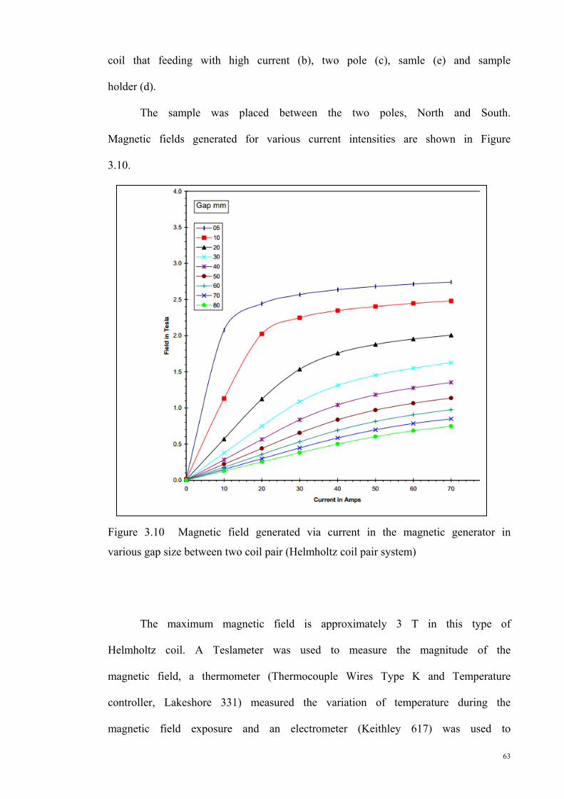
63

coil that feeding with high current (b), two pole (c), samle (e) and sample

holder (d).

The sample was placed between the two poles, North and South.

Magnetic fields generated for various current intensities are shown in Figure

3.10.

Figure 3.10 Magnetic field generated via current in the magnetic generator in

various gap size between two coil pair (Helmholtz coil pair system)

The maximum magnetic field is approximately 3 T in this type of

Helmholtz coil. A Teslameter was used to measure the magnitude of the

magnetic field, a thermometer (Thermocouple Wires Type K and Temperature

controller, Lakeshore 331) measured the variation of temperature during the

magnetic field exposure and an electrometer (Keithley 617) was used to

64

investigate the magnetic field effects on the resistivity before and after the

exposure of a DNA solution to the magnetic field. A digital timer was used to

control the measurement and exposure times.

3.5 Analysis and measuring

DNA strands (5 to 20 µl) were diluted and exposed to the magnetic

field. Figure 3.11 shows a schematic of the set up elements, instruments and

wire connections , and Figure 3.12 displays the overall set up used in this

work. The cell containing the DNA is located in the centre of the coil, where

the magnetic field is uniform (25°C and 2 to 10 min). UV-Vis spectrum was

measured using a Perkin Elmer 750UV-Vis spectrometer. A DI is used as

background sample. DI water have no peak in the region 200-350 nm, was

utilized to dilution DNA. The micro-Raman spectroscopic analysis was

performed after preparing a sample of p-type silicon that was cleaned and

coated with 80 nm of gold via the thermal evaporation technique. A Ranishaw

inVia micro-Raman spectrometer at 514 nm was used to record the spectra.

Experiments were repeated after several extractions to eliminate low

concentration of samples after extraction; the UV-Vis measurement carried out

three times for each sample. The results were analysed using softwares

(Microsoft Excel, SPSS and Spectrum Analyzer) statistically.

65

Figure 3.11 Measurement set up, including AVO meter, Tesla meter, timer, thermometer , magnetic generator that included power supply and electromagnet and wire connections .

Figure 3.12 Diluted DNA sample placed in the magnetic field region (a)

Electromagnet; (b) Thermometer; (c) Multimeter; (d) Timer; (e) Teslameter; (f)

Electromagnet power supply and (g) DNA sample.

66

As depicted in Figure 3.10 thermal controlling device and thermometer

used for decrease and increase and monitoring temperature, tesla meter used to

measure the strength of magnetic field, AVO measurement units utilized for

measuring current via voltage and resistivity and electromagnet, electromagnet

power supply and Programmable power supply used to generate and tune

magnetic field.

67

4.1 CHAPTER IV:RESULTS AND DISCUSSIONS: BIOLOGICAL

PERSPECTIVE

4.1 Introduction

The first part of research findings is presented in this chapter. Analysis

carried-out is categorized into two perspectives covering the biological and

Physics aspects as shown in the flow chart in Figure 4.1. Two types of DNA

samples were analysed namely native DNA extracted from plant and

oligonucleotide DNA. Measurements were done before and after exposure to

magnetic fields of different strengths. The magnetic field was tuned to the

required magnitude prior to each measurement.

Figure 4.1 Flow-chart showing the two perspectives of analyses done in this

work based on the biological and Physics aspects.

UV-Vis and Raman spectroscopy measurements were done on the DNA

samples to study the effects of magnetic field exposure on parameters derived

Analysis parameters

Physics Aspect

Temperature Analysis

Spectroscopy Analysis

UV‐VIS Spectroscopy

Loss Function Refractive Index

Band Gap

Raman Spectroscopy

Resistivity Analysis

Biological Aspect

UV‐VIS Spectrum

Extinction Coefficient Purity Concentration

68

from these measurements. The band gap, refractive index, loss functions and

bond vibrations were the parameters analysed from the Physics perspective.

Purity and extinction coefficient meanwhile were the parameters investigated

from the biological perspective. Resistance and temperature measurements

were done in magnetic fields of different strengths to study the influence of the

field on these parameters. The results were presented in the next chapter along

with the parameters derived from the UV-Vis and Raman results analysed from

the Physics perspective. All the fundamental goals defined in the objectives

listed in Chapter 1 drove towards the collection of data and the subsequent data

analysis.

In μ-Raman spectroscopy, the spot size of the scanning laser beam is

only a few micrometers in diameter. For DNA deposited on the ultra-thin film

of gold, this size provides accurate spatial information on the characteristics of

the sample such as the chemical composition of the sample.

UV-Vis spectroscopy is used to investigate the absorbance spectra of

DNA molecules in solution. UV-Vis data can provide qualitative as well as

quantitative analysis and information. DNA bases absorb light at wavelength of

260 nm, and this value is used to determine DNA properties. Absorption

spectroscopy is commonly used on organic materials to investigate the

aromatic conjugation within molecules. Usually, organic materials are used in

the form of liquid solutions for this measurement. Solvents, such as water and

ethanol do not absorb in the UV-Vis spectral region and therefore can be used

as the solvent for organic compounds and this includes DNA. The logarithmic

ratio between the incident radiation and the radiation transmitted through

diluted DNA is measured and can be used in the Beer-Lambert law to

determine the optical density, a dimensionless parameter. According to the

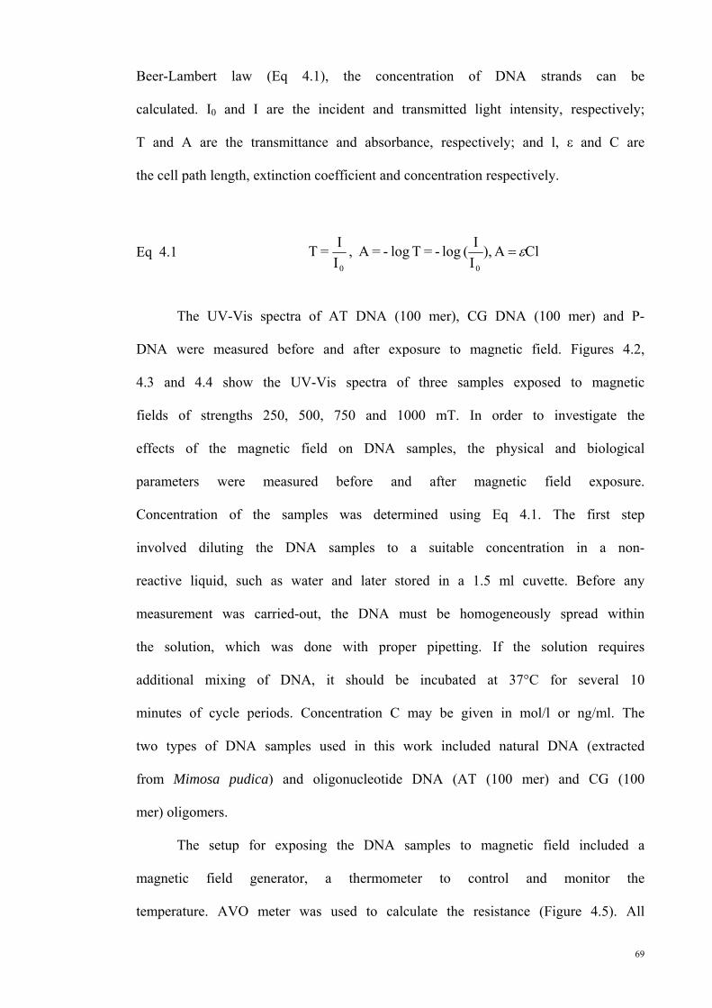
69

Beer-Lambert law (Eq 4.1), the concentration of DNA strands can be

calculated. I0 and I are the incident and transmitted light intensity, respectively;

T and A are the transmittance and absorbance, respectively; and l, ε and C are

the cell path length, extinction coefficient and concentration respectively.

Eq 4.1 ClA ),II( log - = T log- =A ,

II= T

00

ε=

The UV-Vis spectra of AT DNA (100 mer), CG DNA (100 mer) and P-

DNA were measured before and after exposure to magnetic field. Figures 4.2,

4.3 and 4.4 show the UV-Vis spectra of three samples exposed to magnetic

fields of strengths 250, 500, 750 and 1000 mT. In order to investigate the

effects of the magnetic field on DNA samples, the physical and biological

parameters were measured before and after magnetic field exposure.

Concentration of the samples was determined using Eq 4.1. The first step

involved diluting the DNA samples to a suitable concentration in a non-

reactive liquid, such as water and later stored in a 1.5 ml cuvette. Before any

measurement was carried-out, the DNA must be homogeneously spread within

the solution, which was done with proper pipetting. If the solution requires

additional mixing of DNA, it should be incubated at 37°C for several 10

minutes of cycle periods. Concentration C may be given in mol/l or ng/ml. The

two types of DNA samples used in this work included natural DNA (extracted

from Mimosa pudica) and oligonucleotide DNA (AT (100 mer) and CG (100

mer) oligomers.

The setup for exposing the DNA samples to magnetic field included a

magnetic field generator, a thermometer to control and monitor the

temperature. AVO meter was used to calculate the resistance (Figure 4.5). All

70

samples were placed at the centre of a uniform magnetic field for 10 minutes.

After the spectrophotometer was turned on, the absorbance and transmittance

of the samples were measured.

Figure 4.2 UV-Vis spectra of diluted AT-100 DNA sample after exposure to

magnetic fields of various strengths (250, 500, 750 and 1000 mT).

Figure 4.3 UV-Vis spectrum of diluted CG-100 DNA sample after exposure to

magnetic fields of various strengths (250, 500, 750 and 1000 mT).

71

Figure 4.4 UV-Vis spectrum of diluted P-DNA sample after exposure to

magnetic fields of various strengths (250, 500, 750 and 1000 mT)

Figure 4.5 The measurement setup included a magnetic field generator for

applying a uniform magnetic field, a thermometer to control and monitor the

temperature and an AVO meter to calculate the resistance. A drop of diluted

DNA placed between two metal electrode.

72

All measurements were performed before and after magnetic field

exposure by tuning the strength of the magnetic field. The biological analysis

included analysis of the purity, optical density, maximum wavelength and

extinction coefficient.

4.2 Purity calculation

Proteins, which can contaminate extracted DNA, can absorb light in the

ultraviolet region. The ratio of absorbance at 260 and 280 nm can be used to

assess the purity of DNA samples since DNA and proteins absorb light most

strongly at 260 nm and 280 nm respectively. This ratio is used to investigate

the purity of DNA before and after exposure to a magnetic field. If the ratio of

the absorbance of DNA sample at 260 nm is above 1.75, the DNA should be

pure enough to proceed for further measurements. The variation in the purity of

the measured diluted p-DNA samples with the magnitude of the magnetic field

strength exposure is shown in Figure 4.6.

Figure 4.6 The variation in the purity of diluted DNA samples (P-DNA, AT-

100 and CG-100) against the magnitude of magnetic field strengths.

73

As depicted in Figure 4.6, the purity of DNA samples ( ratio of Optical

density in 260 to 280) exposed to magnetic field did not decrease. The ratio of

the absorbance at 260 nm to that at 280 nm did not change significantly. In

spite of the change in the optical density after exposure to the magnetic field,

as shown in Figures 4.3, 4.4 and 4.5, the purity remained constant for AT-100

and P-DNA and slightly increased for CG-100. This result occurred because of

the decreased amount of contamination in the CG-100 solution. Indeed, the

contamination in CG-100 was already greater than that in the other two

samples because of the synthesis process (Because of low potential energy of

the G base make synthesis difficult). The magnetic field did not decrease the

amount of contamination; however, the contaminants were deposited in the

solution because of the Lorentz force. Due to the difference in the magnetic

response of the DNA and the contamination in the water, the contamination in

the water drifted in a specific direction and precipitated (Iwasaka and Ueno,

1998). The magnetic field acted as a filter to separate the contaminant because

of its different susceptibility and weight.

Table 4-1 The statistical regression analysis for the purity curve of AT-100,

CG-100 and P-DNA exposed to the magnetic field.

Purity Coefficients p-Value

AT

Intercept 1.99±0.02 2.16×10-6

X Variable 1 -1.12×10-5 0.57

CG

Intercept 1.69±0.03 2.11×10-6

X Variable 1 2.03×10-4 0.40

P-DNA

Intercept 1.81±0.01 1.16×10-6

X Variable 1 -3.60×10-5 0.23

74

Table 4-1 shows the statistical regression analysis from the purity curve

measured with a magnetic field, which is also shown in Figure 4.6. According

to the p-value shown in Table 4-1, there is a meaningful relationship between

the purity and the magnetic field strength based on the p-value. The intercept

and X p-values for AT-100, CG-100 and P-DNA are 0.57; 2.16×10-6, 0.40;

2.11×10-6 and 0.23; 1.16×10-6, respectively, and their standard errors are 0.02,

0.03 and 0.01, respectively.

4.3 Extinction coefficient

Extinction coefficient can be used to evaluate the absorption of light in

a material. In Biochemistry and Molecular Biology, the molar extinction

coefficient emphasises how strongly a medium absorbs light at a specific

wavelength. From the Physics point of view, the extinction coefficient refers to

the refractive index, which is a complex parameter and is also related to light

absorption. The molar extinction coefficient ε has units of L⋅mol-1⋅cm-1. To

determine how strongly AT-100 and CG-100 DNA oligonucleotides absorb

light at a given wavelength. According to the Beer -Lambert law (Eq.4.1), the

molar extinction coefficient for a DNA oligonucleotide can be calculated using

UV-Vis spectroscopy.

Eq 4.2 ∑ ...........

Eq 4.2 shows the equation, where , , , and being concentration,

wavelength, absorbance, path length and molar extinction, respectively. The

molar extinction coefficients for single-stranded AT-100 and CG-100

oligonucleotides that are calculated using this method are 930000±5000 and

90000±4000 mol-1cm-1, respectively. Extinction coefficient of a DNA

http://en.wikipedia.org/wiki/Molar_absorptivity


http://en.wikipedia.org/wiki/Chemical_species

http://en.wikipedia.org/wiki/Absorbance

http://en.wikipedia.org/wiki/Wavelength

http://en.wikipedia.org/wiki/Isosbestic_point



















75

oligonucleotide can be predicted from the sequence of the oligonucleotide and

depends on the number of bases. The molar extinction coefficient for an

oligonucleotide with a different sequence would have to be ascertained

theoretically using nearest-neighbour and base composition methods (Cantor,

Warshaw, Shapiro et.al., 1970; Richards and Fasman, 1975). In the nearest-

neighbour method, the extinction coefficient of an oligonucleotide of length N

can be given by the following expression:

Eq 4.3 ∑, ∑ ∑

is the neighbour extinction coefficient of neighbouring nucleotides i and

i+1, and and the individual and modified extinction coefficients,

respectively (Cavaluzzi and Borer, 2004). In the base composition method, the

molar extinction coefficients are the sum of molar extinction coefficients. In

this method, the isolated nucleosides (A, C, G and T) are multiplied (Eq 4.4)

by a factor of 0.9 to account for base stacking. A, C, G and T are related by ,

and εN is the extinction coefficient for an individual base pair.

Eq 4.4 . ∑ , , ,

Experimental and theoretical calculations of ε are shown in Table 4-2. The

results for AT-100 and CG-100 contrasted with each other; the experimental

result was less than the theoretical calculation because of the solvent effect in

the experimental results.

76

Table 4-2 Theoretical and experimental results of ε for AT 100 mer and CG

100 mer oligonucleotides (E-BC; Base composition method, E-NN; Nearest

neighbour method, E-EX; Experimental result).

DNA Sample E-BC (l/mol.cm) E-NN (l/mol.cm) E-EX (l/mol.cm)

AT (100 mer) 1141000±6000 1083000±5000 930000±5000

CG (100 mer) 842000±4000 846000±4000 890000±4000

Figure 4.7 UV-Vis Spectrum for four different concentrations. Subfigure

shows the optical density versus concentration for the AT-100 oligonucleotide

DNA.

77

Figure 4.8 UV-Vis Spectrum for four different concentrations. The subfigure

shows the optical density versus concentration for CG-100 oligonucleotide

DNA.

Figure 4.9 UV-Vis absorption at various wavelengths and four different

concentrations. The subfigure shows the optical density versus concentration

for the P-DNA.

78

The extinction coefficients of the samples of DNA was measured after

obtaining the UV-Vis spectra for different concentrations (the slop is

important) of DNA that are and applying the extrapolation method. Figures

4.7, 4.8 and 4.9 indicate the UV-Vis spectra for several concentrations of

DNA. The subfigures of those figures indicate the molar extinction coefficient

calculated using the optical density and the concentration.

Based on the extrapolation method, as shown in Figures 4.7, 4.8 and

4.9, the extinction coefficient measured for the AT-100, CG-100 and P-DNA

DNA samples were 0.030±0.001, 0.029±0.001 and 0.020±0.001 ml/µg.cm-1,

respectively. The extinction coefficient for the double strands and single

strands are approximately 0.02 and 0.03 ml/µg.cm-1, respectively, and are

consistent with the values found in the literature (Ahmadi, Dehghan,

Hosseinpourfeizi et al.; Arbona, Aimé Elezgaray et al., 2012). In addition to

experimental measurements of the extinction coefficients of DNA samples, the

coefficients AT-100 and CG-100 were determined using another method and

their defined sequence. To investigate the magnetic field effects on the

extinction coefficient, the extinction coefficient of three DNA samples exposed

to a magnetic field were measured using the Beer-Lambert method. Figure 4.10

shows the variation in the extinction coefficients of AT-100, CG-100 and P-

DNA exposed to magnetic fields of 250, 500, 750 and 1000 mT. 20 samples

are studied for each type of DNA measured in this figure.


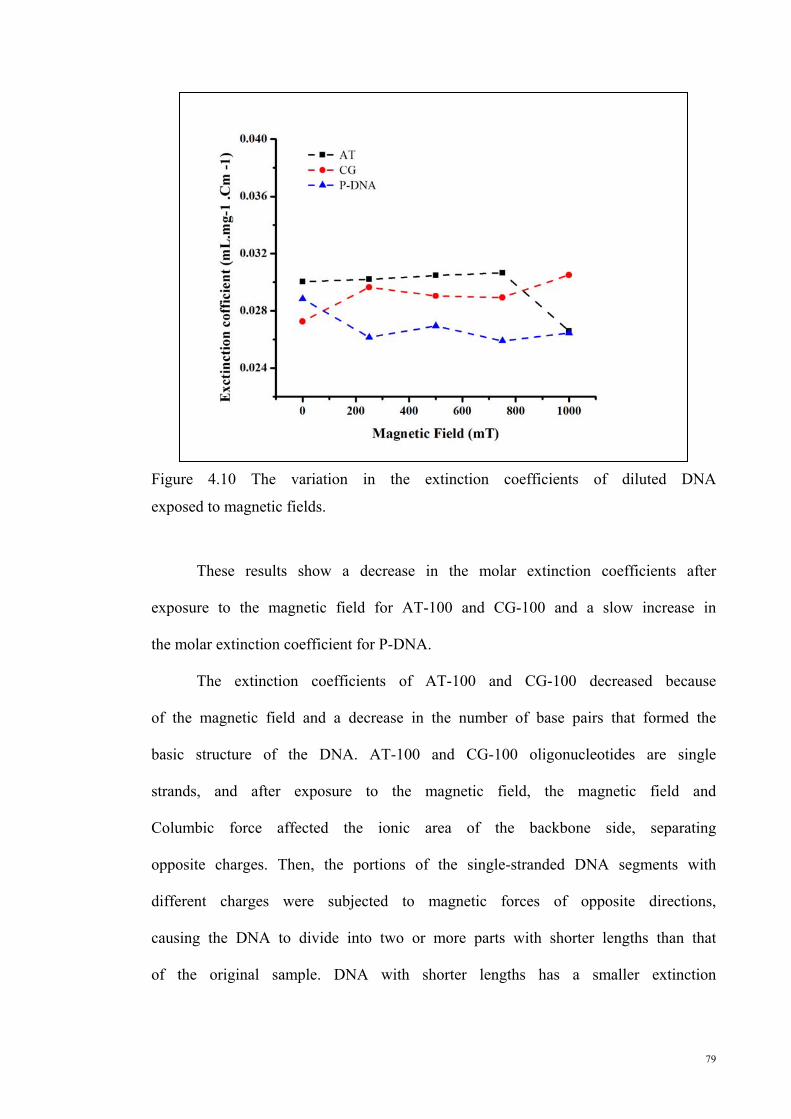
79

Figure 4.10 The variation in the extinction coefficients of diluted DNA

exposed to magnetic fields.

These results show a decrease in the molar extinction coefficients after

exposure to the magnetic field for AT-100 and CG-100 and a slow increase in

the molar extinction coefficient for P-DNA.

The extinction coefficients of AT-100 and CG-100 decreased because

of the magnetic field and a decrease in the number of base pairs that formed the

basic structure of the DNA. AT-100 and CG-100 oligonucleotides are single

strands, and after exposure to the magnetic field, the magnetic field and

Columbic force affected the ionic area of the backbone side, separating

opposite charges. Then, the portions of the single-stranded DNA segments with

different charges were subjected to magnetic forces of opposite directions,

causing the DNA to divide into two or more parts with shorter lengths than that

of the original sample. DNA with shorter lengths has a smaller extinction

80

coefficient, which decreased upon exposure to the magnetic field due to the

resultant short strands.

Application of magnetic field to the double-stranded DNA (P-DNA)

changed the DNA to single strands, and the DNA strands were cleaved

(Miyakoshi J, 2000). DNA cleavage is an important process in all living cells.

The general mechanism of DNA hydrolysis involves a type of nucleophilic

attack on the phosphate side of the DNA helix. Cleavage results from scission

of either the 3’-PO or the 5’-PO. In the presence of a magnetic field, an

activated hydroxide (Hydroxide ion will be accelerated by the magnetic field

and will act as activated hydrogen ) attacks the phosphate group, as shown in

the right side of Figure 4.11, and the leaving group will promote the

continuation of this process. The mechanism for cleavage is based on the

promoted 3’-PO scission. Increasing the extinction coefficient is considered a

hypochromic effect (biological perspective) that could increase the UV

absorbance of DNA as a result of the separation of two strands.

Figure 4.11 Mechanism of the hydrolysis interaction in the DNA helix.

http://en.wikipedia.org/wiki/UV

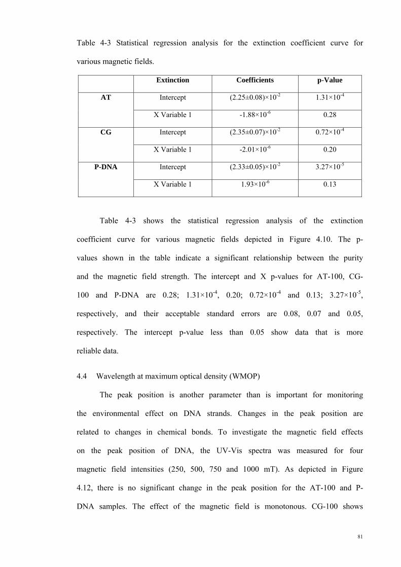
81

Table 4-3 Statistical regression analysis for the extinction coefficient curve for

various magnetic fields.

Extinction Coefficients p-Value

AT

Intercept (2.25±0.08)×10-2 1.31×10-4

X Variable 1 -1.88×10-6 0.28

CG

Intercept (2.35±0.07)×10-2 0.72×10-4

X Variable 1 -2.01×10-6 0.20

P-DNA

Intercept (2.33±0.05)×10-2 3.27×10-5

X Variable 1 1.93×10-6 0.13

Table 4-3 shows the statistical regression analysis of the extinction

coefficient curve for various magnetic fields depicted in Figure 4.10. The p-

values shown in the table indicate a significant relationship between the purity

and the magnetic field strength. The intercept and X p-values for AT-100, CG-

100 and P-DNA are 0.28; 1.31×10-4, 0.20; 0.72×10-4 and 0.13; 3.27×10-5,

respectively, and their acceptable standard errors are 0.08, 0.07 and 0.05,

respectively. The intercept p-value less than 0.05 show data that is more

reliable data.

4.4 Wavelength at maximum optical density (WMOP)

The peak position is another parameter than is important for monitoring

the environmental effect on DNA strands. Changes in the peak position are

related to changes in chemical bonds. To investigate the magnetic field effects

on the peak position of DNA, the UV-Vis spectra was measured for four

magnetic field intensities (250, 500, 750 and 1000 mT). As depicted in Figure

4.12, there is no significant change in the peak position for the AT-100 and P-

DNA samples. The effect of the magnetic field is monotonous. CG-100 shows

82

a slight increase from 254 to 257 nm. Guanine base pairs have a positive

susceptibility and less ionisation potential compared to those of the other bases.

In CG-100, 50% of the bases are G. The smallest ionisation potential of the

DNA bases is for guanine (Kawanishi, HirakuOikawa, 2001). The peak

position was related to the magnetic field effect on the HOMO and LUMO

states that changed by change in overlapping orbital's.

Figure 4.12 Variation of the maximum wavelength in the absorption spectra of

diluted DNA influenced by magnetic field exposure.

Table 4-4 shows the statistical regression analysis of the maximum

wavelength for various magnetic field strengths, which is also depicted in

Figure 4.12.The p-values shown in the table indicate a significant relationship

between the purity and the magnetic field strength. Intercepts and X p-values

for AT-100, CG-100 and P-DNA are 7.1×10-9; 0.157, 6.54×10-8; 1.00 and

5.38×10-8; 0.58 with acceptable accuracy.

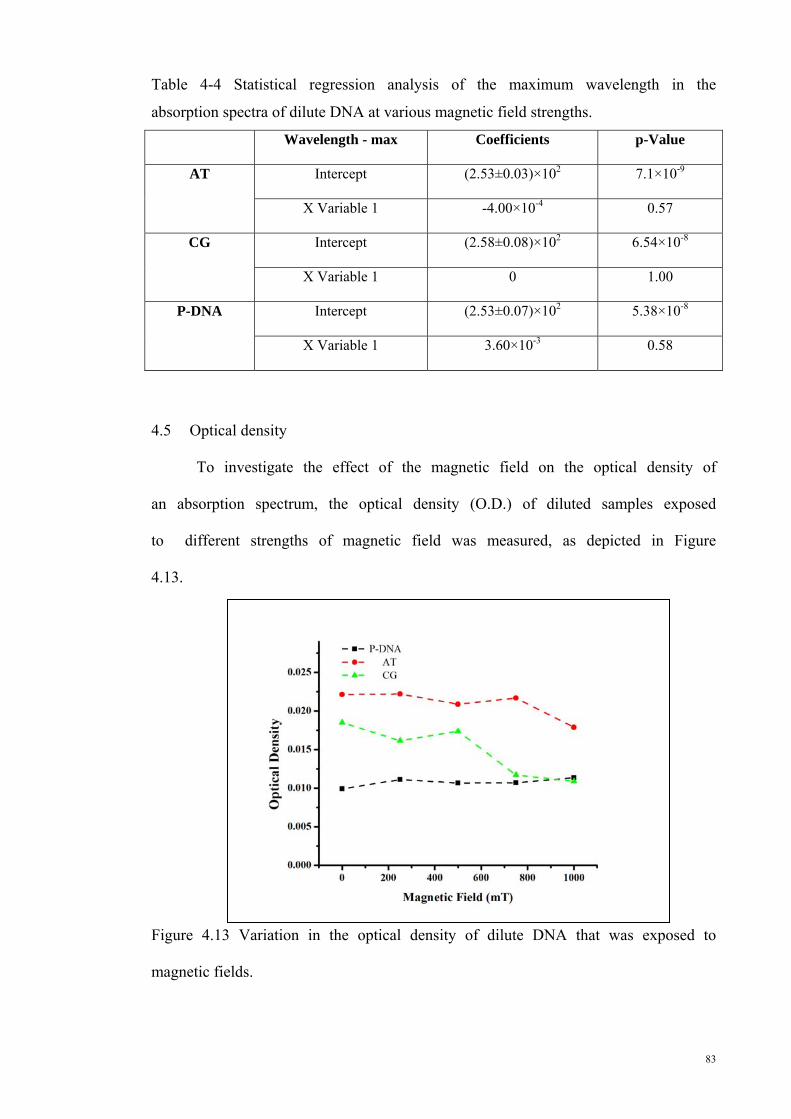
83

Table 4-4 Statistical regression analysis of the maximum wavelength in the

absorption spectra of dilute DNA at various magnetic field strengths.

Wavelength - max Coefficients p-Value

AT

Intercept (2.53±0.03)×102 7.1×10-9

X Variable 1 -4.00×10-4 0.57

CG

Intercept (2.58±0.08)×102 6.54×10-8

X Variable 1 0 1.00

P-DNA

Intercept (2.53±0.07)×102 5.38×10-8

X Variable 1 3.60×10-3 0.58

4.5 Optical density

To investigate the effect of the magnetic field on the optical density of

an absorption spectrum, the optical density (O.D.) of diluted samples exposed

to different strengths of magnetic field was measured, as depicted in Figure

4.13.

Figure 4.13 Variation in the optical density of dilute DNA that was exposed to

magnetic fields.

84

Figure shows that the O.D. of DNA, which is related to the concentration,

slightly decreased when exposed to high magnetic field of 750 mT.

Table 4-5 Statistical regression analysis of the optical density at various

magnetic field strengths.

O.Dmax Coefficients p-Value

AT

Intercept (2.28±0.1) ×10-2 1.73 ×10-4

X Variable 1 3.61 ×10-6 0.19

CG

Intercept (1.89 ±0.01) ×10-2 6.83 ×10-4

X Variable 1 -7.87 ×10-6 0.33

P-DNA

Intercept (1.02 ±0.04) ×10-2 8.88 ×10-5

X Variable 1 1.00 ×10-6 0.18

Optical density of AT-100 and CG-100 decreased after exposure to

magnetic field, and that of P-DNA increased. The explanation for the

extinction coefficient also applies for the optical density; the P-DNA was

cleaved after exposure to the magnetic field. Cleavage increased the absorption

of light and the optical density.

Table 4-5 show the statistical regression analysis for optical density at

various magnetic field strengths, which is also depicted in Figure 4.13. The p-

values in the table indicate a significant relationship between the purity and

magnetic field strength. Intercepts and X p-values for AT-100, CG-100 and P-

DNA are 1.73 ×10-4; 0.19, 6.83 ×10-4; 0.33 and 8.88 ×10-5; 0.18 with

acceptable accuracy.

85

5.1 CHAPTER V: RESULTS AND DISCUSSIONS:

PHYSICS PERSPECTIVE

5.1 Introduction

In this section, the physical properties of DNA samples exposed to

different magnetic fields were studied using techniques such as UV-Vis

analysis, Raman spectroscopy, temperature analysis and resistance monitoring.

Typically, the spectral absorbance measurements can be used in conjunction

with Beer-Lambert’s law, Kramers-Kronig rules and the Lorentz force to

calculate band gap, refractive index, loss function, chemical bond shifting,

temperature and resistivity.

5.1.1 Optical parameter

Numerous optical studies have been performed using deoxyribonucleic

acid at a variety of wavelengths. Optical properties, such as the band gap,

refractive index (n and k) and loss function are known. The band gap

calculations use direct band gap analysis, and the loss function and the

imaginary and real parts of the refractive index are derived using the Kramers-

Kronig method.

5.1.1.1 Band gap

Optical absorption of semiconductors is smallest for light with energies

less than the band gap and strong for larger energies. Therefore, there is a sharp

increase in absorption at wavelengths close to the band gap. Aqueous

suspensions of DNA were utilised to investigate the band gap using UV

absorption spectra. Absorption spectra were fitted by the equations for direct

86

band gap transitions. The equation to measure the direct band gap was

explained in Chapter 3 and its proof shown in APPENDIX A.

For a direction transition, (αE-photo)2 versus E-photo is used, where the

absorption coefficient and photon energy are α and E-photo, respectively. The

E-photo value extrapolated in the curve corresponds to a band gap Eg. Figures

5.1, 5.2 and 5.3 show the (αE-photo)2 versus E-photo profiles that were used

to calculate the cut-off wavelengths. Cut-off wavelengths can be estimated by

obtaining the intersection of the tangent line with the wavelength axis based on

Eq 5.1 and 5.2. This wavelength is usually used to determine the value of the

band gap value.

Eq 5.1

Eq 5.2 .)()(,

.0)(,

21

gg

g

EE

E

−∝>

=<

ωωαω

ωαω

hhh

hh

Interaction with higher light energy, in the UV and visible range of the

electromagnetic spectrum, causes DNA molecules and many other organic

materials to undergo transitions and electronic jumps between energy levels.

Upon absorption of the energy of UV or visible irradiation by an atom or a

molecule, electrons travel from lower to higher energy level of the molecular

orbitals.

Figures 5.1, 5.2 and 5.3 show the UV-Vis spectra of three samples

exposed to different magnetic fields. The peak shape of the three samples

clearly shows that the absorption spectra exhibit a tail that is beyond the band-

gap region; this tail indicates that the cut-off is not a sharp transition. This tail

Io) / (I log - = T log- =A , Io / I = T

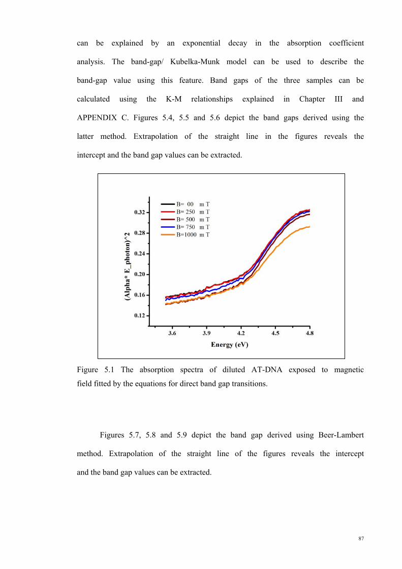
87

can be explained by an exponential decay in the absorption coefficient

analysis. The band-gap/ Kubelka-Munk model can be used to describe the

band-gap value using this feature. Band gaps of the three samples can be

calculated using the K-M relationships explained in Chapter III and

APPENDIX C. Figures 5.4, 5.5 and 5.6 depict the band gaps derived using the

latter method. Extrapolation of the straight line in the figures reveals the

intercept and the band gap values can be extracted.

Figure 5.1 The absorption spectra of diluted AT-DNA exposed to magnetic

field fitted by the equations for direct band gap transitions.

Figures 5.7, 5.8 and 5.9 depict the band gap derived using Beer-Lambert

method. Extrapolation of the straight line of the figures reveals the intercept

and the band gap values can be extracted.

88

Figure 5.2 The absorption spectra of diluted CG-DNA exposed to magnetic

field fitted by the equations for direct band gap transitions.

Figure 5.3 The absorption spectra of diluted P-DNA exposed to a magnetic

field were fitted by the equations for direct band gap transitions.

89

Table 5-1 compares the Eg values extracted from two methods; Beer-

Lambert and Kubelka-Munk methods. The Kubelka-Munk method involves

shorter wavelengths than the band gap energy that is directly obtained from the

absorption spectrum using the direct band gap method. Additionally, the two

methods show similar results. Band gaps were found to generally increase in

the samples. The contraction caused by the Lorentz force and the liquid

environment is largely based on dipole-dipole and free charge interactions that

could cause significant differences between their magnitudes. Interactions

between biological samples and static magnetic field occur via bounded ion

dynamics.

Figure 5.4 Kubelka-Munk coefficients of the absorption spectra of AT-DNA

exposed to various magnetic fields.

90

Figure 5.5 Kubelka-Munk coefficients of the absorption spectra of CG-DNA


Figure 5.6 Kubelka-Munk coefficients of the absorption spectra of P-DNA


91

The oscillation of a bound ion about its binding portion in a signalling

molecule can affect ionic transport. Overlap of the base molecular orbitals lead

to a decrease in the absorbance of UV light. Indeed, cleavage decreased the

overlap of the orbitals and the liberated dsDNA molecules are no longer

stacked as they were in dsDNA. Thus the orbital overlap is minimised and the

UV absorbance increases.

Table 5-1 Comparison of the Eg values determined using two methods; Beer-

Lambert and Kubelka-Munk.

5.1.1.2 Real and imaginary part of refractive index

The refractive index of tissues/biomaterials is a fundamental parameter

used in optical diagnosis tests and laser treatments. In basic biomaterials, such

B=0 mT B=250 mT B=500 mT B= 50 mT B=1000 mT

Bee

r-L

ambe

rt AT 3.665±0.003 3.635±0.003 3.726±0.003 3.665±0.002 3.694±0.003

CG 3.850±0.07 3.859±0.004 3.747±0.005 4.124±0.005 4.211±0.007

P- DNA 3.860±0.007 3.944±0.008 3.929±0.005 3.918±0.006 3.917±0.006

Kub

elka

-Mun

k AT 3.625±0.007 3.602±0.003 3.702±0.003 3.636±0.003 3.636±0.003

CG 3.835±0.005 3.843±0.004 3.720±0.005 4.120±0.005 4.209±0.008

P- DNA 3.839±0.008 3.931±0.008 3.915±0.006 3.903±0.007 3.902±0.006

92

as DNA, blood plasma and protein, studies using optical methods indirectly

rather than directly attract a lot of attention. This attention was not only

because of its wide application in biomedicine and bioscience but the

combination of sensors and optical devices increased its potential applications

further. Kramers-Kronig method is a crucial tool for studying the imaginary

and real parts of the refractive index. This tool is broadly used in the optics of

liquids and solutions to derive the real and imaginary parts of the refractive

index (Houssier and Kuball, 1971; Pinchuk, 2004).

In damped simple harmonic oscillator model, n and k are the real and

imaginary parts of the complex refractive index respectively. The Kramers-

Kronig transformation has been commonly used to determine the dielectric

constant from normal-incidence absorption spectra. Eq 5.3 and 5.4 derived

from the Kramers-Kronig relationship show the real and imaginary parts of the

refractive index, which can be used to derive the dielectric constants ( )(1 ωε

and )(2 ωε ).

Eq 5.3

Eq 5.4

Figures 5.7, 5.8 and 5.9 show the real part ( in ), and Figures 5.10, 5.11

and 5.12 indicate the imaginary part of the refractive index ( rn ); these values

are derived from Eq 5.4 and 5.5. Figure 5.7 shows the real part of the refractive

index of AT-100 DNA. The real part of the refractive index of AT-DNA (as

shown in Figure 5.7) did not change significantly when exposed to magnetic

fields below 750 mT but clearly increased at energies above 4.14 eV.

02/1

12/12

22

1 /])[(21 εεεε ++=rn

02/1

12/12

22

1 /])[(21 εεεε −+=in

93

Figures 5.7, 5.8 and 5.9 show the dispersion curve of the real part of the

refractive index of AT-100 DNA, CG-100 DNA and P-DNA after exposure to

different magnetic field strengths. The real part of the refractive index of CG-

DNA showed no significant change when exposed to magnetic fields below

750 mT. Similarly for AT-100, the refractive index decreased when exposed to

magnetic fields of 750 mT at energies less than 4.14 eV (indicated by the arrow

in Figure 5.7) following an increase in the energy region above. Density of

liquid corresponds to the real part of the refractive index. As shown in Figures

5.7 and 5.8, for both single strand AT and CG samples, the density of DNA

liquid samples in high energy region increased. In low energy region

meanwhile, it decreased when exposed to magnetic field above 750 mT.

However, the number of short length DNA oligo suspended in the liquid

increased. This result indicates cleavage of the DNA oligonucleotide.

The real part of the refractive index of P-DNA (as shown in Figure 5.9)

decreased after exposure to magnetic fields, indicating decrease in liquid

density. It can be due to cleavage of DNA, as a result of exposure to increasing

strength of magnetic field and this can result in increase of distribution of ions

in the liquid.

94

Figure 5.7 Dispersion curves of real part of the refractive index of AT-100

DNA after exposure to different strengths of magnetic fields.

Figure 5.8 Dispersion curves of real part of the refractive index of CG-100

DNA after exposure to different strengths of magnetic fields.

95

Figure 5.9 Dispersion curves of real part of the refractive index of P-DNA after

exposure to different strengths of magnetic fields.

Imaginary part of the refractive index of the AT-100 DNA and CG-100

DNA (as shown in Figures 5.10 and 5.11, respectively) meanwhile decreased

when exposed to a magnetic field of 750 mT. The imaginary part of refractive

index is related to the extinction coefficient. Molar extinction coefficient and

imaginary part of refractive index decreased in AT-100 and CG-100. Shorter

length of oligo DNA has the smaller extinction coefficient. The result proved

that the imaginary part of refractive index and molar extinction coefficient

decreased upon exposure to magnetic field due to cleavage of DNA, creating

small lengths of oligomers.

96

Figure 5.10 Imaginary part of the refractive index of AT-100 DNA exposed to

magnetic fields.

Figure 5.12 shows the gradual increase of the imaginary part of the

refractive index of P-DNA when exposed to magnetic fields. The imaginary

part of refractive index corresponding to the molar extinction coefficient was

observed to increase because of cleavage of DNA strands to two single strands.

As a result of this cleavage, number of suspended chain in liquid environment

increased and therefore density of DNA increased.

97

Figure 5.11 Imaginary part of the refractive index of CG-100 DNA exposed to

magnetic fields.

Figure 5.12 Imaginary part of the refractive index of P-DNA exposed to

magnetic fields.

98

5.1.1.3 Loss function

Cells can repair some parts of DNA helix damaged by the environment.

Interaction between the environment and molecules depend upon the range of

the interaction. Energy required for this interaction includes two types of

forces. The forces, Coulombic and van der Waals affect the partial charge in a

DNA double helix in the opposite directions of nucleotide arrangement. The

van der Waals interactions depend on the dielectric function and the imaginary

frequency in the liquid conditions of the cellular environment. Loss function is

dependent on the imaginary part of the dielectric constant according to the

relationship in Eq 5.5.

Eq 5.5 .

The loss function was modelled using Lorentz fitting according to Eq

5.6. Parameters in this equation are y0, w, xc and A representing the offset, the

width of peak, the centre point of peak position on the x-axis and the area

under the peak curve, respectively. Two more parameters w and xc are

significant for the analysis using this fitting as in the equation below:

Eq 5.6

..........................

99

Figure 5.13 Loss function of AT-100 DNA exposed to different magnetic field

strengths.

Figure 5.14 Loss function of CG-100 DNA exposed to different magnetic field

strengths.

100

Figure 5.15 Loss function of P-DNA exposed to different magnetic field

strengths.

Loss functions of the three samples (AT-100, CG-100 and P-DNA) are

depicted in Figures 5.13, 5.14 and 5.15, respectively. The Lorentz fit

parameters for the loss functions of three samples (AT-100, CG-100 and P-

DNA) are summarised in Table 5-2.

As shown in Table 5-2, the value of xc increased slightly with stronger

magnetic fields. This change was from 4.83±0.01 to 4.97±0.01 for AT-100 and

from 4.84±0.01 to 4.87±0.01 for CG-100. The xc value for P-DNA decreased

slightly from 4.62±0.01 to 4.61±0.01. Peak width value, w, also increased, and

the peak was broader after the exposure to high magnetic field of 1000 mT.

This change was from 1.8±0.3 to 1.8±0.3 for AT-100 and from 8.7±0.3 to

10.1±0.9 for CG-100. Increase in the w value for P-DNA (2.9±0.3 to 3.4±0.8),

was greater than that for AT and CG.

101

Table 5-2 Lorentz fit parameters for the loss function of AT-100, CG-100 and

P-DNA.

Magnetic Field

Lorentz Parameter AT-100 CG-100 P-DNA

B=0 mT xc 4.83±0.01 4.84±0.01 4.62±0.01

w 1.8±0.3 8.7±0.3 2.9±0.3

B=250 mT xc 4.83±0.01 4.84±0.01 4.61±0.01

w 1.8±0.3 8.5±0.3 3.6±0.3

B=500 mT xc 4.85±0.01 4.84±0.01 4.62±0.01

w 2.1±0.3 8.8±0.3 2.0±0.3

B=750 mT xc 4.84±0.01 4.86±0.01 4.62±0.01

w 1.9±0.3 9.7±0.3 2.0±0.3

B=1000 mT xc 4.97±0.01 4.87±0.01 4.61±0.01

w 4.1±0.3 10.1±0.8 3.4±0.8

The peak width increased when the DNA samples were exposed to large

magnetic field. The harmonic vibrations between atoms and molecules were

disturbed by the large magnetic field creating non equilibrium condition. After

switching off the magnetic field, the vibration returned to new equilibrium

states due to the changes spring constants of these systems. This increased the

width of the peak. These results are explained based on the Lorentz model for

increase in band width.

102

5.1.2 Raman spectroscopy

Raman spectroscopy is a powerful technique to observe vibrational

modes in a system. A 514 nm Raman analysis was performed to investigate the

magnetic field effects on DNA strands. To increase and enhance the Raman

signals, a thin layer of gold of approximately 80 nm thickness was deposited

on a silicon surface before coating DNA (Yu, Guan, Qin et al., 2008). Figures

5.16, 5.17 and 5.18 compare the Raman spectra of AT-100, CG-100 and P-

DNA before and after magnetic field exposure (at approximately 1000 mT).

Figure 5.16 Comparison of the Raman spectra of AT-DNA before and after

exposure to magnetic field.

http://en.wikipedia.org/wiki/Spectroscopy

103

Figure 5.17 Comparison of the Raman spectra of CG-DNA before and after


Figure 5.18 Comparison of the Raman spectra of P-DNA before and after


104

Figures 5.16, 5.17 and 5.18 show that the intensity of peak in the 3000–

3500 cm-1 region representing hydrogen bonds which decreased significantly

after exposure to magnetic fields. Indeed, hydrogen bonds are the main feature

of the chemical structure of biomolecules measurable by Raman spectroscopy.

Hydrogen bond intensity decreased in the three samples but was stronger in P-

DNA than in the other two samples.

The hydrogen bonds between two strands decreased in the case of P-

DNA. This decrease is related to the breaking of the hydrogen bonding

between the two stands (Faulkner and Macrae, 2006). Although AT-100 and

CG-100 are single-stranded DNA and P-DNA is double-stranded, the hydrogen

bonds decreased because of cleavage as a result of scission in either the 3’-PO

or the 5’-PO. The hydroxide that was activated in the magnetic field attacked

the phosphate group; continuation of the process being promoted by the

removed group.

PO2 has an asymmetric stretching vibration mode at 1221cm-1. The 892

cm-1 vibration meanwhile belongs to the sugar-phosphate stretch (Alex and

Dupuis, 1989). For symmetric phosphate vibrations at 1221 cm-1, there is a

shift towards the high frequency direction in P-DNA. The intensity of this peak

for AT-100 and CG-100 decreased at approximately 1230-1240 cm-1 (Nafisi,

Kahangi, Azizi et al., 2007; Nafisi and Norouzi, 2009). Changes observed in

the bands represented a type of scission in either the 3’-PO or the 5’-PO and a

conformational change (Neault, Naoui, Manfait et al., 1996; Alex and Dupuis,

1989). Interactions between biological samples and a static magnetic field

occur via bound ion dynamics. Magnetic exposure increases the electrostatic

charge in hydrogen bonds at base pairs and the polarities of DNA. Increasing

the strength of a magnetic field induces charge accumulation and larger

105

electrostatic polarities. Different charges in the segments impose a Columbic

force and increase the strengths of the magnetic field-induced Lorentz force.

The oscillation of a bound ion about its binding portion in a signalling

molecule can affect the vibrational frequency. In addition, increases in the

magnetic field increases the Columbic force and breaks the hydrogen-bond

network, thus increasing the number of double helix that split and break.

5.1.3 Resistivity

Electrical resistivity is a property of ionic solutions that depends on the

charge and ion status in diluted DNA samples. It should be noted that the

concentration is the same for all samples. To investigate the variation in

resistivity after exposure to magnetic field, the effect of four magnetic field

strengths (250, 500, 750 and 1000 mT) on diluted DNA was measured. Figures

5.19, 5.20 and 5.21 show the resistivity of AT-100, CG-100 and P-DNA,

respectively, when exposed to magnetic fields. All figures show decrease in the

resistivity of DNA when exposed to magnetic fields.

106

Figure 5.19 Resistivity of AT-DNA exposed to magnetic fields.

Figure 5.20 Resistivity of CG-DNA exposed to magnetic fields.

Figure 5.21 Resistivity of P-DNA exposed to magnetic fields.

107

There is an exponential decrease in resistivity, which is fitted by Eq 5.7. The

variation in energy caused by the magnetic field exposure, )(BΔ , that results from the

Effect is approximately 1.02×10-4 eV. TkB (which is the thermal energy or Boltzmann

constant times temperature), or approximately 0.0256 eV.

Increasing the magnetic field applied to the three samples allows the

resistivity to be determined. The resistivity is not strong because of the low

energy of the magnetic field effect.

Eq 5.7 )/)(exp()( TkBBR BΔα

Table 5-3 Statistical regression analysis of the resistivity of AT-100 A exposed

to various magnetic fields.

Magnetic Field Trend Line Parameter Coefficients p-Value

B=0 mT

Intercept (1.80±0.02)×103 3.25×10-6

X Variable 1 2.67×10-1 0.37

B=250 mT

Intercept (1.80±0.02)×103 2.55×10-6

X Variable 1 2.39×10-1 0.40

B=500 mT

Intercept (1.80±0.07)×103 2.04×10-6

X Variable 1 2.25×10-1 0.38

B=750 mT

Intercept (1.80±0.01)×103 1.51×10-6

X Variable 1 2.22×10-1 0.31

B=1000 mT

Intercept (1.80±0.01)×103 1.40×10-6

X Variable 1 2.19×10-1 0.30

108

Table 5-4 Statistical regression analysis of the resistivity of CG-100 exposed to



B=0 mT

Intercept (1.80±0.01)×103 1.07×10-6

X Variable 1 2.03×10-1 0.29

B=250 mT

Intercept (1.80±0.01)×103 1.11×10-6

X Variable 1 2.00×10-1 0.31

B=500 mT

Intercept (1.80±0.01)×103 1.06×10-6

X Variable 1 1.98×10-1 0.30

B=750 mT

Intercept (1.80±0.01)×103 8.74×10-7

X Variable 1 2.02×10-1 0.25

B=1000 mT

Intercept (1.80±0.01)×103 1.39×10-6

X Variable 1 2.28×10-1 0.27

Table 5-5 Statistical regression analysis of the resistivity of P-DNA exposed to



B=0 mT

Intercept (1.80±0.01)×103 3.97×10-7

X Variable 1 2.17×10-1 0.96

B=250 mT

Intercept (1.80±0.05)×103 7.85×10-8

X Variable 1 2.17×10-1 0.21

B=500 mT

Intercept (1.80±0.09)×103 3.25×10-7

X Variable 1 2.12×10-1 0.88

B=750 mT

Intercept (1.80±0.06)×103 9.18×10-8

X Variable 1 2.09×10-1 0.27

Intercept (1.80±0.06)×103 1.01×10-7

109

Tables 5-3, 5-4 and 5-5 indicate the statistical regression analysis used

to find the coefficient parameters and p-values. The intercept p-values for AT-

100, CG-100 and P-DNA are in the order of 10-6, which is less than 0.05 show

a valuable range for analysis. The p-values indicate that there is a meaningful

relationship between the resistivity and the magnetic field exposure time.

The acceleration of charge carries causing an increase in temperature after

magnetic field exposure. Errors in this measurement are in the order of 10-9

based on the accuracy of the instrument.

5.1.4 Temperature

The effects of magnetic fields on DNA temperature were investigated to

understand ionic motion. Temperature increases as the ionic motion in a

magnetic field increases the kinetic energy. The temperature variation for

different magnetic fields was measured for all the three samples before and

after four different magnetic field exposure times; 100 s, 200 s, 300 s and 400

s. As shown in Figures 5.22, 5.23 and 5.24, the maximum variation recorded

was approximately 2.5-3.8°C (all sample was placed in cryostat cylinder to

shield environment effect and temperatureAs shown as Figures 3-10, 3-11).

However this temperature was not significant enough to change the

optical density and break the double-stranded DNA. Double-stranded DNA can

divide into two strands at a critical temperature of approximately 95°C. The

increased temperature found in this experiment was not enough to cleave the

DNA stands. Maximum temperature during 400 s of magnetic field exposure

for the three samples of DNA used in this work was evaluated. Temperature of

AT-100, CG-100 and P-DNA increased by 2.5, 3 and 3.8°C, respectively. Such

B=1000 mT X Variable 1 2.03×10-1 0.32

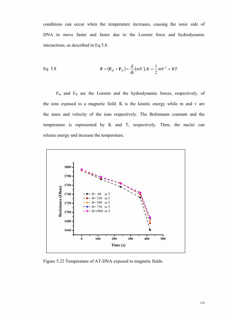
110

conditions can occur when the temperature increases, causing the ionic side of

DNA to move faster and faster due to the Lorentz force and hydrodynamic

interactions, as described in Eq 5.8.

Eq 5.8 ( ) ( ) KTmVKmVdtd

DM ===+= 2

21,FFF

Fm and FD are the Lorentz and the hydrodynamic forces, respectively, of

the ions exposed to a magnetic field. K is the kinetic energy while m and v are

the mass and velocity of the ions respectively. The Boltzmann constant and the

temperature is represented by K and T, respectively. Then, the nuclei can

release energy and increase the temperature.

Figure 5.22 Temperature of AT-DNA exposed to magnetic fields.

111

Figure 5.23 Temperature of CG-DNA exposed to magnetic fields.

Figure 5.24 Temperature of P-DNA exposed to magnetic fields.

112

Table 5-6 Statistical regression analysis of the temperature of AT-100 exposed


Magnetic

Field Trend Line Parameter Coefficients p-Value

B=0 mT

Intercept (2.39±0.01)×101 5.62×10-7

X Variable 1 4.94×10-3 0.29

B=250 mT

Intercept (2.39±0.01)×101 3.05×10-7

X Variable 1 4.97×10-3 0.15

B=500 mT

Intercept (2.39±0.01)×101 2.19×10-7

X Variable 1 5.15×10-3 0.10

B=750 mT

Intercept (2.39±0.09)×101 1.52×10-7

X Variable 1 5.16×10-3 0.71

B=1000 mT

Intercept (2.39±0.08)×101 1.10×10-7

X Variable 1 5.52×10-3 0.42

Table 5-7 Statistical regression analysis of the temperature of CG-100 exposed



B=0 mT

Intercept (2.43±0.03)×101 4.22×10-6

X Variable 1 8.56×10-3 0.43

B=250 mT

Intercept (2.42±0.02)×101 2.25×10-6

X Variable 1 6.82×10-3 0.45

B=500 mT

Intercept (2.43±0.04)×101 1.17×10-6

X Variable 1 5.34×10-3 0.30

B=750 mT

Intercept (2.44±0.03)×101 6.94×10-6

X Variable 1 5.16×10-3 0.26

B=1000 mT

Intercept (2.43±0.03)×101 4.22×10-6

X Variable 1 8.56×10-3 0.43

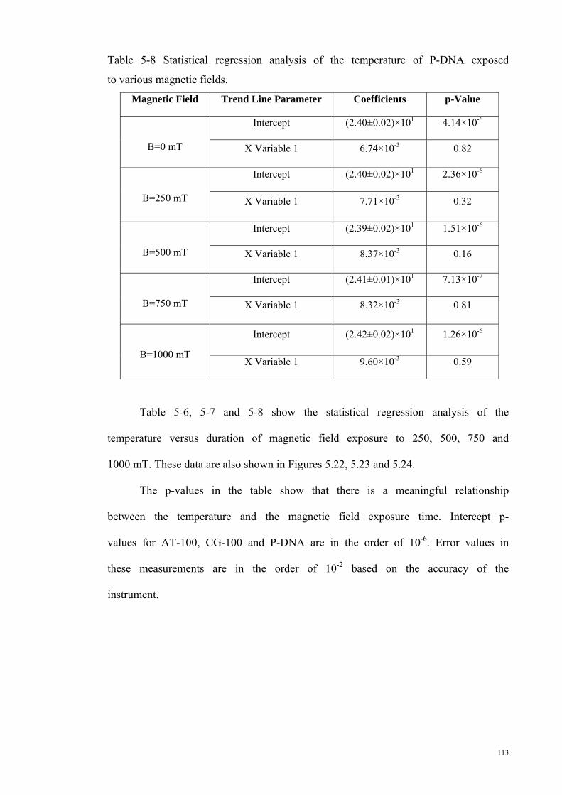
113

Table 5-8 Statistical regression analysis of the temperature of P-DNA exposed



B=0 mT

Intercept (2.40±0.02)×101 4.14×10-6

X Variable 1 6.74×10-3 0.82

B=250 mT

Intercept (2.40±0.02)×101 2.36×10-6

X Variable 1 7.71×10-3 0.32

B=500 mT

Intercept (2.39±0.02)×101 1.51×10-6

X Variable 1 8.37×10-3 0.16

B=750 mT

Intercept (2.41±0.01)×101 7.13×10-7

X Variable 1 8.32×10-3 0.81

B=1000 mT

Intercept (2.42±0.02)×101 1.26×10-6

X Variable 1 9.60×10-3 0.59

Table 5-6, 5-7 and 5-8 show the statistical regression analysis of the

temperature versus duration of magnetic field exposure to 250, 500, 750 and

1000 mT. These data are also shown in Figures 5.22, 5.23 and 5.24.

The p-values in the table show that there is a meaningful relationship

between the temperature and the magnetic field exposure time. Intercept p-

values for AT-100, CG-100 and P-DNA are in the order of 10-6. Error values in

these measurements are in the order of 10-2 based on the accuracy of the

instrument.

114

6.1 CHAPTER VI: CONCLUSIONS AND FUTURE WORKS

6.1 Introduction

The effects of magnetic fields of different strengths on plant based

DNA strands and oligonucleotide DNA were investigated in this work. DNA

and oligonucleotides of A-T and C-G were exposed to magnetic fields of

different strengths (0, 250, 500, 750 and 1000 mT) prior to characterizations

done using UV-Vis and Raman spectroscopy techniques along with

investigation on the resistivity and temperature profiles. The results were

analysed from the biological and Physics perspectives.


Analysis done from the biological perspectives based on the effects of

magnetic field strengths on DNA showed these results:

The effect of magnetic fields on DNA purity is not significant.

Magnetic field exposure increases the extinction coefficient of DNA

strands and decreases the extinction coefficient of oligonucleotide DNA.

Magnetic field exposure decreases the optical density of the three types

of DNAs used in this work.

Magnetic field exposure increases the wavelength of the DNA

absorption peak.

A significant observation obtained from these results showed that

the magnetic field exposure increased the DNA temperature and altered the

extinction coefficient. This significant influence of magnetic field resulted

in significant changes on DNA structure. Exposure to external magnetic

field not only broke the double-strand DNA into single strands but also cut

115

double- and single-stranded DNA into smaller lengths. However, these

effects did not change the purity of the DNA.


Analysis done from the Physics perspectives based on the effects of

magnetic field strengths on DNA showed these results:

Magnetic fields strength above 750 mT increased the band gap of DNA.

Magnetic fields strength above 750 mT changed the real part of the

refractive index of DNA by increasing and decreasing the index for

wavelengths below and above the absorption maximum respectively.

Magnetic field strengths above 750 mT decreased the imaginary part of

the refractive index of DNA.

Magnetic field strengths above 750 mT significantly affected the

hydrogen bonds in the DNA helix.

Resistivity of the three types of DNAs exposed to magnetic field

decreased.

The variation of DNA temperature exposed to external magnetic field

ranged from about 2-3.5°C in 10 minutes.

The effect of magnetic field effect on the band gap of DNA became

significant above 750 mT.

The results generally indicated that the effect of exposing DNA strands

and oligonucleotides to magnetic fields became significant for field strengths

above 750 mT. Band gap and refractive index changed because the electronic

orbital overlap decreased as a result of breakage of the DNA strands and the

splitting of energy levels after exposure to magnetic field. Results from Raman

spectroscopy, resistivity measurements and temperature monitoring were

116

comparable to those from UV-Vis spectroscopy for increasing magnetic field

intensities. Resistivity of the three types of DNAs exposed to magnetic fields

decreased due to division of the DNAs into smaller parts with cleavage

occurring at the ionic part. The ionic part increased conductivity and decreased

resistivity. Magnetic field increased charge acceleration and the resulting

collisions increased the temperature. The DNA temperature variation as a

result of exposure to magnetic field was approximately 2 to 3.5°C within 10

minutes. The effect of the magnetic field was evident in the Raman spectra as

observed by the disappearance or reduction of the hydrogen bond peaks. This

was in total agreement with the UV-Vis spectrum. Cleavage of DNA strands

and the breaking of the hydrogen bonds between the two strands also

corroborated with the UV-Vis and Raman spectra. Results show that the

magnetic field can be a useful tool for DNA analysis and manipulation and

therefore can be utilised to capture and analyse nanomaterials. The results also

show that the characterization and analysis carried out can be a useful

technique to evaluate environmental effect on biomolecules such as DNA.

Refractive index and band gap variation not only extend the application of

DNA in Physics and electronics but also opens up an avenue for possible

utilizations in biomedicine.

6.1.3 Future works

In the past few decades, applications of DNA (both as strands and

oligonucleotides) in Physics and as electronic devices have attracted significant

attention. Biological applications of this smart material also increased as a

result of this. The results achieved in this work, not only improved and

modified the previous applications of DNA as a smart material, but also have

provided a new perspective and highlighted more applications of DNA in

117

Physics and electronics. Temperature, resistivity and magnetic field sensors

using DNA as sensing material coupled to fibre optic sensors and microarray

structures are some possible interesting applications. Figure 6.1 summarises

the various potential applications of DNA that can be investigated for future

works based on the results and analysis done from both the Physics and

biological perspectives. Potential applications of this material are in electronic

devices such as sensors, arrays and other hybrid materials. The biological

applications of DNA can be further improved and previous applications can be

promoted to extend the capability of this material.

Figure 6.1 Potential applications of DNA strands and oligonucleotides in

Physics and Biology

.APPENDIX A

Applications Related to Physics

• Electronic Device• Fiber Optics• Micro array

• Detectors• Temperature• Magnetic• Resitivity

• Material• Liquid crystal• Microfluid• Liquid

Semiconductor

Applications Related to Biological

• Dignosis test• Defect and damage• Virous• Cancer

• Treatment• Protection • Drug • PCR• Purification

118

6.2 Light as an electromagnetic wave motion

An electromagnetic wave (EM-wave) is built up of oscillating electric

and magnetic fields. The waves oscillate in space and carries energy from one

place to another. Electric and magnetic field can be described as a harmonic

wave in the form:

Eq 6.1 ( )trkieEE ⋅−⋅⋅= ωrrr0

Eq 6.2 ( )trkieBB ⋅−⋅⋅= ωrrr0

The electric field Er

, magnetic field, Br

and propagation vector kr

, are

always mutually perpendicular). 0E and 0B represent their amplitudes, rr the

position and ω the angular frequency. If the wave is viewed at a fixed time,

the relation between the spatial wavelength, λ and the propagation constant k

can be found.

Eq 6.3 λπ2

=k

When viewing the wave at a fixed position, it is periodic in time with a

period, T. The relation between the propagation constant k, period T and the

wave velocityν, is:

Eq 6.4 π2=kvT

Both Er

and Br

satisfies a differential equation of the form:

119

Eq 6.5 2

2

22 1

tE

cE

∂∂

⎟⎠⎞

⎜⎝⎛=∇

In a direct band material, both the conduction band minimum and the

valence band minimum occur at the zone centre where k = 0.

In a indirect band gap material, the conduction band minimum does not

occur at k = 0, but is usually at the zone edge or close to it. The optical

absorption coefficient α ∝ Wi -> f transition rate (Fermi’s golden

rule).

Where

• the matrix element M,

• the density of states g(hω) (Eq 7.6) .

Eq 6.6

rdrHriHfM ifrrr 3* )(')(' ∫== ψψ

Eq 6.7

,' photone EpHrr

⋅−= , reperr

−=

Eq 6.8

rkiphoton eErE

rrrr⋅±= 0)( ,

rkierEerHrrrrr ⋅±⋅= 0)('

Eq 6.9

rkiii

ieruV

rrrrr ⋅= )(1)(ψ , rki

iiieru

Vr

rrrr ⋅= )(1)(ψ ,

).(2)( 2 ωπωα hgMh

W fi =∝ →h

120

Eq 6.10

rkiii

ieruV

rrrrr ⋅= )(1)(ψ

Eq 6.11

dkkgdEEg )(2)( = , dkkgdEEg )(2)( =

Eq 6.12

,/

)(2)(dkdEkgEg = 2

22

3 2)(4

)2(1)(

ππ

πkkgdkkdkkg =⇒=

Eq 6.13

rdrxuruM ifcellunitrrr 3* )()(∫∝

Eq 6.14

.

:

,)()()( 30

*

kkk

demandmomentumofonConservati

rderuerEeruVeM

if

rkii

rkirkif

rh

rh

rh

rrrrr rrrrrr

±=−

⋅= ⋅⋅±⋅−∫

Band gap calculation:

Eq 6.15

Eq 6.16

Eq 6.17

Eq 6.18

)()( kEkE VC −

).(2)( 2 ωπωα hgMh

W fi =∝ →h

.)(22

1)(

,0)(

212

3

2 gg

g

EforEg

Eforg

≥−⎟⎠⎞

⎜⎝⎛=

<=

ωωμπ

ω

ωω

hhh

h

hh

.221)( 2

123

*

2 EmEg ⎟⎟⎠

⎞⎜⎜⎝

⎛π

=h

121

Eq 6.19

.)()(,

.0)(,

21

gg

g

EEFor

EFor

−∝>

=<

ωωαω

ωαω

hhh

hh

Eq 6.20

.)(2

21)(

,0)(

212

3

2 gg

g

EforEg

Eforg

≥−⎟⎠⎞

⎜⎝⎛=

<=

ωωμπ

ω

ωω

hhh

h

hh

Eq 6.21

,/

)(2)(dkdEkgEg =

2

22

3 2)(4

)2(1)(

ππ

πkkgdkkdkkg =⇒=

Eq 6.22

Eq 6.23

Eq 6.24

..

,

*

22

22

22

22

2)(

2)(

2)(

2)(

soso

lhlh

hhhh

ege

mkkE

mkkE

mkkE

mkEkE

h

h

h

h

−Δ−=

−=

−=

+=

∗

∗

∗

*)(

*

22

)(

2222

1112

22

)()(

hlhe

g

hlheg

VC

mmwhere

kE

mk

mkE

kEkE

+=

+=

++=

−=

∗∗

μ

μ

ω

h

hh

h

.11,,

),(2

)()(

321

*3*2*1

2

−+=

+++=−

or

mk

mk

mkEkEkE

z

y

y

yxgVC

x

ηηη

ηηηh

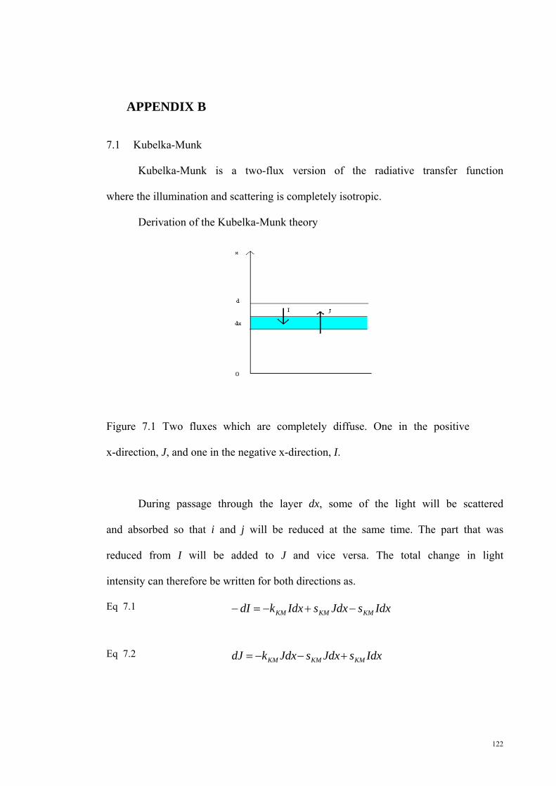
122

7.1 APPENDIX B

7.1 Kubelka-Munk

Kubelka-Munk is a two-flux version of the radiative transfer function

where the illumination and scattering is completely isotropic.

Derivation of the Kubelka-Munk theory

Figure 7.1 Two fluxes which are completely diffuse. One in the positive

x-direction, J, and one in the negative x-direction, I.

During passage through the layer dx, some of the light will be scattered

and absorbed so that i and j will be reduced at the same time. The part that was

reduced from I will be added to J and vice versa. The total change in light

intensity can therefore be written for both directions as.

Eq 7.1

IdxsJdxsIdxkdI KMKMKM −+−=−

Eq 7.2

IdxsJdxsJdxkdJ KMKMKM +−−=

123

sKM is the light scattering coefficient in m2/kg and kKM is the absorption

coefficient in m2/kg.

The mean path length for diffuse flux is 2 times the linear path length.

The Kubelka- Munk equations for diffuse light is

Eq 7.3

IdxsJdxsIdxkdI KMKMKM 222 −+−=−

Eq 7.4

IdxsJdxsJdxkdJ KMKMKM 222 +−−=

Setting K=2 kKM and S=2 sKM and re-arranging terms gives

Eq 7.5

( ) sJIsk

dxdI

++−=− , ( ) SIJSKdxdJ

++−=

Eq 7.6

a

SJS=

+ , JaISdxdI

+−=− , IaJSdxdJ

+−=

Eq 7.7

r

IJ= , 2i

jdiidjIJddr −

=⎟⎠⎞

⎜⎝⎛=

The approximation that light intensity is diffuse in both directions gives

the relation for reflectance over the differential layer dx.

Eq 7.8

∫ ∫=+−

⇒+−=R

Rg

w

dxSarr

drarrSdxdr

02

2

1212

Eq 7.9

12

)1)(1(

)1)(1(ln 2

22

22

−=−+−−−−

−+−−−−aSd

aaRaaR

aaRaaR

g

g

Eq 7.10

SK

SK

SKaa

aaR 211

11

2

22

2+−+=−−=

−+=∞

124

The reflectance for an opaque bulk can be determined by considering

an infinitely thick layer, ∞=d .Solving the equation for a finite layer gives

Eq 7.11

))/1(exp()/1()())/1(exp()/1())(/1(

∞∞∞∞

∞∞∞∞∞

−−−−∞−−−−

=RRSdRRRR

RRSdRRRRRRR

gg

gg

R0 is the reflectance of the sample over an ideally black background,

(Rg=0).

If one assumes that Rg=0.

Eq 7.12

∞∞∞∞

∞

−−−∞−

=RRRSdR

RRSdR

))/1(exp()/1(1))/1(exp(

0

Solving for S and by using the relation K=2 kKM and S=2 sKM.

Eq 7.13

⎟⎟⎠

⎞⎜⎜⎝

⎛−−−−

−=

∞∞

∞∞

∞

∞

))(1())((ln

)1( 2 RRRgRRgRRgR

RdRsKM

kKM can then be calculated using the relationship

Eq 7.14

∞

∞−=

RR

sk

KM

KM

2)1( 2

If the material is completely homogeneous, it is possible to use

grammage, w, instead of d.

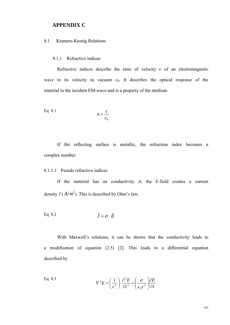
125

8.1 APPENDIX C

8.1 Kramers-Kronig Relations

8.1.1 Refractive indices

Refractive indices describe the ratio of velocity c of an electromagnetic

wave to its velocity in vacuum c0. It describes the optical response of the

material to the incident EM-wave and is a property of the medium.

Eq 8.1

0ccn =

If the reflecting surface is metallic, the refraction index becomes a

complex number.

8.1.1.1 Pseudo refractive indices

If the material has an conductivity σ, the E-field creates a current

density J ( 2/mA ). This is described by Ohm’s law.

Eq 8.2

EJrr

⋅= σ

With Maxwell’s relations, it can be shown that the conductivity leads to

a modification of equation (2.5) [2]. This leads to a differential equation

described by

Eq 8.3

tE

ctE

cE

∂∂

⎟⎟⎠

⎞⎜⎜⎝

⎛+

∂∂⋅⎟

⎠⎞

⎜⎝⎛=∇ 2

02

2

22 1

εσ

126

By combining the E-field as a harmonic wave with the differential

equation, it can be seen that the propagation vector, k, must be complex:

Eq 8.4

21

0

1 ⎥⎦

⎤⎢⎣

⎡⎟⎟⎠

⎞⎜⎜⎝

⎛+=

ωεσω i

ckr

The refractive index on the complex form can be derived as

Eq 8.5

21

0

1 ⎥⎦

⎤⎢⎣

⎡⎟⎟⎠

⎞⎜⎜⎝

⎛+=

ωεσinr

The refractive index can be written in general form:

Eq 8.6

ir nnn +=

where the real part, rnn =)Re( behave as the ordinary refractive index

and the imaginary part, Im(n)=ni determines the rate of absorption, α, in the

conductive medium.

Eq 8.7

The imaginary part, also known as extinction coefficient, is related to

the damping of the oscillation amplitude of the incident field.

A non-metallic material (dielectric) is a low absorbing material and the

imaginary part is small and often neglected. If the material is conductive, the

imaginary part is larger and must be taken into account.

λπ

α in4=

127

The amplitude reflectance (r) under irradiation and energy reflectance

(R) determined directly from the specular reflection spectrum are expressed by

the following equations:

Eq 8.8 √ √

Eq 8.9 | | .

Where, φ is the phase change. This results because both reflection and

absorption occur at the sample surface. r* is the complex conjugate of r.

Dividing Equation 9.8 into real and imaginary parts and solving for n and k

yields the following equations:

Eq 8.10 √

Eq 8.11 √√

Taking the logarithm of Equation (1), gives

Eq 8.12 √

However, √ and are not independent, but linked by Kramer's-

Kroning relationship:

Eq 8.13

If the energy reflectance is measured across the entire wavenumber

range, the phase change φ(νg) can be calculated at any required wavenumber

128

νg using this relational expression, and then the optical constants n and k can

be determined from Equations 9.12 and 9.13. Consequently, by calculating k at

constant wavenumber intervals across the normal infrared range between 4600

and 400 cm-1 for example, an absorbance coefficient spectrum equivalent to

the transmission spectrum can be calculated from the specular reflection

spectrum.

In the integration of Equation 9.13, a pole exists at ν = νg but several methods

have been proposed to handle this integration. Two typical methods are the

Maclaurin method and the double Fourier transform method. In the Maclaurin

method, the phase change φ(νg) is given by Equation 9.14

Eq 8.14 2 ∑

j = 2, 4, 6, ........., g-1, g+1, ......... (if g is an odd number)

j = 1, 3, 5, ........., g-1, g+1, ......... (if g is an even number)

The νj start point is set so that ν = νg does not occur and alternate data points

are used. With the double Fourier transform method, φ(νg) is determined by

Equation 9.14, a double Fourier transformation which is an approximation of

Equation 9.15.

Eq 8.15

4 2 √ 2

129

The Maclaurin method provides better calculation accuracy, but because

it is so time-consuming, the quicker double Fourier transformation method is

normally used.

130

9.1 APPENDIX D

9.1 Selection rules in Raman spectroscopy

22

0 0 0 20 0

0 0 0 00 0

0 0

1ˆf i f E i f x x E ix 2 x

f x E i f i f E i f x E ix x

0 0 E f x i E f x ix x

⎡ ⎤⎛ ⎞∂α ∂ α⎛ ⎞μ = μ + α = μ + α + + +⎢ ⎥⎜ ⎟⎜ ⎟∂ ∂⎝ ⎠⎢ ⎥⎝ ⎠⎣ ⎦⎡ ⎤∂α ∂α⎛ ⎞ ⎛ ⎞≈ μ + α + = μ + α +⎜ ⎟ ⎜ ⎟⎢ ⎥∂ ∂⎝ ⎠ ⎝ ⎠⎣ ⎦∂α ∂α⎛ ⎞ ⎛ ⎞= + + =⎜ ⎟ ⎜ ⎟∂ ∂⎝ ⎠ ⎝ ⎠

L

,

,

,

,

,,

,

,,

,

,

,

,

,

,

,

,

,

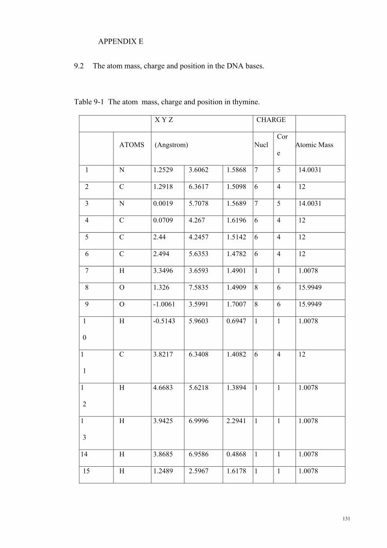
131

,APPENDIX E

9.2 The atom mass, charge and position in the DNA bases.

Table 9-1 The atom mass, charge and position in thymine.

X Y Z CHARGE

ATOMS (Angstrom) Nucl

Cor

e Atomic Mass

1 N 1.2529 3.6062 1.5868 7 5 14.0031

2 C 1.2918 6.3617 1.5098 6 4 12

3 N 0.0019 5.7078 1.5689 7 5 14.0031

4 C 0.0709 4.267 1.6196 6 4 12

5 C 2.44 4.2457 1.5142 6 4 12

6 C 2.494 5.6353 1.4782 6 4 12

7 H 3.3496 3.6593 1.4901 1 1 1.0078

8 O 1.326 7.5835 1.4909 8 6 15.9949

9 O -1.0061 3.5991 1.7007 8 6 15.9949

1

0

H -0.5143 5.9603 0.6947 1 1 1.0078

1

1

C 3.8217 6.3408 1.4082 6 4 12

1

2

H 4.6683 5.6218 1.3894 1 1 1.0078

1

3

H 3.9425 6.9996 2.2941 1 1 1.0078

14 H 3.8685 6.9586 0.4868 1 1 1.0078

15 H 1.2489 2.5967 1.6178 1 1 1.0078

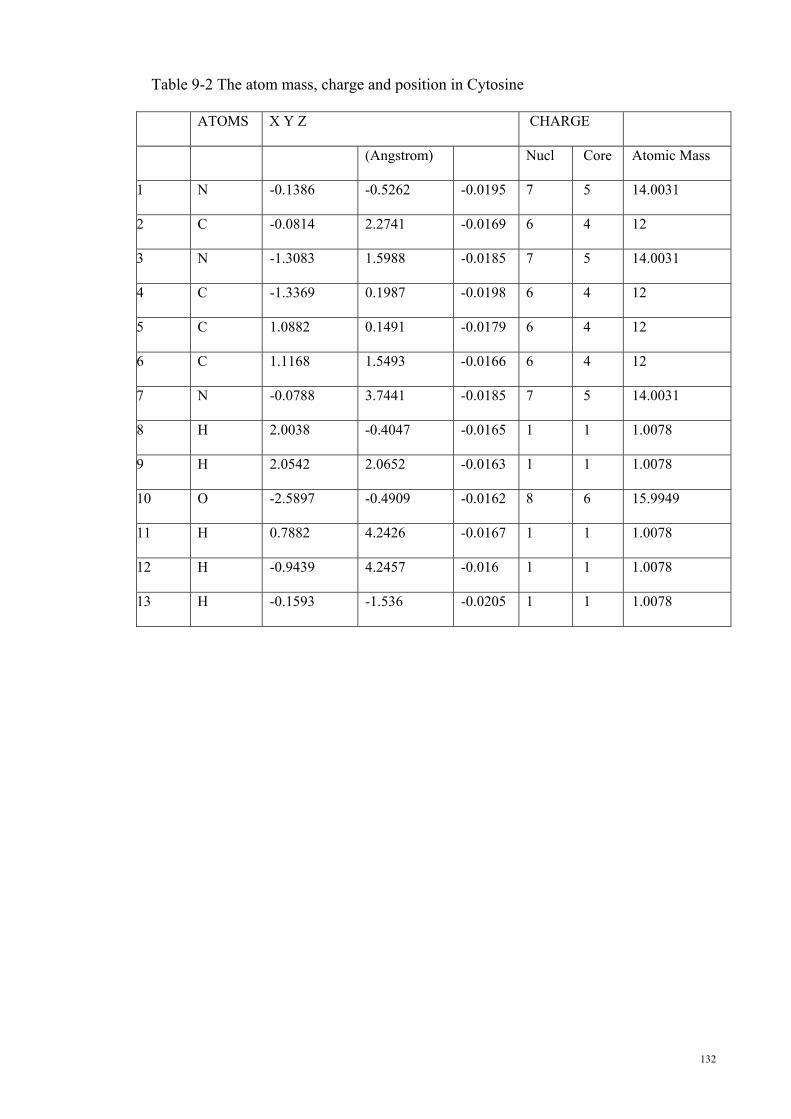
132

Table 9-2 The atom mass, charge and position in Cytosine

ATOMS X Y Z CHARGE

(Angstrom) Nucl Core Atomic Mass

1 N -0.1386 -0.5262 -0.0195 7 5 14.0031

2 C -0.0814 2.2741 -0.0169 6 4 12

3 N -1.3083 1.5988 -0.0185 7 5 14.0031

4 C -1.3369 0.1987 -0.0198 6 4 12

5 C 1.0882 0.1491 -0.0179 6 4 12

6 C 1.1168 1.5493 -0.0166 6 4 12

7 N -0.0788 3.7441 -0.0185 7 5 14.0031

8 H 2.0038 -0.4047 -0.0165 1 1 1.0078

9 H 2.0542 2.0652 -0.0163 1 1 1.0078

10 O -2.5897 -0.4909 -0.0162 8 6 15.9949

11 H 0.7882 4.2426 -0.0167 1 1 1.0078

12 H -0.9439 4.2457 -0.016 1 1 1.0078

13 H -0.1593 -1.536 -0.0205 1 1 1.0078

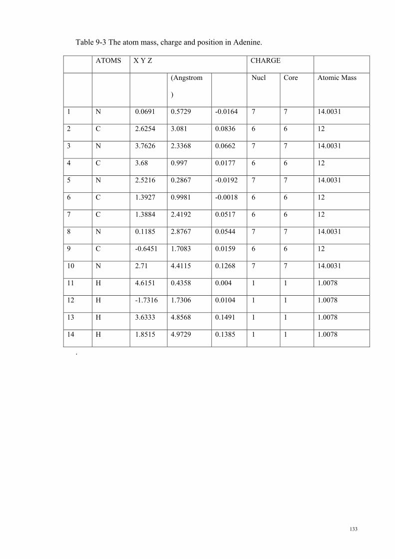
133

Table 9-3 The atom mass, charge and position in Adenine.

ATOMS X Y Z CHARGE

(Angstrom

)

Nucl Core Atomic Mass

1 N 0.0691 0.5729 -0.0164 7 7 14.0031

2 C 2.6254 3.081 0.0836 6 6 12

3 N 3.7626 2.3368 0.0662 7 7 14.0031

4 C 3.68 0.997 0.0177 6 6 12

5 N 2.5216 0.2867 -0.0192 7 7 14.0031

6 C 1.3927 0.9981 -0.0018 6 6 12

7 C 1.3884 2.4192 0.0517 6 6 12

8 N 0.1185 2.8767 0.0544 7 7 14.0031

9 C -0.6451 1.7083 0.0159 6 6 12

10 N 2.71 4.4115 0.1268 7 7 14.0031

11 H 4.6151 0.4358 0.004 1 1 1.0078

12 H -1.7316 1.7306 0.0104 1 1 1.0078

13 H 3.6333 4.8568 0.1491 1 1 1.0078

14 H 1.8515 4.9729 0.1385 1 1 1.0078

.

134

Table 9-4 The atom mass, charge and position in Guanine.

ATOMS X Y Z CHARGE

(Angstrom

)

Nucl Cor

e Atomic Mass

1 N -0.2445 1.8022 0.0362 7 5 14.0031

2 N 3.3546 3.6632 -0.0437 7 5 14.0031

3 C 3.313 2.2133 -0.0067 6 4 12

4 N 2.1226 1.5574 0.1238 7 5 14.0031

5 C 0.9818 2.2546 0.3342 6 4 12

6 C 0.9606 3.6817 0.3163 6 4 12

7 C 2.212 4.3977 0.0726 6 4 12

8 C -0.9802 2.9325 -0.1202 6 4 12

9 N -0.2767 4.0881 -0.0053 7 5 14.0031

10 O 2.235 5.6146 -0.0275 8 6 15.9949

11 N 4.4531 1.5025 -0.1446 7 5 14.0031

12 H -2.0309 2.913 -0.3771 1 1 1.0078

13 H 4.433 0.4582 -0.1352 1 1 1.0078

14 H 5.3717 1.985 -0.2604 1 1 1.0078

15 H 4.2668 4.1493 -0.2006 1 1 1.0078

16 H -0.5425 0.841 -0.0499 1 1 1.0078

135

REFERENCES Ahmad, M., Chang, K. P., King, T. A. and Hench, L. L. (2005). A compact

fibre-based fluorescence sensor. Sensors and Actuators, A: Physical,

119(1), 84-89.

Ahmadi, S. M., Dehghan, G., Hosseinpourfeizi, M. A., Dolatabadi, J. E. N. and

Kashanian, S. Preparation, characterization, and DNA Binding Studies

of Water-Soluble Quercetin Molybdenum (VI) Complex. DNA and Cell

Biology, 30(7), 517-523.

Alex, Serge and Dupuis, Paul. (1989). FT-IR and Raman investigation of

cadmium binding by DNA. Inorganica Chimica Acta, 157(2), 271-281.

Amara, S., Douki, T., Garrel, C., Favier, A., Rhouma, K. B., Sakly, M. and

Abdelmelek, H. Effects of static magnetic field and cadmium on

oxidative stress and DNA damage in rat cortex brain and hippocampus.

Toxicology and Industrial Health, 27(2), 99-106.

Amara, S., Douki, T., Garrel, C., Favier, A., Rhouma, K. B., Sakly, M. and

Abdelmelek, H. (2011). Effects of static magnetic field and cadmium on

oxidative stress and DNA damage in rat cortex brain and hippocampus.

Toxicology and Industrial Health, 27(2), 99-106.

Arbona, J. M., Aime, J. P. and Elezgaray, J. (2012). Folding of small origamis.

The Journal of Chemical Physics, 136, 3682472-3682479.

Atkins, Peter William and Friedman, Ron S. (1997). Molecular quantum

mechanics, New York: Oxford University Press, Oxford.

Banks, D. (2006). Microengineering, MEMS, and interfacing: A practical

guide, 199, United State: CRC Press.

Barnothy, Madeleine F. (1964). Biological effects of magnetic fields, New

York: Plenum Press.

136

Batson, PE and Silcox, J. (1983). Experimental energy-loss function, Im [-1/ε

(q, ω)], for aluminum. Physical Review B, 27(9), 5224–5239.

Blackman, CF, Benane, SG, Rabinowitz, JR, House, DE and Joines, WT.

(1985). A role for the magnetic field in the radiation‐induced efflux of

calcium ions from brain tissue in vitro. Bioelectromagnetics, 6(4), 327-

337.

Bodega, G., Forcada, I., Suárez, I. and Fernández, B. (2005). Acute and chronic

effects of exposure to a 1mT magnetic field on the cytoskeleton, stress

proteins, and proliferation of astroglial cells in culture. Environmental

Research, 98(3), 355-362.

Bosch, M. E., Sanchez, A. J. R., Rojas, F. S. and Ojeda, C. B. (2007). Recent

development in optical fiber biosensors. Sensors, 7(6), 797-859.

Bosch, M. E., Sánchez, A. J. R., Rojas, F. S. and Ojeda, C. B. (2007). Optical

chemical biosensors for high throughput screening of drugs.

Combinatorial Chemistry and High Throughput Screening, 10(6), 413-

432.

Brandes, Rolf and Kearns, David R. (1986). Magnetic ordering of DNA liquid

crystals. Biochemistry, 25(20), 5890-5895.

Braun, E., Eichen, Y., Sivan, U. and Ben-Yoseph, G. (1998). DNA-templated

assembly and electrode attachment of a conducting silver wire. Nature,

391(6669), 775-778.

Campàs, M. and Katakis, I. (2004). DNA biochip arraying, detection and

amplification strategies. TrAC - Trends in Analytical Chemistry, 23(1),

49-62.

Cantor, C. R., Warshaw, M. M. and Shapiro, H. (1970). Oligonucleotide

interactions. III. Circular dichroism studies of the conformation of

deoxyoligonucleolides. Biopolymers, 9(9), 1059-1077.

137

Cavaluzzi, M. J. and Borer, P. N. (2004). Revised UV extinction coefficients

for nucleoside5' monophosphates and unpaired DNA and RNA.

Nucleic Acids Research, 32(1), 1-9.

Chen, H., Fu, H., Zhu, X., Cong, P., Nakamura, F. and Yan, J. (2011).

Improved high-force magnetic tweezers for stretching and refolding of

proteins and short DNA. Biophysical Journal, 100(2), 517-523.

Collings, AF and Caruso, Frank. (1997). Biosensors: Recent advances. Reports

on Progress in Physics, 60(11), 1397-1445.

Cuniberti, Gianaurelio, Maciá, E, Rodriguez, A and Römer, RA. (2007). Tight-

binding modeling of charge migration in DNA devices. Charge

Migration in DNA, 1-20.

Davidson, Michael W, Strzelecka, Teresa E and Rill, Randolph L. (1988).

Multiple liquid crystal phases of DNA at high concentrations. Nature,

331, 457-460.

Dobson, Jon. (2008). Remote control of cellular behaviour with magnetic

nanoparticles. Nature Nanotechnology, 3(3), 139-143.

Dunn, David A, Lin, Vivian H and Kochevar, Irene E. (1992). Base-selective

oxidation and cleavage of DNA by photochemical cosensitized electron

transfer. Biochemistry, 31(46), 11620-11625.

El-Bialy, N. S. and Rageh, M. M. (2013). Extremely low-frequency magnetic

field enhances the therapeutic efficacy of low-dose cisplatin in the

treatment of ehrlich carcinoma. BioMed Research International, 2013,

1-7.

Eldashev, I. S., Shchegolev, B. F., Surma, S. V. and Belostotskaya, G. B.

(2010). Influence of low-intensity magnetic fields on the development

of satellite muscle cells of a newborn rat in primary culture. Biophysics,

55(5), 765-770.

138

Elson, E. (2009). I. the little explored efficacy of magnetic fields in cancer

treatment and postulation of the mechanism of action. Electromagnetic

Biology and Medicine, 28(3), 275-282.

Emura, R., Ashida, N., Higashi, T. and Takeuchi, T. (2001). Orientation of Bull

Sperms in Static Magnetic Fields. Bioelectromagnetics, 22(1), 60-65.

Epstein, J. R., Biran, I. and Walt, D. R. (2002). Fluorescence-based nucleic acid

detection and microarrays. Analytica Chimica Acta, 469(1), 3-36.

Faulkner, C. and Macrae, R. (2006). A DFT Study of Hydrogen

Bonding Between Adenine and Thymine. Proceedings of The Science,

Engineering and Mathematics Conference, University of Evansville, 1-11.

Fox, M. A. (1966). Biological effects of magnetic fields. Bulletin of

Mathematical Biology, 28(1), 137-138.

Gamboa, O. L., Gutierrez, P. M., Alcalde, I., De la Fuente, I. and Gayoso, M. J.

(2007). Absence of relevant effects of 5 mT static magnetic field on

morphology, orientation and growth of a rat Schwann cell line in

culture. Histology and Histopathology, 22(7-9), 777-780.

Ghasemifard, Mahdi, Zavar, Matineh, Ghasemifard, Hadi and Aliabad, Hossein

Asghar Rahnamaye. (2010). The effect of temperature dependences on

optical properties of PMN-PZT nano-powders. Journal of Optics, 39(4),

157-166.

Haber, Charbel and Wirtz, Denis. (2000). Magnetic tweezers for DNA

micromanipulation. Review of Scientific Instruments, 71(12), 4561-

4570.

Houssier, Glaude and Kuball, Hans‐G. (1971). Electro‐optical properties of

nucleic acids and nucleoproteins III. Kramers‐Kronig relationships in

linear birefringence and dichroism. Application to a DNA–proflavine

complex. Biopolymers, 10(12), 2421-2433.

139

Ichioka, S., Minegishi, M., Iwasaka, M., Shibata, M., Nakatsuka, T., Harii, K.,

Kamiya, A. and Ueno, S. (2000). High intensity static magnetic fields

modulate skin microcirculation and temperature in vivo.

Bioelectromagnetics, 21(3), 183-188.

Iguchi, Kazumoto. (2001). Semiconductivity and band gap of a double strand of

DNA. Journal of the Physics Society Japan, 70(2), 593-597.

Iwasaka, Masakazu and Ueno, Shoogo. (1998). Optical measurements of

magnetophoresis of macromolecules. Magnetics, IEEE Transactions on,

34(4), 2129-2131.

Jajte, Jolanta, Zmyslony, Marek, Palus, Jadwiga, Dziubaltwska, Elzbieta and

Rajkowska, Elzbieta. (2001). Protective effect of melatonin against in

vitro iron ions and 7 mT 50 Hz magnetic field induced DNA damage in

rat lymphocytes. Mutation Research/Fundamental and Molecular

Mechanisms of Mutagenesis, 483(1), 57-64.

Jangir, Deepak Kumar, Dey, Sanjay Kumar, Kundu, Suman and Mehrotra,

Ranjana. (2012). Assessment of amsacrine binding with DNA using

UV/visible, circular dichroism and Raman spectroscopic techniques.

Journal of Photochemistry and Photobiology B: Biology, 14, 38-43.

Jiang, Y. X., Lei, J. T. and Gao, X. F. (2006). Application of optical fiber DNA

biosensor. Chinese Journal of Clinical Rehabilitation, 10(41), 152-154.

Kawanishi, Shosuke, Hiraku, Yusuke and Oikawa, Shinji. (2001). Mechanism

of guanine-specific DNA damage by oxidative stress and its role in

carcinogenesis and aging. Mutation Research/Reviews in Mutation

Research, 488(1), 65-76.

Ke, W. Z., Yu, D. W., Gu, B. P. and Zhuang, Z. W. (2001). Raman

Spectroscopic Study of Microscopic Damage on the Space Structure of

DNA with Acetic Acid. Guang Pu Xue Yu Guang Pu Fen

Xi/Spectroscopy and Spectral Analysis, 21(6), 792-793.

140

Khatir, N. M., Banihashemian, S. M., Periasamy, V., Abd Majid, W. H. and

Rahman, S. A. (2012). Current-Voltage Characterization on Au-DNA-

Au Junctions under the Influence of Magnetic Field. Advanced

Materials Research, 535, 1350-1353.

Khatir, N. M., Banihashemian, S. M., Periasamy, V., Ritikos, R., Abd Majid,

W. H. and Rahman, S. A. (2012). Electrical Characterization of Gold-

DNA-Gold Structures in Presence of an External Magnetic Field by

Means of I-V Curve Analysis. Sensors, 12(3), 3578-3586.

Khatir, N. M., Banihashemian, S. M., Periasamy, V., Abd Majid, W. H. and

Rahman, S. A. (2012). DNA Strand Patterns on Aluminium Thin Films.

Sensors, 11(7), 6719-6727.

Kim, Jiyeon, Ha, Chang Seung, Lee, Hae June and Song, Kiwon. (2010).

Repetitive exposure to a 60-Hz time-varying magnetic field induces

DNA double-strand breaks and apoptosis in human cells. Biochemical

and Biophysical Research Communications, 400(4), 739-744.

Kimura, T., Takahashi, K., Suzuki, Y., Konishi, Y., Ota, Y., Mori, C., Ikenaga,

T., Takanami, T., Saito, R., Ichiishi, E., Awaji, S., Watanabe, K. and

Higashitani, A. (2008). The effect of high strength static magnetic fields

and ionizing radiation on gene expression and DNA damage in

Caenorhabditis elegans. Bioelectromagnetics, 29(8), 605-614.

Kirschvink, Joseph L, Kobayashi-Kirschvink, Atsuko and Woodford, Barbara J.

(1992). Magnetite biomineralization in the human brain. Proceedings of

the National Academy of Sciences, 89(16), 7683-7687.

Lai, Henry and Singh, Narendra P. (2004). Magnetic-field-induced DNA strand

breaks in brain cells of the rat. Environmental Health Perspectives,

112(6), 687-694.

Lan, Guo-Yu, Chen, Wei-Yu and Chang, Huan-Tsung. (2011). One-pot

synthesis of fluorescent oligonucleotide Ag nanoclusters for specific and

141

sensitive detection of DNA. Biosensors and Bioelectronics, 26(5), 2431-

2435.

Lee, Byung-Cheon, Johng, Hyeon-Min, Lim, Jae-Kwan, Jeong, Ji Hoon, Baik,

Ku Youn, Nam, Tae Jeong, Lee, Jung Ho, Kim, Jungdae, Sohn, Uy

Dong, Yoon, Gilwon, Shin, Sanghoon and Soh, Kwang-Sup. (2004).

Effects of extremely low frequency magnetic field on the antioxidant

defense system in mouse brain: a chemiluminescence study. Journal of

Photochemistry and Photobiology B: Biology, 73(1-2), 43-48.

Leszczynski, D. (2005). Rapporteur report: Cellular, animal and

epidemiological studies of the effects of static magnetic fields relevant

to human health. Progress in Biophysics and Molecular Biology, 87(2-3

), 247-253.

Leuba, S. H., Wheeler, T. B., Cheng, C. M., LeDuc, P. R., FernA, ndez-Sierra,

M. and Quiaones, E. (2009). Structure and dynamics of single DNA

molecules manipulated by magnetic tweezers and or flow. Methods,

47(3), 214-222.

Lin-Vien, Daimay. (1991). The handbook of infrared and Raman characteristic

frequencies of organic molecules. San Diego: Academic Press.

Lin, L. and Jiang, L. (2001). Molecule recognition and transducer technology of

DNA. Chemistry Bulletin/Huaxue Tongbao, 64(5), 261-267.

Lindqvist, Martina and Graslund, Astrid. (2001). An FTIR and CD study of the

structural effects of G-tract length and sequence context on DNA

conformation in solution. Journal of Molecular Biology, 314(3), 423-

432.

Lionnet, T., Allemand, J. F., Revyakin, A., Strick, T. R., Saleh, O. A.,

Bensimon, D. and Croquette, V. (2012). Single-molecule studies using

magnetic traps. Cold Spring Harbor Protocols, 1, 133-138.

142

Liu, X. and Tan, W. (1999). A fiber-optic evanescent wave DNA biosensor

based on novel molecular beacons. Analytical Chemistry, 71(22), 5054-

5059.

Mallidis, C., Wistuba, J., Bleisteiner, B., Damm, O. S., Groß, P., Wbbeling, F.,

Fallnich, C., Burger, M. and Schlatt, S. (2011). In situ visualization of

damaged DNA in human sperm by Raman microspectroscopy. Human

Reproduction, 26(7), 1641-1649.

Manosas, M., Meglio, A., Spiering, M. M., Ding, F., Benkovic, S. J., Barre, F.

X., Saleh, O. A., Allemand, J. F., Bensimon, D. and Croquette, V.

(2010). Chapter Thirteen-Magnetic Tweezers for the Study of DNA

Tracking Motors. Methods in Enzymology, 475, 297-320.

Marazuela, M. D. and Moreno-Bondi, M. C. (2002). Fiber-optic biosensors -

An overview. Analytical and Bioanalytical Chemistry, 372(5-6), 664-

682.

Martins, S. A. M., Prazeres, D. M. F., Fonseca, L. P. and Monteiro, G. A.

(2010). Optimization of DNA hybridization on aminopropyl-controlled

pore-glass particles: Detection of non-labeled targets by picogreen

staining. Analytical Letters, 43(17), 2694-2704.

McNamee, J. P., Bellier, P. V., McLean, J. R. N., Marro, L., Gajda, G. B. and

Thansandote, A. (2002). DNA damage and apoptosis in the immature

mouse cerebellum after acute exposure to a 1 mT, 60 Hz magnetic field.

Mutation Research/Genetic Toxicology and Environmental

Mutagenesis, 513(1-2), 121-133.

Mehrvar, M., Bis, C., Scharer, J. M., Moo-Young, M. and Luong, J. H. (2000).

Fiber-optic biosensors - Trends and advances. Analytical Sciences,

16(7), 677-692.

Minaichev, EV, Myasishcheva, GG, Obukhov, Yu V, Roganov, VS, Savel'Ev,

GI and Firsov, VG. (1970). Paschen--Back Effect for the muonium

atom. Journal of Experimental and Theoretical Physics, 58, 1586-1592.

143

Miyakoshi J, Yoshida M, Shibuya K, Hiraoka M. (2000). Exposure to strong

magnetic fields at power frequency potentiates X-ray-induced DNA

strand breaks. J Radiation Research, 41(3), 293-302.

Miyakoshi, Junji. (2006). The review of cellular effects of a static magnetic

field. Science and Technology of Advanced Materials, 7(4), 305-307.

Moore, R. L. (1979). Biological effects of magnetic fields: studies with

microorganisms. Canadian Journal of Microbiology, 25(10), 1145-

1151.

Morii, Nahoko, Kido, Giyuu, Suzuki, Hiroyuki, Nimori, Shigeki and Morii,

Hisayuki. (2004). Molecular chain orientation of DNA films induced by

both the magnetic field and the interfacial effect. Biomacromolecules,

5(6), 2297-2307.

Mosconi, F., Allemand, J. F., Bensimon, D. and Croquette, V. (2009).

Measurement of the torque on a single stretched and twisted DNA using

magnetic tweezers. Physical Review Letters, 102(7), 78301-78304.

Nafisi, Shohreh, Kahangi, Fatemeh Ghoreyshi, Azizi, Ebrahim, Zebarjad, Nader

and Tajmir-Riahi, Heidar-Ali. (2007). Interaction of zanamivir with

DNA and RNA: Models for drug DNA and drug RNA bindings. Journal

of Molecular Structure, 830(1-3), 182-187.

Nafisi, Shohreh and Norouzi, Zeinab. (2009). A Comparative Study on the

Interaction of Cis-and Trans-Platin with DNA and RNA. DNA and Cell

Biology, 28(9), 469-477.

Neault, J. F., Naoui, M., Manfait, M. and Tajmir-Riahi, H. A. (1996). Aspirin-

DNA interaction studied by FTIR and laser Raman difference

spectroscopy. FEBS Letters, 382(1-2), 26-30.

Niederberger, C. (2012). Re: In situ visualization of damaged DNA in human

sperm by raman microspectroscopy. Journal of Urology, 187(3), 995.

144

Niederberger, C. (2013). Re: Oxidative DNA damage in human sperm can be

detected by Raman microspectroscopy. Journal of Urology, 189(5),

1841.

Nielsen, Peter E, Jeppesen, Claus, Egholm, Michael and Buchardt, Ole. (1988).

Photochemical cleavage of DNA by nitrobenzamides linked to 9-

aminoacridine. Biochemistry, 27(17), 6338-6343.

Ohmi, Tadahiro. (1996). Total room temperature wet cleaning for Si substrate

surface. Journal of The Electrochemical Society, 143(9), 2957-2964.

Pan, H. and Liu, X. (2004). Apparent Biological Effect of Strong Magnetic

Field on Mosquito Egg Hatching. Bioelectromagnetics, 25(2), 84-91.

Peng, H. and Ling, X. S. (2009). Reverse DNA translocation through a solid-

state nanopore by magnetic tweezers. Nanotechnology, 20(18), 185101-

185116.

Perveen, F., Qureshi, R., Ansari, F. L., Kalsoom, S. and Ahmed, S. (2011).

Investigations of drug-DNA interactions using molecular docking,

cyclic voltammetry and UV-Vis spectroscopy. Journal of Molecular

Structure, 1004(1-3), 67-73.

Peter, C., Meusel, M., Grawe, F., Katerkamp, A., Cammann, K. and Borchers,

T. (2001). Optical DNA-sensor chip for real-time detection of

hybridization events. Analytical and Bioanalytical Chemistry, 371(2),

120-127.

Pinchuk, A. (2004). Optical constants and dielectric function of DNA's

nucleotides in UV range. Journal of Quantitative Spectroscopy and

Radiative Transfer, 85(2), 211-215.

Piunno, P. A. E., Hanafi-Bagby, D., Henke, L. and Krull, U. J. (2000). A

critical review of nucleic acid biosensor and chip-based oligonucleotide

array technologies. ACS Symposium Series, 762, 257-291.

145

Piunno, P. A. E., Watterson, J., Wust, C. C. and Krull, U. J. (1999).

Considerations for the quantitative transduction of hybridization of

immobilized DNA. Analytica Chimica Acta, 400(1-3), 73-89.

Potenza, L., Cucchiarini, L., Piatti, E., Angelini, U. and Dacha, M. (2004).

Effects of high static magnetic field exposure on different DNAs.


Potenza, Lucia, Ubaldi, Luca, De Sanctis, Roberta, De Bellis, Roberta,

Cucchiarini, Luigi and DachÃ , Marina. (2004). Effects of a static

magnetic field on cell growth and gene expression in Escherichia coli.

Mutation Research/Genetic Toxicology and Environmental

Mutagenesis, 561(1), 53-62.

Raylman, R. R., Clavo, A. C. and Wahl, R. L. (1996). Exposure to strong static

magnetic field slows the growth of human cancer cells in vitro.

Bioelectromagnetics Journal, 17, 358-363.

Richards, E. G. and Fasman, G. D. (1975). Handbook of Biochemistry and

Molecular Biology. Nucleic Acids. Cleveland: CRC Press.

Richter, J., Mertig, M., Pompe, W., Mönch, I. and Schackert, H.K. (2001).

Construction of highly conductive nanowires on a DNA template.

Applied Physics Letters, 78, 536-538.

Rogers, K. R. (2000). Principles of affinity-based biosensors. Applied

Biochemistry and Biotechnology - Part B Molecular Biotechnology,

14(2), 109-129.

Rogers, Kim R, Apostol, Alma, Madsen, Steen and Spencer, Charles W. (2001).

Fiber optic biosensor for detection of DNA damage. Analytica Chimica

Acta, 444(1), 51-60.

Saito, Samuel T., Silva, Givaldo, Pungartnik, Cristina and Brendel, Martin.

(2012). Study of DNA-emodin interaction by FTIR and UV/Vis

146

spectroscopy. Journal of Photochemistry and Photobiology B: Biology,

111, 59-63.

Sakurai, T., Terashima, S. and Miyakoshi, J. (2009). Effects of strong static

magnetic fields used in magnetic resonance imaging on insulin-secreting

cells. Bioelectromagnetics, 30(1), 1-8.

Salerno, D., Brogioli, D., Cassina, V., Turchi, D., Beretta, G. L., Seruggia, D.,

Ziano, R., Zunino, F. and Mantegazza, F. (2010). Magnetic tweezers

measurements of the nanomechanical properties of DNA in the presence

of drugs. Nucleic Acids Research, 38(20), 7089-7099.

Sekino, M., Tatsuoka, H., Yamaguchi, S., Eguchi, Y. and Ueno, S. (2006).

Effects of strong static magnetic fields on nerve excitation. IEEE

Transactions on Magnetics, 42(10), 3584-3586.

Shaw, C.P and Jirasek, A. (2009). The use of ultraviolet resonance raman

spectroscopy in the analysis of ionizing-radiation-induced damage in

DNA. Applied Spectroscopy, 63(4), 412-422.

Silaghi, S.D. (2005). Optical characterization of DNA bases on silicon surfaces.

PhD. Dissertation, Germany: University of Technology.

Singh, T. B., Sariciftci, N. S. and Grote, J. G. (2010). Bio-organic

optoelectronic devices using DNA. Organic Electronics Advances in

Polymer Science, 223, 189-212.

Slavicek, Petr, Winter, Bernd, Faubel, Manfred, Bradforth, Stephen E and

Jungwirth, Pavel. (2009). Ionization energies of aqueous nucleic acids:

photoelectron spectroscopy of pyrimidine nucleosides and ab initio

calculations. Journal of the American Chemical Society, 131(18), 6460-

6467.

Strick, TR, Allemand, JF, Bensimon, D, Bensimon, A and Croquette, V. (1996).

The elasticity of a single supercoiled DNA molecule. Science New York

Washington, 1835-1837.

http://link.springer.com/book/10.1007/978-3-642-04538-7

http://link.springer.com/bookseries/12

http://link.springer.com/bookseries/12

147

Teles, FRR and Fonseca, LP. (2008). Trends in DNA biosensors. Talanta,

77(2), 606-623.

Thachappillya Mukundan, Vineeth, Tran, Quang Minha Nhat and Tuona Phan,

Anh. (2013). Connecting magnetic micro-particles with DNA G-

quadruplexes. Soft Matter, 9(1), 216-223.

Theodosiou, Eirini and Thomas, Owen RT. (2008). On the application of

‘seeding’ techniques in the primary separation of plasmid DNA from

neutralised E. coli lysates. Journal of Chemical Technology and

Biotechnology, 83(2), 192-200.

Thompson, D. G., Enright, A., Faulds, K., Smith, W. E. and Graham, D. (2008).

Ultrasensitive DNA detection using oligonucleotide-silver nanoparticle

conjugates. Analytical Chemistry, 80(8), 2805-2810.

Tombelli, S., Mascini, M., Sacco, C. and Turner, A. P. F. (2000). A DNA

piezoelectric biosensor assay coupled with a polymerase chain reaction

for bacterial toxicity determination in environmental samples. Analytica

Chimica Acta, 418(1), 1-9.

Toyama, Akira, Miyagawa, Yoko, Yoshimura, Akari, Fujimoto, Naoko and

Takeuchi, Hideo. (2001). Characterization of individual adenine

residues in DNA by a combination of site-selective C8-deuteration and

UV resonance Raman difference spectroscopy. Journal of Molecular

Structure, 598(1), 85-91.

Ueno, S. (2012). Studies on magnetism and bioelectromagnetics for 45 years:

From magnetic analog memory to human brain stimulation and imaging.


Villarini, Milena, Moretti, Massimo, Scassellati-Sforzolini, Giuseppina,

Boccioli, Bruno and Pasquini, Rossana. (2006). Effects of co-exposure

to extremely low frequency (50 Hz) magnetic fields and xenobiotics

determined in vitro by the alkaline comet assay. Science of the Total

Environment, 361(1-3), 208-219.

148

Vo-Dinh, T, Alarie, JP, Isola, N, Landis, D, Wintenberg, Al L and Ericson,

MN. (1999). DNA biochip using a phototransistor integrated circuit.

Analytical Chemistry, 71(2), 358-363.

Walt, D. R. (2000). Bead-based fiber-optic arrays. Science, 287(5452), 451-452.

Wang, Hao, Lewis, James P and Sankey, Otto F. (2004). Band-gap tunneling

states in DNA. Physical Review Letters, 93(1), 016401-016404.

William Jr, D. (2007). Materials Science and Engineering: An introduction.

New York: John Wiley & Sons.

Witten, K. G., Bretschneider, J. C., Eckert, T., Richtering, W. and Simon, U.

(2008). Assembly of DNA-functionalized gold nanoparticles studied by

UV/Vis-spectroscopy and dynamic light scattering. Physical Chemistry

Chemical Physics, 10(14), 1870-1875.

Wolfbeis, O. S. (2004). Fiber-optic chemical sensors and biosensors. Analytical

Chemistry, 76(12), 3269-3284.

Xu, D. K., Ma, L. R., Liu, Y. Q., Jiang, Z. H. and Liu, Z. H. (1999).

Development of chemiluminescent biosensing of nucleic acids based on

oligonucleotide-immobilized gold surfaces. Analyst, 124(4), 533-536.

Yang, Xin, Wang, Xue-Bin, Vorpagel, Erich R and Wang, Lai-Sheng. (2004).

Direct experimental observation of the low ionization potentials of

guanine in free oligonucleotides by using photoelectron spectroscopy.

Proceedings of the National Academy of Sciences of the United States of

America, 101(51), 17588-17592.

Yang, Yuanlong, Celmer, Edward J, Koutcher, Jason A and Alfano, RR.

(2002). DNA and Protein Changes Caused by Disease in Human Breast

Tissues Probed by the Kubelka–Munk Spectral Function.

Photochemistry and Photobiology, 75(6), 627-632.

149

Yiming, Xu, Zhixiang, Zhou, Hongying, Yang, Yan, Xu and Zhiyi, Zhang.

(1999). Raman spectroscopic study of microcosmic photodamage of the

space structure of DNA sensitized by Yangzhou haematoporphyrin

derivative and Photofrin II. Journal of Photochemistry and

Photobiology B: Biology, 52(1-3), 30-34.

Yousef, T. A., Abu El-Reash, G. M., El-Gammal, O. A. and Bedier, R. A.

(2013). Synthesis, characterization, optical band gap, in vitro

antimicrobial activity and DNA cleavage studies of some metal

complexes of pyridyl thiosemicarbazone. Journal of Molecular

Structure, 1035, 307-317.

Yu, Q., Guan, P., Qin, D., Golden, G. and Wallace, P. M. (2008). Inverted size-

dependence of surface-enhanced Raman scattering on gold nanohole

and nanodisk arrays. Nano Letters, 8(7), 1923-1928.

Zai Qing, Wen and Thomas G.J, Jr. (1998). UV resonance raman spectroscopy

of DNA and protein constituents of viruses: Assignments and cross

sections for excitations at 257, 244, 238 and 229 nm. Biopolymers,

45(3), 247-256.

Zborowski, Maciej, Ostera, Graciela R, Moore, Lee R, Milliron, Sarah,

Chalmers, Jeffrey J and Schechter, Alan N. (2003). Red blood cell

magnetophoresis. Biophysical Journal, 84(4), 2638-2645.

Zhang, G., Zhou, Y., Yuan, J. and Ren, S. (1999). A chemiluminescence fiber-

optic biosensor for detection of DNA hybridization. Analytical Letters,

32(14), 2725-2736.

Zhou, J. H., Feng, Y. Y., Wu, X. H., Yang, H., Xing, W. and Lu, T. H. (2005).

Study on interaction between CT-DNA and cytochrome C using UV-Vis

spectroscopy and electrochemistry. Spectroscopy and Spectral Analysis,

25(8), 1306-1308.

150

Date post:	14-Jan-2017
Category:	Documents
Upload:	dokhanh
View:	222 times
Download:	1 times

SPECTROSCOPIC ANALYSIS OF DNA STRANDS INFLUENCED ...

Documents