Page 1
SPECTROSCOPIC MEASUREMENTS OF NATURAL AND ARTIFICIAL LIGHT
SOURCES
THESIS
Presented to the Graduate Council of
Texas State University-San Marcos
in Partial Fulfillment
of the requirements
for the Degree
Master of SCIENCE
by
Sagar Ghimire, M.S.
San Marcos, Texas
August, 2010
Page 2
SPECTROSCOPIC MEASUREMENTS OF NATURAL AND ARTIFICIAL
LIGHT SOURCES
Committee Members Approved:
____________________________
Karl D. Stephan, Chair
____________________________
Eulogio Velasco
____________________________
Wilhelmus J. Geerts
Approved:
____________________________
J. Michael Willoughby
Dean of the Graduate College
Page 3
COPYRIGHT
by
Sagar Ghimire
2010
Page 4
iv
ACKNOWLEDGEMENTS
I would like to thank my major advisor Dr. Karl D. Stephan for his guidance,
support and help throughout my master’s study. His expertise and experience made my
interest grew in the fields of plasma science and spectroscopy. I am also very thankful for
the innovative research environment he created in the laboratory. I would also like to
thank Dr. Velasco and Dr. Geerts for being on my committee and providing me with
constructive remarks and suggestions.
Our field experiment in the Marfa-Alpine areas would not have been completed
without help from Ms. Pamela Stephan and Mr. Benjamin Simons. I appreciate their
much needed logistical help. I also thank Mr. James Bunnell for helpful discussions.
I am very grateful to both the Department of Engineering Technology and the
Ingram School of Engineering for providing me with a graduate assistantship. I am
grateful to the Graduate College and the Associated Student Government for providing
me with scholarships. I am also thankful to my graduate advisor Dr. Batey for his
guidance.
I would like to thank my family for their support and love. Finally I am very
grateful to my wife Anita for her support.
This manuscript was submitted on March 25, 2010.
Page 5
v
TABLE OF CONTENTS
Page
ACKNOWLEDGEMENTS ............................................................................................... iv
ABSTRACT ..................................................................................................................... viii
CHAPTER
I. INTRODUCTION ................................................................................................1
II. METHODOLOGY ...............................................................................................6
Experiment I: Distance Estimation Using Oxygen Absorption Band ......................6
Experiment II: Atmospheric-Pressure DC Glow Discharge .................................13
Structure of the Normal Glow Discharge ...............................................................16
Temperature Measurement Using Emission Spectroscopy ....................................18
III. RESULTS ...........................................................................................................20
Experiment I ...........................................................................................................20
Experiment II ..........................................................................................................21
IV. ABSOLUTE CALIBRATION OF SPECTROSCOPIC SYSTEM ....................27
V. DISCUSSIONS ...................................................................................................31
REFERENCES ..................................................................................................................33
Page 6
vi
LIST OF FIGURES
Figure Page
1. Simplified system diagram of telescope-camera-spectrometer setup ..............................6
2. Headlight spectrum obtained on 24 May 2008 and corrected only for zero offset. .........8
3. Polynomial fit to the experimental data .........................................................................10
4. Comparison of the transmission function derived from experimental data and the
model transmission function of Pierluissi and Tsai for d=4.57 KM ...................11
5. Root-Mean-Squared Error for an object at approximately 4.57 km from the
observer ...............................................................................................................12
6. Experimental setup to produce DC atmospheric pressure normal glow discharge .......14
7. Basalt sample resting on disc electrode, supported beneath rod ....................................16
8. Structure of a DC glow discharge (it is “adapted from J. D. Cobine, Gaseous
Conductors (NY: Dover, 1958), fig. 8.4”) .........................................................17
9. Photo of 30-mm-long DC atmospheric-pressure normal glow discharge in air.
Current 5.1 mA, voltage 11.4 kV. Note pinkish positive column with two
stable striations, and numerous anode glows on surface of basalt in circle
approximately 18 mm in diameter. .....................................................................22
10. Room-light view of tungsten electrode and basalt surface ..........................................23
11. Modeled spectra and the corresponding best-fit for cathode glow (Trot = 1500 K,
Tvib = 3000 K)...................................................................................................24
12. Modeled spectra and the corresponding best-fit for positive column (Trot = 2500
K, Tvib = 2000 K) .............................................................................................25
Page 7
vii
13. Modeled spectra and the corresponding best-fit for anode glow (Trot = 500 K ,
Tvib = 3000 K ) .................................................................................................25
14. Fiber-optic cable directly connects LS-1-CAL unit with the spectrometer .................27
15. Re-imager over transit level used to take spectrum at different i
θ .............................28
16. Experimental setup to measure solid angle ..................................................................29
Page 8
viii
ABSTRACT
SPECTROSCOPIC MEASUREMENTS OF NATURAL AND ARTIFICIAL
LIGHT SOURCES
by
Sagar Ghimire, M.S.
Texas State University-San Marcos
August 2010
SUPERVISING PROFESSOR: KARL D. STEPHAN
A twenty-night field investigation at the site where reportedly Marfa lights
have most been observed was conducted. We made considerable progress in
developing a technique to identify false positives and to estimate their distance
based on the absorption of molecular oxygen at 762 nm band using the
spectroscopic data alone (Stephan, Ghimire, Stapleton, & Bunnell, 2009).
Spectroscopic studies of a type of glow discharge supported by natural porous rock
which covers relatively wide area of the rock, up to 2 cm in diameter, are presented.
The rotational, translational and vibrational temperatures of the discharge are
measured by comparing modeled optical emission spectra with spectroscopic
measurements from the discharge. Finally, an absolute calibration technique for our
spectroscopic system is presented.
Page 9
1
I. INTRODUCTION
Most naturally occurring light sources have been identified, extensively studied
and understood scientifically. Franklin studied the lightning phenomenon and proved that
it is a natural electrical discharge, and was able to reproduced lightning on a small scale
in the laboratory. Physicists were able to describe light’s behavior by using Maxwell’s
equations in a quantitative way. In the twentieth century, with the advent of the quantum
mechanics, understanding of how light is produced in nature was almost complete.
There are few natural occurring light-producing phenomena that lack a complete
comprehensive explanation which accounts for their unique characteristics and would
also permit their reproduction in the laboratory. One of the most well known of such
phenomena is ball lightning. People have reported seeing ball lightning for hundreds of
years (Abrahamson, Bychkov, & Bychkov, 2002). But scientists still can't explain what
causes it, or even exactly what it is. Although there have been numerous articles,
publications, and seminars on the phenomenon of ball lightning and fireballs, only a very
few have ever reported on the actual production of ball lightning. Yet even fewer of
these handfuls have ever actually produced fireballs under conditions that could be
considered similar to nature. There are thousands of witnesses who have seen ball
lightning and some people who have taken photographs. Another case of recurring
unexplained light phenomena are the so-called Marfa lights. Marfa lights are points or
spheroids of light that appear in a restricted geographical area between Marfa and Alpine,
Texas. These lights may or may not be related to ball lightning and are not as well
Page 10
2
accepted as an unexplained phenomenon compared to ball lightning. However, they are
more predictable in their occurrence. The only publication on this subject addressed
primarily to a scientific audience, before our twenty-night field investigation (Stephan, et
al., 2009), was a report of a two-night investigation carried out by the Society of Physics
Students at the University of Texas at Dallas (Stolyarov, Klenzig, Roddy, & Heelis,
2005).
Both Marfa lights and ball lightning studies so far lack good-quality experimental
and observational evidence mainly because of the following two reasons. First, scientific
data on natural ball lightning and Marfa lights are scarce owing to unpredictability. We
are unaware of any effort to obtain scientific data on ball lightning because the resources
required are very expensive. Also, most of the data gathered from eyewitness accounts
are not scientific as most of the witnesses are not scientifically trained observers. In the
case of Marfa lights there has been enough observational work done which suggests a
“true” Marfa light event occurs at most between two to three times in a year. This implies
that a long-term effort is required to collect the observational data. Secondly, the
available data are not of scientific quality. The photographs of ball lightning could not
even yield basic data about the spectral shape. This same problem occurs in the case of
Marfa lights.
In this thesis we have two different but related attempts to obtain quantitative
spectroscopic data that will enable us to theorize about the nature of ball lightning and
Marfa lights in a more disciplined and scientific way. Spectroscopy is the science of
using spectral analysis to figure out what something is made of. Spectra are very
powerful tools in studying astronomical objects and plasmas because they represent the
Page 11
3
signature pattern of the source of light. The light we see is composed of a mixture of
wavelengths. We can separate the light into its component wavelengths (spectrum) by
passing it through a dispersing element such as a diffraction grating or a prism. There are
two basic types of spectra: continuous spectra and line spectra. Continuous spectra
originate from heated solids such as the heated tungsten filament in incandescent light
bulbs. Line spectra originate from individual atoms such as in low pressure gas discharge
lamps. Line spectra are specific for a certain elements and provide us a means to
determine the atomic composition of the source.
The thesis is divided into two parts. In the first part, we describe a 20 night field
experiment conducted at the Marfa Light View Park, during which we obtained spectra of
several objects, such as automotive headlights, some of which could have been mistaken
for lights of unknown origin by casual observers. The Marfa lights are reported to be seen
in or near Mitchell Flat, an area between Alpine and Marfa in Texas (Bunnell, 2009).
Many people have reported seeing them. They are yellowish-white lights that glow, fade,
disappear, and return in different places (Hall, 2006) . Although we did not see any
“genuine” Marfa lights, spectroscopic analysis of the visible oxygen absorption band near
13121 cm-1
(762 nm) was used to derive an algorithm to estimate distances to automotive
headlights with a continuum spectrum (Stephan, et al., 2009). This technique can be used
to estimate distances to the false positives from the spectroscopic data alone. This
distance measuring algorithm could be used to estimate distance to other light sources of
unknown origin with a continuum spectrum as well.
The second part of the thesis describes a study of a type of glow discharge
supported by natural porous rock. One explanation for luminous objects that are excited
Page 12
4
by electric fields is called St. Elmo’s fire – a kind of corona discharge. Some eyewitness
accounts of ball lightning may be corona discharge; however, there is very little scientific
literature about the mechanism by which corona may appear visible on the surface of the
ground. We attempted to investigate this phenomenon experimentally in laboratory
settings. We discovered that many types of moist porous rocks support a type of DC glow
discharge that has been identified in laboratory settings with artificial materials.
However, it is not clear what are the conditions required for this type of normal glow
discharge to occur in nature. There has been considerable industrial interest in generating
large volume (diffuse) discharges at atmospheric pressure. Although these plasmas can be
produced between metal electrodes (Staack, Farouk, Gutsol, & Fridman, 2005), they are
typically small with diameter less than 200 µm. The most important observation that we
made regarding the glow discharges in porous rock is the fact that it covers a surface area
up to 2 cm in diameter. This is unprecedented in the literature and therefore we are in the
process of completing a paper on this matter. Also, from the spectroscopic analysis of the
glow discharges we have found that it is essentially a low-temperature plasma, which
may have useful applications in industries. A program called SPECAIR, which does
sophisticated modeling of atmospheric spectra, has been used to compare our
experimental results with the simulated model spectrum.
SPECAIR is a program for modeling the absolute intensity spectral radiation
emitted by gases and plasmas of various compositions. It can model 37 molecular
transitions as well as atomic lines of N,O, and C (Laux, Spence, Kruger, & Zare, 2003). It
lets us choose translational, electronic, vibrational and rotational temperatures
individually. The code then uses Boltzmann distributions of the electronic, vibrational,
Page 13
5
and rotational temperatures to determine the population of the internal energy levels.
SPECAIR also allow us to take into account the effect of absorption by room air between
the emitting gas or plasma and the detector.
An important issue discussed in this thesis is the calibration of our spectroscopic
system. Much effort is needed for the absolute calibration of the intensity axis. A relative
calibration takes into account only the spectral sensitivity of the spectroscopic system
along the wavelength axis. An absolute calibrated system provides calibrated spectra,
which gives direct access to plasma parameters (Fantz, 2006). Thus, our effort will be
rewarded by an increase in information. One of the most critical steps in the calibration
procedure is the imaging of the light source to the spectroscopic system. We must be very
careful to conserve the solid angle. Although our efforts to calibrate our spectrometer are
incomplete, we present a theoretical framework for carrying out such calibration in the
final portion of this thesis, along with some experimental data.
Page 14
6
II. METHODOLOGY
Experiment I: Distance Estimation Using Oxygen Absorption Band
A simplified system diagram is shown in Figure 1. Besides optical spectra, we
recorded video images of the object of interest with all data time-stamped with the
precise time data available from a GPS receiver (Stephan, et al., 2009).
Figure 1. Simplified system diagram of telescope-camera-spectrometer setup
The telescope is a Celestron CPC-800 Schmidt-Cassegrain design with a 203-mm
aperture. It was equipped with a 1-X finding sight and 8-X finding scope used for initial
sighting of objects of interest (see Figure 1). A splitter/imager system was attached to the
Page 15
7
visual back of the telescope. The splitter/imager used a 75%-reflectivity beamsplitter
mirror that directed most of the incoming light to two plano-convex lenses, which
focused the beam onto a 1-mm-diameter fiber-optic cable leading to an Ocean Optics
QE65000 CCD-array spectrometer. The spectrometer can produce a resolution of about 3
nm when resolving a single atomic line. The size of the image produced by the
splitter/imager on the fiber end was designed so that 50% or more of the peak on-axis
optical power from a point source would enter the fiber as long as the telescope was
pointed to within ±5 arcmin of the source. Since the video camera used a 1/3-inch chip
giving a field of view that was approximately 5 by 7.5 arcmin, the fiber image size
ensured that any luminous source visible through the camera could also produce a
spectrum, assuming its intensity was sufficient.
The spectrometer was monitored with a laptop computer. The telescope control
was manual, although an automatic tracking feature could easily be incorporated without
much additional hardware. Custom software was used to monitor azimuth and altitude
data from the telescope’s motorized elevation-azimuth mount every 0.7 seconds. The
position data were time stamped with GPS-synchronized time codes.
The spectrometer was set to capture spectrum covering the 200-900 nm range.
Exposure time of 10 seconds was found to be adequate for capturing spectrum of dim
objects without saturating the CCD on bright objects.
Page 16
8
Power sources were one of the important considerations for our field experiment
because commercial power was not available. We used a 12-V 110-AH deep-discharge
lead-acid battery. This allowed continuous operation of our setup for at least 5 hours.
Initially we used two 17-AH 12-V power packs using gel-type lead acid batteries, but
these proved to be inadequate.
Molecular oxygen has a spectroscopic absorption band near the 762 nm (13121
cm-1
) region as shown in Figure 2. This band was first noted by Fraunhofer in the solar
spectrum and is often referred to as the Fraunhofer A band.
Figure 2. Headlight spectrum obtained on 24 May 2008 and corrected only for zero
offset.
Page 17
9
Because the depth of the absorption “notch” caused by this band is a
monotonically increasing function of the optical depth of the atmosphere between the
source and the observer, it has been used for various remote-sensing purposes such as
determining cloud heights from satellites (Pierluissi & Tsai, 1986; Wark & Mercer,
1965). Sufficient absorption occurs in this band over path lengths as short as 1 km to
permit estimation of the source-to-observer distance of continuum sources. Our distance-
estimation algorithm is a two-step process.
In the first step, the experimental data points that lie outside absorption bands
were used to obtain a cubic polynomial ( )i
P υ fit to a small portion of the underlying
continuum spectrum as shown in Figure 3 (Stephan, et al., 2009). The cubic polynomial
model is our model for the source spectrum as it would appear to our spectrometer
without the absorption bands. We used this polynomial to transform our raw data into an
experimental transmission function EXP
τ whose value outside the absorption bands is
approximately unity. If the raw spectrometer data in counts per wavenumber pixel after
subtracting dark-spectrum background are designated as ( )i
D υ , then the experimental
transmittance function is
( )
( )( )
iEXP i
i
D
P
υτ υ
υ= (1)
The experimental transmission function for each of N=32 wavenumbers covering
the Fraunhofer A absorption band , specifically from 13267 cm-1
to 12870 cm-1
is
computed. These 32 data-points correspond to the 32 pixels provided by the QE65000
Page 18
10
spectrometer output in the selected band. The pixels are spaced about 0.75 nm apart in
this region.
Figure 3. Polynomial fit to the experimental data
Using expressions and tables derived by (Pierluissi & Tsai, 1986) for their model
of atmospheric transmittance in the A band, we used the variables of atmospheric
pressure, temperature, and optical path length to obtain a predicted or model transmission
function MOD
τ . Next, we adjusted the optical path length used in the model transmission
function until the root-mean-square error between the experimental and model
transmission functions was minimized. Figure 4 shows the modeled and the derived or
experimental transmission functions.
Page 19
11
Figure 4. Comparison of the transmission function derived from experimental data
and the model transmission function of Pierluissi and Tsai for d=4.57 KM
The path length that gives the minimum root-mean-square error between the two
functions is the estimated distance to the source. This is shown in Figure 4 (Stephan, et
al., 2009). The RMSE as a function of distance d can be expressed as
1/2
1
( ( , ) ( , )
( )
N
EXP i MOD i
i
d d
dN
τ υ τ υ
ε =
−
=
∑ (2)
Page 20
12
Figure 5. Root-Mean-Squared Error for an object at approximately 4.57 km from
the observer
This algorithm produces a reasonably accurate estimate of the optical path length,
which converts directly to distance if the atmospheric conditions are known. When a
source is known to be located on a road, its location can often be established
independently by means of GIS and azimuth data. In these cases we can compare the
distance calculated by the atmospheric oxygen-band absorption and GIS-azimuth
approaches. The RMSE in (2) as a function of distance d for an observation of headlights
on 24 May 2008 at 21:20:35 CDT is shown in Figure 5 (Stephan, et al., 2009). The
minimum value of RMSE is at 4.57 km.
The result of this experiment is presented in the results section later.
Page 21
13
Experiment II: Atmospheric-Pressure DC Glow Discharge
The generation of uniform glow discharges in open air is a remarkable
achievement in plasma field research. Uniform and stable glow discharges without
additional flowing gases and a vacuum chamber eliminate the need for low-pressure
technology and vacuum-compatible materials, and can be applied to plasma applications
such as surface modification, thin film deposition and etching used in the semiconductor
industry, cleaning, removing pollutant gases, and sterilization (Garamoon & El-zeer,
2009; Staack, et al., 2005).
One of the most studied non-equilibrium plasma discharge is the low pressure
normal glow discharge. We investigated the spectra of atmospheric pressure DC normal
glow discharge in air. The setup as shown in Figure 6 was used. The power supply was
connected in series to the ballast resistor and the discharge gap. When the power supply
voltage is in excess of the breakdown voltage for the gap the discharge initiates. The
ballast resistor of 400 kΩ serves to stop the current from increasing too much. At
breakdown the plasma discharge has a negative differential resistance because as the
discharge transition to a self sustained mode and the current rapidly increases, the voltage
required to maintain the plasma actually decreases since the gas in the discharge gap has
become more conductive.
Page 22
14
Figure 6. Experimental setup to produce DC atmospheric pressure normal glow
discharge
The power supply used was an unregulated Cockroft-Walton-type voltage-
multiplier-rectifier capable of producing in excess of 50 kV at a maximum current of
about 5 mA. Since it lacks electronic regulation, its output characteristic is not that of a
voltage source, but closer to that of a nonlinear current source. The positive high-voltage
output of the supply was monitored by a high-power 25-MΩ voltage-divider resistor,
which formed part of the divide-by-2000 voltage sensing circuit shown. The current
drawn by the discharge was monitored by observing the voltage across the resistor
RCURRENT, which was 1 kΩ for the monitoring of continuous currents and 50 Ω for
observations of large impulse currents greater than 10 mA. The discharge took place
between 1.6-mm-diameter pure tungsten or stainless-steel rod and a sample of basalt
about 3 cm thick x 5.5 cm x 10 cm, polished on the upper side. All tests on this sample
were made with the electric field parallel to the 3-cm axis. The basalt sample rested on a
disc-shaped copper plate with rounded edges, covered with aluminum foil. The gap
Page 23
15
length g between the rod and the basalt surface was set directly by a micrometer-driven
translation table 5 for distances up to 20 mm, and by direct manual micrometer
measurements of the gap for distances in excess of this. Probable accuracy of the gap
distance setting was about ±0.5 mm. Both the rod and the disc electrodes were insulated
to a test potential of more than 50 kV to ground in order to allow either electrode to be
used as the positive terminal, since the power supply's high-voltage terminal polarity was
fixed as positive. Leads from the electrodes to the power supply were detachable as
indicated by arrows in Figure 6, allowing for reversal of electrode polarity. Voltage and
current data were digitized with either a National Instruments LabView™ 12-bit A/D
converter for low-speed data acquisition (up to 10 points/sec), or a Tektronix TDS2014B
100-MHz digital oscilloscope for high-speed acquisition. A non-metallic 200-µm
diameter fiber-optic cable was used to convey light originating within its acceptance
angle cone (full width = 50.8 degrees) to an Ocean Optics QE65000 CCD-array
spectrometer. A photograph of the sample resting between the rod electrode and the plate
electrode is shown in Figure 7.
Page 24
16
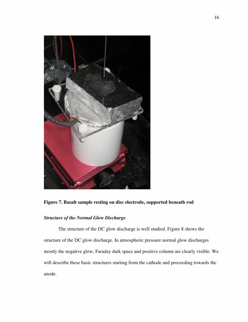
Figure 7. Basalt sample resting on disc electrode, supported beneath rod
Structure of the Normal Glow Discharge
The structure of the DC glow discharge is well studied. Figure 8 shows the
structure of the DC glow discharge. In atmospheric pressure normal glow discharges
mostly the negative glow, Faraday dark space and positive column are clearly visible. We
will describe these basic structures starting from the cathode and proceeding towards the
anode.
Page 25
17
Figure 8. Structure of a DC glow discharge (it is “adapted from J. D. Cobine,
Gaseous Conductors (NY: Dover, 1958), fig. 8.4”)
Cathode. It is an electrical conductor with a secondary emission coefficient which
is very important for the operation of the glow discharge. Secondary electron emissions
occur at the cathode due to ion flux on its surface.
Cathode glow. The next important structure adjacent to the cathode is the cathode
glow. In this region, electrons are energetic enough to excite the neutral atoms they
collide with. The cathode glow has a relatively high ion density. Its axial length depends
upon the surrounding gases and the pressure.
Page 26
18
Faraday dark space. The energy of the electrons are very low in this region. The
electron number density decreases by recombination and diffusion to the walls, the net
space charge is very low, and the axial electric field is small.
Positive glow. The electric field is just large enough to maintain a constant degree
of ionization along its length. In air the color of the positive column plasma is pinkish
blue. As the length of the discharge tube is increased at constant pressure, the length of
the cathode structures remains constant and the length of the positive column increases.
The positive column is a long, uniform glow. Incredibly long positive columns can be
created, for example in the case of neon tubes.
Striations. Moving or standing striations are traveling perturbations in the
electron number density which occurs in partially ionized gases. The moving striations
are propagating bands which appear in positive columns.
Temperature Measurement Using Emission Spectroscopy
The main objective was to use the optical emission spectroscopy to measure the
rotational and vibrational temperature of the glow discharge using the N2 second positive
system (N2 C3 Пu
_B
3 Пg ). This transition is chosen because the N2(C-B) transition can
be seen independent of other transitions for different species and electronic states. A
Boltzmann distribution is assumed with a rotational temperature Trot. The rotational and
translational temperatures Ttran were assumed equal. This is valid considering the short
times of rotational to translational energy transfer. A program called SPECAIR is used to
model spectra of the anode glow, the cathode glow and the positive column. The
temperature measurements were made by computing the RMS error (RMSE) between our
Page 27
19
measurements and the model at 28 wavelength points encompassing the transition in
question. We considered a subset between 360.44 and 381.79 nm from our QE65000
spectrometer data on a single vibrational band centered at 375 nm. Since our
spectrometer is not absolutely calibrated, this window of 21.35 nm will provide better
accuracy since the quantum efficiency is relatively constant in this small range. The
apparatus line broadening was taken into account by convolving the modeled narrow-line
spectra from SPECAIR with the instrument slit function. A spectrum from a calibrated
mercury light source was used to compute the slit function. The search for the best-fit
conditions was computed using a MATLAB script. We find that there are measureable
temperature differences between different parts of the discharge as discussed in the next
section.
Page 28
20
III. RESULTS
Experiment I
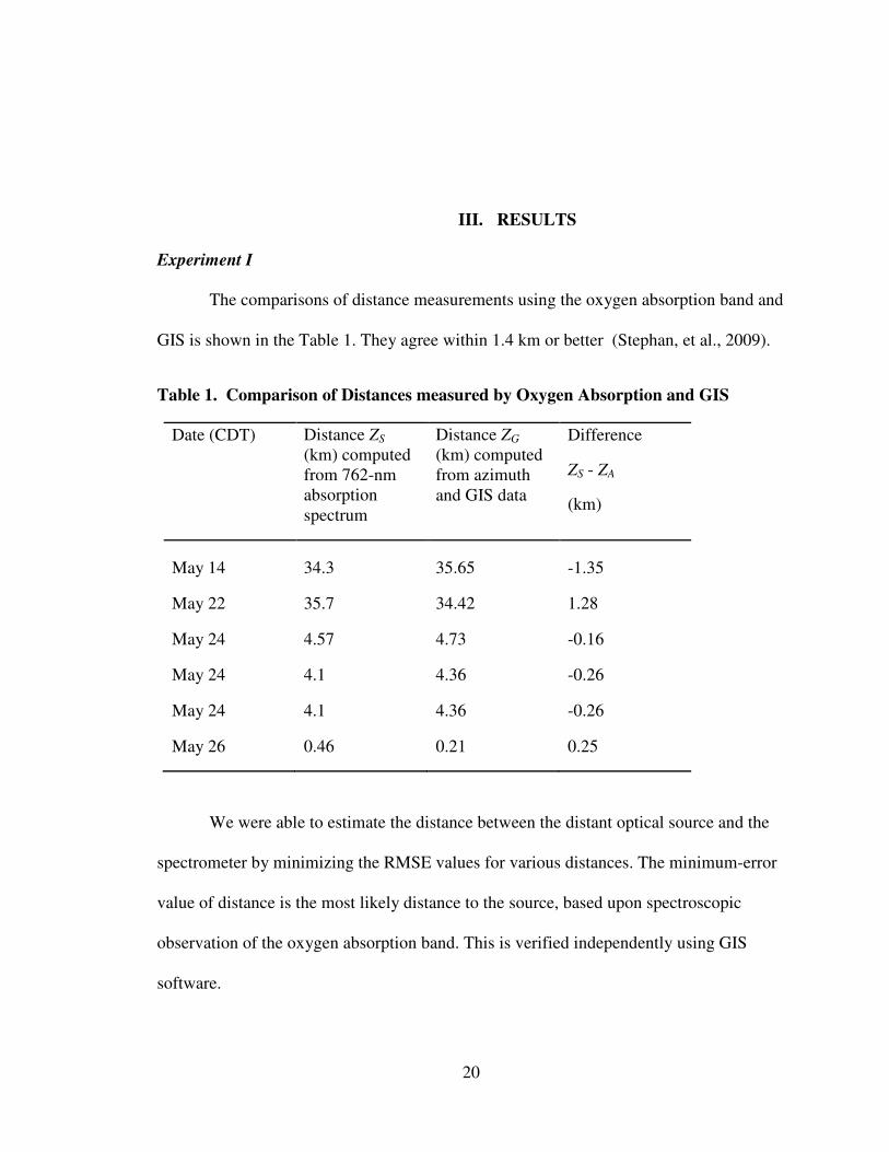
The comparisons of distance measurements using the oxygen absorption band and
GIS is shown in the Table 1. They agree within 1.4 km or better (Stephan, et al., 2009).
Table 1. Comparison of Distances measured by Oxygen Absorption and GIS
Date (CDT) Distance ZS
(km) computed
from 762-nm
absorption
spectrum
Distance ZG
(km) computed
from azimuth
and GIS data
Difference
ZS - ZA
(km)
May 14 34.3 35.65 -1.35
May 22 35.7 34.42 1.28
May 24 4.57 4.73 -0.16
May 24 4.1 4.36 -0.26
May 24 4.1 4.36 -0.26
May 26 0.46 0.21 0.25
We were able to estimate the distance between the distant optical source and the
spectrometer by minimizing the RMSE values for various distances. The minimum-error
value of distance is the most likely distance to the source, based upon spectroscopic
observation of the oxygen absorption band. This is verified independently using GIS
software.
Page 29
21
Experiment II
Photographs of the discharge were taken with a MIRO Phantom 640x480-pixel
high-speed video camera. The photographs taken at speeds as high as 500 fps show that
the discharge is wide and steady. Figure 9 shows a discharge as it appears with a current
of 5.1 mA and a gap length of 30 mm. A small bright-blue cathode spot usually appears
directly on the lower surface of the tungsten rod, but is positioned on the rod so as not to
be visible in Figure 9. Beneath the cathode spot a long pinkish positive column with one
or more stable striations extends downward toward the basalt surface.
The visible width of the positive column, as measured between half-intensity
points on the photo, increases from 800 µm at the widest part of the upper bright region
to about 1000 µm at the widest part below the second striation, where the glow fades into
invisibility. This positive column is not always perfectly stationary. Its motion was
restricted to less than a cm in directions transverse to the electric field, and was
accompanied by minor shifts in the discharge current.
Page 30
22
Figure 9. Photo of 30-mm-long DC atmospheric-pressure normal glow discharge in
air. Current 5.1 mA, voltage 11.4 kV. Note pinkish positive column with two stable
striations, and numerous anode glows on surface of basalt in circle approximately
18 mm in diameter.
A room-light view of the same electrode-rock configuration with no discharge
occurring is shown in Figure 10.
Page 31
23
Figure 10. Room-light view of tungsten electrode and basalt surface
The most interesting aspect of the discharge occurs between the end of the visible
portion of the positive column and the surface of the basalt sample. The blue anode glows
of varying brightness appear over a circular field which was up to 18 mm in diameter or
more, as shown in Figure 9. This is evidence that plasma current from this discharge
widens out at the anode end to cover the 1-2 cm diameter of the illuminated circle.
Shorter gap lengths cause the circle’s diameter to decrease. There was a visible circle at
least a few mm wide for gaps as short as 10 mm.
Page 32
24
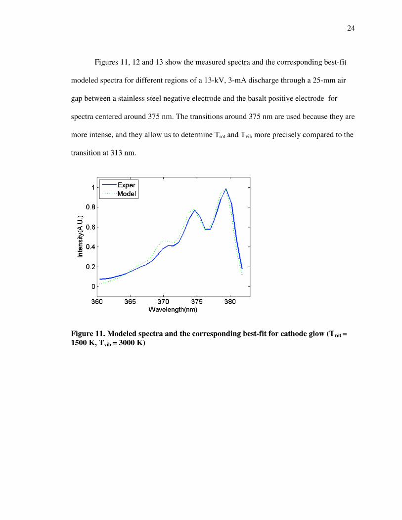
Figures 11, 12 and 13 show the measured spectra and the corresponding best-fit
modeled spectra for different regions of a 13-kV, 3-mA discharge through a 25-mm air
gap between a stainless steel negative electrode and the basalt positive electrode for
spectra centered around 375 nm. The transitions around 375 nm are used because they are
more intense, and they allow us to determine Trot and Tvib more precisely compared to the
transition at 313 nm.
Figure 11. Modeled spectra and the corresponding best-fit for cathode glow (Trot =
1500 K, Tvib = 3000 K)
Page 33
25
Figure 12. Modeled spectra and the corresponding best-fit for positive column (Trot
= 2500 K, Tvib = 2000 K)
Figure 13. Modeled spectra and the corresponding best-fit for anode glow (Trot =
500 K , Tvib = 3000 K )
The experimental spectra were shifted by 0.9 nm towards the short-wavelength
end of the wavelength axis to better match with the modeled spectra. From the simulation
Page 34
26
results shown in p.24 and p.25 above, the best-fit temperatures for the positive column
were Trot = 2500 K, Tvib = 2000 K. For the cathode glow column, Trot = 1500 K, Tvib =
3000 K, and for the anode glow they were Trot = 500 K, Tvib = 3000 K. The accuracy of
the rotational temperature estimated was ± 500 K since we used SPECAIR data with Trot
at increments of 500 K. The rotational temperature in the positive column was the
highest. This is probably due to the fact that most of the plasma voltage drop takes place
in this region and the primary heat-loss mechanisms are limited to convection and
radiation. On the other hand, the anode glow is in close contact with the room-
temperature rock surface, which helps to explain its lower temperature. In the next
section, we will discuss the absolute calibration for our spectroscopic system.
Page 35
27
IV. ABSOLUTE CALIBRATION OF SPECTROSCOPIC SYSTEM
Another important issue is the calibration of the spectroscopic system. The
absolute calibration technique will enable us to measure experimental spectral
irradiance ( )x i
ξ λ (µW cm-2
nm-1
) and spectral radiance ( )x i
L λ (µW cm-2
nm-1
sr-1
). A
QE65000 spectrometer and a re-imager were used to record the spectra of sources. A re-
imager used a 75% reflectivity beam splitter mirror that deflects most of the light to two
planoconvex lenses, concentrating light in 25 mm column down to end of 1 mm diameter
fiber-optic cable. A standard lamp (LS-1-CAL) was used to calibrate the spectrometer for
which spectral irradiance as a function of wavelength is provided by the manufacturer
over the wavelength range from 300 nm to 1050 nm, at 10 nm intervals. Using the 1-mm
fiber optic cable and the QE65000 spectrometer, we obtained a spectrum from the LS-1-
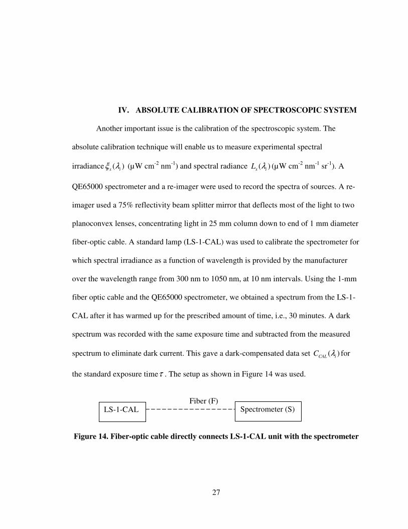
CAL after it has warmed up for the prescribed amount of time, i.e., 30 minutes. A dark
spectrum was recorded with the same exposure time and subtracted from the measured
spectrum to eliminate dark current. This gave a dark-compensated data set ( )CAL i
C λ for
the standard exposure timeτ . The setup as shown in Figure 14 was used.
Figure 14. Fiber-optic cable directly connects LS-1-CAL unit with the spectrometer
LS-1-CAL Spectrometer (S) Fiber (F)
Page 36
28
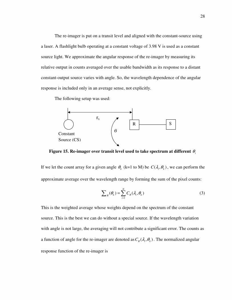
The re-imager is put on a transit level and aligned with the constant-source using
a laser. A flashlight bulb operating at a constant voltage of 3.98 V is used as a constant
source light. We approximate the angular response of the re-imager by measuring its
relative output in counts averaged over the usable bandwidth as its response to a distant
constant-output source varies with angle. So, the wavelength dependence of the angular
response is included only in an average sense, not explicitly.
The following setup was used:
Figure 15. Re-imager over transit level used to take spectrum at different i
θ
If we let the count array for a given angle k
θ (k=1 to M) be ( , )i k
C λ θ , we can perform the
approximate average over the wavelength range by forming the sum of the pixel counts:
1
( ) ( , )N
k R i kRi
Cθ λ θ=
=∑ ∑ (3)
This is the weighted average whose weights depend on the spectrum of the constant
source. This is the best we can do without a special source. If the wavelength variation
with angle is not large, the averaging will not contribute a significant error. The counts as
a function of angle for the re-imager are denoted as ( , )R i k
C λ θ . The normalized angular
response function of the re-imager is
Constant
Source (CS)
rs
R S
Page 37
29
( )
( )max
RR
R
Sθ
θ =∑∑
(4)
The conversion factor i
K is calculated from the fiber cross-sectional area
A (cm2), the calibration data file ( )
CAL iξ λ (µW cm
-2 nm
-1) supplied with the LS-1-CAL
unit, the count array ( )CAL i
C λ resulting from the experiment of Figure 14, and the
maximum value of the count arrayMAX
C .
( )( )
MAXi CAL i
CAL i
CK A
Cξ λ
λ= (µW nm
-1) (5)
Now all count data can be converted to equivalent power data using (6)
**
( )( ) i
i i
MAX
CP K
C
λλ = (µW nm
-1) (6)
The symbol * stands for R, or X (re-imager measurements of experiment on
Figure 15 or the actual experimental data). Assuming that the constant source’s solid
angle as viewed by the re-imager in experiment in Figure 15 is so small that the angular
response function R
S is constant over the solid angle, we can determine the constant
source’s irradiance.
Figure 16. Experimental setup to measure solid angle
Spectrometer Re-imager
Solid Angle ΩX
Experimental
Source CX
rs
R S
Page 38
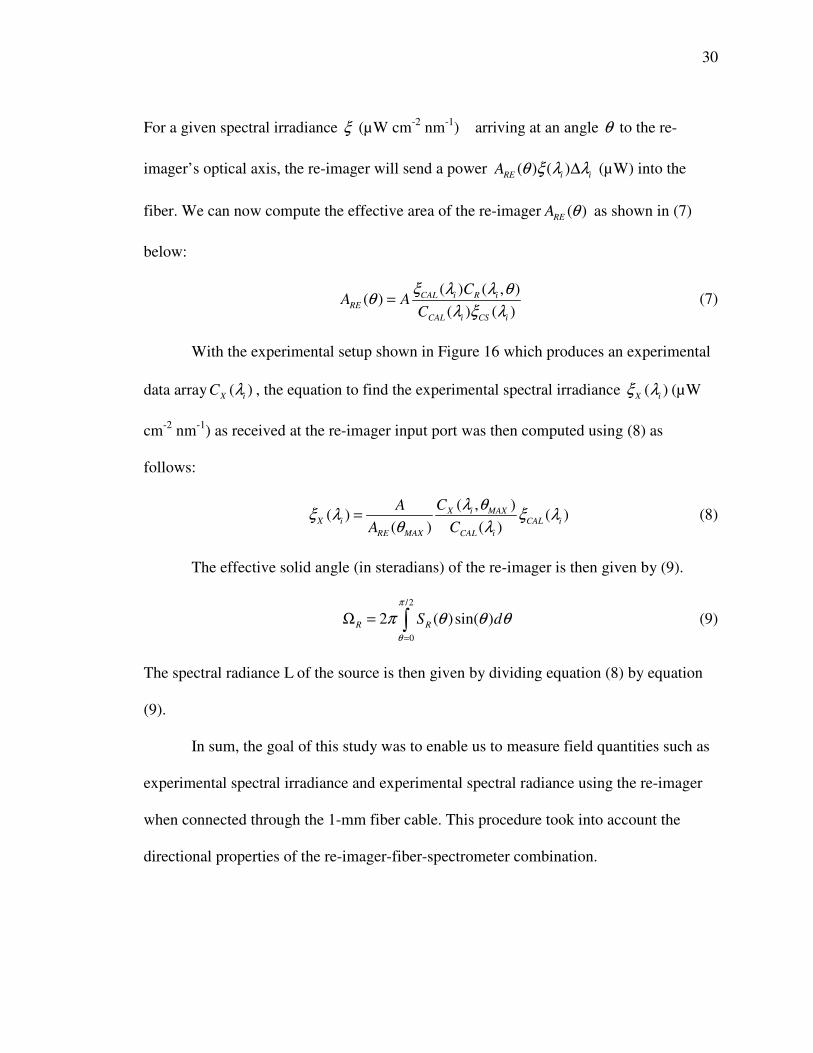
30
For a given spectral irradiance ξ (µW cm-2
nm-1
) arriving at an angle θ to the re-
imager’s optical axis, the re-imager will send a power ( ) ( )RE i i
A θ ξ λ λ∆ (µW) into the
fiber. We can now compute the effective area of the re-imager ( )RE
A θ as shown in (7)
below:
( ) ( , )
( )( ) ( )
CAL i R i
RE
CAL i CS i
CA A
C
ξ λ λ θθ
λ ξ λ= (7)
With the experimental setup shown in Figure 16 which produces an experimental
data array ( )X i
C λ , the equation to find the experimental spectral irradiance ( )X i
ξ λ (µW
cm-2
nm-1
) as received at the re-imager input port was then computed using (8) as
follows:
( , )
( ) ( )( ) ( )
X i MAX
X i CAL i
RE MAX CAL i
CA
A C
λ θξ λ ξ λ
θ λ= (8)
The effective solid angle (in steradians) of the re-imager is then given by (9).
/2
0
2 ( )sin( )R RS d
π
θ
π θ θ θ=
Ω = ∫ (9)
The spectral radiance L of the source is then given by dividing equation (8) by equation
(9).
In sum, the goal of this study was to enable us to measure field quantities such as
experimental spectral irradiance and experimental spectral radiance using the re-imager
when connected through the 1-mm fiber cable. This procedure took into account the
directional properties of the re-imager-fiber-spectrometer combination.
Page 39
31
V. DISCUSSIONS
Plasma spectroscopy which focuses on atomic and molecular emission spectra of
low temperature plasmas or other light sources is a powerful diagnostic tool. With a very
simple experimental set-up it provides a non-invasive diagnostic method. Although
spectra are recorded easily, interpretation of those spectra can be a complex task.
Although we did not see any genuine Marfa lights during our 20-night
observation, we showed that from the analysis of spectral data we can draw unequivocal
conclusions about the origin of all light sources that were bright enough to produce
spectra with an adequate signal-to-noise ratio. We used the Fraunhofer A-band due to
absorption of molecular oxygen to determine the distances of several continuum-
spectrum light sources.
In the second part of the thesis, the atmospheric pressure DC normal glow
discharge is discussed. The DC normal-glow discharge's practical applications make it a
highly sought-after type of plasma, but virtually all applications of this type of plasma
require pressures below atmospheric. We have demonstrated that natural porous rock can
support a large-area DC normal glow discharge up to 18 mm in diameter. This finding is
unprecedented in the literature. We believe that the rock’s pores have a stabilizing and
enlarging effect on the plasma through the air. Temperature measurements, visualization
and parametric studies of the discharge show it to be a normal glow discharge. Emission
spectroscopy and gas temperature measurements using the 2nd positive band of N2
indicate that the discharge forms non-equilibrium plasma. Although we have studied only
Page 40
32
natural basalt extensively, field studies with a portable high-voltage setup show that the
same type of phenomenon can occur with a wide variety of other rocks such as granite.
The essential requirements seem to be only that the rocks must have water content in
them. Finally, absolute calibration of our spectroscopic system could be implemented
based on the mathematical derivations we have presented and this would allow us to
compute experimental spectral irradiance and experimental spectral radiance. Due to lack
of time and a proper calibrated source, results for absolute calibration for the plasmas
could not be completed. All of our spectroscopic analysis was therefore based on relative
intensities.
In sum, this research may have important implications for the scientific study of
various atmospheric phenomena, such as ball lightning and Marfa lights. Besides, there
are many important applications of non-thermal plasmas to the manufacturing of
materials such as in the manufacturing of microelectronics and integrated circuits. Plasma
processing also plays important role in textile processing and biomedical applications.
Page 41
REFERENCES
Abrahamson, J., Bychkov, A. V., & Bychkov, V. L. (2002). Recently Reported Sightings
of Ball Lightning: Observations Collected by Correspondence and Russian and
Ukrainian Sightings. Philosophical Transactions: Mathematical, Physical and
Engineering Sciences, 360(1790), 11-35.
Bunnell, J. (2009). Marfa Lights Research. Retrieved October 27, 2009, from
www.nightorbs.net
Fantz, U. (2006). Basics of plasma spectroscopy. Plasma Sources Science and
Technology, 15(4), S137.
Garamoon, A. A., & El-zeer, D. M. (2009). Atmospheric pressure glow discharge plasma
in air at frequency 50 Hz. Plasma Sources Science and Technology, 18(4),
045006.
Hall, M. (2006). The Truth Is Out There. Retrieved October 27, 2009 from
http://www.texasmonthly.com/preview/2006-06-01/feature2.
Laux, C. O., Spence, T. G., Kruger, C. H., & Zare, R. N. (2003). Optical diagnostics of
atmospheric pressure air plasmas. Plasma Sources Science and Technology,
12(2), 125-138.
Pierluissi, J. H., & Tsai, C.-M. (1986). Molecular transmittance band model for oxygen in
the visible. Appl. Opt., 25(15), 2458-2460.
Staack, D., Farouk, B., Gutsol, A., & Fridman, A. (2005). Characterization of a dc
atmospheric pressure normal glow discharge. Plasma Sources Science and
Technology, 14(4), 700-711.
Stephan, K. D., Ghimire, S., Stapleton, W. A., & Bunnell, J. (2009). Spectroscopy
applied to observations of terrestrial light sources of uncertain origin. American
Journal of Physics, 77(8), 697-703.
Stolyarov, A., Klenzig, J., Roddy, P., & Heelis, R. A. (2005). An experimental analysis
of the Marfa lights. Retrieved March 3,2010 from
www.spsnational.org/wormhole/utd_sps_report.pdf.
Wark, D. Q., & Mercer, D. M. (1965). Absorption in the Atmosphere by the Oxygen 'A'
Band. Appl. Opt., 4(7), 839-845.
Page 42
VITA
Sagar Ghimire was born in Morang district of Nepal on January 9, 1979. He is the
son of Dev Kumar Sharma and Shanta Ghimire. After completing his schooling from
Hermann Gmeiner School Sanothimi, Bhaktapur, Nepal in 1994 he entered St. Xavier’s
Campus, Kathmandu, Nepal and completed his Intermediate in Science (I.Sc.) in 1996.
He entered Tribhuvan University, Institute of Engineering in 1996 and completed his
Bachelor’s Degree in Electronics Engineering and Master’s in Information and
Communication Engineering in the years 2001 and 2005 respectively.
He was working as a Telecom Engineer in Nepal Telecom before he entered the
Graduate College of Texas State University-San Marcos in January 2008. During the
following years he served as a Graduate Instructional Assistant in the Department of
Engineering Technology and Ingram School of Engineering for Circuits and Devices,
Digital Electronics, Industrial Electronics, Fields and Waves and Microelectronics
Manufacturing labs.
Email: [email protected]
This thesis was typed by Sagar Ghimire.