NTIA REPORT 80-38 SPECTRUM RESOURCE ASSESSMENT IN THE 2.7 TO 2.9 GHz BAND PHASE II: LSR DEPLOYMENT IN THE LOS ANGELES AND SAN FRANCISCO AREAS (Report No.3) ROBERT L. HINKLE u.s. DEPARTMENT OF COMMERCE Philip M. Klutznlck, Secretary Henry· Geller, Assistant Secetary for Communications and Information APRIL 1980
Transcript
NTIA REPORT 80-38
SPECTRUM RESOURCEASSESSMENT IN THE
2.7 TO 2.9 GHz BANDPHASE II: LSR DEPLOYMENT
IN THE LOS ANGELES ANDSAN FRANCISCO AREAS
(Report No.3)
ROBERT L. HINKLE
u.s. DEPARTMENT OF COMMERCEPhilip M. Klutznlck, Secretary
Henry· Geller, Assistant Secetaryfor Communications and Information
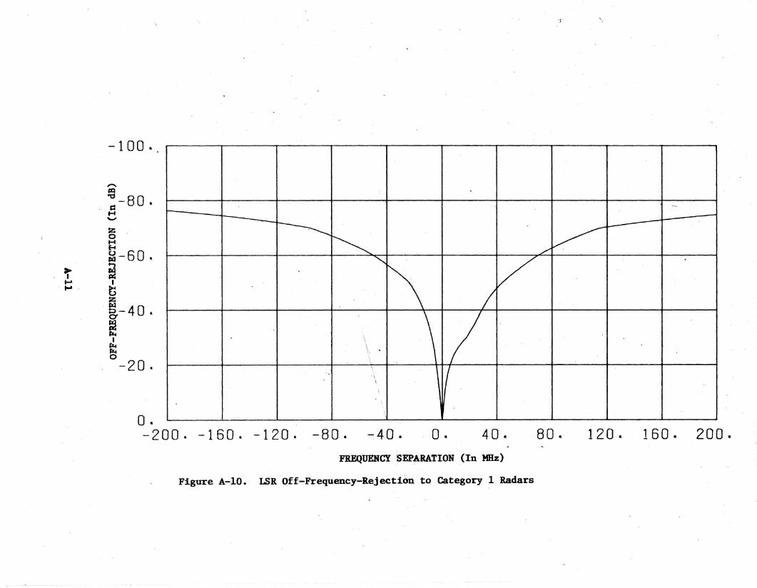
A-10 LSR Off..Frequency-Rejection to Category Radars.
A-11 LSR Off-Fr'equency-Rejection to Category 2 Radars.
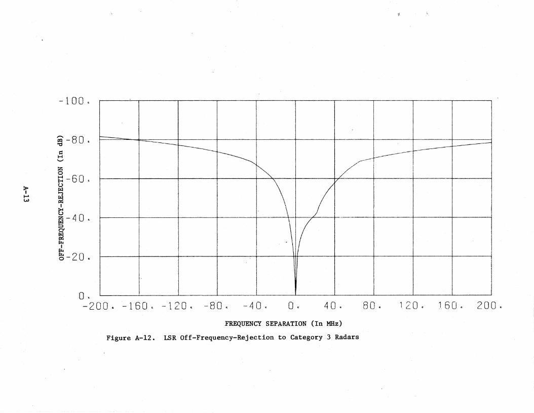
A-12 LSR Off-Frequency..Rejection to Category 3 Radars.
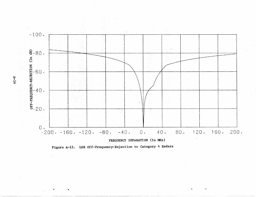
A.... 13 LSR Off-Frequency-Rejection to Category 4 Radars.
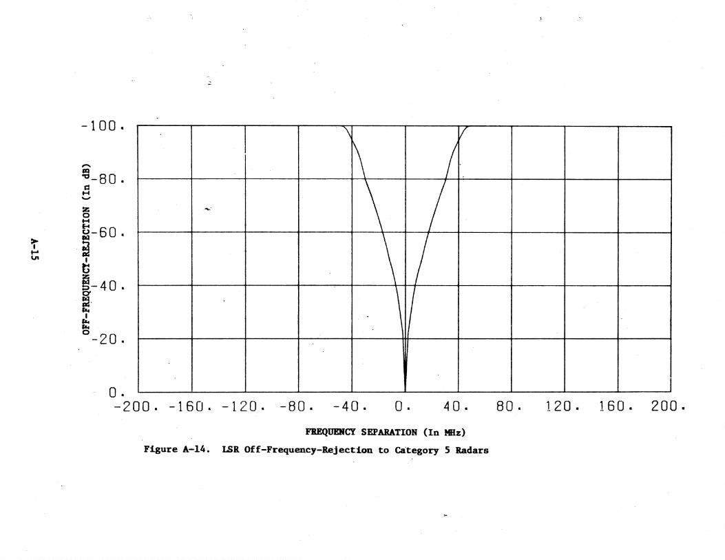
A-14 LSR Off-Frequency-Reject,!on to Category 5 Radars.
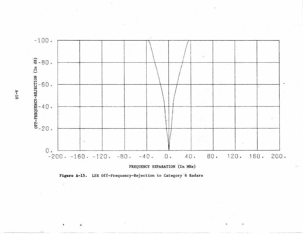
,A-15 LSR Off-Frequency~Rejectlon to Category 6 Radars.
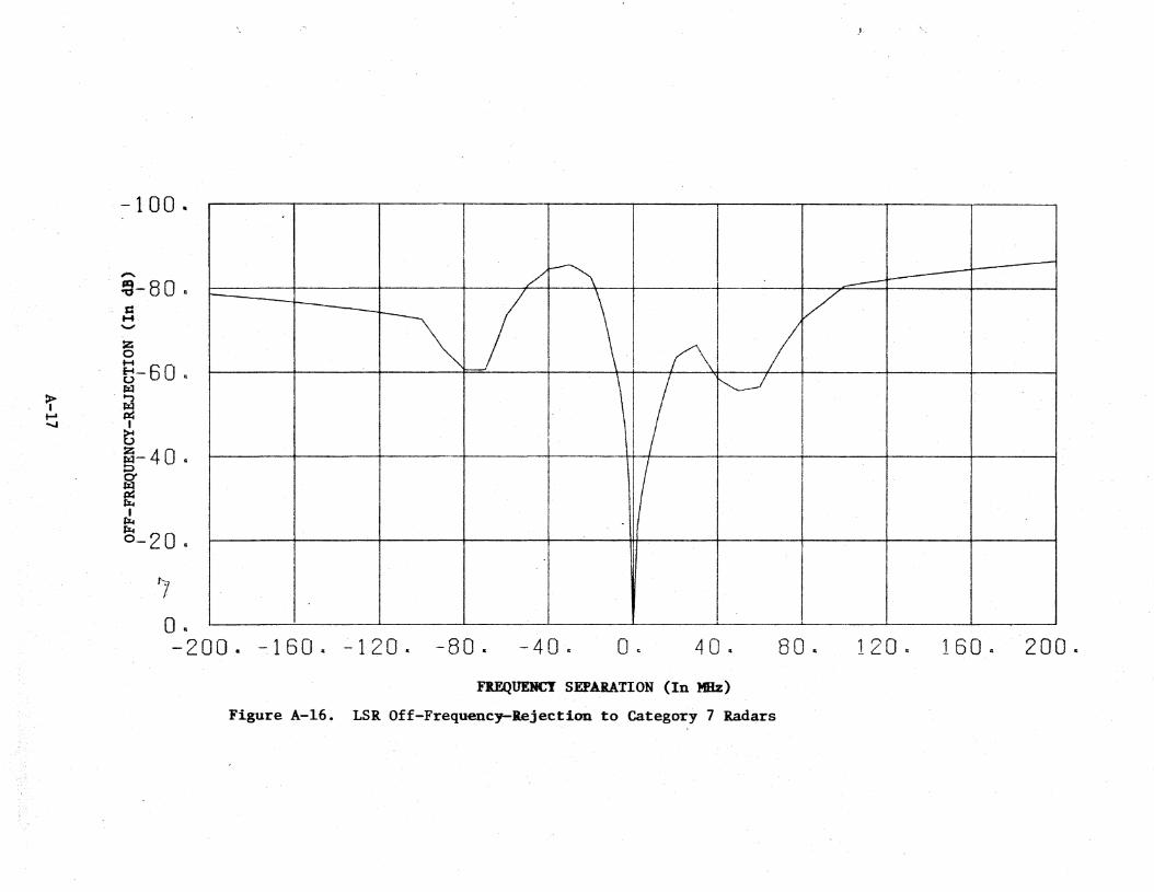
A-16 LSR °ff-Frequency..Rejection to Category 7 Radars.
1-17 LSi Off....Frequency..Rejection to LSR Radars
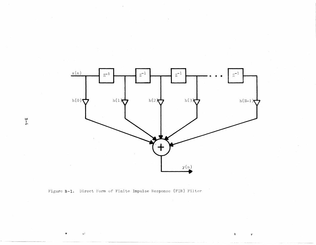
B-1 Direct Form of Finite Impulse Response (FIR) Filter .
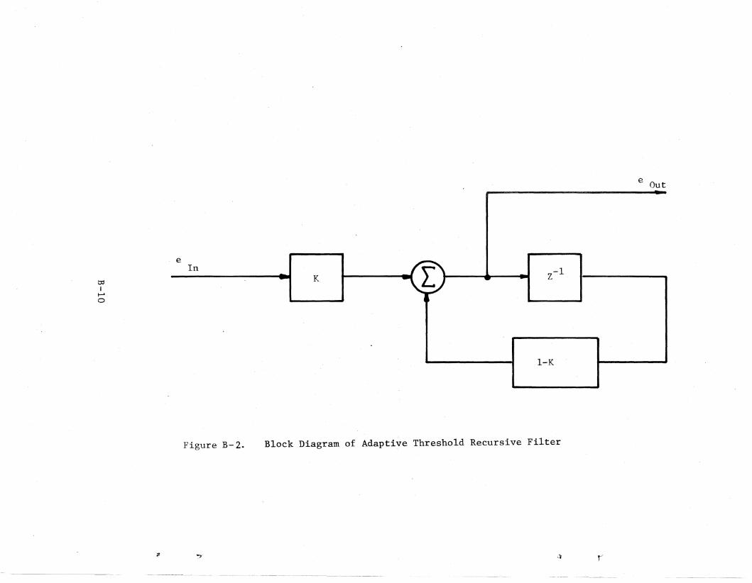
B-2 Block Diagram of Adaptive Threshold Recursive Filter.
LIST OF TABLES
IABLE
Frequency As'signments in 2.7 to 2.9 GHz Band.
A-8
A-9
A-11,
A-12
A-13
A-14
A-15
A.. 16
A-11
A-18
B-4
B.... 10
1..3
2-1 ' Available Operating Frequencies and Percentage of BandAvailable for LSR Operation in the Los Angeles Area • 2-3
2-2 Available Operating Frequenoies and Percentage of BandAvailable for LSR Operation in the San Franoisco Area
3.... 1 LSR System Characteristics.
Propagation Los_s Below Free Space Due to Various UrbanEnvironments. . .. .,. . • • • . .. . . .
5-1 Location of.2.7-2.9 GHz Radars in Los Angeles Area.
5·2 Characteristics of 2.7-2.9 GHz Radars in Los Angel~s Area .
5-3 Propos~d Locations of LSRs in Los Angeles Area .• ' .
5....4 Imperial LSR Site
5-5 Brown LSR Site ..
vi
2..5
3-2
4....8
5-2
5-5
5-8
5-10
5-12
5-6
5-7
5-8
5-9,..,
6-1
6-2
6-3
6-4
6-5
6-6
6-7
6-8
6-9
6-10
A-1
B-1
B-2.
B-3
Gillespie LSR Site.
El Monte LSR site
Palmdale LSR Site .
Santa Maria LSR Site.
Location of 2.7-2.9 GHz Radars in San Francisco Area •.
Characteristics of 2.7-2.9 GHz Radars in San Francisco Area
Proposed Locations of LSRs in San Francisco Area.
Merced LSR Site . .
Modesto LSR Site.
Livermore LSR Site ..
StocktonLSR Site .
Concord LSR Site.
Napa County LSR Site.
Santa Rosa LSR Site . . .
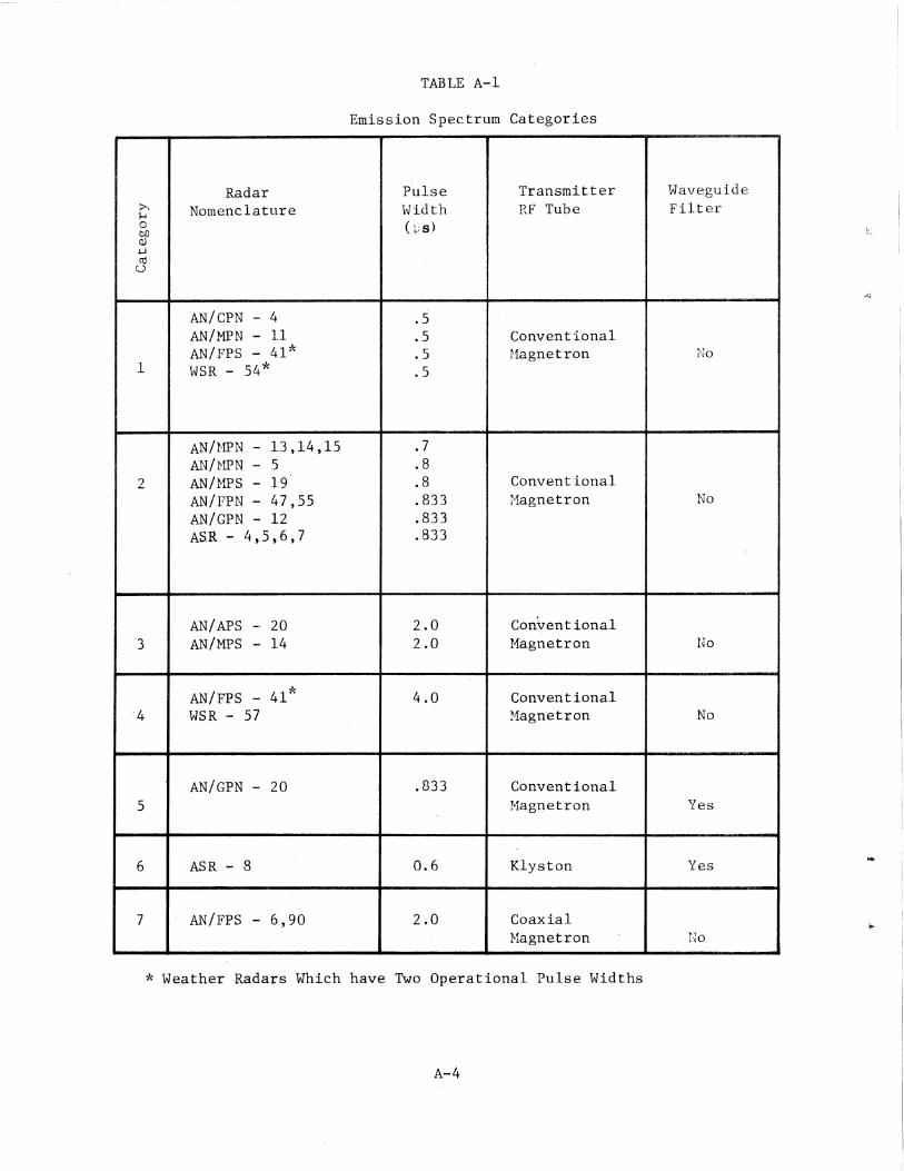
Emission Spectrum Categories.
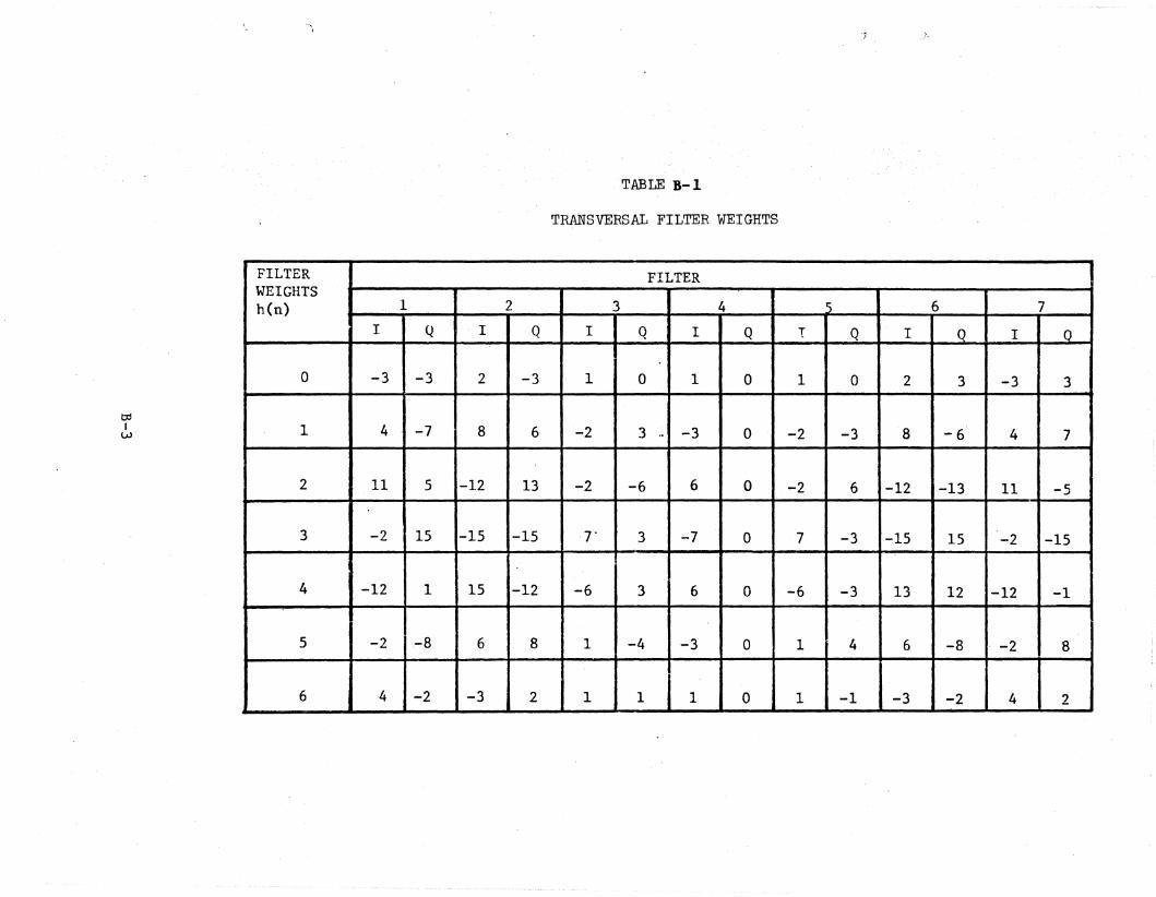
Transversal Filter Weights...
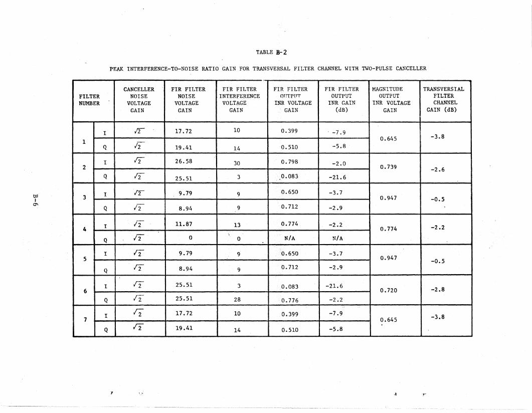
Peak Interference-to-Noise Ratio Gain for Transversal FilterChannel with Two-Pulse Canceller. . . .. . . . . . . . .
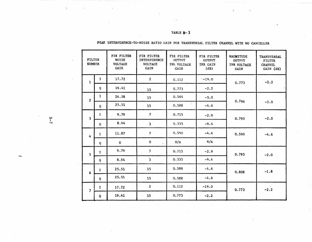
Peak Interference-to-Noise Ratio Gain for Transversal FilterChannel with No Canceller . . . . . . . . . . . . . .
5-13
5-14
5-16
5-17
6-2
6-4
6-6
6-8
6-10
6-11
6-12
6-13
6-15
6-16
A-4
B-3
B-6
B-7
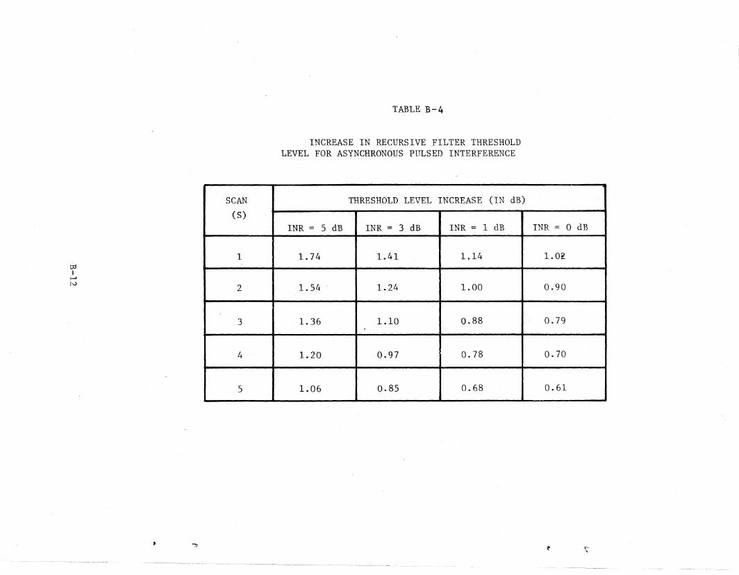
B-4 Increase in Recursive Filter Threshold Level for AsynchronousPulsed Interference . . .. B-12
B-5 Peak INR Performance Criteria for MTD-II Radar. B-15
vii
ABSTRACT
,The National Teleo~mmunloat1:.nsand. Information Adm1n1stra,t1on (NTIA) in 'theDepartment of Commerce undertook a detailed program to investigate thefeaaibility of deploying the Limited Surveillance Radars (LSR) in the 2 •7-2 .9 Q.Hzband in the Los Angeles and SanFranoiscoarea$ • The LSR 1s " Federal AviationAdministration (FAA) air traffio <control radar planned to'r use at generalaV1a'tionairports with h1ghtraf,fio density that do not qualify for the longerrang.e Air,port Surveillance Radaria (ASH). This investigation was .thethird in aserl ies of t'asks undertaken byNTIA as part ofaspect,rumresoliroe assessmeht ,ofthe, ,2 .1-2 •9GHz band. The overall objective of thespeotrum resouroeaasesementwas to assess the degree of oo.ngestion in the band in deslgnatedareas in theU'nlt:ed States,and to promote more effeotive utilization of the b·.nd.
The investigation showed ii,that the 2.7-2.9 GHz band 1s oong,ested in both theLos Angeles and San Franciaco areas. Major factors oontr1butil\8to ,oongest:1onare the Military height-finding radars and the 00ou,r:ance ofducting(superrefraotion) propagationcondit1ons. However, the LSR radarsoan beacoommodated in the present environment at the proposed sites lntheseareas, butit was' necesaary to oo,nduot a detailed frequenoya881gnment1nv,est1aation. Dueto the high degree of.oongestion in these areas, it may be necessary, in order toaccommodate all the .proposedLSR deployments, to retrofit arew existing radarsin the env1rorment with waveguide filters or reoeiver signal processingtechniques to suppress asynchronous pulsed interference.
Limited Surveillanoe RadarDeployment
Frequency AssignmentEleotr.omagne't10 Compatibilit,Y
viii
SECTION 1
INTRODUCTION
BACKGROUND
During the period of August 1971 through' April 1973, the InterdepartmentRadio Advisory Committee (IRAC) had under study the accommodation of Departmentof Defense (DoD), Federal Aviation Administration (FAA), and Department ofCommerce (DoC) radar operations in the band 2.7-2.9 GHz~ A series of meetingswere held between the agencies (Summary Minutes of the First (October 1972) andSecond (December 1972) OTP Meetings) to determine if new FAA air - traffic controlradars could be accommodated in this' band without degrading their performance,and what impact these radars would have on the performance of existing radars inthe band. An initial assessment of the problem (Maiuzzo, 1972) determined thatthe addition of new radars to the band could create.a potential problem. Toresolve the immediate problem of accommoda.ting the new FAA Air Traffic ControlRadars, the following actions were taken:
a. The band 3.5-3.7 GHz was reallocated by footnote to provide forco-equal primary Government use by both the AeronauticalRadionavigatidn and Radiolocation Services. The footnote reads asfollows:
G110 - Government ground-based stations in theaeronautical radionavigation service may be authorizedbetween 3.5-3.7 GHz where accommodation in the 2.7-2.9 GHzband is not technically and/or economically feasible.
Agencies were requested to cooperate ' to the maximum extentpracticable to ensure on an area-by-,area, case-by-case basis that theband 2.7-2.9GHz is employed effectively.
b. The Spectrum Planning subcommittee was tasked to develop a long-rangeplan for fixed radars with emphasis on the 2.7-2.9 GHz and3.5-3.7 GHz bands. The SPS plan (SPS Ad Hoc Committee, 1974) wascompleted and approved by the IRAC.
The Office of Telecommunications Policy (OTP)' subsequently tasked the Officeof Telecommunications (OT)' to perform a spectrum resource assessment of the2.7-2.9 GHz band. The intent of this assessment was to provide a quantitativeunderstanding of potential problems in the band of concern as well as to identifyoptions available to spectrum managers for dealing with these problems. One ofthe primary reasons for initiating the assessment· was to ensure identification ofproblems during the early phases of design and planning rather thanafter-the-fact, i.e., after a system has been designed and hardware fabricated.By -making these band assessments early, necessary actions. can be taken to assurethat appropriate communication channels are established petween agencies whosesystems are in potential conflict. This will enhance the early identification ofsolutions which are mutually satisfactory to all parties involved.
'OTP and OT have been reorganized into the National Telecommunications andInformation Administration (NTIA) within the Department of Commerce.
1-1
A, mult1phaseprogram' to the: solution of th,e 2.1-2.9 GHz' Speotrum Re,souroeAsseSiSJIen't task waa<'undertakenby, NTIA •
Phase I - The t'irs,t phase involved .the identification of systems existing inand planned for the band in question,.determination of availableteohnioal andope'rational data for eaoh systera, identifioation of the potential inter'aotion~
between systems, and the se'nerat:ion of a plan t'hat leads to an overall a,sses,sme~t
of the band's potential oongestion. A Phase I report (Hinkle and Mayher, 1975)for the. 2.7-2.9 GHz Spectrum Resource Assessment was oompleted.
Pqas!e . ~l - The, second. phase encompassed several tasks:
1. A detailed measurement and model validation program in theLos Angeles and San Fran:cisooareas. The objeotive of t.nistask was to validate mode-ls and prooedures used to predtotradar·to.radar interferenoe, and assess the oapability.ofpredioting bandconsestion. This task was oompleted andthe findings given 1n a report by Hinkle, Pratt, andMatheson (1976).
2. Inv8st11at1on of the 81analprooe.8.1ns proper-tie·. ofprimary radars.1nthe 2.7-2.9'GHz band and the AutomatedRadar Terminal System (ARTS-IlIA) to assess the capabilityof theRada~stosuppressasynohronous interference and thetracle-offs insuppresl1ns; asynohronous 8.110a18. This taskwasoompletedand the f1nd1ngsgiven in a report by Hinkle,Pratt and Levy (1979).
3. Investigation of the feasibility of aooommodat1ns newradar systems 1n the 2.7 to 2.9 GHz ,band in eightdesignated oongested areas (Los Angeles, San Francisoo,New York, Philadelphia, Atlanta, Miami, Chioago, andDallas).
4 • Dev'elopment of engineering and management aids to assistthe frequenoy manager in determ.ining if new radars oan beaooOllDlodated 1n the 2.7-2.9 GHz band, and a methodoloSY forassessing how effioiently the band 1s being utilized.
This report is the third Phase' II report in a series of reports related tothe SpeotrumResouroe Assessment of the 2.7-2.9 GBz band. The report containe an
-invest1sat1onotthefeasib11i;y of aooommodat1ns theL1m1ted SurveillanoeRadar(LSR) in the LOI 'Anselesand S.n Franoisooareas in the 2.7...2.9 GHz bands withoutdegrading the performanoeo! existing radars, Qr the LSBradara.
ENVIRQNtJIHI
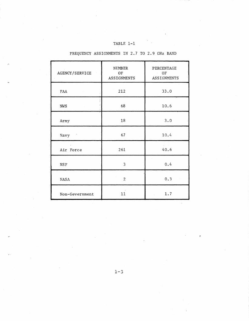
The Government Master File (GMF) ourrently lists 642 Creque.ncy assisnments 1nthe 2.7 to 2.9 qHz band. Major systems in the band inolude theF!A AirportSurveillance Radars (!SRs), DoD Ground Control App.roach (GCA) radars, and DoCNational Weather Service' (NWS) radars. TABLE 1-1 lists the number of frequenoy
1-2
TABLE 1-1
FREQUENCY ASSIGNMENTS IN 2.7 TO 2.9 GHz BAND
NUMBER PERCENTAGEAGENCY/SERVICE OF OF
ASSIGNMENTS ASSIGNMENTS
FAA 212 33.0
NWS 68 10.6
Army 18 3.0
Navy 67 10.4
Air Force 261 40.6
NSF 3 0.4
NASA 2 0.3
Non-Gevernment 11 1.7
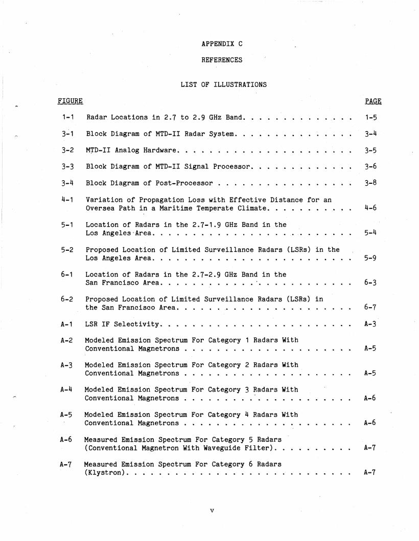
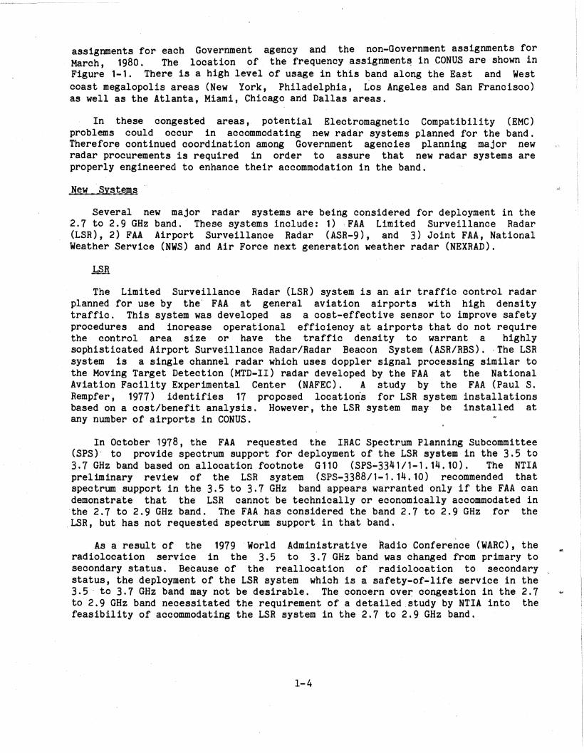
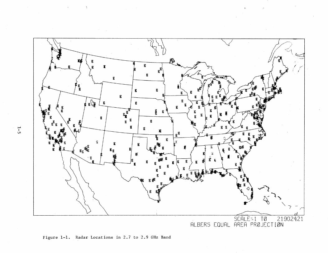
assignments for- each Government agency and the non-Government assignments forMarch, 1980. The location of the frequency assigriment~ in CONUS are shown inFigure 1-1. There is a high level of usage in this ~and along the East and Westcoast megalopolis areas (New York, Philadelphia, Los Angeles ,and San Francisco)as well as the Atlanta, Miami, Chicago and Dallas areas.
In these congested areas, potential Electromagnetic Compatibility (EMC)problems could occur in accommodating new radar systems planned for the band.Therefor~ continued coordination among Government agencies planning major newradar procurements is required in order to assure that new radar systems areproperly engineered to enhance their accommodation in the band.
New Sy~t_e.Ills
Several new major radar systems are being considered for deployment in the2.7 to 2.9 GHz band. These systems include: 1) FAA Limited Surveillance Radar(LSR), 2) FAA Airport Surveillance Radar (ASR-9), and 3) Joint FAA, NationalWeather Service (NWS) and Air Force next generat!on weather radar (NEXRAD).
The Limited Surveillance Radar (LSR) system is an air traffic control radarplanned for use by the' FAA at general aviation airports with high densitytraffic. This system was developed as a cost-effective sensor to improve safetyprocedures and increase operational efficiency at airports that do not requirethe control area size or have the traffic density to warrant a highlysophisticated Airport Surveillance Radar/Radar Beacon System (ASR/RBS). -The LSRsystem is a single channel radar which uses doppler signal processing similar tothe Moving Target Detection (MTD-II) radar developed by the FAA at the NationalAviation Facility Experimental Center (NAFEC). A study by the FAA (Paul S.Rempfer, 1977) identifies 17 proposed locations for LSR system installationsbased on a cost/benefit analysis. However, the LSR system may be installed atany number of airports in CONUS.
In October 1978,the FAA requested the IRAC Spe·ctrum Planning Subcommittee(SPS)- to provide spectrum support for deployment of the LSR system in the 3.5 to3.7 GHz band based on allocation footnote Gll0 (SPS-3341/1-1.14.10). The NTlApreliminary review of the LSR system (SPS-3388/1-1.14.10) recommended thatspectrum support in the 3.5 to 3.7 GHz band appears warranted only if the FAA candemonstr~te that the LSR cannot" be technically or economically accommodated in-the 2.7 to 2.9 GHz band. The FAA has considered the band 2.7 to 2.9 GHz for the.LSR, but has not requested spectrum support in that band.
As a result of the 1979 World Administratiye ~adio Confere~ce (WARC), theradiolocation service in the 3.5 to 3.7 GHz band was changed from primary tosecondary status. Because of the reallocation of radiolocation to secondarystatus, the deployment of the LSR system which is a safety-or-life service in the3.5 . to 3.7 GHzband may not be desirable. The concern ove~ congestion in the 2.7 ~
to 2.9 GHz band necessitated the requirement of a detailed.study by NTlA into thefeasibility of accommodating the LSR system in the 2.7 to 2.9 GHz band.
1-4
~I
Ln
,g
g
g
ig
/
/' ,...-/
[ "
g '~Kg
Ie g g
g g
glJg g
g ~~
J'\ ~"~ "'I
SCRLE~l T0 21902421RLBERS EQURL RRER PR0JECTI0N
Figure 1-1. Radar Locations in 2.7 to 2.9 GHz Band
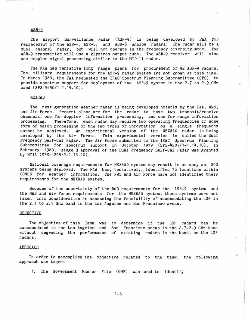
The Airport Surveillance Radar (ASH-g) is being develop\ed by FAA forreplacement o,r the ASR-4, ASR-5, and ASB-6 analog r'adars. The radar will be adual channel radar, but will not operate in the frequency diversity mode. TheASB-9 transmitter will use a klystron output tube. The ASR-9 receiver will alsouse d.oppler signal processing similar to the MTD-II radar.
The FAA has tentative long range plans for procureme'nt of 92 A311-9 radars.The military requirem'ents for the ASR-9 radar system are not known at this time.In March 1980, the FAA requested tthe IRAC Spectrum Planning Subcommittee (SPS) toprovide spectrum support for deployment of the ASR-9 system in th.e2. 7 to 2. 9 .GHzband (SP3-4440/1-1.14.10).
,NEXRAD
The next generation weather radar is being developed jointly by the FAA, NWS,and Air Force. Present plans are for the radar to have two transmit/receivechannels; one for doppler information processing, and one for range informationprocessing. Therefore, e'&ch radar may require two operating frequencies if someform of batch processing of the two types of information on a single frequencycannot be achieved. An experimental version of the NEXRAD radar is beingdeveloped by the Air Force. This experimental version is called the DualFrequency Self-Cal Ra~ar. The Air Force submitted to the IRAC Spectrum PlanningSubcommittee for spectrum support in October 1979 (SPS-4203/1-1.14.10). InFebruary 1980, stage 3 approval of the Dual Frequency Self-Cal Radar was grantedby NTIA (SPS~4294/2-1.14.10).
National coverage requirements for NEXRAD system may result in as many as 200systems being deployed. The FAA has, tentatively" identified 76 locations withinCONUS for weather information. The NWS and Air Force have not identified theirrequirements for the NEXRAD system.
Because of the uncertainty of the DoD requirements for the ASH-9 system andthe NWS and Air Force requirements for the NEXRAD system, these systems were notta.ken into consideration in assessing the feasibility of accommodating the LSR inthe 2.7 to 2.9 GHz band in the Los Angeles and San Francisco areas.
OBJECTIVE,
The objective of this Task wasaccommodated in the Los Angeles andwithout degrading the performanceradars.
APPRQACH
to determine if the LSR radars can beSan Francisco areas in the 2.7-2.9 GHzbandof existing radars in the ba.nd, or the LSR
In order to accompl.ish the objective related to the. task, the followingapproach was taken:
1. The Government Master File (Gi"1F) was used to identi·fy
1-6
existing radars and their operating frequencies in'the 2.72.9 GHz band in the Los Angeles and San Francisco areas.The GMF information was then verified with the FAA and DoDWestern Region frequency coordinators.
2. Use information provided by FAA in 1d,entifying proposedsite locations for LSR radar system deployments in theLos Angeles and San Francisco areas.
3. Establish an appropriate Interference-to-Noise Ratio (INR)performance criterion for the LSR system.
4. Assess the feasibility of accommodating the LSR radars inthe 2.7-2.9 GHz band by using the procedure outlined inthe report by Hinkle, Pratt and Matheson (1976), andtaking into consideration propagation phenomena related tobuilding attenuation and ducting.
1-7
SECTION 2
CONCLUSIONS AND_RECOMMENDATIONS
INTRODUCTION
This section contains a summary of the conclusions and recommendationsresulting from an investigation into the feasibility of accommodating the LimitedSurveillance Radars (LSRs) in the 2.7 to 2.9 GHz band in the Los Angeles and SanFrancisco areas. The investigation did not take into consideration thedeployment of the ASH 9 and NEXRAD radar systems planned for the band because ofunknown requirements for these systems.
The conclusions and recommendations are based on the LSR systemcharacteristics and performance criterion given in Section 3. Finalspecifications for procurement of the LSR system have not been determined, andany changes to the LSR system specifications as given in Section 3 maynecessitate changes in the findings of this investigation. The procedure usedfor determining possible operating frequencies at proposed LSR sites i,s discussedin Section 4.
CONCLUSIONS
A detailed frequency assignment procedure was used to determine thefeasibility of accommodating the LSR system at six proposed sites in the LosAngeles area and eight proposed sites in the San Francisco area. This led to thefollowing conclusions, which are discussed in detail in Section 5 for the LosAngeles area and Section 6 for the San Francisco area.
General
General conclusions resulting from the LSR deployment investigation are:
1. The 2'.7 to 2.9 GHz band is congested in both the Los Angeles andSan Francisco areas~ Howeyer, a detailed frequency assignmentinvestigation indicates that the Limited Surveillance Radars(LSRs) can be accommodated at the proposed sites in these areas.
2. Due to the high degree of congestion in these areas, it may benecessary, in order to accommodate all the proposed LSRdeployments, to retrofit a few existing radars in the environmentwith waveguide filters or receiver signal processing techniquesto suppress asynchronous pulsed interference. However, the costof retrofitting existing radar systems to eliminate interferencemust be weighed against the problems created by the interference,and the scheduled replacement of the existing radar systems.
3. Previ~us investigations (Hinkle, Pratt and Levy, ,1979) have shownthat existing digital radar receivers have the signal processingcircuitry to suppress asynchronous pulsed interference. At thistime, tests have not been conducted to determine if the analogradar receivers have the signal processing circuitry to suppress
2-1
asynchronous pulsed interference.
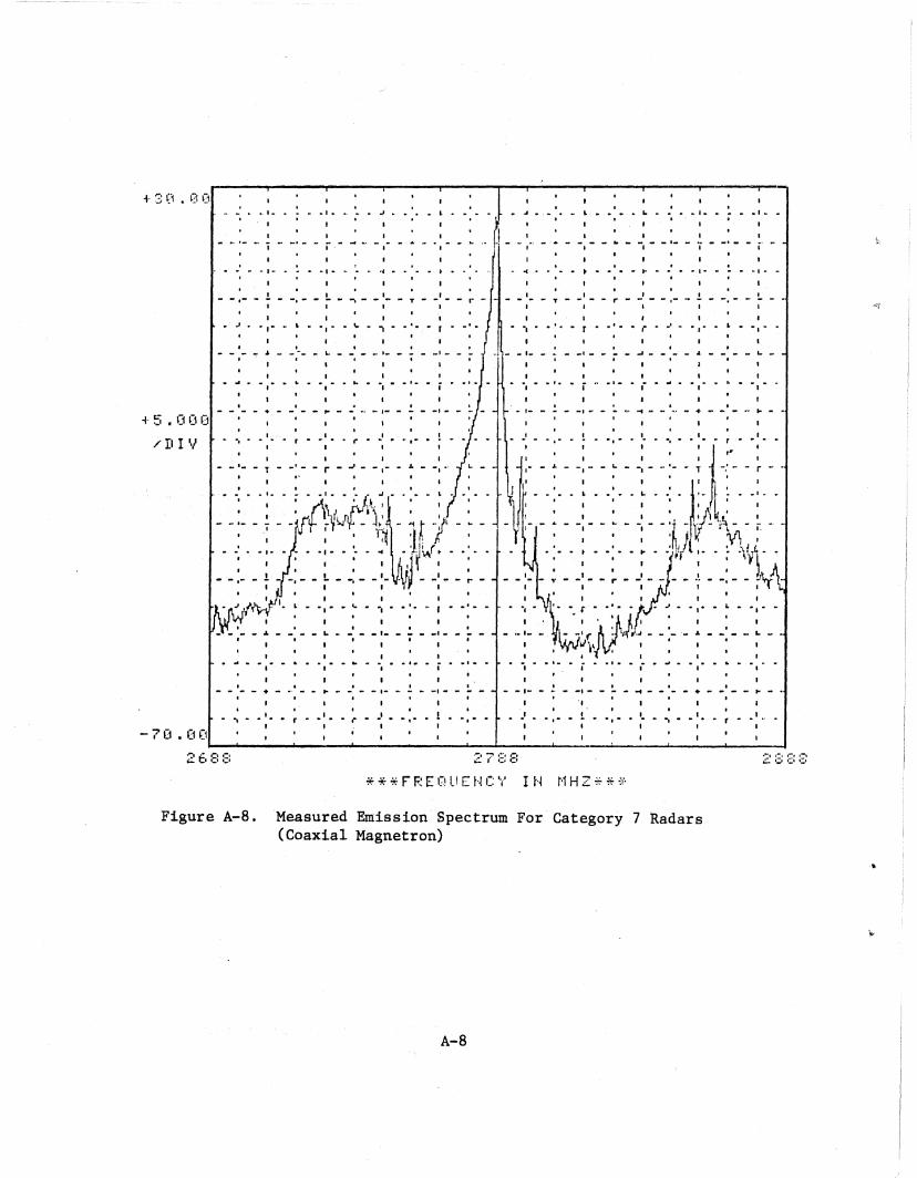
4. 'The height-finding radars are a major contributor to congestionin the band. Measurements made with the Radio SpectrumMeasurement System (RSMS) van show that the coaxial magnetronoutput tube used in the height-finding radars have spurious modeswhich produce high level emissions in, the band thus denying theuse of a large percentage of the band to other potential users.Other height-finding radar characteristics which contribute tocongestion are their site location (generally' on top of hills andmountains), and their relatively high transmitter power andantenna g.ain.
5. The occurrence of ducting (superrefraction) propagationconditions along the coast of Southern California alsocontributes to congestion in the Los Angeles and San Franciscoareas. The ducting propagation phenomenon occurs approximately 50percent of the time during the summer, and must be taken intoaccount in determining frequency assignments which will result incompatible operations.
6. Because of the degree of congestion in the 2.7-2.9 GHz band insome areas, new radar procurements for the Aeronautical Radionavigation.service as well as the Meteorological Aids servicewill have to contend with asynchronous pulsed interference inperforming their operational requirements. Emphasis must beplaced upon the design standards of new equipment requiring l'owtransmitter emission spectrum sideband levels to minimizeadjacent channel interference, and receiver signal processingcircuitry to suppress asynchronous pulsed interference. The useof these spectrum conservation techniques would more readilypermit the accommodation of new radar deployments in the band.
7. Reallocation of the radiolocatiori service in the 3500-3700 MHzband from primary to secondary status by the 1979 WARe requiresthat further consideration be given to the desirability ofdeploying the LSR system in the 3500-3700 MHz band.
8., An analytical investiga.tion of the developmental LSR system(MTD-II) showed that an Interference-to-Noise Ratio (INR)criterion of 5 dB or less would preclude asynchronous pulsedinterference from causins false reports and raising the adaptivethreshold by more than one dB.
LQ§ Ang~les Are~
- The following is a summary of conclusions resulting from an investigationinto the feasibility of deploying Limited Surveillance Radars (LSRs) at sixproposed sites.in the Los Angeles area:
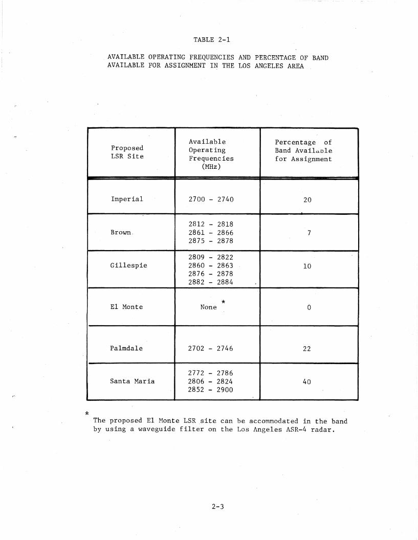
1. Table 2-1 shows the available operating frequencies and
2-2
TABLE 2-1
AVAILABLE OPERATING FREQUENCIES AND PERCENTAGE OF BANDAVAILABLE FOR ASSIGNMENT IN THE LOS ANGELES AREA
Available Percentage ofProposed Operating Band Avai1a.b1eLSR Site Frequencies for Assignment
(MHz)
Imperial 2700 - 2740 20
2812 - 2818Brown. 2861 ~ 2866 7
2875 - 2878
2809 - 2822Gillespie 2860 - 2863 10
2876 - 28782882 - 2884
*El Monte None 0
Palmdale 2702 - 2746 22
2772 - 2786Santa Maria 2806 - 2824 40
2852 - 2900
*The proposed El Monte LSR ,site can be accommodated in the bandby using a waveguide filter on the Los Angeles ASR-4 radar.
2-3
percentage of the 2.7 to 2.9 GHz hand usable 'for frequencyassignment for each ot the proposed LSR, sites. LSRs can bedeployed at five of the six proposed" LSR sites withoutperformance degradation to the existing radars in theenvironment, or the LSRs. The proposed LSR site at El Montecould potentially receive interference from radars in the LosAngeles area regardless of its operating 'frequency in the 2.7 to2.9 GHz band.
2. Several faators make it very difficult to deploy an LSR at ElMonte. These factors include: 1) The close proximity of theproposed El Monte LSR site to existing radars in the Los Angelesbasin, and 2) Possible ducting conditions between the'El MonteLSR and other radars in the basin a& well as radars off thecoast. One method of accommodating an LSR located at El Monte isto install a waveguide filter in the Los Angeles Airport ASR-4.This would permit the operation of an LSR at EL Monte in the2716 to 2723 MHz band.
The following is a summary of conclusions resulting from an investigationinto the feasibilitybf deploying Limited Surveillance Radar (LSRs) at eightproposed sites in the San Francisco area:
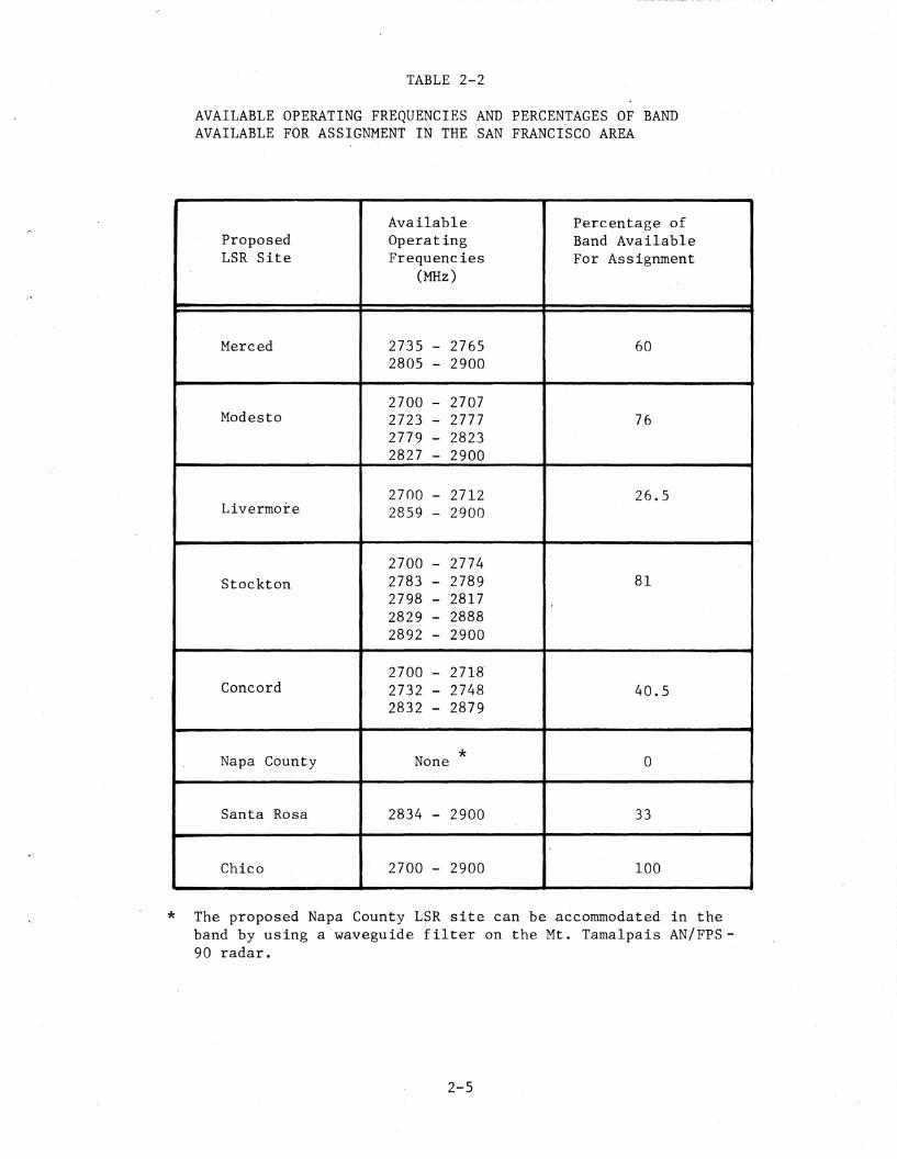
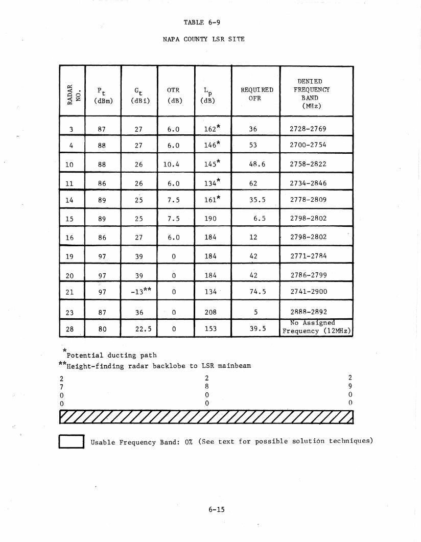
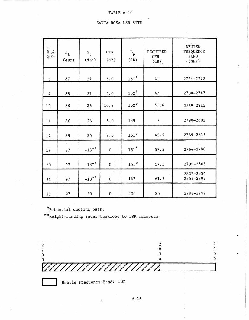
1. TABLE 2-2 shows the available operating frequencies andpercentage of the 2 .7 to 2 •9 GHz band u,sable for frequencyassignment for each of the proposed ~SR sites. LSRs can bedeployed at seven of the eight proposed sites without performancedegradation to the existing radars in the environment, or theLSRs. The proposed LSR site at Napa County could potentiallyreceive illterferenc'e from radars in the San Francisco area regardless of its operating frequency in the 2.7 to 2.9 GHz band.
2. The proposed LSR site at Napa County Airport is located near theNorth end of the San Francisco/San Pablo Bay. Propagationducting phenomena, which occurs approximately 50 percent of thetime in the summer in the Bay area, significantly decreases thepercentage of the band available for operation of an LSR at theNapa County Airport. Also the Mt.· Tamalpais height-findingradar, which is line-of-sight with the proposed LSR site"deniesthe Napa County Airpor't LSR approximately 79.5 percent of the 2 .7to 2.9 GHz band. In order to accommodate an LSR at the proposedNapa County' Airport site, it is anticipated that a waveguidefilter may be required on the Mt. Tamalpais height-finding radar.
2-4
TABLE 2-2
AVAILABLE OPERATING FREQUENCIES AND PERCENTAGES OF BANDAVAILABLE FOR ASSIGNMENT IN THE SAN FRANCISCO AREA
Available Percentage ofProposed Operating Band AvailableLSR Site Frequencies For Assignment
(MHz)
Merced 2735 - 2765 602805 - 2900
2700 - 2707Modesto 2723 - 2777 76
2779 - 28232827 - 2900
2700 - 2712 26.5Livermore 2859 - 2900
2700 - 2774Stockton 2783 - 2789 81
2798 - 28172829 - 28882892 - 2900
2700 - 2718'Concord 2732 - 2748 40.5
2832 - 2879
Napa County None * 0
Santa Rosa 2834 - 2900 33
Chico 2700 - 2900 100
* The proposed Napa County LSR site can be accommodated in theband by using a waveguide filter on the Mt. Tamalpais AN/FPS90 radar.
2-5
RECOMMENDATIONS
Considering the findings resulting from the Los Angeles and San Franciscoarea LSR deployment investigation, the following action is recommended:
1. Because of the level of usage of the 2.7 to 2.9 GHz band incertain area.s within CONUS and the uncer~ainty in requirements ofnew systems in the band, a.n investigation' of the feasibility ofaccommodating the combined requirements of the ASR-9,NEXRAD, andLSR should be conducted. This investigation should be based onGovernment agency projected requirements in the 2.7 to 2.9 GHzband.
2. An IRAC Technical Subcommittee (TSC) Ad Hoc group should be established to determine system performance guidelines required for newprocurements in the 2.7 to 2.9 GHz band. These performance guidelines sho\uld be directed towards:
a. Identifying more stringent RSEC criteriater emission spectrum sideband levelsadjacent channel interference.
for radar transmitin order to minimize
b. Defining the environmental signal characteristics which newradar systems may have to contend with in performing theiroperational requirements. The environmental signalcharacteristics should be in terms such as: pulse width, PulseRepetition Frequency (PRF), and expected signal levels. TOisinformation can then be used as a per'formance guideline indeveloping receiver interference suppression techniques.
c. Developing a compendium for reference of interference suppression techniques and their significant charactristics.
3·. An IRAC Spectrum Planning Subcommittee (SPS) Ad Hoc group shouldbe established to assure that new systems are properly engineeredto enhance their accommodation in the 2.7 to 2.9 GHz band. TheS·PS Ad Hoc group activities should be directed towards:
a. The iden~ification of Government agency procurement plans inthe 2.7 to 2.9 GHz band through 1985.
b. The over-sight a·f the implementation of the performance guidelines established by the TSC Ad Hoc group in new systems.
4. An investigation into the spurious emission characteristics of thecoaxial magnetrons used in the height-finding radars should beconducted to determine why the coaxial magnetron emiss'ion spectraare not as clean as purported.
5. In congested, areas, the secondary radiolocatian height-findingr'adar transmitters should use some method (waveguide fil ter, etc.)of controlling their spurious emission spe'ctra levels in order thatthey do not deny a large percentage of the band to other users.
2-6
6. A measurement program should be conducted to determine thecapability of doppler radars planned for the 2.7 to . 2.9 GHz bandto suppress asynchronous pulsed interfereqce under actual fieldoperating conditions.
7. The NEXRAD radar should be designed, if practical, to operate on asingle frequency. In view of the congestion in this band,itis believed that the joint development'group should seriouslyconsider this possibility before they proceed with a dual frequencysystem. A single frequency system is much more likely to be accommodated in heavily used areas.
8. Priority be given to replacing the ASR-4, ASR-5, and ASR-6 radarsin congested areas with the ASR-9 system.
9. Because of the congestion being experienced in this band andbecause of the safety-of-life nature of the aeronautical radionavigation service, all new or replacement radars operating in the2700 to 2900 MHz band in the primary aeronautical radionavigationor meteorological aids services or the secondary radiolocation service should be reviewed in the SPS.
10. All new radar p~ocurements in the 2.7 to 2.9 GHz band be requiredto submit measured data on Form OT-33, 34, and 35 for stage 4Systems Review approval.
2-7
SECTION 3
LSR SYSTEM CHARACTERISTICS AND DESCRIPTION
INTRODUCTION
This'section contains a discussion of the LSR syst~m characteristics, andsystem desc~iption. An analysis of the signal processing ofasychronous pulsedinterference through the LSR receiver, and appropriate performance criteria forthe L"SR in an asynchronous pulsed interference environment "are given inAppendix B.
BACKGROUND
Present design plans for the LSR are to use the Moving Target Detection(MTD) signal processing technique. In 1975, a hard-wired version of the MrDwas tested extensively at the National Aviation Facillties Experimental Center(NAFEC) near Atlantic City. The subclutter visibility performance of the MTDon controlled aircraft flying in heavy rain and ground clutter was measured tobe about 100 times (20dB) greater than conventional Moving Target Indicator(£VITI) performance. The {vITD employs coherent, linear doppler fil tering,adaptive thresholding, and a fine grained clutter map to reject ground clutter,rain Clutter, angels (birds) and interference. A detailed discussion of theoriginal MTD radar (MTD-I) signal processing is given by O'Donnell, M~ehe,
Labitt, Drury and Cartledge (19'/4); Drury (1975) and ·Cartledge and O'J)onnell( 191 f7) •
In June 1979 a second generation MrD radar (MTD-II) was installed atBurlington Vermont for operational field evaluation~ The major differencebetween the MTD-I and MTD-II radars are the methods used to implement thedoppler filtering. The MTD-I used an eig~t point 'Discrete Fourier Transform(DFT) fbr the doppler filters, while the MID-II use~ Finite Impulse Response(FIR) filters, often called transversal filters. A discussion of the MID-II isgiven by O'Donnell and Muehe (1979).
SlSIEM CHARACTERISIICS
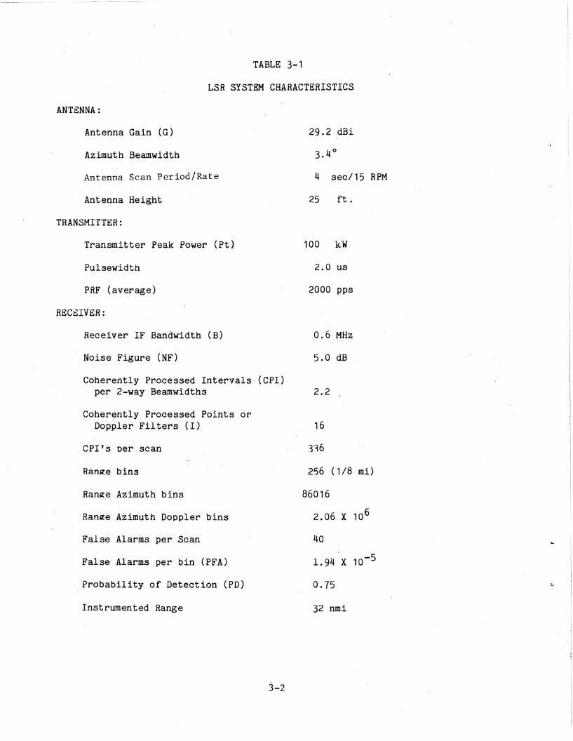
TABLE 3-1 shows a list of the basic system chara~teristics proposed forthe LSR. Since the LSR system is still in the developmental phase, and theMTD-II signal processing technique is still undergoing operational fieldevaluation, the LSR system ch·aracteristics shown in TABLE 3-1 may not berepresentative of the final procurement specifications for the LSR system.
The major difference between proposed LSR characteristics and the MID-IIbeing evaluated at Burlington is the implementation of 16 doppler filtersrather than eight doppler filters. Other possible changes to the MTD-IIprocessor which may be incorporated in the LSR are discu~sed in the followingsystem description. Since the threshold criteria for a 16 doppler filter MTOradar have not been determined, the following system description is for theeight doppler MID-II system.
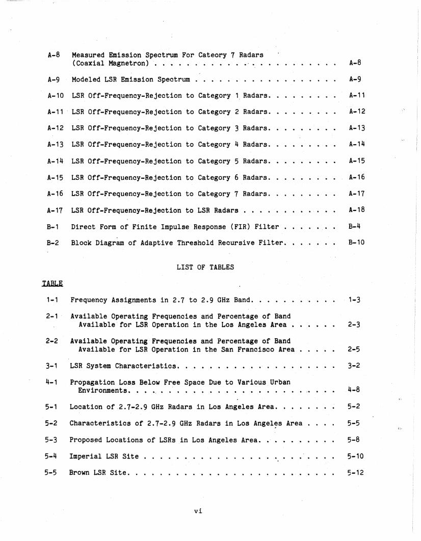
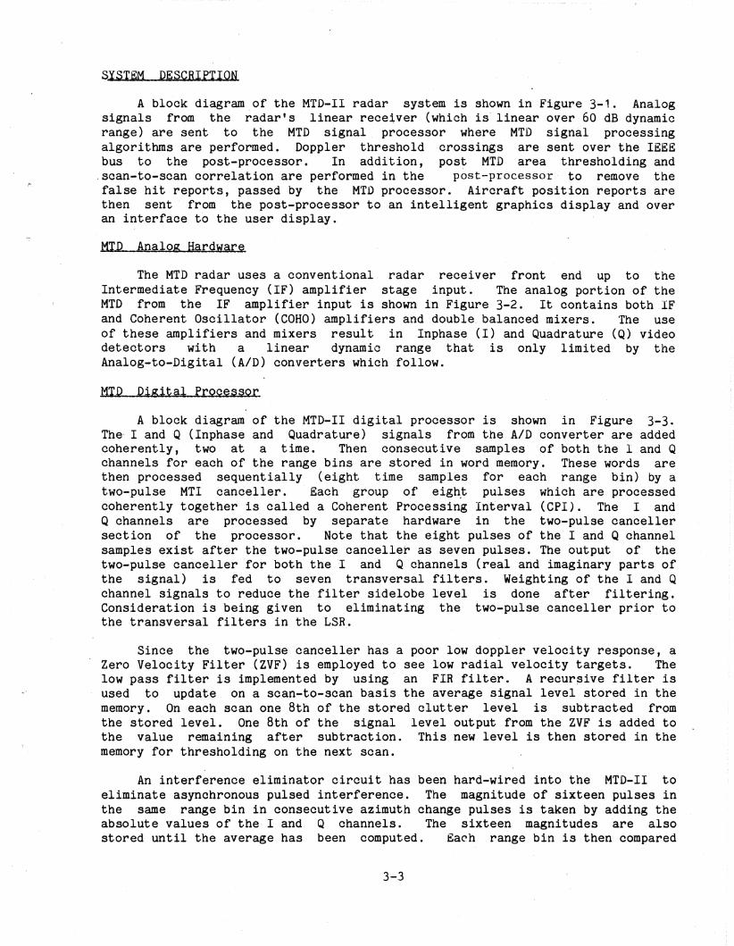
A block diagram of the MTD-II radar system is shown in Figure 3-1. Analogsignals from the radar's linear receiver (which is' linear over 60 dB dynamicrange) are sent to the MTD signal. processor where MTD signal processingalgorithms are performed. Doppler threshold crossings are sent over the IEEEbus to the post-processor. In addition, pos~ MTD area thresholding and
.scan-to-scan correlation are performed in the post--processor to remove thefalse hit reports, passed by the MTD processor. Aircraft position reports arethen sent from the post-processor to an intelligent graphics display and overan interface to the user display.
MTD Analog Hardware
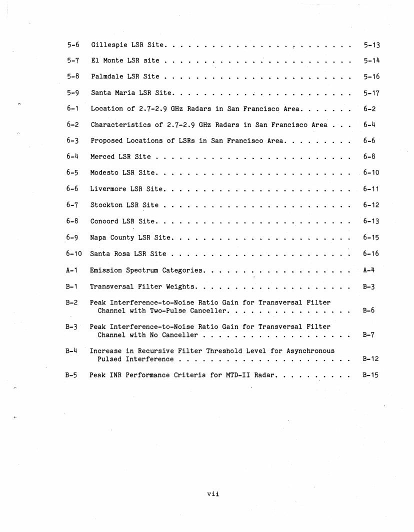
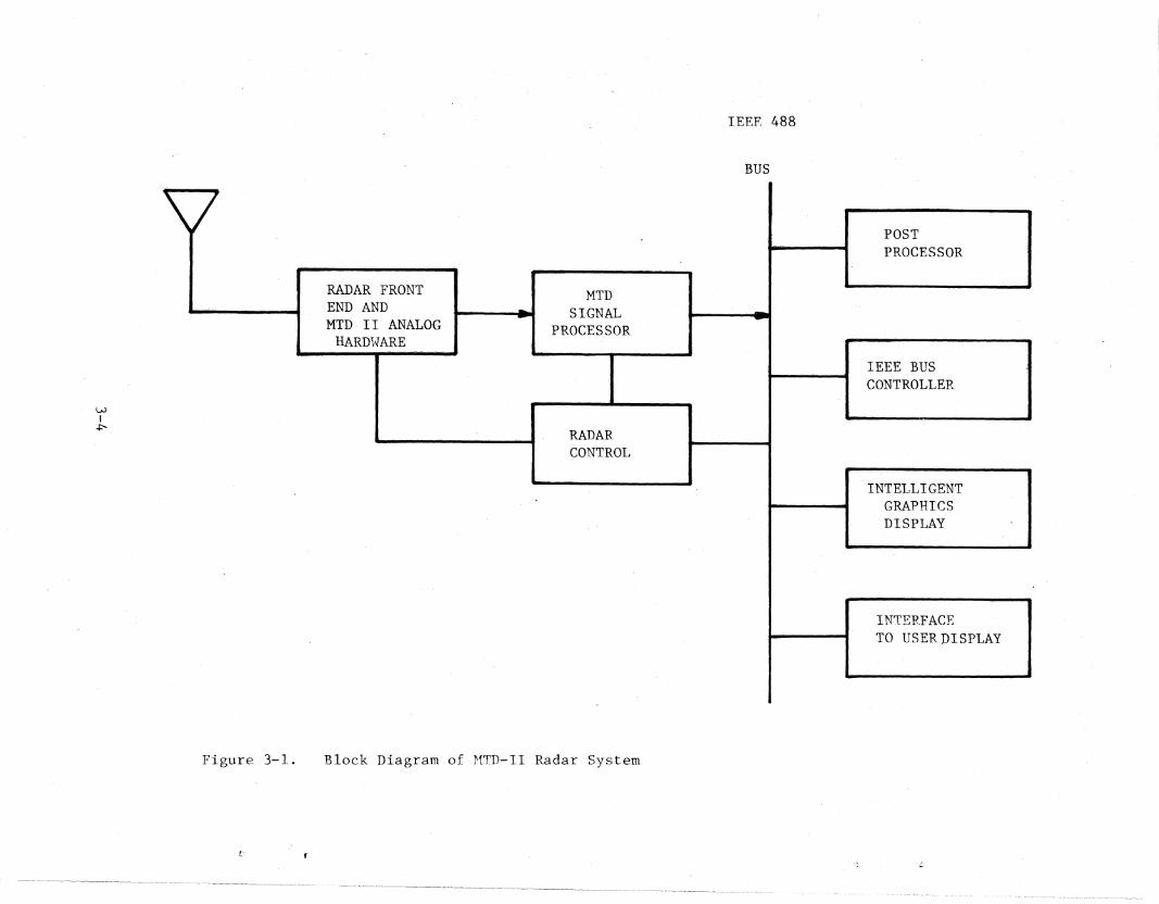
The MTD radar uses a conventional radar receiver front end up to theIntermediate Frequency (IF) amplifier stage input. The analog portion of theMTD from the IF amplifier input is shown in Figure 3-2. It contains both IFand Coherent Oscillator (COHO) amplifiers and double. balanced mixers. The useof these amplifiers and mixers result in Inphase (I) and Quadrature (Q) videodetectors with a linear dynamic range that is only limited by theAnalog-to-Digital (AID) converters which follow.
MID Digital Processor
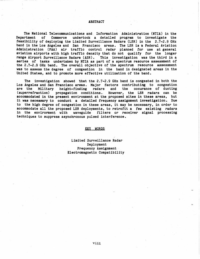
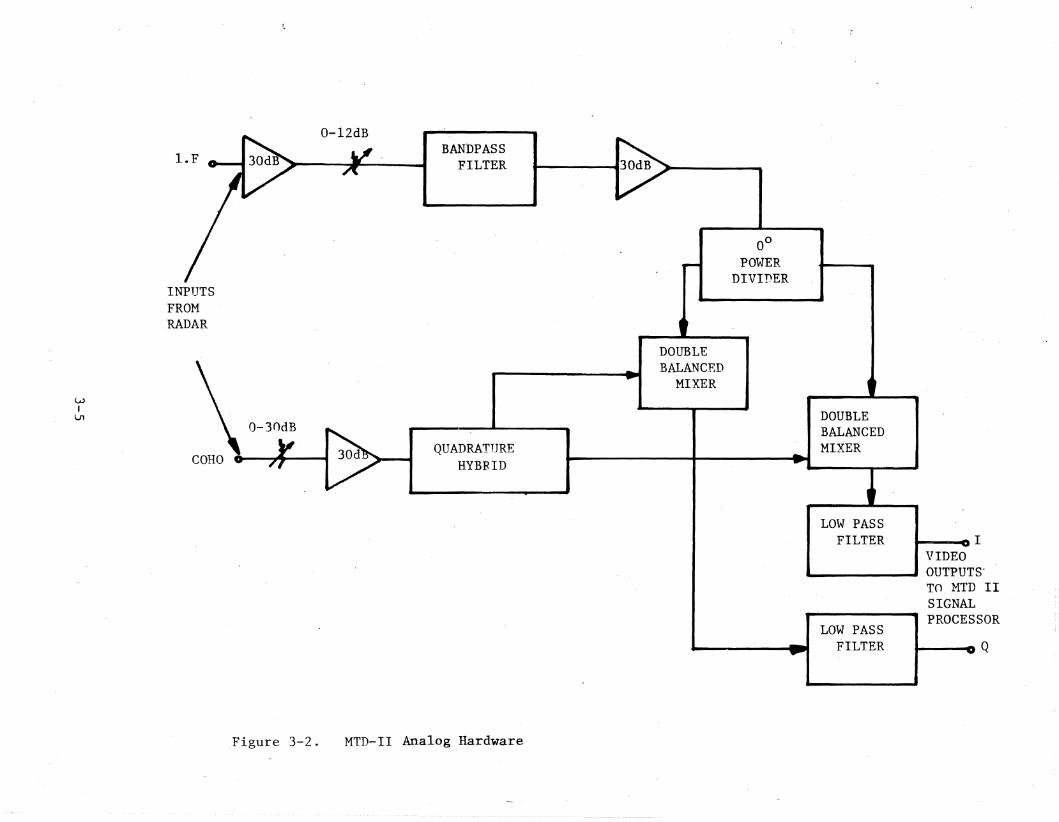
A block diagram of the MTD-II digital processor is shown in Figure 3-3.The- I and Q (Inphase and Quadrature) signals from the AID converter are addedcoherently, two at a time. Then consecutive samples of both the I and Qchannels for each of the range bins are stored in word memory. These words arethen processed sequentially (eight time samples for each range bin) by atwo-pulse MTI canceller. Each group of eigh~ pulses which are processedcoherently together is called a Coherent Processing Interval (CPI). The I andQ channels are processed by separate hardware in the two-pulse cancellersection of the processor. Note that the eight pulses of the I and Q channelsamples exist after the two-pulse canceller as seven pulses. The output of thetwo-pulse canceller for both the I and Q channels (real and imaginary parts ofthe signal) is fed to seven transversal filters. Weighting of the I and Qchannel signals to reduce the filter sidelobe level is done after filtering.Consideration is being given to eliminating the two-pulse canceller prior tothe transversal filters in the LSR.
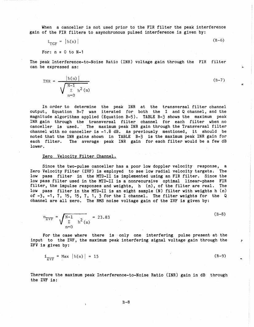
Since the two-pulse canceller has a poor low doppler velocity response, aZero Velocity Filter (ZVF) is employed to see low radial velocity targets. Thelow pass filter is implemented by' using an FIR filter. A recur~ive filter isused to update on a scan-to-scan basis the average signal level stored in thememory. On each scan one 8th of the stored clutter level is subtracted fromthe stored level. One 8th of the signal level output from the ZVF is added tothe value remaining after subtraction. This new level is then stored in thememory for thresholding on the next scan.
An interference eliminator circuit has been hard-wired into the MTD-II toeliminate asynchronous pulsed interference. The magnitude of sixteen pulses inthe same range bin in consecutive azimuth change pulses is taken by adding theabsolute values of the I and Q channels. The sixteen magnitudes are alsostored until the average has been computed. Each range bin is then compared
3-3
LVI~
IEEE 488
BUS
\/ POSTPROCESSOR
RADAR FRONT MTDEND AND ........ SIGNAL .........--MTD I I ANALOG PROCESSORHARD~\iARE
IEEE BUSCONTROLLEP..
I I
RADARCONTROL
INTELLIGENTGRAPHICSDISPLAY
I!'lTER.FACETO USER DISPLAY
Figure 3..... 1.
l:
Block Diagram of ~1TD-II Radar System
INPTJTSFROMRADAR
0-12dBBANbPASS
FILTER
0°POWER
DIVIDER
wI
U1
QUADRATTJREHYBRID
DOUBLEBALANCED
MIXER
DOUBLEBALANCEDMIXER
LOW PASSFILTER
LOW PASSFILTER
I "IVIDEOOUTPUTS'TO MTD IISIGNALPROCESSOR
I nQ
Figure 3-2. MTD-II Analog Hardware
R(1) AZIMUTH(2) RANGE(3) VELOCITY(4) AMPLITUDE
8 PULSES RAIN ANDAID I and Q 2 - Pulse GENERALIZED WEATHER
Figure 3-3. Block Diagram of MTD-II Signal Processor
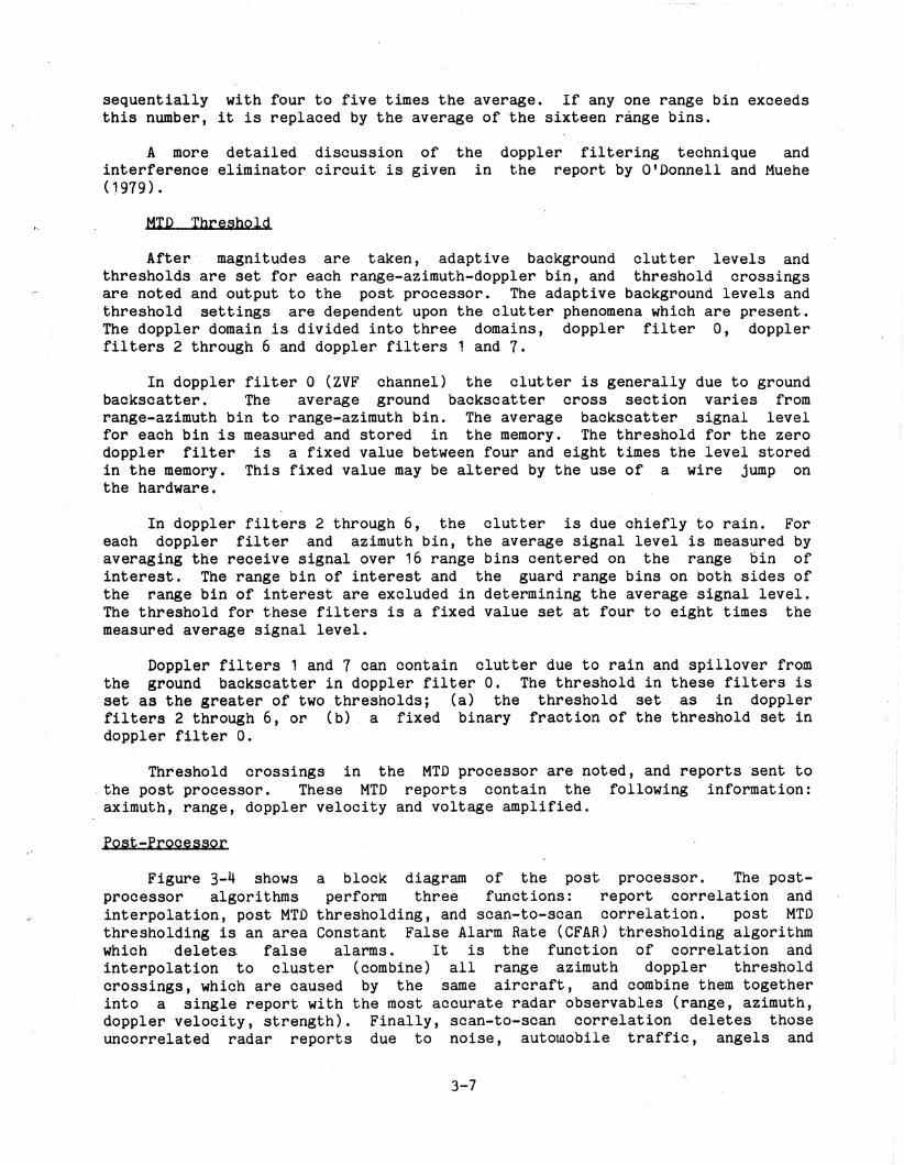
sequentially with four to five times the average. If anyone range bin exceedsthis number, it is replaced by the average of 'the sixteen range bins.
A more detailed discussion of theinterference eliminator circuit is given in(~979).
MID Tbre§hold
doppler filtering technique andthe report by O'Donnell and Muehe
After' magnitudes are taken, adaptive background clutter levels andthresholds are set for each range-azimuth-doppler bin, and threshold crossingsare noted and output to the post processor. The adaptive background levels andthreshold settings are dependent upon the clutter phenomena which are present.The doppler domain is divided into three domains, doppler filter 0, dopplerfilters 2 through 6 and doppler filters 1 and 1.
In doppler filter 0 (ZVF channel) the clutter is generally due to groundbackscatter. The average ground backscatter cross section varies fromrange-azimuth bin to range-azimuth bin. The average backscatter signal levelfor each bin is measured and stored in the memory. The threshold for the zero
-doppler filter is a fixed value between four and eight times the level storedin the memory. This fixed value may be altered by the use of a wire jump onthe hardware.
In doppler filters 2 through 6, the clutter is due'chiefly to rain. Foreach doppler filter and azimuth bin, the average signal level is measured byaveraging the receive signal over 16 range bins centered on the range bin ofinterest. The range bin of interest and the guard range bins on both sides ofthe range bin of interest are excluded in determining the average signal level.The threshold for these filters is a fixed value set at four to eight times themeasured average signal level.
Doppler filters 1 and 7 can contain clutter due tC) rain and spillover fromthe ground backscatter in doppler filter'O. The threshold in these filters isset as the greater of two thresholds; (a) the threshold set as in dopplerfilters 2 through 6, or (b) a fixed binary fraction of the threshold set indoppler filter O.
Threshold crossings in the, MTD processor are noted, and reports sent to. the post processor. These MTD reports contain the following information:aximuth, range, doppler velocity and voltage amplified.
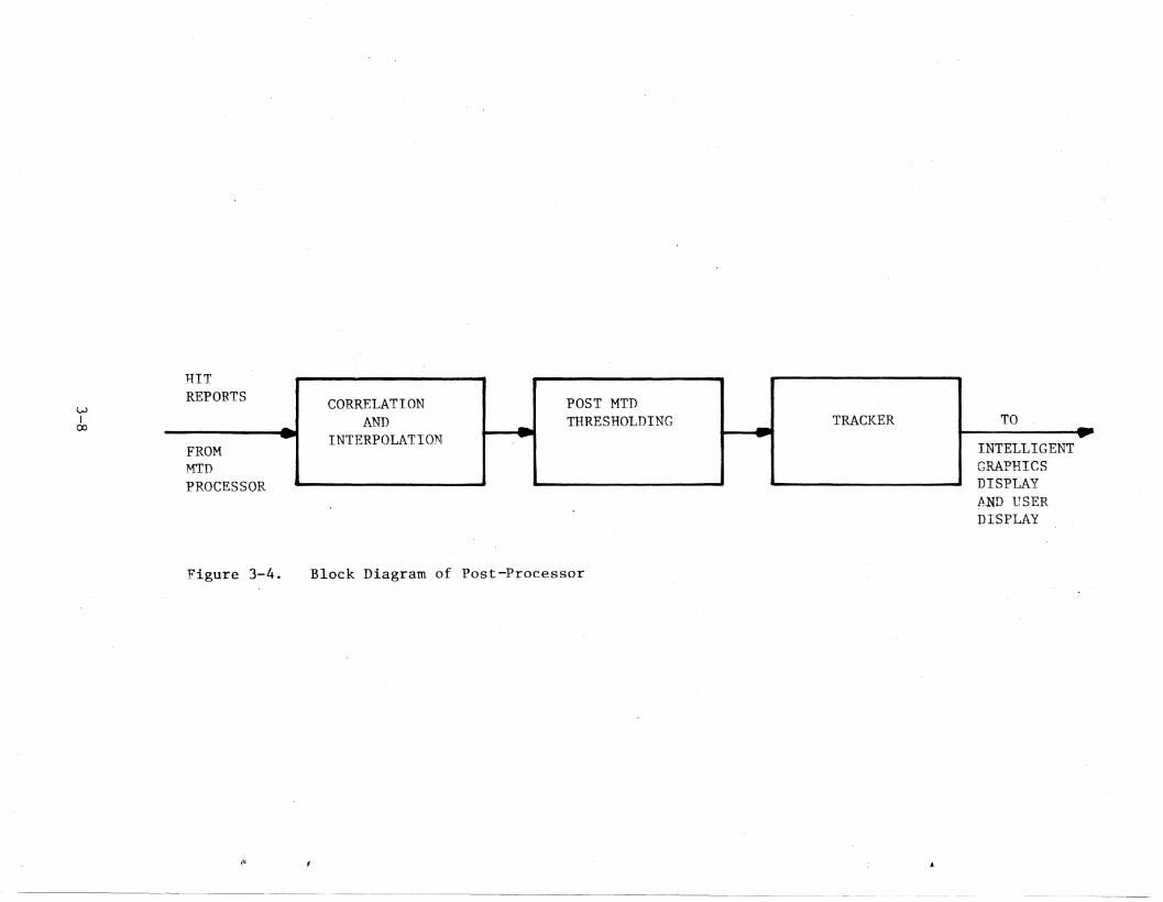
Post-frocessor
Figure 3-4 shows a block diagram of the post processor. The postprocessor algorithms perform three functions: report correlation andinterpolation, post MTD thresholding, and scan-to-scan correlation. post MTDthresholding is an area Constant False Alarm Rate (CFAR) thresholding algorithmwhich deletes. false alarms. It is the function of correlation andinterpolation to cluster (combine) all range azimuth doppler thresholdcrossings, which are caused by the same ai.rcraft, and combine them togetherinto a single report with the most accurate radar observables (range, azimuth,doppler velocity, strength). Finally, scan-to-scan correlation deletes thoseuncorrelated radar reports due to noise, autowobile traffic, angels and
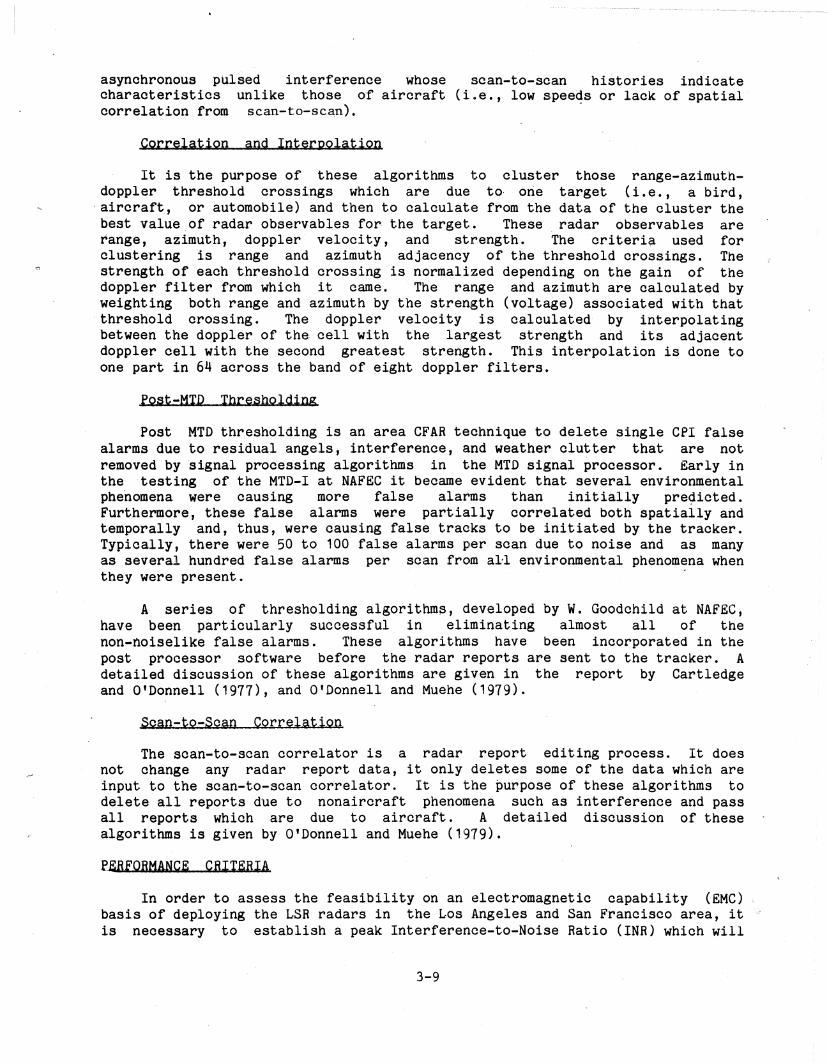
asynchronous pUlsed interference whose scan-to-scan histories indicatecharacteristics unlike those of aircraft (i _, e ., low speeqs or lack of spatialcorrelation from scan-to-sc~n).
Correlation and Interpolation
It is the purpose of these algorithms to cluster those range-azimuthdoppler threshold crossings which are due to· orie target (i.e., a bird,
. aircraft., or automobile) and then to calculate from the data of the cluster thebest value.of radar observables for the target. These radar observables arerange, azimuth, doppler velocity, and strength. The criteria used forclus~ering is range and azimuth adjacency of the threshold crossings. Thestrength of each threshold crossing is normalized depending on the gain of thedoppler filter from which it came. The range and azimuth are calculated byweighting both range and azimuth by the strength (voltage) associated with thatthreshold crossing. The doppler velocity is calculated by interpolatingbetween the doppler of the cell with the largest strength and its adjacentdoppler cell with the second greatest strength. This interpolation is done toone part in 64 across the band of eight doppler filters.
Post-MTD Thr§sholding
Post MTD thresholding is an area CFAR technique to delete single CPI falsealarms due to residual angels, interference, and weather clutter that are notremoved by 'signal p~ocessing algorithms in the MTD signal processor. Early inthe testing of the MTD-I at NAFEC it became evident that several environmentalphenomena were causing more false alarms than initially pre~icted.
Furthermore, these false alarms were partially correlated both spatially andtemporally and, thus, were causing false tracks to be initiated by the tracker.Typically, there were 50 to 100 false alarms per scan due to noise and as manyas several hundred false alarms per scan from a~l environmental phenomena whenthey were present. ~
A. series of thresholding algorithms, developed by W. Goodchild at NAFEC,have been particularly successful in eliminating almost all of thenon-noiselike false alarms. These algorithms have been incorporated in thepost processor software before the radar reports are sent to the tracker. Adetailed discussion of these algorithms are given in the report by Cartledgeand O'Donnell (1977), and O'Donnell and Muehe (1979).
Scan-to-Scan CorrelatiQD
The scan-to-scan correlator is a radar report editing process. It doesnot change any radar report data, it only deletes some of the data which areinput to the scan-to-scan correlator. It is the purpose of these algorithms todelete all reports due to nonaircraft phenomena such as interference and passall reports which are due to aircraft. A detailed discussion of thesealgorithms is given by O'Donnell and Muehe (1919).
fERFORHANCE CRITERIA
In order to assess the feasibility on an electromagnetic capability (EMC)basis of deploying the LSR radars in t.he Los Angeles and San Francisco area, itis necessary to establish a peak Interference-to-Noise Ratio (INR) which will
3-9
preclude performance degradation of the LSR System.. F',or ·this investigation,the criteria used to establish an appropriate peak INi was:
1. The level of interference should not cause false hit reportsto De sent to the MTD post~processor whicb could result inoverloading of the post-processor.
2. The level of interference should not cause the MfD threshhold level to be increased by more than 1 dB.
An analysis of the signal processing of asynchronous pulse4 interferencethrough the LSfl receiver, and appropriate performance criteria for the L3rl inan asynchronous pulsed interference environment are given in Appendix B. It isshown in Appendix B that a peak INrl of 5 dB will preclude performancedegradation to the LSR.
3-10
SECTION 4
FREQUENCY ASSIGNMENT PROCEDUR~
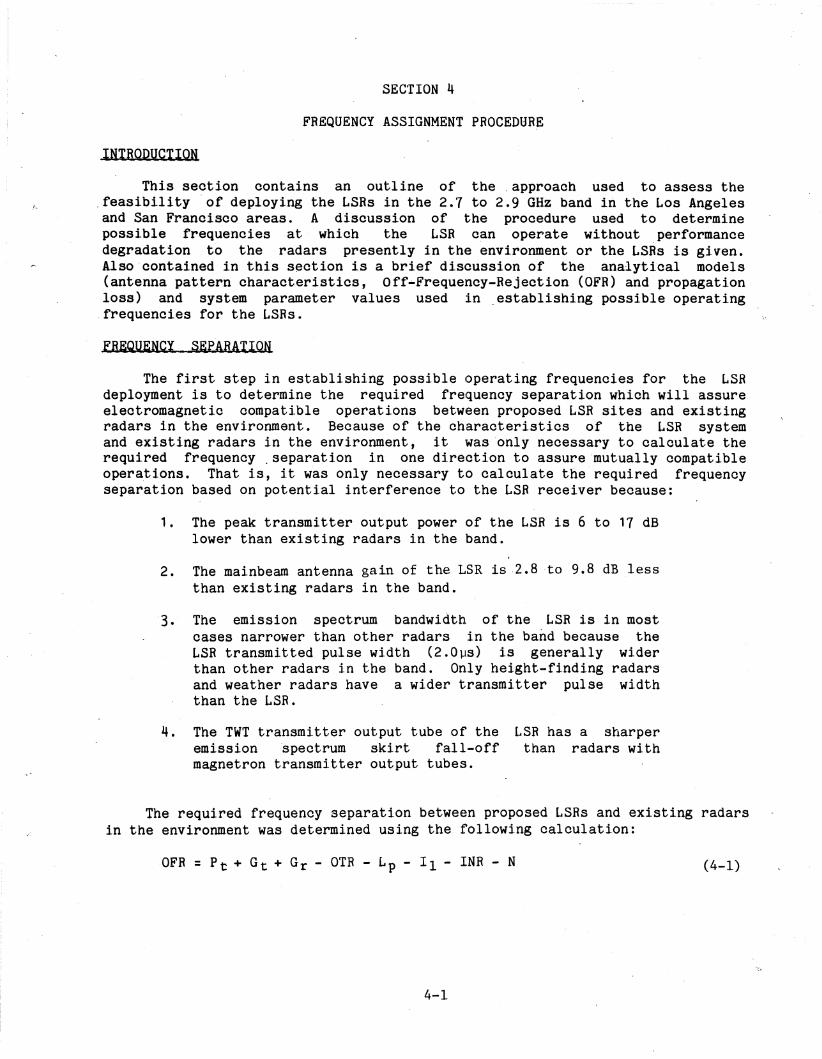
This section contains an outline of the .approach used to assess the.feasibility 'of deploying the LSRs in the 2.7 to 2.9 GHz band in the Los Angelesand San Francisco areas. A discussion of the procedure used to determinepossible frequencies at which the LSR can operate without .performancedegradation to the radars presently in the environment or the LSRs is given.Also 'contained in this section is a brief discussion of the analytical models(antenna pattern characteristics, Off-Frequellcy-Rejection (OFR) and propagationloss) and system parameter values used in .establishing possible operating
. frequencies for the LSRs.
The first step in establishing possible operating frequencies for the LSRdeployment is to determine the required frequency separation which will assureelectromagnetic compatible operations between proposed LSR sites and existingradars in the environment. Because of the characteristics of the LSR systemand existing radars in the environment, it was only necessary to calculate therequired frequency ,separation in one direction to assure 'mutually compatibleoperations. That is, it was only necessary to calculate the required frequencyseparation based on potential interference to the LSR receiver because:
1. The peak transmitter output power of the LSR is 6 to 17 dBlower than existing radars in the band.
2. The mainbeam antenna gain of the LSR is .2.8 to 9.8 dB lessthan existing radars in the band.
'3. The emission spectrum bandwidth of the LSR is in mostcases narrower than other radars in the band because theLSR transmitted pulse width (2.0~s) is generally widerthan other radars in the band. Only height-finding radarsand weather radars have a wider transmitter pulse widththan the LSR.
4. The TWT transmitter output tube of theemission 'spectrum skirt fall-offmagnetron transmitter output tubes.
LSR has a sharperthan radars with
The required frequency separation between proposed LSRs and existing radarsin the environment was determined using the following calculation:
OFR = Pt + Gt + Gr - OTR - LP - II - INR - N
4-1
(4-1)
where:
OFR' = The required off~frequency-rejectionbetween the LSRreceiver and the potential ~nterfering radar, in 4B(OFR > 0)
P t = The transmi t tel' power of the'interfering radar, in dBm
potential
Gt = The nominalfering(mainbeam
mainbeam gain of the potential interminus correction for antenna tilt angle
to -12 dB), in dBi
Gr = LSR antenna median backlobe level, -12 dBi
OTR = The on-tune ection of the interfering signal dueto the LSR receiver bandwidth being narrower thanthe interfering signal emission bandwidth, (OTR = 20log B T) in dB (B =: LSR IF bandwidth, and T = interfering pulse width)
= Median propagation path loss between LSR and potential interfering radar, in dB
1'1 = Waveguide and coupler insertion losses of both LSRand potential interfering radars. A 2 dB insertionloss was used at both ends (Offi and Herget, 1968).
INR = Maximum allowable peak Interference-to-Noise Ratioat the LSR receiver input to preclude LSR performance degradation? 5 dB (See Appendix',B)
N = LSR receiver inherent noise level referred to the RFinput, (N = ~114 + 10 log B{MHz)+ NF) = -111 dBm)
Using the fixed parameter values discussed above, Equation 4-1 can be expressedas:
O~R = P t + Gt ~.. OTH -- Lp + 90 (4-2)
Equation 4-2 was used to calculate the Off-Frequency-Rejection (OFR). except in some cases of mainbeam coupling from height-finding radars.Generally height-finding radar mainbeam antenna coupling to aeronauticalradionavigation radars does not occur period~cally because the antenna onheight-finding radar~ does not rotate 360 degrees at a constant RPM rate.However, height-find radar mainbeam coupling to aeronautical radars doesoccur occasionallyQ Because of the high power and antenna gain ofheight-finding radars~ in some cases it is difficult to preclude performancedegradation from height~finding radars without denying an LSR a largepercentage of' the 2$"'{ to 2 . 9 GHz band. Therefore, in some cases antennacoupling of the LSR mainbeam to the height-finding radar backlobe was used.For this situation, an LSR mainbeam antenna gain (G r ) of 22.2 dBi {29.2 dBi -1
4-2
dB for tilt angle) and a heignt-finding backlobe antenna gain (G t ) of -13 dBiwas used.
Once the required OFR was calculated; the required frequency separationbetween "the LSR operating frequency and the operating frequency of thepotential interfering radar was determinded usi.ng an analytical OFR model (CCIRReport 654) •. After the required frequency separation between theLSR andradars pr~sently in the environment was determined, appropriate operatingfrequencies .for theLSR to operate were indicated in a bar graph along with thepercentage of the 2. 7 to 2.'9 GHz band available for LSR operation.
The following is a brief discussion of the analytical models (antennapattern characteristics, Off-Frequency-Rejection (OFR) and propagation loss)
. used in establishing possible operating frequencies for the LSR.
Ant~nna. Eatterns
A three level antenna pattern statistical model for an average clutterarea was used to determine operating frequencies for the LSR in the Los Angelesand San Francisco areas.' The statistical antenna characteri,stics were obtainedby measuring antenna patterns of radars ·in the 2.7 to 2.9GHz band ~sing theNT!A Radio Spectrum Measurement System (RSMS) van (Hinkle, ·Pratt and Matheson,1976). The statistical median antenna gain, standard dev'iation (0) and degreesfor each of these regions are:
Mainbeam Region: Gain: Nominal mainbeam gain minus correctionfor antenna tilt angle
Degrees: 351 0 to 3 0
Sidelobe Region: Gain: -7 dBi, a = 3 dB
Backlobe Region: Gain: -13 dBi, a = 3dB
Degrees: 25 0 to 335 0
Surveillance radars with cosecant squared elevation antenna patternsnormally tilt the mainbeam of the· radar above the horizon to r~duce ground.clutter, therefore, the antenna gain at an elevat~on angle of zero degrees maybe typically 5 to 12 dB below the actual mainbeam gain. For example, the' FAAAirport Surveillance Radars (ASRs) have a nominal mainbeam gain of 34 dBi, anda typical antenna tilt angle of 3.0 to 3.5 degrees. The antenna gain along thehorizon for an antenna tilt angle of 3.0 to 3.5 degrees is ~pproximately sevendB down from the nominal mainbeam gain. ThUS, the mainbeam antenna gain alongthe horizon for ASRs is typically 27 dBi.
The mutual antenna gain coupling considered for this i.nvestigation wasmainbeam-to-backlobe. Mainbeam-to-mainbeam antenna gain coupling may occur in
4-3
the environment. However, the percentage of time mainbeam~to-mainbeamcouplingmay occur is less than .01' percent. BeOause the pr~sent radars in theenvironment have a mainbeamgain of 2.8 to 9.8 dB grea~er than the proposed LSRantenna, the mainbeam of. the radars in .the environment (interfering radars) tothe LSR median backlobe level of ~12 dBi was used. The LSR median backlobelevel of -12 dBi was based on a measured median backlobe level of -13 dB forthe larger ASR antennas. For example, the mutual antenna gain coupling formainbeam of' an ASR to the backlo~e of the LSR would be +15 dBi (+ 27 dBi - 12 •dBi). The probability of the coupled mutual antenna gain exceeding + 15 dBi isapproximately 1.3 percent (Hinkle, Pratt, Matheson, 1976). This is aconservative mutual antenna gain coupling criteria since it implies that only1.3% of the time the interfering signal level will exceed the- INR = 5 dBperformance criterion. .
Qff-=.FrequencY-..Be i~ct iQn
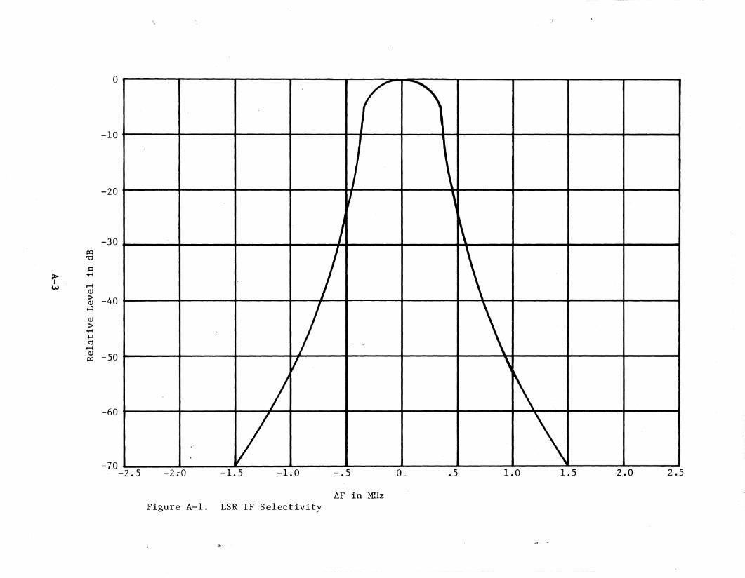
The Off-Frequency Rejection (OFR) model accounts for the energy couplingloss of an undesired signal in a victim receiver due to the frequencyseparation between the interfering radar transmitter operating frequency andthe victim radar receiver tuned frequency. Therefore, the OFR model is anecessary component in predicting the level of interference at a radar receiverIF output. The factors, which affect the OFR of a victim receiver are thevictim receiver IF selectivity, interfering signal emission spectrumcharacteristics and .the frequency separation between the interfering and victimradars. .
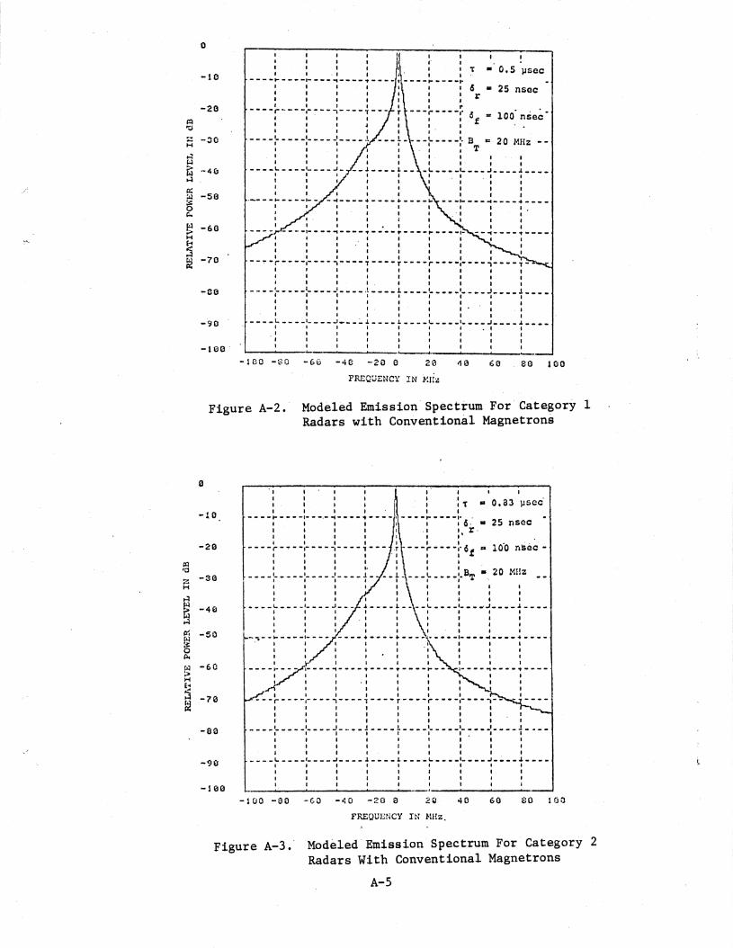
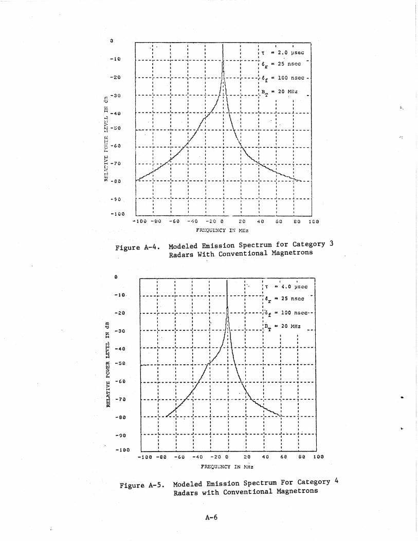
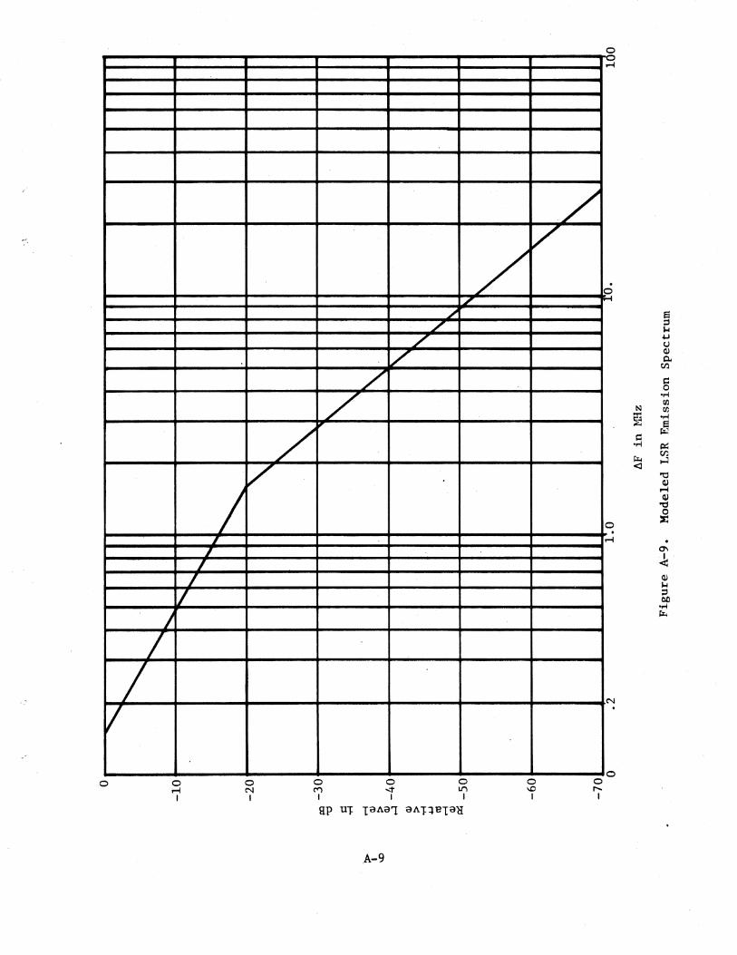
Appendi~ A contains a detailed discussion of the OFR model, LSR receiverIF selectivity and the emission spectrum characteristics used to representradars in the 2.1 to 2.9 GHz band. An analytical model (Newhouse, 1969) wasused to obtain the emission spectrum characteristics of radars usingconventional magnetron transmitter output tubes. Measurements made with theRSMS van were used to validate the conventional magnetron emission spectrummodel (Hinkle, Pratt, Matheson, 1976). The RSMS van was also used to measureemission spectrum characteristics of new radars in the 2.'7 to 2.9 GHz bandwhich. use diplex filtered conventional magnetrons," coaxial magnetrons andklystron transmitter output tubes.
A compendium of OFR curves used to determine the feasibiliy of deployingthe LSR in the 2.7 to 2.9 GHz ban~ in the Los Angeles and San Francisco areas~re also contained in Appendix A.
The prediction of the pr~pagation path ·loss between the potentialinterfering transmitter radar sites and the proposed LSR sites was obtainedusing the Terrain Integrated Rough Earth Model (TIREM) (Weissberger and Baker,1918). The TIREM propagation model is a batch program normally used to computebasic propagation loss when the specific coordinates of antenna locations areknown. The program automatically addresses a terrain data base, extracts theterrain profile along the great circle path, computes geometric terrai.nparameters, and selects the lowest loss propagation mode for calculation of thebasic propagation loss. Previous propagation loss measurements (Hinkle, Pratt,
4-4
Matheson, 1976) made in the 2.7 to 2.9 GHz band iri th~.Los Angeles and SanFrancisco ,areas indicated that the TIREM propagation model and terrain database did not consider all environmental factors that' affect propagation loss.Environmental factors which must be considered in propagation loss predictionsinclude:' ducting, man-made clutter, foliage and terrain .multipath. Thefollowing is a discussion of these environmental factors, and how they weretaken into ac~ount in predicting the basic propagation loss.
Evaporation of moisture from water creates a refractive index gradient atlow heights that can refract microwave energy downward to cre~te a "guiding"effect or duct. Propagation of electro~agnetic waves in such a duct can varyfrom a near lossless situation, to signal enhancement, depending on thefrequency and intensity of the evaporation duct. The intensity of theevaporation duct is most often described in terms of "duct height" which isdefined as the height at which the modified refractivity is minimized.
Many researchers have investigated the ducting phenomenon in the SouthernCalifornia area. Bean (1959) noted that during the summer months at San Diegoand Oakland that an elevated duct is observed about 50 percent of the time.Rosenthal (1972, 1973) and Crain (1953) States that much of the coastal area ofCalifornia is usually in a moist marine layer capped by a d~y· inversion layer.The inversion layer produces ducting conditions throughout, the year and is. mostfreque,nt in the summer months. Meterological parameters were measured by NavalElectronics Labratory Center (NELC) over a five year period, for all seasonsand times of the day, in the off-shore San Diego area~ These studies indicatedthat radar range enhancement occurs 30% of the time. Bean and Cahoon (1959)report rapid horizontal changes in refractive index associated with land-seabreezes, storms and frontal passages. Other researchers have noted largediurnal variations due to land-sea breeze circulation. In the Los -Angeles area,Neiburger (1944) noted that the inversion layer undergoes significant diurnalchanges in elevation. Edlinger (1959) ,also rep6rted rapid change~ in themarine layer with time of day.
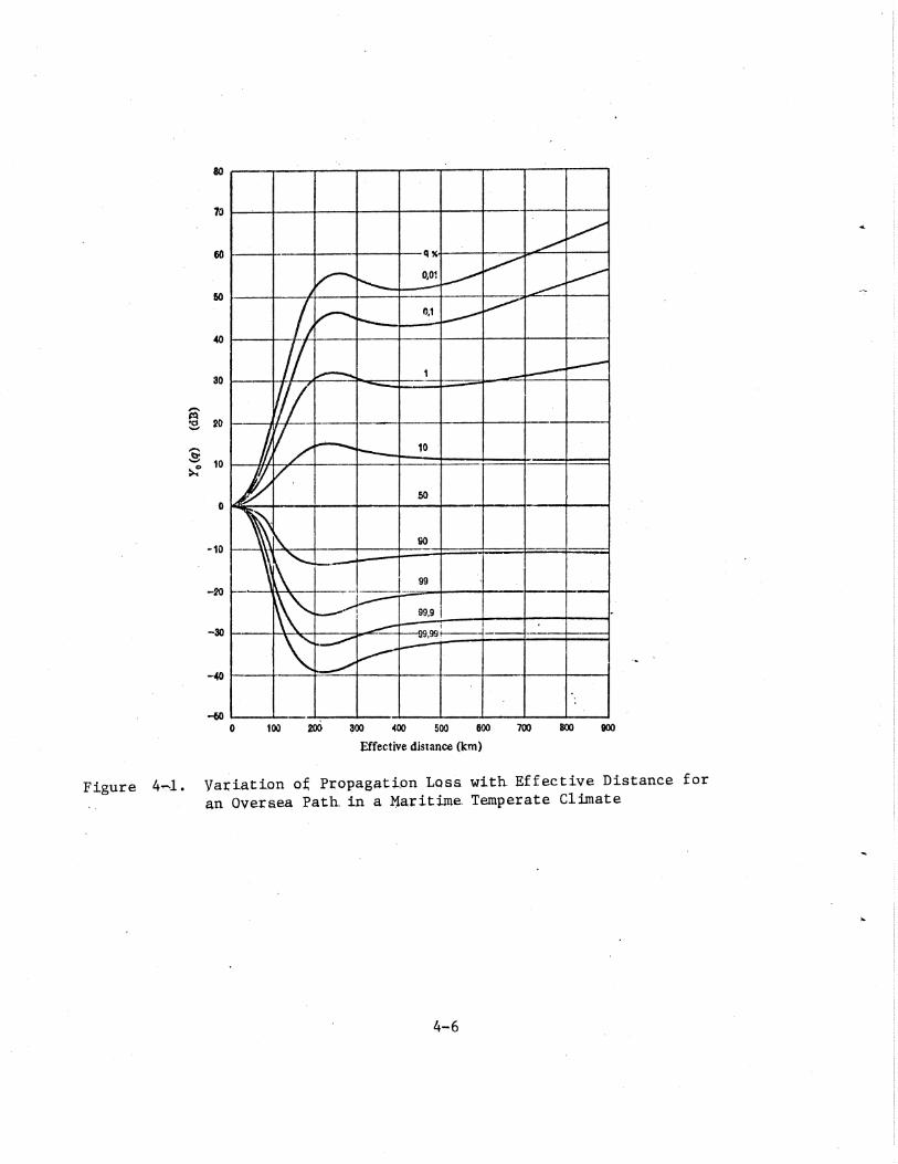
Chang (1971) concludes that when both antennas are above or within theduct, the received field is 10 to 20 dB above free space. When one or bothterminals are below the duct, the field is 10 to 25 dB below free space, evenat distances up to 1200 km. Oversea paths are more likely to be affected bysuperrefraction and elevated layers than land paths" and so give greatervariation in path loss. This may also apply to lOW, flat coastal regions in~aritime zones such as the Los Angeles and San Diego Basins. Figure 4-1 showsthe variation in transmission loss with effective distance for an ~versea pathin a maritime temperate climate (CCIR Report 238-3)".
During measurements made in the Los Angeles and San Francisco areas in1975-in the 2.7 to 2.9 GHz band (Hinkle, Pratt, Matheson 1976), it was observedthat in ducting conditions the measured propagatibn path loss wasintermittently 40 dB less than the predicted propagatiori loss, and sometimesapproached 10 dB less than free space loss. These findings were in agreementwith previous investigations and CCIR Report 238-3. Based on these measurementfindings, the procedure used in this report to take into account ducting
Figure 4~1. Va:t;iation o~ Propagati-,on Loss with- Effective Distance foran Oversea Path. in a ~aritime- Temperate Climate
4-6
phenomena over potential ducting paths was to reduce the TIREM model predictedloss by as much as 40 dB to account for the potential of ducting propagation,but not to' exceed 10 dB below "free space. Figure 4-1, shows that a propagationloss of 40 dB less than the median lev,el ma~, occur about 0.·2 percent of thetime for oversea paths in a maritim~ temperate climate. Since 0.2 percent ofthe time corresponds to less than one day a year, the 40 dB correction forpotential ducting paths is a conservative correctiqn for ducting conditions.
Man-mage Clytter
The propagation path loss through urban and surburban" areas ispredominately caused by the many multipaths due to signal.reflection anddiffraction from the man-made obstacles such as buildings. The TIREMpropagation prediction model that uses the topographical file only considersthe terrain profile in the vertical plane between the two path end points, andconsequently does not consider multipath effects due to bUilding reflectionsand diffractions.
It is believed that the most practical approach is to employ empiricalresults in selecting a man-made obstacle attenuation factor for addition to thepropagation model loss prediction. The result of the propagation loss measuredby other investigators for various degrees of built-up areas were summarized inthe report by Hinkle, Pratt and Matheson (1976).
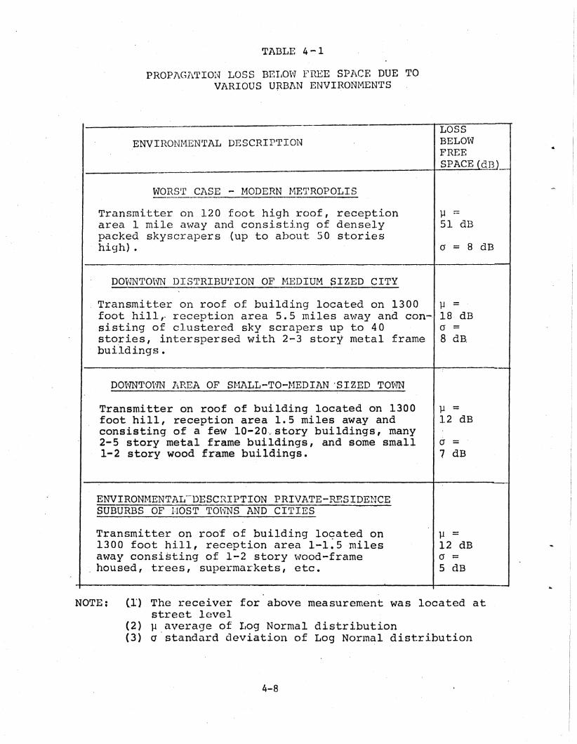
Propagation loss measurements for various degrees of building congestionin the San Francisco area were reported by Turin (1972). The environmentaldescription geometry of the test set-up, and measured median loss below freespace with standard deviation, are indicated in TABLE 4-1. These measurementswere made to support development of a statistical urban propagation model forevaluating mobile radio location performance. Th~ paths described would havebeen line-of-sight if man-made obstacles were not prE3sent. Therefore, it isassumed that the propagation losses below free space shown in TABLE 4-1, can beattributed mostly to attenuation due to buildings. The measurement resultsshown in the TABLE were made at 1280 MHz'but are reported to be very close tovalues obtained at 2920 MHz.
The results of measurements by Turin were employed in the San Franciscoarea propagation loss predictions by Hinkle, Pratt and Matheson (1976). Itresulted ,in a 7 dB improvement over the Los Angeles area predictions. The~verage difference between predicted and measured loss for San Francisco wasonly -3 dB. Based on these findings, the results by Turin were also used in-the LSR deployment investigation in the Los Angeles and San Francisco areas.
The propagation loss measurements in man-made clutter environments,referenced in the preceding section, included sparse foliage. Precisepropagation loss prediction due to trees is difficult because of variations intree type, heigpts, shape, and distribution. In addition, 'foliage density whichchanges with seasons of the year also affects attenuation. The report byHinkle, Pratt and Matheson (1976) summarizes measurements of foliageattenuation. However, for this investigation adjustments to the predictedpropagation loss values for foliage attenuation were not taken into account.
4-7
TABL:t~ 4-1
PROPl\(;I~rrI01.~ I-JOSS B.EIJO"\"1 l?REE SP]\CE~ DUE TOVARIOUS U~BAN ENVIRONMENTS
ENVIRONMENTAL DESCRIPTION
WORST CASE - MODERN METROPOLIS-------------------Transmitter on 120 foot high roof, receptionarea 1 mile away and consisting of denselypacked skyscrapers .(up to about 50 storieshigh) .
DOv:ffiTO\W DISTRIBU'I'ION OF MEDIUM SIZED CITY
LOSSBELO~tV
t'REESPACE (dB)
~ .51 dB
(J = 8 dB
Transmitter on roof of building located on 1300 ~ =foot hill,. reception area 5.5 luiles away and con-· 18 dBsisting of clustered sky scrapers up to 40 (J =stories, interspersed with 2-3 stor~ metal frame 8 dBbuildi.ngs.
I--------'!-----------------------+--:-:---·"'--,·-DO'tWTO\,1N' l').REA OF sr"1ALL-TO-r-1EDIAN 'SIZED TO~7N
Transmitter on roof of building located on 1300foot hill, reception area 1.5 miles away andconsisting of a' few '10-20·~, story buildings, many2-5 story metal frame buildings, and some small1-2 story wood fr·ame buildings.
ENVIRONMENTAL-DESCRIPTION PRIVATE-RESIDENCESUBURBS OFr·lOST TO\-mS AND CITIES
Transmitter on roof of building loqated on1300 foot hill, reception area 1-1.5 milesaway consisting of 1-2 story wood-framehoused, trees, supermarkets, etc.
11 =12 dB
a =7 dB
11 =12 dB(j =5 dB
NOTE: (1) The receiver for above measurement was located atstreet level
(2) ~ average of Log Normal distribution(3) a "standard deviation of Log Normal distribution
4-8
The TIREM point-to-point propagation model considers only the terrainprofile in the vertical . plane defined by the great circle 'path between thetransmitter and receiver. However,. other propagation paths due to off-pathreflections and diffraction through mountainous or hilly terrain may result inless loss than the great circle path. Terrain· multipath can be categorized.into two types:
a. Isolated multipath - multipath signals caused primarily by.mountain reflections that arrive from vastly differentdirections from the direct path.
b. Direct multipath - multipaths that occuraround the direct path bearings causedmountain or hill diffraction.
at azimuthsprimarily by
Such multipath reflections were observed during measurements made in theLos Angeles area with the RSMS van. A detailed discussion on terrain multipathand procedures for taking it into account are given by Hinkle, Pratt andMatheson (1976). In general, it was found that the multipath propagation losswas greater than the di~ect path. Only on one path (Ontario to Los Alamitos)was the measured multipath propagation loss less than the predicted propagationloss. For ·that path, the measured propagation path loss' was 6 dB less thanpredicted. However, the 6 dB difference was within the variability of thepropagation ~odel.
The major affect of multipathing is to cause stretching of the interferingradar pulse width, and additional interfer'ing pulses when the difference indistance between the direct and reflected path exce'eds the distance (0.3 km)that a signal can travel in one pulse width. Thus multipath propagation mayadd to the severity of interference from pulsed radars. For thisinvestigation, no adjustment was made to the pr'edicted propagation loss valuefor terrain multipath. phenomena.
4-9
SECTION 5
LOS ANGELES ENVIRONMENT
lHIBQQUCIlQij
This section discusses the feasibility of deploying the LimitedSurveillance Radar (LSR) at six proposed sites in the Los Angeles area in the-2.7 to 2~9 GHz band. The LSR system characteristics and Interference-to-NoiseRatio (INR) criterion used in the investigation are discussed in Section 3. Theprocedure used to identify frequencies in the 2.7 to 2.9 GHz band at which theLSR qan operate without performance degradation to the radars presently in theenvironment, or the LSR, is discussed in Section 4.
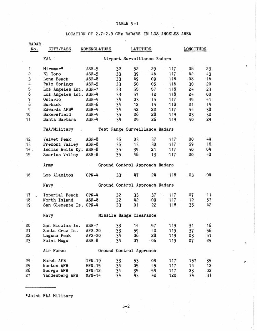
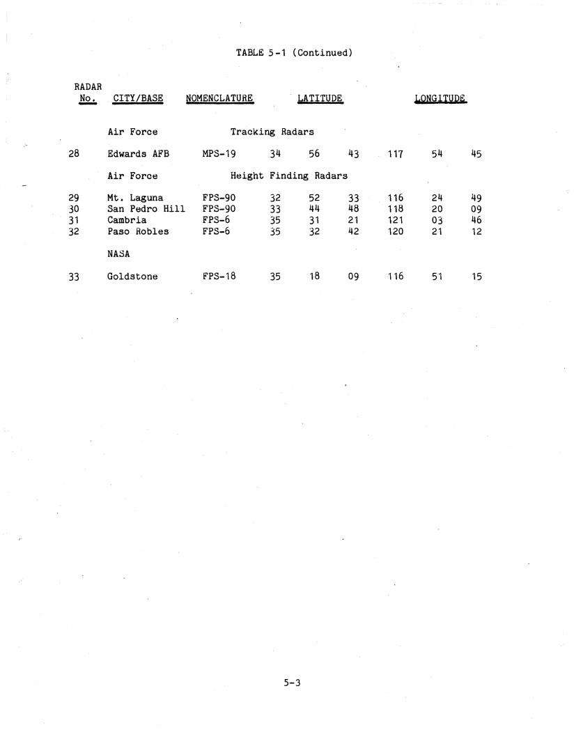
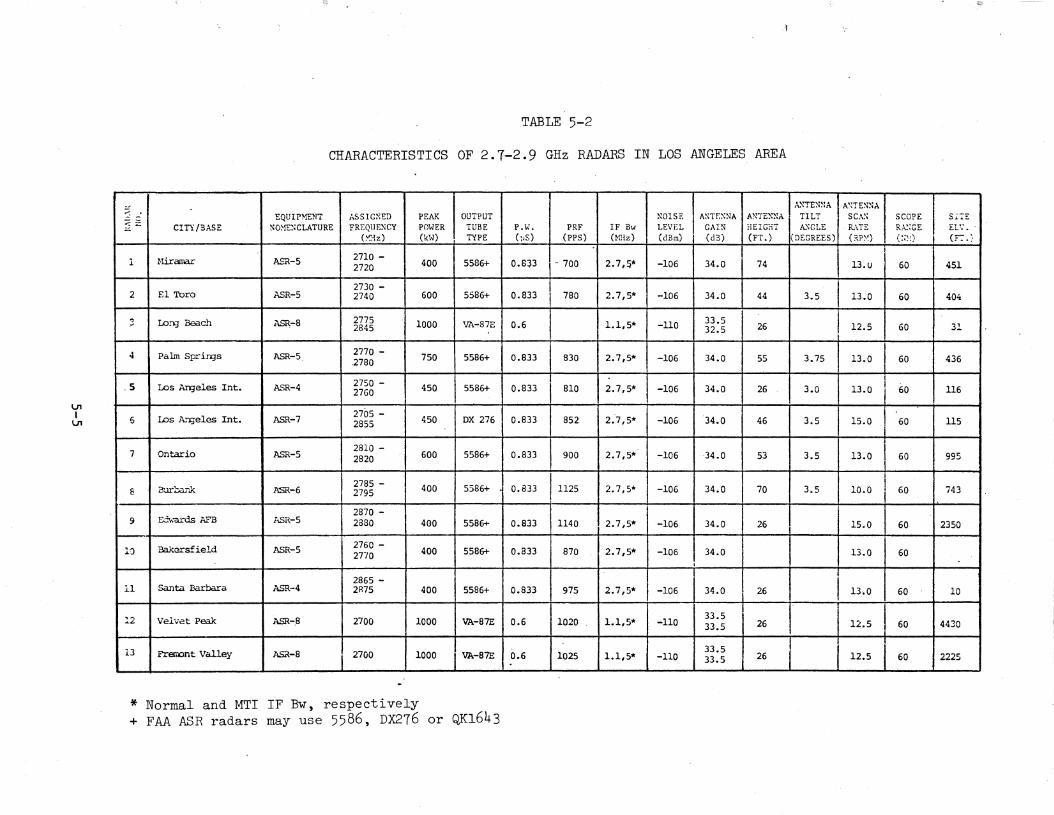
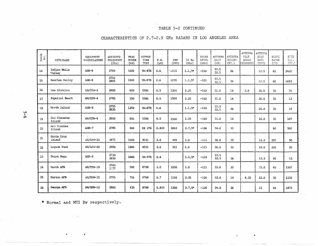
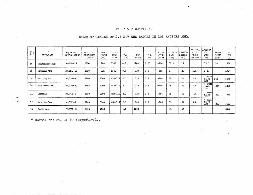
The present radar environment for the Los Angeles area was determinedusing information obtained from the Western Region FAA Frequency Manager, andthe Government Master File. Comparison was made between these two sources, anddifferences resolved by contacting the FAA and DoD area frequency coordinators.It was determined that there are a total of 33 radars within the Los Angelesarea operating in the 2.7 to 2.9 GHz band. TABLE 5-1 lists the location,nomenclature and function of these radars. Figure 5;-1 shows the location ofthese radars on a Los Angeles area map. The equipment characteristics of theradars are given in TABLE 5-2. .
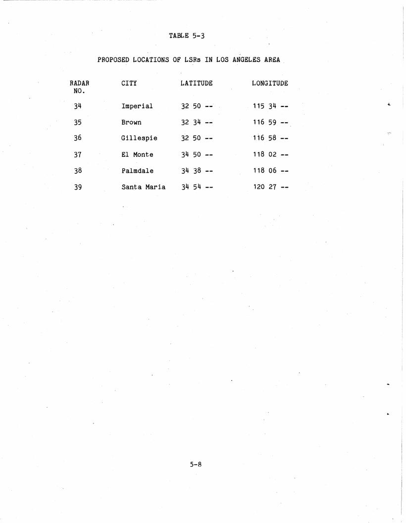
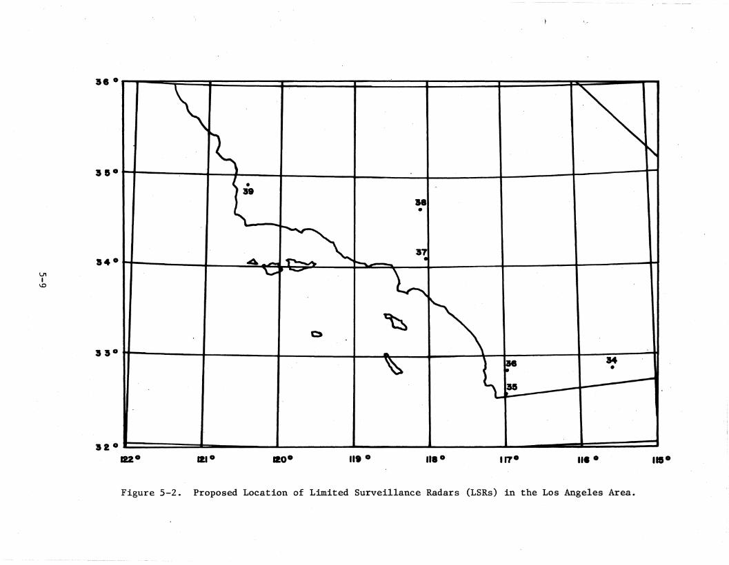
Six potential Limited Surveillance Radar (LSR) sites have been identifiedin the Los Angeles area. TABLE 5-3 shows the approximate Latitude/Longitudallocations for the LSR sites, and Figure 5-2' shows the location of the LSRradars in the Los Angeles area.
~H Q&f~QXMEHT
-The following is a discussion of the feasibility of deploying LSRs at thesix proposed sites in the Los Angeles area (see TABLE 5-3 and Figure 5-2)without degrading the performance of existing radars in the environment, or theLSR radars .
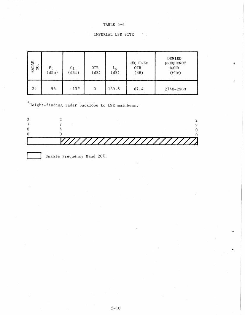
. Im~erial b~R
There is only one potential interfering radar to the Imperial LSR. TheMt. Laguna AN/FPS-90 radar (Radar No. 29) could potentially cause performancedegradation to the LSR no matter what frequency it is assigned in the 2.7 to2.9 GHz band when the height-finding radar is nodding at the Imperial LSRbearing. This is because the Mt. Laguna AN/FPS-90 radar is line-of-sight withthe- proposed Imperial LSR. For LSR antenna mainbeam coupling to theheight-finding radar antenna backlobe, approximately 20 percent of the band canbe used for operation of the Imperial LSR. TABLE "5-4 shows the usablefrequencies for the LSR operation.
5-1
TABLE 5-1
, LOCATION OF 2.7-2.9GHz RADARS IN LOS ANGELES AREA
RADARNo. CITY/BASE NOMENCLATURE LATITUDE LONGITUDE- SiLiil8Z iIii$iW
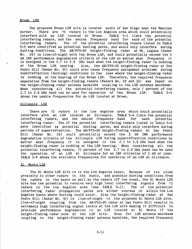
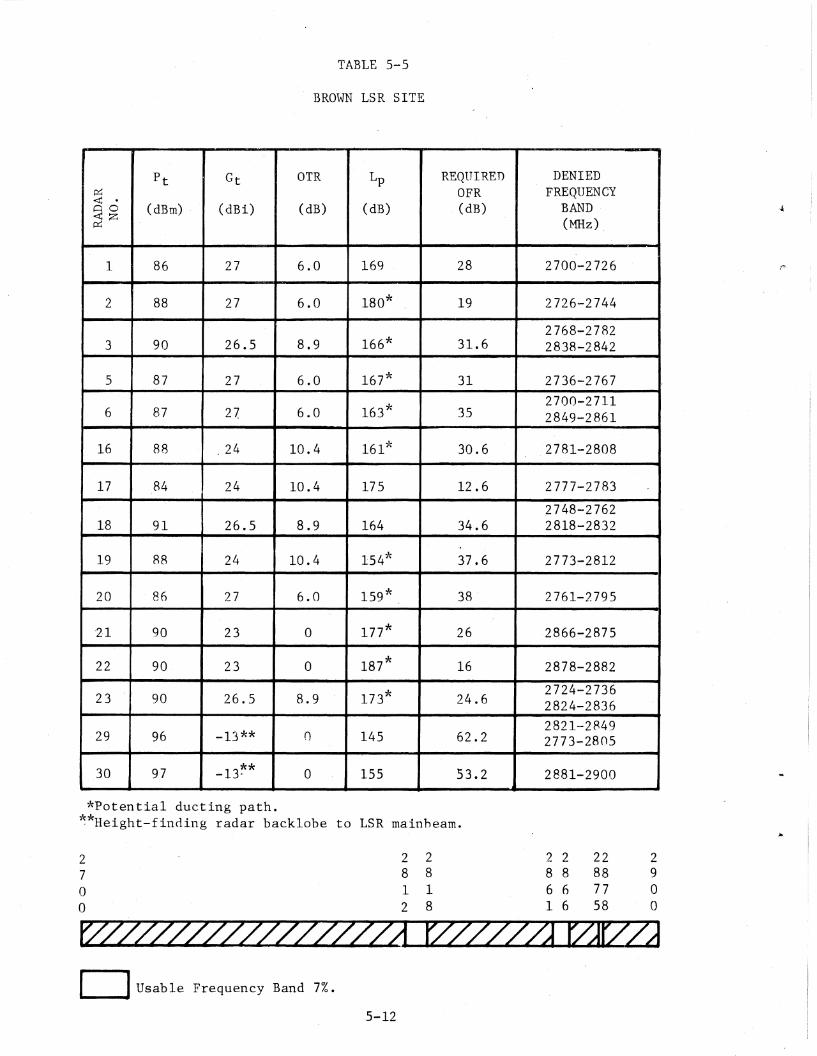
The proposed Brown LSR site is located south ot San Diego near the Mexicanborder. There are 15' radars in the Los Angeles area which could potentiallyinterfere with an LSR located at Brown. TABLE 5-5 lists the potentialinterfering radars, and the denied frequency band for each of the potentialinterfering ,radars. Ten of the potential interfering radars listed in TABLE5-5 were ,identified as potential ductingpaths, and would only interfere duringducting conditions. The AN/FPS-90 height-finding radar at Mt. Laguna (Rad~r
No. 29) is'line-of-sight with the Brown LSR, and could potentially exceed the 5dB INR performance degradation criteria of the LSR no matter what frequency itis as~igned in the 2.7 to 2.9 GHz band when the height-finding r~dar is noddingat the Brown LSR bearing. Also, 'the AN/FPS-90 height-finding radar at SanPedro Hill (Radar No. 30) could also cause frequency assignment problems duringsuperrefraction (ducting) conditions in the case where the height-finding radaris nodding at the bearing of the Brown LSR. Therefore, the required frequencyseparation from the height-finding radars (Radars No. 29 and 30) was based onthe height-finding radar antenna backlobe coupling to the LSR antenna mainbeam.When considering all the potential interfering radars, only 7 percent of the2.1 to 2.9 GHz band can be used for operation of the Brown LSR. TABLE' 5-5shows the usable frequencies for an LSR located at Brown.
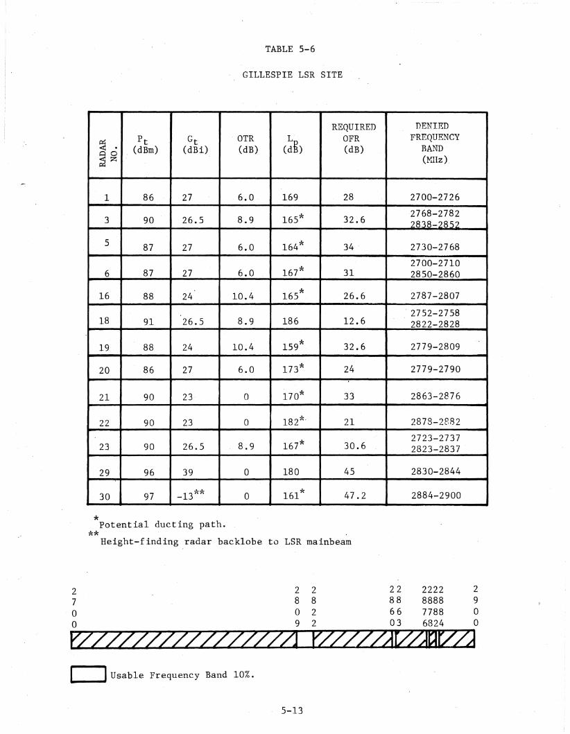
There are 13 radars in the Los Angeles area which could potentiallyinterfere w~th an LSR located at Gillespie. TABLE 5-6 lists the potentialinterfering radars, and the denied frequency band for each potentialinterfering radar. Te~ of the potential interfering radars listed in Table 5-6were identified as potential ducting paths, and would only interfere duringperiods of superrefraction. The AN/FPS-90 height-finding radars at San PedroHill (Radar No. 29) could potentially exceed 'the 5 dB INR performancedegradation criteria of the Gillespie LSR during superrefraction conditions nomatter what frequency it is assigned in the 2.'7 to 2.9 GHz band when theheight-finding radar is nodding at the LSR bearing. When considering all thepotential interfering radars, 10 percent of the 2.7 to 2.9 GHz band can be usedfor operation of an LSR at Gillespie for an INR criterion of 5 dB or less.TABLE 5-6 shows the available frequencies for operation of an LSR at Gillespie.
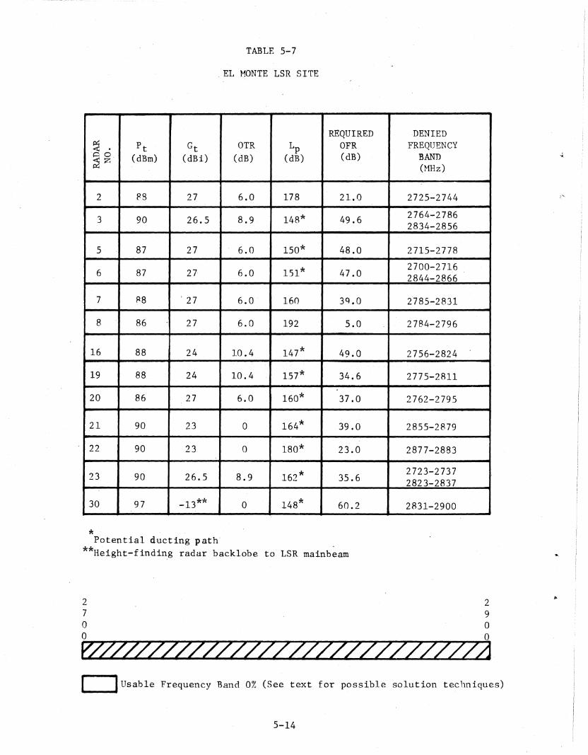
The El Monte LSR site is in the Los Angel~3s basin. Because of its closeproximity to other radars in the, basin, and possible ducting conditions fromthe radars in the basin as well as the radars off the coast, the"EI Monte LSRsite has the potential to receive very high level interfering signals from 13radars in the Los' Angeles area (see TABLE 5-(7). Ten of the potentialinterfering radar propagation paths are e:ither oversea or within the LosAngeles basin where ducting could occur. Also the height-finding radar at SanPedro Hill (Radar No. 30) is line-of-sight to the propo~~d El Monte LSR site.Line-of-sight coupling from the AN/FPS-90radar at San Pedro Hill results inextremely high interfering signal levels at the LSR site making it difficult topreclude performance degradation to an LSR located at El Monte if theheight-finding radar nods at the LSR site. Even for LSR antenna mainbeamcoupling to the height-finding radar antenna backlobe, ·the required frequency
5-11
TABLE 5-5
BROWt-l LSR SITE
Pt Gt OTR Lp REQUIRED DENIED~ OFR FREQlJENCY~
~o (dBm) (dBi) (dB) (dB) (dB) BAND~Z (MHz)
1 86 27 6.0 169 28 2700-2726
2 88 27 6.0 180* 19 2726-2744
2768-27823 90 26.5 8.9 166* 31.6 2838-2842
5 87 27 6.0 167* 31 2736-2767
163 1<2700-2711
6 87 2l 6eO 35 2849-2861
16 88 .24 10.4 161;'< 30.6 2781-2808
17 84 24 10.4 175 12.6 2777-2783
2748-276218 91 26.5 8.9 164 34.6 2818-2832
19 88 24 10.4 154* 37.6 2773-2812
20 86 27 6.0 159* 38 2761-2795
21 90 23 0 177* 26 2866-2875
22 90 23 0 187* 16 2878-2882
23 90 26.5 8.9 173* 24.62724-27362824-2836
-13**2821-2849
29 96 0 145 62.2 2773-2805
30 97 -13~* 0 155 53.2 2881-2900
*Potential ducting path.~*Height-finding radar back10be to LSR mainheam.
**H · h f· d· radar back10be to LSR mainbeam. elg t- lnln,g
2 27 9o 0o 0
VZ7T/Tff/7L7L77ZL7/ZZZZZT/ZT/2o Usable Frequency Band 0% (See text for possible solution techniques)
5-14
separation from the height-finding radar denies an LSR deployed at El Monte theuse of approximately 35 percent of the 2.7 to 2D9 GHz band.
Using the procedure given in Section 11 for determining the requiredfrequency separation from radars in the environment, there are no availablefrequency assignments for the El Monte LSR. However, this does not mean thatan LSR cannot be deployed at the El Monte .airport without performancedegradation to the radar system. It may be necessary to use a waveguide filterin one or two of the existing radars, or some t~rpe of signal processingtechnique to suppress interfering signals. (See report 'by Hinkle, ' Pratt andLevy (1979) on radar signal processing.) The least expensive way to remedy thefrequency assignment problem may be to use a waveguide filter in the LosAngeles ASR-4 radar similar to the waVeguide filter used in the AN/GPN-20radar. With a waveguide filter, the denied frequency band caused by the LosAngeles ASR-4 radar could be reduced from 2715-2718 MHz to 2738-2'772 MHz. Thiswould permit the operation of an LSR at El Monte in the 2116 to 2123 MHz band.
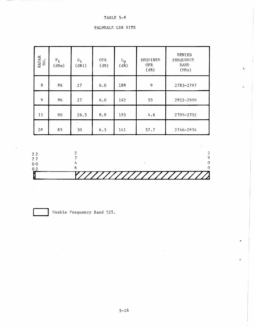
The Palmdale LSR site is located North of the San Gabriel Mountain rangewhich isolates the LSR site from the numerous radars in the Los Angeles basin.There are four potential interfering radars in the Los Angeles area which couldcause degradation to the performance of an LSR located at Palmdale. TABLE 5-8lists the potential interfering radars, and the denied fr~quency band for eachof the potential interfering radars. Approximately 22 percent of the band isavailable for frequency assignment to an LSR located at Palmdale.
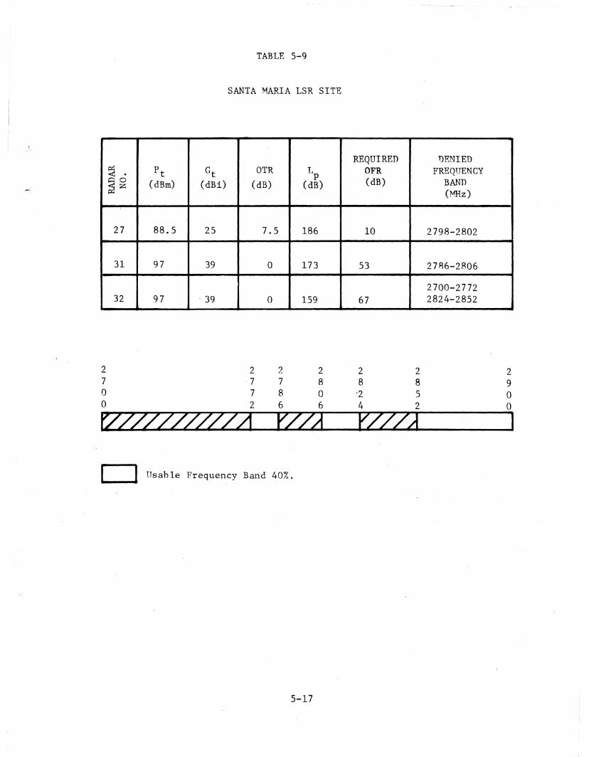
The Santa Maria LSR site is located between the San Rafael mountain rangeand the Pacific Ocean in the Santa Maria Valley.' The Santa Maria LSR site isisolated from most of the Los Angeles area 2.7 to 2.9 GHz radars. There areonly three potential interfering radars which could cause degradation to theperformance of an LSR located at Santa Maria (See TABL~ 5-9). Approximately 40percent of the band is available for frequency assignment to an LSR located atSanta Maria.
5-15
TABLE 5-8
PALMDALE LSR SITE
~DENIED
<1j . P t Gt OTR Lp REQUIRED FREQUENCYc;o~Z (dBm) (dBi) (dB) (dB) OFR BAND
(dB) (~1Hz)
8 86 27 6.0 188 9 2783-2797
9 R6 27 6.0 142 5.5 2822-2900
13 90 26.5 8.9 193 4.6 2700-2702
2R 85 30 6.3 141 57.7 2746-2R34
2 2 2 27 7 7 900 4 002 6 0
~..........-....-.... fZL/7/L727ZZZZ7ZZZZ-LZJ
o Usable Frequency Band 22%.
5-16
TABLE 5-9
SANTA MARIA LSR SITE
REQUIRED DENIED~ P t Gt OTR 1-1 OFR FREQ1JENCY< P~o (dBm) (dBi) (dB) (dB) (dB) BAND~z
This section discusses the feasibility of deploying the LimitedSurveillance Radar (LSR) at eight proposed sites in th-a San Francisco area inthe 2.7 to 2.9 GHz band. The LSR system characteristics and
~ Interference-to-Noise Ratio (INR) criterion used in the investigation arediscussed in Section 3. The procedure used to identify frequencies in the 2.7t9 2.9 GHz band at which the LSR can operate without performance degradation tothe radars presently in the environment, or the LSR, is discussed in Section 4.
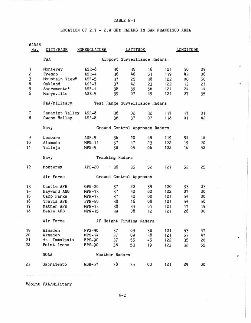
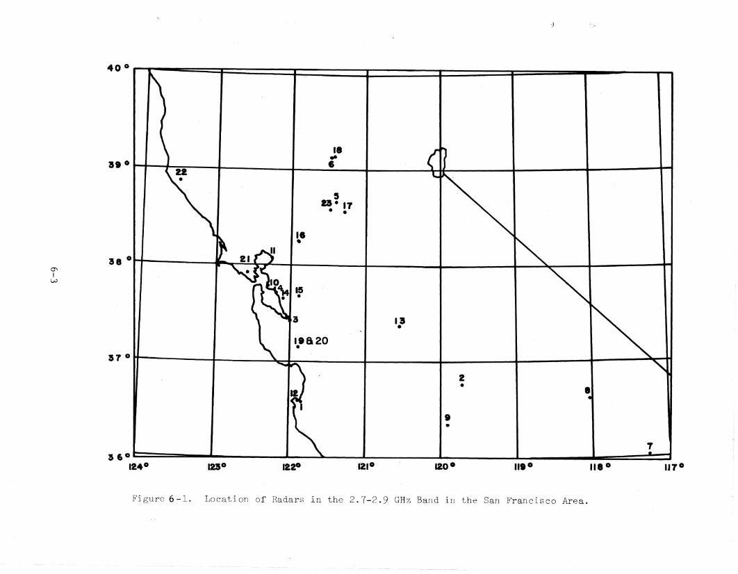
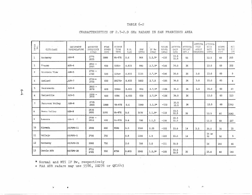
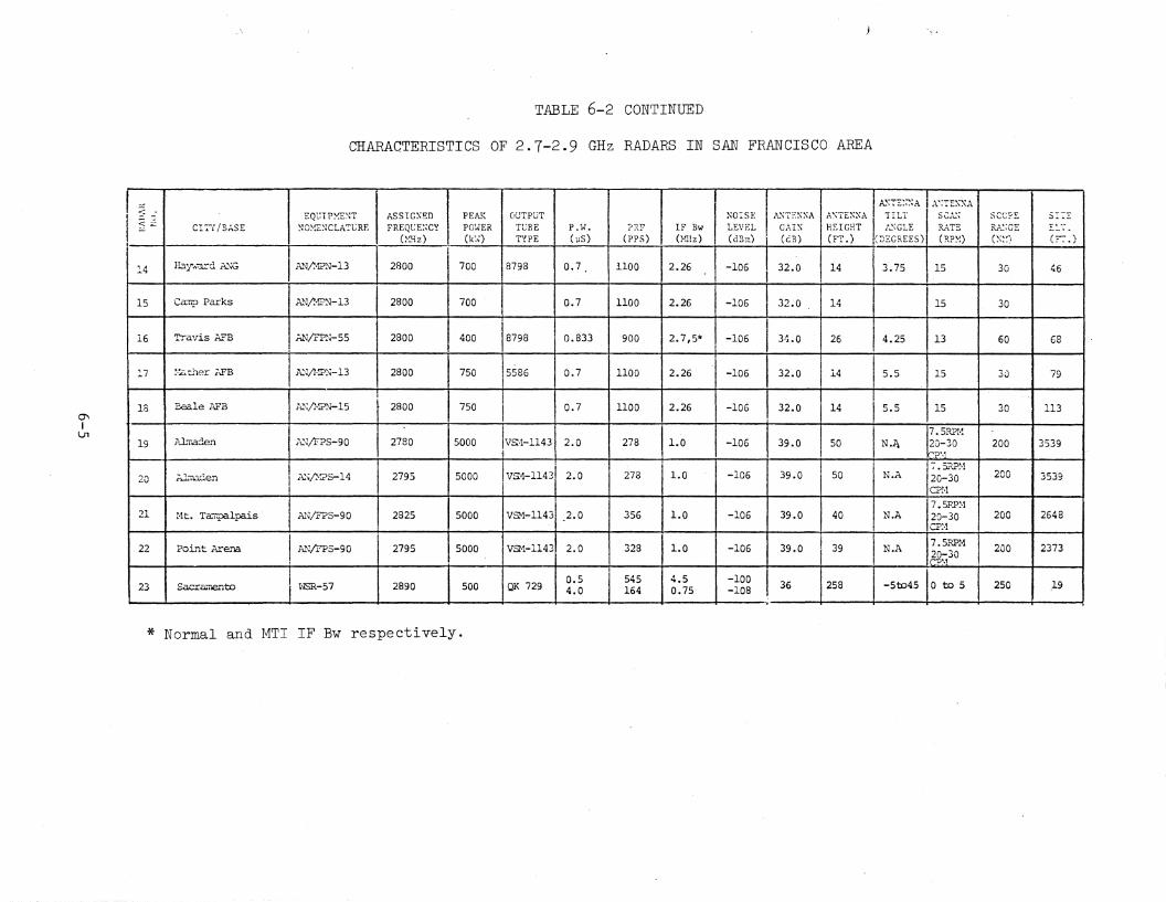
The present radar environment for the San Francisco area was determinedusing information obtained from the Western Region FAA Frequency Manager, andthe Government Master File. Comparison was made between the two sources, anddifferences resolved by contacting the FAA and DoD area frequency coordinators.It was determined that there are 23 radars in the San Francisco area operatingin the 2.7 to 2.9 GHz band. TABLE 6-1 lists the location, nomenclature, andfunction of these radars. Figure 6-1 shows the location of these radars on aSan Francisco area map. The equipment characteristics of the radars are ~iven
"in TABLE 6-2.
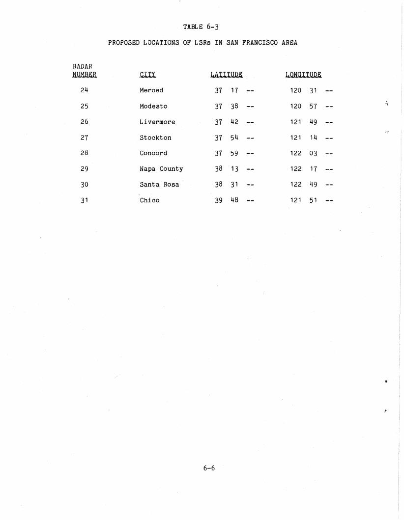
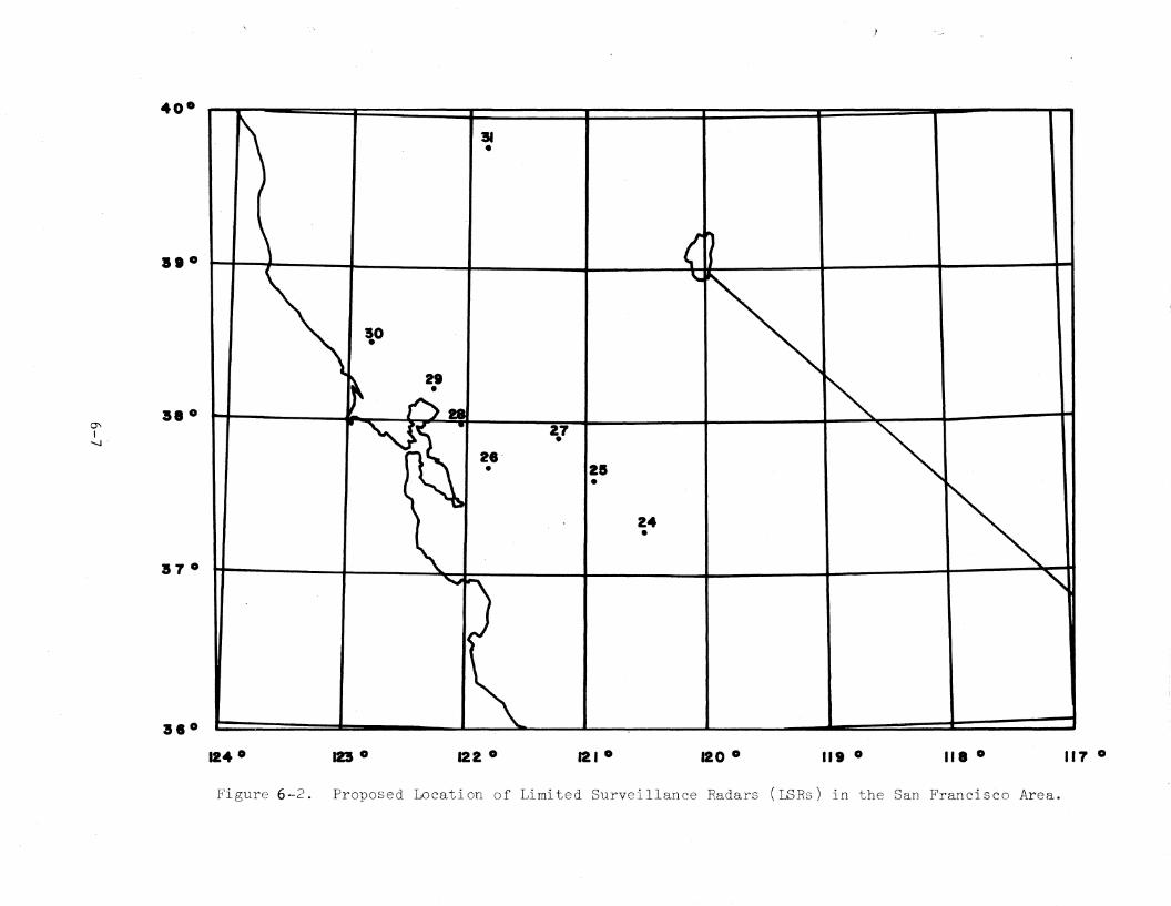
Eight potential LSR sites have been identified in the San Francisco area.TABLE 6-3 shows the approximate latitude/longitude locations for the LSR sites,and Figure 6-2 shows the location of the LSR' radars in the San Francisco area.
The following is a discussion of the feasibility of deploying LSRs at theeight prop9sed sites in the San Francisco area (see TABLE 6-3 and Figure 6-2)without degrading the performance of existing radars in the environment, or theLSR radars.
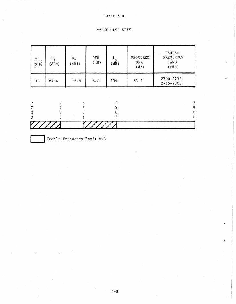
The proposed Merced LSR site is located in the San Joaquin Valley. Thereis only one potential interfering radar to the Merced LSR. The Castle AFBAN/GPN-20 (Radar No. 13) is located approximately 6.7 miles from the proposedMerced LSR site. The Castle AFB radionavigation radar normally operates in thefrequency divers~ty mode at 2715 and 2785 MHz. TABLE 6-4 shows the frequencybands denied by the Castle AFB AN/GPN-20 radar for operation of an LSR atMerced. Approximately 60 percent of the band can be used for operation of theMerced LSR.
6-1
TABLE 6-1
LOCATION OF 2.7 - 2.9 GHz RADARS IN SAN FRANCISCO AREA
3 6 0 r , I '" I I I , • 11240 1U0 1220 1210 120 0 111 0 118 ° 117 0
a. 0 t-t 1 II•• I ~• I , U. I I ~
40 0 rt:--==~if I I I I I I I
(j\
Iw
Figure 6-1. Location of Radars in the 2.1-2.9 GHz Band in the San Francisco Area.
TABLE 6-2
CHARACTERISTICS OF 2.7-2.9 GHz RADARS IN SAN FRANCISCO AREA
l....~TE~\~iA IA'::E;-;:~A
~ :: r:QtIPXEST ASSIG~;ED PEftul( OUTPUT ~OlSE t\.~TE~~A N\TE~;NA TILT SC~\:'i SCOPE S:::;: z: I CITi /3.;5ElKO~!E~CLATuRE I FREQUE~CY PQl,ER TU3 E P •" • PRF IF Bw LEVEL GAlli !lEI CHT 0:GLE RX,E I R.~~ C; E I --..
22 Point Arena IA..'l/FPS-90 2795 5000 VSH-1143 2.0 328 1.0 -106 39.0 I 39 N.A 7.5RPM
I 200 2373t I ~~30
~ ~·1
~1SR-57 2890 500 QK 7290.5 545 4.5 -100 I 36 258 -5to45 10 to 5 250 1923 Sacra..uento 4,,0 164 0,,75 -108 I ,
'f
* Normal and MTI IF Bw respectively.
TABLE 6-3
PROPOSED LOCATIONS OF LSRs IN SAN FRANCISCO AREA
RADARNUM6~H .c.uI r..AllIUU~ LQNGITUDE
24 Merced 31 1'7 120 31
25 Modesto 31 38 120 57 "'\
26 Livermore 31 42 121 49
27 Stockton 31 54 121 14
28 Concord 31 59 122 03
29 Napa County 38 13 122 11
30 Santa Rosa 38 31 122 49
31 Chico 39 48 121 51
6-6
40·
at O
38 0 II r~l ·'2. 27•~
II
'-J .
25•
24•
II I , I. Ia7°
al O
124 0 123 0 122 0 121 0 120 0 II' 0 118 0 117 0
Figure 6~2. Proposed Location of Limited Surveillance Radars (LSRs) in the San Francisco Area.
TABLE 6-4
MERCED LSR SIrE
DENIED
~ Pt
Gt
OTR L REQUIRED FREQUENCY~ P~o (dBm) (dBi) (rlB) (dB) OFR BAND5 Z (dB) (1vlliz)p::;
13 87.4 26.5 6.0 1.34 63.9 2700-27352765-2805
-
29oo
27.35
27oo
2 27 86 05 5
fZ27ZJ---rz/7JZa~ ]o Usable Frequency Band: 60%
6-8
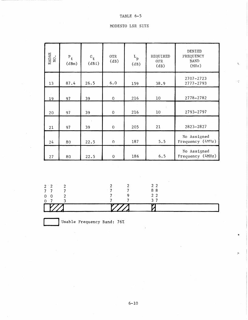
Modesto LS.R
There are six radars in the San Francisco area which could potentiallyinterfere with an LSR located at Modesto. TABLE 6-5 lists the potentialinterfering radars, and the denied frequency band of each potential interferingradar. The height-finding radars (Radars Nos. 19 and 20) will only interferewith the LSR when they are nodding at the bearing of the Modesto LSR. TABLE6-5 shows that approximately 16 percent of the band is available for operationof an LSR at Modesto.
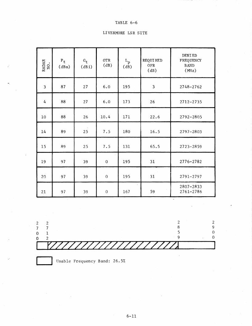
Li ver:.Iqore _ LSI!
The proposed Livermore LSR site is located in the Livermore Valley east ofthe San Francisco Bay. Livermore Valley has mountain ranges or hills on allfour sides. There are eight radars in the San Francisco area which couldpotentially interfere with an LSR located at Livermore. TABLE 6-6 lists thepotential interfering radars, and the denied frequency band for each potentialinterfering radar. When considering all the potential interfering radars, 26.5percent of the 2.1 to 2.9 GHz band can be used for operation of an LSR atLivermore.
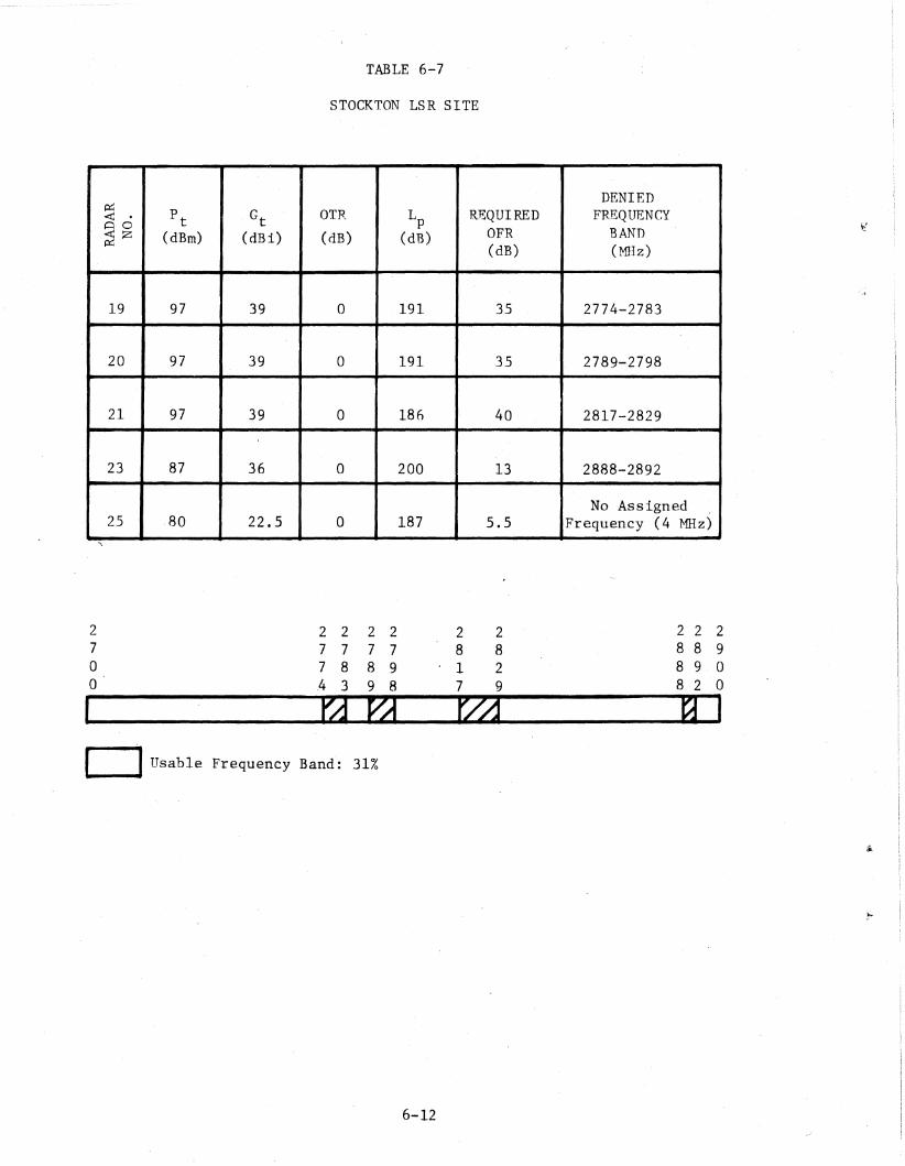
The proposed Stockton LSR is located in the San Joaquin Valley. There arefive radars which could potentially interfere with an LSR located at Stockton(see TABLE 6-7). Three of the potential interfering radars are height-f~nding
radars located at Almaden (Radars Nos. 19 and 20) and Mt. Tamalpais (Radar No.21). The other two potential interfering radars are the Sacramento weatherradar (Radar No. 23), and a proposed LSR at Modesto (Radar No. 25). TABLE 6- 17shows the denied frequency band for each of the potential interfering radars.Approximately 81 percent of the band is available for frequency assignment toan LSR located at Stockton.
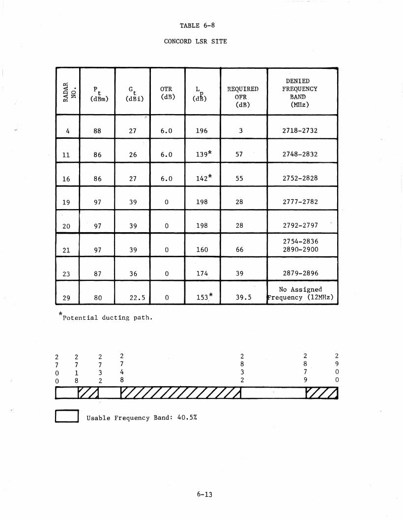
QODCOtQ bSfi
Eight radars in the San Francisco area were identified as potentialinterfering radars if an LSR is located at Concord (see TABLE 6-8). Two of thepotential interfering radar propagation paths (Vallejo AN/MPN-5 and Travis AFBAN/FPN-55) were identified as possible ducting paths. Also, the path betweenthe proposed Napa County LSR and the Concord LSR was identified as a possibleducting path. Three height-finding radars (Radar Nos. 19, 20, and 21) couldalso potentially interfere with an LSR located at Concord. When consideringall the potential interfering radars, 40.5 percent of the 2.7 to 2.9 GHz bandcan be used for operation of an LSR at Concord. TABLE 6-8 shows the availablefrequencies for operation of an LSR at Concord.
The Napa County LSR is located at the North end of the San Francisco/SanPablo Bay. Because the proposed LSR site is located near the North end of theBay, propagation ducting phenomena, which occurs approximately 50 percent ofthe time in the Bay area, significantly increases the potential of interferenceto the proposed Napa County LSR. There are 12 radars in the San Francisco area
1 fZ1_(ZT/TLZ22ZTr/Lt........-.-.- fZZ1r==:=J Usable Frequency Band: 40.5%
6-13
which could potentially interfere with an LSR located at the Napa CountyAirport. TABLE 6-9 lists the potential interfering radars, and the deniedfrequency band for each potential interfering radar. Five of the potentialinterfering radar propagation paths were identified as potential ducting paths.The Mt. Tamalpais height-finding radar (Radar No. 21) is line-of-sight with theproposed LSR site, and denies the LSR located at Napa County Airportapproximately 79.5 per.cent of the band even for LSR antenna mainbeam couplingto th~ height-finding radar antenna backlobe.
Using the procedure given in Section 4 for determining the requiredfrequency separation from radars in the environment, there are no availablefrequency assignments for the Napa County LSR. However, this does not meanthat an LSRcannot be deployed at the Napa County Airport without performancedegradation to the radar system. A worst case measured height-finding radaremission spectrum (see Appendix A) was used in this analysis. An accuratemeasurement of the Mt . Tamalpais radar emission spectrum may show that the l'1t.Tamalpais radar would not deny deployment of an LSR at the Napa County Airport.Also, if necessary, a waveguide filter could be used in the Mt. Tamalpais radarwhich would permit deployment of an LSR at the Napa County Airport.
There are nine radars in the San Francisco area which could potentiallyinterfere with an LSR located at Santa Rosa. TABLE 6-10 lists the potentialinterfering- radars, and the denied frequency band for each of the potentialinterfering.radars. Six of the potential interfering radar propagation pathswere identified as possibleducting paths. Four height-finding radars (RadarNos. 19 through 22) were identified as posible interfering radars. It isdifficult to preclude degradation in the Santa Rosa LSR if the height-findingradars at Almaden and Mt. Tamalpais nod at the bearing of the LSR. Whenconsidering all potential interfering radars, 33 percent of the 2.7 to 2.9 GHzband can be used for operation of anLSR at Santa Rosa. TABL~E 6-10 shows theavailable frequencies for operation of an LSR at Santa Rosa.
There are no rada~s in the 2.7 to 2.9 GHz band within 50 statute miles ofthe proposed LSR site at Chico. Therefore, 100 percent of the band isavailable for freq.~uency assignment of an LSR at Chico.
6-14
TABLE 6-9
NAPA COIJNTY LSR SITE
DENIED~
P t Gt OTR Lp REQUIRED FREQUENCY< .~o
~z (<iBm) (dBi) (dB) (dB) OFR BAND(MHz)
3 87 27 6.0 162* 36 2728-2769
4 88 27 6.0 146* 53 2700-2754
10 88 26 10.4 145* 48.6 2758-2822
11 86 26 6.0 134* 62 2734-2846
14 89 25 7.5 161* 35.5 2778-2809
15 89 25 7.5 190 6.5 2798-2802
16 86 27 6.0 184 12 2798-2802
19 97 39 0 184 42. 2771-2784
20 97 39 0 184 42 2786-2799
21 97 -13** 0 134 . 74.5 2741-2900
23 87 36 0 208 5 2R88-2892
28 80 22.5 0 153 39.5No Assigned
Frequency (12MHz)
*Potential ducting path*,te .Height-finding radar back10be to LSR mainbeam
2 2 27 8 9o 0 0o 0 0
PZffa77/T§T//2ZTmzr///ZT~o Usable Frequency Band: 0% (See text for possible solution techniques)
6-15
29oo
TABLE 6-10
SANTA ROSA LSR SITE
~DENIED
<C . Pt
Gt
OTR L REQUIRED FREQUENCY00~Z P
(dBm) (dBi) (dB) (dB)OFR BAND(dB)_ (Mllz)
3 87 27 6.0 157* 41 2724-2772
4 88 27 6.0 152''( 47 2700-2747
10 88 26 10.4 152* 41.6 2769-2815
11 86 26 6.0 189 7 2798-2802
14 89 25 7.5 151* 45.5 2769-2815
-13** * 2764-278819 97 0 151 57.5
20 97 -13** 0 151* 57.5 2799-2803
2807-283421 97 -13** 0 147 61.5 2759-2789
22 97 39 0 200 26 2792-2797
*Potentia"1 ducting path.
**Height-finding radar back10be to LSR mainbeam
2 27 8o 3o 4
~47/7//ZT§/Z/j........~ ____o Usable Frequency Band: 33%
6--16
APPENDIX A
FREQUENCY-DEPENDENT-REJECTION
The Frequency-Dependent-Rejection (FDR) model accounts for the energycoupling loss of an undesired signal in a victim receiver due to Off-FrequencyRejection (OFR) and On-Tune Rejection (OTR) of the undesired signal, and istherefore a necessary component in predicting radar-to-radar interferencelevels. The factors which affect the FDR of a victim radar are the victimreceiver IF selectivity characteristics, undesired signal emission spectrum,and the frequency separation between the interfering and victim radars. Thisappendix discusses techniques used to compute the FDR factor. FDR curves usedin determining the feasibility of deploying the LSR in the Los Angeles and SanFrancisoo areas are also presented.
Sinoe the victim receiver frequency selectivity is the principal means bywhich thereoeiver discriminates against undesi.red signals, it is an importantinput parameter to the FDR model. Receiver spurious responses must also beconsidered when determining the FDR of a victim radar to an undesired signal.Spurious responses occur when the undesired signal is at a frequency such thatit mixes with the local oscillator to produce an output at the receiver IFfrequenoy. Sinoe most radars have preselector filters, only image responseswere investigated. The local oscillator frequency of most radars in the2.7-2.9 GHz band are tuned to 30 MHz above the receiver RF tuned frequencies inorder to obtain an IF frequency of 30 MHz. An RF undesired signal that is 30MHz above the local oscillator frequency (60 MHz above RF receiver center tunedfrequency) will also be down-converted to the 30 MHz IF frequency. Modernradars normally employ an image-rejection mixer or a·notch filter at the radarinput to suppress image responses. Based on previous radar measurements, theimage response of the LSR should be at least 50 dB down. Reduced FDR due toreceiver image response was not incorporated in the FDR model, but wasconsidered in an independent FDR calculation.
The'selectivity of a receiver is the composite selectivity of all tunedcircuitry in the receiver prior to detection; however, in a super~eterodyne
receiver, the selectivity is determined by the IF stages because the precedingmixer and RF circuits 'are relatively broader band. This is because therequired' filter characteristics are more physically realizable and lessexpensive to build at the lower IF frequency.
Since the LSR is in the field evaluation stage, and specifications havenot been finalized, the number of IF stages and IF selectivity characteristicsare not known. Only the 3 dB IF selectivity bandwidth of the LSR was given onthe OT-34 form. The specified 3 dB IF selectivi.ty was 600 kHz. Since mostradars in the 2.7-2.9 GHz band have at least five tuned stages, a five-tuned
A-I
stage IF selectivity model was used with a 600 kHz bandwidth to represent theIF selectivity characteristics of an LSR. Figure A~1 shows the modeled IFselectivity characteristics used in determining theFrequency-Dependent-Rejection (FOR) of an LSR to undesired signals.
The emission spectrum of a pulse radar is determined by the modulatingpulse shape and width, transmitter RF tube, and RF output tube load. Thetrartsmission waveguide, rotary couplers, and antennas also affect the emissionspectra but to a much less degree. The emission spectrum of radars in the2.7-2.9 GHzband were categorized according to their pulse width, transmitterRF tube, and whether or not the radar used a waveguide filter. TABLE A-1 showsthe categorization of the radars by nomenclature.
The emission spectra of radars in categories 1 through 4 were obtainedusing a model by Newhouse (1969) which takes into account the frequency shiftcharacteristics of the conventional magnetron. The model was validated bymeasurements made with the Radio Spectrum Measurement System (RSMS) van. Bothmodeled and measured emission spectra for the four categories are given in areport by Hinkle, Pratt and Matheson (1976). The modeled emission spectra forcategories 1 through 4 are shown in Figures A-2 through A-5 respectively. Theemission spectra of radars in categories 5 through 7 were obtained using theRSMS van measurement capability. The measured emission spectra were used inthe FDR model for categories 5 through 1. Figures A-6 through A-8 show themeasured emission spectra of the radars in categories 5 through 7.
Several emission spectrum measurements of height-finding radars (Category7) were made using the RSMS van. The height-finding radars (AN/FPS-6, 90) usea coaxial magnetron RF output tube. The undesired mode shown in Figure A-8 onthe upper-side of the fundamental frequency was observed on all height-findingradars using a coaxial magnetron. However, the undesired mode shown in figureA-8 on thelower~side was not observed on all the height-finding radar measuredemission spectra. These undesirable coaxial magnetron modes are caused byimproper rise and fall time of the modulating pulse, and inadequate modesuppression in the coaxial magnetron tube.
Present plans are to use a Traveling-Wave Tube (TWT) RF output tube in theLSRs. A modeled emission spectrum for a trapezoidal pulse shape was used forthe LSR. Figure A-9 shows the modeled LSR emission spectrum for a 2.0 ps pulse~idth and 0.2 ps rise time. The ris~ time was based on an expected 0.1 pulsewidth range accuracy (FAA,·1~78).
FaR CA~CU~AIIQNS
Frequency-Dependent-Rejection (FOR) is the sum ofundesired signal due to Off-Frequency-RejectionOn-Tuned-Rejection (OTR) in dB.
T = Interfering transmitter pulse width,in seconds
A computer program based on CCIR Report 654 was used to obtain the OFRfactor. Inputs to the program consisted of amplitude (dB) and frequency datapoint pairs of the undesired, signal emission spectrum and victim re~eiver IFselectivity curves. The computed OFR curves used for determining the OFR of anLSR to the various categories of radar emission spectrums (See TABLE A-1) areshown in Figures A-10 through A-17.
This appendix contains an analysis of the signal processing ofasynchronous pulsed interference through the LSR receiver, and appropriateperformance criteria for the LSR, in a asynchronous pulsed interferenceenvironment. An appropriate peak lnterference-to-Noise Ratio (INR) to precludeperformanoe degradation to the LSR 1s developed. This peak INR criterion wasthen used to assess the feasibility of deploying LSRs in the 2.7 to 2.9 GHzband in the Los Angeles 'and San Francisco areas.
PERFORMANCE CRITERIA
In order to assess the feasibility on an electromagnetic capability (EMC)basis of deploying the LSD radars in the Los Angeles and San Francisco area, itis necessary to establish a peak Interference-to-Noise Ratio (INR) ,which willpreqlude performance degradation of the LSR System. For this investigation,the criteria used to establish an appropriate peak INR was:
1.' The level of interference should not cause false hit reports'to be sent to the MTD PO,st-processor which could resul t inoverloading of the post-processor.
2. The level of interference should not ,cause the MTD threshhold level to be increased by more than 1 dB.
It is shown in a report by Hinkle, Pratt and Levy (1979) that the peakInterferenoe-to-Noise Ratio (INR) gain through a phase detector and a low passfilter when matched to one~half the receiver IF bandwidth and averaged over allphase angles is 0 dB. Therefore, the peak INR at the receiver IF output isequal to the peak INR at the MTD processor input (A/D converters).
To analyze the effects of asynchronous pulsed interference on the MTDprocessor, both the canceller/transversal filter channel and the Zero VelocityFilter (ZVF) channel,signal processing must be considered. The following is acursory analysis of the signal processing of both channels for noise andasychronous pulsed interference.
Canceller/Transversal Filter Channel
The MTD-II radar at Burlington, Vermont has a two-pulse canceller prior tothe seven t~ansversal filters, sometimes called Finite Impulse Response (FIR)filters. Consideration is being given to not using a MT! canceller _prior tothe FIR filters in the LSR. Because of the uncertainty in whether or not aoanceller will be used in the LSR, the transfer properties of the MTD-II withand without a canceller for both noise and asynchronous pulsed interferencewill be disoussed. As previously mentioned, tne number of doppler filtersproposed for the LSR is 16. However, it may be decided later that only eightdoppler filters will be used. Also ,the type of FIR filters (recursive ornonrecursive), or filter coefficients (weights) to be used in the LSR are not
B-1
known. Therefore, for this analysis the FIR filter characteristics in theMTD-II will be used to determine a peak INR criterion to be used for the LSR.
Canceller
The following is a discussion of the transfer properties of a two-pulsecanceller to noise and asynchronous pulsed interference.
Noise. Since the RMS noise is uncorrelated from epoch to epoch, the RMSnoise voltage gain of a canceller can be expressed as:
where:
=j~i=O
a?1
(B-1)
Binominal weighting factors, (_1)i(~)
m = Canceller filter order, 1 for two-pulsecanceller
Therefore, the noise voltage gains for a two-pulse canceller is equal to ~
Interference. Since the binomial weighting factors for a two-pulsecanceller are 1 and -1, the peak interference voltage gain through a two-pulsecanceller is one. However, the time response of the canceller to asynchronouspulsed interference is important since it has an effect on the gain through theFIR filters which follow. For asynchronous pulsed interference, . eachinterfering pulse at the canceller input will produce several synchronouspulses which will appear at the input of the FIR filter simultaneously. Atwo-pulse canceller will produce two synchronous pulses at the output of thecanceller for each interfering pulse with an amplitude proportional to thebin6minal weighting factors (1 and -1).
Transversal Filter
The MTD-II has seven doppler filters which are implemented using linearphase nonrecursive transversal filter~ (FIR filter~). Since the filters arelinear-phase, the impulse responses or weights of the filters ,are real. TABLEB-1 shows the filter weights, h (n), for each of the seven transversal filtersfor both the 1nphase (I) and Quadrature (Q) channels in the MTD-II. Figure B-1shows a block diagram for a nonrecursive transversal filter (FIR filter).
Noise. Neglecting the noise correlation of the canceller, the RMS noisevoltage gain of a nonrecursive transversal filter can be expressed as:
(B-2)
where:
N = Number of filter samples, 7hen) = Transversal filter weights
B-2
tdIw·
TABLE B-1
TRANSVERSAL FILTER WEIGHTS
FILTER FILTERWEIGHTSh(n) 1 2 3 4 5 6 7
I Q I Q I Q I Q 1 Q I Q I 0
0 -3 -3 2 -3 1 0 1 0 1 0 2 3 -3 3
1 4 . -7 8 6 -2 3 .. -3 0 -2 -3 8 -6 4 7
2 11 5 -12 13 -2 -6 6 0 -2 6 -12 -13 11 -5
3 -2 15 -15 -15 ·7- 3 -7 0 7 -3 -15 15 -2 -15
4 -12 1 15 -12,.
3 6 0 -6 -3 13 12 -12 -1-0
5 -2 -8 6 8 1 -4 -3 0 1 4 6 -8 -2 8
6 4 -2 -3 2 1 1 1 0 1 -1 -3 -2 4 2
x(n) Z-l Z-l Z-lI • • •
Z-l
tdI~
h(O)
y(n)
Figure B-1. Direct Form of Finite Impulse Respon~)e (FIR) Filter
." 1. 1':
The noise voltage gain (nTFG) for each filter for the I and Q channels is shownin TABLES B-2 and B-3.
Interference. The gain of the interference through the transversalfilter is a function of whether or not a cance~ler precedes the transversalfilters. When a two-pulse canceller precedes the FIR filters, there will betwo interfering pulses, on two inputs to the FIR filters simultaneously withnoise on the other five FIR filter inputs. If a canceller is not used, theremost likely will only be one interfering pulse on the inputs to the FIR filtersfor asynchronous pulsed interference with noise on the other six FIR filterinputs.
When a two-pulse canceller precedes the FIR filters, the peak interferencegain of the FIR filters to asynchronous pulsed interference is given by:
i rFc = Ih(n) - h (n-l) I
For: n = 0 to N
(B-3)
The 'peak Interference-to-Noise Ratio (INR) voltage gain through the two pulseoanceller and FIR filters can be expressed as:
INR = Ih(n) - h (n-l) I (B-4)
..r;- .. I N-lV ~. h2 (n)
n=O
For: n = 0 to N
In order to determine the peak Interference~tol-Noise Ratio (INR) at thetransversal filter channel ~utput, Equation B-4 must be iterated for both the Iand Q'channel, and the magnitude algorithm applied. The magnitude of the I andQ channels is obtained by comparing the I and Q signal levels at the'FIR filteroutput~, and applying the following algorith~s.
7/8 LARGER + 1/2 SMALLER (B-5)
This new quantity is compared to LARGER and the greater value transmitted tothe output oircuit.
The peak INR gain through the two-pulse cancellers and FIR filter wascalculated using Equation B-4 for both I and Q channels and applying themagnitude algorithm (Equation B-5). TABLE B-2 shows the maximum peak INR gainthrough the Transversal filter channel for each filter when a two-pulsecanceller is'· used. The maximum peak INR gain through the transversal fil terchannel when a canceller is used is -0.5 dB. It should be noted that the peakINR gains shown in TABLE B-2 are the maximum peak INR gain for each filter.The average peak INR gain for each filter would be a few dB lower.
B-5
OJI0\
TABLE B-2
PEAK INTERFERENCE-TO-NOISE RATIO GAIN FOR TRANSVERSAL FILTER CHANNEL WITH TWO-PULSE CANCELLER
CANCELLER FIR FILTER FIR FILTER FIR FILTER FIR FILTER MAGNITUDE TRANSVERSIALFILTER NOISE NOISE INTERFERENCE OTT'fPlTT OUTPUT OUTPUT FILTERNUMBER VOLTAGE VOLTAGE VOLTAGE INR VOLTAGE INR GAIN INR VOLTAGE CHANNEL
GAIN GAIN GAIN GAIN (dB) GAIN GAIN (dB)
I ,f2 17.72 10 0.399 '" -7990.645 -3.8
1 /2Q 19.41 14 0.510 -5.8
I f2 26.58 30 0.798 -2.02 0.739 -2.6
Q f2 25.51 3 0.083 -21.6
I- ff 9.79 9 0.650 -3.73 0.947 -0.5
Q Iz 8.94 9 0.712 -2.9
I 12 11.87 13 0.774 -2.2 -2.24 0.774
Q 12 0 0 N/A N/A
I 12 9.79 9 .650 -3.75 0.947 -0.5
Q 12 8.94 9 0.712 -2.9
I 12 25.51 3 0.083 -21.66 0.720 -2.8
Q 12 25.51 28 : 0.776 -2.2
I 12 17.72 10 0.399 -7.9-3.87 0.645
Q 12 19.41 14 0.510 -5.8
-,"t "r
tdI
.......
-J
TABLE B-3
PEAK INTERFERENCE-TD-NOISE RATIO GAIN FOR TRANSVERSAL FILTER CHANNEL WITH NO CANCELLER
FIR FILTER FIR FILTER FIR FILTER FIR FILTER MACRITUDE TRANSVERSALFILTER NOISE INTERFERENCE OUTPUT OUTPUT OUTPUT FILTERNUMBER VOLTAGE VOLTAGE INK VOLTAGE INR GAIN INR VOLTAGE CHANNEL
GAIN GAIN GAIN (dB) GAIN GAIN (dB)
I 17.72 2 0.112 ~-19.0
-2.21 0.773
Q 19.41 15 0.773 -2.2
I 26.58 15 0.564 -5.02 0.796 -2.0
Q' 25.51 15 0.588 -4.6
I 9.79 7 0.715 -2.93 0.793' -2.0 ~
Q 8.94 3 0.335 -9.4
1 11.87 7 0.590 -4.6 0.590 -4.64
Q 0 0 N/A N/A
I 9.79 7 0.715 -2.95 0.793 -2.0
Q 8.94 3 0.335 -9.4
I 25.51 15 0.588 -4.6-1.80.8086
Q 25.51 15 0.588 -4.6
I 17.72 2 0.112 -19.00.773 -2.27
Q 19.41 15 0.773 -2.2
When a canceller is not used prior to the FIR filter the peak interferencegain of the FIR filters to asynchronous pulsed interference is given by:
i TCF = Ih(n) I
For: n = 0 to N-1
(B-6)
The peak Interference-to-Noise Ratio (INR) voltage gain through the FIR filtercan be expressed as: ~
INR =/h(n) I
VN-l. . L h 2 (n)
n=O
(B-7)
In order to determine the peak INR at the transversal filter channeloutput, Equation B-1 was iterated for both the I and Q channel, and themagnitude algorithms applied (Equation B-5). TABLE B-3 shows the maximum peakINR gain through the transversal filter channel for each filter· when nocanceller is used.' The maximum peak INR gain through the Transversal filterchannel with no canceller is -1.8 dB. As previously mentioned, it should benoted that the INR gains shown in TABLE B-3 is the maximum peak INR gain foreach filter. The average peak INR gain for each filter would be a few dBlower.
Zero Velocity Filter Channel.
Since the two-pulse canceller has a poor low doppler velocity response, aZero Velocity Filter (ZVF) is employed to see ldw radial velocity targets~ Thelow pass filter in the MTD-II is implemented using an FIR filter. Since thelow pass filter used in the MTD-II is a nonrecursive optimal linear-phase FIRfilter, the impulse responses and weights, h (n), Of the filter are real. Thelow pass filter in the MTD-II is an eight sample (N) filter with weights h (n)of -~, -1, 7, 15, 15, 7, 1,· 3 for the I channel. The filter weights for the Qchannel are all zero. The RMS noise voltage gain of the ZVF is given by:
n ZVF = .IN~.1V ~ h 2 (n)n=O
23.83(B-8)
For the case where there is' only one interfering pulse present at theinput to the ZVF, the maximum peak interfering signal voltage gain through the f':
ZFV is given by:
i ZVF = ~ax Ih(n) I 15 (B-9)
Therefore the maximum peak Interference-to-Noise Ratio (INR) gain in dB throughthe ZVF is:
B-8
[
Max. Ih(n) I JINR = 20 log, I N-l
. Vr h2(n)N=O
(B-lO)
Using Equation B-10 the maximum peak INR gain through the ZVF is -4.0 dB.Since there is no Q channel output, the maximum peak INR gain out of themagnitude circuit is also -4.0 dB. Thus the maximum peak INR gain for the ZVFohannelis -4.0 dB.
MTD Thresholding.
The magnitude of the output signals from the ZVF (doppler filter 0) andthe transversal filters (doppler filters 1 through 7) are compared withadaptive background clutter levels and thresholds for report declaration. Theadaptive baokground levels and thresholds are set depending on the clutterphenomenon which are present. The doppler domain is divided into threedomains: doppler filter 0 (ZVF channel), doppler filters 2 thro~gh 6 anddoppler filters 1 and 7.
Doppler Filter 0
The threshold for a report from doppler filter 0 (ZVF channel) is set by aground clutter recursive filter. Figure B-2 shows a blook diagram of theground clutter recursive filter. A memory and recursive filter is used toimplement a scan-to-scan adaptive threshold. On each scan one-eighth of thestored clutter level is subtracted from the stored level. One-eighth of thesignal level output from the ZVF is added to the value remaining aftersubtraction. This new level is then stored in the, ~,emory for thresholding onthe- next soan. The threshold for the ZVF channel is a fixed value between fourand eight times the value 'stored in the memory. Therefore, assuming theadoptive threshold is being set by noise only, the required peak INR at the MTDthreshold input must be at least 12 to 18 dB for asynchronous pulsedinterference to cause a false report to be sent to the post-procesor. If thereis ground olutter in the range bin of interest, the required peak INR for afalse report will be greater than 12 'to 18 dB. Since the ZVF chanel causes atleast a 4 dB loss in the peak INR, the peak INR at the input to the MIDprocessor (AID converter) must be at least 16 dB to cause a false report out ofthe ZVF channel (doppler filter 0).
In order to. determine the maximum peak INR that will not cause a one dBinorease in the adaptive ground clutter recursive filter threshold, it isnecessary to establish the response of the recursive filter to asychronouspulsed interference. For asynchronous pulsed interference, the interferencewill not add in the recursive filter, and the response at the recursive filteroutput for the 5th radar scan from the occurrence of an interfering pulse atthe filter input can be expressed as:
B-9
OJI
f--&o
e Out-
e
L -1In- - Z-- • -K ....- -
•-
I1-K
'it
Figure B- 2.
"'?'
Block Diagram of Adaptive Threshold Recursive Filter
.::) f'
(B-11)
where:
i 1 = Level of interference at the input to the recursive filter,in volts
i o = Level of interference at the output of the recursive filter,in volts
K = Recursive filter factor, equals 1/8 (.125)
S = Recursive filter epoch, S = 1 1s the scan (epoch) at whichthe interference pulse occurred at the input to therecursive filter
Using Equation B-11, the increaseinterferenoe to the recursive filterfor noise only can be expressed as:
(in dB)threshold
caused by asychronous pulsedrelative to the threshold level
T (Increase) = 20 log [ iiK (l-~) 5-1 + n Jwhere:
(B-12)
n = average threshold level for noise only, in volts.
Equation B-12, assumes no asychronous interference pulse will occur in the samerange-doppler bin for the next "5" radar scans.
TABLE B-4 shows the increase in threshold level caused by asynchronouspulsed' interference for peak INRs of 1,3 and 5 dB at the recursive fil tar inputfor one to five scans after the interference occurs (5 = 1 to 5). If theperformanoe oriteria is to not permit the asychronous pulsed interference toincrease the reoursive'filter threshold by more than 1 dB, the peak INR at therecursive filter input should not exceed approximately 1 dB. Since there isapproximately a4 dB peak INR loss through the ZVF channel, the peak INR at theMTD processor input (AID converter) should not exceed 5.0 dB to preclude a 1 dBinorease in the threshold level of the ZVF channel.
Doppler Filters 2 Through 6
The threshold for a report from doppler filters 2 through 6 is set byaveraging the received signal over 16 range bins centered on the range bin ofinterest and excluding the range bin of interest and the adjacent range bins(guard range bins). The threshold for doppler filters 2 through 6 is set atfour to eight times the measured average signal level. Therefore the required
B-11
toI
t-lN
TABLE B-4
INCREASE IN RECURSIVE FILTER THRESHOLDLEVEL FOR ASYNCHRONOUS PI~SED INTERFERENCE
SCAN THRESHOLD LEVEL INCREASE (IN dB)
(5)
INR = 5 dB INR = 3 dB INR = 1 dB INR = 0 dB
1 1.74 1.41 1.14 1.0~
2 1.54 . 1.24 1.00 0.90
3 1.36 1.10 0.88 0.79
4 1.20 0.97 0.78 0.70
5 1.06 0.85 0.68 0.61
J "":) t \
peak INR at the threshold input must be at least 12 to 18 dB for asynchronouspulsed interference to cause a false report to be sent to the post-prooessor.Considering the maximum peak INR gains through the transversal filter channel,the peak INR at the MTD prooessor input (AID converter) to preoludeasynohronous pulsed interference from causing false reports from dopplerfilters 2. through 6 should not exceed 12.5 dB· if a canceller 1s used and 13.8dB if no canceller is used.
The increase in threshold level in dB caused byasyohronous pulsedinterference relative to the threshold level for noise only in doppler filters2 through 6 oan be expressed as:
T (Increase) 20 log [(i/16~ + n ](B-13)
Using Equation B-13, the maximum peak INR at the doppler filter outputwhich will not result in the threshold being increased by more than 1 dB is apeak INR of approximately 6 dB. Thus, taking into consideration the maximumpeak INR gain through the transversal filter channel, the peak INR at the MTDprooessor input (AID converter) to preoltide asynohronous' pulsed interferencefrom oausing more than a 1 dB increase in the threshold for doppler filters 2through ~ should not exceed 6.5 dB if a two-pulse oanceller is used, a~d 7.8 ifno canoeller used. . ,
poppler Filters 1 and 7
Doppler filters 1 and 7 oan contain clutter 'due 'to rain and ,spillover. fromthe ground baoksoatter in filter O. The threshold in these filters is set asthe greater of two thresholds: (a). the threshold set for doppler filters 2through 6, or (b) a fixed binary fraction of the "threshold set for dopplerfilter O. The maximum peak INR to preolu.de asynchronous pulsed interferencefrom oausing false reports or increasing the thresh~olds by more than 1 dB forthresholds (a) and (b) above have 'been previously disoussed.
Interference Eliminator Circuit
An interferenoe eliminator oirouit has been hard-wired into the MTD-II toeliminate asynchronous-pulsed interference. The magnitude of 16 pulses in thesame range bin in oonsecutive az.imuth change pulses is tak~n by adding theabsolute values of I and Q at the AID converter output. The 16 magnitudes arealso stored until the average has been computed. Each range bin is thencompared with four or five times the average. If any range bin exceeds thisnumber, it 1s replaced by the average of the 16 range bins. When there isnoise only present in 15 of the 16 range bins, asynchrorious pulsed interferencewith a peak INR greater than 12 to 14 dB (depending on the criteria of 4 to 5times the average) at the MTD procesor input (AID converter) will be eliminatedfrom further processing in the MTD. Since the peak INR at the MTD prooessorinput for asynchronous pulsed interference to cause a false report must be atleast 16 dB for the ZVF channel and 12.5 dB for the Transversal filter channel,
B-13
the interference eliminator circuit should prevent false reports being sent to.the post-processor when noise only is present.
The interference eliminator circuit works when the background is whitenoise, but it does not work well if the background is clutter (i.e., colorednoise). In the latter case the clutter signal level raises the average of the16 range bins; thus, possibly not eliminating the high level pulseinterference. In this case, post-processor algorithms must be utilized toprohibit the false reports caused by the asynchronous pulsed interference fromcausing false target reports.
Post-Processor
Several algorithms in the MTD-II post-processors are used to precludeinitiation of a false track due to false reports caused by asynchronous pulsedinterference. False track reports due to asynchronous pulse interference areprecluded by:
1. Requiring multiple scan-to-scan reports for track initiation,not single reports which pass the post MTD thresholdcriteria.
2. Suppression of all reports ina 11.25 degree wedge (for allranges) when there are more than 10 reports in the wedge.These reports are then not used to initiate tracks in thescan-to-scan correlator and the post-MTD thresholds are notupdated for that area.
Summary of Performance Criteria
The interference eliminator circuit in the MID processor, and algorithmsin the post-processor, will preclude asynchronous pulsed interference fromcausing initiation of false tracks. The performance degradation to the MTDsystem caused by asynchronous pulsed interference will be of the form of falsereports being sent to the MTD post-processor, and an increase in the MTD signalprocessor adaptive threshold level. TABLE B-5 summarizes the peakInterference-to-Noise Ratio (INR) criteria to preclude the above performancedegradation conditions for both MTD channels. From TABLE B-5, it appears thata peak' INR criterion that will assure compatible operations in an asynchronouspulsed interference environment is 5 dB or less at the MTD processor input (AIDconverter). It is believed that a 5' dB peak INR criterion is conservativesince it is based on the maximum peak INR transfer properties of thetransversal filter andZVF channels.
B-14
OJI
f--&l.T1
TABLE B-5
PE~K INR PERFORMANCE CRITERIA FOR MTD-II RADAR
CRITERIA FALSE HIT REPORT 1 dB TRRESHOLD -INCREASE
RADAR \--lITH '~IITHOlJT WITH WITHOUTCH.ANNET.A CANCELLER CANCELLER CANCELLER CANCELLER
Bean, B.R. (1959), "Climatology of Ground-Based Radio Ducts", NBS.Q.3Jl....
Bean, B.R. and B.A. Cahoon (1959), "Effect of Atmospheric HorizontalInhomogeneity Upon Ray Tracing", J. Res. NBS~ 28'1-292.
Cartledge~. and R.M. O'Donnell (March 1977), "Description and PerformanceEvaluation of the Moving Target Detector", Report No. FAA-RD-76-190.
Chang, H. T. (1971), "The Effect of Tropospheric I.ayer Structures on I.ong-RangeVHF Radio Propagation", a~6. I.rQIl~. Ant. f.c.Q.g.L A.e.-19 .. 751-156.
Crain, C.M. (1953), "Refractometer Measured Tropospheric Index-of-RefractionProfiles", Volumes 1. mQ. II , University of Texas, EERL Report 6-02.
Drury, W.H. (April, 1975), "ImprovedMTI Radar Signal Processor", Report No.FAA-RD-74-185.
Edinger, J.G. (1959), "Changes in the Depth of the Marine Layer Over the ~os
Angeles Basin", J. Meteorol. ~ 219-226.
Federal Aviation Administration, (September 1978), "Short Range Terminal Radar(SRTR) Definition Study", Report Number FAA-RD-78-64.
Hi.nkle, R. and R. Mayher (April 1975), "Spectrum Resource Assessment in the2.7 - 2.9 GHz Band, Phase I - Background and Stud~ Definition", Report Number1/13 - Pl.
Hinkle, R., R. Pratt, and R. MathesonAssessment in the 2.7 to 2.9 GHz Band~
Validation (Report No.1)", OT Report 76-97.
(August 19'76), "Spectrum ResourcePhase II: Measurement and Model
Hinkle, R.~., R.M. Pratt, and J.S.Assessment in the 2.7 - 2.9 GHz Band,(Report Number 2)", NTlA Report 79-25.
Levy (August 19'79), "Spectrum ResourcePhase II: Radar Signal Processing
Maiuzzo, Michael A. (July 1972), "Analysis of Factors Affecting ElectromagneticCompatibility of Radars.Operating in the 2700 to 2900 MHz Band", FAA Report No.FAA-RD-71-9·1.
Neiburger, M. (1944), "Temperature Changes During Formation and Dissipation ofWest Coast Stratus", J. Meteorol . .L.. . 29-41.
Newhouse, Paul D. (October 1969), "Simple Realistic Models for Radar EmissionSpectra", South Eastern EMC Symposium, pg. 222.
O'Donnell, R.M., C.E. Mueke, M. Lobitt, W.B. Drury, and t.. Cartledge (October1974), "Advanced Signal Processing for Airport Surveillance Radars", EASCON1974, Washington, D.C.
'C-l
O'Donnel, R.M. and C.E. Mueke (July 1919), "Automated Tracking for AircraftSurveillance Radar Systems", IEEE Transactions on Aerospace and ElectronicSystems, Volume AES-15, Number 4.
Offi, Domenick L, and William F. Herget (May 1968), "Preliminary Measurementsof ASR-5 RF System Insertion Loss and VSWR", FAA Data Report, Project Numer241-021-06X.
Rempfer, Paul S. (October 1971), Preliminary Limited Surveillance Radar (LSR)Cost/Benefit Analysis, Report No. FAA-ASP-1/1-10.
Rosenthal, J. (1972), "Point Mugu Forecaster Handbook", Tech. PublicationPMR-TP-72-1, Pacific Missile Range, Pt. Mugu, CA 93042.
Rosenthal, J. (1973), "PMR Refractive SupportRefractive Environment", Proc. Com. ThirdEffects on EM Propagation, San Diego, CA.
to Fleet Range Users in a HighlyFleet's Navy Conf., Refractive
SPS Ad Hoc Committee, (October 1974), "Long Range Plan for Fixed andTransportable Radars in the 2700-2900 MHz and 3500-3700 MHz Bands.
Summary Minutes First OTP Meeting on 2100-2900 MHz Spectrum Resource andAllocation Provision, 27 October 1972.
Summary Minutes Second OTP Meeting on 2700-2900 MHz Spectrum Resources andAllocation Provision, 13 December 1972.
(February 1912),IEEE Transaction
Turin, George L., et alMultipath Propagation",VT-21 , Number 1.
"Aon
Statistical Model of UrbanVehicular Technology, Volume
Weissberger, M. and R.L. Baker (April 1978), "Propagation User's Manual" Bythe ECAC Propagation Coordination Committee; ECAC-UM-78-001.
C-2
F'ORM OT-29(3-73)
u.s. DEPARTMENT OF COMMERCEOFFICE OF TELECOMMUNICATIONS
B.IBLIOGRAPHIC DATA SHEET
1. PUBLICAT·ION OR REPORT NO 2. Gov't Accession No.3. Recipient's Accession No.
NTIA-TR-
1"'.
.c. TITLE AND SUBTITLESpectrum Resource Assessement in· the 2.7-2.9 GHz Band,Phase II: LSR Deployment-in the Los Angeles andSan Francisco Areas (Report No.3)
7. AUTHOR(S)
Robert L. Hinkle8. PERFORMING ·ORGANIZATION NAME AND ADDRESS
U.S. Department of CommerceNational Telecommunication & Information Administration179 Admiral Cochrane DriveAnnapolis, MD 21401
11. Sponsorin, arlanization Name and Address
National Telecommunication & Information Administration1800 G St. NWWashington, D.C.
14. SUPPLEMENTARY NOTES
s. Publication DateApril 1980
6. Performing Organization Code
9. Project/Task/Work Unit No.
905 7133
10. Contract/Grant No.
12. Type of Report and Period Covered
Technical 198013.
1980
'15. ABSTRACT (A 20o-word or less factual summary of most siQnifican,t information. If document includes a aiQniiicantbiblioSraphy of literature survey, mentla! it here.)
The National Teleoommunioations and Information Administration (NTIA) in the Department ofCommeroe undertook a detailed program to investigate the feasibility of deploying the LimitedSurveillanoe Radars (LSR) 1n the 2.7-2.9 GHz band in the Los Angeles and San Franoisoo areas. TheLSR is a Federal Aviation Administration (FAA) air traffio oontrol radar planned for use at generalaviation airports with high traffio density that do not qualify for. the longer range AirportSurveillanoe Radars (ASH). This investigation was the. third in a aeries of tasks undertaken byNTI! as part of a speotrum resouroe assessment of the 2.7-2.9 GHz ban4. The overall objeotive otthe speotrum resouroeassessment was to assess the degree of congestion in the band in designatedareas" 1n the United States, and to promote more effective utilization of the band.
The investigation showed that the 2.7-2.9 GHz band is congested in both the Los Angeles andSan Franoisoo areas. Major factors oontributing to oongestion are the Military height-findingradar. and the ooouranoe of ducting (superrefraction) propagation condj,tions. However, the LSRradars oan' be aooommodated in the present environment at the proposed sites in these areas, but itwas neoessary to oonduot a detailed frequency assignment investigation. Due to the high degree ofoonsestion in the.e areaa, it may be neoessary, in order to aooommodate all the proposed LSRdeployment" to retrofit a tew exi.tina radars in the envirorment with waveguide filter. orreoelver .1lnal prooe.s1ns teobnique. to suppress a8ynohronou~ pulsed interterenoe.
16. Key works (Alphabetical order, separated by semicolons)
Limited Surveillance Radar, Deployment, Frequency Assignment,Electromagnetic Compatibility
17. AVAILABILITY STATEMENT
oa UNLIMITED.
o FOR OFFICIAL DISTRIBUTION.
18. Securi ty Class (This report)
Unclassified19. Sc:curlty Class (This paSO)
Unclassified
20. Number of pages
115
21. Price:
l'SCOMM-OC 29716-P73
INSTRUCTIONS FOR COMPLETING FORM OT (1/73) (Bibliographic Data Sheet based on CClSATIGuidelines to Fornlat Standards for Scientific and Technical Reports Prepared by or for the Federal Government).
1. Publication or Report Numbcfc Each report shall carry a unique alphanumeric designation.
2. Leave blank.
3. Recipient's Acces sion Number" Reserved for use by each report recipient.
4. Title and Subtitle. Title should indicate clearly and briefly the subject coverage of the report, and be displayedprominently. Set subtitle, if used, in smaller type or otherwise subordina.te it to main title. 'When a report is PH:pared in more than one volume, repeat the primary title, add volume number and include subtitle for the specificvolume.
s. Publication Date. Each report shall carry a date indicating at least month and year. Indicate the basis on whichit was selected (e.g., date of issue, date of approval, date or preparation.
6. Performing Organization Code. Leave blank.
7. Author(s). Give name(s) in conventional order (e.g., John R. Doe, or J. R.obert Doe). List author's affiliation ifit differs from the performing organization. '.
8. Performing Organization Name and Address. Give name, street, city, state, and zip code. List 00 more than tWolevels of an organizational hierachy. Display the name of the ~rganization exactly as it should appear in Government indexes such as USGRDR-l.
9. Project/Task/Work Unit Number. Use the project, task and work unit numbers under which the report was prepared.
10. Contract/Grant Number. Insert contractor grant number under which report was prepared.
11. Sponsoring Organization Name and Address. Include zip code.
12. Type of Report and Period Covered. Indicate interim, final, etc., and, jf applicable, dates cove.red.
13. Leave blank.
14. Supplementary Notes. Enter information not include''d elsewhere but useful, .such as: Prepared in cooperationwith. •• Translation' of. •• Presented at conference of. •• To be Published in •• Supersedes. •• Supplements •••
1S. Abstract. Include a brief (200 words or less) factual summary of the most significant information contained in thereport. If the report contains a significant bibliography or literature survey, mention it here.
16. Key Words and Document Analysis. (a) Descriptors. Select from the Thesaurus of Engineering and ScientificTerms the proper authorized terms that identify the major concept of the resea'rch and are sufficiently specificand precise to be used as index entries for cataloging.
17. Availability Statement. Denote releasability to the public or limit.adon for reasons other than security for example"Release unlimited." Cite any availability to the public, with address and price.
18. & 19. Security Classification. Do not submit classified reports to the National Technical Information Service.
20. Number of pages. Insert the total number of pages, including this one and unnumbered pages, but excluding distribution list, if any.
21. Price. Insert the 'price set by the National Technical Information Service or the Government Printing Office, ifknown.