Speed Sensorless Field Oriented Control of Induction

Motor through Speed and Flux estimation

A Thesis submitted in partial fulfillment of the requirements for the degree

of Master of Technology in Power Electronics and drives

by

SADANANDA MAJHI

Roll no.-213EE4327

Under the Guidance of:

Prof. K. B. MOHANTY

Department of Electrical Engineering

National Institute of Technology Rourkela

ODISHA -769008, INDIA

Speed Sensorless Field Oriented Control of Induction

Motor through Speed and Flux estimation

A Thesis submitted in partial fulfillment of the requirements for the degree

of Master of Technology in Power Electronics and drives

by

SADANANDA MAJHI

Roll no.-213EE4327

Under the Guidance of:

Prof. K. B. MOHANTY

Department of Electrical Engineering

National Institute of Technology Rourkela

ODISHA -769008, INDIA

Dedicated to my beloved parents and my all family

Members.

Prof. K. B. MOHANTY

Dept. of Electrical Engineering

National Institute of Technology

Rourkela- 769008

Date:

Place: Rourkela

DEPARTMENT OF ELECTRICAL ENGINEERING

NATIONAL INSTITUTE OF TECHNOLOGY, ROURKELA

ODISHA, INDIA-769008

CERTIFICATE

This is to certify that the thesis entitled “Speed Sensorless Field Oriented Control of

Induction Motor through Speed and Flux Estimation”, submitted by Mr. Sadananda

Majhi bearing Roll No. 213EE4327, in partial fulfilment of the requirements for the

award of Master of Technology in Electrical Engineering with specialization in “Power

Electronics and Drives” during session 2013-2015 at National Institute of Technology,

Rourkela is an authentic of work carried out by him under my supervision and guidance.

To the best of my knowledge, the matter embodied in the thesis has not been submitted to

any other university/institute for the award of any Degree or Diploma.

ACKNOWLEDGMENTS

I would like to express my sincere gratitude to my supervisor Prof. K. B. Mohanty for his

guidance, encouragement, and support throughout the course of this work. It was an

invaluable learning experience for me to be one of their students. From them I have

gained not only extensive knowledge, but also a careful research attitude.

I express my gratitude to Prof. A. K. Panda, Head of the Department, Electrical

Engineering for his invaluable suggestions and constant encouragement all through the

thesis work.

My thanks are extended to my colleagues in power control and drives, who built an academic

and friendly research environment that made my study at NIT, Rourkela most fruitful and

enjoyable.

Finally I would also like to acknowledge the entire teaching and non-teaching staff

of Electrical department for establishing a working environment and for constructive

discussions.

SADANANDA MAJHI

Roll no.:- 213EE4327

M. Tech (PED)

i

ABSTRACT

Separately excited dc motors were used in industry for high performance applications

and servo applications. This was due to simple control of dc motor contrasted with an ac

motor. Now days dc motors have been replaced by the induction motors for high performance

applications because induction motors are cheaper, robust and have low moment of inertia

and light weight. The entry of vector control strategies the control of an induction motor is

changed into that of a separately excited dc motor. In vector control torque and flux can be

controlled independently. Accepting that the rotor flux position is known the stator current

phases are resolved along and in quadrature to it. The quadrature component of stator current

is the torque current, 𝑖𝛽𝑠 and the in phase component of stator current is field current, 𝑖𝛼𝑠. The

transformation of current requires unit vectors which are derived from the rotor flux signals.

When the measured field angle is used to determine unit vector in the vector control scheme

is known as direct vector control and that using evaluated field angle is called indirect vector

control scheme.

In conventional vector control a rotational transducer is used to sense the speed. It

increases complexity of the drives and decreases reliability of the system. In some cases it is

undesirable such as high speed drives. But all these sensorless indirect vector control have a

disadvantage that motor parameters variation with temperature causes an estimation speed

error in steady state and transient state. This increases the losses of the motor and reduces

efficiency of the drive. However, speed sensorless vector control based on rotor flux observer

method has finite parameters variation effect and speed accuracy is improved by observer.

Efforts are being made to decrease the sensitivity of the drives system to motor

parameters variation. The aim of this project work is to build up a vector controlled induction

motor drive working without a speed sensor. The methodology is to detect the motor speed

by using rotor flux observer. It estimates the stator currents and rotor flux by measuring

terminal currents and voltages, and the speed is then estimated by utilizing the rotor flux and

the current errors between the actual stator current and the estimated stator current.

ii

CONTENTS

Title

page no.

Abstract i

Contents ii

List of symbol iv

List of figure

v

1 Introduction 1

1.1 Vector control of induction motor 1

1.2 Vector control without speed transducers 2

1.3 Literature review 3

1.4 Motivation 4

1.5 Objective 5

1.6 Organization of the thesis 6

2 Modelling of Induction Motor and Design of Rotor Flux

Observer

8

2.1 Introduction 8

2.2 Dynamic model of induction Motor 8

2.3 Rotor flux observer design of induction motor 12

2.4 Conclusion 13

3 Adaptive Schemes for Speed Estimation and Parameter

Identification for Field Oriented Induction Motor Drive

14

3.1 Introduction 14

3.2 Adaptive schemes 14

3.2.1 Adaptive scheme for speed estimation 14

3.2.2 Adaptive scheme for stator and rotor resistance 17

iii

3.3 Sensorless direct rotor field oriented control scheme 17

3.4 Hysteresis band current control PWM 18

3.5 Conclusion 19

4 Axes Transformations 20

4.1 Introduction 20

4.2 General change of variables in 20

4.2.1 Transformation into a stationary reference 20

4.2.2 Transformation into rotating reference frame 22

4.3 Conclusion 24

5 Results and Discussion 25

5.1 Introduction 25

5.2 Results and discussion 25

5.2.1 Without load (free acceleration) 26

5.2.2 Under load 32

5.3 Conclusion 38

6 General Conclusions 39

6.1 Conclusion 39

6.2 Scope for future work 39

References 40

Apendix- A 42

iv

LIST OF SYMBOLS

The list of principal symbols used in the text given below

d - 𝑞 Synchronously rotating reference frame direct and quadrature axes

α - β Stationary reference frame direct and quadrature axes

P Number of poles

𝐿𝑚 Magnetizing inductance

𝐿𝑟 Rotor inductance

𝐿𝑠 Stator inductance.

𝛹𝑟 Rotor flux linkage

𝛹𝑠 Stator flux linkage

𝛹𝑑𝑟 d - axis rotor flux linkage

Ψ𝛼𝑟 α - axis rotor flux linkage

𝛹𝛼𝑠 α – axis stator flux linkage

𝛹𝑞𝑟 q - axis rotor flux linkage

Ψ𝛽𝑟 β - axis rotor flux linkage

𝛹𝛽𝑠 β – axis stator flux linkage

𝑖𝑑𝑠 d – axis stator stator current

𝑖𝑞𝑠 q – axis stator stator current

𝑖𝛼𝑠 α – axis stator current

𝑖𝛼𝑟 α – axis rotor current

𝑖𝛽𝑠 β – axis stator current

𝑖𝛽𝑟 β – axis rotor current

𝑣𝛼𝑠 α – axis stator voltage

𝑣𝛽𝑠 β – axis stator voltage

𝑅𝑠 Stator resistance

𝑅𝑟 Rotor resistance

ω𝑟 Rotor electrical speed

ω𝑚 Rotor mechanical speed

T𝑒 Developed torque (Nm)

v

LIST OF FIGURE

Figure no. Name of the figure

Page no.

Fig. 2.1 Block diagram of adaptive rotor flux observer 13

Fig. 3.1 Phasor diagram for rotor and stator flux components 15

Fig. 3.2 Axis in the reference frames 16

Fig. 3.3 Block diagram of sensorless direct rotor field oriented control

scheme

17

Fig. 3.4 Principle of hysteresis band current controller 19

Fig. 4.1 Three-axes and two-axes in stationary reference frame 21

Fig. 4.2 Shows steps of the a-b-c to rotating d-q axes transformation:

(a) a-b-c to stationary α- β axes and (b) stationary α-β to

rotating d-q axes.

23

Fig. 5.1 Simulation response of rotor speed: (a) Actual rotor speed (𝜔𝑟),

(b) Estimated rotor speed (�̂�𝑟), (c) Actual and estimated rotor

speed (𝜔𝑟 , �̂�𝑟 ) and (d) Speed error.

27

Fig. 5.2 Simulation response of α-axis stator current: (a) Actual stator

current (𝑖𝛼𝑠 ), (b) Estimated stator current ( 𝑖̂𝛼𝑠), (c) Both actual

and estimated stator current ( 𝑖𝛼𝑠 , 𝑖̂𝛼𝑠 ) and (d) α-axis stator

current error.

28

Fig. 5.3 Simulation response of β-axis stator current: (a) Actual stator

current (𝑖𝛽𝑠 ), (b) Estimated stator current (𝑖�̂�𝑠), (c) Both actual

and estimated stator current ( 𝑖𝛽𝑠 , 𝑖�̂�𝑠 ) and (d) β-axis stator

current error.

29

Fig. 5.4 Simulation response of α-axis rotor flux linkage: (a) Actual

rotor flux linkage ( Ψ𝛼𝑟 ), (b) Estimated rotor flux linkage

( �̂�𝛼𝑟 ), (c) Both actual and estimated rotor flux linkage

(Ψ𝛼𝑟 , �̂�𝛼𝑟) and (d) α-axis rotor flux linkage error.

30

Fig. 5.5 Simulation response of β-axis rotor flux linkage: (a) Actual

rotor flux linkage (Ψ𝛽𝑟), (b) Estimated rotor flux linkage (�̂�𝛽𝑟),

31

vi

(c) Both actual and estimated rotor flux linkage (Ψ𝛽𝑟 , �̂�𝛽𝑟 ) and

(d) β-axis rotor flux linkage error.

Fig. 5.6 Simulation response of rotor speed: (a) Actual rotor speed (𝜔𝑟),

(b) Estimated rotor speed (�̂�𝑟), (c) Actual and estimated rotor

speed (𝜔𝑟 , �̂�𝑟 ) and (d) Speed error.

33

Fig. 5.7 Simulation response of α-axis stator current: (a) Actual stator

current (𝑖𝛼𝑠 ), (b) Estimated stator current ( 𝑖̂𝛼𝑠), (c) Both actual

and estimated stator current ( 𝑖𝛼𝑠 , 𝑖̂𝛼𝑠 ) and (d) α-axis stator

current error.

34

Fig. 5.8 Simulation response of β-axis stator current: (a) Actual stator

current (𝑖𝛽𝑠 ), (b) Estimated stator current (𝑖�̂�𝑠), (c) Both actual

and estimated stator current ( 𝑖𝛽𝑠 , 𝑖�̂�𝑠 ) and (d) β-axis stator

current error.

35

Fig. 5.9 Simulation response of α-axis rotor flux linkage: (a) Actual

rotor flux linkage ( Ψ𝛼𝑟 ), (b) Estimated rotor flux linkage

( �̂�𝛼𝑟 ), (c) Both actual and estimated rotor flux linkage

(Ψ𝛼𝑟 , �̂�𝛼𝑟) and (d) α-axis rotor flux linkage error.

36

Fig. 5.10 Simulation response of β-axis rotor flux linkage: (a) Actual

rotor flux linkage (Ψ𝛽𝑟), (b) Estimated rotor flux linkage (�̂�𝛽𝑟),

(c) Both actual and estimated rotor flux linkage (Ψ𝛽𝑟 , �̂�𝛽𝑟 ) and

(d) β-axis rotor flux linkage error.

37

Fig. 5.11 Simulation response of developed torque (𝑇𝑒) 38

1

Chapter- 1

INTRODUCTION

1.1 Vector control of induction motor

Induction motor was invented by Nikola Tesla in 1888. He succeeded, after numerous

years, at building up an alternating current machine that did not require brushes for its

operation. This development marked an upset in electrical engineering and gave a decisive

impulse to broad utilization of three phase generation and distribution system. Moreover the

choice of present fundamental frequency (60Hz in the USA and 50 Hz in Europe) was built

up in the late 19th century on the grounds that Tesla thought that it was suitable for his

induction motors, and at the same time, 60 Hz was found to deliver no flickering when

utilized for lighting application. At the present time more than 60% of all the electrical

energy produced on the planet is utilized by cage induction motors. Nevertheless induction

machines have been generally utilized for fixed speed application over a century. Whereas,

dc machines have been utilized for variable speed operation using the Ward- Leonard

configuration. This method requires 3 machine (2 DC machine and 1 induction machine) and

therefore it is unreasonable, bigger and requires maintenance.

Power electronics provides variable speed drive for both the DC and AC machine. The

previous normally utilized thyristor controlled rectifier to offer superior torque, speed and

flux control. PWM technique is used to produce polyphase supply for the induction motor

(IM) drives. The greater part of these IM drives are taking into account keeping a constant

voltage/frequency (v/f) ratio so as to keep up steady flux. Although, the dynamic

performance of torque and flux of v/f drives is very poor, the control of v/f is moderately

simple. As a result, a great quantity of industrial applications use dc machine because it

provides good torque, speed and position control. The advantage of induction machine are

clear as far as in expense and robustness, on the other hand, it was not until the execution and

advancement of vector control that induction machines were able to content with DC

machine in high performance applications. The machine flux and torque can be controlled

independently in vector (field orientation) control, in a comparative way to separately excited

DC machine.

The principle of vector control for high performance control of machines was

2

developed in Germany. Two possible approaches for achieving vector control were

identified. Blaschke used Hall transducer mounted in the air gap to sense the machine

flux, and therefore obtain the flux magnitude and flux angle for field orientation in vector

control. Field orientation achieved by direct measurement of the flux is termed Direct Flux

Orientation (DFO). Whereas Hasse achieved flux orientation by imposing a slip

frequency derived from the rotor dynamic equations so as to ensure field orientation.

This alternative, consisting of forcing field orientation in the machine, is known as

Indirect Field Orientation (IFO). IFO has been generally preferred to DFO implementations

which use Hall probes; the reason being that DFO requires a specially modified machine

and moreover the fragility of the Hall sensors detracts the inherent robustness of an

induction machine.

The operation of IFO requires correct alignment of the d-q reference frame with the

rotor flux vector. This needs an accurate knowledge of the machine rotor time constant

(𝑇𝑟). Temperature of the motor changes with operation which causes variation of rotor time

constant. On-line identification of the secondary time constant for calculation of the correct

slip frequency in Indirect Rotor Flux Orientation (IRFO) is essential. An IRFO drive with

on-line tuning of 𝑇𝑟 can provide better torque and speed dynamics than a typical DC

drive.

1.2 Vector control without speed transducers

The use of vector controlled induction motor drives provides several advantages

over DC machines in terms of size, robustness, lack of brushes, and maintenance and

reduced cost. However the typical IRFO induction motor drive requires the use of an

accurate shaft encoder for correct operation. The use of this encoder implies additional

electronics, extra space, extra wiring and careful mounting which is undesirable for high

performance applications. In addition at low powers (2 to 5 kW) the cost of the sensor is

about the same as the motor. Even at 50 kW, it can still be between 20 to 30% of the

machine cost. Therefore there has been great interest in the research community in

developing a high performance induction motor drive that does not require a speed or

position transducer for its operation.

Some kind of speed estimation is required for high performance motor drives, in

order to perform speed control. Speed estimation from terminal quantities can be obtained

either by exploiting magnetic saliencies in the machine or by using a machine model.

3

Speed estimation using magnetic saliencies, such as rotor slotting, rotor asymmetries or

variations on the leakage reactance, is independent of machine parameters and can be

considered a true speed measurement. However, these techniques cannot be used directly as

speed feedback signal for high performance speed control, because they present relative

large measurement delays or because they can only be used within a reduced range of

frequencies.

Alternatively, speed information can be obtained by using a machine model fed by

stator quantities. These include the use of simple open loop speed calculators, Model

Reference Adaptive Systems (MRAS) and Extended Kalman Filters. All these methods

are effected by the parameters variation, therefore parameter errors can degrade speed

holding characteristics. However these systems provide fast speed estimation, suitable for

direct use for speed feedback.

It must be remembered that a high performance inner torque control loop is also

required. The inner torque loop can be obtained by utilizing Indirect Field Orientation

using the rotor speed estimate from an MRAS [9] instead of the measured speed. However

the use of a speed estimate for both speed control and for IFO makes the torque control

loop sensitive to parameter errors in the MRAS speed estimator. A second option is to

use a DFO inner loop whereby flux is measured using Hall probes, end windings or

tapped stator windings. Clearly this demands the use of a modified machine and is

unacceptable to drive manufacturers. Other strategies are only applicable to a particular

machine configuration, like the use of the 3rd harmonic of the phase voltage to obtain the

flux angle in star connected machines.

A third option is to derive the machine flux from a motor model, e.g. flux

observers, the use of Extended Kalman Filters [11], and Extended Luenberger Observers.

This broadens the definition of Direct Field Orientation to cover not only the methods of

flux orientation that use a direct measurement of the flux, but also those that use a flux

estimate for field orientation.

1.3 Literature review

Several sensorless vector control schemes for three phase induction motor such as slip

calculation, model referencing adaptive system (MRAS), speed adaptive flux observer and

Extended Kaman’s filter (EKF) have been developed. However all these sensorless vector

4

control have a drawback that motor parameters vary with motor operation. The parameter

variation causes an estimation error of the motor speed. Hence, rotor resistance estimation is

essential for speed sensorless vector control of induction motor [1, 8, 16].

A model referencing adaptive system (MRAS) [9] estimates motor speed from

measured terminal voltages and currents. The estimated speed is utilized as criticism as a part

a vector control system, consequently accomplishing speed control without the utilization of

shaft-mounted transducers. This method is not so much complex but rather more stable.

Speed sensorless vector control of induction motor using rotor flux observer [4, 5, 6,

10, 12, 18, 19] where the motor speed can be estimated by using rotor flux observer. An

observer is basically an estimator that uses a plant model and a feedback loop with measured

plant variables. It estimates the rotor flux and stator currents by using terminal voltages and

currents and the speed is estimated from rotor flux. However, Speed adaptive flux observer

for induction motor speed sensorless vector control is always unstable in the regenerating

mode at low speeds [10]. Many strategies about stabilizing the speed adaptive flux observer

are proposed. The relationship between the instability and the feedback gain matrix is

revealed and a corresponding method is also proposed. There is a different feedback gain

matrix method was also designed to reduce the instability problem.

A model of induction motor in view of voltage decoupling control principle for speed

sensorless vector-controlled induction motor drive system [7] has been developed. The model

comprises of two subsystems, the torque current and rotor flux subsystems, and is

advantageously to tackle the issues of voltage coupling. As indicated by this model, a speed

estimation technique is introduced for speed sensorless vector controlled induction motor

drive system. Being utilized controlled voltage mode in light of current resource model of

induction motor, the cross coupling of stator voltage equations in synchronously rotating

reference frame cannot be cancelled. Therefore, the rotor flux and torque component of the

stator current impact one another to impact the performance of system. To cancel the inner

coupling action of induction motor so as to obtain decoupling item, a decoupling signal of

input voltage commands of induction motor is added in between excitation and torque signal

input port.

1.4 Motivation

Induction motor is one of the most widely used motors in the industry applications. It

5

is used in transportation and industries, and also in laboratories, and household applications.

The major reasons behind the popularity of the Induction Motors are:

i. Induction Motors are cheap compared to DC Motors. In this age of competition, this

is a prime requirement for any machine. Due to its economy of transportation and

installation, the Induction Motor is usually the first choice for an operation.

ii. Induction Motors have high efficiency of energy conversion. Also they are very

reliable

iii. Squirrel-Cage Induction Motors are very rugged in construction. The robustness

enables them to be used in all kinds of environments and for long durations of time.

iv. Induction Motors have very high starting torque. Because of high starting torque,

induction motors are useful in applications where the load is applied before starting

the motor.

v. Due to their simplicity of construction, Induction Motors have very low maintenance

cost.

Another major advantage of the Induction Motor over other motors is the speed of the motor

can be controlled easily. Different applications require different optimum speeds for the

motor to run at. Therefore, Speed control is essential in Induction Motors because of the

following factors:

i. It assure smooth operation.

ii. It provides torque control and acceleration control.

iii. During installation, slow running of the motors is required.

iv. Different applications require the motor to run at different speeds.

All these factors present a strong case for the implementation of speed control or variable

speed drives in Induction Motors.

1.5 Objective

The main aim of this research work is to implement and evaluate a high

performance sensorless vector control drive. A rotor flux observer is employed to obtain

flux and the speed is estimated to achieve field orientation and speed control. A classical

vector control of induction motor achieves the decoupling between rotor flux and torque

only at steady state, when the value of the rotor flux is constant. The constant power mode

of operation of the drive above the base speed, requires flux weakening such that the input

voltage remains at rated value. For maximum efficiency of the drive rotor flux has to be

adjusted continuously depending on the rotor speed command. Under these conditions the

6

rotor flux and torque no longer decouple. Such changes in rotor flux causes undesirable

disturbances in the rotor speed. A linearized control scheme is proposed for induction motor

drive system to decouple the rotor flux and torque, even under the condition of flux

transient.

Speed sensorless vector control of ac motor drives has drawn an attention of

researchers, because of the demerits of the speed sensor like additional cost, reduce

reliability and measurement noise. Although many sensorless control schemes and speed

estimation schemes have been proposed during few past years, advancement of

straightforward and low sensitive speed estimation scheme, for low power machine is

deficient in literature.

All these sensorless vector control schemes have a disadvantage that the motor

parameters variation causes estimation error under steady state and transient state.

Therefore, it is also essential to estimate the motor parameters and speed simultaneously, but

is very difficult to estimate the motor parameters and speed simultaneously. Efforts are

being made to decrease the sensitivity of the drives system to motor parameters variations.

Speed measurement using the rotor flux observer is employed to enhance speed

regulation. Therefore an important part of this research is directed towards the

implementation of a Simulink model in order to obtain reliable and accurate speed

information.

Operation below base speed with nominal value of motor parameters is assumed

through the project and the analysis and implementation of the proposed sensorless vector

controlled drive with parameters estimation is considered as a topic for further study.

1.6 Organization of thesis

The thesis is shorted out into six chapters including the introduction in the chapter 1.

Each of these are summarized below.

Chapter 2: Deals with the state space modelling of induction motor in stationary reference

frame and designing of rotor flux observer. Stator currents and rotor flux are considered as

state variables.

Chapter 3: Deals with estimation schemes for speed and resistance. Also, the working

principle of speed sensorless field oriented control scheme and hysteresis band current

7

controller for three phase induction motor are presented.

Chapter 4: Describes the method to convert variables from three phase to two phase

quantities and variables transformation into stationary reference frame and also rotating

reference frame.

Chapter 5: Summarizes all the simulation results obtained of speed sensorless vector

control with load and without load in different speed and makes conclusion based on those

results.

Chapter 6: Deals with the general conclusion of the project work.

8

Chapter- 2

MODELLING OF INDUCTION MOTOR AND DESIGN

OF ROTOR FLUX OBSERVER

2.1 Introduction

The control of ac motor, particularly induction motor, in spite of their simple

construction is more complicated compared to that of a dc motor, the reason being the state

space model of induction motor is highly nonlinear. Therefore, the proper mathematical

model of induction motor is required for the design and development of such drive systems.

In this chapter modeling of induction motor and design of rotor flux observer have

been presented. The measurement of rotor flux is difficult and more complicated. It is also

uneconomical to install flux sensing coils or Hall effect transducers and so observers are

often used to estimate the flux. Study and design of rotor flux observer has been presented.

2.2 Dynamic model of induction motor

The model of three phase induction motor which is valid for both steady state as well

as transient state is necessary to study and simulate overall drive system. The dynamic model

of induction motor in the stationary reference frame can be described in [2.1- 2.23]. The

model of induction motor is developed on stationary reference frame utilizing the following

assumptions:

1. Saturation is neglected.

2. Stator windings are distributed.

3. Core losses and skin effect are neglected.

4. Mutual inductances are same.

5. The harmonic in currents and voltages are ignored.

The equations governing the voltage at stator terminals considering the stationary reference

frame are shown below.

𝑣𝛼𝑠 = 𝑅𝑠𝑖𝛼𝑠 + �̇�𝛼𝑠 (2.1)

𝑣𝛽𝑠 = 𝑅𝑠𝑖𝛽𝑠 + �̇�𝛽𝑠 (2.2)

9

The equations governing the voltage at rotor terminals in stationary frame are given as

follows.

𝑣𝛼𝑟 = 0 = 𝑅𝑟𝑖𝛼𝑟 + �̇�𝛼𝑟 + 𝜔𝑟𝛹𝛽𝑟 (2.3)

𝑣𝛽𝑟 = 0 = 𝑅𝑟𝑖𝛽𝑟 + �̇�𝛽𝑟 − 𝜔𝑟𝛹𝑑𝑟 (2.4)

Where Ψ is the flux linkage, V represents voltage, R is reserved for resistance, i denote the

current and 𝜔𝑟 is the rotor speed. The subscript r denotes the rotor quantity, s referred to the

stator quantity, and the subscripts α and β denotes direct axis and quadrature axis components

respectively in the stationary reference frame.

The expressions for stator and rotor flux linkages are given below.

𝛹𝛼𝑟 = 𝐿𝑚𝑖𝛼𝑠 + 𝐿𝑟𝑖𝛼𝑟 (2.5)

𝛹𝛽𝑟 = 𝐿𝑚𝑖𝛽𝑠 + 𝐿𝑟𝑖𝛽𝑟 (2.6)

𝛹𝛼𝑠 = 𝐿𝑚𝑖𝛼𝑟 + 𝐿𝑠𝑖𝛼𝑠 (2.7)

𝛹𝛽𝑠 = 𝐿𝑚𝑖𝛽𝑟 + 𝐿𝑠𝑖𝛽𝑠 (2.8)

Where 𝐿𝑚is the magnetizing inductance, 𝐿𝑟 is the rotor inductance referred to the stator and

𝐿𝑠 is the stator inductance.

Torque generated by an induction motor is given by

𝑇𝑒 =3𝑝

4

𝐿𝑚

𝐿𝑟(𝛹𝑑𝑟𝑖𝑞𝑠 − 𝛹𝑞𝑟𝑖𝑑𝑠) (2.9)

Where, 𝛹𝑑𝑟 and 𝛹𝑞𝑟 are the rotor flux linkages, subscript ‘d-q’ denoting direct axis and

quadrature axis in synchronously rotating reference frame, 𝑖𝑞𝑠 and 𝑖𝑑𝑠 are the stator currents

in synchronous frame, and p is the number of poles.

Using the field-oriented control principle, the current component 𝑖𝑑𝑠 is aligned with

rotor flux vector �̅�𝑟, and the current component 𝑖𝑞𝑠 is oriented in a direction perpendicular to

it. This orientation is governed by the following equation.

𝛹𝑞𝑟 = 0 , 𝛹𝑑𝑟 = |�̅�𝑟| (2.10)

So the expression of torque developed by the motor can be written as

10

𝑇𝑒 =3𝑝

4

𝐿𝑚

𝐿𝑟𝛹𝑑𝑟𝑖𝑞𝑠 = 𝐾𝑇𝑖𝑞𝑠 (2.11)

Where, 𝐾𝑇is the torque constant, which is given in equation (2.12).

𝐾𝑇 =3𝑝

4

𝐿𝑚

𝐿𝑟𝛹𝑑𝑟 (2.12)

Where, 𝛹𝑑𝑟 denotes the command rotor flux.

Eliminating 𝑖𝑑𝑟 and 𝑖𝑞𝑟 from Equation (3) and (4), respectively, with the help of Equation (5)

and (6), we get

Ψ̇𝛼𝑟 = −𝑅𝑟

𝐿𝑟Ψ𝛼𝑟 − ω𝑟Ψ𝛽𝑟 +

𝐿𝑚𝑅𝑟

𝐿𝑟𝑖𝛼𝑠 (2.13)

Ψ̇𝛽𝑟 = −𝑅𝑟

𝐿𝑟Ψ𝛽𝑟 + ω𝑟Ψ𝛼𝑟 +

𝐿𝑚𝑅𝑟

𝐿𝑟𝑖𝛽𝑠 (2.14)

Eliminating 𝑖𝑑𝑟 and 𝑖𝑞𝑟 from Equation (7) and (8) using Equation (5) and (6), the following

equations are deduced.

Ψ𝛼𝑠 =𝐿𝑚

𝐿𝑟Ψ𝛼𝑟 + 𝐿𝑠𝜎𝑖𝛼𝑠 (2.15)

Ψ𝛽𝑠 =𝐿𝑚

𝐿𝑟Ψ𝛽𝑟 + 𝐿𝑠𝜎𝑖𝛽𝑠 (2.16)

Where 𝜎 = 1 −𝐿𝑚2

𝐿𝑟𝐿𝑠 is the motor leakage coefficient.

Now, substituting Equation (13) and (14) in Equation (1) and (2) and finding Ψ𝑑𝑟 and Ψ𝑞𝑟 , we

obtain

Ψ̇𝛼𝑟 =𝐿𝑟

𝐿𝑚𝑣𝛼𝑠 −

𝐿𝑟

𝐿𝑚𝑅𝑠𝑖𝛼𝑠 −

𝐿𝑟

𝐿𝑚 𝜎𝐿𝑠𝑖𝛼𝑠 (2.17)

Ψ̇𝛽𝑟 =𝐿𝑟

𝐿𝑚𝑣𝛽𝑠 −

𝐿𝑟

𝐿𝑚𝑅𝑠𝑖𝛽𝑠 −

𝐿𝑟

𝐿𝑚 𝜎𝐿𝑠𝑖𝛽𝑠 (2.18)

Substituting Equation (13) and (14) in Equation (17) and (18), respectively, and simplifying, we

get

і̇𝛼𝑠 = −𝐿𝑚2 𝑅𝑟+𝐿𝑟

2𝑅𝑠

𝜎𝐿𝑠𝐿𝑟2 𝑖𝛼𝑠 +

𝐿𝑚𝑅𝑟

𝜎𝐿𝑠𝐿𝑟2 Ψ𝛼𝑟 +

𝐿𝑚𝜔𝑟

𝜎𝐿𝑠𝐿𝑟Ψ𝛽𝑟 +

1

𝜎𝐿𝑠𝑣𝛼𝑠 (2.19)

і�̇�𝑠 = −𝐿𝑚2 𝑅𝑟+𝐿𝑟

2𝑅𝑠

𝜎𝐿𝑠𝐿𝑟2 𝑖𝛽𝑠 +

𝐿𝑚𝑅𝑟

𝜎𝐿𝑠𝐿𝑟2 Ψ𝛽𝑟 −

𝐿𝑚𝜔𝑟

𝜎𝐿𝑠𝐿𝑟Ψ𝛼𝑟 +

1

𝜎𝐿𝑠𝑣𝛽𝑠 (2.20)

Now choosing the stator current and rotor flux as the state variables, the state equation of the

induction motor in stationary frame is given as follows:

11

[ і̇𝛼𝑠

і�̇�𝑠

Ψ̇𝛼𝑟

Ψ̇𝛽𝑟]

=

[ −⍴ 0

𝑅𝑟

𝑐𝐿𝑟

𝜔𝑟

𝑐

0𝐿𝑚𝑅𝑟

𝐿𝑟

0

−⍴0

𝐿𝑚𝑅𝑟

𝐿𝑟

−𝜔𝑟

𝑐

−𝑅𝑟

𝐿𝑟

𝜔𝑟

𝑅𝑟

𝑐𝐿𝑟

−𝜔𝑟

−𝑅𝑟

𝐿𝑟 ]

[ 𝑖𝛼𝑠

𝑖𝛽𝑠

Ψ𝛼𝑟

Ψ𝛽𝑟] +

[

1

𝜎𝐿𝑠0

01

𝜎𝐿𝑠

0 00 0 ]

[𝑣𝛼𝑠

𝑣𝛽𝑠]

[ і̇𝛼𝑠

і�̇�𝑠

Ψ̇𝛼𝑟

Ψ̇𝛽𝑟]

= [

−𝑎1 0 𝑎2 𝑎3𝜔𝑟

0𝑎5

0

−𝑎1

0𝑎5

−𝑎3𝜔𝑟

−𝑎4

𝜔𝑟

𝑎2

−𝜔𝑟

−𝑎4

]

[ 𝑖𝛼𝑠

𝑖𝛽𝑠

Ψ𝛼𝑟

Ψ𝛽𝑟] +

[

1

𝜎𝐿𝑠0

01

𝜎𝐿𝑠

0 00 0 ]

[𝑣𝛼𝑠

𝑣𝛽𝑠] (2.21)

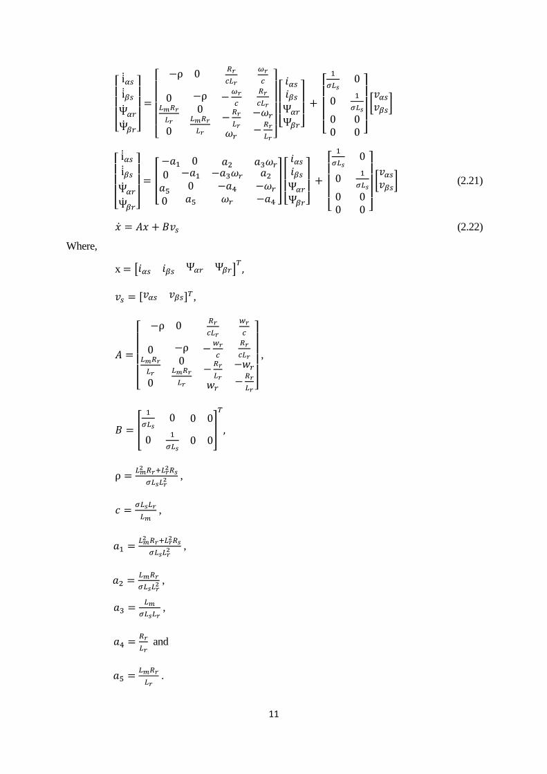
�̇� = 𝐴𝑥 + 𝐵𝑣𝑠 (2.22)

Where,

x = [𝑖𝛼𝑠 𝑖𝛽𝑠 Ψ𝛼𝑟 Ψ𝛽𝑟]𝑇,

𝑣𝑠 = [𝑣𝛼𝑠 𝑣𝛽𝑠]𝑇,

𝐴 =

[ −⍴ 0

𝑅𝑟

𝑐𝐿𝑟

𝑤𝑟

𝑐

0𝐿𝑚𝑅𝑟

𝐿𝑟

0

−⍴0

𝐿𝑚𝑅𝑟

𝐿𝑟

−𝑤𝑟

𝑐

−𝑅𝑟

𝐿𝑟

𝑤𝑟

𝑅𝑟

𝑐𝐿𝑟

−𝑤𝑟

−𝑅𝑟

𝐿𝑟 ]

,

𝐵 = [

1

𝜎𝐿𝑠0 0 0

01

𝜎𝐿𝑠0 0

]

𝑇

,

ρ =𝐿𝑚2 𝑅𝑟+𝐿𝑟

2𝑅𝑠

𝜎𝐿𝑠𝐿𝑟2 ,

𝑐 =𝜎𝐿𝑠𝐿𝑟

𝐿𝑚 ,

𝑎1 =𝐿𝑚2 𝑅𝑟+𝐿𝑟

2𝑅𝑠

𝜎𝐿𝑠𝐿𝑟2 ,

𝑎2 =𝐿𝑚𝑅𝑟

𝜎𝐿𝑠𝐿𝑟2 ,

𝑎3 =𝐿𝑚

𝜎𝐿𝑠𝐿𝑟 ,

𝑎4 =𝑅𝑟

𝐿𝑟 and

𝑎5 =𝐿𝑚𝑅𝑟

𝐿𝑟 .

12

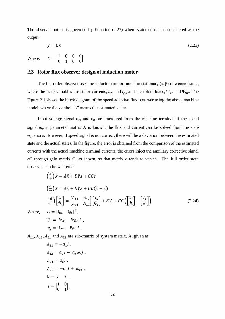
The observer output is governed by Equation (2.23) where stator current is considered as the

output.

𝑦 = 𝐶𝑥 (2.23)

Where, 𝐶 = [1 0 0 00 1 0 0

]

2.3 Rotor flux observer design of induction motor

The full order observer uses the induction motor model in stationary (α-β) reference frame,

where the state variables are stator currents, 𝑖𝛼𝑠 and 𝑖𝛽𝑠 and the rotor fluxes, Ψ𝛼𝑟 and Ψ𝛽𝑟. The

Figure 2.1 shows the block diagram of the speed adaptive flux observer using the above machine

model, where the symbol “˄” means the estimated value.

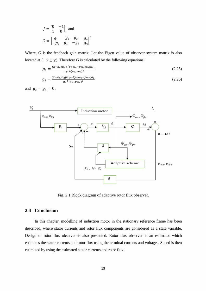
Input voltage signal 𝑣𝛼𝑠 and 𝑣𝛽𝑠 are measured from the machine terminal. If the speed

signal 𝜔𝑟 in parameter matrix A is known, the flux and current can be solved from the state

equations. However, if speed signal is not correct, there will be a deviation between the estimated

state and the actual states. In the figure, the error is obtained from the comparison of the estimated

currents with the actual machine terminal currents, the errors inject the auxiliary corrective signal

eG through gain matrix G, as shown, so that matrix e tends to vanish. The full order state

observer can be written as

(𝑑

𝑑𝑡) �̂� = �̂��̂� + 𝐵𝑉𝑠 + 𝐺𝐶𝑒

(𝑑

𝑑𝑡) �̂� = �̂��̂� + 𝐵𝑉𝑠 + 𝐺𝐶(�̂� − 𝑥)

(𝑑

𝑑𝑡) [

𝑖̂𝑠�̂�𝑟

] = [𝐴11 𝐴12

𝐴21 𝐴22] [

𝑖̂𝑠�̂�𝑟

] + 𝐵𝑉𝑠 + 𝐺𝐶 ([𝑖̂𝑠�̂�𝑟

] − [𝑖𝑠Ψ𝑟

]) (2.24)

Where, 𝑖𝑠 = [𝑖𝛼𝑠 𝑖𝛽𝑠]𝑇,

Ψ𝑟 = [Ψ𝛼𝑟 Ψ𝛽𝑟]𝑇 ,

𝑣𝑠 = [𝑣𝛼𝑠 𝑣𝛽𝑠]𝑇 ,

𝐴11, 𝐴12, 𝐴21 and 𝐴22 are sub-matrix of system matrix, A, given as

𝐴11 = −𝑎1𝐼 ,

𝐴12 = 𝑎2𝐼 − 𝑎3𝜔𝑟𝐽 ,

𝐴21 = 𝑎5𝐼 ,

𝐴22 = −𝑎4𝐼 + 𝜔𝑟𝐽 ,

𝐶 = [𝐼 0] ,

𝐼 = [1 00 1

] ,

13

𝐽 = [0 −11 0

] and

𝐺 = [𝑔1

𝑔2 𝑔3 𝑔4

−𝑔2𝑔1 −𝑔4 𝑔3

]𝑇

Where, G is the feedback gain matrix. Let the Eigen value of observer system matrix is also

located at (−𝑥 ± 𝑦). Therefore G is calculated by the following equations:

𝑔1 =(𝑥−𝑎4)𝑎2+(𝑦+𝜔𝑒−𝑝𝜔𝑟)𝑎3𝑝𝜔𝑟

𝑎22+(𝑎3𝑝𝜔𝑟)2

(2.25)

𝑔2 =(𝑥−𝑎4)𝑎3𝑝𝜔𝑟−(𝑦+𝜔𝑒−𝑝𝜔𝑟)𝑎2

𝑎22+(𝑎3𝑝𝜔𝑟)2

(2.26)

and 𝑔3 = 𝑔4 = 0 .

Fig. 2.1 Block diagram of adaptive rotor flux observer.

2.4 Conclusion

In this chapter, modelling of induction motor in the stationary reference frame has been

described, where stator currents and rotor flux components are considered as a state variable.

Design of rotor flux observer is also presented. Rotor flux observer is an estimator which

estimates the stator currents and rotor flux using the terminal currents and voltages. Speed is then

estimated by using the estimated stator currents and rotor flux.

14

Chapter 3

ADAPTIVE SCHEMES FOR SPEED ESTIMATION AND PARAMETER

IDENTIFICATION FOR FIELD ORIENTED INDUCTION MOTOR

DRIVE

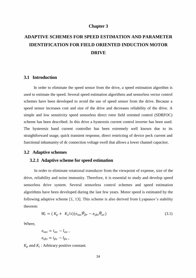
3.1 Introduction

In order to eliminate the speed sensor from the drive, a speed estimation algorithm is

used to estimate the speed. Several speed estimation algorithms and sensorless vector control

schemes have been developed to avoid the use of speed sensor from the drive. Because a

speed sensor increases cost and size of the drive and decreases reliability of the drive. A

simple and low sensitivity speed sensorless direct rotor field oriented control (SDRFOC)

scheme has been described. In this drive a hysteresis current control inverter has been used.

The hysteresis band current controller has been extremely well known due to its

straightforward usage, quick transient response, direct restricting of device peck current and

functional inhumanity of dc connection voltage swell that allows a lower channel capacitor.

3.2 Adaptive schemes

3.2 .1 Adaptive scheme for speed estimation

In order to eliminate rotational transducer from the viewpoint of expense, size of the

drive, reliability and noise immunity. Therefore, it is essential to study and develop speed

sensorless drive system. Several sensorless control schemes and speed estimation

algorithms have been developed during the last few years. Motor speed is estimated by the

following adaptive scheme [1, 13]. This scheme is also derived from Lyapunov’s stability

theorem:

𝑊𝑟 = ( 𝐾𝑝 + 𝐾𝑖/𝑠)(𝑒𝑖𝛼𝑠�̂�𝛽𝑟 − 𝑒𝑖𝛽𝑠�̂�𝛼𝑟) (3.1)

Where,

𝑒𝑖𝛼𝑠 = 𝑖𝛼𝑠 − 𝑖̂𝛼𝑠 ,

𝑒𝑖𝛽𝑠 = 𝑖𝛽𝑠 − 𝑖�̂�𝑠 ,

𝐾𝑝 and 𝐾𝑖 : Arbitrary positive constant.

15

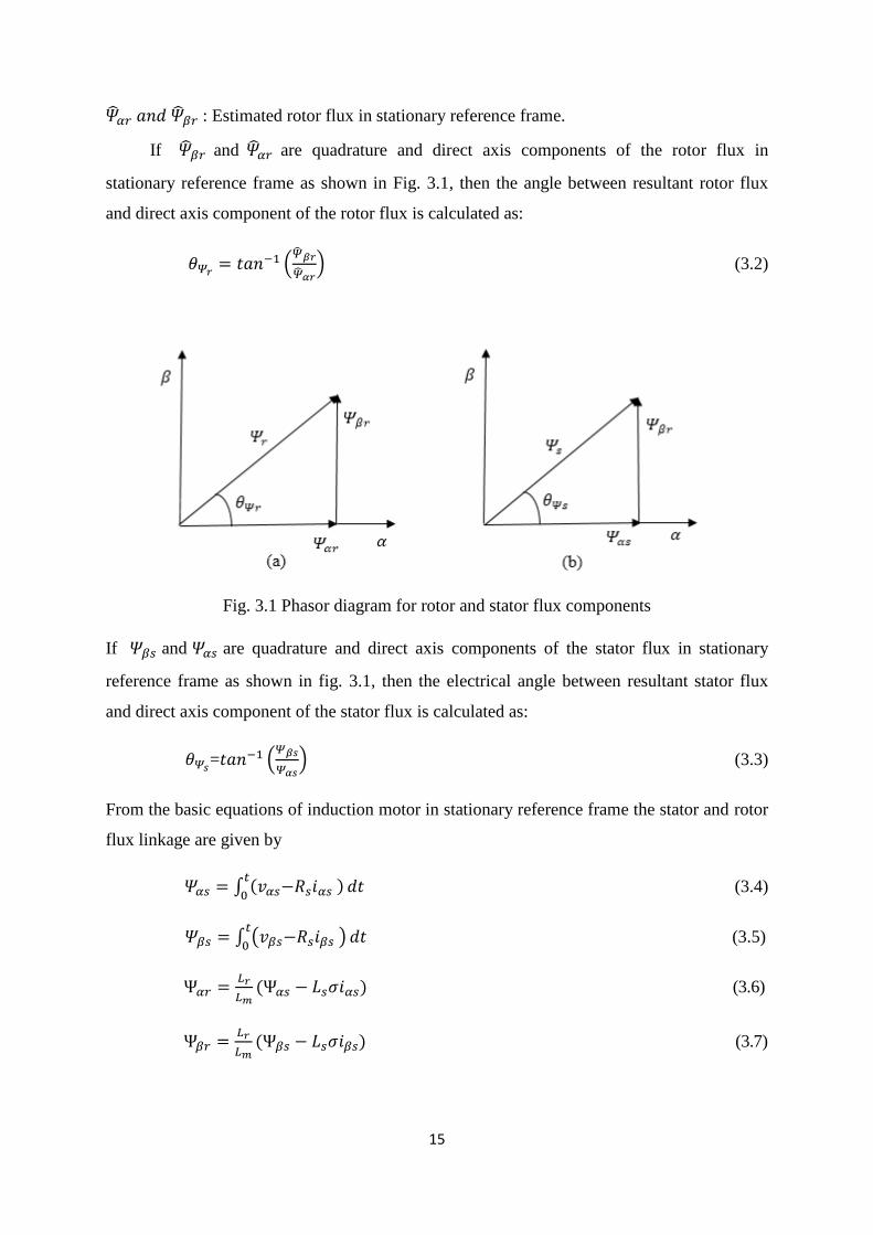
�̂�𝛼𝑟 𝑎𝑛𝑑 �̂�𝛽𝑟 : Estimated rotor flux in stationary reference frame.

If �̂�𝛽𝑟 and �̂�𝛼𝑟 are quadrature and direct axis components of the rotor flux in

stationary reference frame as shown in Fig. 3.1, then the angle between resultant rotor flux

and direct axis component of the rotor flux is calculated as:

𝜃𝛹𝑟= 𝑡𝑎𝑛−1 (

�̂�𝛽𝑟

�̂�𝛼𝑟) (3.2)

Fig. 3.1 Phasor diagram for rotor and stator flux components

If 𝛹𝛽𝑠 and 𝛹𝛼𝑠 are quadrature and direct axis components of the stator flux in stationary

reference frame as shown in fig. 3.1, then the electrical angle between resultant stator flux

and direct axis component of the stator flux is calculated as:

𝜃𝛹𝑠=𝑡𝑎𝑛−1 (

𝛹𝛽𝑠

𝛹𝛼𝑠) (3.3)

From the basic equations of induction motor in stationary reference frame the stator and rotor

flux linkage are given by

𝛹𝛼𝑠 = ∫ (𝑣𝛼𝑠−𝑅𝑠𝑖𝛼𝑠 )𝑡

0𝑑𝑡 (3.4)

𝛹𝛽𝑠 = ∫ (𝑣𝛽𝑠−𝑅𝑠𝑖𝛽𝑠 )𝑡

0𝑑𝑡 (3.5)

Ψ𝛼𝑟 =𝐿𝑟

𝐿𝑚(Ψ𝛼𝑠 − 𝐿𝑠𝜎𝑖𝛼𝑠) (3.6)

Ψ𝛽𝑟 =𝐿𝑟

𝐿𝑚(Ψ𝛽𝑠 − 𝐿𝑠𝜎𝑖𝛽𝑠) (3.7)

16

The equations (3.4) and (3.4) show that the stator flux relies on the stator resistance and measured

stator voltages and currents. The equations (3.6) and (3.7) show that the rotor flux relies on stator

flux and the stator leakage inductance (𝐿𝑠).

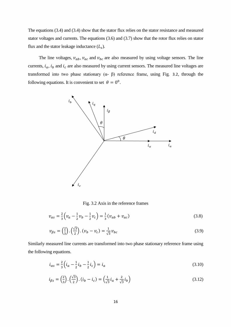
The line voltages, 𝑣𝑎𝑏, 𝑣𝑎𝑐 and 𝑣𝑏𝑐 are also measured by using voltage sensors. The line

currents, 𝑖𝑎, 𝑖𝑏 and 𝑖𝑐 are also measured by using current sensors. The measured line voltages are

transformed into two phase stationary (α- β) reference frame, using Fig. 3.2, through the

following equations. It is convenient to set 𝜃 = 00.

Fig. 3.2 Axis in the reference frames

𝑣𝛼𝑠 =2

3(𝑣𝑎 −

1

2𝑣𝑏 −

1

2𝑣𝑐) =

1

3(𝑣𝑎𝑏 + 𝑣𝑎𝑐) (3.8)

𝑣𝛽𝑠 = (2

3) . (

√3

2) . (𝑣𝑏 − 𝑣𝑐) =

1

√3𝑣𝑏𝑐 (3.9)

Similarly measured line currents are transformed into two phase stationary reference frame using

the following equations.

𝑖𝛼𝑠 =2

3(𝑖𝑎 −

1

2𝑖𝑏 −

1

2𝑖𝑐) = 𝑖𝑎 (3.10)

𝑖𝛽𝑠 = (2

3) . (

√3

2) . (𝑖𝑏 − 𝑖𝑐) = (

1

√3𝑖𝑎 +

2

√3𝑖𝑏) (3.12)

17

3.2 .2 Adaptive scheme for stator and rotor resistance

There are also several methods to estimate the stator resistance and rotor time constant

simultaneously [1]. The stator resistance and rotor time constant which vary with

temperature. Hence it causes loss in the motor and decreases the motor efficiency and causes

instability problem. To reduce these effect simultaneous estimation of stator resistance and

rotor time constant is required. Stator resistance can be estimated by the given equation:

(𝑑

𝑑𝑡) �̂�𝑠 = −𝜆1(𝑒𝑖𝛼𝑠𝑖̂𝛼𝑠 + 𝑒𝑖𝛽𝑠𝑖�̂�𝑠) (3.13)

(𝑑

𝑑𝑡) (1 �̂�𝑟)⁄ = (

𝜆2

𝐿𝑟 ) {𝑒𝑖𝛼𝑠(�̂�𝛼𝑟 − 𝑀𝑖̂𝛼𝑠) + 𝑒𝑖𝛽𝑠(�̂�𝛽𝑟 − 𝑀𝑖�̂�𝑠)} (3.14)

Where,

𝑒𝑖𝛼𝑠 = 𝑖𝛼𝑠 − 𝑖̂𝛼𝑠, 𝑒𝑖𝛽𝑠 = 𝑖𝛽𝑠 − 𝑖�̂�𝑠, λ1 and λ2: arbitrary positive gain.

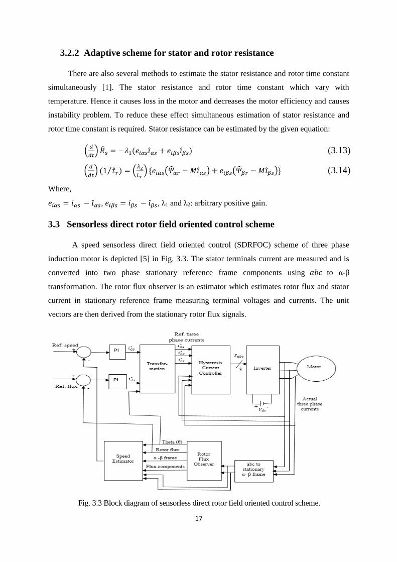
3.3 Sensorless direct rotor field oriented control scheme

A speed sensorless direct field oriented control (SDRFOC) scheme of three phase

induction motor is depicted [5] in Fig. 3.3. The stator terminals current are measured and is

converted into two phase stationary reference frame components using 𝑎𝑏𝑐 to α-β

transformation. The rotor flux observer is an estimator which estimates rotor flux and stator

current in stationary reference frame measuring terminal voltages and currents. The unit

vectors are then derived from the stationary rotor flux signals.

Fig. 3.3 Block diagram of sensorless direct rotor field oriented control scheme.

18

The speed control loop produces the torque component of stator current. The reference

speed is contrasted with the estimated speed and the velocity error is fed to a PI controller in

the speed control loop. The controller generates 𝑖𝑞𝑠∗ taking into account this speed error.

Where, 𝑖𝑞𝑠∗ is known as torque component of stator reference current. So also a flux control

loop is likewise included to improve the flux control accuracy. The flux component and

torque component of stator current are converted to three phase quantities utilizing the unit

vectors. These three phase currents are fed as reference values to the hysteresis band current

controller. The switching signals for the inverter switches are generated from the controller,

from the comparison of the current error signal with a fixed width hysteresis band.

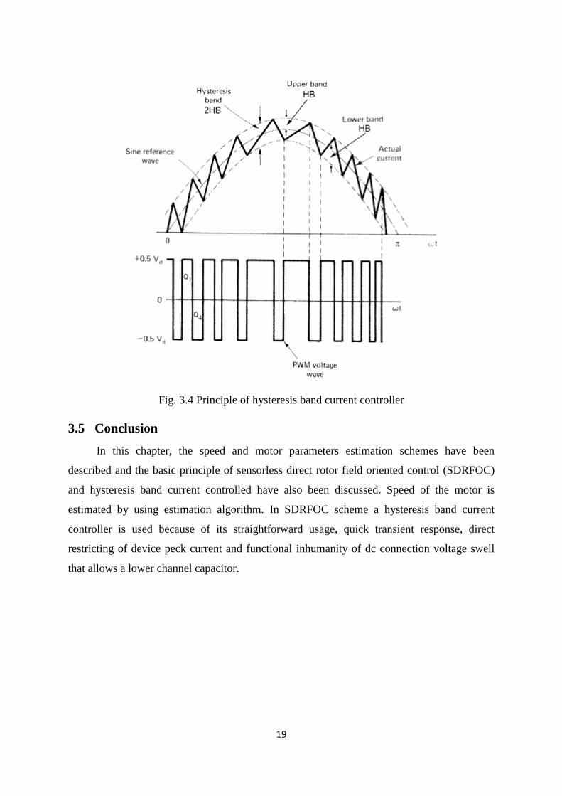
3.4 Hysteresis band current control PWM

In industrial application, the current controlled PWM inverters are extensively used in

ac motor drives. The main purpose of the control systems in current controlled inverters is to

force the current vector in the three phase load according to a reference trajectory. This is

presented in Fig. 3.4 for a half bridge inverter [13]. Where the reference current is contrasted

with the actual phase current. When the actual current tries to go beyond the upper tolerance

band, the upper switch in the half bridge is turned off and lower switch is turned on.

Accordingly the output voltage changes from +0.5𝑉𝑑 to -0.5𝑉𝑑 and the current starts to decay.

Similarly when the actual phase current tries to go beyond the lower tolerance band, the

lower switch is turned off and the upper switch is turned on. As a result, output voltage

transition from -0.5𝑉𝑑 to +0.5𝑉𝑑 and current starts to increase.

The conditions for switching the devices are:

Upper switch on: (𝑖∗ − 𝑖) > 𝐻𝐵

Lower switch on: (𝑖∗ − 𝑖) < −𝐻𝐵

Where,

𝑖∗ = Reference current;

𝑖 = Actual phase current;

𝐻𝐵 = Hysteresis band.

For three phase inverter, a similar control scheme is used in all phases.

19

Fig. 3.4 Principle of hysteresis band current controller

3.5 Conclusion

In this chapter, the speed and motor parameters estimation schemes have been

described and the basic principle of sensorless direct rotor field oriented control (SDRFOC)

and hysteresis band current controlled have also been discussed. Speed of the motor is

estimated by using estimation algorithm. In SDRFOC scheme a hysteresis band current

controller is used because of its straightforward usage, quick transient response, direct

restricting of device peck current and functional inhumanity of dc connection voltage swell

that allows a lower channel capacitor.

20

Chapter- 4

AXES TRANSFORMATION

4.1 Introduction

Mathematical transformations are devices which make complex framework easy to

study and easy to focus. In electrical machines analysis, a three phase variables to two phase

variables transformation is applied to produce less complex expressions that provide more

understanding into the cooperation of the distinctive parameters. In this chapter, the various

transformations studied in the past have been presented.

4.2 General change of variables in transformations

Consider a symmetrical three phase induction machine with stationary three axes at

2ᴨ/3 angle apart as shown in Fig. 4.1. The real three phase supply system cane be represented

by these three axes. Whereas, the two axes are representing two fictitious phases

perpendicular to one other. The change of three phase variables to two phase variables [13 ]

can be possible in such a way that the two phase variables are either in a stationary reference

frame or in synchronously rotating reference frame. Transformation into a syncronously

pivoted rotating reference frame is more common and it can be possible with the

transformation of the three phase variables into two phase variables and after that transform

these to synchronously moving reference frame. Speed of the stationary reference frame is

zero, whereas speed of synchronously rotating reference frame is same as supply frequency.

The stationary reference frame variables are appeared as a dc value in synchronously rotating

reference frame instead of time varying quantities.

4.2 .1 Transformation into a stationary reference frame

It is considered that the three phase axes and the two phase axes are in a stationary

reference frame. Our aim is to transform the three phase (abc) variables to two phase (αβ0)

variables. The relationship between three phase variables and two phase variables in

stationary reference frame is given below and the transformation from three phase statiory

reference frame to two phase stationary reference frame [13] can be understood from Fig. 4.1.

21

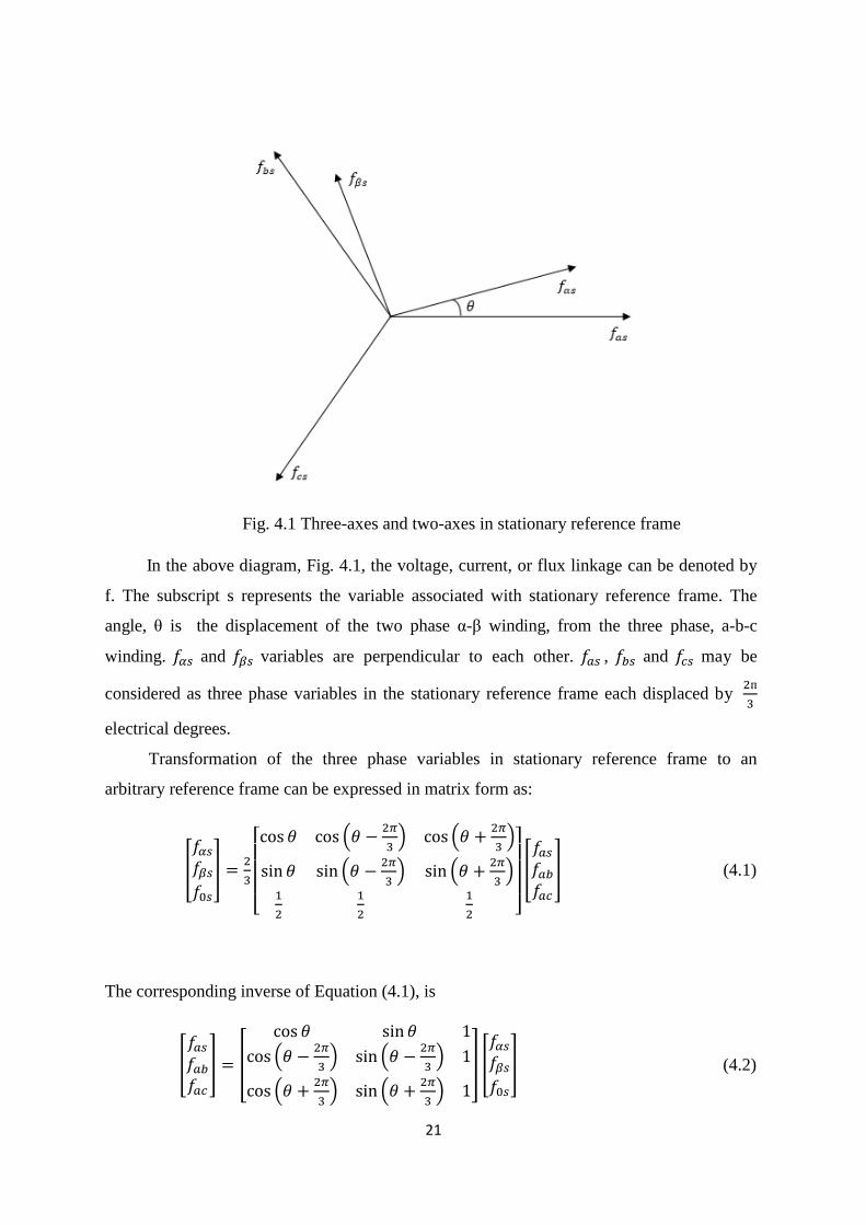
Fig. 4.1 Three-axes and two-axes in stationary reference frame

In the above diagram, Fig. 4.1, the voltage, current, or flux linkage can be denoted by

f. The subscript s represents the variable associated with stationary reference frame. The

angle, θ is the displacement of the two phase α-β winding, from the three phase, a-b-c

winding. 𝑓𝛼𝑠 and 𝑓𝛽𝑠 variables are perpendicular to each other. 𝑓𝑎𝑠 , 𝑓𝑏𝑠 and 𝑓𝑐𝑠 may be

considered as three phase variables in the stationary reference frame each displaced by 2ᴨ

3

electrical degrees.

Transformation of the three phase variables in stationary reference frame to an

arbitrary reference frame can be expressed in matrix form as:

[

𝑓𝛼𝑠

𝑓𝛽𝑠

𝑓0𝑠

] =2

3

[ cos 𝜃 cos (𝜃 −

2𝜋

3) cos (𝜃 +

2𝜋

3)

sin 𝜃 sin (𝜃 −2𝜋

3) sin (𝜃 +

2𝜋

3)

1

2

1

2

1

2 ]

[

𝑓𝑎𝑠

𝑓𝑎𝑏

𝑓𝑎𝑐

] (4.1)

The corresponding inverse of Equation (4.1), is

[

𝑓𝑎𝑠

𝑓𝑎𝑏

𝑓𝑎𝑐

] = [

cos 𝜃 sin 𝜃 1

cos (𝜃 −2𝜋

3) sin (𝜃 −

2𝜋

3) 1

cos (𝜃 +2𝜋

3) sin (𝜃 +

2𝜋

3) 1

] [

𝑓𝛼𝑠

𝑓𝛽𝑠

𝑓0𝑠

] (4.2)

22

It is convenient to set 𝜃 = 0, so that the α-axis is aligned with the a-axis. Therefore the

Equation (4.1) will be written as

[

𝑓𝛼𝑠

𝑓𝛽𝑠

𝑓0𝑠

] =2

3

[ 1 −

1

2−

1

2

0 −√3

2

√3

21

2

1

2

1

2 ]

[

𝑓𝑎𝑠

𝑓𝑎𝑏

𝑓𝑎𝑐

] (4.3)

and Equation (4.2) will be simplified to

[

𝑓𝑎𝑠

𝑓𝑎𝑏

𝑓𝑎𝑐

] =

[

1 0 1

−1

2−

√3

21

−1

2

√3

21]

[

𝑓𝛼𝑠

𝑓𝛽𝑠

𝑓0𝑠

] (4.4)

Equations (4.3) and (4.4) shows that the magnitude of the phase quantities, voltages and

currents, in the three phase stationary reference frame (a-b-c) variables and two phase

stationary reference frame (d-q) variables remain the same. In this transformation, it is

considred that the number of turns in each phase of the three phase winding and the two

phase winding are same.

4.2 .2 Transformation into rotating reference frame

The rotating frame o f reference c a n have any speed of rotation subjected to the

requirment of the system. If the speed of the roatating reference frame matches wih the

frequencey of excitation current, then all the transformed variables of instataneous values

will appear as constant quantity. Thus it can be stated that if an observer moves along with

the same speed then the space vector looks as three dimension with steady state. The speed of

rotation for the reference frame must be same as the observer. For two dimensional variables

any two independent basic space vectors can be taken as reference. These are denoted by

another pair of orthogonal d-q axes. The zero-sequence elements remains unchanged. The

stationary reference frame a-b-c variables converted to the rotating reference frame d-q

variables occurs in two steps, i.e., first transforming to stationary α-β variables and then to

rotating d-q variables. The axes transformation from abc to dq0 is shown in Fig. 4.2.

23

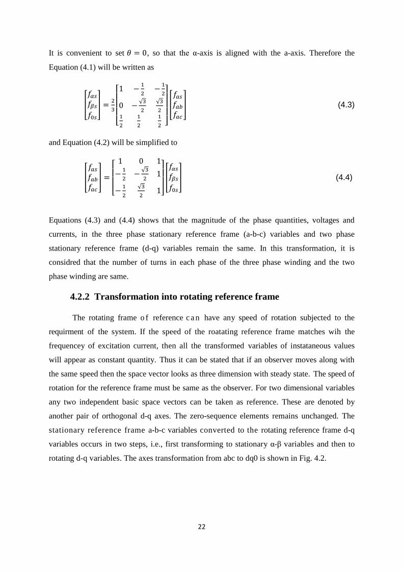
Fig. 4.2 Shows steps of the a-b-c to rotating d-q axes transformation: (a) a-b-c to stationary

α- β axes and (b) stationary α-β to rotating d-q axes.

The equation for the stationary reference frame α-β variables to rotating reference frame d-q

variables transformation [13] is given in Equation (4.5). Utilizing geometry, the relation

between the stationary α-β axes and rotating d-q axes can be expressed as:

[𝑓𝑑

𝑓𝑞] = [

cos 𝜃 sin 𝜃−sin 𝜃 cos 𝜃

] [𝑓𝛼𝑓𝛽

] (4 .5 )

The angle, θ, is t h e displacement between the two phase stationary reference frame α-β

and two phase rotating reference frame d-q. The angular speed, ω (t), of the rotating reference

frame d-q can be represented with theta (θ) function. The initial values are written as

𝜃(𝑡) = ∫ 𝜔(𝑡) 𝑑𝑡𝑡

0+ 𝜃(0) (4 .6)

Three phase voltages and currents in stationary reference frame can be obtained by

applying two phase stationary reference frame, α-β to three phase stationary reference frame,

a-b-c transformation equations as above explained

[

𝑓𝑎𝑓𝑏

𝑓𝑐

] =

[

1 0

−1

2−

√3

2

−1

2

√3

2 ]

[𝑓𝛼𝑓𝛽

] (4.7)

24

The three phase voltage or current quantities in stationary reference frame are represented

by 𝑓𝑎, 𝑓𝑏 and 𝑓𝑐 and the two-phase voltage or current quantities in stationary reference frame

are represented by 𝑓𝛼 and 𝑓𝛽.

4.3 Conclusion

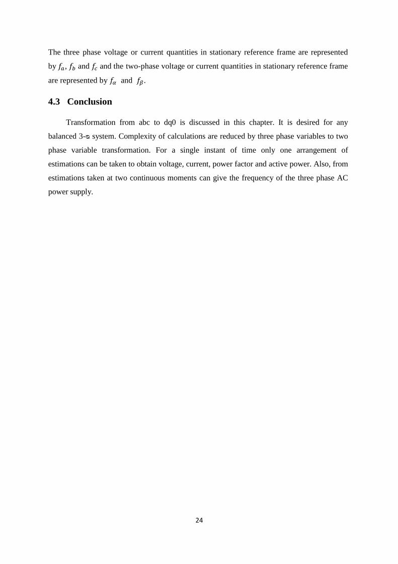
Transformation from abc to dq0 is discussed in this chapter. It is desired for any

balanced 3-ᴓ system. Complexity of calculations are reduced by three phase variables to two

phase variable transformation. For a single instant of time only one arrangement of

estimations can be taken to obtain voltage, current, power factor and active power. Also, from

estimations taken at two continuous moments can give the frequency of the three phase AC

power supply.

25

Chapter-5

SIMULATION RESULTS AND DISCUSSION

5.1 Introduction

A Simulink model of speed sensorless vector control for three phase induction motor

has been developed in MATLAB, Simulink. Different speed, current and flux graph have

been plotted in different speed and load torque.

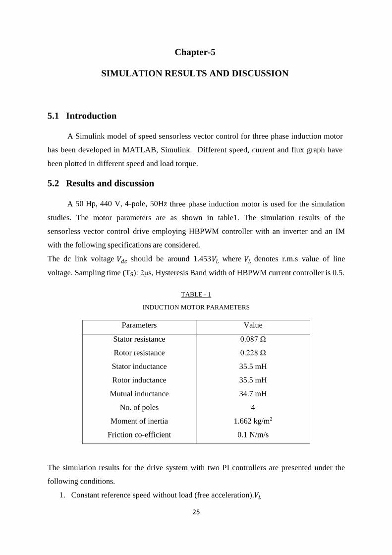
5.2 Results and discussion

A 50 Hp, 440 V, 4-pole, 50Hz three phase induction motor is used for the simulation

studies. The motor parameters are as shown in table1. The simulation results of the

sensorless vector control drive employing HBPWM controller with an inverter and an IM

with the following specifications are considered.

The dc link voltage 𝑉𝑑𝑐 should be around 1.453𝑉𝐿 where 𝑉𝐿 denotes r.m.s value of line

voltage. Sampling time (Ts): 2μs, Hysteresis Band width of HBPWM current controller is 0.5.

TABLE - 1

INDUCTION MOTOR PARAMETERS

Parameters Value

Stator resistance

Rotor resistance

Stator inductance

Rotor inductance

Mutual inductance

No. of poles

Moment of inertia

Friction co-efficient

0.087 Ω

0.228 Ω

35.5 mH

35.5 mH

34.7 mH

4

1.662 kg/m2

0.1 N/m/s

The simulation results for the drive system with two PI controllers are presented under the

following conditions.

1. Constant reference speed without load (free acceleration).𝑉𝐿

26

2. Constant reference speed with load.

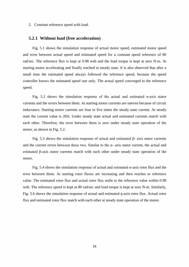
5.2 .1 Without load (free acceleration)

Fig. 5.1 shows the simulation response of actual motor speed, estimated motor speed

and error between actual speed and estimated speed for a constant speed reference of 80

rad/sec. The reference flux is kept at 0.98 web and the load torque is kept at zero N-m. At

starting motor accelerating and finally reached to steady state. It is also observed that after a

small time the estimated speed always followed the reference speed, because the speed

controller knows the estimated speed one only. The actual speed converged to the reference

speed.

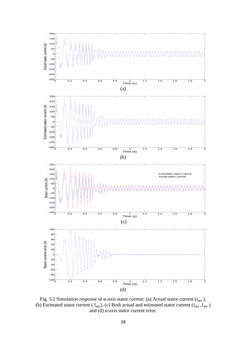
Fig. 5.2 shows the simulation response of the actual and estimated α-axis stator

currents and the errors between them. At starting motor currents are uneven because of circuit

inductance. Starting motor currents are four to five times the steady state current. At steady

state the current value is 28A. Under steady state actual and estimated currents match with

each other. Therefore, the error between them is zero under steady state operation of the

motor, as shown in Fig. 5.2.

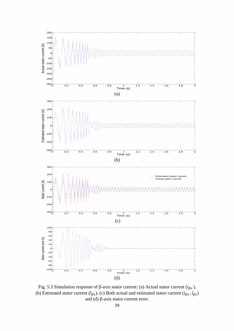
Fig. 5.3 shows the simulation response of actual and estimated β- axis stator currents

and the current errors between these two. Similar to the α- axis stator current, the actual and

estimated β-axis stator currents match with each other under steady state operation of the

motor.

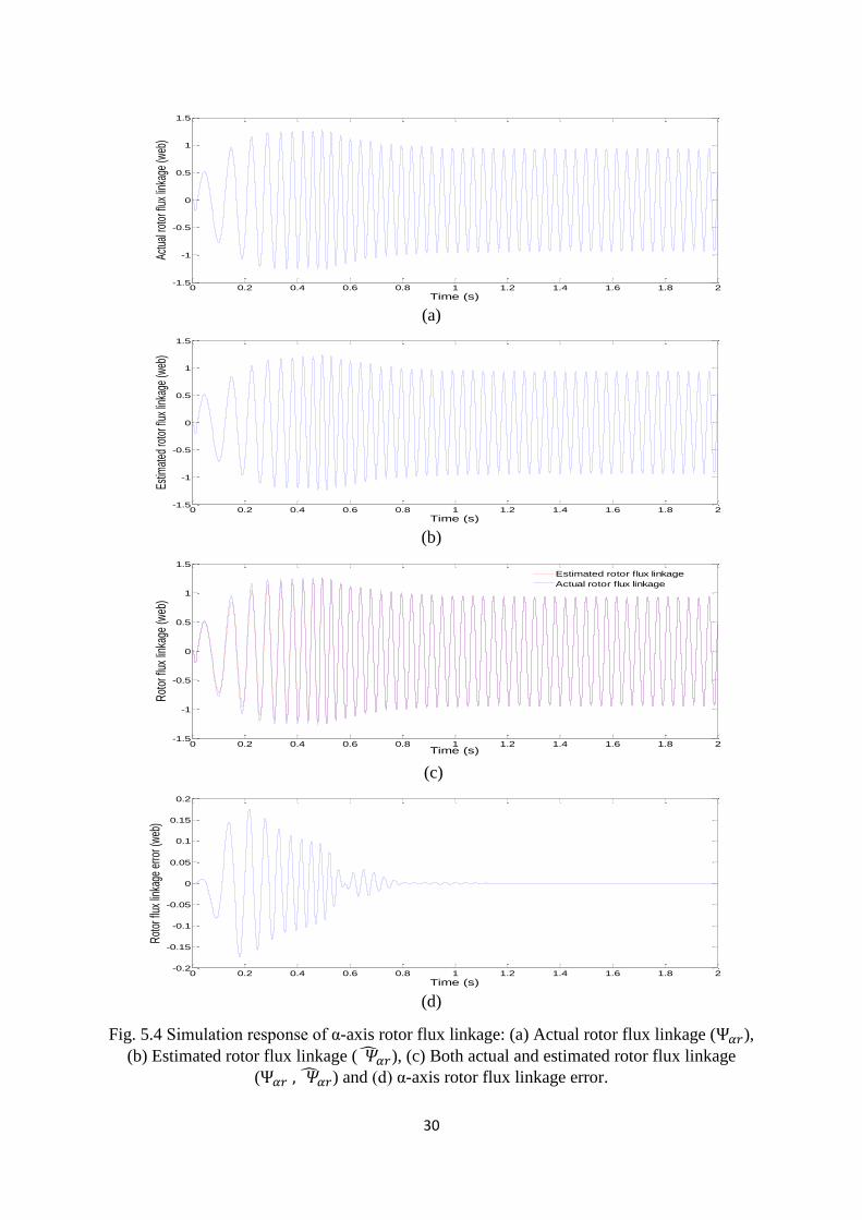
Fig. 5.4 shows the simulation response of actual and estimated α-axis rotor flux and the

error between them. At starting rotor fluxes are increasing and then reaches to reference

value. The estimated rotor flux and actual rotor flux settle to the reference value within 0.98

web. The reference speed is kept at 80 rad/sec and load torque is kept at zero N-m. Similarly,

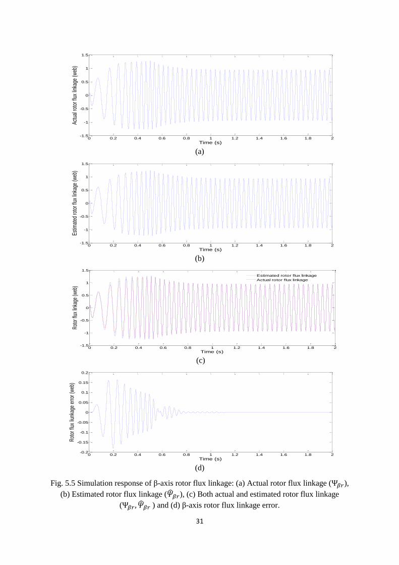
Fig. 5.6 shows the simulation response of actual and estimated q-axis rotor flux. Actual rotor

flux and estimated rotor flux match with each other at steady state operation of the motor.

27

(a)

(b)

(c)

(d)

Fig. 5.1 Simulation response of rotor speed: (a) Actual rotor speed (𝜔𝑟), (b) Estimated rotor

speed (�̂�𝑟), (c) Actual and estimated rotor speed (𝜔𝑟, �̂�𝑟) and (d) Speed error.

0 0.5 1 1.5 2 2.5-10

0

10

20

30

40

50

60

70

80

90

Time (s)

Act

ual r

otor

spe

ed (r

ad/s

)

0 0.5 1 1.5 2 2.5-10

0

10

20

30

40

50

60

70

80

90

Time (s)

Est

imat

ed ro

tor s

pedd

(rad

/s)

0 0.5 1 1.5 2 2.5-10

0

10

20

30

40

50

60

70

80

90

Time (s)

Rot

or s

peed

(rad

/s)

Estimated rotor speed

Actual rotor speed

0 0.5 1 1.5 2 2.5-4

-2

0

2

4

6

8

10

12

14

Time (s)

Spee

d er

ror (

rad/

s)

28

(a)

(b)

(c)

(d)

Fig. 5.2 Simulation response of α-axis stator current: (a) Actual stator current (𝑖𝛼𝑠 ),

(b) Estimated stator current ( 𝑖̂𝛼𝑠), (c) Both actual and estimated stator current (𝑖𝛼𝑠 , 𝑖̂𝛼𝑠 )

and (d) α-axis stator current error.

0 0.2 0.4 0.6 0.8 1 1.2 1.4 1.6 1.8 2-250

-200

-150

-100

-50

0

50

100

150

200

Time (s)

Actu

al s

tato

r cur

rent

(A)

0 0.2 0.4 0.6 0.8 1 1.2 1.4 1.6 1.8 2-250

-200

-150

-100

-50

0

50

100

150

200

250

Time (s)

Est

imat

ed s

tato

r cur

rent

(A)

0 0.2 0.4 0.6 0.8 1 1.2 1.4 1.6 1.8 2-250

-200

-150

-100

-50

0

50

100

150

200

250

Time (s)

Stat

or c

urre

nt (A

)

Estimated stator current

Actual stator current

0 0.2 0.4 0.6 0.8 1 1.2 1.4 1.6 1.8 2-100

-80

-60

-40

-20

0

20

40

60

80

100

Time (s)

Sta

tor c

urre

nt e

rror

(A)

29

(a)

(b)

(c)

(d)

Fig. 5.3 Simulation response of β-axis stator current: (a) Actual stator current (𝑖𝛽𝑠 ),

(b) Estimated stator current (𝑖�̂�𝑠), (c) Both actual and estimated stator current (𝑖𝛽𝑠 , 𝑖�̂�𝑠)

and (d) β-axis stator current error.

0 0.2 0.4 0.6 0.8 1 1.2 1.4 1.6 1.8 2-300

-250

-200

-150

-100

-50

0

50

100

150

200

Time (s)

Act

ual s

tato

r cu

rren

t (A

)

0 0.2 0.4 0.6 0.8 1 1.2 1.4 1.6 1.8 2-300

-200

-100

0

100

200

300

Time (s)

Est

imat

ed s

tato

r cur

rent

(A)

0 0.2 0.4 0.6 0.8 1 1.2 1.4 1.6 1.8 2-300

-200

-100

0

100

200

300

Time (s)

Stat

or c

urre

nt (A

)

Estimated stator current

Actual stator current

0 0.2 0.4 0.6 0.8 1 1.2 1.4 1.6 1.8 2-100

-80

-60

-40

-20

0

20

40

60

80

100

Time (s)

Stat

or c

urre

nt e

rror (

A)

30

(a)

(b)

(c)

(d)

Fig. 5.4 Simulation response of α-axis rotor flux linkage: (a) Actual rotor flux linkage (Ψ𝛼𝑟),

(b) Estimated rotor flux linkage ( �̂�𝛼𝑟), (c) Both actual and estimated rotor flux linkage

(Ψ𝛼𝑟 , �̂�𝛼𝑟) and (d) α-axis rotor flux linkage error.

0 0.2 0.4 0.6 0.8 1 1.2 1.4 1.6 1.8 2-1.5

-1

-0.5

0

0.5

1

1.5

Time (s)

Actu

al ro

tor f

lux

linka

ge (w

eb)

0 0.2 0.4 0.6 0.8 1 1.2 1.4 1.6 1.8 2-1.5

-1

-0.5

0

0.5

1

1.5

Time (s)

Estim

ated

roto

r flu

x lin

kage

(web

)

0 0.2 0.4 0.6 0.8 1 1.2 1.4 1.6 1.8 2-1.5

-1

-0.5

0

0.5

1

1.5

Time (s)

Rot

or fl

ux li

nkag

e (w

eb)

Estimated rotor flux linkage

Actual rotor flux linkage

0 0.2 0.4 0.6 0.8 1 1.2 1.4 1.6 1.8 2-0.2

-0.15

-0.1

-0.05

0

0.05

0.1

0.15

0.2

Time (s)

Rot

or fl

ux li

nkag

e er

ror (

web

)

31

(a)

(b)

(c)

(d)

Fig. 5.5 Simulation response of β-axis rotor flux linkage: (a) Actual rotor flux linkage (Ψ𝛽𝑟),

(b) Estimated rotor flux linkage (�̂�𝛽𝑟), (c) Both actual and estimated rotor flux linkage

(Ψ𝛽𝑟 , �̂�𝛽𝑟 ) and (d) β-axis rotor flux linkage error.

0 0.2 0.4 0.6 0.8 1 1.2 1.4 1.6 1.8 2-1.5

-1

-0.5

0

0.5

1

1.5

Time (s)

Act

ual r

otor

flux

link

age

(web

)

0 0.2 0.4 0.6 0.8 1 1.2 1.4 1.6 1.8 2-1.5

-1

-0.5

0

0.5

1

1.5

Time (s)

Estim

ated

roto

r flu

x lin

kage

(web

)

0 0.2 0.4 0.6 0.8 1 1.2 1.4 1.6 1.8 2-1.5

-1

-0.5

0

0.5

1

1.5

Time (s)

Rot

or fl

ux li

nkag

e (w

eb)

Estimated rotor flux linkage

Actual rotor flux linkage

0 0.2 0.4 0.6 0.8 1 1.2 1.4 1.6 1.8 2-0.2

-0.15

-0.1

-0.05

0

0.05

0.1

0.15

0.2

Time (s)

Rot

or fl

ux li

unka

ge e

rror (

web

)

32

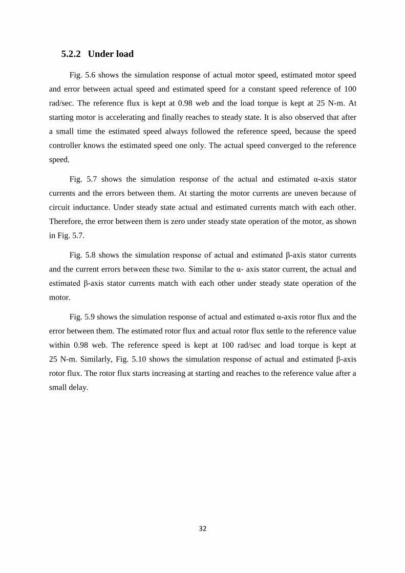
5.2 .2 Under load

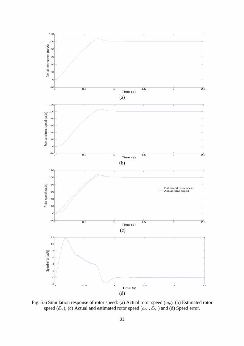
Fig. 5.6 shows the simulation response of actual motor speed, estimated motor speed

and error between actual speed and estimated speed for a constant speed reference of 100

rad/sec. The reference flux is kept at 0.98 web and the load torque is kept at 25 N-m. At

starting motor is accelerating and finally reaches to steady state. It is also observed that after

a small time the estimated speed always followed the reference speed, because the speed

controller knows the estimated speed one only. The actual speed converged to the reference

speed.

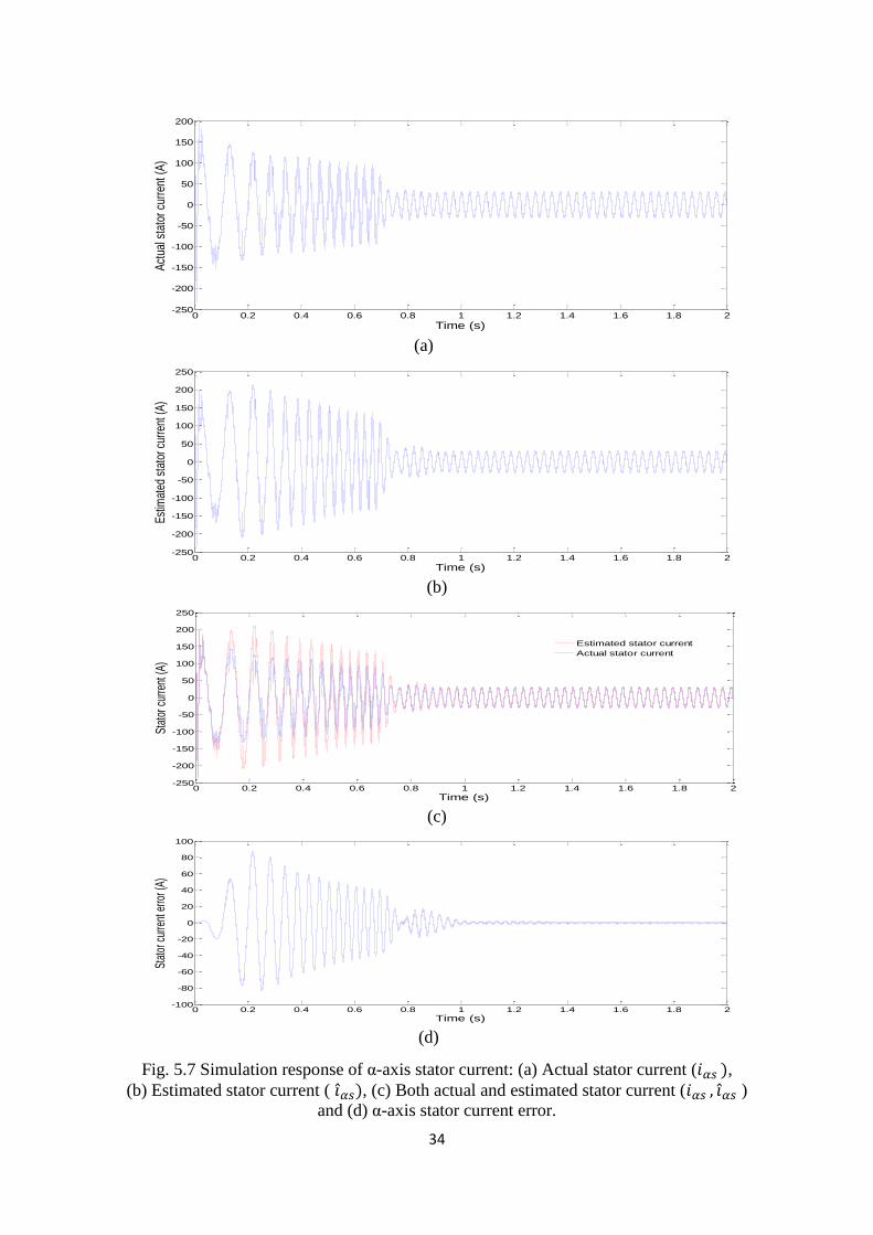
Fig. 5.7 shows the simulation response of the actual and estimated α-axis stator

currents and the errors between them. At starting the motor currents are uneven because of

circuit inductance. Under steady state actual and estimated currents match with each other.

Therefore, the error between them is zero under steady state operation of the motor, as shown

in Fig. 5.7.

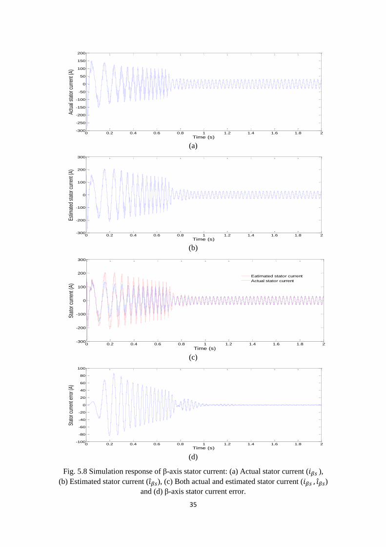
Fig. 5.8 shows the simulation response of actual and estimated β-axis stator currents

and the current errors between these two. Similar to the α- axis stator current, the actual and

estimated β-axis stator currents match with each other under steady state operation of the

motor.

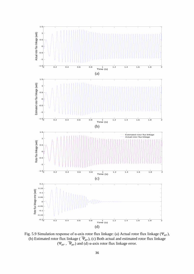
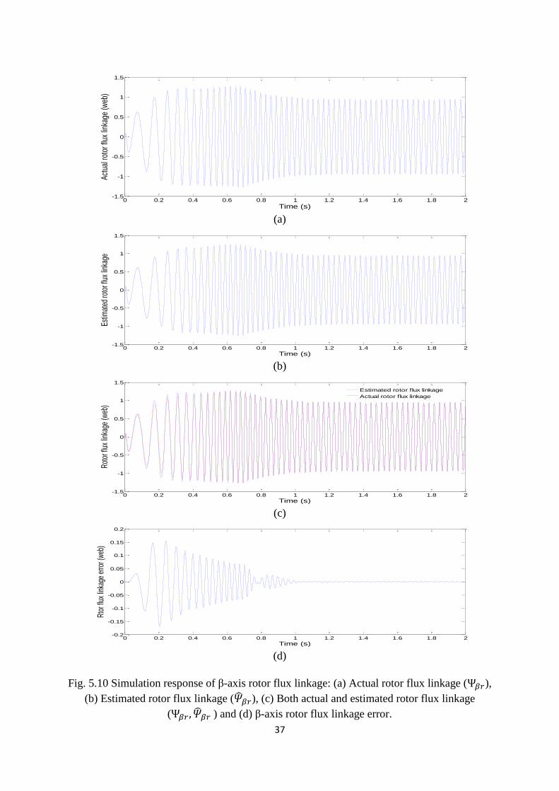
Fig. 5.9 shows the simulation response of actual and estimated α-axis rotor flux and the

error between them. The estimated rotor flux and actual rotor flux settle to the reference value

within 0.98 web. The reference speed is kept at 100 rad/sec and load torque is kept at

25 N-m. Similarly, Fig. 5.10 shows the simulation response of actual and estimated β-axis

rotor flux. The rotor flux starts increasing at starting and reaches to the reference value after a

small delay.

33

(a)

(b)

(c)

(d)

Fig. 5.6 Simulation response of rotor speed: (a) Actual rotor speed (𝜔𝑟), (b) Estimated rotor

speed (�̂�𝑟), (c) Actual and estimated rotor speed (𝜔𝑟 , �̂�𝑟 ) and (d) Speed error.

0 0.5 1 1.5 2 2.5-20

0

20

40

60

80

100

120

Time (s)

Act

ual r

otor

spe

ed (

rad/

s)

0 0.5 1 1.5 2 2.5-20

0

20

40

60

80

100

120

Time (s)

Estim

ated

roto

r spe

ed (r

ad/s

)

0 0.5 1 1.5 2 2.5-20

0

20

40

60

80

100

120

Time (s)

Rot

or s

peed

(rad

/s)

Estimated rotor speed

Actual rotor speed

0 0.5 1 1.5 2 2.5-2

0

2

4

6

8

10

12

Time (s)

Spee

d er

ror (

rad/

s)

34

(a)

(b)

(c)

(d)

Fig. 5.7 Simulation response of α-axis stator current: (a) Actual stator current (𝑖𝛼𝑠 ),

(b) Estimated stator current ( 𝑖̂𝛼𝑠), (c) Both actual and estimated stator current (𝑖𝛼𝑠 , 𝑖̂𝛼𝑠 )

and (d) α-axis stator current error.

0 0.2 0.4 0.6 0.8 1 1.2 1.4 1.6 1.8 2-250

-200

-150

-100

-50

0

50

100

150

200

Time (s)

Act

ual s

tato

r cu

rren

t (A

)

0 0.2 0.4 0.6 0.8 1 1.2 1.4 1.6 1.8 2-250

-200

-150

-100

-50

0

50

100

150

200

250

Time (s)

Est

imat

ed s

tato

r cur

rent

(A)

0 0.2 0.4 0.6 0.8 1 1.2 1.4 1.6 1.8 2-250

-200

-150

-100

-50

0

50

100

150

200

250

Time (s)

Stat

or c

urre

nt (A

)

Estimated stator current

Actual stator current

0 0.2 0.4 0.6 0.8 1 1.2 1.4 1.6 1.8 2-100

-80

-60

-40

-20

0

20

40

60

80

100

Time (s)

Stat

or c

urre

nt e

rror (

A)

35

(a)

(b)

(c)

(d)

Fig. 5.8 Simulation response of β-axis stator current: (a) Actual stator current (𝑖𝛽𝑠 ),

(b) Estimated stator current (𝑖�̂�𝑠), (c) Both actual and estimated stator current (𝑖𝛽𝑠 , 𝑖�̂�𝑠)

and (d) β-axis stator current error.

0 0.2 0.4 0.6 0.8 1 1.2 1.4 1.6 1.8 2-300

-250

-200

-150

-100

-50

0

50

100

150

200

Time (s)

Actu

al s

tato

r cur

rent

(A)

0 0.2 0.4 0.6 0.8 1 1.2 1.4 1.6 1.8 2-300

-200

-100

0

100

200

300

Time (s)

Estim

ated

sta

tor c

urre

nt (A

)

0 0.2 0.4 0.6 0.8 1 1.2 1.4 1.6 1.8 2-300

-200

-100

0

100

200

300

Time (s)

Sta

tor c

urre

nt (A

)

Eatimated stator current

Actual stator current

0 0.2 0.4 0.6 0.8 1 1.2 1.4 1.6 1.8 2-100

-80

-60

-40

-20

0

20

40

60

80

100

Time (s)

Stat

or c

urre

nt e

rror (

A)

36

(a)

(b)

(c)

(d)

Fig. 5.9 Simulation response of α-axis rotor flux linkage: (a) Actual rotor flux linkage (Ψ𝛼𝑟),

(b) Estimated rotor flux linkage ( �̂�𝛼𝑟), (c) Both actual and estimated rotor flux linkage

(Ψ𝛼𝑟 , �̂�𝛼𝑟) and (d) α-axis rotor flux linkage error.

0 0.2 0.4 0.6 0.8 1 1.2 1.4 1.6 1.8 2-1.5

-1

-0.5

0

0.5

1

1.5

Time (s)

Act

ual r

otor

flux

link

age

(web

)

0 0.2 0.4 0.6 0.8 1 1.2 1.4 1.6 1.8 2-1.5

-1

-0.5

0

0.5

1

1.5

Time (s)

Est

imat

ed ro

tor f

lux

linka

ge (w

eb)

0 0.2 0.4 0.6 0.8 1 1.2 1.4 1.6 1.8 2-1.5

-1

-0.5

0

0.5

1

1.5

Time (s)

Rot

or fl

ux li

nkag

e (w

eb)

Estimated rotor flux linkage

Actual rotor flux linkage

0 0.2 0.4 0.6 0.8 1 1.2 1.4 1.6 1.8 2-0.2

-0.15

-0.1

-0.05

0

0.05

0.1

0.15

0.2

Time (s)

Rot

or fl

ux li

nkag

e er

ror (

web

)

37

(a)

(b)

(c)

(d)

Fig. 5.10 Simulation response of β-axis rotor flux linkage: (a) Actual rotor flux linkage (Ψ𝛽𝑟),

(b) Estimated rotor flux linkage (�̂�𝛽𝑟), (c) Both actual and estimated rotor flux linkage

(Ψ𝛽𝑟 , �̂�𝛽𝑟 ) and (d) β-axis rotor flux linkage error.

0 0.2 0.4 0.6 0.8 1 1.2 1.4 1.6 1.8 2-1.5

-1

-0.5

0

0.5

1

1.5

Time (s)

Act

ual r

otor

flux

link

age

(web

)

0 0.2 0.4 0.6 0.8 1 1.2 1.4 1.6 1.8 2-1.5

-1

-0.5

0

0.5

1

1.5

Time (s)

Estim

ated

roto

r flu

x lin

kage

0 0.2 0.4 0.6 0.8 1 1.2 1.4 1.6 1.8 2-1.5

-1

-0.5

0

0.5

1

1.5

Time (s)

Rot

or fl

ux li

nkag

e (w

eb)

Estimated rotor flux linkage

Actual rotor flux linkage

0 0.2 0.4 0.6 0.8 1 1.2 1.4 1.6 1.8 2-0.2

-0.15

-0.1

-0.05

0

0.05

0.1

0.15

0.2

Time (s)

Rto

r flu

x lin

kage

erro

r (w

eb)

38

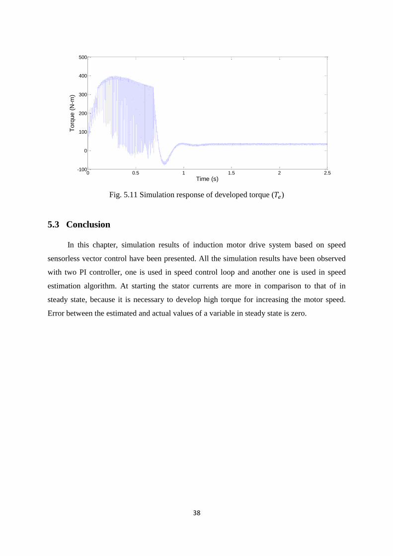
Fig. 5.11 Simulation response of developed torque (𝑇𝑒)

5.3 Conclusion

In this chapter, simulation results of induction motor drive system based on speed

sensorless vector control have been presented. All the simulation results have been observed

with two PI controller, one is used in speed control loop and another one is used in speed

estimation algorithm. At starting the stator currents are more in comparison to that of in

steady state, because it is necessary to develop high torque for increasing the motor speed.

Error between the estimated and actual values of a variable in steady state is zero.

0 0.5 1 1.5 2 2.5-100

0

100

200

300

400

500

Time (s)

Torq

ue (

N-m

)

39

Chapter-6

GENERAL CONCLUSION

6.1 Conclusion

The objective of this project was to develop a speed sensorless drive for three phase

induction motor based on a rotor flux observer. The convergence of rotor flux to reference

value is made faster by the proper selection of observer gain matrix and the speed estimation

accuracy can be improved by the observer. The speed tracking objective is achieved

succesfully and the system can operate stably in the whole operating range. The validity of

the speed tracking objective has been verified by the simulation results.

6.2 Scope for future work

The direction of future work may be divided in the following aspect:

1. The motor parameters variation was not considered through the research works.

Therefore, study the motor parameters variation in different speed, still remains

remarkable study.

2. The model of induction motor adopted here does not consider magnetic saturation.

Therefore investigation of proposed speed sensorless system in field weakening, still

remains valid in this condition.

3. It would be interesting to study the performance of sensorless vector control and to

compare it with conventional vector control.

4. The present work can be extended to estimate the rotor flux using Extended kalman

filter. A comparative study can be made with both type of flux estimators to examine

their suitability for induction motor.

40

REFERENCES

[1] H. Kubota and K. Matsuse, “Speed sensorless field-oriented control of induction

motor with rotor resistance adaptation,” IEEE Trans. Ind. App., vol. 30, no. 5, pp.

1219-1224, October 1994.

[2] R. Bojoi, P. Guglielmi and G. M. Pellegrino, “Sensorless direct field-oriented

control of three-phase induction motor drives for low-cost applications,” IEEE Trans.

Ind. Appl., vol. 44, no. 2, pp. 475-481, Mar. 2008.

[3] C. Schauder, “Adaptive speed identification for vector control of induction motor

without rotational transducers,” IEEE Trans. Ind. App., vol. 28, no. 5, pp. 1054-

1061, October 1992.

[4] B. Renukrishna and S. Shanifa Beevi, “Sensorless vector control of induction motor

drives using rotor flux observer,” 2012 IEEE International Conference on Power

Electronics, Drives and Energy Systems December 16-19, 2012, Bengaluru, India.

[5] W. Chen and D. G. Xu, “Stability analysis of speed adaptive flux observer for

induction motor speed sensorless vector control,” International Conference on

Electrical Machines and Systems, 2010.ICEMS’10, pp. 689-693, October 2010,

Incheon.

[6] G. C. Verghese and S. R. Sanders, “Observers for flux estimation in induction

machines,” IEEE Trans. Ind. Elec., vol. 35, no.1, pp. 85-94, Feb. 1998.

[7] X. Zou, P. Zhu, Y. Kang and J. Chen, “Speed Identification for speed sensorless

vector control of induction motors based on voltage decoupling control principle,”

Electrical Machines and Drives Conference, 2003.IEMDC’03. IEEE International,

vol.1, pp. 269 -273, June 2003.

[8] R. Krishnan and A.S. Bharadwaj, “A review of parameter sensitivity and adaptation

in indirect vector controlled induction motor drive systems,” Power Electronics

Specialists Conference, 1990.PESC’90, PP. 560-566, 1990.

[9] S. Tamai and H. Sugimoto, “Secondary resistance identification of an induction motor

applied model reference adaptive system and its characteristics,” IEEE Trans. Ind.

Appl., vol. 23, no. 5, pp. 296-303, march 1987.

[10] H. Kubota, I. Sato, Y. Tamura, K. Matsuse, H. Ohta, and Y. Hori, “Regenerating

mode low speed operation of sensorless induction motor drive with adaptive

41

observer”, IEEE Trans. Ind. App., vol. 38, no. 4, pp. 1081-1086, Jul./Aug. 2002.

[11] Y. R. Kim, S. K. Sul, and M. H. Park, “Speed sensorless vector control of induction

motor using extended Kalman filter,” IEEE Trans. Ind. Appl., vol. 30, no. 5, pp. 1225–

1233, Sep./Oct. 1994.

[12] M. Montanari, S. M. Peresada, C. Rossi and A. Tilli, “speed sensorless control of

induction motor based on reduced order Adaptive Observer,” IEEE Trans. Ind. Appl.,

vol. 15, no. 6, pp. 1049- 1064, Nov. 2007.

[13] B. K. Bose, “Modern Power Electronics and AC Drives,” Prentice- Hall, New Jersey,

2002.

[14] O. Barambones, A. J. Garrido and F. J. Maseda, “Integral sliding mode controller for

induction motor based on field oriented control theory,” IEEE Trans. Control Theory

Appl., vol. 1, no. 3, pp. 786- 794, May 2007.

[15] A. Sabanovic and D. B. Izosimov, “Application of sliding modes to induction motor

control,” IEEE Trans. Ind. Appl., vol. IA-17, no. 1, pp. 41–49, Jan./Feb. 1981.

[16] F. J. Lin and C. M. Liaw, “Control of indirect field-oriented induction motor drives

considering the effects of dead-time and parameter variations,” IEEE Trans. Ind.

Electronics, vol. 40, no. 5, pp. 486– 495, Oct. 1993.

[17] F. Z. Peng and T. Fukao, “Robust speed identification for speed sensorless vector

control of induction motors,” IEEE Trans. Ind. Appl., vol. 30, no. 5, pp. 1234–1240,

Sep./Oct. 1994.

[18] M. Hinkkanen and J. Luomi, “Stabilization of generating mode operation in sensorless

induction motor drives by full order flux observer design,” IEEE Trans. Ind.

Electronics, vol. 51, no. 6, pp. 1318–1328, Dec. 2004.

[19] M. Hinkkanen, “Analysis and design of full order flux observers for sensorless

induction motor ,” IEEE Trans. Ind. Appl., vol. 51, no. 5, pp. 1033- 1040, Oct. 2004.

[20] E. D. Mitronikas and A. N. Safacas, “ An improved sensorless vector control method

for an induction motor drive ,” IEEE Trans. Ind. Electronics, vol. 52, no. 6, pp. 1660-

1668, Dec. 2005.

42

APENDIX- A

Table- 2

Proportional cum Integral controller parameters

loop 𝐾𝑝 𝐾𝑖

Speed control loop 40 200

Rotor flux observer 0.05 45