Speeding up Risk Analyses of U.S. Flood Insurance … · Speeding up Risk Analyses of U.S. Flood...

Speeding up Risk Analyses of U.S. FloodInsurance Loss Data Using the Diffusion Map

Chia Ying Lee∗, Rafał Wojcik†, Charlie Wusuo Liu‡, and Jayanta Guin§

Abstract—In the insurance industry, catastrophe risk analysisusing catalogs of catastrophic events is a major componentfor quantifying financial risks of an insurance portfolios. Toensure an accurate quantification of risk, particularly for rare,strong catastrophic events, large sizes of catalogs are simulatedand used for computing loss estimates location-by-location andevent-by-event, but this is computationally intensive. In thispaper, we propose to speed up the risk computation by takinga data analytic approach to compress the catalog—specifically,using dimension reduction and clustering. To address the non-linear geometry of the loss data from the U.S. Flood model, weused a nonlinear dimension reduction technique, the diffusionmap. Combined with clustering, we show that it yields accuratecatalog compression and produces a realistic representation ofhydrometeorological patterns over the entire country. Finally,we discuss how clustering results must be refined to ensurefidelity in retaining the most important catastrophic events,and how in real life, a risk manager can utilize our results tomake informed risk management decisions.

Index Terms—Diffusion map, nonlinear dimension reduction,spectral clustering, catastrophe modeling, insurance risk ana-lytics.

I. INTRODUCTION

THE purpose of catastrophe modeling (known as CATmodelling in the industry) is to anticipate the chances

and severity of catastrophic events from earthquakes andhurricanes to terrorism and crop failure, so companies orgovernments can appropriately prepare for their financialimpact.

CAT models provide a robust, structured approach for es-timating a wide range of possible future scenario losses fromcatastrophes, along with their associated probabilities. Lossestimates produced from CAT models can be deterministicfor a specific event (e.g., Hurricane Katrina, a magnitude8.0 earthquake in San Francisco) or probabilistic from anensemble of hypothetical events [1]. The latter approach usesMonte–Carlo techniques and physical models to simulatelarge catalogs of events. For example historical data onthe frequency, location, and intensity of past hurricanes aremodeled and used to predict 10,000 catalog years of potentialhurricane experience. Each of the 10,000 years should bethought of as a potential realization from a distribution whichcharacterizes the probability of what could happen in theyear 2016, for example, instead of simulations or predictionsof hurricane activity from now until the year 12016 [2].

Manuscript received August 2, 2016; revised August 4, 2016.C. Y. Lee, C. Liu are with the Financial and Uncertainty Modeling Group,

AIR Worldwide, Boston, MA 02116 USA.R. Wojcik, is the Manager and Principal Scientist of the Financial and

Uncertainty Modeling Group, AIR Worldwide, Boston, MA 02116 USA.J. Guin is the Executive Vice President and Chief Research Officer of

Research at AIR Worldwide, Boston, MA 02116 USA.e-mail: ∗clee, †rwojcik, ‡wliu, §jguin @air-worldwide.com

To pass from catalog to financial risk, the risk analysisaggregates event losses over the locations or properties in aparticular portfolio, noting that losses are typically modeledby random variables characterized by loss distributions. Thenthe event losses are aggregated within each catalog year toobtain an aggregate annual loss (AL) distribution for eachyear. Finally, empirical samples from the overall portfolioloss distribution can be obtained from the mixture of ALdistributions. These empirical samples are used to constructthe exceedance probability (EP) curve [3], which is equiva-lent to estimating the survival function of the portfolio lossdistribution, or 1 minus its cumulative distribution function.The EP curve is the key tool used by insurers to estimatetheir probabilities of experiencing various levels of loss. Inaddition, two important risk statistics of the portfolio lossare the Average (Aggregate) Annual Loss (AAL), whichmeasures the expected AL, and the Tail Value at Risk (orp%-TVaR), which measures the expected AL conditional onobserving the upper p% tail of the portfolio loss distribution[2], [4].

Our paper is focused on the risk analysis for the U.S. floodcatalog. This catalog relies on complex, physically basedprobabilistic flood model for the U.S. [5], [6], [7], andrequires significant computational cost to estimate portfoliolosses for each flood event. This is compounded by thelarge number of events in the catalog. Therefore, it isdesirable to compress the size of the catalog to reducecomputational time. Here, we take a clustering approachto catalog compression. This idea stems from the fact thatevents in the catalog can be split into two groups: strong,infrequent events generating substantial losses and weak,frequent events generating small losses. So, we aim toidentify clusters of similar weak events in such a way that therisk analysis from the clusters provide a good approximationfor that of the full catalog. At the same time we retain allthe original strong events. Inevitably, catalog compressionwill incur errors in the portfolio’s EP curve, AAL and TVaRestimates so it is crucial to find the right patterns in the lossdata to minimize these errors.

A. Basic data set: loss matrix

The flood model for the U.S. simulates on-floodplainriverine flooding for a river network of 1.4 million miles,including all streams with a minimum drainage area of3.9 square miles, with 335,000 drainage catchments. Off-floodplain flooding is simulated only for areas away fromfloodplains [5], [7]. Each simulated flood event is charac-terized by physical model parameters, such as peak flow,peak runoff and catchments affected, from which the lossesof exposed property are calculated. Because the extent of

Proceedings of the World Congress on Engineering and Computer Science 2016 Vol I WCECS 2016, October 19-21, 2016, San Francisco, USA

ISBN: 978-988-14047-1-8 ISSN: 2078-0958 (Print); ISSN: 2078-0966 (Online)

WCECS 2016

losses depend not only on the model’s physical parametersbut also on the geomorphology of the catchments, large scaleweather patterns etc., the relationship between the physicalparameters and the losses is very complex. For this reason,we take a loss-based approach to catalog compression, inwhich industry loss data (the expected total on- and off-floodplain ground-up losses that have been estimated for allinsurable property industry-wide), is assumed to be a suitablesurrogate data set for risk analysis. The industry loss dataimplicitly reflects the physical parameters of events in thecatalog, the geomorphology of property locations and theexposure information of the properties.

Our basic data set is the loss matrix L comprising ofindustry losses in each catchment for each event,

Lij = Industry loss for event i in catchment j (1)

The dimensionality of L is huge, containing 685,477 eventscovering 335,000 catchments, but it is also sparse, becausethe majority of flood events affects only a small proportionof catchments. In practice, loss data is not always availablenationwide or at the spatial resolution of catchments. Insome data sets, the losses are aggregated to a coarser spatialresolution of zipcodes or counties. The loss data available tous are for• 6186 catchments in the Northeastern U.S.• 29911 zipcodes in the entire U.S.• 3101 counties in the entire U.S.Because the industry loss data does not contain distribu-

tional information, in this paper the portfolio loss distributionis the distribution of the means of the AL distributions. Here,the set of insurable properties within a given zipcode z istreated as a type of portfolio. Aggregating L by catalog yearsproduces Ny = 10, 000 empirical samples for the zipcodeloss distribution,

AL∗(y, z) :=∑

i:Event i ∈ Year y

Liz

Ny

y=1

.

The EP curve for that zipcode is estimated by sorting the em-pirical samples in descending order and plotting them againstthe corresponding probability. The p%-TVaR is estimated byaveraging the top p% of the empirical samples.

B. Catalog compression as clustering and multiobjectiveoptimzation

The clustering approach to the catalog compression seeksto find a clustering solution which partitions weak eventsinto disjoint subsets (clusters). Each cluster of events isthen represented by a reference event (medoid) which isan existing event within that cluster. The losses incurred byan event are approximated by that of its cluster’s referenceevent. This means that only the losses incurred by thereference event need to be computed in the risk analysis,thereby decreasing the time spent for risk computation.

Standard clustering algorithms such as k-means or hierar-chical clustering [8] are designed to minimize the differencebetween the losses of an event and its reference event.Our main objective of catalog compression is to maintainaccuracy of the EP curve and the risk statistics by minimizingerrors in the 1%-TVaR and AAL for zipcode losses:

• Average error in 1%-TVaR

FTV aR(c) =1

Nz

Nz∑z=1

∣∣∣∣TV aRc(z)− TV aR∗(z)∣∣∣∣ (2)

where TV aRc(z) is the 1%-TVaR for zipcode z com-puted under the clustering solution c, and TV aR∗(z) isthat computed from the full catalog.

• Average error in AAL

FAAL(c) =1

Nz

Nz∑z=1

∣∣∣∣∣∣ 1

Ny

Ny∑y=1

(ALc(y, z)−AL∗(y, z)

)∣∣∣∣∣∣(3)

where ALc(y, z) is annual loss of the z-th zipcode inthe y-th catalog year, under c.

In addition to the above objectives we also aim to minimizethe ratio:

Fred(c) =

∑eref

#(counties affected by reference event eref)∑e #(counties affected by event e)

(4)which counts the reduction in the number of affected countiesfor which portfolio losses need be computed. The countycompression rate 1 − Fred is closely related to the eventcompression rate, 1 − #reference events

#events . Determining the eventcompression rate is equivalent to determining the numberof clusters as in [28]. The two compression rates are notinterchangeable because of the variability in spatial extentof the clustered events: large clusters often comprise oflocalized low-loss events, while widespread high-loss eventstend to become singleton clusters. Because the actual savingsin loss computation time depend on the number of portfoliolocations for which losses need be computed and the effi-ciency with which the loss computation is implemented insoftware, the county compression rate is a preferred surrogatefor gain in computing speed.

All three criteria FTV aR,FAAL and Fred are nonlinearfunctions of the data and are not equivalent to the objectivesof standard clustering algorithms. The sole application ofthe latter may not yield an optimal solution so both sets ofobjectives should be considered as in [22] [23] and [24],[25].

Apart from the above dichotomy, (2), (3) and (4) conflictwith each other—no single clustering solution minimizesthem simultaneously. Thus, we cast the catalog compressionas Multiobjective Optimization Problem (MOP) in [21] tocompare different clustering solutions. This formalism seeksto find the Pareto front, which is the collection of Paretooptimal solutions for which no such solution is better thananother by all objectives simultaneously. (See Figure 7 fora visualization of a Pareto front). The catalog compressionproblem formulated as MOP reads:

minc∈C

(FTV aR(c),FAAL(c),Fred(c)) (MOP)

where C is the set of all possible event clustering solutions.The computational cost of the MOP can be reduced byboth using more efficient clustering algorithms and pre- orpost-processing refinements to finetune clustering solutionsas proposed [27]. For catalog compression, the refinementis targeted towards improving the accuracy of estimatingmean and tail statistics from the EP curve, by ensuring



WCECS 2016

that error-prone events become singleton clusters—clusterscomprising of a single event—thereby eliminating errors dueto approximation by a reference event.

C. The role of nonlinear dimension reduction in event clus-tering

The fundamental ingredient of any clustering technique isthe specification of a metric to quantify similarity betweendata points. Because of the ease at which Euclidean distancescan be computed, some of the most efficient clusteringalgorithms assume Euclidean metric. In high dimensional ap-plications, however, the choice of the metric is non-obviousand to large extent heuristic. Additionally, due to the curseof dimensionality [9], the concept of proximity, distanceor nearest neighbor may not be meaningful. Examples ofcounterintuitive behavior of the Minkovski norm and itsinfluence on the performance of k-means clustering are givenin [10]. To tackle the curse of dimensionality, we aim to findan embedding of the high dimensional loss matrix L ∈ RN×pinto a low-dimensional space RN×q , q p equipped withan appropriate metric (see Section III).

The well-known linear dimension reduction technique,principal component analysis (PCA), achieves this embed-ding by seeking the best low-rank approximation to identifythe best low-dimensional linear subspace that represents thedirections of greatest correlations in the data[8].The linearityof the PCA, however, limits its usefulness to situations whenthe data conform to a Gaussian assumption—an assumptionwhich our loss data does not satisfy. In fact, because ofthe sparsity of the data, the majority of events incur noloss at most zipcodes. Almost all the events lie on a nons-mooth, nonlinear manifold. In this case PCA will not givea meaningful low-dimensional representation. To tackle thisproblem, many recent techniques, including locally linearembedding [11], semidefinite embedding [12], Isomap [13],Laplacian eigenmaps [14] and the diffusion map [15], [16],[17], [18], have been proposed. One in particular, the diffu-sion map (DM), adopts the formalism of diffusion processeson a manifold in order to define a new distance (called thediffusion distance). (e.g., [19]). The DM embeds the datainto a new coordinate system that preserves the diffusiondistance such that the embedding represents the diffusiondistance within the first few eigendimensions. This makesthe DM particularly attractive to apply to the event clusteringproblem: it provides a geometry-aware distance that can beused in conjunction with Euclidean-based clustering algo-rithms. For example, [17] showed a rigorous justification fork-means clustering of the diffusion coordinates. In SectionIII we show that another clustering algorithm, the GrowingNeural Gas (GNG) [34] combined with a graph communityfinding method [33], is particularly suited to our application.In Section II we show computationally fast implementationof DM.

The paper is organized as follows. We first describe thefoundation and implementation of the DM in Section II, thengive an example of its application to the spectral clustering ofcatchments and counties into Flood Regions, in Section III.For catalog compression, Section IV-A details the main eventclustering procedure, while Section IV-B describes the pre-/post-processing refinements. We further explain the nature

Fig. 1. Intuitively, the diffusion distance reflects the connectivity by shorthops (characterized by high probability transitions) between the two endsof the arc (solid lines), in contrast to a lack of connectivity to the points inthe center (dotted line). As the diffusion time t increases, the ends of thearc grow closer, in diffusion distance, relative to their diffusion distance tothe center data points.

of the conflicting TVaR and AAL objectives in Section IV-C.Finally, in Section V, we show that the results of the overallcatalog compression methodology yields good solutions, anddemonstrate the role of Pareto optimal solutions in makingrisk management decisions.

II. DIFFUSION MAP

The DM constructs a nonlinear transformation of high-dimensional data into the diffusion space, through a spectraldecomposition of the graph Laplacian, defined by a randomwalk on the graph of data points that respects the connec-tivity and topological structure of the data manifold. Suchdecomposition provides an efficient representation of the datain terms of the diffusion coordinates, the leading few ofwhich are used to define a low dimensional embedding ofthe data. In what follows, we give the theoretical frameworkand discuss computationally fast implementation of the DM.

A. Theory

The input to the DM is a symmetric weight matrix W ,where Wij > 0 represents similarity between data pointsxi, xj . Then, the algorithm constructs a Markov random walkon the weighted graph G = (X,W ), with transition matrixP given by

Pij =Wij

di, (5)

where di =∑kWik is the degree of vertex xi. Under the

positivity condition of Wij and if G is connected, the randomwalk converges to a unique stationary distribution,

limt→∞

P(t)ij =

dj∑k dk

:= φ∗j . (6)

where P (t) = P t is the t-step transition matrix. Therandom walk favors transitions between similar points, so thestationary distribution concentrates in regions of high datadensity. The diffusion distance D(t), at a diffusion time t,reflects the connectivity by short and highly probable pathsbetween two data points xi, xj (see Fig. 1). This gives riseto its probabilistic definition, which can be re-expressed ina more convenient form in terms of the eigendecomposition



WCECS 2016

Algorithm 1: DM algorithm.

Input : Weight matrix W (derived from data X ∈ RN×m),maximum embedding dimension pmax.

1 d← rowSums(W) // vertex degrees2 φ∗ ← d/sum(d) // stationary distribution3 ∆← diag(d−1/2).4 W ← ∆ ∗W ∗∆ // symmetric graph Laplacian

5 (Λ, V )← eigendecomposition(W , pmax)6 (t, p)←getTimeDimension(Λ) // (see text)7 ψ ← ∆ ∗ V [:, 1:p] // right eigenvector8 ψ ← ψ∗diag((t(φ∗)∗ψ)ˆ−1/2) // normalize9 Ψ← ψ∗diag(Λ[1:p]ˆt) // diffusion coordinates

Output: Diffusion coordinates Ψ ∈ RN×p.

of the transition matrix:

(D(t)ij )2 :=

∑k

(P(t)ik − P

(t)jk )2

φ∗k≡N−1∑k=0

λ2tk (ψik − ψjk)2

(7)

where λk, ψ·,k are the eigenvalues and corresponding righteigenvector of P (normalized w.r.t. the weight φ∗). Notethat λ0 = 1 and ψ·,0 ≡ 1 is a constant vector. If theeigenvalues decay sufficiently fast, the summation in Eq.7 can be approximated by the first p summands, chosenup to error tolerance. By defining the diffusion map—thetransformation of the data points into the p-dimensionaldiffusion space—as

Ψ(t) : xi ∈ RN 7→ (λt1ψi1, . . . , λtpψip)

T ∈ Rp, (8)

it follows that the diffusion distance is approximated by theEuclidean distance of the diffusion coordinates,

(D(t)ij )2 ≈ ‖Ψ(t)(xi)−Ψ(t)(xj)‖2. (9)

B. Algorithm and Implementation

Given an input similarity measure Sim(·, ·), a commonchoice for the weight matrix W is to use a Gaussian kernel,

Wij = e−(1−Sim(xi,xj))2/2κ2

.

The kernel width, κ, can be automatically set as the mediandistance of each data point’s k-th nearest neighbor [18], withk typically 1% of the data size. The diffusion time t andembedding dimension p should meet an error tolerance forthe approximation of D(t); e.g. to satisfy p = maxj : |λtj | >δ|λt1| for a given tolerance δ [17]. In practice, we chooseδ = 0.1 and fix a maximum dimension pmax (to limit thenumber of eigenvectors that must be computed), and thenchoose t large enough to meet the error tolerance.

Algorithm 1 shows the basic steps of DM implementation.It uses the symmetric graph Laplacian in lieu of the transitionmatrix, so that eigendecomposition for symmetric matricescan be used. This step is often the computational bottleneckwith large data, but we the fast randomized SVD techniqueof [29] can tackle this problem. Our implementation of theDM algorithm in R/Rcpp is as follows:• Fast linear algebra using fast randomized SVD algo-

rithm [29]. Based on a random projection and iterativeorthogonalization procedure, the fast randomized SVDalgorithm reduces the estimation of the leading singularvalues to the eigendecomposition of a small matrix.

Algorithm 2: Fast randomized eigendecomposition of sym-metric matrices, with power iteration [29, Algorithms 4.4 and5.3].

Input : Symmetric matrix A ∈ Rn×n, desired number ofeigendimensions p, and number of power iterationsq.

1 Ω← rnorm(n, 2p); // random Gaussian matrix2 for i← 0 to 2q do3 (Q,R)←qr(A ∗ Ω); // QR decomposition4 Ω← Q;5 end6 B ← transpose(Ω) ∗A ∗ Ω; // a small matrix7 (Λ, V )← eigen(B); // eigendecomposition8 Λ← Λ[1:p]; V ← V [,1:p];

Output: Eigenvalues Λ ∈ Rp, eigenvectors V ∈ Rn×p.

The random projection is justified by the Johnson-Linderstrauss lemma [30]. We used a version for eigen-decomposition of symmetric matrices (shown in Algo-rithm 2) with complexity O((q + 1)(N2p+Np2)).

• Memory efficient implementation requiring negligibleadditional memory allocation. Memory efficiency isachieved by utilizing packed storage of symmetric ma-trices [31] and designing modification-in-place subrou-tines.

• Optimized BLAS libraries for symmetric packed matrixmultiplication. In Algorithm 2, the multiplication ofthe (large) input matrix with the (small) random Gaus-sian matrix is performed by the BLAS routine dspmv[31] for symmetric packed matrix-vector multiplication.Note that if the input matrix is too large to fit intoRAM, a single-pass matrix multiplication scheme canbe adopted to allow entry-wise streaming of the inputmatrix.

• Higher eigendecomposition accuracy possible with ad-ditional computation. The option to improve the ap-proximation accuracy utilizes a power iteration featureof the fast randomized eigendecomposition algorithm.The additional cost is due to multiple repetitions ofmatrix multiplication. Empirically, q = 2 is sufficientfor accurate results.

• Speed up with parallelization. Many of the computa-tions are highly parallelizable.

III. AN EXAMPLE: SPECTRAL CLUSTERING OF FLOODREGIONS USING DM

In this section we illustrate the efficacy of the DM usingan example of clustering catchments or counties, insteadof events, into regions of similar flood activity. To clustercatchments, the loss matrix is transposed, L′, so that eachdata point z ∈ RN represents a catchment’s losses fromthe N events in the catalog. The input to the DM can beany similarity measure computed on L′ (e.g. Jaccard andYule similarities, Simple Matching Coefficient, correlationcoefficient, Euclidean distance, etc.), so that it defines acorresponding diffusion distance. Thereafter, a clustering al-gorithm is applied to the Euclidean distance on the diffusioncoordinates, noting that conceptually, it is the closeness withrespect to the diffusion distance that the clusters obey. Thisis illustrated in Figure 2.



WCECS 2016

Fig. 2. Workflow for spectral clustering using DM. In parentheses areballpark computational times taken on the Northeastern U.S. catchmentloss data set, computed on a 3.4 GHz Intel i7-4770 processor. Our DMimplementation used 8 core parallelization; the other algorithms used asingle core. GNG+GCF used the gmum.r package [32].

As mentioned before, clustering algorithms that require anEuclidean distance assumption (such as k-means, neural gas),as well as those that accept an arbitrary similarity measure(such as hierarchical clustering, agnes) can now be used. An-other clustering method that is particularly effective for thisapplication is the Growing Neural Gas algorithm combinedwith a graph community finding algorithm (GNG+GCF):• The Growing Neural Gas (GNG) algorithm combines

key ideas from competitive Hebbian learning and theNeural Gas algorithm to build a graph of nodes thatrepresent the centroids of clusters, defined through theVoronoi tesselation. An edge between two nodes reflectsthe density of data points connecting the nodes.

• Graph community finding (GCF) algorithms attempt tofind communities of nodes that are highly connectedwithin each community but poorly connected withother communities. One way communities are foundis through minimizing the modularity score function,which measures the fraction of edges falling within acommunity: ∑

n,n′ En,n′δcn,cn′∑n,n′ En,n′

where edge En,n′ = 1 if nodes n, n′ are connected,and 0 otherwise; cn is the community to which nbelongs. GCF is achieved by the fast greedy modularityoptimization algorithm [35], which is of almost linearcomplexity, O(n log2 n). A drawback of GCF is thatthe exact number of communities is not known a priori.

To obtain effective clustering using GNG+GCF, the GNGwas trained using more nodes than the number of desiredregions, so that each node represents a “micro-cluster” ofcatchments. Then, a flood region is formed by a communityof nodes found by the GCF algorithm, which represents thecorresponding collection of catchments.

For catchment loss data in Northeastern U.S., we per-formed the spectral clustering using DM as shown in Figure2. In our experiments, the Jaccard similarity yielded the bestresults. It is defined as

SimJac(z, z′) :=

n11n11 + n10 + n01

,

where the entries of the data points z, z′ are first converted tobinary values (with 1 and 0 indicating positive and zero loss,respectively), and then nij = |k : zk = i and z′k = j|.

Fig. 3. Map of Northeastern U.S. catchments clustered into six regions,using the benchmark method (LEFT) and GNG+GCF clustering on thediffusion distance (RIGHT). Catchments not affected by any event are notincluded.

Fig. 4. 3D visualization of the first 3 diffusion coordinates, for diffusiontime t = 5 and dimension p = 4. The GNG+GCF algorithm was used with200 nodes. The labeled groups of nodes correspond to the Regions B andC in Figure 3 RIGHT

The Jaccard similarity computes overlap ratios and is well-suited to image and text processing applications [36]. Here,two catchments are Jaccard-similar if the events affectingboth catchments form a large proportion of those affectingat least one of the catchments; that is, if they have a similarpropensity for flooding.

We looked for heuristic qualities of how well hiddenrelationships in the data were captured, such as the abil-ity to reproduce large scale weather patterns and maintaingeographical connectivity of the regions. For comparison,hierarchical clustering based on the correlation coefficientCorr(z, z′) = V ar(z, z′)/

√V ar(z)V ar(z′), a method used

in feature cluster analysis, was used as a benchmark.• The methods shown in Figure 2 and the benchmark

method produced regions with fairly cohesive bound-aries, and broadly captured weather patterns moving ina northeastern direction.

• Hierarchical and k-means clustering on the diffusiondistance, as well as the benchmark method, were unableto separate the two coastal regions that are subjectedto the same weather patterns but are geographicallydisconnected. (Region A in Figure 3 LEFT.)

• Only GNG+GCF clustering on the diffusion distancesuccessfully distinguished the two geographically sepa-rated coastal regions (Regions B, C in Figure 3 RIGHT)

• The DM provides a visualization of the catchments withsimilar weather patterns, particularly the ‘closeness’ ofthe separate coastal regions (Figure 4). This explainswhy it is easy for a clustering algorithm to cluster



WCECS 2016

those two regions together. Nonetheless, GNG+GCFdistinguishes those two regions because the correspond-ing groups of nodes are sparsely interconnected despitebeing close in diffusion distance.

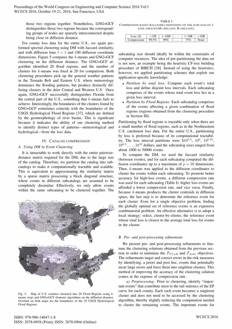
For county loss data for the entire U.S., we again per-formed spectral clustering using DM with Jaccard similarity,and with diffusion time t = 1 and 100 diffusion coordinatedimensions. Figure 5 compares the k-means and GNG+GCFclustering on the diffusion distance. The GNG+GCF al-gorithm identified 20 flood regions, and the number ofclusters for k-means was fixed at 20 for comparison. Bothclustering procedures pick up the general weather patternsin the Tornado Belt and Eastern U.S. where meteorologydominates the flooding patterns, but produce distinctly dif-fering clusters in the drier Central and Western U.S. Onceagain, GNG+GCF successfully distinguishes Florida fromthe central part of the U.S., something that k-means fails toachieve. Interestingly, the boundaries of the clusters found byGNG+GCF sometimes coincide with the boundaries of theUSGS Hydrological Flood Regions [37], which are definedby the geomorphology of river basins. This is significantbecause it indicates the ability of our clustering methodto identify distinct types of patterns—meteorological andhydrological—from the loss data.

IV. CATALOG COMPRESSION

A. Using DM in Event Clustering

It is intractable to work directly with the entire pairwise-distance matrix required for the DM, due to the large sizeof the catalog. Therefore, we partition the catalog into sub-catalogs to make it computationally tractable and scalable.This is equivalent to approximating the similarity matrixby a sparse matrix possessing a block diagonal structure,where events in different subcatalogs are assumed to becompletely dissimilar. Effectively, we only allow eventswithin the same subcatalog to be clustered together. The

Fig. 5. Map of U.S. counties clustered into 20 Flood Regions using k-means (top) and GNG+GCF (bottom) algorithms on the diffusion distance.Overlaid on both maps are the boundaries of the 18 USGS HydrologicalFlood Regions.

TABLE ICOMPRESSION RATES (BALLPARK) DEPENDING ON THE SUBCATALOG’S

LOSS AMOUNT(M=MILLION, B=BILLION).

Loss ($) <1M 1–10M . . . 1–10B >10BCompression 99.5% 99% . . . 75% None

subcatalog size should ideally be within the constraints ofcomputer resources. The idea of pre-partitioning the data setis not new, an example being the heuristic CF-tree buildingprocedure of BIRCH [38]. Instead of using the heuristics,however, we applied partitioning schemes that exploit ourapplication-specific knowledge:• Partition by total loss: Compute each event’s total

loss and define disjoint loss intervals. Each subcatalogcomprises of the events whose total event loss lies in agiven loss interval.

• Partition by Flood Regions: Each subcatalog comprisesof the events affecting a given combination of floodregions (regions obtained from the clustering procedurein Section III).

Partitioning by flood regions is tractable only when there area small number of flood regions, such as in the NortheasternU.S. catchment loss data. For the entire U.S., partitioningby loss is preferred because of its computational tractabil-ity. The loss interval partitions were $105.5, 106, 106.25,106.5, . . . , 1010 dollars, and the subcatalog sizes ranged fromabout 1000 to 50000 events.

To compute the DM, we used the Jaccard similarity(between events), and for each subcatalog computed the dif-fusion coordinates up to a maximum of p = 50 dimensions.Then, k-means was applied to the diffusion coordinates tocluster the events within each subcatalog. To promote betteraccuracy for high-loss events, a different compression ratewas used for each subcatalog (Table I): higher loss events areafforded a lower compression rate, and vice versa. Finally,because k-means produces the cluster centroids in diffusionspace, the last step is to determine the reference event foreach cluster. Even for a single objective problem, findingthe globally optimal set of reference events is an expensivecombinatorial problem. An effective alternative is to adopt alocal strategy: select, cluster-by-cluster, the reference eventwhose total loss is closest to the average total loss for eventsin the cluster.

B. Pre- and post-processing refinements

We present pre- and post-processing refinements to fine-tune the clustering solutions obtained from the previous sec-tion in order to minimize the FTV aR and FAAL objectives.The refinements target and correct errors in the risk measuresby identifying, a priori and post hoc, events that potentiallyincur large errors and force them into singleton clusters. Thismethod of improving the accuracy of the clustering solutioncomes at the expense of compression rate.

a) Preprocessing: Prior to clustering, identify “impor-tant events” that contribute most to the tail statistics of the EPcurve for each county. Each such event becomes a singletoncluster and does not need to be accessed by the clusteringalgorithm, thereby slightly reducing the computation neededto cluster the remaining events. The important events for



WCECS 2016

Algorithm 3: Extremal Error Correction for TVaR.The zipcodes are handled in the order of their error’s magnitude. For each

zipcode, the order in which events in the top 100 years (which factor

into the 1%-TVaR computation) are converted to singleton clusters depends

on whether the TVaR was under- or over-estimated; in the former, events

incurring the most negative errors go first. This minimizes the number of

additional singleton clusters. The process is iterated until all errors are within

the threshold.Input : Error threshold ε, loss matrix L, clustered loss matrix M .

1 zErrors ← computeErrors(L,M);2 while max(|zErrors|) > ε do3 zRank ← argsort(−zErrors); // decreasing4 for z in zRank do5 if zErrors[z] < −ε then // underestimation6 eRank ← argsort(M [:, z]− L[:, z]);7 else8 eRank ← argsort(L[:, z]−M [:, z]);9 end

10 i ← 0;11 while |zErrors[z]| > ε do12 e← eRank[i]; i← i + 1;13 topYears←computeTopYears(M [:, z]);14 if Year(e) ∈ topYears then

// Convert event e to singleton15 M [e, z]← L[e, z];16 zErrors[z]←updateError(L[:, z],M [:, z]);17 end18 end19 end20 zErrors ← computeErrors(L,M);21 end

Output: New clustering solution.

each county are those that make up at least 95% of its 1%-TVaR estimate, as well as those that make up 50% of its1.5%-TVaR estimate. The union of important events for allcounties is the overall important event set, and comprises16.5% of the catalog.

b) Postprocessing: Upon obtaining a clustering solu-tion, identify the events that contribute most to the TVaR orAAL error, and convert them to singleton clusters. This pro-cess necessarily decreases the compression rate. We proposethe Extreme Error Correction algorithm to perform this re-finement, given a desired error threshold. Algorithm 3 showsthe algorithm for correcting TVaR errors; the algorithm forAAL is similar.

C. Conflicting TVaR and AAL objectives

It is intuitive that FTV aR and Fred are conflicting ob-jectives, but it is less obvious that the two error metricsFTV aR and FAAL conflict. The reason for this conflict isbest illustrated by an extreme example: if in a clusteringsolution, the important TVaR events are each turned intosingleton clusters, and all remaining events form one hugecluster, then one would expect a very good FTV aR but verybad FAAL. The act of re-allocating singleton clusters towardsmaintaining accuracy of important TVaR events, withoutchanging the compression rate, comes at the expense ofaccuracy for other events and hence at the expense of AALerror.

This trade-off between the two objectives is shown inFigure 6, where the NSGA2 algorithm [26] was used toestimate the Pareto front for the bi-objective optimizationof FTV aR,FAAL. The population size was 200, and apenalty on the event compression rate was imposed on the

Fig. 6. Estimated (1st) Pareto front in 2-objective space (black). The othersolutions are ranked by their closeness to Pareto optimality: the 2nd frontbecomes the new estimated Pareto front if the 1st front is removed; the r-thfront becomes the estimated Pareto front if all fronts ranked less than r areremoved. All solutions have approximately 74.3% event compression rate.

Fig. 7. Estimated Pareto fronts for 3-objective space. On the z-axis is thereduction rate Fred. Note that the error objectives shown are the averagerelative errors, instead of the average absolute errors in (2), (3).

fitness function. For the genetic operators in NSGA2, themutation operator was designed to randomly split or mergeclusters. The solutions shown in Figure 6 have roughly thesame event compression rate of 74.3%. However, while theFTV aR,FAAL trade-off is interesting and subtle, the trade-off with Fred is more significant.

V. SIMULATION RESULTS

We ran the catalog compression methodology on the 10KU.S. flood catalog, using industry loss data at the countyand zipcode resolutions. A collection of candidate solutionswas obtained by running the full methodology with varyingpre- and post-refinement parameters, to yield 162 solutionswith county compression rates ranging from 40-70%. Figure7 shows the candidate solutions in 3D-objective space, in-cluding the estimated Pareto optimal solutions in black. Weobserve a trade off between the three objectives, but the mostsignificant trade off is between the 1%-TVaR (or AAL) errorand the reduction ratio Fred.

At this juncture, a risk manager is enlisted to select thefinal solution, based on a desired accuracy, compression



WCECS 2016

Fig. 8. Estimated Pareto fronts in 2-objective space using TVaR errors forzipcodes and portfolio locations.

rate or other managerial criteria. A typical decision makingprocess may proceed as follows.

Suppose the risk manager desires a county compressionrate of at least 60%, and he also has a portfolio of 800insured locations on the East coast of the U.S. He isconcerned with the average TVaR errors for both zipcodesnationwide and in his portfolio, but is willing to acceptmore error in his portfolio than nationwide, up to 5% error.He looks at the Pareto optimal solutions subject to thiscriteria (Figure 8), and selects the one with an acceptablelevel of error: 2.4% error nationwide, and 3.8% error inhis portfolio. This solution has 75.1% event compressionrate and 60.1% county compression rate, and is producedafter the sequential application of extreme error correctionto the event clustering solution at the zipcode resolutionwith a threshold of 10% error in TVaR and 15% error inAAL. To ensure good results at the county resolution, hefurther passes the selected solution through a final touch-upusing extreme error correction at the county resolution witha threshold of 5% error in TVaR and 10% error in AAL. Thefinal solution has 74.9% event compression rate and 59.9%county compression rate. The resulting errors of the finalcompressed catalog, at the county resolution, are shown inFigure 9. Figure 10 shows a good agreement between the EPcurves estimated from the full and the clustered catalogs.

VI. CONCLUSION

We showed the application of the DM for dimensionreduction and spectral clustering in the context of U.S. floodinsurance risk analysis. By applying event clustering in con-junction with a refinement strategy to optimize the estimationaccuracy of the risk measures, we can compress the catalogsize to speed up loss computation. We showed that even atevent compression rates close to 75%, a high accuracy inrisk measures is maintained. Risk management decisions areaided by the presentation of Pareto optimal solutions underthe multiobjective optimization framework.

This entire methodology of combining general dimensionreduction and clustering techniques with problem specificoptimization and refinement algorithms can be useful inmany other applications. Furthermore, the low dimensionalembedding produced by the DM provides a good visualiza-tion of the relationships between catchments or counties (ormore generally, spatial dimensions). By using an appropriate

Fig. 9. Map of the U.S. showing 1%-TVaR and AAL errors by county.

0.000 0.004 0.008

120

180

240

0.000 0.004 0.008

120

180

240

County #1

Error: 4.57% (AAL); 2.21% (1%−TVAR)Exceedance probability

Loss

($M

) FullClustered

0.000 0.004 0.008

300

500

700

0.000 0.004 0.008

300

500

700

County #2


Loss

($M

) FullClustered

0.000 0.004 0.008

1000

4000

7000

0.000 0.004 0.008

1000

4000

7000

County #3


Loss

($M

) FullClustered

0.000 0.004 0.008

500

1500

2500

0.000 0.004 0.008

500

1500

2500

County #4


Loss

($M

) FullClustered

0.000 0.004 0.008

100

250

400

0.000 0.004 0.008

100

250

400

County #5


Loss

($M

) FullClustered

0.000 0.004 0.008

1520

25

0.000 0.004 0.008

1520

25

County #6


Loss

($M

) FullClustered

0.000 0.004 0.008

800

1200

0.000 0.004 0.008

800

1200

County #7


Loss

($M

) FullClustered

0.000 0.004 0.008

100

200

0.000 0.004 0.008

100

200

County #8


Loss

($M

) FullClustered

Fig. 10. EP curves constructed from the full and clustered catalogs, forselected counties, including some with the highest errors.

clustering algorithm, such as GNG+GCF, this clusteringmethodology is better able to reveal hidden relationships inthe data, as illustrated by the weather patterns and geograph-ical connectivity captured in the U.S. county loss data.



WCECS 2016

ACKNOWLEDGMENT

The authors would like to thank Dan Reese and RaulinaWojtkiewicz for their assistance with acquiring the data sets.

REFERENCES

[1] K. Clark, “Catastrophe risk,” in IAA Risk Book – Governance, Manage-ment and Regulation of Insurance Operations. International ActuarialAssociation / Association Actuarielle Internationale, 2015.

[2] S. Latchman, “Quantifying the risk of natural catastrophes,” 2010.[Online]. Available: http://understandinguncertainty.org/node/622

[3] P. Grossi, H. Kunreuther, and D. Windeler, “An introduction tocatastrophe models and insurance,” in Catastrophe modeling: a newapproach to managing risk, ser. Huebner International Series on Risk,Insurance and Economic Security, G. Patricia and H. Kunreuther, Eds.Springer Science+Business Media, 2005.

[4] P. Artzner, F. Delbaen, J.-M. Eber, and D. Heath, “Coherent measuresof risk,” Mathematical Finance, vol. 9, no. 3, pp. 203–228, 1999.

[5] B. Dodov and A. Weiner, “Introducing the AIR inland flood modelfor the United States,” 2013. [Online]. Available: http://www.air-worldwide.com/Publications/AIR-Currents/2013/Introducing-the-AIR-Inland-Flood-Model-for-the-United-States/

[6] R. Wojtkiewicz, J. Rollins, and V. Foley, “U.S. flood insurance - theNFIP and beyond,” http://www.air-worldwide.com/Publications/AIR-Currents/2013/U-S–Flood-Insurance%E2%80%94the-NFIP-and-Beyond/, , 2013.

[7] AIR-WORLDWIDE, “The AIR inland flood model forthe United States,” Brochure, 2013. [Online]. Available:http://www.air-worldwide.com/publications/brochures/documents/air-inland-flood-model-for-the-united-states/

[8] T. Hastie, R. Tibshirani, and J. Friedman, The elements of statisticallearning, 2nd ed., ser. Springer Series in Statistics. Springer, NewYork, 2009.

[9] R. Bellman, Dynamic Programming, 1st ed. Princeton, NJ, USA:Princeton University Press, 1957.

[10] C. C. Aggarwal, A. Hinneburg, and D. A. Keim, Database Theory —ICDT 2001: 8th International Conference London, UK, January 4–6,2001 Proceedings. Berlin, Heidelberg: Springer Berlin Heidelberg,2001, ch. On the Surprising Behavior of Distance Metrics in HighDimensional Space, pp. 420–434.

[11] S. T. Roweis and L. K. Saul, “Nonlinear dimensionality reduction bylocally linear embedding,” Science, vol. 290, no. 5500, pp. 2323–2326,2000.

[12] K. Q. Weinberger and L. K. Saul, “Unsupervised learning of imagemanifolds by semidefinite programming,” in Proceedings of the 2004IEEE Computer Society Conference on Computer Vision and PatternRecognition, vol. 2, June 2004, pp. II–988–II–995 Vol.2.

[13] J. B. Tenenbaum, V. d. Silva, and J. C. Langford, “A global geometricframework for nonlinear dimensionality reduction,” Science, vol. 290,no. 5500, pp. 2319–2323, 2000.

[14] M. Belkin and P. Niyogi, “Laplacian eigenmaps for dimensionalityreduction and data representation,” Neural Computation, vol. 15, pp.1373–1396, 2003.

[15] R. R. Coifman and S. Lafon, “Diffusion maps,” Appl. Comput.Harmon. Anal., vol. 21, no. 1, pp. 5–30, 2006.

[16] S. Lafon, Y. Keller, and R. R. Coifman, “Data fusion and multicuedata matching by diffusion maps,” IEEE Trans. Pattern Anal. Mach.Intell., vol. 28, no. 11, pp. 1784–1797, Nov 2006.

[17] S. Lafon and A. Lee, “Diffusion maps and coarse-graining: a unifiedframework for dimensionality reduction, graph partitioning, and dataset parameterization,” IEEE Trans. Pattern Anal. Mach. Intell., vol. 28,no. 9, pp. 1393–1403, Sept 2006.

[18] A. B. Lee and L. Wasserman, “Spectral connectivity analysis,” J. Amer.Statist. Assoc., vol. 105, no. 491, pp. 1241–1255, 2010.

[19] R. Talmon, I. Cohen, S. Gannot, and R. R. Coifman, “Diffusion mapsfor signal processing: A deeper look at manifold-learning techniquesbased on kernels and graphs,” IEEE Signal Process. Mag., vol. 30,no. 4, pp. 75–86, July 2013.

[20] J. Shi and J. Malik, “Normalized cuts and image segmentation,” IEEETrans. Pattern Anal. Mach. Intell., vol. 22, no. 8, pp. 888–905, Aug.2000.

[21] C. A. Coello Coello, G. B. Lamont, and D. A. Van Veldhuizen, Evo-lutionary Algorithms for Solving Multi-Objective Problems. Spring-Verlag New York Inc., 2007.

[22] L. Kaufman and P. Rousseeuw, Finding Groups in Data: An Introduc-tion to Cluster Analysis, ser. Wiley Series in Probability and Statistics.Wiley, 2005.

[23] R. T. Ng and J. Han, “CLARANS: a method for clustering objects forspatial data mining,” IEEE Trans. Knowl. Data Eng., vol. 14, no. 5,pp. 1003–1016, Sep 2002.

[24] U. Maulik and S. Bandyopadhyay, “Genetic algorithm-based clusteringtechnique,” Pattern Recognition, vol. 33, pp. 1455–1465, 2000.

[25] L. Agustin-Blas, S. Salcedo-Sanz, S. Jimenez-Fernandez, L. Carro-Calvo, J. Del Ser, and J. Portilla-Figueras, “A new grouping geneticalgorithm for clustering problems,” Expert Syst. Appl., vol. 39, no. 10,pp. 9695–9703, Aug. 2012.

[26] K. Deb, A. Pratap, S. Agarwal, and T. Meyarivan, “A fast and elitistmultiobjective genetic algorithm: Nsga-ii,” IEEE Trans. Evol. Comput.,vol. 6, no. 2, pp. 182–197, Apr 2002.

[27] I. S. Dhillon, Y. Guan, and J. Kogan, “Iterative clustering of high di-mensional text data augmented by local search,” in IEEE InternationalConference on Data Mining (ICDM), dec 2002.

[28] G. W. Milligan and M. C. Cooper, “An examination of proceduresfor determining the number of clusters in a data set,” Psychometrika,vol. 50, no. 2, pp. 159–179, 1985.

[29] N. Halko, P. G. Martinsson, and J. A. Tropp, “Finding structure withrandomness: probabilistic algorithms for constructing approximatematrix decompositions,” SIAM Rev., vol. 53, no. 2, pp. 217–288, 2011.

[30] S. Dasgupta and A. Gupta, “An elementary proof of the Johnson-Lindenstrauss lemma,” Tech. Rep., 1999.

[31] E. Anderson, Z. Bai, C. Bischof, S. Blackford, J. Dongarra, J. Du Croz,A. Greenbaum, S. Hammarling, A. McKenney, and D. Sorensen,LAPACK Users’ Guide: Third Edition. Society for Industrial andApplied Mathematics, 1999.

[32] W. Czarnecki, S. Jastrzebski, M. Data, I. Sieradzki, M. Bruno-Kaminski, K. Jurek, P. Kowenzowski, M. Pletty, K. Talik, andM. Zgliczynski, gmum.r: GMUM Machine Learning Group Package,2015. [Online]. Available: https://github.com/gmum/gmum.r

[33] I. T. Podolak and S. K. Jastrzebski, Proceedings of the 8th In-ternational Conference on Computer Recognition Systems CORES2013. Springer International Publishing, 2013, ch. Density InvariantDetection of Osteoporosis Using Growing Neural Gas, pp. 629–638.

[34] B. Fritzke, “A growing neural gas network learns topologies,” inAdvances in Neural Information Processing Systems 7. MIT Press,1995, pp. 625–632.

[35] A. Clauset, M. E. J. Newman, and C. Moore, “Finding communitystructure in very large networks,” Physical review. E, Statistical,nonlinear, and soft matter physics (Print), vol. 70, no. 6 Part 2, p.066111, Dec 2004.

[36] J. Leskovec, A. Rajaraman, and J. D. Ullman, Mining of MassiveDatasets, 2nd ed. Cambridge University Press, 2014.

[37] U. S. Geological Survey and U. S. Department of Agricultureand Natural Resources Conservation Service, Federal Standards andProcedures for the National Watershed Boundary Dataset (WBD),2013. [Online]. Available: http://pubs.usgs.gov/tm/11/a3/

[38] T. Zhang, R. Ramakrishnan, and M. Livny, “BIRCH: An efficient dataclustering method for very large databases,” SIGMOD Rec., vol. 25,no. 2, pp. 103–114, Jun. 1996.



WCECS 2016

Date post:	17-Aug-2018
Category:	Documents
Upload:	letu
View:	214 times
Download:	0 times

Speeding up Risk Analyses of U.S. Flood Insurance … · Speeding up Risk Analyses of U.S. Flood...

Documents