SPHERE-ZIMPOL system testing: status report on polarimetric high contrast results

Ronald Roelfsema*a, Daniel Gislerb, Johan Pragta, Hans Martin Schmidb, Andreas Bazzonb, Carsten Dominikj, Andrea Baruffoloc, Anthony Boccalettie, Jean-Luc Beuzitd, Anne Costilleg, Kjetil Dohleng,

Mark Downingf, Eddy Elswijka, Menno de Haana, Norbert Hubinf, Markus Kasperf, Christoph Kellerl, Matthew Kenworthyl, Jean-Louis Lizonf, Patrice Martinezd, David Mouilletd, Alexey

Pavlovh, Pascal Pugetd, Bernardo Salasnichc, Jean-Francois Sauvagem, Christian Thalmannj, Francois Wildik

aNOVA-ASTRON, Oude Hoogeveensedijk 4, 7991 PD Dwingeloo, The Netherlands; bInstitute of Astronomy, ETH Zurich, 8093 Zurich, Switzerland; cINAF, Osservatorio Astronomico di Padova, 35122 Padova, Italy; dIPAG, Université Joseph Fourier, BP 53, 38041 Grenoble cedex 9, France;

eLESIA, Observatoire de Paris, 5 place J. Janssen, 92195 Meudon, France; fESO, Karl-Schwarzschild-Strasse 2, D-85748 Garching bei München, Germany; gLAM, UMR6110, CNRS/Universite de Provence, 13388 Marseille cedex 13, France; hMax-Planck-Institut fur Astronomie, Königstuhl 17, 69117 Heidelberg, Germany; jAstronomical Institute “Anton

Pannekoek”, 1098 SJ Amsterdam, The Netherlands; kObservatoire Astronomique de l’Universite de Geneve, 1290 Sauverny, Switzerland; lLeiden Observatory, Niels Bohrweg 2, P.O. Box 9513, 2300

RA Leiden, The Netherlands; mONERA, BP 72, 92322 Chatillon France

ABSTRACT

SPHERE (Spectro-Polarimetric High Contrast Exoplanet Research) is one of the first instruments which aim for the direct detection from extra-solar planets. SPHERE commissioning is foreseen in 2013 on the VLT. ZIMPOL (Zurich Imaging Polarimeter) is the high contrast imaging polarimeter subsystem of the ESO SPHERE instrument. ZIMPOL is dedicated to detect the very faint reflected and hence polarized visible light (600-900 nm) from extrasolar planets. It is located behind an extreme AO system (SAXO) and a stellar coronagraph. We present the first high contrast polarimetric results obtained for the fully integrated SPHERE-ZIMPOL system. We have measured the polarimetric high contrast performance of several coronagraphs: a Classical Lyot on substrate, a suspended Classical Lyot and two 4 Quadrant Phase Mask coronagraphs. We describe the impact of crucial system parameters – Adaptive Optics, Coronagraphy and Polarimetry - on the contrast performance. Keywords: SPHERE, ZIMPOL, High Contrast, Exo Planets, Polarimetry, Adaptive Optics, Coronagraphy

1. INTRODUCTION

SPHERE-ZIMPOL1,2,3 (Spectro-Polarimetric High Contrast Exoplanet Research - Zurich Imaging Polarimeter) is one of the first instruments which aim for the direct detection of reflected light from extra-solar planets. The instrument will search for direct light from old planets with orbital periods of a few months to a few years as we know them from our solar system. These are planets which are in or close to the habitable zone.

The reflected radiation is generally polarized4,5 and the degree of polarization may be particularly high at short wavelengths < 1μm due to Rayleigh scattering by molecules and scattering by haze particles in planetary atmospheres. For this reason the visual-red spectral region is well suited for planet polarimetry.

*roelfsema@astron.nl; phone +31-(0)521-595172

The search for reflected light from extra-solar planets is very demanding, because the signal decreases rapidly with the orbital separation a. For a Jupiter-sized object and a separation of 1 AU the planet/star contrast to be achieved is on the order of 10-8 for a successful detection6. This is much more demanding than the direct imaging of young self-luminous planets.

Therefore SPHERE-ZIMPOL will be capable to investigate only the very nearest stars for the polarization signal from extra-solar planets. There are half a dozen of good candidate systems for which giant planets should be detectable, even if their properties are not ideal (low albedo, not highly polarized). In another handful targets there is some chance to find high-polarization planets, if they exist around them. For stars further away a detection of reflected light with SPHERE-ZIMPOL will be difficult.

At the present moment only two instruments at 8 meter class telescopes provide high angular resolution polarimetric capabilities in the near InfraRed: NAOS-CONICA7 on the VLT and HiCIAO8 on Subuaru. SPHERE-ZIMPOL will be unique for providing high angular resolution polarimetry in the visible.

In this paper we present the first high contrast polarimetric results obtained for the fully integrated SPHERE-ZIMPOL system and we describe the impact of crucial system parameters – Adaptive Optics, Coronagraphy and Polarimetry - on the contrast performance.

2. INSTRUMENT DESCRIPTION

ZIMPOL is one of the four sub-systems of SPHERE (see figure 1). The design of SPHERE is divided into four subsystems: the Common Path and Infrastructure (CPI) and the three science channels: a differential imaging camera IRDIS9 (Infrared Dual Imager and Spectrograph), an Integral Field Spectrograph10 (IFS), and a visible imaging polarimeter (ZIMPOL). The instrument will be mounted to the Nasmyth platform rather than directly attached to the telescope Nasmyth rotator which is not adapted to carry the full charge of the instrument bench. All the sub-systems will be mounted onto a bench which is actively damped by a pneumatic servo-controlled system and equipped with a dust cover. SPHERE installation at the VLT is foreseen for end of 2013.

ZIMPOL exploits a cascade of three techniques to achieve the required high contrast:

1) Extreme Adaptive Optics to correct for turbulence induced by the Earth’s atmosphere

2) Coronagraphy to remove the light of the central star

3) Polarimetry as differential technique to search for polarized planets in the residual light halo of the unpolarized star

These techniques will be described in more detail in the next few sub-sections.

2.1 SPHERE

In this section we will give an overview of the SPHERE components that are most relevant in the context of the high contrast measurements as described in this paper. These components are indicated in Figure 1 and Figure 2. Figure 1 shows the complete SPHERE system and Figure 2 gives more detail for the Wave Front Sensor (WFS) bench. The beam enters the system at the middle top of Figure 1 travelling downwards. The beam is provided by a wide band source and a Turbulence Simulator. These components will be described in more detail in section 2.6. The first components encountered by the beam are HWP1 (the first rotatable Half Wave Plate) and the 45 degree flat folding PTTM (Pupil Tip Tilt Mirror – in the remainder of this article referred to as M4). At the telescope HWP1 is used to minimize the polarization introduced by the rotating M3 and static M4 combination11. In our current tests M3 is not present and therefore HWP1 is removed from the beam. Immediately after M4 follows a component of key importance: the second rotatable Half Wave Plate (HWP2). During high contrast measurements this component is rotated by 45 degrees every 5 minutes as explained in more detail in section 2.5. The next component is the K-mirror derotator. During our tests the derotator is used in a fixed configuration such that the first mirror reflects the beam upward. This corresponds to the nominal setting for the ZIMPOL P1 and P3 instrument modes. In the context of our testing this

implies that either image or pupil rotation to allow for techniques like Angular Differential Imaging will not be present since we are using a non-rotating input source.

Figure 1 SPHERE system top view. The WFS sub bench is the grey bench in the center of the instrument

 

Figure 2 The Wave Front Sensor (WFS) sub bench

After several relays including reflections on the ITTM (fast Image Tip Tilt Mirror) and the DM (Deformable Mirror) the beam is split between the infrared (NIR) and the visible (VIS) by the dichroic (see Figure 2). The visible part is destined both for the WFS and ZIMPOL. Located after the dichroic is the visible Atmospheric Dispersion Corrector (ADC). In the absence of atmospheric dispersion for our tests the ADCs are fixed in the non-dispersion settings. For the beam splitting between the WFS and ZIMPOL (WFS-ZIM BS) we use a grey mirror that transmits 80 % of the light to ZIMPOL and 20% to the WFS. In principle ZIMPOL can operate from 500 – 900 nm although the main specifications apply in the range from 600 – 900 nm. Located directly in front of ZIMPOL is the visible coronagraph setup. It consists of a wheel with several coronagraph masks (FP4 (F/30) – VIS corona) in the image plane and a Lyot Wheel with several Lyot stops in the pupil plane (VIS Lyot stops). The ZIMPOL design is described in detail elsewhere. A brief overview of the polarimetric operating principles will be given in section 2.4. Here we mention that we have an F/221 beam at the ZIMPOL detectors with 60 micron pixels which results in a 7 milli-arcsec/pixel platescale.

2.2 Adaptive Optics - SAXO

SAXO12 (SPHERE Adaptive optics for eXoplanet Observation) uses a deformable mirror of 180mm diameter with 41 × 41 actuators with inter-actuator stroke > ±3.5 μm, and a two-axis tip-tilt mirror with ±0.5mas resolution. Further downstream in the visible branch of the optical path a Shack-Hartman wavefront sensor (WFS) is located with 40×40 lenslets operating in the 450 – 950 nm band at a temporal sampling frequency of 1.2 kHz using a 240 × 240 pixel electron-multiplying CCD. The sensor feeds the corrective optics with real-time information and enables a global AO loop delay below 1ms.

2.3 Coronagraphs

The basic concept of the ZIMPOL coronagraph is a combination of a set of broad band classical Lyot coronagraphs and two monochromatic Four Quadrant Phase Masks13 (4QPM) which provide a smaller inner working angle (see Table 1). The inner working angles of the 3 λ/D and 5 λ/D Lyot coronagraphs are at 47 and 78 mas respectively. The inner working angle of the 4QPM masks are expected to be around 20 mas.

The 5 λ/D Lyot mask with the broad band filters is foreseen to be the ZIMPOL main work horse for the initial planet detection given its robustness and photon collecting power. However, the planet contrast will improve rapidly with smaller star-planet separation and hence for follow up observation the coronagraphs with smaller working angle will be highly beneficial.

Table 1 SPHERE-ZIMPOL coronagraph configurations that have been used for our testing

Mask (ID) Suspension Field Stop Lyot Stop Transmission (ID)

Lyot 3λ/D (CLC2) Substrate 1 x 1 asec2 56 % (STOP2)

Lyot 5λ/D (CLC5) Suspended 1 x 1 asec2 78 % (STOP1)

4QPM1 (656 nm) Substrate 8 arcsec diameter 73 % (STOP3)

4QPM2 (820 nm) Substrate 8 arcsec diameter 73 % (STOP3)

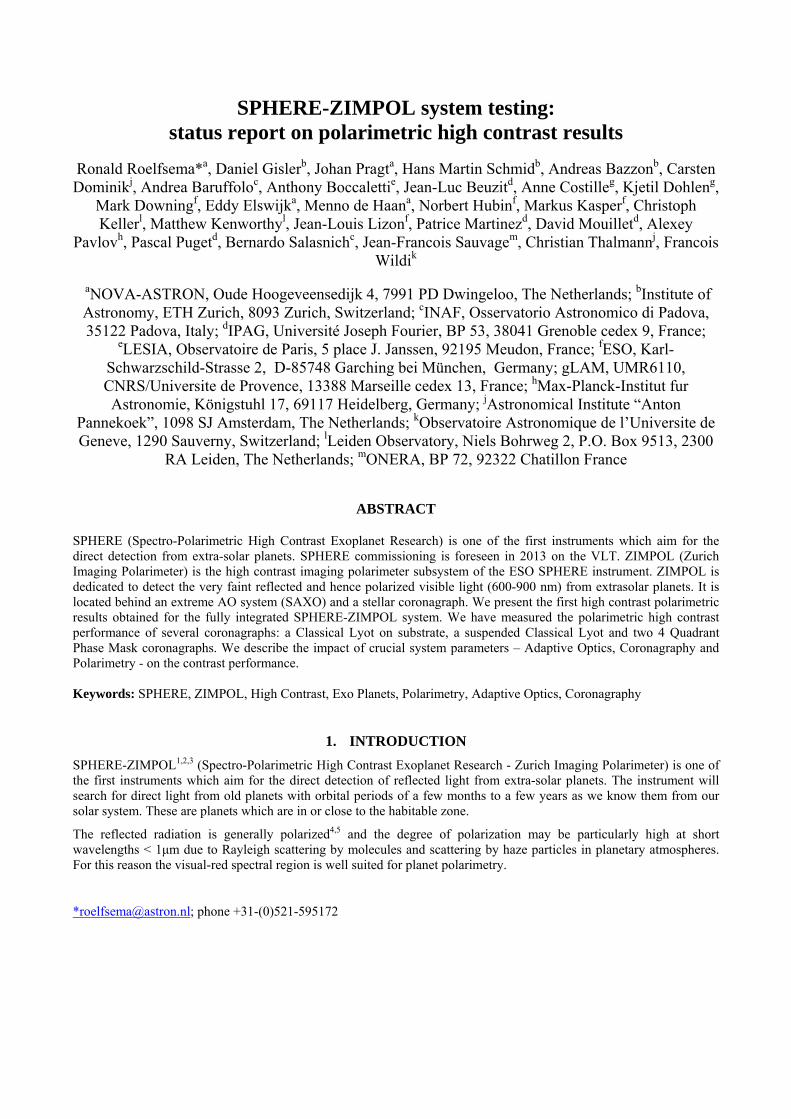
The basic functionality and the polarimetric behaviour of the coronagraphs under high Strehl non-turbulence conditions have been verified in the laboratory. The results are shown in Figure 3. Also shown are the results from an Apodized Phase Plate14 (APP). The APP will not be available on ZIMPOL during the first period of operation but is foreseen as a future upgrade. From the second row of images in Figure 3 we see that a polarimetric imprint is observed that is closely linked to the diffraction pattern from the coronagraphs. These patterns are not ‘real’ polarization signals that are caused by the coronagraphs themselves since we don’t observe the patterns if we reduce the Strehl ratio. However, the patterns are caused by small low order differential wave front errors introduced by the FLC polarization modulator. A switch of the

FLC modulator will cause a small differential tilt of the beam that will show up as a small differential shift in the image plane. In the polarization signal, i.e. the difference of the two images of each FLC state, the shift will leave a typical residual pattern as seen in Figure 3. Since this effect is expected to be a stable and constant in time a Double Difference measurement by means of the HWP2 switch will be used to mitigate this effect.

Figure 3 Coronagraphic intensity (top row) and polarization (bottom row) images at 820 nm (filter width 20 nm). Circles have radius 100 mas (4.7 λ/D at 820 nm).(1st column) 3λ/D on substrate (2nd column) 5λ/D suspended (3rd column) 4QPM2 (4th column) APP-mask. The images are recorded at a high Strehl test bench without induced turbulence.

ZIMPOL is equipped with several filter wheels: one common wheel and two non-common wheels in each arm. Among many other filters the common wheel contains several Neutral Density (ND) filters to control the flux levels. The ND-filters can be combined with the transmission filters in the non-common wheels. For our tests we have used the V (550/80) , NR (655/60), NI (820/80) and VBB (750/290) filters where the numbers in brackets express the filter Central Wavelength/BandWidth in nm.

2.4 Single Difference – ZIMPOL Polarimeter

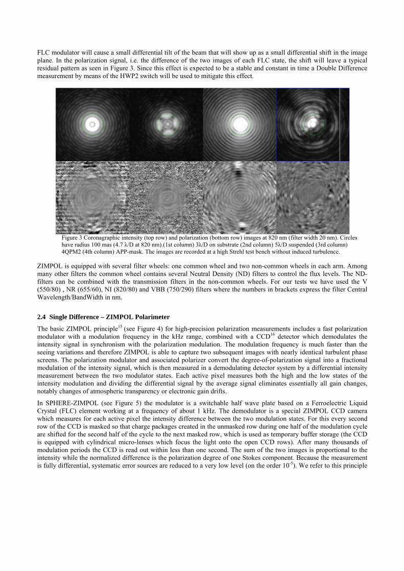
The basic ZIMPOL principle15 (see Figure 4) for high-precision polarization measurements includes a fast polarization modulator with a modulation frequency in the kHz range, combined with a CCD16 detector which demodulates the intensity signal in synchronism with the polarization modulation. The modulation frequency is much faster than the seeing variations and therefore ZIMPOL is able to capture two subsequent images with nearly identical turbulent phase screens. The polarization modulator and associated polarizer convert the degree-of-polarization signal into a fractional modulation of the intensity signal, which is then measured in a demodulating detector system by a differential intensity measurement between the two modulator states. Each active pixel measures both the high and the low states of the intensity modulation and dividing the differential signal by the average signal eliminates essentially all gain changes, notably changes of atmospheric transparency or electronic gain drifts.

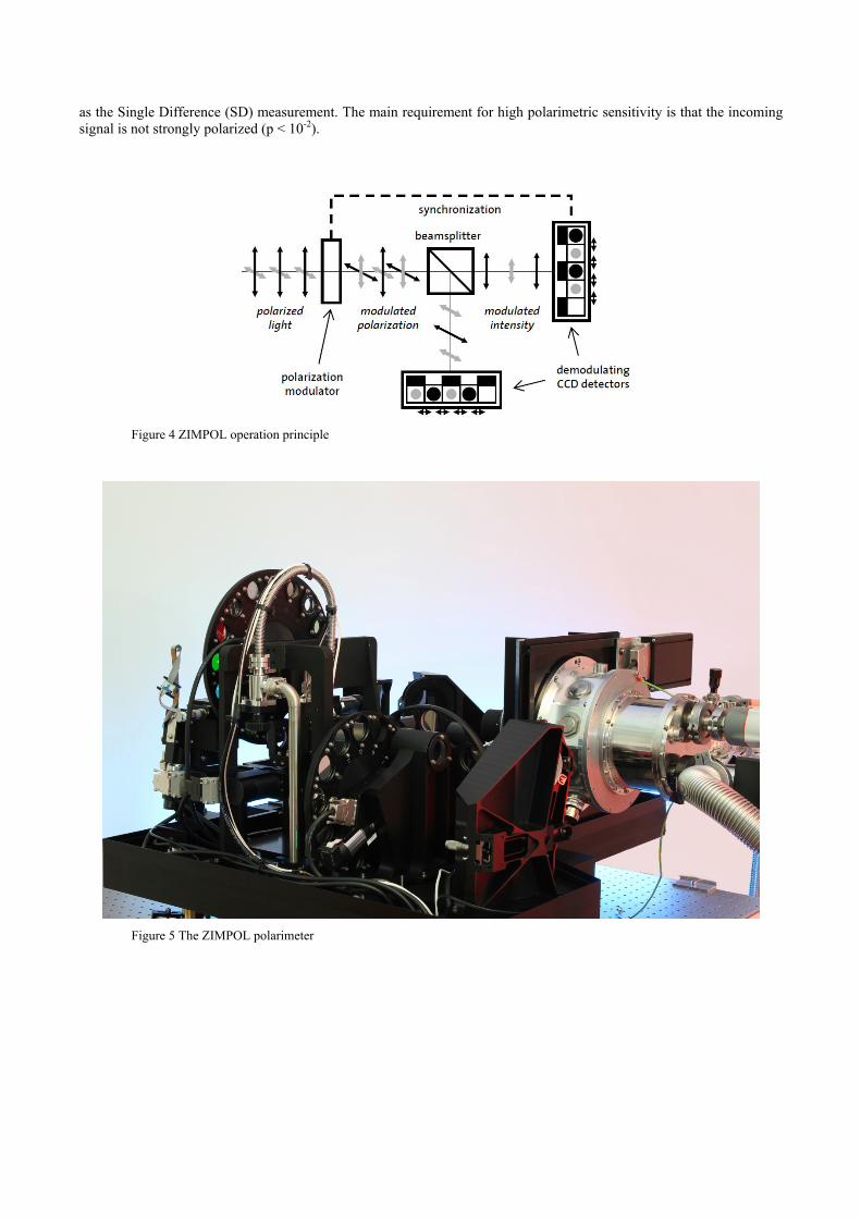
In SPHERE-ZIMPOL (see Figure 5) the modulator is a switchable half wave plate based on a Ferroelectric Liquid Crystal (FLC) element working at a frequency of about 1 kHz. The demodulator is a special ZIMPOL CCD camera which measures for each active pixel the intensity difference between the two modulation states. For this every second row of the CCD is masked so that charge packages created in the unmasked row during one half of the modulation cycle are shifted for the second half of the cycle to the next masked row, which is used as temporary buffer storage (the CCD is equipped with cylindrical micro-lenses which focus the light onto the open CCD rows). After many thousands of modulation periods the CCD is read out within less than one second. The sum of the two images is proportional to the intensity while the normalized difference is the polarization degree of one Stokes component. Because the measurement is fully differential, systematic error sources are reduced to a very low level (on the order 10-5). We refer to this principle

as the Single Difference (SD) measurement. The main requirement for high polarimetric sensitivity is that the incoming signal is not strongly polarized (p < 10-2).

Figure 4 ZIMPOL operation principle

Figure 5 The ZIMPOL polarimeter

2.5 Double Difference – HWP2 switch

By rotating a half-wave plate (HWP2) far upstream in the optical path by 45◦, the sign of the incoming Stokes Q polarization is reversed. The instrumental aberrations, on the other hand, remain unchanged, resulting in the same background landscape as before. If the polarization images before and after the signal switching are subtracted from one another, the real polarization signals of the astronomical target add up constructively while the static background is canceled out. This method is only effective down to the level at which the background can be reproduced in the second image; any change to the optical path on the time scale of the signal switching (i.e. temporal differential aberrations) will lead to residual structures surviving in the double-difference image and will limit the detection of faint signals. We refer to this principal as the Double Difference (DD) measurement.

The ultimate performance of astronomical high contrast instruments is limited by quasi-static speckles17. These are speckles that evolve relatively slowly in time on time scales in the order of several minutes. They are caused by small variations in wave front errors due to slow thermal drift of the instrument and telescope tracking that are not seen by the wave front sensor. To calibrate this effect HWP2 is foreseen to be switched about every 5 minutes during observation.

To summarize the key importance of the HWP2 switch:

- Reverse the sign of the planet polarization

- Calibrate the FLC differential Wave Front Error

- Provide a temporal switch to calibrate the quasi static speckle

2.6 Turbulence Simulator

A turbulence simulator (TSIM) is located at the optical entrance of the SPHERE bench. The turbulence is generated by a rotating phase screen18. For our tests we have used typical conditions of 0.85 asec seeing and 10 m/s windspeed. This is very close to the ‘normal’ conditions that are foreseen at the VLT (0.85 asec and 12.5 m/s windspeed). The turbulence simulator is fed by a high energetic broad band source (Energetiq LDLS EQ-99FLC). This source produces a reasonable flat spectrum over the 500 – 790 nm band and has peaks at 820 and 880 nm.

2.7 Instrument Polarization

To achieve high contrast performance the polarized input signal at the ZIMPOL detectors must be lower than about 1%. Therefore we have characterized the polarimetric behaviour of the turbulence simulator and the SPHERE optical bench19. The polarization Q/I measured at the ZIMPOL detectors is a combination of polarization introduced before HWP2 (the Turbulence Simulator and mirror M4) and polarization introduced after HWP2 (the SPHERE optical components – in particular the derotator). The HWP2 switch allows disentangling these two contributions. As expected the TSIM Q/I polarization oscillates with the HWP2 rotation whereas the SPERE polarization is essentially independent of the HWP2 rotation (see Figure 6). Also we observe a strong dependence on wavelength. To minimize the input polarization at the ZIMPOL detectors we have used a twofold strategy

1. To minimize the TSIM input polarization the HWP2 rotation is set at a Q/I zero crossing as can be found from Figure 6 for each filter. The subsequent 45 degree HWP2 switch will also be at a zero crossing

2. To minimize the SPHERE input polarization we have used the ZIMPOL internal Polarization Compensator20.

Figure 6 Instrument polarization as function of HWP2 rotation angle introduced before (TSIM & M4) and after (SPHERE) HWP2 for detector Callas.

3. DATA REDUCTION

This section describes how we reduce the high contrast data and how we estimate the contrast ratios from the reduced frames. It should be noted that we don’t use a weak polarized point source to simulate a planet in our setup. The contrast is estimated from the noise level in the final averaged images. We will present our results as plots of azimuthal statistics as function of radial separation from the PSF peak. We use as notation conventions a single overbar for the azimuthal average and a double overbar for the azimuthal standard deviation. The azimuthal statistics are calculated over a ring with the width of a resolution element λ/D, i.e. 3 pixels. The basic data reduction steps are as follows. Bias is subtracted based on the pre –and overscan regions of the individual frames. The data is split in two datasets corresponding to the two HWP2 settings of the DD measurement. Each dataset is split up in sets of two consecutive frames and these sets are converted to Stokes Q taken into account the ZIMPOL CCD double phase mode operation. The Q frames are averaged and the end results are two final frames where each frame corresponds to a SD measurement. The two averaged SD frames are subtracted and divided by two to yield the final DD Stokes Q frame. An identical procedure is applied where the sets of two consecutive frames are converted to Stokes I taken into account the ZIMPOL double phase mode operation. This will yield the final DD Stokes I frame. From these two final DD frames it’s obvious to obtain the overall normalized Stokes Q/I frame. We will now derive a simple expression for the polarimetric contrast that we will use to further process the reduced data. The strength Δp of the polarized planet signal in the unpolarized star halo is given by

int

Q p Fp

I H

(1)

Here p is the planet polarization and F is planet flux level. intH is the azimuthal average of the final DD Stokes I frame. We are interested in how much stronger the planet signal Δp is than the background noise level. Therefore we define the statistical significance level σ of the detection as

pol

p

H (2)

Here polH is the polarization background noise level that is estimated from the azimuthal standard deviation of the final

DD Stokes Q/I frame. The polarimetric contrast level Cp is given by the ratio of the polarized flux level p×F in the planet PSF and the peak flux level Speak of the central star PSF:

int

polp ppeak peak

p F HC C H

S S

(3)

From this expression we arrive at the intuitive conclusion that the contrast is proportional to the product of the normalized coronagraph intensity pattern and the polarimetric noise level. We will use a significance level σ = 5 for a successful planet detection. In section Error! Reference source not found. we derive an expression for the polarimetric contrast of a Jupiter size polarized planet. This will allow a direct comparison of the instrument performance and the planet detection probability. To calculate the contrast we need an experimental estimate of the strength Speak of a reference PSF. We estimate this value by taken a non-coronagraphic PSF with the Turbulence Simulator and measure the total flux FREF in this image. We also construct an ideal model Airy pattern with a peak value equal to one and we also measure the total flux FAIRY in the Airy pattern. As reference image we take an Airy pattern with total flux equal to FREF. Therefore we estimate the peak level of the reference as Speak = (FREF/FAIRY). We will use this value as normalization factor for all presented azimuthal average curves. The photon noise level can be obtained from experimental data as

_

int

1 1phot noise

phot

HN gain N H

(4)

where Nphot is the total number of photons acquired during the exposure, gain is the CCD gain (10.5 e/ADU) and N is the total number of acquired frames. As last point we will define the ultimate contrast that can be reached during a high contrast measurement. This limit is set by the Photon Noise and we will define it similar to equation (3) as

int

_phot noiseultimatepeak

HC H

S

(5)

4. PERFORMANCE MODELING

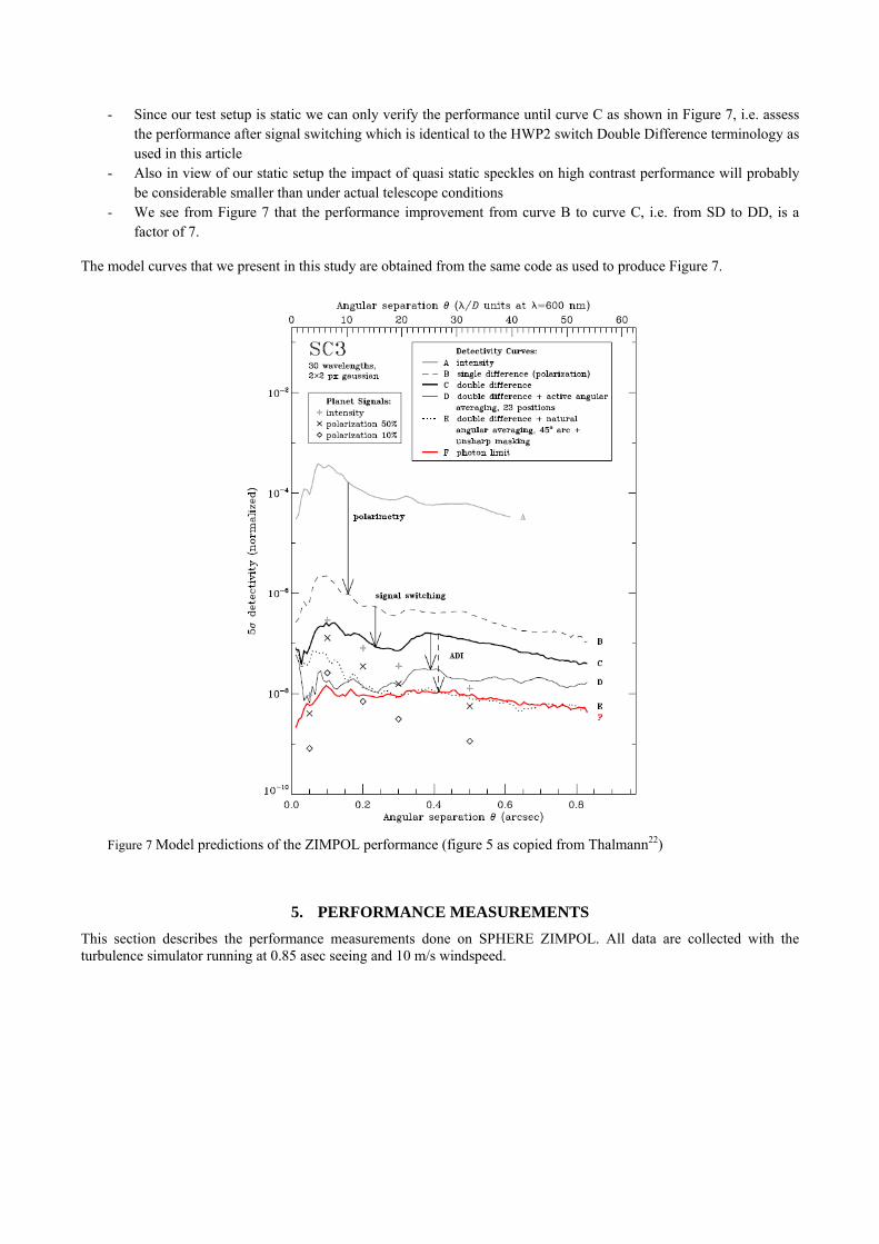
The ZIMPOL performance simulations are done with the CAOS21 problem solving environment and are extensively described in Thalmann22. We copy the main performance predictions from Thalmann and display them in Figure 7. In the context of the performance verification as described in this article we make the following remarks:

- Since our test setup is static we can only verify the performance until curve C as shown in Figure 7, i.e. assess the performance after signal switching which is identical to the HWP2 switch Double Difference terminology as used in this article

- Also in view of our static setup the impact of quasi static speckles on high contrast performance will probably be considerable smaller than under actual telescope conditions

- We see from Figure 7 that the performance improvement from curve B to curve C, i.e. from SD to DD, is a factor of 7.

The model curves that we present in this study are obtained from the same code as used to produce Figure 7.

Figure 7 Model predictions of the ZIMPOL performance (figure 5 as copied from Thalmann22)

5. PERFORMANCE MEASUREMENTS

This section describes the performance measurements done on SPHERE ZIMPOL. All data are collected with the turbulence simulator running at 0.85 asec seeing and 10 m/s windspeed.

5.1 Adaptive Optics

Non-coronagraphic point source intensity images under atmospheric turbulent conditions are obtained in the V, NR, NI and VBB filters. The results for each filter are shown in Figure 8. From the figure we obviously observe the scaling of the diameter of the AO control radius at 20 λ/D with wavelength and the speckle elongation for the broad band VBB filter. The azimthal averages of the measured and modeled profiles are shown in Figure 9. We conclude a good match between measurements and model from this figure. Table 2 lists the FWHM and Strehl for each filter with obvious performance improvement for increasing wavelength.

Figure 8 Non-coronagraphic point source intensity images under atmospheric turbulent conditions (0.85 asec seeing and 10 m/s windspeed) for filters NR, NI and VBB (left to right). The AO control radius is at 20 λ/D.

Table 2 AO performance under atmospheric turbulent conditions (0.85 asec seeing and 10 m/s windspeed) for several filters 

Filter FWHM (mas) Airy pattern (calculated)

FWHM (mas) (measured)

Strehl (measured)

NR 19.2 21.1 0.46 NI 24.0 24.9 0.63

VBB 22.0 27.0 0.52

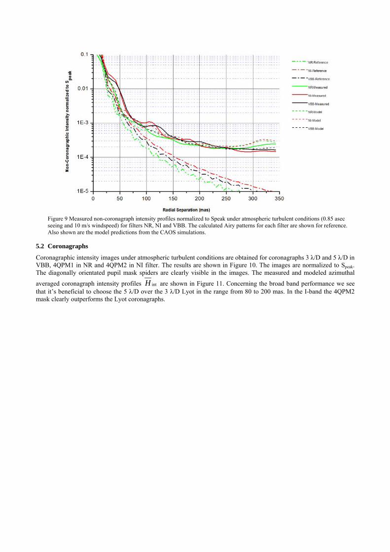
Figure 9 Measured non-coronagraph intensity profiles normalized to Speak under atmospheric turbulent conditions (0.85 asec seeing and 10 m/s windspeed) for filters NR, NI and VBB. The calculated Airy patterns for each filter are shown for reference. Also shown are the model predictions from the CAOS simulations.

5.2 Coronagraphs

Coronagraphic intensity images under atmospheric turbulent conditions are obtained for coronagraphs 3 λ/D and 5 λ/D in VBB, 4QPM1 in NR and 4QPM2 in NI filter. The results are shown in Figure 10. The images are normalized to Speak. The diagonally orientated pupil mask spiders are clearly visible in the images. The measured and modeled azimuthal

averaged coronagraph intensity profiles intH are shown in Figure 11. Concerning the broad band performance we see that it’s beneficial to choose the 5 λ/D over the 3 λ/D Lyot in the range from 80 to 200 mas. In the I-band the 4QPM2 mask clearly outperforms the Lyot coronagraphs.

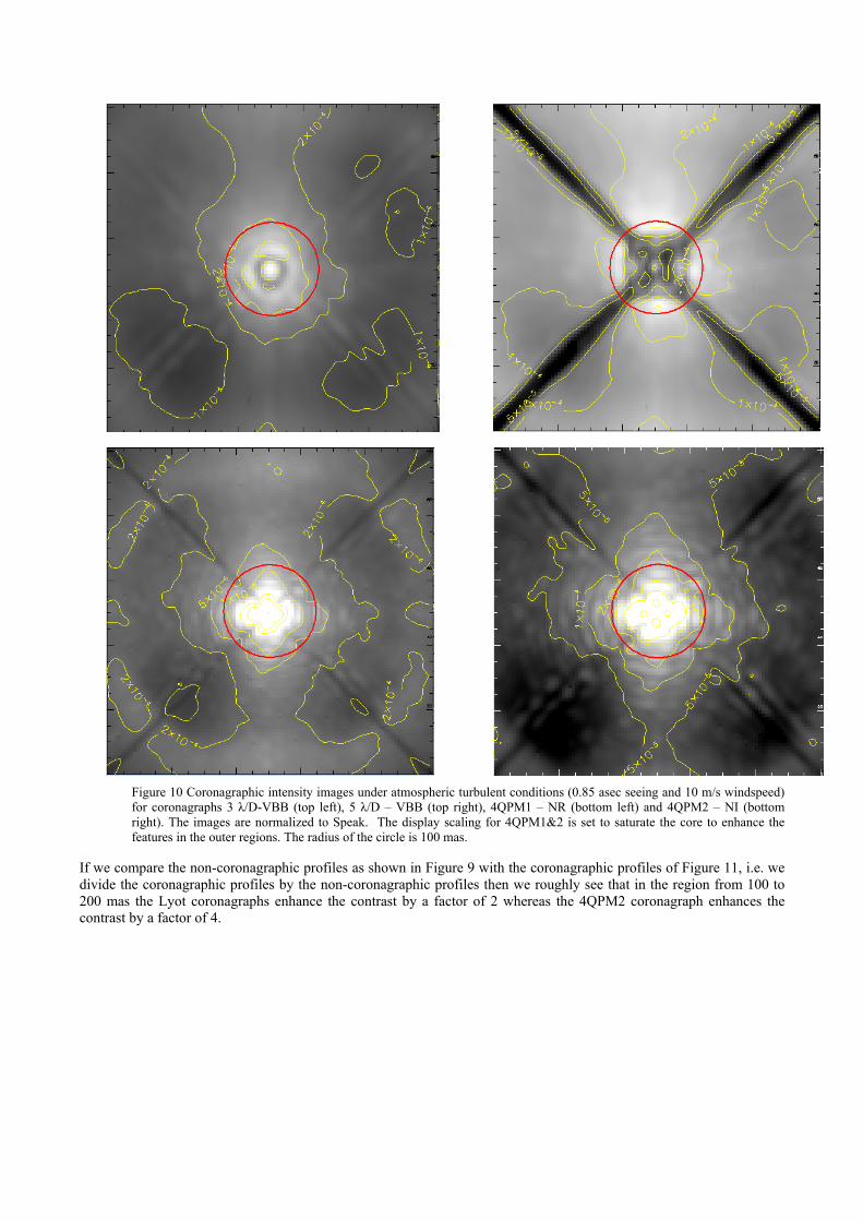
Figure 10 Coronagraphic intensity images under atmospheric turbulent conditions (0.85 asec seeing and 10 m/s windspeed) for coronagraphs 3 λ/D-VBB (top left), 5 λ/D – VBB (top right), 4QPM1 – NR (bottom left) and 4QPM2 – NI (bottom right). The images are normalized to Speak. The display scaling for 4QPM1&2 is set to saturate the core to enhance the features in the outer regions. The radius of the circle is 100 mas.

If we compare the non-coronagraphic profiles as shown in Figure 9 with the coronagraphic profiles of Figure 11, i.e. we divide the coronagraphic profiles by the non-coronagraphic profiles then we roughly see that in the region from 100 to 200 mas the Lyot coronagraphs enhance the contrast by a factor of 2 whereas the 4QPM2 coronagraph enhances the contrast by a factor of 4.

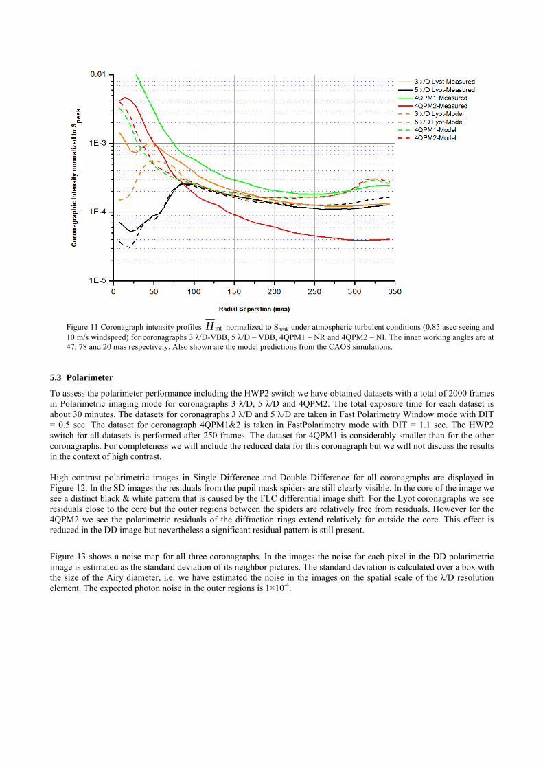
Figure 11 Coronagraph intensity profiles intH normalized to Speak under atmospheric turbulent conditions (0.85 asec seeing and 10 m/s windspeed) for coronagraphs 3 λ/D-VBB, 5 λ/D – VBB, 4QPM1 – NR and 4QPM2 – NI. The inner working angles are at 47, 78 and 20 mas respectively. Also shown are the model predictions from the CAOS simulations.

5.3 Polarimeter

To assess the polarimeter performance including the HWP2 switch we have obtained datasets with a total of 2000 frames in Polarimetric imaging mode for coronagraphs 3 λ/D, 5 λ/D and 4QPM2. The total exposure time for each dataset is about 30 minutes. The datasets for coronagraphs 3 λ/D and 5 λ/D are taken in Fast Polarimetry Window mode with DIT = 0.5 sec. The dataset for coronagraph 4QPM1&2 is taken in FastPolarimetry mode with DIT = 1.1 sec. The HWP2 switch for all datasets is performed after 250 frames. The dataset for 4QPM1 is considerably smaller than for the other coronagraphs. For completeness we will include the reduced data for this coronagraph but we will not discuss the results in the context of high contrast. High contrast polarimetric images in Single Difference and Double Difference for all coronagraphs are displayed in Figure 12. In the SD images the residuals from the pupil mask spiders are still clearly visible. In the core of the image we see a distinct black & white pattern that is caused by the FLC differential image shift. For the Lyot coronagraphs we see residuals close to the core but the outer regions between the spiders are relatively free from residuals. However for the 4QPM2 we see the polarimetric residuals of the diffraction rings extend relatively far outside the core. This effect is reduced in the DD image but nevertheless a significant residual pattern is still present.

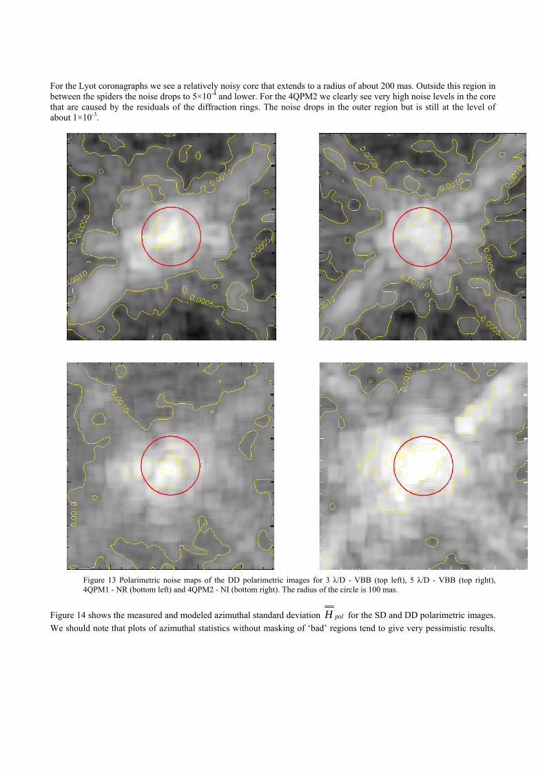
Figure 13 shows a noise map for all three coronagraphs. In the images the noise for each pixel in the DD polarimetric image is estimated as the standard deviation of its neighbor pictures. The standard deviation is calculated over a box with the size of the Airy diameter, i.e. we have estimated the noise in the images on the spatial scale of the λ/D resolution element. The expected photon noise in the outer regions is 1×10-4.

Figure 12 High contrast polarimetric images in Single Difference (left) and Double Difference (right) for coronagraphs 3 λ/D - VBB, 5 λ/D - VBB, 4QPM1 - NR and 4QPM2 - NI (from top to bottom). All images are scaled symmetrical around the average value of the image. However, the cut levels of the scaling of the DD images are set to a quarter of the cut levels of the SD images to enhance the features in the outer regions of the DD images. The radius of the circle is 100 mas.

For the Lyot coronagraphs we see a relatively noisy core that extends to a radius of about 200 mas. Outside this region in between the spiders the noise drops to 5×10-4 and lower. For the 4QPM2 we clearly see very high noise levels in the core that are caused by the residuals of the diffraction rings. The noise drops in the outer region but is still at the level of about 1×10-3.

Figure 13 Polarimetric noise maps of the DD polarimetric images for 3 λ/D - VBB (top left), 5 λ/D - VBB (top right), 4QPM1 - NR (bottom left) and 4QPM2 - NI (bottom right). The radius of the circle is 100 mas.

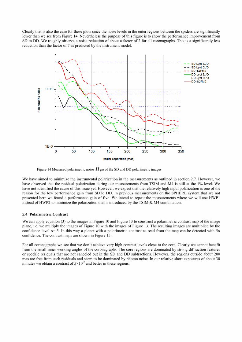
Figure 14 shows the measured and modeled azimuthal standard deviation polH for the SD and DD polarimetric images.

We should note that plots of azimuthal statistics without masking of ‘bad’ regions tend to give very pessimistic results.

Clearly that is also the case for these plots since the noise levels in the outer regions between the spiders are significantly lower than we see from Figure 14. Nevertheless the purpose of this figure is to show the performance improvement from SD to DD. We roughly observe a noise reduction of about a factor of 2 for all coronagraphs. This is a significantly less reduction than the factor of 7 as predicted by the instrument model.

Figure 14 Measured polarimetric noise polH of the SD and DD polarimetric images

We have aimed to minimize the instrumental polarization in the measurements as outlined in section 2.7. However, we have observed that the residual polarization during our measurements from TSIM and M4 is still at the 1% level. We have not identified the cause of this issue yet. However, we expect that the relatively high input polarization is one of the reason for the low performance gain from SD to DD. In previous measurements on the SPHERE system that are not presented here we found a performance gain of five. We intend to repeat the measurements where we will use HWP1 instead of HWP2 to minimize the polarization that is introduced by the TSIM & M4 combination.

5.4 Polarimetric Contrast

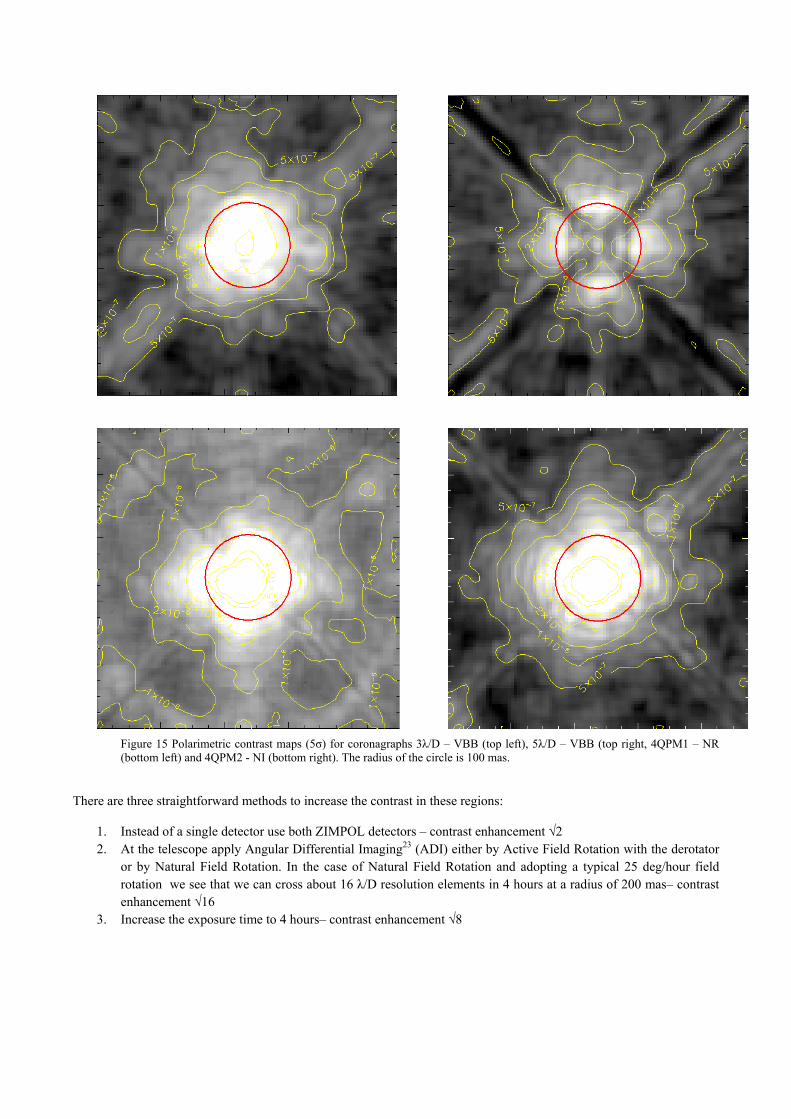
We can apply equation (3) to the images in Figure 10 and Figure 13 to construct a polarimetric contrast map of the image plane, i.e. we multiply the images of Figure 10 with the images of Figure 13. The resulting images are multiplied by the confidence level σ= 5. In this way a planet with a polarimetric contrast as read from the map can be detected with 5σ confidence. The contrast maps are shown in Figure 15. For all coronagraphs we see that we don’t achieve very high contrast levels close to the core. Clearly we cannot benefit from the small inner working angles of the coronagraphs. The core regions are dominated by strong diffraction features or speckle residuals that are not canceled out in the SD and DD subtractions. However, the regions outside about 200 mas are free from such residuals and seem to be dominated by photon noise. In our relative short exposures of about 30 minutes we obtain a contrast of 5×10-7 and better in these regions.

Figure 15 Polarimetric contrast maps (5σ) for coronagraphs 3λ/D – VBB (top left), 5λ/D – VBB (top right, 4QPM1 – NR (bottom left) and 4QPM2 - NI (bottom right). The radius of the circle is 100 mas.

There are three straightforward methods to increase the contrast in these regions:

1. Instead of a single detector use both ZIMPOL detectors – contrast enhancement √2 2. At the telescope apply Angular Differential Imaging23 (ADI) either by Active Field Rotation with the derotator

or by Natural Field Rotation. In the case of Natural Field Rotation and adopting a typical 25 deg/hour field rotation we see that we can cross about 16 λ/D resolution elements in 4 hours at a radius of 200 mas– contrast enhancement √16

3. Increase the exposure time to 4 hours– contrast enhancement √8

This should give as a total contrast enhancement of a factor 16 and therefore we conclude that we can achieve a 5σ polarimetric contrast of 3 × 10-8 at an angular separation of 200 mas in an exposure time of 4 hours.

6. CONCLUSIONS

We have done first system level testing to assess the high contrast performance of SPHERE-ZIMPOL. We have taken relatively short exposures of about 30 minutes each to verify the performance of four coronagraphs: the 3 λ/D and 5 λ/D Lyot coronagraphs in VBB filter and the 4QPM1 & 2 coronagraphs in NR and NI filter respectively. We observe excellent AO and coronagraph performance in agreement with the model predictions. However, in general we observe relatively high polarization noise levels close to the PSF core where residuals are not sufficiently removed by either SD or DD subtraction. The measured SD to DD performance improvement is only a factor 2 contrary to the model predictions of a factor 7. We suspects that the relatively high polarization levels of about 1% are part of the cause of this discrepancy. Beyond a radius of 200 mas and in between the pupil/image mask spiders we enter the photon noise limited regime. In this region we estimate that we can achieve a 5σ polarimetric contrast of 3 × 10-8 at an angular separation of 200 mas in an exposure time of 4 hours. At the time that our measurements were performed the SPHERE system was not optimized for visible high contrast performance testing yet. We will perform final high contrast measurements in September 2013 where we expect the following improvements:

- NCPA correction - Coronagraph automatic fine centering template - Reduction of polarization levels to < 0.1% by using HWP1 to minimize the TSIM & M4 induced polarization - Longer exposure times

In a parallel trajectory we will conduct laboratory measurements to investigate the origin of the relatively large polarimetric residuals in the stellar PSF halo due to residual speckles and diffraction features. In addition we will apply more advanced data processing techniques to increase the contrast.

REFERENCES

[1] Schmid, H. M., Beuzit, J.-L., Feldt, M., Gisler, D., Gratton, R., Henning, T., Joos, F., Kasper, M., Lenzen, R., Mouillet, D., Moutou, C., Quirrenbach, A., Stam, D. M., Thalmann, C., Tinbergen, J., Verinaud, C., Waters, R., and Wolstencroft, R., “Search and investigation of extra-solar planets with polarimetry,” IAU Colloq. 200, 165–170 (2006)

[2] D. Gisler, H.M. Schmid, C. Thalmann, H.P. Povel, J.O. Stenflo, F. Joos, M. Feldt, R. Lenzen, J. Tinbergen, R. Gratton, R. Stuik, D.M. Stam, W. Brandner, S. Hippler, M. Turatto, R. Neuhäuser, C. Dominik, A. Hatzes, Th. Henning, J. Lima, A. Quirrenbach, L.B.F.M. Waters, G. Wuchterl, H. Zinnecker, “CHEOPS/ZIMPOL: a VLT instrument study for the polarimetric search of scattered light from extrasolar planets,” Proc. SPIE 5492, 463-474 (2004)

[3] Beuzit, J.-L., Feldt, M., Dohlen, K., Mouillet, D., Puget, P., Antichi, J., Baruffolo, A., Baudoz, P., Berton, A., Boccaletti, A., Carbillet, M., Charton, J., Claudi, R., Downing, M., Feautrier, P., Fedrigo, E., Fusco, T., Gratton, R., Hubin, N., Kasper, M., Langlois, M., Moutou, C., Mugnier, L., Pragt, J., Rabou, P., Saisse, M., Schmid, H. M., Stadler, E., Turrato, M., Udry, S., Waters, R., and Wildi, F., “SPHERE: A ‘Planet Finder’ Instrument for the VLT,” The Messenger 125, 29–34 (2006)

[4] D. M. Stam, “Spectropolarimetric signatures of Earth-like extrasolar planets,” A&A 482, 989-1007 (2008) [5] E. Buenzli, H.M. Schmid, “A grid of polarization models for Rayleigh scattering planetary atmospheres,”

Astron. Astrophys. 504, 259-276, 2009 [6] Julien Milli, David Mouillet, Dimitri Mawet, Hans Martin Schmid, Andreas Bazzon, Julien H. Girard, Kjetil

Dohlen, Ronald Roelfsema, “Prospects of detecting the polarimetric signature of the Earth-mass planet alpha Centauri B b with SPHERE / ZIMPOL,” A&A, (2013)

[7] Sascha P. Quanz, Hans Martin Schmid, Kerstin Geissler, Michael R. Meyer, Thomas Henning, Wolfgang Brandner, Sebastian Wolf, “VLT/NACO Polarimetric Differential Imaging of HD100546 - Disk Structure and Dust Grain Properties between 10-140 AU,” ApJ, 738 Issue 1, 23 (2011)

[8] Michihiro Takami et al, “High-Contrast Near-Infrared Imaging Polarimetry of the Protoplanetary Disk around RY Tau,” ApJ 772, Issue 2, 145 (2013)

[9] Kjetil Dohlen , Michel Saisse et al, “Manufacturing and integration of the IRDIS dual imaging camera and spectrograph for SPHERE,” Proc. SPIE 7735, (2010)

[10] Ricardo Claudi, “SPHERE IFS: The spectro differential imager of the VLT for exoplanets search,” Proc. SPIE 7735, (2010)

[11] Franco Joos, Esther Buenzli, Hans Martin Schmid and Christian Thalmann, “Reduction of polarimetric data using Mueller calculus applied to Nasmyth instruments,“ Proc. SPIE 7016, (2008)

[12] C. Petit , J.-F. Sauvage , A. Sevin ; A. Costille , T. Fusco , P. Baudoz , J.-L. Beuzit , T. Buey , J. Charton , K. Dohlen , P. Feautrier , E. Fedrigo , J.-L. Gach , N. Hubin , E. Hugot , M. Kasper , D. Mouillet , D. Perret , P. Puget , J.-C. Sinquin , C. Soenke , M. Suarez , F. Wildi, “The SPHERE XAO system SAXO: integration, test, and laboratory performance,” Proc. SPIE 8447, (2012)

[13] Rouan, D., Riaud, P., Boccaletti, A., Cl´enet, Y., and Labeyrie, A., “The Four-Quadrant Phase-MaskCoronagraph. I. Principle,” The Publications of the Astronomical Society of the Pacific 112, 1479–1486 (2000)

[14] Quanz, Sascha P.; Meyer, Michael R.; Kenworthy, Matthew A.; Girard, Julien H. V.; Kasper, Markus; Lagrange, Anne-Marie; Apai, Daniel; Boccaletti, Anthony; Bonnefoy, Mickaël; Chauvin, Gael; Hinz, Philip M.; Lenzen, Rainer, “First Results from Very Large Telescope NACO Apodizing Phase Plate: 4 μm Images of The Exoplanet β Pictoris b,” ApJ 722, 49 (2010)

[15] Povel, H. P., Aebersold, F., and Stenflo, J., “Charge-coupled device image sensor as a demodulator in a 2-D polarimeter with a piezoelastic modulator,” Appl. Opt. 29, 1186 (1990)

[16] Schmid, Hans-Martin; Downing, Mark; Roelfsema, Ronald; Bazzon, Andreas; Gisler, Daniel; Pragt, Johan; Cumani, Claudio; Salasnich, Bernardo; Pavlov, Alexey; Baruffolo, Andrea; Beuzit, Jean-Luc; Costille, Anne; Deiries, Sebastian; Dohlen, Kjetil; Dominik, Carsten; Elswijk, Eddy; Feldt, Markus; Kasper, Markus; Mouillet, David; Thalmann, Christian; Wildi, François, “Tests of the demodulating CCDs for the SPHERE / ZIMPOL imaging polarimeter,” Proc. SPIE 8446, (2012)

[17] P. Martinez, C. Loose, E. Aller Carpentier and M. Kasper, “Speckle temporal stability in XAO coronagraphic images,” A&A 541, A136 (2012)

[18] L. Jolissaint, “Optical Turbulence Generators for Testing Astronomical Adaptive Optics Systems: A Review and Designer Guide,” PASP 118, 1205-1224, (2006)

[19] Andreas Bazzon , Daniel Gisler , Ronald Roelfsema , Hans M. Schmid , Johan Pragt , Eddy Elswijk , Menno de Haan , Mark Downing , Bernardo Salasnich , Alexey Pavlov , Jean-Luc Beuzit , Kjetil Dohlen ,David Mouillet , François Wildi, “SPHERE / ZIMPOL: characterization of the FLC polarization modulator,” Proc. SPIE 8446, (2012)

[20] Ronald Roelfsema , Daniel Gisler , Johan Pragt , Hans Martin Schmid , Andreas Bazzon , Carsten Dominik , Andrea Baruffolo , Jean-Luc Beuzit , Julien Charton , Kjetil Dohlen , Mark Downing , Eddy Elswijk , Markus Feldt , Menno de Haan , Norbert Hubin , Markus Kasper , Christoph Keller , Jean-Louis Lizon , David Mouillet , Alexey Pavlov , Pascal Puget , Sylvain Rochat , Bernardo Salasnich , Peter Steiner , Christian Thalmann , Rens Waters , François Wildi, “The ZIMPOL high contrast imaging polarimeter for SPHERE: sub-system test results,” Proc. SPIE 8151, (2011)

[21] Carbillet, M., Boccaletti, A., Thalmann, C., Fusco, T., Vigan, A., Mouillet, D., and Dohlen, K., “The software package SPHERE: a numerical tool for end-to-end simulations of the VLT instrument SPHERE,” Proc. Spie 7015, (2008)

[22] Thalmann, Christian, Schmid, Hans M., Boccaletti, Anthony, Mouillet, David, Dohlen, Kjetil, Roelfsema, Ronald, Carbillet, Marcel, Gisler, Daniel, Beuzit, Jean-Luc, Feldt, Markus, Gratton, Raffaele, Joos, Franco, Keller, Christoph U., Kragt, Jan, Pragt, Johan H., Puget, Pascal, Rigal, Florence, Snik, Frans, Waters, Rens, Wildi, François, “SPHERE ZIMPOL: overview and performance simulation,” Proc. SPIE 7014, 70143F, (2008)

[23] Marois, C., Lafreni`ere, D., Doyon, R., Macintosh, B., and Nadeau, D., “Angular Differential Imaging: A Powerful High-Contrast Imaging Technique,” The Astrophysical Journal 641, 556–564 (2006)