Spin-orbit coupling in curved graphene, fullerenes, nanotubes, and nanotube caps
Daniel Huertas-Hernando,1 F. Guinea,2 and Arne Brataas1,3
1Department of Physics, Norwegian University of Science and Technology, N-7491, Trondheim, Norway2Instituto de Ciencia de Materiales de Madrid, CSIC, Cantoblanco E28049 Madrid, Spain
3Centre for Advanced Study, Drammensveien 78, 0271 Oslo, Norway�Received 23 June 2006; revised manuscript received 16 August 2006; published 24 October 2006�
A continuum model for the effective spin-orbit interaction in graphene is derived from a tight-binding modelwhich includes the � and � bands. We analyze the combined effects of the intra-atomic spin-orbit coupling,curvature, and applied electric field, using perturbation theory. We recover the effective spin-orbit Hamiltonianderived recently from group theoretical arguments by Kane and Mele. We find, for flat graphene, that theintrinsic spin-orbit coupling �int��2 and the Rashba coupling due to a perpendicular electric field E, �E��,where � is the intra-atomic spin-orbit coupling constant for carbon. Moreover we show that local curvature ofthe graphene sheet induces an extra spin-orbit coupling term �curv��. For the values of E and curvature profilereported in actual samples of graphene, we find that �int��E��curv. The effect of spin-orbit coupling onderived materials of graphenelike fullerenes, nanotubes, and nanotube caps, is also studied. For fullerenes, only�int is important. Both for nanotubes and nanotube caps �curv is in the order of a few Kelvins. We reproducethe known appearance of a gap and spin-splitting in the energy spectrum of nanotubes due to the spin-orbitcoupling. For nanotube caps, spin-orbit coupling causes spin-splitting of the localized states at the cap, whichcould allow spin-dependent field-effect emission.
A single layer of carbon atoms in a honeycomb lattice,graphene, is an interesting two-dimensional system due to itsremarkable low energy electronic properties,1–3 e.g., a zerodensity of states at the Fermi level without an energy gap,and a linear, rather than parabolic, energy dispersion aroundthe Fermi level. The electronic properties of the many real-izations of the honeycomb lattice of carbon such, e.g., bulkgraphite �three dimensional �3D��, carbon nanotube wires�one dimensional �1D��, carbon nanotube quantum dots �zerodimensional �0D��, and curved surfaces such as fullerenes,have been studied extensively during the last decade. How-ever, its two-dimensional �2D� version, graphene, a stableatomic layer of carbon atoms, remained for long ellusiveamong the known crystalline structures of carbon. Only re-cently, the experimental realization of stable, highly crystal-line, single layer samples of graphene,4–7 have been possible.Such experimental developments have generated a renewedinterest in the field of two-dimensional mesoscopic systems.The peculiar electronic properties of graphene are quite dif-ferent from that of 2D semiconducting heterostructuressamples. It has been found that the integer Hall effect ingraphene is different than the “usual” quantum Hall effect insemiconducting structures.8–11 Moreover, it has been theo-retically suggested that a variety of properties, e.g., weak�anti�localization,12–17 shot-noise18 and anomalous tunneling,Klein’s paradox,19 are qualitatively different from the behav-ior found in other 2D systems during the last decades. Allthese predictions can now be directly investigated by experi-ments. The activity in graphene, both theoretically and ex-perimentally, is at present very intense. However so far, thework has mainly focused on �i� the fact that the unit cell isdescribed by two inequivalent triangular sublattices A and Bintercalated, and �ii� there are two independent k points, K
and K�, corresponding to the two inequivalent corners of theBrillouin zone of graphene. The Fermi level is located atthese K and K� points and crosses the � bands of graphene�see Fig. 1 for details�. These two features provide an exoticfourfold degeneracy of the low energy �spin-degenerate�states of graphene. These states can be described by two setsof two-dimensional chiral spinors which follow the masslessDirac-Weyl equation and describe the electronic states of thesystem near the K and K� points where the Fermi level islocated. Neutral graphene has one electron per carbon atomin the � band, so the band below the Fermi level is full�electronlike states� and the band above it is empty �holelikestates�. Electrons and holes in graphene behave like relativ-istic Dirac fermions. The Fermi level can be moved by agate voltage underneath the graphene sample.4 State-of-the-art samples are very clean, with mobilities ��15 000 cm2 V−1 s−1,6 so charge transport can be ballisticfor long distances across the sample. From the mobilities ofthe actual samples, it is believed that impurity scattering isweak. Furthermore, it has been recently suggested that thechiral nature of graphene carriers makes disordered regionstransparent for these carriers independently of the disorder,as long as it is smooth on the scale of the latticeconstant.13,14,20
Less attention has been given to the spin so far. The maininteractions that could affect the spin degree of freedom ingraphene seem to be the spin-orbit coupling and exchangeinteraction. It is not known to which extent magnetic impu-rities are present in actual graphene samples. Their effectseems small though, as noticed recently when investigatingweak localization and universal conductance fluctuations ingraphene.14 Spin-orbit interaction in graphene is supposed tobe weak, due to the low atomic number Z=6 of carbon.Therefore both spin-splitting and spin-flip due to the combi-nation of spin-orbit and scattering due to disorder is sup-posed to be not very important. As a result, the spin degree
of freedom is assumed to have a minor importance and spindegenerate states are assumed. Besides, the spin degeneracyis considered to be “trivial” in comparison to the fourfolddegeneracy previously mentioned, described by a pseudospindegree of freedom. At present, there is a large activity in thestudy of the dynamics of this pseudospin degree offreedom.8–26
We think that the physics of the electronic spin ingraphene must be investigated in some detail, however. Al-though it could be that the electronic spin is not as importantor exotic as the pseudospin when studying bulk properties,edge states may be quite different. Induced magnetism at theedges of the surface of graphite samples irradiated with pro-tons have been reported.27 Moreover, perspectives of spin-tronic applications in graphene could be very promising, so itis important to clarify the role of the electronic spin. This isone of the main purposes of the present paper. Moreover, wefeel that the existent knowledge about the spin-orbit interac-tion in graphene is not yet complete24 and that certain, bothquantitative and qualitative, points must be discussed inmore detail. That is why we focus our discussion on the
spin-orbit coupling. The effect of other interactions as theexchange interaction will be discussed elsewhere.
Spin-orbit coupling in graphene has an intrinsic part,completely determined from the symmetry properties of thehoneycomb lattice. This is similar to the Dresselhauss spin-orbit interaction in semiconducting heterostructures.28 Grouptheoretical arguments allow to obtain the form of the effec-tive Hamiltonian for the intrinsic spin-orbit coupling aroundthe K, K� points.24,29,30 It was predicted that this interactionopens-up a gap �int in the energy dispersion. However, thestrength of this intrinsic spin-orbit coupling is still a subjectof discussion, although it is believed to be rather small, dueto the weakness of the atomic intra-atomic spin-orbit cou-pling of carbon �. If an electric field E is applied perpen-dicular to the sample, a Rashba interaction31 �E will also bepresent in graphene. Analogous to the intrinsic coupling,group theoretical arguments allow deducing the form of theRashba interaction.24,25 The strength of this Rashba spin-orbit coupling is also still under discussion.
We follow a different approach. We set up a tight bindingmodel where we consider both the � and � bands ofgraphene and the intra-atomic spin-orbit coupling �. We alsoinclude curvature effects of the graphene surface and thepresence of a perpendicular electric field E. Starting from thismodel, we obtain an effective Hamiltonian for the � bands,by second order perturbation theory, which is formally thesame as the effective Hamiltonian obtained previously fromgroup theoretical methods29,30 by Kane and Mele.24 More-over, we show that curvature effects between nearest-neighbor atoms introduce an extra term �curv into the effec-tive spin-orbit interaction of graphene, similar to the Rashbainteraction due to the electric field �E. We obtain explicitexpressions for these three couplings in terms of band struc-ture parameters. Analytical expressions and numerical esti-mates are given in Table I
We find that the intrinsic interaction �int�10 mK is twoorders of magnitude smaller than what was recentlyestimated.24 Similar estimates for �int have been reportedrecently.26,32,33 Moreover, we find that for typical values ofthe electric field as, e.g., used by Kane and Mele24 �E�70 mK. Similar discussion for �E has appeared alsorecently.33 So spin-orbit coupling for flat graphene is ratherweak. Graphene samples seem to have an undulating surfacehowever.14 Our estimate for the typical observed ripples in-dicates that �curv�0.2 K. It seems that curvature effects on
TABLE I. Dependence on band structure parameters, curvature, and electric field of the spin-orbit cou-plings discussed in the text in the limit V1V2 �widely separated � bands�. The parameters used are �0.264 Å �Ref. 36�, E�50 V/300 nm �Refs. 4 and 24�, �=12 meV �Refs. 38 and 39�, Vsp��4.2 eV,Vss��−3.63 eV, Vpp��5.38 eV and Vpp��−2.24 eV �Refs. 40 and 41�, V1=2.47 eV, V2=6.33 eV, a=1.42 Å, l�100 Å, h�10 Å and R�50–100 nm.
Intrinsic coupling, �int 3
4
�2
V1�V1
V2�4 0.01 K
Rashba coupling�electric field E�50 V/300 nm�, �E
2�2
3
�eEV2
0.07 K
Curvature coupling, �curv ��Vpp�−Vpp��
V1� a
R1+
a
R2��V1
V2�2 0.2 K
FIG. 1. �Color online� Black �full� curves: � bands. Red�dashed� curves: � bands. The dark and light green �gray� arrowsgive contributions to the up and down spins at the A sublattice,respectively. The opposite contributions can be defined for the Bsublattice. These interband transitions are equivalent to the pro-cesses depicted in Fig. 3.
HUERTAS-HERNANDO, GUINEA, AND BRATAAS PHYSICAL REVIEW B 74, 155426 �2006�
155426-2
the scale of the distance between neighboring atoms couldincrease the strength of the spin-orbit coupling at least oneorder of magnitude with respect that obtained for a flat sur-face. More importantly, this type of “intrinsic” coupling willbe present in graphene as long as its surface is corrugatedeven if E=0 when �E=0.
The paper is organized as follows: The next section pre-sents a tight binding Hamiltonian for the band structure andthe intra-atomic spin-orbit coupling, curvature effects and aperpendicular electric field. Then, the three effective spin-orbit couplings �int, �E, �curv for a continuum model of thespin-orbit interaction for the � bands in graphene at the Kand K� points are derived. Estimates of the values are givenat the end of the section. The next section applies the effec-tive spin-orbit Hamiltonian to �i� fullerenes, where it isshown that spin-orbit coupling effects play a small role atlow energies, �ii� nanotubes, where known results are recov-ered, and �iii� nanotubes capped by semispherical fullerenes,where it is shown that the spin-orbit coupling can lead tolocalized states at the edges of the bulk subbands. The lastcalculation includes also a continuum model for the elec-tronic structure of nanotube caps, which, to our knowledge,has not been discussed previously. A section with the mainconclusions completes the paper.
II. DERIVATION OF CONTINUUM MODELS FROMINTRA-ATOMIC INTERACTIONS
A. Electronic bands
The orbitals corresponding to the � bands of graphene aremade by linear combinations of the 2s, 2px, and 2py atomicorbitals, whereas the orbitals of the � bands are just the pzorbitals. We consider the following Hamiltonian:
H = HSO + Hatom + H� + H�, �1�
where the atomic Hamiltonian in the absence of spin-orbitcoupling is
Hatom = �p �i=x,y,z;s�=↑,↓
cis�† cis� + �s �
s;s�=↑,↓cs,s�
† cs,s�. �2�
where �p,s denote the atomic energy for the 2p and 2s atomicorbitals of carbon, the operators ci;s� and cs;s� refer to pz, px,py and s atomic orbitals, respectively, and s�= ↑ ,↓ denote theelectronic spin. HSO refers to the atomic spin-orbit couplingoccuring at the carbon atoms and the terms H�, H� describethe � and � bands. In the following, we will set our origin ofenergies such that ��=0. We use a nearest-neighbor hoppingmodel between the pz orbitals for H�, using one parameterVpp�. The rest of the intra-atomic hoppings are the nearest-neighbor interactions Vpp�, Vsp�, and Vss� between theatomic orbitals s, px, py of the � band. We describe the �bands using a variation of an analytical model used for three-dimensional semiconductors with the diamond structure,34
and which was generalized to the related problem of thecalculation of the acoustical modes of graphene.35 The modelfor the sigma bands is described in Appendix A. The bandscan be calculated analytically as function of the parameters,
V1 =�s − �p
3,
V2 =2Vpp� + 2�2Vsp� + Vss�
3. �3�
The band structure for graphene is shown in Fig. 1.
B. Intra-atomic spin-orbit coupling
The intra-atomic spin-orbit coupling is given by HSO
=�L� s� �Ref. 36� where L� and s� are, the total atomic angularmomentum operator and total electronic spin operator, re-spectively, and � is the intra-atomic spin-orbit coupling con-stant. We define
s+ 0 1
0 0� ,
s− 0 0
1 0� ,
sz 12 0
0 − 12
� ,
L+ �0 �2 0
0 0 �2
0 0 0 ,
L− � 0 0 0
�2 0 0
0 �2 0 ,
Lz �1 0 0
0 0 0
0 0 − 1 ,
�pz� �L = 1,Lz = 0� ,
�px� 1�2
��L = 1,Lz = 1� + �L = 1,Lz = − 1�� ,
�py� + i�2
��L = 1,Lz = 1� − �L = 1,Lz = − 1�� . �4�
Using these definitions, the intra-atomic spin-orbit Hamil-tonian becomes
HSO = �L+s− + L−s+
2+ Lzsz� . �5�
The Hamiltonian Eq. �5� can be written in second quantiza-tion language as
SPIN-ORBIT COUPLING IN CURVED GRAPHENE,… PHYSICAL REVIEW B 74, 155426 �2006�
155426-3
HSO = ��cz↑† cx↓ − cz↓
† cx↑ + icz↑† cy↓ − icz↓
† cy↑ + icx↓† cy↓ − icx↑
† cy↑
+ H.c.� , �6�
where the operators cz,x,y;s�† and cz,x,y;s� refer to the corre-
sponding pz, px, and py atomic orbitals. The intra-atomicHamiltonian is a 6�6 matrix which can be split into two3�3 submatrices,
HSO = HSO11 0
0 HSO22 � . �7�
The block HSO11 acts on the basis states �pz↑ �, �px↓ �, and
�py↓ �,
HSO11 =
�
2 � 0 1 i
1 0 − i
− i i 0 . �8�
On the other hand HSO22 ,
HSO22 =
�
2 � 0 − 1 i
− 1 0 − i
− i i 0 �9�
acts on �pz↓ �, �px↑ �, and �py↑ � states. The eigenvalues ofthese 3�3 matrices are +�, �J=3/2� which is singly degen-erate and −� /2, �J=1/2� which is doubly degenerate.
The term L+s−+L−s+ of the intra-atomic spin-orbit cou-pling Hamiltonian, Eq. �5�, allows for transitions betweenstates of the � band near the K and K� points of the Brillouinzone, with states from the � bands at the same points. Thesetransitions imply a change of the electronic degree of free-dom, i.e., a “spin-flip” process.
We describe the � bands by the analytical tight bindingmodel presented in Appendix A. The six � states at the Kand K� points can be split into two Dirac doublets, whichdisperse linearly, starting at energies ���K ,K��=V1 /2±�9V1
2 /4+V22 and two flat bands at ���K ,K��=−V1±V2.
We denote the two � Dirac spinors as �1 and �2, and thetwo other “flat” orbitals as ��1 and ��2. The intra-atomicspin-orbit Hamiltonian for the K and K� point becomes
HSO K �
2� d2r��2
3�cos�
2���AK↑
† �r�� �1AK↓�r��
+ �BK↑† �r�� �1BK↓�r��� + sin�
2���AK↑
† �r�� �2AK↓�r��
+ �BK↑† �r�� �2BK↓�r���� +�2
3��AK↑
† �r��
+ �BK↑† �r����1↓�r�� + H.c. ,
HSO K� �
2� d2r��2
3�cos�
2���AK�↑
† �r�� �2AK�↓�r��
+ �BK�↑† �r�� �2BK�↓�r��� + sin�
2�
���AK�↑† �r�� �1AK�↓�r�� + �BK�↑
† �r�� �1BK�↓�r����+�2
3��AK�↑
† �r�� + �BK�↑† �r����2↓�r�� + H.c. ,
�10�
where � stands for the two component spinor of the � band,and cos�� /2� and sin�� /2� are matrix elements given by
� = arctan �3V1�/2��9V1
2�/4 + V22� . �11�
Next we would like to consider two possibilities: �i� Acurved graphene surface. �ii� The effect of a perpendicularelectric field applied to flat graphene. In the latter case wemust consider another intra-atomic process besides the intra-atomic spin-orbit coupling, the atomic Stark effect.
C. Effects of curvature
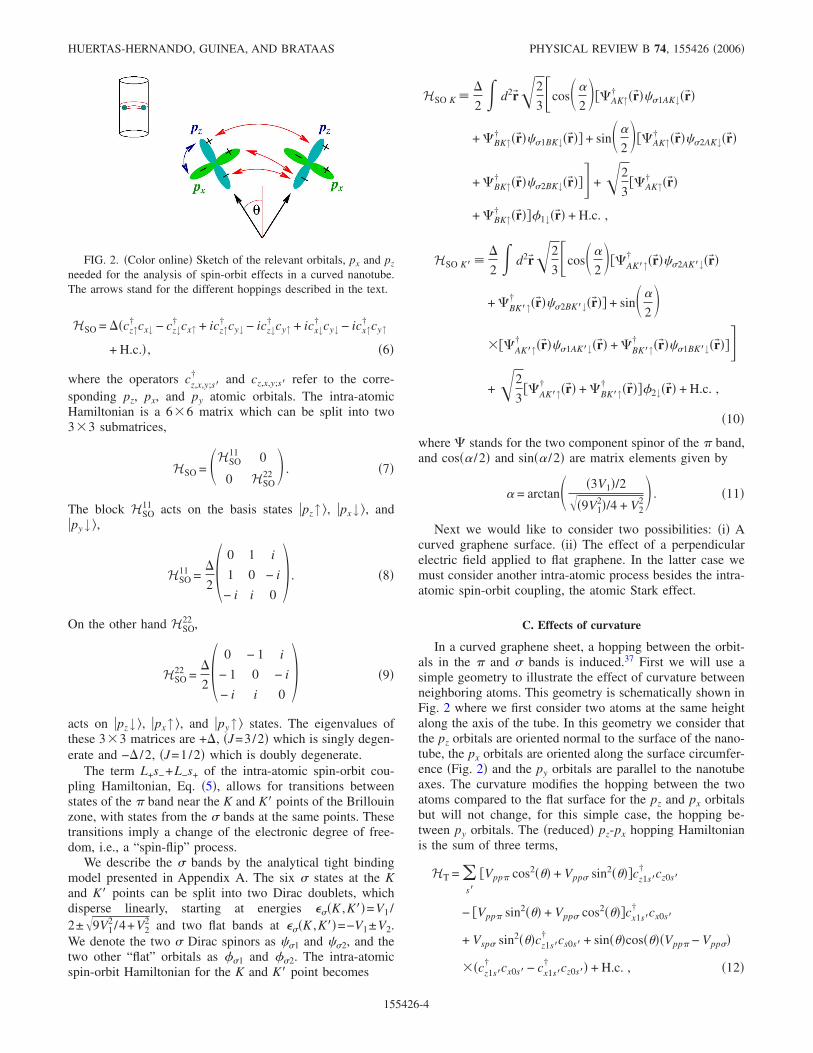
In a curved graphene sheet, a hopping between the orbit-als in the � and � bands is induced.37 First we will use asimple geometry to illustrate the effect of curvature betweenneighboring atoms. This geometry is schematically shown inFig. 2 where we first consider two atoms at the same heightalong the axis of the tube. In this geometry we consider thatthe pz orbitals are oriented normal to the surface of the nano-tube, the px orbitals are oriented along the surface circumfer-ence �Fig. 2� and the py orbitals are parallel to the nanotubeaxes. The curvature modifies the hopping between the twoatoms compared to the flat surface for the pz and px orbitalsbut will not change, for this simple case, the hopping be-tween py orbitals. The �reduced� pz-px hopping Hamiltonianis the sum of three terms,
FIG. 2. �Color online� Sketch of the relevant orbitals, px and pz
needed for the analysis of spin-orbit effects in a curved nanotube.The arrows stand for the different hoppings described in the text.
HUERTAS-HERNANDO, GUINEA, AND BRATAAS PHYSICAL REVIEW B 74, 155426 �2006�
155426-4
where 0 and 1 denote the two atoms considered and � is theangle between the fixed Z axis and the direction normal tothe curved surface �Fig. 2�. The angle �, in the limit when theradius of curvature is much longer than the interatomic spac-ing, aR, is given by ��a /R.
The hopping terms induced by �intrinsic� curvature dis-cussed here break the isotropy of the lattice and lead to aneffective anisotropic coupling between the � and � bands inmomentum space.
The previous discussion can be extended to the case ofgeneral curvature when the graphene sheet has two differentcurvature radii, R1 and R2 corresponding to the x and y di-rections in the plane. In that case, the factor R−1 must bereplaced by R1
−1+R2−1. We now expand on ��a /R1,21. By
projecting onto the Bloch wave functions of the � and �bands at the K and K� points, we find
HTK �Vpp� − Vpp���3
2 a
R1+
a
R2� � d2r��cos�
2�
���AK↑† �r�� �1BK↑�r�� + �BK↑
† �r�� �1AK↑�r��� + sin�
2�
���AK↑† �r�� �2BK↑�r�� + �BK↑
† �r�� �2AK↑�r���� + H.c.
�13�
and a similar expression for the K� point.The induced spin-orbit coupling, however, includes only
contributions from the four � bands at K and K� with ��
=V1 /2±��9V12� /4+V2
2, as those are the only bands coupledto the � band by the intra-atomic spin-orbit term consideredhere, Eq. �10�. We now assume that the energies of the �bands are well separated from the energy of the � bands���=0 at the K and K� points�. Then, we can use second-order perturbation theory and from Eq. �10� and Eq. �13� weobtain an effective Hamiltonian acting on the states of the �band,
Hcurv K� − i��Vpp� − Vpp��V1
2V12 + V2
2 a
R1+
a
R2� � d2r�
���AK↑† �r���BK↓�r�� − �BK↓
† �AK↑� ,
Hcurv K�� − i��Vpp� − Vpp��V1
2V12 + V2
2 a
R1+
a
R2� � d2r�
��− �AK�↓† �r���BK�↑�r�� + �BK�↑
†�AK�↓� .
�14�
D. Effect of an electric field
Now we discuss the atomic Stark effect due to a perpen-dicular electric field E. In this case, we need to consider the�s� orbital of the � bands at each site, and the associatedhopping terms. The Hamiltonian for this case includes thecouplings
HE = �i=1,2;s�=↑,↓
�eEcis;s�† ciz;s� + �scis;s�
† cis;s� + H.c.�
+ Vsp� �s�=↑,↓
�axc1x;s�† c0s;s� + ayc1y;s�
† c0s;s� + H.c.� ,
�15�
where = �pz�z�s� is a electric dipole transition which induceshybridization between the s and pz orbitals and where ax anday are the x and y components of the vector connecting thecarbon atoms 0 and 1. First, we consider the situation ax=1and ay =0. Again Vsp� is the hopping integral between the 2sand 2px ,2py atomic orbitals corresponding to the � band. Wecan now have processes such as
�pz0↑�→E
�s0↑� ——→Vsp�
�px1↑�→�
�pz1↓� ,
�pz0↑�→�
�px0↓� ——→Vsp�
�s1↓�→E
�pz1↓� . �16�
The intermediate orbitals �s0� and �px1� are part of the sigmabands. As before, we describe them using the analytical fit-ting discussed in Appendix A. The �s0� is part of the disper-sive bands, and it has zero overlap with the two nondisper-sive � bands. The processes induced by the electric field, inmomentum space, lead finally to
HEK eE�1
3� d2r��sin�
2���AK↑
† �r�� �1AK↑�r��
+ �BK↑† �r�� �1BK↑�r��� + cos�
2�
���AK↑† �r�� �2AK↑�r�� + �BK↑
† �r�� �2BK↑�r���� + H.c.
�17�
Note that this Hamiltonian mixes the states in the � bandwith states in the � bands which are orthogonal to those inEq. �10�. Combining Eq. �17� and Eq. �10� we obtain, againby second order perturbation theory, an effective Hamil-tonian for the � band
HEK� − i2�2
3
�eEV2
2V12 + V2
2 � d2r�
���AK↑† �r���BK↓�r�� − �BK↓
† �AK↑� ,
HEK�� − i2�2
3
�eEV2
2V12 + V2
2 � d2�r��
��− �AK�↓† �r���BK�↑�r�� + �BK�↑
†�AK�↓� . �18�
The zero overlap between the states in the � bands in Eq.�17� and Eq. �10� imply that only transitions between differ-ent sublattices are allowed.
Defining a 4�4 spinor
SPIN-ORBIT COUPLING IN CURVED GRAPHENE,… PHYSICAL REVIEW B 74, 155426 �2006�
155426-5
�K�K�� =��A↑�r���A↓�r���B↑�r���B↓�r��
K�K��
, �19�
it is possible to join Eqs. �14� and �18� in the followingcompact way:
HRK� = − i�R� d2r��K† ��+s+ − �−s−��K
=�R
2� d2r��K
† ��xsy + �ysx��K, �20�
HRK�� = − i�R� d2r��K�† �− �+s− + �−s+��K�
=�R
2� d2r��K�
† ��xsy − �ysx��K�, �21�
where
�R = �E + �curv,
�E =�V2
2V12 + V2
22�2
3eE� �
2�2
3
�eEV2
,
�curv =�V1
2V12 + V2
2��Vpp� − Vpp�� a
R1+
a
R2��
���Vpp� − Vpp��
V1 a
R1+
a
R2�V1
V2�2
, �22�
where the limit V1V2 �widely separated � bands� has beenconsidered to approximate the above expressions.
Equations �20�–�22� constitute one of the most importantresults of the paper. First, we recover the effective form forthe “Rashba-type” interaction expected from group-theoretical arguments recently.24 Even more importantly, ourresult shows that this effective spin-orbit coupling for the �bands in graphene to first order in the intra-atomic spin-orbitinteraction � is given by two terms.
�i� �E corresponds to processes due to the intra-atomicspin-orbit coupling and the intra-atomic Stark effect betweendifferent orbitals of the � and � bands, together with hop-ping between neighboring atoms. The mixing between the �and � orbitals occurs between the pz and s atomic orbitalsdue to the Stark effect and between the pz and px,y due tothe atomic spin-orbit coupling �. This contribution is theequivalent, for graphene, to the known Rashba spin-orbitinteraction31 and it vanishes at E=0.
�ii� �curv corresponds to processes due to the intra-atomicspin-orbit coupling and the local curvature of the graphenesurface which couples the � and � bands, together with hop-ping between neighboring atoms. The mixing between the� and � orbitals in this case occurs between pz and px,yatomic orbitals both due to the atomic spin-orbit coupling �and due to the curvature. This process is very sensitive todeformations of the lattice along the bond direction between
the different atoms where the p part of the sp2 orbitals isimportant.
E. Intrinsic spin-orbit coupling
We can extend the previous analysis to second order inthe intra-atomic spin-orbit interaction �. We obtain effectivecouplings between electrons with parallel spin. The couplingbetween first nearest neighbors can be written as
�pz0↑��→�
�px0↓�→V�
�px1↓�→�
�pz1↑� ,
�pz0↑�→�
−1
2�px0↓� +
�3
2�py0↓�→
V� 1
2�px2↓� −
�3
2�py2↓�
→�
�pz2↑� ,
�pz0↑�→�
−1
2�px0↓� −
�3
2�py0↓�→
V� 1
2�px3↓� +
�3
2�py3↓�
→�
�pz3↑� , �23�
where the label 0 stands for the central atom. These threecouplings are equal, and give a vanishing contribution at theK and K� points. The intrinsic spin-orbit coupling vanishesfor hopping between neighboring atoms, in agreement withgroup theoretical arguments.24,29,30 We must therefore go tothe next order in the hopping. Expanding to next nearestneighbors, we find a finite contribution to the intrinsic spin-orbit coupling in a flat graphene sheet, corresponding to pro-cesses shown in Fig. 3.
In this case, both the dispersive and nondispersive bandscontribute to the effective �-� coupling, as schematicallyshown by the different arrows in Fig. 1. In order to estimatequantatively the magnitude of the intrinsic coupling, we con-sider processes represented in Fig. 3, which are second orderin �, in momentum space, finally obtaining
FIG. 3. �Color online� Sketch of the processes leading to aneffective intrinsic term in the � band of graphene. Transitionsdrawn in red �dark gray�, and indicated by SO, are mediated by theintra-atomic spin-orbit coupling.
HUERTAS-HERNANDO, GUINEA, AND BRATAAS PHYSICAL REVIEW B 74, 155426 �2006�
155426-6
HintK�K�� = ±3
4
�2
V1
V14
�V22 − V1
2��2V12 + V2
2�
�� d2r��AK�K��↑† �r���AK�K��↑�r��
− �AK�K��↓† �r���AK�K��↓�r��
− �BK�K��↑† �r���BK�K��↑�r��
+ �BK�K��↓�r���BK�K��↓�r�� , �24�
where the � sign corresponds to K�K��, respectively. Wedefine the intrinsic spin-orbit coupling parameter �int in thelimit V1V2 �widely separated � bands� as
�int =3
4
�2
V1
V14
�V22 − V1
2��2V12 + V2
2��
3
4
�2
V1V1
V2�4
. �25�
Our Hamiltonian, Eq. �24�, is equivalent to the one derivedin Ref. 24,
HTSO intrinsic =� d2r��int�†��z�zsz�� , �26�
where �z= ±1 denotes the K�K�� Dirac point and �= ��K ,�K��
T.
III. NUMERICAL ESTIMATES
We must now estimate �int, �E, and �curv. We have=3ao /Z�0.264 Å,36 where Z=6 for carbon and ao isthe Bohr radius, E�50 V/300 nm,4,24 the atomic spin-orbit splitting for carbon �=12 meV→1.3�102 K,38,39
the energy difference between the �-2pz orbitals and the�-sp2 orbitals ��−����14.26−11.79� eV=2.47 eV, theenergy difference between the 2p and the 2s atomicorbitals �s−�p��19.20−11.79� eV=7.41 eV and the hop-pings between the 2s ,2px ,2py ,2pz orbitals of neighboringatoms as Vsp��4.2 eV, Vss��−3.63 eV, Vpp��5.38 eV,and Vpp��−2.24 eV.40,41 We have V1=2.47 eV and V2=6.33 eV. We estimate �int��3�2 /4V1��V1 /V2�4�0.1�10−5 eV→0.01 K. �int is two orders of magnitude smallerthan the estimate in Ref. 24. The discrepancy seems to arisefirst, because the intrinsic spin-orbit splitting �int estimatedhere is proportional to the square of the intra-atomic spin-orbit coupling �2, instead of being proportional to it, asroughly estimated in Ref. 24. Besides, a detailed descriptionof the � bands is necessary to obtain the correct estimate.Spin-orbit splittings of order 1–2.5 K have been discussed inthe literature for graphite.42 However in graphite, the cou-pling between layers is important and influences the effectivevalue of the spin-orbit splitting, typically being enhancedwith respect to the single layer value.30,43,44
For the other two couplings, we use the full expressionobtained for �E and �curv and not the limiting form V1V2,in order to be as accurate as possible. First, we obtain �E= �2�2/3� �eE�V2 / �2V1
2+V22���0.6�10−5 eV→0.07 K.
This estimate for �E, depends on the external electric fieldchosen. Our estimate, for the same value of the electric field,
is two orders of magnitude bigger than the estimate inRef. 24. So far curvature effects have been excluded. Curva-ture effects will increase the total value for the effectivespin-orbit interaction in graphene. Graphene samples seemto have an undulating surface.14 The ripples observed seemto be several Å height and a few tens nm laterally.14
First we consider the simplest example of a ripple being ahalf-sphere of radius R. The part of the sphere which inter-sects the plane of flat graphene and therefore constitutesthe ripple, is assumed to have a typical height hR so theradius R is roughly of the same order of magnitude of thelateral size in this case. It seems possible to identify ripplesof lateral size in the range 50 nm–100 nm in Ref. 14.Choosing a=1.42 Å and R1�R2�50 nm,14 weobtain �curv= �2a /R� ��Vpp�−Vpp���V1 / �2V1
2+V22���2.45
�10−5 eV→0.28 K. Choosing R1�R2�100 nm we obtain�curv�1.22�10−5 eV→0.14 K. Now we consider a differ-ent model where we assume that the sample has randomcorrugations of height h and length l.13 The graphene surfacepresents then an undulating pattern of ripples of average ra-dius R� l2 /h.13 Choosing l�100 Å and h�10 Å,13 we ob-tain again R�100 nm, which leads to the same value for�curv�1.22�10−5 eV→0.14 K. In any case, it seems clearthat due to curvature effects, the effective spin-orbit couplingin graphene could be higher for curved graphene than forperfectly flat graphene. Moreover, spin-orbit coupling in�curved� graphene would be present even for E=0. A moredetailed discussion and/or study of the local curvature and/orcorrugation of graphene is needed in order to obtain moreaccurate estimates.
To conclude this section we present the effective Hamil-tonian for the � bands of graphene including the spin-orbitinteraction,24
HT =� d2r��†− i�vF��x�x + �z�y�y� + �int��z�zsz�
+�R
2��xsy + �z�ysx��� , �27�
where �vF=�3�oa /2, a�2.46 Å being the lattice constantfor graphene, �o�3 eV the McClure intralayer couplingconstant,30,45 �int�0.01 K, �R=�E+�curv the Rashba-curvature coupling �RCC�, where �E�0.07 K for E�50 V/300 nm and �curv�0.2 K. Table I summarizes themain results obtained in the paper for the effective spin-orbitcouplings in a graphene layer.
IV. APPLICATION TO FULLERENES, NANOTUBESAND FULLERENE CAPS
A. Spherical fullerenes
When topological deformations in the form of pentagonsare introduced in the hexagonal lattice of graphene, curvedstructures form. If 12 pentagons are introduced, the graphenesheet will close itself into a sphere forming the well-knownfullerene structure.46 The usual hexagonal lattice “lives” nowon a sphere and presents topological defects in the form ofpentagons. The continuum approximation to a spherical
SPIN-ORBIT COUPLING IN CURVED GRAPHENE,… PHYSICAL REVIEW B 74, 155426 �2006�
155426-7
fullerene leads to two decoupled Dirac equations in the pres-ence of a fictitious monopole of charge ±3/2 in the center ofthe sphere which accounts for the presence of the 12pentagons.47,48 The states closest to the Fermi level are fourtriplets at �=0. We consider the effect of the spin-orbit cou-pling on these triplets first.
Both the coupling induced by the Rashba-Curvature, Eqs.�20� and �21�, and the intrinsic coupling, Eq. �24�, are writtenin a local basis of wave functions where the spin is orientedperpendicular to the graphene sheet, �� ,� , � ↑ � , �� ,� , � ↓ �.It is useful to relate this local basis with a fixed basis inde-pendent of the curvature. Such relation depends on the cur-vature of the graphene sheet considered. In the case of afullerene the graphene sheet is in a sphere. The details aregiven in Appendix B.
The gauge field associated to the presence of fivefoldrings in the fullerene can be diagonalized using the basis
�AKk�s�r�� = �AKk�s�r�� + i�BK�k�s�r�� ,
�BK�k�s�r�� = − i�BK�k�s�r�� + �AKk�s�r�� . �28�
Equivalent transformation is obtained exchanging A↔B.In this basis, the wave functions of the zero energy states
are47
� + 1sK� � 3
4�cos2�
2�ei� �AK�
i�BK��� � �s� ,
�0sK� � 3
2�sin�
2�cos�
2� �AK�
i�BK��� � �s� ,
�− 1sK� � 3
4�sin2�
2�e−i� �AK�
i�BK��� � �s� ,
� + 1sK�� � 3
4�sin2�
2�ei� �AK�
− i�BK��� � �s� ,
�0sK�� −� 3
2�sin�
2�cos�
2� �AK�
− i�BK��� � �s� ,
�− 1sK�� � 3
4�cos2�
2�e−i� �AK�
− i�BK��� � �s� , �29�
where �AK� and �BK�� are envelope functions associated tothe K and K� points of the Brillouin zone and correspondingto states located at the A and B sublattices, respectively. Notethat, at zero energy, states at K�K�� are only located at sub-lattice A�B� sites. �s� denotes the usual spinor part of thewave function corresponding to the electronic spin s= ↑ ,↓.The Hamiltonian Hint couples orbitals in the same sublatticewhereas HR couples orbitals in different sublattices. So HRhas zero matrix elements between zero energy states, as it
does not induce intervalley scattering, mixing K and K�states.13 In the ��+1↑ � , �+1↓ � , �0↑ � , �0↓ � , �−1↑ � , �−1↓ �� ba-sis, the Hamiltonian for the K point of a fullerene looks like
HS-OintK =�
�int 0 0 0 0 0
0 − �int �2�int 0 0 0
0 �2�int 0 0 0 0
0 0 0 0 �2�int 0
0 0 0 �2�int − �int 0
0 0 0 0 0 �int
.
�30�
The Hamiltonian for K� is HS-O intK� =−HS-O int
K .Diagonalizing the Hamiltonian Eq. �30�, we obtain that
each set of spin degenerate triplets obtained in the absence ofthe spin-orbit interaction split into
� = + �int → ��:� + 1↑�, �− 1↓�,�1
3� + 1↓�
+�2
3�0↑�,�1
3�− 1↑� +�2
3�0↓�� ,
� = − 2�int → �−2�:�2
3� + 1↓� −�1
3�0↑�,�2
3�− 1↑�
−�1
3�0↓�� , �31�
Each of these solutions is doubly degenerate, correspond-ing to the K and K� points. In principle, many-body effectsassociated to the electrostatic interaction can be included byfollowing the calculation discussed in Ref. 49.
B. Spin-orbit coupling in nanotubes
The previous continuum analysis can be extended tonanotubes. We use cylindrical coordinates, z ,�, and, as be-fore, define the spin orientations �↑�, �↓� as parallel and anti-parallel to the z axis. The matrix elements relevant for thisgeometry can be easily obtained from Eq. �B1� in AppendixB, by choosing �=� /2. The eigenstates of the nanotube canbe classified by longitudinal momentum, k, and by their an-gular momentum n, �±,k,n= ±�vF
�k2+n2 /R2, where R is theradius of the nanotube. After integration over the circumfer-ence of the nanotube �d�, the Hamiltonian of a nanotubeincluding spin-orbit interaction is
HUERTAS-HERNANDO, GUINEA, AND BRATAAS PHYSICAL REVIEW B 74, 155426 �2006�
155426-8
HS-O R�A���B��
� = 0 �vF�k − in/R� + �i�R�sz
�vF�k + in/R� − �i�R�sz 0��A��
�B��� , �32�
where the �= ±1 corresponds to the K�K�� Dirac point. Notethe basis states �A�� and �B�� used to define Eq. �32� arespinors in spin subspace where the matrix sz acts on �seeAppendix C for details�. The contribution from the intrinsicspin-orbit �int becomes zero after integrating over the nano-tube circumference �Appendix C�. The spin-orbit termi�R�sz in Eq. �32� is equivalent to the term proportional to�y obtained in Eqs. �3.15� and �3.16� of Ref. 37. It is impor-tant to note that the spin orientations �↑�, �↓� in Eq. �32� aredefined along the nanotube axis, whereas the spin orienta-tions used in Eqs. �3.15� and �3.16� of Ref. 37 are definedperpendicular to the nanotube surface. On the other hand, wedo not find any contribution similar to the term proportionalto �x�r� in Eq. �3.15� and �3.16� in Ref. 37. In any case, suchcontributions are not important as they vanish after integrat-ing over the circumference of the nanotube.37 Besides, ourresults are in agreement with the results obtained in Ref. 50.
The energies near the Fermi level, n=0, are changed bythe spin-orbit coupling, and we obtain
�k = ± ����R�2 + ��vFk�2. �33�
There is an energy gap ��R at low energies, in agreementwith the results in Refs. 37 and 51. The ��R gap originatesas a consequence of the Berry phase gained by the electronand hole quasiparticles after completing a closed trajectoryaround the circumference of the nanotube under the effect ofspin-orbit interaction �R.37 Similarly, �R will give rise to asmall spin splitting for n�0,37,51
�34�For a single wall nanotube of radius R1�6,12, 24 Å and
R2→�, a�1.42 Å and for E=0, we get �R�12,6, 3 K,respectively.
C. Nanotube caps
1. Localized states at zero energy
An armchair �5N�5N� nanotube can be ended by aspherical fullerene cap. The cap contains six pentagons and5N�N+1� /2–5 hexagons. When N=3�M, the nanotube ismetallic. An example of such a fullerene cap is given in Fig.4. The boundary between the semispherical fullerene and thenanotube is a circle �Fig. 5�. The solutions of the continuumequations must be continuous across this boundary, and theymust satisfy the Dirac equations appropriate for the sphere inthe cap and for the torus in the nanotube, respectively.
The boundary of the nanotube in the geometry shown inFig. 5 is a zigzag edge. Hence, zero energy states can bedefined,52,53 which at this boundary will have a finite ampli-tude on one sublattice and zero on the other. There is a zero
energy state, ��n� at this boundary, for each value of theangular momentum around the nanotube n. They decay to-wards the bulk of the nanotube as
�n�z,�,K� = Cein�e−�nz�/R, n � 0,
�n�z,�,K�� = Cein�e−�nz�/R, n � 0, �35�
where we are assuming that the nanotube is in the half spacez�0 �see Fig. 5�.
A zero energy state in the whole system can be defined ifthere are states inside the gap of the nanotube ��R, whichcan be matched to the states defined in Eq. �35�. At theboundary we have �=� /2, cos�� /2�=sin�� /2�=1/�2.
FIG. 4. �Color online� Left, one-fifth of a fullerene cap closingan armchair nanotube. The full cap is obtained by gluing five tri-angles like the one in the figure together, forming a pyramid. Apentagon is formed at the apex of the pyramid, from the five tri-angles like the one shaded in green �gray� in the figure. The edgesof the cap are given by the thick black line. The cap contains sixpentagons and 70 hexagons, and it closes a 25�25 armchair nano-tube. Right, sketch of the folding procedure of a flat honeycomblattice needed to obtain an armchair nanotube capped by a semi-spherical fullerene.
SPIN-ORBIT COUPLING IN CURVED GRAPHENE,… PHYSICAL REVIEW B 74, 155426 �2006�
155426-9
Hence, we can combine states �ls K� and �ls K��, l= ±1 inEq. �29� in such a way that the amplitude at the boundary ona given sublattice vanishes,
� + 1s�A 1�2
�� + 1sK� + � + 1sK���
=� 3
8�ei��AK�
0� � �s� ,
�− 1s�A 1�2
��− 1sK� + �− 1sK���
=� 3
8�e−i��AK�
0� � �s� ,
� + 1s�B 1�2
�� + 1sK� − � + 1sK���
=� 3
8�ei� 0
i�BK��� � �s� ,
�− 1s�B 1�2
��− 1sK� − �− 1sK���
=� 3
8�e−i� 0
i�BK��� � �s� . �36�
These combinations match the states decaying into thenanotube, Eq. �35�. This fixes the constant C in Eq. �35� tobe C=�3/ �8��. Note that the wave functions with l=0 canonly be matched to states that do not decay into the bulk ofthe nanotube, i.e., with n=0.
Thus, there are two states per spin s, �+1s�, �−1s�, local-ized at the cap and with finite chirality, n= ±1. A sketchof this procedure is shown in Fig. 5. This continuumapproximation is in general agreement with the results inRef. 54.
As in the case of a spherical fullerene, only the intrinsicspin-orbit coupling mixes these states. The energies of the�±1s�A states are not affected by �int, as the contribution
from �+1s�, is canceled by the contribution from �−1s�. Onthe other hand, the states �±1s�B split in energy, as the�+1s� and �−1s� contributions add up,
� + 1,s = ↑,↓�B → �↑,↓ = ± �int,
�− 1,s = ↑,↓�B → �↑,↓ = � �int. �37�
Note that each state has a finite chirality.
2. Localized states induced by the spin-orbit interaction
The remaining states of a spherical fullerene have multi-plicity 2l+1, where l�2 and energy �l= ±�vF /R�l�l+1�−2. The angular momentum of these states along agiven axis, m, is −l�m� l. The subbands of the nanotubewith angular momentum ±m, have gaps within the energyinterval −�m=−�vF�m� /R����m=vF�m� /R. Thus, there isa fullerene eigenstate with l=2 and angular momentum m= ±2 which lies at the gap edge of the nanotube subbandswith the same momentum. The fullerene state is
i�1 + cos����2�K� + i sin����1 + cos�����K��� , �38�
which can be matched, at �=� /2, to the nanotube eigenstate,
�m=2�z,�� 1
4�2�e2i� �K� − �K��
i�K� + i�K��� . �39�
The spin-orbit coupling acts as a position dependent potential on this state, and it shifts its energy into the m=2 subgap,leading to the formation of another localized state near the cap.
In the following, we consider only the RCC �R. In order to analyze the extension of the state, we assume that the localizedstate decays in the nanotube, z�0 as
FIG. 5. �Color online� �Up� Sketch of the matching scheme usedto build a zero energy state at a fullerene cap. �Down� The wavefunction is one-half of a zero energy state at the cap, matched to adecaying state towards the bulk of the nanotube. See text for details.
HUERTAS-HERNANDO, GUINEA, AND BRATAAS PHYSICAL REVIEW B 74, 155426 �2006�
155426-10
�m=2�z,�� C
4�2�e2i�e�z/R �K� − �K��
i�K� + i�K��� . �40�
We match this wave function to that in Eq. �39� multiplied bythe same normalization constant, C. We assume that the stateis weakly localized below the band edge, so that the mainpart of the wave function is in the nanotube, and �1. Then,we can neglect the change in the spinorial part of the wavefunction, and we will fix the relative components of the twospinors as in Eq. �39� and Eq. �40�. The normalization of thetotal wave function implies that
C−2 =13
16+
1
4�, �41�
where the first term on the right-hand side �rhs� comes fromthe part of the wave function inside the cap, Eq. �39�, and thesecond term is due to the weight of the wave function insidethe nanotube, Eq. �40�. As expected, when the state becomesdelocalized, �→0, the main contribution to the normaliza-tion arises from the “bulk” part of the wave function.
The value of � is fixed by the energy of the state,
�2 = n2 −�2R2
��vF�2 , �42�
where the energy of the state � is inside the subgap �m of thenanotube because of the shift induced by the spin-orbit inter-action �R.
We now calculate the contribution to the energy of thisstate from the RCC, which is now finite, as this state hasweight on the two sublattices,
�Rashba � ± C2�R 1
16�+
31
80� � ±
�R
41 −
59�
20� .
�43�
The rhs of Eq. �43� can be described as the sum of a bulkterm, ±�R /4, and a term due to the presence of the cap,whose weight vanishes as the state becomes delocalized, �→0. The absolute value of the Rashba-curvature contribu-tion is reduced with respect to the bulk energy shift, whichimplies that the interaction is weaker at the cap.
The bulk nanotube bands are split into two spin subbandswhich are shifted in opposite directions. The surface statesanalyzed here are shifted by a smaller amount, so that thestate associated to the subband whose gap increases does notoverlap with the nanotube continuum. Combining the esti-mate of the energy between the gap edge and the surfacestate in Eq. �43� and the constraint for � in Eq. �42�, we find
� �59�RR
20�vF. �44�
Finally, the separation between the energy of the state andthe subgap edge is
� ��vF�2
8R. �45�
For a C60 fullerene of radius R�3.55 Å we obtain, for E=0, a value �R /4�3 K. This effect of the spin-orbit inter-action can be greatly enhanced in nanotube caps in an exter-nal electric field, such as those used for field emissiondevices.55 In this case, spin-orbit interaction may allow forspin-dependent field emission of such devices. The appliedfield also modifies the one electron states, and a detailedanalysis of this situation lies outside the scope of this paper.
V. CONCLUSIONS
We have analyzed the spin-orbit interaction in grapheneand similar materials, like nanotubes and fullerenes. We haveextended previous approaches in order to describe the effectof the intra-atomic spin-orbit interaction on the conduction �and valence � bands. Our scheme allows us to analyze, onthe same footing, the effects of curvature and perpendicularapplied electric field. Moreover, we are able to obtain realis-tic estimates for the intrinsic �int and Rashba-curvature �R=�E+�curv effective spin-orbit couplings in graphene. Wehave shown that spin-orbit coupling for flat graphene israther weak �int�10 mK and �E�70 mK for E=50 V/300 nm. Moreover curvature at the scale of the dis-tance between neighboring atoms increases the value of thespin-orbit coupling in graphene �curv��E��int. This is be-cause local curvature mixes the � and � bands. Graphenesamples seem to have an undulating surface.14 Our estimatefor the typical observed ripples indicates that �curv could beof order �0.2 K. A more detailed study of the curvature ofgraphene samples is needed in order to obtain a more preciseestimate. We conclude that the spin-orbit coupling �R ex-pected from symmetry arguments,24 has a curvature-intrinsicpart besides the expected Rashba coupling due to an electricfield �R=�E+�curv. Therefore �R can be higher for curvedgraphene than for flat graphene. �curv is in a sense a “intrin-sic and/or topological” type of spin-orbit interaction ingraphene which would be present even if E=0, as long as thesamples present some type of corrugation. One importantquestion now is how these ripples could affect macroscopicquantities. It has been already suggested that these ripplesmay be responsible for the lack of weak �anti�localization ingraphene.13,14 Other interesting macroscopic quantities in-volving not only the pseudospin but also the electronic spinmay be worth investigation. These issues are beyond thescope of the present paper and will be subject of future work.
It is also noteworthy that our estimates �R��int, is oppo-site to the condition �R�int obtained by Kane and Mele24
to achieve the quantum spin Hall effect in graphene. So thequantum spin Hall effect may be achieved in neutralgraphene �E=0� only below �0.01 K and provided thesample is also free of ripples so the curvature spin-orbit cou-pling �curv�int. Further progress in sample preparationseems needed to achieve such conditions although some pre-liminary improvements have been recently reported.14 More-over, corrugations in graphene could be seen as topologicaldisorder. It has been shown that the spin Hall effect surviveseven if the spin-orbit gap �int is closed by disorder.26 A de-tailed discussion of the effect of disorder on the other twospin-orbit couplings �E, �curv will be presented elsewhere.
SPIN-ORBIT COUPLING IN CURVED GRAPHENE,… PHYSICAL REVIEW B 74, 155426 �2006�
155426-11
The continuum model derived from microscopic param-eters has been applied to situations where also long rangecurvature effects can be significant. We have made estimatesof the effects of the various spin-orbit terms on the low en-ergy states of fullerenes, nanotubes, and nanotube caps. Forboth nanotubes and nanotube caps we find that �R�1 K. Fornanotubes we have clarified the existent discussion and re-produced the known appearance of a gap for the n=0 statesand spin-splitting for n�0 states in the energy spectrum. Fornanotube caps states, we obtain indications that spin-orbitcoupling may lead to spin-dependent emission possibilitiesfor field-effect emission devices. This aspect will be investi-gated in the future.
Note added. At the final stages of the present paper, tworeports32,33 have appeared. In these papers similar estimatesfor �int�10−3 meV have been obtained for the intrinsic spin-orbit coupling. Moreover similar discussion for the effect ofa perpendicular electric field has been also discussed in Ref.33. Our approach is similar to that followed in Ref. 33. Thetwo studies overlap and although the model used for the �band differs somewhat, the results are quantitative in agree-ment, �E�10−2 meV.
The two reports32,33 and our work agree in the estimationof the intrinsic coupling, which turns out to be weak at therange of temperatures of experimental interest �note, how-ever, that we do not consider here possible renormalizationeffects of this contribution24,56�.
On the other hand, the effect of local curvature �curv onthe spin-orbit coupling has not been investigated in Refs. 32and 33. We show here that this term �curv is as important as,or perhaps even more important than the spin-orbit couplingdue to an electric field �E for the typical values of E reported.
ACKNOWLEDGMENTS
The authors thank Yu. V. Nazarov, K. Novoselov, L. Brey,G. Gómez Santos, Alberto Cortijo, and Maria A. H. Vozme-diano for valuable discussions. Two of the authors �D.H.-H.and A.B.� acknowledge funding from the Research Councilof Norway, through Grant Nos. 162742/v00, 1585181/431,and 1158547/431. One of the authors �F.G.� acknowledgesfunding from MEC �Spain� through Grant No. FIS2005-05478-C02-01 and the European Union Contract No. 12881�NEST�.
APPENDIX A: TWO PARAMETER ANALYTICAL FIT TOTHE SIGMA BANDS OF GRAPHENE
A simple approximation to the sigma bands of graphenetakes only into account the positions of the 2s and 2p atomiclevels, �s and �p, and the interaction between nearest neigh-bor sp2 orbitals. The three sp2 orbitals are
�1� 1�3
��s� + �2�px�� ,
�2� 1�3��s� + �2−
1
2�px� +
�3
2�py��� ,
�3� 1�3��s� + �2−
1
2�px� −
�3
2�py��� . �A1�
The two hopping elements considered are
V1 = ��i�Hatom�j��i�j =�s − �p
3,
V2 = ��i,m�Hhopping�i,n��m,n:nearest neighbors
=Vss� + 2�2Vsp� + 2Vpp�
3, �A2�
where i , j=1,2 ,3 denote “bonding” sp2 states and n ,m de-note atomic sites. V1 depends on the geometry and/or anglebetween the bonds at each atom and V2 depends on the co-ordination of nearest neighbors in the lattice. V1 and V2therefore determine the details of band structure for the �bands.34 The energy associated with each “bonding” state�i�Hatom�i��i=1,2,3�= ��s+2�p� /3 is an energy constant indepen-dent of these details and not important for our discussionhere.
We label a1 ,a2 ,a3 the amplitudes of a Bloch state onthe three orbitals at a given atom, and �b1 ,b2 ,b3� ,�b1� ,b2� ,b3�� , �b1� ,b2� ,b3�� the amplitudes at its three nearestneighbors. These amplitudes satisfy
�a1 = V1�a2 + a3� + V2b1,
�a2 = V1�a1 + a3� + V2b2�,
�a3 = V1�a1 + a2� + V2b3�,
�b1 = V1�b2 + b3� + V2a1,
�b2� = V1�b1� + b3�� + V2a2,
�b3� = V1�b1� + b2�� + V2a3. �A3�
We can define two numbers, an=a1+a2+a3 and bn=b1+b2�+b3� associated to atom n. From Eq. �A3� we obtain
�� − 2V1�an = V2bn,
�� + V1�bn = V2an + V1 �n�;n.−n.
an�, �A4�
where �n�;n−nan�= �b1+b2+b3�+ �b1�+b2�+b3��+ �b1�+b2�+b3��and n−n denotes nearest neighbors.
This equation is equivalent to
� − 2V1 −V2
2
� + V1�an =
V1V2
� + V1�
n�;n.−n.
an�. �A5�
Hence, the amplitudes an satisfy an equation formally iden-tical to the tight binding equations for a single orbital model
HUERTAS-HERNANDO, GUINEA, AND BRATAAS PHYSICAL REVIEW B 74, 155426 �2006�
155426-12
with nearest-neighbor hoppings in the honeycomb lattice. Inmomentum space, we can write
and a�1 ,a�2 are the unit vectors of the honeycomb lattice.The derivation of Eq. �A6� assumes that an�0. There are
also solutions to Eqs. �A3� for which an=0 at all sites. Thesesolutions, and Eq. �A6� lead to
�k =V1
2±�9V1
2
4+ V2
2 ± V1V2fk� ,
�k = − V1 ± V2. �A8�
These equations give the six � bands used in the main text.In order to calculate the effects of transitions between the
� band and the � band on the spin-orbit coupling, we alsoneed the matrix elements of the spin-orbit interaction at thepoints K and K�. At the K point, for instance, the Hamil-tonian for the � band is
H�K �0 V1 V1 V2 0 0
V1 0 V1 0 V2e2�i/3 0
V1 V1 0 0 0 V2e4�i/3
V2 0 0 0 V1 V1
0 V2e4�i/3 0 V1 0 V1
0 0 V2e2�i/3 V1 V1 0
.
�A9�
The knowledge of the eigenstates, Eq. �A5� allows us toobtain also the eigenvalues of Eq. �A9�. The spin-orbit cou-pling induces transitions from the �K ,A , ↑ � state to the sigmabands with energies V1±V2 and spin-down, and from the�K ,A , ↓ � state to the sigma bands with energies
V1 /2±��9V12� /4+V2
2 and spin-up. The inverse processes areinduced for Bloch states localized at sublattice B.
In the limit V1V2, the � bands lie at energies ±V2, withcorrections associated to V1. The spin-orbit coupling inducestransitions to the upper and lower bands, which tend to can-cel. In addition, the net effective intrinsic spin-orbit couplingis the difference between the corrections to the up-spin bandsminus those for the down-spin bands. The final effect is thatthe strength of the intrinsic spin-orbit coupling scales as��2 /V1��V1 /V2�4 in the limit V1V2.
APPENDIX B: MATRIX ELEMENTS OF THE SPIN-ORBITINTERACTION IN A SPHERE
Both the coupling induced by the curvature, Eqs. �20� and�21�, and the interinsic coupling, Eq. �24� can be written, ina simple form, in a local basis of wave functions where thespin is oriented perpendicular to the graphene sheet,�� ,� , � ↑ � , �� ,� , � ↓ �. Using spherical coordinates, � and �the basis where the spins are oriented parallel to the z axis,�↑ � , �↓ �, can be written as
�↑� cos�
2�ei�/2��,�, � ↑� − sin�
2�e+i�/2��,�, � ↓� ,
�↓� sin�
2�e−i�/2��,�, � ↑� + cos�
2�e−i�/2��,�, � ↓� ,
�B1�
where the states �+ � and �−� are defined in terms of somefixed frame of reference. From this expression, we find in thebasis ��A↑ � , �A↓ � , �B↑ � , �B↓ �, basis for K,
HS-OK =�
�int cos��� �int sin���e−i� + i�R sin�
2�cos�
2� − i�R cos2�
2�e−i�
�int sin���ei� − �int cos��� + i�R sin2�
2�e+i� − i�R sin�
2�cos�
2�
− i�R sin�
2�cos�
2� − i�R sin2�
2�e−i� − �int cos��� − �int sin���e−i�
+ i�R cos2�
2�ei� + i�R sin�
2�cos�
2� − �int sin���ei� �int cos���
�B2�
and for K�,
SPIN-ORBIT COUPLING IN CURVED GRAPHENE,… PHYSICAL REVIEW B 74, 155426 �2006�
155426-13
HS-OK� =�
− �int cos��� − �int sin���e−i� − i�R sin�
2�cos�
2� − i�R sin2�
2�e−i�
− �int sin���ei� �int cos��� + i�R cos2�
2�e+i� + i�R sin�
2�cos�
2�
+ i�R sin�
2�cos�
2� − i�R cos2�
2�e−i� �int cos��� �int sin���e−i�
+ i�R sin2�
2�ei� − i�R sin�
2�cos�
2� �int sin���ei� − �int cos���
. �B3�
APPENDIX C: MATRIX ELEMENTS OF THE SPIN-ORBIT INTERACTION IN A CYLINDER
The previous continuum analysis can be extended to nanotubes. We use cylindrical coordinates, z ,�, and, as before, definethe spin orientations �↑ � , �↓ � as parallel and antiparallel to the z axis. The matrix elements can be obtained in a similar way toEq. �B3� by choosing �=� /2,
HS-OK =�
0 �inte−i� + i�R/2 − i�R/2e−i�
�intei� 0 + i�R/2e+i� − i�R/2
− i�R/2 − i�R/2e−i� 0 − �inte−i�
+ i�R/2ei� + i�R/2 − �intei� 0
�C1�
and for K�
HS-OK� =�
0 − �inte−i� − i�R/2 − i�R/2e−i�
− �intei� 0 + i�R/2e+i� + i�R/2
+ i�R/2 − i�R/2e−i� 0 �inte−i�
+ i�R/2ei� − i�R/2 �intei� 0
. �C2�
After integrating over the nanotube circumference �d� the Hamiltonian above becomes
HS-OK =�
0 0 + i�R� 0
0 0 0 − i�R�
− i�R� 0 0 0
0 + i�R� 0 0 �C3�
and for K�
HS-OK� =�
0 0 − i�R� 0
0 0 0 + i�R�
+ i�R� 0 0 0
0 − i�R� 0 0 . �C4�
1 P. R. Wallace, Phys. Rev. 71, 622 �1947�.2 J. C. Slonczewski and P. R. Weiss, Phys. Rev. 109, 272 �1958�.3 D. P. DiVincenzo and E. J. Mele, Phys. Rev. B 29, 1685 �1984�.4 K. S. Novoselov, A. K. Geim, S. V. Morozov, D. Jiang, Y. Zhang,
S. V. Dubonos, I. V. Gregorieva, and A. A. Firsov, Science 306,666 �2004�.
5 K. S. Novoselov, A. K. Geim, S. V. Morozov, D. Jiang, M. I.Katsnelson, I. V. Grigorieva, S. V. Dubonos, and A. A. Firsov,Nature �London� 438, 197 �2005�.
6 K. S. Novoselov, D. Jiang, F. Schedin, T. J. Booth, V. V. Khot-
kevich, S. V. Morozov, and A. K. Geim, Proc. Natl. Acad. Sci.U.S.A. 102, 10451 �2005�.
7 Y. Zhang, Y.-W. Tan, H. L. Stormer, and P. Kim, Nature �London�438, 201 �2005�.
8 A. H. C. Neto, F. Guinea, and N. M. R. Peres, Phys. Rev. B 73,205408 �2006�.
9 N. M. R. Peres, F. Guinea, and A. H. Castro Neto, Phys. Rev. B73, 125411 �2006�.
10 V. P. Gusynin and S. G. Sharapov, Phys. Rev. Lett. 95, 146801�2005�.
HUERTAS-HERNANDO, GUINEA, AND BRATAAS PHYSICAL REVIEW B 74, 155426 �2006�
155426-14
11 L. Brey and H. A. Fertig, Phys. Rev. B 73, 195408 �2006�.12 D. V. Khveshchenko, Phys. Rev. Lett. 97, 036802 �2006�.13 A. F. Morpurgo and F. Guinea, cond-mat/0603789, Phys. Rev.
Lett. �to be published�.14 S. Morozov, K. Novoselov, M. Katsnelson, F. Schedin, D. Jiang,
and A. K. Geim, Phys. Rev. Lett. 97, 016801 �2006�.15 E. McCann, K. Kechedzhi, V. I. Fal’ko, H. Suzuura, T. Ando, and
B. L. Altshuler, Phys. Rev. Lett. 97, 146805 �2006�.16 I. L. Aleiner and K. B. Efetov, cond-mat/0607200 �to be pub-
lished�.17 A. Altland, cond-mat/0607247 �to be published�.18 J. Tworzydo, B. Trauzettel, M. Titov, A. Rycerz, and C. W. J.
Beenakker, Phys. Rev. Lett. 96, 246802 �2006�.19 M. I. Katsnelson, K. S. Novoselov, and A. K. Geim, Nat. Phys. 2,
620 �2006�.20 H. Suzuura and T. Ando, Phys. Rev. Lett. 89, 266603 �2002�.21 K. Nomura and A. H. MacDonald, Phys. Rev. Lett. 96, 256602
�2006�.22 M. I. Katsnelson, Eur. Phys. J. B 52, 151 �2006�.23 D. V. Khveshchenko, cond-mat/0607174 �to be published�.24 C. L. Kane and E. J. Mele, Phys. Rev. Lett. 95, 226801 �2005�.25 L. Sheng, D. N. Sheng, C. S. Ting, and F. D. M. Haldane, Phys.
Rev. Lett. 95, 136602 �2005�.26 N. A. Sinitsyn, J. E. Hill, H. Min, J. Sinova, and A. H. Mac-
Donald, Phys. Rev. Lett. 97, 106804 �2006�.27 P. Esquinazi, D. Spemann, R. Höhne, A. Setzer, K.-H. Han, and
T. Butz, Phys. Rev. Lett. 91, 227201 �2003�.28 G. Dresselhaus, Phys. Rev. 100, 580 �1955�.29 J. C. Slonczewski, Ph.D. thesis, Rutgers University, 1955.30 G. Dresselhaus and M. S. Dresselhaus, Phys. Rev. 140, A401
�1965�.31 Y. A. Bychkov and E. I. Rashba, J. Phys. C 17, 6039 �1984�.32 Y. Yao, F. Ye, X.-L. Qi, S.-C. Zhang, and Z. Fang, cond-mat/
0606350 �to be published�.33 H. Min, J. E. Hill, N. Sinitsyn, B. Sahu, L. Kleinman, and A. H.
MacDonald, Phys. Rev. B 74, 165310 �2006�.34 M. F. Thorpe and D. Weaire, Phys. Rev. Lett. 27, 1581 �1971�.35 F. Guinea, J. Phys. C 14, 3345 �1981�.
36 B. H. Braensden and C. J. Joachain, Physics of Atoms and Mol-ecules �Addison-Wesley, New York, 1983�.
37 T. Ando, J. Phys. Soc. Jpn. 69, 1757 �2000�.38 J. Serrano, M. Cardona, and J. Ruf, Solid State Commun. 113,
411 �2000�.39 F. Hermann and S. Skillman, Atomic Structure Calculations
�Prentice-Hall, Englewood Cliffs, NJ, 1963�.40 D. Tománek and S. G. Louie, Phys. Rev. B 37, 8327 �1988�.41 D. Tománek and M. A. Schlüter, Phys. Rev. Lett. 67, 2331
�1991�.42 N. B. Brandt, S. M. Chudinov, and Y. G. Ponomarev, in Modern
Problems in Condensed Matter Sciences, edited by V. M. Agra-novich and A. A. Maradudin �North-Holland, Amsterdam,1988�, Vol. 20.1.
43 J. W. McClure and Y. Yafet, in 5th Conference on Carbon �Per-gamon, University Park, Pennsylvania, 1962�.
44 Y. Yafet, in Solid State Physics, edited by F. Seitz and D. Turnbull�Academic, New York, 1963�, Vol. 14, p. 2.
45 J. W. McClure, Phys. Rev. 108, 612 �1957�.46 H. W. Kroto, J. R. Heath, S. C. O’Brien, R. F. Curl, and R. E.
Smalley, Nature �London� 318, 162 �1985�.47 J. González, F. Guinea, and M. A. Vozmediano, Phys. Rev. Lett.
69, 172 �1992�.48 J. González, F. Guinea, and M. A. H. Vozmediano, Nucl. Phys. B:
Field Theory Stat. Syst. 406[FS], 771 �1993�.49 F. Guinea, J. González, and M. A. H. Vozmediano, Phys. Rev. B
47, 16576 �1993�.50 A. DeMartino, R. Egger, K. Hallberg, and C. A. Balseiro, Phys.
Rev. Lett. 88, 206402 �2002�.51 L. Chico, M. P. López-Sancho, and M. C. Muñoz, Phys. Rev.
Lett. 93, 176402 �2004�.52 K. Wakabayashi and M. Sigrist, Phys. Rev. Lett. 84, 3390 �2000�.53 K. Wakabayashi, Phys. Rev. B 64, 125428 �2001�.54 T. Yaguchi and T. Ando, J. Phys. Soc. Jpn. 70, 1327 �2001�.55 D. S. Novikov and L. S. Levitov, Phys. Rev. Lett. 96, 036402
�2006�.56 J. González, F. Guinea, and M. A. H. Vozmediano, Nucl. Phys. B:
Field Theory Stat. Syst. 424[FS], 595 �1994�.
SPIN-ORBIT COUPLING IN CURVED GRAPHENE,… PHYSICAL REVIEW B 74, 155426 �2006�