Spin-Transfer Switching in Magnetic Multilayers

By

Inti Antonio Nicolas Sodemann Villadiego

FısicoUniversidad Nacional de Colombia 2007

Submitted in Partial Fulfillment of the Requirements

for the Degree of Master of Sciences in

Physics

College of Arts and Sciences

University of South Carolina

2009

Accepted by:

Yaroslaw Bazaliy, Major Professor

James Knight, Second Reader

James Buggy, Interim Dean of the Graduate School

UMI Number: 1463738

INFORMATION TO USERS

The quality of this reproduction is dependent upon the quality of the copy

submitted. Broken or indistinct print, colored or poor quality illustrations and

photographs, print bleed-through, substandard margins, and improper

alignment can adversely affect reproduction.

In the unlikely event that the author did not send a complete manuscript

and there are missing pages, these will be noted. Also, if unauthorized

copyright material had to be removed, a note will indicate the deletion.

______________________________________________________________

UMI Microform 1463738 Copyright 2009 by ProQuest LLC

All rights reserved. This microform edition is protected against unauthorized copying under Title 17, United States Code.

_______________________________________________________________

ProQuest LLC 789 East Eisenhower Parkway

P.O. Box 1346 Ann Arbor, MI 48106-1346

Dedication

A mi Familia

ii

Acknowledgments

There are many people I feel indebted to and I would like to acknowledge their

support during this time at University of South Carolina.

For my advisor Professor Yaroslaw Bazaliy words will be insufficient to express

my immense gratitude. During this time I have undergone a process of scientific and

personal growth, learning from him not only a myriad of things about the physical

phenomena we are studying, but most importantly many invaluable lessons on how

to do research in physics. He is not only a terrific physicist but a great human being

and I have deeply enjoyed being under his advisement during this time.

Professors Alonso Botero, James Knight, Richard Creswick, Pawel Mazur and

Kuniharu Kubodera, have been not only teachers but inspirational figures, which,

with their knowledge and skills, have reminded me that the true learning relation is

not rooted in the formalities of classes and exams but on natural forces embedded in

human nature that keep us always thirsty for knowledge and understanding. I am

happy to have learned from all of them.

I would like to thank as well all the members of the Condensed Matter Group

working in magnetism in the nanoscale, in particular Dr. Samir Garzon whose scien-

tific attitudes have gained my admiration and was always willing to help me solving

problems that I encountered in my research.

For Ari I have no words to express what I feel. Her seemingly limitless amounts of

patience with my addiction to physics are beyond my comprehension. Her company

in these times has been an invaluable asset in this endeavor.

iii

I am greatly thankful to all my friends, Alejandro, Andres, Asami, Blanca, Bochen,

Camila, Julian, Mike, Mauro, Norma, Samir, Sandra, Vladimir, Yunjing, . . . , who

have given me their support and comprehension, and have made this time in Columbia

so enjoyable.

iv

Abstract

We study the spin transfer torque in nanoscale devices containing layers of fer-

romagnetic materials separated by normal metals. This phenomenon, which arises

from the transfer of spin angular momentum of the conduction electrons to the local-

ized electrons in the ferromagnet, can be used to switch the magnetization direction

between different equilibrium orientations corresponding to local minima of magnetic

energy.

We derive a function representing the ability of spin torque to induce switching,

which turns out to be the divergence of the spin transfer torque. This result is applied

to study switching in a bistable metallic nanopillar device.

We also address the question of the stabilization of magnetization directions which

correspond to saddle points of the magnetic energy and find that in the generic case

such stabilization is not possible and the saddles simply merge with stable equilibria

as the current is increased. Nevertheless, under special conditions saddles can be

stabilized by increasing the current either in a process in which they exchange their

stability nature with distant equilibria or in a collision-like process with an approach-

ing stable equilibrium. These processes are illustrated in the spin flip transistor.

v

Contents

Dedication . . . . . . . . . . . . . . . . . . . . . . . . . . . . . . . . . . . . ii

Acknowledgments . . . . . . . . . . . . . . . . . . . . . . . . . . . . . . . iii

Abstract . . . . . . . . . . . . . . . . . . . . . . . . . . . . . . . . . . . . . v

List of Figures . . . . . . . . . . . . . . . . . . . . . . . . . . . . . . . . . vii

Introduction . . . . . . . . . . . . . . . . . . . . . . . . . . . . . . . . . . . 1

Chapter 1. Magnetism in Nanometer Scale Systems . . . . . . . . . 4

1.1. Origin of Ferromagnetism in Transition Metals . . . . . . . . . . . . 4

1.2. Micromagnetic Description of Magnetization Dynamics . . . . . . . . 6

1.3. Spin Transfer Torque . . . . . . . . . . . . . . . . . . . . . . . . . . . 9

1.4. Metallic Nanopillars and Macrospin Model . . . . . . . . . . . . . . . 15

Chapter 2. Spin Transfer Induced Switching . . . . . . . . . . . . . 20

2.1. Linear Stability Analisis and Magnetization Switching . . . . . . . . 20

2.2. Invariant Form of Spin Transfer Switching Condition . . . . . . . . . 25

2.3. Saddle Point Stabilization and Transcritical Bifurcations . . . . . . . 32

Chapter 3. Selected Applications . . . . . . . . . . . . . . . . . . . . 37

3.1. Metallic Nanopillar with In-plane Magnetic Field . . . . . . . . . . . 37

3.2. Spin Flip Transistor . . . . . . . . . . . . . . . . . . . . . . . . . . . 43

Chapter 4. Summary and Conclusions . . . . . . . . . . . . . . . . . . 48

Bibliography . . . . . . . . . . . . . . . . . . . . . . . . . . . . . . . . . . . 51

vi

List of Figures

Figure 1.1 Typical magnetic nanopillar device with ferromagnetic (FM) and

normal metal (NM) layers . . . . . . . . . . . . . . . . . . . . . 10

Figure 1.2 Schematics of the spin transfer mechanism. . . . . . . . . . . . 13

Figure 1.3 Slonczewski spin torque for different electron spin polarizations P . 13

Figure 2.1 Schematics of constant energy trajectories for a typical nanopillar

in the absence of external magnetic field . . . . . . . . . . . . . 22

Figure 2.2 Divergence of spin torque for different electron spin polarizations

P . . . . . . . . . . . . . . . . . . . . . . . . . . . . . . . . . . . 29

Figure 2.3 Critical angle as function of electron spin polarization P . . . . 30

Figure 2.4 Current dependence of equilibrium position φ(ωI) for s directed

exactly (a) or close (b,c) to the saddle point. Dashed lines show

saddles, solid lines show centers. . . . . . . . . . . . . . . . . . 36

Figure 3.1 a) Typical nanopillar device. b) In plane magnetic field configuration.

38

Figure 3.2 Stability diagram for P = 0.7, α = 0.01, ωa/ωp = 0.01 (values of

ωI and ωH are mesured relative to ωp). Stable regions for P and

AP states, bistable region B and precessional cycles C, in terms of

the current ωI and magnetic field ωH (ω∗H/ωa = 0.76). . . . . . 41

Figure 3.3 Spin flip transistor . . . . . . . . . . . . . . . . . . . . . . . . . 43

Figure 3.4 Transcritical bifurcation in the spin flip transistor. (a) The dashed

lines show how the positions of the easy axis equilibria (M1,2)

vii

approach the saddle, S, with increasing current and merge with it

at a critical value given by eq. (78). (b) In-plane directions of s

and h that slightly break the π/2 rotation symmetry. The saddle

merges with one of the centers, while the other one asymptotically

approaches s. (c-e) transformation of the field F during the merger

of the saddle with two centers in case (a). . . . . . . . . . . . . 47

viii

Introduction

Spintronics, a neologism for spin transport electronics, is a term used to describe

an emerging field in physics and engineering which exploits the interplay between spin

dependent transport of electrons in materials and their magnetic properties. Several

studies of spin dependent transport properties had been done before the 80’s but the

main catalyst that fueled an increased involvement in these topics was the discovery of

the Giant Magnetoresistance (GMR) effect by Peter Grunberg et. al. (Binasch et al.,

1989) and Albert Fert et. al. (Baibich et al., 1988), and the subsequent development

of the device known as spin valve by researchers at IBM, succesfuly incorporated in

the read heads of hard disk drives which lead to a tremendous explosion in their

storage capacity. GMR is the increment of the resistivity of a system of metallic

ferromagnetic layers separated by paramagnetic metals when their magnetization is

antiparallel as compared to the resistance for parallel magnetizations, and its origin

is rooted in the spin dependent electron scattering in the multilayers.

In 1996 two independent theoretical studies by Luc Berger (Berger, 1996) and

John Slonczewski (Slonczewski, 1996), predicted that in a structure like those for

which GMR had been observed not only the flow of electrons would be affected by

the relative orientation of the magnetizations of the ferromagnets, but a reciprocal

reaction would accompany this effect consisting of a torque acting on the ferromagnets

trying to change their magnetization directions. This phenomenon, known as spin

transfer torque, would arise as a reaction to the torque that the conduction electrons

experience after entering a ferromagnet with a polarization direction diferent from

that of the local magnetization.

1

Following this prediction the first experimental observations of spin transfer torques

came from resistance changes for current driven magnetic excitations in point contact

devices (Tsoi et al., 1998). Subsequent experimental studies confirmed the existence of

spin torque induced magnetization switching (Sun, 1999; Wegrowe et al., 1999; Myers

et al., 1999). The current controlled magnetization switching openned the possibility

of building a magnetic bit element, in which the spin transfer torque would be the base

for the writing mechanism and the GMR the base for the reading mechanism. One of

the ideas that makes this proposal compelling is that the magnetization state of these

bits can be kept without any external energy source, provided they are suffciently

stable to resist thermal induced switching, and therefore they could be the basis for

a non-volatile magnetic RAM. An even more ingenious spin torque based memory

device, called the racetrack memory, has been proposed by Stuart Parkin (Parkin,

2004; Parkin et al., 2008), which makes use of magnetic domain walls states as bits

which are stored in a long magnetic stripe and the spin transfer induced motion of

the walls is used to shift the bits through the reading and writing elements.

The present work is concerned with the stability of magnetic states and the spin

torque induced switching in magnetic layers whose dimensions are small enough as

to consider them monodomain bodies, these scales are typically 5nm for their thick-

ness and 100nm for their lateral sizes and the theoretical framework employed to

describe them is known as macrospin model. Even though a considerable amount of

theoretical and experimental studies have been done for these systems and a clear

picture of the basic phenomena is currently available, there are important problems

and questions ahead to be solved. From the perspective of applicability to memory

devices, the two main challenges can be sumarized as follows: how to reduce the

critical switching current and consequently the energy dissipated during switching,

and, how to reduce the switching time, these objectives should be met without harm-

ing the inherent magnetic stability of the device to thermal fluctuations. From the

perspective of fundamental understading of spin transfer, several debates are still

2

open, this is particularly related to the fact that the experimental observation of spin

torque related effects is basically confined to resistivity measurements (which can be

related to the relative orientation of the magnetizations in the multilayer system via

the GMR effect), this rather limited access to the state of the system makes difficult

to discriminate between different proposals for the spin transfer efficiency 1.

In this thesis we intend to introduce a function that quantifies the switching

ability of the spin transfer torque in the context of the macrospin model, this quantity

turns out to be the divergence of the spin torque and quantifies the tendency of spin

torque to stabilize/destabilize configurations which are local minima and maxima of

magnetic energy. We also address a relatively less explored scenario, the stabilization

of equilibria corresponding to saddle points of magnetic energy, and find that this can

be accomplished for special configurations.

This work is written in a relatively self contained manner, in the first chapter, I will

introduce the basic theoretical ideas and the model required to describe the system of

our interest, which is a device made of two ferromagnetic layers separated by a metal

spacer through which an electric current is passed, known as metallic nanopillar.

In the second chapter I will introduce the idea of divergence of spin torque as a

measure of its switching ability and discuss the problem of saddle point stabilization

and saddle-center merging, defining the conditions for a particular merging known as

transcritical bifurcation to occur. The third chapter will illustrate the general ideas

introduced in the second one, in particular the nanopillar with an in-plane external

magnetic field will serve as a test for the idea of switching ability of spin torque and

the spin flip transistor will illustrate the saddle point stabilization and transcritical

bifurcations. A final section will close summarizing the main results and conclusions

of this work.

1In magnetic tunnel junctions (ferromagnetic multilayers separated by insulators) the situation ismore complicated because of the strong intrinsic bias dependence of the conductivity, and still acomplete functional form for the spin torque is missing.

3

Chapter 1

Magnetism in Nanometer Scale Systems

1.1. Origin of Ferromagnetism in Transition Metals

The ability of materials to display a macroscopic magnetization in the absence of

externally applied magnetic fields is known as ferromagnetism 1. Ferromagnetism has

its origin in the ordering that the spin of the electrons in these materials collectivelly

develop when the temperature drops below a critical value known as Curie temper-

ature. Below this temperature, the electrons of neighboring ions tend to align their

spins along a common direction, resulting in a local non-vanishing magnetization.

The interaction that underlies this phenomenon is not any explicit spin-dependent

coupling of the electrons, like the dipole-dipole interactions or spin-orbit coupling,

but a cooperation of the usual electrostatic Coulomb repulsion between electrons and

the Pauli exclusion principle, commonly referred to as exchange interaction (Ashcroft

and Mermin, 1976).

This interaction is responsible as well for the presence of spontaneus magnetization

in individual atoms and molecules, in particular an isolated atom with partially filled

orbitals will, in general, have a nonvanishing magnetic moment in its ground state,

as described by Hund’s rules. Nevertheless, this magnetic moment disappears for

most of the materials when the atom is placed in a metallic crystalline environment.

For most metals the appearance of band structure tends to suppress the formation of

magnetic moments, the main reason being the great modifications that the metallic

1This definition encompasses the so-called ferrimagnetic materials, which sometimes are classifiedas a category on its own.

4

phase poses to the electron repulsion, which strongly supresses the exchange inter-

action otherwise present in the free atoms. In spite of this, some transition metals

like iron or cobalt, are able to retain a considerable amount exchange interaction in

the presence of band formation and then constitute examples of metallic ferromag-

nets. The exchange interaction in these materials generates a self consistent shift

of the bands into majority-electron-spin band and minority-electron-spin band each

containing electrons aligned in a common direction with the majority bands having

lower energy (Ralph and Stiles, 2008). This energy difference results in a unbalance

of spin populations which gives rise to a local magnetization.

5

1.2. Micromagnetic Description of Magnetization Dynam-

ics

In a macroscopic sample of ferromagnetic material the magnetization is not uni-

form, but rather it is divided into small regions called magnetic domains in which

the magnetization is approximately uniform, the reason for these nonuniformities is

mainly the dipole coupling that builds up between different regions of the ferromag-

net, this coupling between any two regions favors the antiparallel alignment of their

magnetic moments and therefore competes with the exchange interaction in the larger

scales.

To describe these spatial non-uniformities of the magnetization in a ferromag-

net, that start appearing typically at the scale of 10 - 100 nm, a phenomenological

description, commonly called micromagnetics, is introduced. In this description the

magnetization is represented by a continuous vector field M(r). The free energy func-

tional associated with M(r) can be built by adding up the contributions of different

sources of magnetic energy. These sources are generally four: the interaction with any

external magnetic field, the magnetocrystalline anisotropy energy, the micromagnetic

exchange, and the previously mentioned dipole interaction of the magnetostatic field

generated by M(r) itself (Ralph and Stiles, 2008). The magnetocrystalline anisotropy

energy arises from the spin-orbit coupling and tends to align the magnetization along

particular lattice directions. The micromagnetic exchange is a residual interaction

of the microscopic exchange electron interaction and tends to mantain the direction

of the magnetization uniform in the ferromagnet. The explicit form of the energy

functional containing these interactions 2

2For simplicity we have assumed the magnetocrystalline anisotropy to be uniaxial.

6

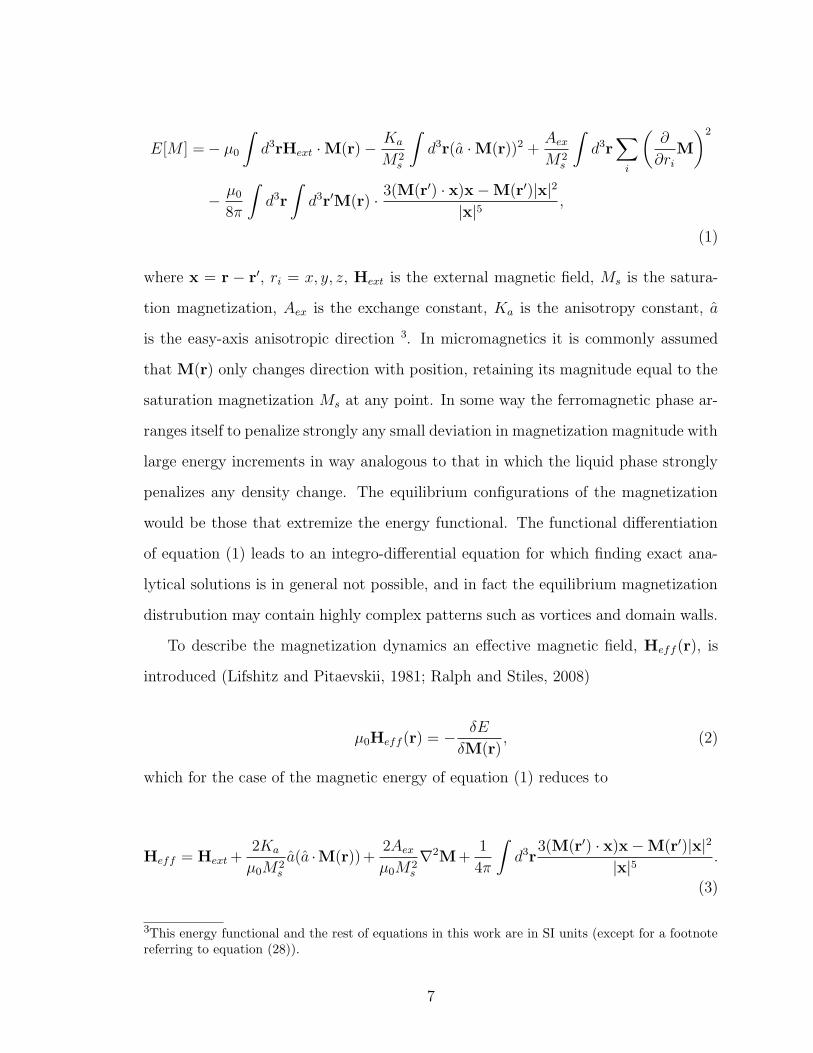
E[M ] = − µ0

∫

d3rHext · M(r) − Ka

M2s

∫

d3r(a · M(r))2 +Aex

M2s

∫

d3r∑

i

(

∂

∂ri

M

)2

− µ0

8π

∫

d3r

∫

d3r′M(r) · 3(M(r′) · x)x − M(r′)|x|2|x|5 ,

(1)

where x = r − r′, ri = x, y, z, Hext is the external magnetic field, Ms is the satura-

tion magnetization, Aex is the exchange constant, Ka is the anisotropy constant, a

is the easy-axis anisotropic direction 3. In micromagnetics it is commonly assumed

that M(r) only changes direction with position, retaining its magnitude equal to the

saturation magnetization Ms at any point. In some way the ferromagnetic phase ar-

ranges itself to penalize strongly any small deviation in magnetization magnitude with

large energy increments in way analogous to that in which the liquid phase strongly

penalizes any density change. The equilibrium configurations of the magnetization

would be those that extremize the energy functional. The functional differentiation

of equation (1) leads to an integro-differential equation for which finding exact ana-

lytical solutions is in general not possible, and in fact the equilibrium magnetization

distrubution may contain highly complex patterns such as vortices and domain walls.

To describe the magnetization dynamics an effective magnetic field, Heff (r), is

introduced (Lifshitz and Pitaevskii, 1981; Ralph and Stiles, 2008)

µ0Heff (r) = − δE

δM(r), (2)

which for the case of the magnetic energy of equation (1) reduces to

Heff = Hext +2Ka

µ0M2s

a(a ·M(r))+2Aex

µ0M2s

∇2M+1

4π

∫

d3r3(M(r′) · x)x − M(r′)|x|2

|x|5 .

(3)

3This energy functional and the rest of equations in this work are in SI units (except for a footnotereferring to equation (28)).

7

This field generates a torque density on the local magnetic moments given by µ0M×

Heff , this torque gives the rate of change for the total angular momentum density of

the electrons in the ferromagnet which is the source of the magnetization M(r). In

the simplest case, and fortunately the most common for the magnetic multilayers of

our interest, the angular momentum density equals the electron spin density, S, and

the rate of change of the magnetization is proportional to the torque density 4

∂tM = −γ0µ0M × Heff , (4)

with γ0 = gµB/~ being the gyromagnetic ratio of the electron, µB the Bohr magneton

and g the g-factor of the electron 5. Equation (4) contains no dissipation, and describes

the precession of M around the effective field Heff . A phenomelogical dissipative

term, known as Gilbert damping, may be added with the resulting equation reading

as

∂tM = −γ0µ0M × Heff +α

Ms

M × ∂tM, (5)

where α is the Gilbert damping parameter, whose value is of the order of 10−3 and

it is dimensionless. Equation (5) is normally referred to as Landau-Lifshitz-Gilbert

equation or simply LLG equation. This equation is the central mathematical object of

this work, by adding a suitable term describing the spin transfer torque we will study

the stabillity properties of different equilibrium configurations for the magnetization

and their dependence on the parameters describing the magnetic interactions of the

system.

4In cases for which the orbital angular momentum plays a role this proportioanlity would be broken,see e.g. Ralph and Stiles (2008).

5This g factor is in general material dependent and may slightly differ from the g factor of theisolated electron.

8

1.3. Spin Transfer Torque

In any metal, either normal or ferromagnetic, an electron spin density, S, with

an associated spin current density, Q, may be introduced. S is a vectorial quantity

whereas Q is a tensor cointaining information about both the direction of the spin

density itself and the direction of its flow. Thus Qij would represent the amount

of jth component of the spin flowing along the ith direction per unit area per unit

time (Stiles and Zangwill, 2002).

In a material in which the electrons have no spin dependent interactions the total

spin is conserved, this can be expressed as a continuity equation for S

∂tS + ∇ · Q = 0, (6)

where ∇ refers to derivatives with respect to the spatial part (as opposed to the spin

part). Nevertheless when spin dependent interactions exist, the spin is no longer

conserved, and terms representing spin “sources” and “sinks” must be added to the

right side of equation (6). If inelastic spin-flip processes are neglected together with

the orbital contribution to the total angular momentum density then the rate of spin

density non-conservation is the torque density, N, and equation (6) reads as

∂tS + ∇ · Q = N. (7)

For a ferromagnetic material, if again orbital angular momentum is neglected, the

spin density is proportional to its local magnetization

M = −γ0S, (8)

the torque density is the same that appears in the right side of LLG equation (5),

therefore equation (7) can be written as:

∂tM = −γ0µ0M × Heff +α

Ms

M × ∂tM + γ0∇ · Q. (9)

9

NM

FM

FM

I

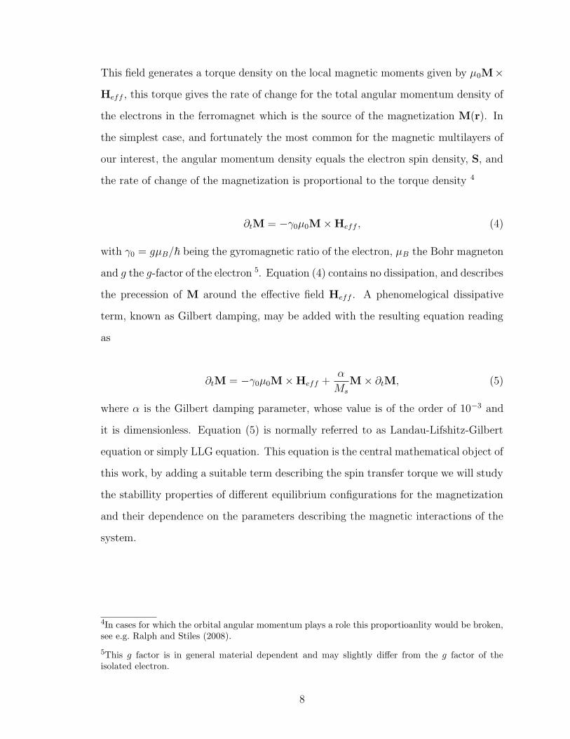
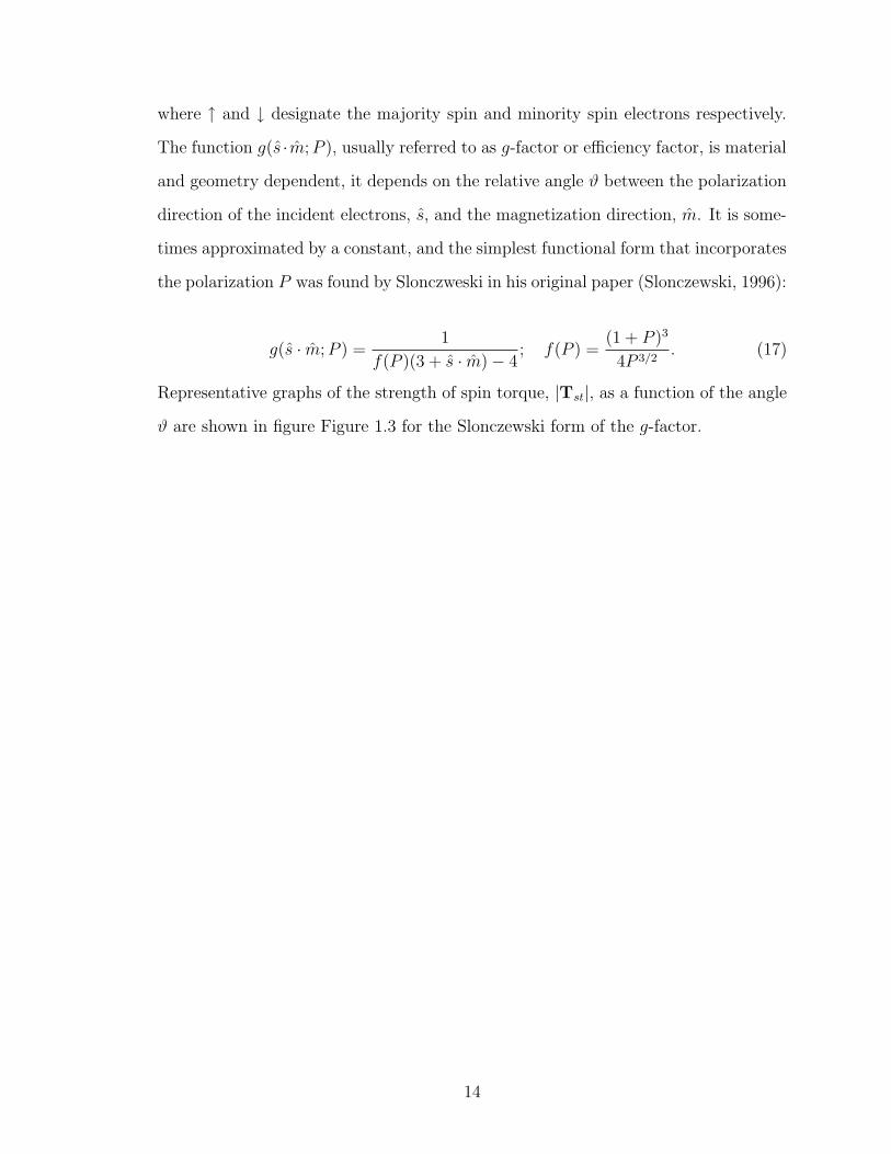
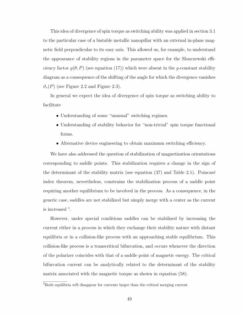
Figure 1.1. Typical magnetic nanopillar device with ferromagnetic(FM) and normal metal (NM) layers

When compared with equation (5) above equation suggests that the term −∇ · Q

might be interpreted as an effective torque acting on M originated from the spin

current flowing through the ferromagnet. We will refer to this term as a torque in the

rest of this work, although we must keep in mind that this is not an actual torque

acting on the spin of electrons itself in the sense defined by equation (7).

The contribution to the rate of change of M from ∇ · Q contains the so-called spin

transfer torque (Slonczewski, 1996; Berger, 1996; Stiles and Zangwill, 2002) and other

spin dependent transport contributions like spin pumping (Tserkovnyak et al., 2002).

To be able to compute the magnetization dynamics from equation (9) it is neces-

sary to explicitly relate Q and M, this requires a theory of spin depenpent electron

transport in the bulk normal and ferromagnetic metals and their interfaces. The

properties of spin transport are structure and material dependent and therefore these

theories need some degree of specialization into particular classes of magnetic struc-

tures and the materials from which they are made. The structures in which we will

focus throughout this work are the metal-ferromagnet multilayers, in particular a

device consisting of a sandwich of ferromagnet-normal metal-ferromagnet known as

metallic nanopillar or spin-valve (see Figure 1.1).

Several theoretical approaches, with similar results, have been employed to com-

pute the spin transfer torque from the spin current in metallic nanopillars 6. Even

6See for example Slonczewski (1996); Bazaliy et al. (1998); Stiles and Zangwill (2002); Xiao et al.(2004); Brataas et al. (2006); Haney et al. (2008).

10

though the details underlying the mechanism are subtle, the basic picture is relatively

simple. Conduction electrons near the Fermi surface are highly movable in the mul-

tilayer. This can be seen as follows: Fermi velocity of conduction electrons is of the

order vF ∼ 106m/s, typical thickness of magnetic layers is d ∼ 10nm, therefore the

time an electron takes to go through the layer is of the order te ∼ 10−14s, on the

other hand the typical magnetization motion time scale is of the order tM ∼ 1ns 7,

thus tM te. This simple observation leads to the important approximation that

for practical purposes the magnatization dynamics can be considered as “frozen” in

order to compute the electron transport properties through the nanopillar.

Another relevant observation is that in order to compute the total spin transfer

torque acting on the ferromagnetic layer, Tst only the values of the spin current at

the interfaces are required, this is readily concluded from Gauss theorem

Tst = γ0

∫

d3r∇ · Q = γ0

∫

dan · Q. (10)

We consider now a simplified version of the toy model for scattering processes

that occur at the normal metal-ferromagnet interface presented by Ralph and Stiles

(2008). Consider a single electron incident from the normal metal into the ferromagnet

with velocity normal to the interface, in such case we need to consider only three

components of the spin current, Qxx, Qyx, Qzx, and in this case Q can be treated as

a vector. Suppose the magnetic moment of the electron points in a direction given by

s (its spin therefore points along −s), in this case the incident spin current density

can be written as

Qinc ∝ − v

V

~

2s, (11)

where v is the velocity of the electron, and V is the volume of the ferromagnetic

layer. When the electron enters the ferromagnet it experiences the strong exchange

7This can be estimated with the frequency parameters that will appear in equation (28).

11

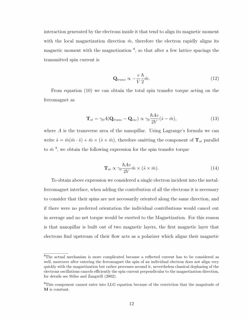
interaction generated by the electrons inside it that tend to align its magnetic moment

with the local magnetization direction m, therefore the electron rapidly aligns its

magnetic moment with the magnetization 8, so that after a few lattice spacings the

transmitted spin current is

Qtrans ∝ − v

V

~

2m. (12)

From equation (10) we can obtain the total spin transfer torque acting on the

ferromagnet as

Tst = γ0A(Qtrans − Qinc) ∝ γ0~Av

2V(s − m), (13)

where A is the transverse area of the nanopillar. Using Lagrange’s formula we can

write s = m(m · s) + m × (s × m), therefore omitting the component of Tst parallel

to m 9, we obtain the following expression for the spin transfer torque

Tst ∝ γ0~Av

2Vm × (s × m). (14)

To obtain above expression we considered a single electron incident into the metal-

ferromagnet interface, when adding the contribution of all the electrons it is necessary

to consider that their spins are not necessarily oriented along the same direction, and

if there were no preferred orientation the individual contributions would cancel out

in average and no net torque would be exerted to the Magnetization. For this reason

is that nanopillar is built out of two magnetic layers, the first magnetic layer that

electrons find upstream of their flow acts as a polarizer which aligns their magnetic

8The actual mechanism is more complicated because a reflected current has to be considered aswell, moreover after entering the ferromagnet the spin of an individual electron does not align veryquickly with the magnetization but rather precesses around it, nevertheless classical dephasing of theelectrons oscillations cancels efficiently the spin current perpendicular to the magnetization direction,for details see Stiles and Zangwill (2002).

9This component cannot enter into LLG equation because of the restriction that the magnitude ofM is constant.

12

M

ms

Polarizer FM NM FM

ϑ

Qinc Qtrans

ϑ

Figure 1.2. Schematics of the spin transfer mechanism.

stτωI

0

0.5

1

3π/4π/2π/40

ϑ

π

P = 0.6

P = 0.4

P = 0.2

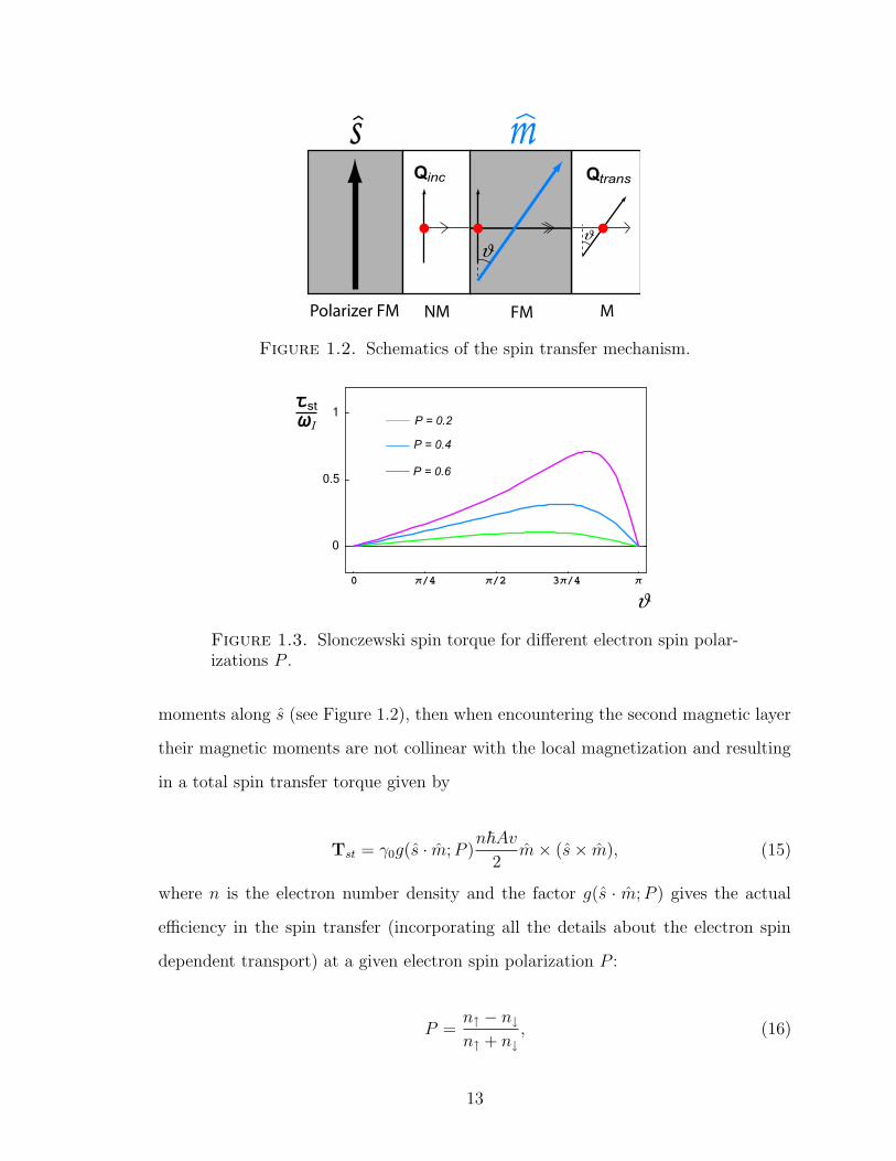
Figure 1.3. Slonczewski spin torque for different electron spin polar-izations P .

moments along s (see Figure 1.2), then when encountering the second magnetic layer

their magnetic moments are not collinear with the local magnetization and resulting

in a total spin transfer torque given by

Tst = γ0g(s · m; P )n~Av

2m × (s × m), (15)

where n is the electron number density and the factor g(s · m; P ) gives the actual

efficiency in the spin transfer (incorporating all the details about the electron spin

dependent transport) at a given electron spin polarization P :

P =n↑ − n↓

n↑ + n↓

, (16)

13

where ↑ and ↓ designate the majority spin and minority spin electrons respectively.

The function g(s ·m; P ), usually referred to as g-factor or efficiency factor, is material

and geometry dependent, it depends on the relative angle ϑ between the polarization

direction of the incident electrons, s, and the magnetization direction, m. It is some-

times approximated by a constant, and the simplest functional form that incorporates

the polarization P was found by Slonczweski in his original paper (Slonczewski, 1996):

g(s · m; P ) =1

f(P )(3 + s · m) − 4; f(P ) =

(1 + P )3

4P 3/2. (17)

Representative graphs of the strength of spin torque, |Tst|, as a function of the angle

ϑ are shown in figure Figure 1.3 for the Slonczewski form of the g-factor.

14

1.4. Metallic Nanopillars and Macrospin Model

Spin torque and spin dependent conductivity phenomena have been observed in

different systems incorporating magnetic, metallic and insulating components. Many

of the basic ideas so far discussed apply to several of these systems, but to further

elaborate the theoretical considerations I will restrict to a more definite class of phys-

ical systems referred to as metallic nanopillar devices 10.

A metallic nanopillar device consists of thin magnetic layer of a soft ferromagnetic

material named free layer typically made of Ni80+δFe20−δ (permalloy) or Co90+δFe10−δ

which has therefore a low coercivity and thus its magnetization is easy to reorient

and a fixed or pinned layer with a high coercivity so that its orientation change is

negligible 11 and serves as the polarizer layer.

The free layer is typically patterned elliptical to produce a preferred axis of ori-

entation for the magnetization, its width is around 100nm and thickness around

5nm. Even though the current perpendicular to plane (CPP) configuration is cus-

tomarily used because of its higher magnetoresistance values, in plane configurations

are also possible. The available techniques for measuring the magnetization dynam-

ics are rather limited and most of them rely in the giant magnetoresistance effect

(GMR) (Baibich et al., 1988; Binasch et al., 1989), which is the dependence of the

resistance of a multilayer sandwich on the relative orientation of the magnetization

of each ferromagnetic layer, in particular for the nanopillar shown in fig. Figure 1.1

the resistance is minimal for parallel magnetizations and maximal for antiparallel

magnetizations.

A continous description of the dynamics of a metallic nanopillar like the ones

previouly described would combine the LLG equation with the spin torque (9), even

10Some of the results I will derive can be applied to moderately modified versions of the metallicnanopillar, like magnetic tunnel junctions and nonlocal spin valves

11This is typically achieved by making the fixed layer much thicker than the free layer, by exchangebiasing the layer with an extra antiferromagnetic layer or by making it much wider than free layer(extended layer) (see eg. Krivorotov et al. (2005); Garzon et al. (2008))

15

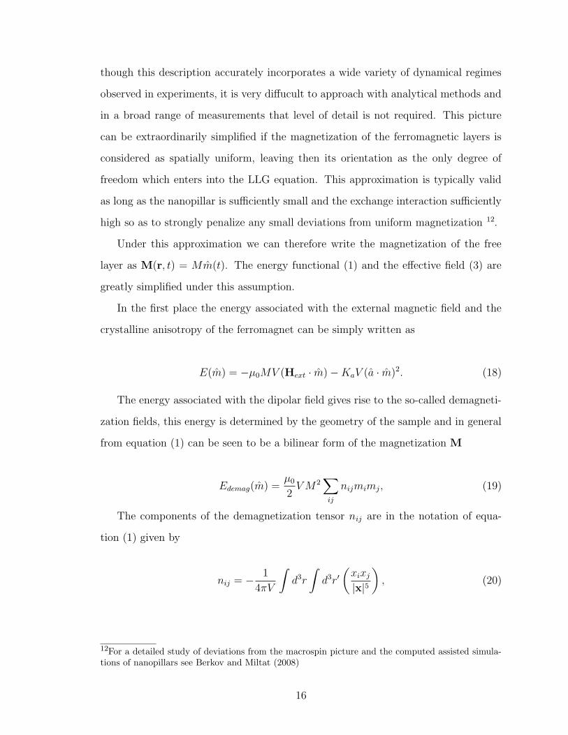
though this description accurately incorporates a wide variety of dynamical regimes

observed in experiments, it is very diffucult to approach with analytical methods and

in a broad range of measurements that level of detail is not required. This picture

can be extraordinarily simplified if the magnetization of the ferromagnetic layers is

considered as spatially uniform, leaving then its orientation as the only degree of

freedom which enters into the LLG equation. This approximation is typically valid

as long as the nanopillar is sufficiently small and the exchange interaction sufficiently

high so as to strongly penalize any small deviations from uniform magnetization 12.

Under this approximation we can therefore write the magnetization of the free

layer as M(r, t) = Mm(t). The energy functional (1) and the effective field (3) are

greatly simplified under this assumption.

In the first place the energy associated with the external magnetic field and the

crystalline anisotropy of the ferromagnet can be simply written as

E(m) = −µ0MV (Hext · m) − KaV (a · m)2. (18)

The energy associated with the dipolar field gives rise to the so-called demagneti-

zation fields, this energy is determined by the geometry of the sample and in general

from equation (1) can be seen to be a bilinear form of the magnetization M

Edemag(m) =µ0

2V M2

∑

ij

nijmimj, (19)

The components of the demagnetization tensor nij are in the notation of equa-

tion (1) given by

nij = − 1

4πV

∫

d3r

∫

d3r′(

xixj

|x|5)

, (20)

12For a detailed study of deviations from the macrospin picture and the computed assisted simula-tions of nanopillars see Berkov and Miltat (2008)

16

where an irrelevant term proportional M 2 has been already omitted. We will not

concern ourselves into computing the exact form of the demagnetization tensor in

terms of the geometric parameters of a nanopillar (the derivation for an ellipsoid can

be found in Landau and Lifshitz (1984)). For the thin planar elliptical nanopillar typ-

ically two terms appear, one usually called easy plane anisotropy which incorporates

the fact that orientations out of the plane are less favorable energetically, and the

second one, the easy axis anisotropy expresses the preference of the magnetization to

lie parallel to the long axis of the ellipse. With this the anisotropic demagnetization

energy can be written as 13

Edemag(m) =µ0

2V M2(m · p)2 − µ0

2V MHK(m · a)2, (21)

with p the unit vector normal to the easy plane of the nanopillar and a the vector

along the easy axis. Generally this axis is chosen to coincide with one of the crystalline

axis of the ferromagnet 14, in this case the easy axis anisotropy field strength HK15

can be thought as containing both, contributions from shape and intrinsic anisotropy,

then we can write the total magnetic energy of the nanopillar as,

E(m) =µ0

2V M2(m · p)2 − µ0

2V MHK(m · a)2 − µ0MV (Hext · m). (22)

It is worth mentioning that the external magnetic field may contain not only

the externally applied magnetic field to the free layer of the nanopillar but also any

field coming from the dipolar coupling with the fixed layer or even terms that are

not strictly speaking magnetic fields but that have the same functional form in the

13The easy plane anisotropy can be easily shown to have this form for an infinitesimally thin nanopil-lar using the notion of solid angle of a surface Ω =

∫

Sx·n|x|2 da.

14The crystalline anisotropy is typically much smaller than the demagnetization anisotropy associ-ated to the shape of the sample for typicall metallic ferromagnets.

15HK is defined as the strength of the critical magnetic field required to produce magnetic switchingwhen applied in the direction of the easy axis of the nanopillar and usually referred to as Stoner-Wolfarth switching field.

17

contribution to the magnetic energy like the exchange coupling between the fixed

layer and the free layer through the intermediate metallic spacer 16.

The effective magnetic field can then be computed by the anologue to equation (2),

where now the derivative with respect the magnetic moment µ = V M needs to be

computed, in this case the effective field can be found from

Heff (m) = − 1

µ0V M

∂E

∂m, (23)

thus from equation (22), the effective field is

Heff (m) = −Mp(p · m) + HK a(a · m) + Hext. (24)

On the other equation (9) can be written in this case as

dm

dt= −γ0µ0m × Heff + αm × dm

dt+

1

MVTst, (25)

by replacing the explicit form of Tst from eq. (15) we obtain the LLG equation for

the magnetization direction of a single domain nanopillar under the influence of spin

torque,

dm

dt= heff × m + αm × dm

dt+ ωIg(m · s)m × (s × m), (26)

where heff = γ0µ0Heff explicitly reads as:

heff = ωaa(m · a) − ωpp(m · p) + ωH h, (27)

where h is the unit vector along the external magnetic field Hext. All the ω’s constants

have units of frequency and can be explicitly related to the previously introduced

constants by:

16Exchange coupling is an interaction between the magnetizations of different layers in multilayersstacks which originates in the spin dependent “trapping” of the electrons in the intermediate non-magnetic spacers which has a form Jexs · m, where the sign of Jex has oscillatory behavior with thespacer thickness (see eg. Parkin et al. (1990); Bruno and Chappert (1991)).

18

ωp = γ0µ0M, ωa = γ0µ0HK , ωH = γ0µ0Hext, ωI = γ0~jA

2MV e, (28)

where j = nev is the electric current density 17. The fact that all the constants in

the LLG equation (27) have units of frequency makes straightforward the comparison

between strength of terms with different origins 18.

Equation (27) will be the starting point of the rest of work where we will address

the question of how the dynamics of the magnetization of the free layer of a sufficiently

small nanopillar is modified in the presence of the spin transfer torque.

17Strictly speaking j is minus the electric current density and is positive when the electrons flowfrom the fixed to the free layer

18In Gaussian units these constants are: ωp = γ4πM , ωa = γHK , ωH = γH and ωI = γ ~jA2MV e

; thegyromagnetic ratio in gaussian units γ is related to that in SI units by γ = cγ0.

19

Chapter 2

Spin Transfer Induced Switching

2.1. Linear Stability Analisis and Magnetization Switching

Equation (27) describes the variation of a unit vector m along the magnetization

of the free layer of a nanopillar, therefore, its associated configuration space is the

unit bidimensional sphere S2. In the present work we will restrict to cases for which

the parameters in this equation do not change with time, this precludes the possibility

of chaotic dynamics (Bonin et al., 2007). The consistency of this fact is ensured by

the condition

m · dm

dt= 0, (29)

which implies that the norm of the vector m is preserved by the dynamics. By taking

the cross product of LLG equation (27) with m on both sides we can rewrite it as

follows,

(1 + α2)dm

dt= F(m) ≡ τ (m) + αm × τ (m) , (30)

where τ is the sum of the torques coming from the effective magnetic field (which we

call conservative torque τ c) and the spin torque (which we call τ st)

τ = τ c + τ st. (31)

The factor (1 + α2) in equation (30) can be eliminated by rescaling time t′ =

t/(1 + α2), rendering this equation to the simple form 1

1we will drope the prime from t′ in all the remaining discussion

20

dm

dt= F(m). (32)

Above equation shows that the dynamics is completely contained in the way the

vector field F flows around the unit sphere with the restriction F · m, the fact that

it is a first order differential equation eliminates the possibility of any “inertia”, with

the local velocity uniquely specified by the position itself. In the absence of damping

(α = 0) and spin torque (ωI = 0) the dynamics is conservative with the conserved

quantity being the energy rescaled as follows

ε(m) =γ0

µ0V M2E(m), (33)

to which the effective field and conservative torque are related as

heff = − ∂ε

∂m, τ c = heff × m. (34)

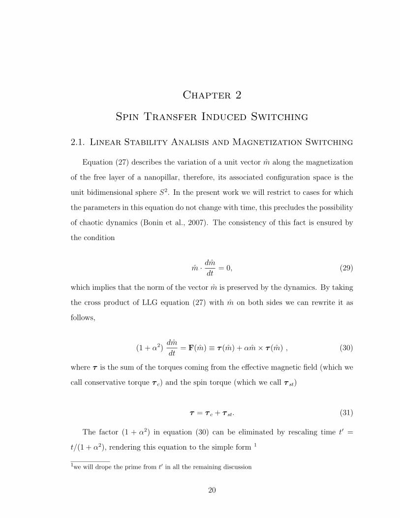
The fact that ε(m) is conserved 2 specifies uniquely the trajectory, which can

then be thought as the intersection of two surfaces, namely ε(m) = ε0 and m2 = 1.

These orbits describe the precession of m around the local effective magnetic field

(for an illustration see Figure 2.1). When damping is introduced the energy reduces

with time and the magnetization spirals down to directions which minize it. Energy

minima are therefore the only stable stationary solutions for the LLG equation under

this condition. This situation can be dramatically altered with the introduction of

spin torque which is able to stabilize equilibria otherwise corresponding to energy

maxima and also precession cycles may become stable dynamical attractors (Bonin

et al., 2007).

Even though exact dynamical solutions for equation (32) may be found for non-

trivial but highly symmetric energy functions (see e.g. Sukhov and Berakdar (2009)),

2This is a direct consequence of ∂ε∂m

· dmdt

= 0

21

a

p

Figure 2.1. Schematics of constant energy trajectories for a typicalnanopillar in the absence of external magnetic field

it is generally a difficult task and that degree of detail is seldom necessary. For mem-

ory applications mainly the knowledge of stable stationary magnetic configurations

is needed 3 and this can be gained by linear stability analysis. Linear stability anal-

ysis usually proceeds by finding the equilibrium orientations, m0, as functions of the

controllable parameters, which in typical experiments are the external magnetic field,

ωH , and the current, ωI , these equilibria correspond to the zeroes of F

m0(ωI , ωH) : F(m0) = 0. (35)

Equation (32) is then linearized around a given equilibria to find its local stability

behavior. To do so it is convenient to choose a particular system of coordinates 4. In

spherical coordinates (φ, θ), the components of equation (32) along the unit vectors

eφ, eθ read as

φ sin θ = F φ(φ, θ), θ = F θ(φ, θ), (36)

3Stable oscillatory solutions are important for other kinds of applications such as nanoscale mi-crowave voltage generators, but we will not consider those dynamical regimes in the present work.

4This can be done also in a coordinate free language by introducing the tensor of covariant derivatives.

22

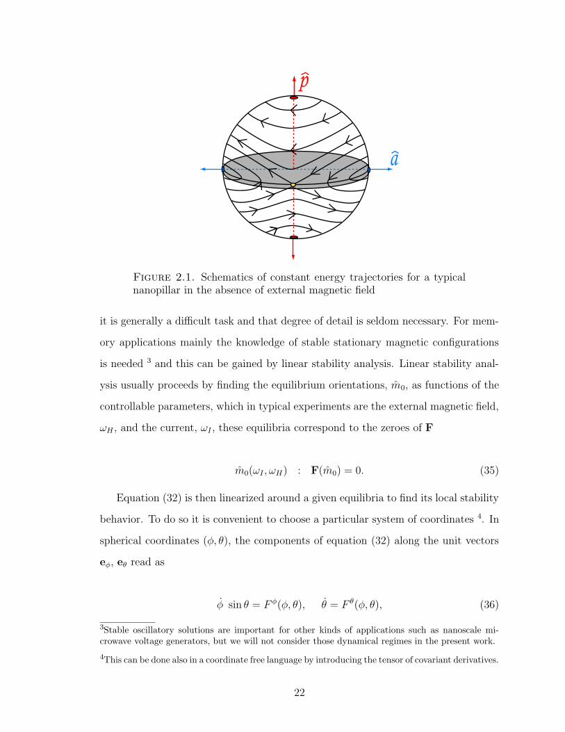
Table 2.1. Equilibria classification for the LLG equation

TrD < 0 TrD > 0

det D > 0

det D < 0

the linearized LLG equation can then be written in matrix form as 5

˙δφ

δθ

=

1sin θ

∂F φ

∂φ1

sin θ∂F φ

∂θ

∂F θ

∂φ∂F θ

∂θ

(φ0,θ0)

δφ

δθ

= D

δφ

δθ

, (37)

where δφ ≡ φ − φ0, δθ ≡ θ − θ0 are infinitesimal deviations from the equilibria

coordinates (φ0, θ0). The stability matrix D contains the information about the local

dynamical behavior surrounding a given equilibrium. In particular the eigenvalues of

this matrix given by

λ1,2 =TrD ±

√

(TrD)2 − 4 det D

2, (38)

determine the stability nature. If the real part of both λ1,2 is negative the equilibrium

would be stable and if the real part of any of them is positive it would be unstable.

From equation (38) this condition may be translated in terms of TrD and det D. For

an equilibrium to be stable the requirements are

TrD(neq) < 0, det D(neq) > 0. (39)

In fact the equilibria may be classified into stable and unstable centers and saddles

(always unstable) as shown in Table 2.1. From a mathematical standpoint the task is

then clear: find the position of an equilibrium as function of the parameters (ωH , ωI)

from equation (35), in particular infer the existence region of the equilibrium in the

5We are assuming the equilibrium of interest not to lie on a singular point of the spherical coordinates,that is the north or south poles, in such case we may circumvent the problem by simply choosinganother system of coordinates well defined at those points.

23

parameter space, evaluate then TrD and det D in this region and delimit the sub-

region for which conditions (39) are satisfied, this is the region at which the given

equilibrium is stable. At the boundaries of this region the stability disappear and the

given magnetic configuration then switches to another stable configuration 6, for some

illustrative examples of this analysis see Bazaliy et al. (2004); Morise and Nakamura

(2005).

Of particular interest is the value of the critical current at this boundary for a

fixed magnetic field ωIc(ωH), this is the so called switching current and gives the

critical current required to switch the magnetization of the nanopillar by means of

spin transfer torques. Reducing this current without reducing the intrinsic magnetic

stability of a given equilibrium 7 is one of the central challenges of the current memory

oriented research in spintronics. Understanding the efficiency of spin transfer torque

to produce switching constitutes then an important asset in this endeavour. The

following section elaborates further on this idea of the efficiency of spin transfer to

produce current induced switching, proposing a quantity that measures the ability of

spin torque to produce this switching.

6In the case for which no stable equilibrium exists in some region of the parameter space necessarilystable precession cycles must exist.

7A physical device able to represent a classical bit of information must have at least two equilibriumconfigurations with a degree of stability as to support thermal fluctuations (so that memory is kept)that can be switched between this two in a controllable manner (so that the writing process isreliable).

24

2.2. Invariant Form of Spin Transfer Switching Condition

Further insight about the stability conditions (39) and current induced switching

can be gained by analyzing them in terms of differential geometric quantities. In

particular consider the divergence of the field F(m) in the sphere, which in spherical

coordinates explicitly reads as

∇ · F =1

sin θ

(

∂

∂θ(sin θF θ) +

∂F φ

∂φ

)

, (40)

where ∇ is the gradient operator in the bidimensional unit sphere. From the form

of the stability matrix D in equation (37) it is easy to verify that at any equilibrium

point the following equality holds

∇ · F = TrD, (41)

even though ∇ · F and TrD are in general different functions.

Therefore ∇·F can replace TrD in the first inequality in (39). The ∇·F < 0 sta-

bility condition gets then a straightforward geometric interpretation when expressed

in integral form by means of Gauss theorem. Consider an arbitrary small closed con-

tour Γ in the unit sphere surrounding a given equilibrium, the line integral of the

normal component of F normal to the contour is related to the area integral of ∇ ·F

in the region inside the contour, A, as follows (Arfken, 1995)

∮

Γ

F · e⊥ dl =

∫

A

∇ · F dA, (42)

where e⊥ is the unit vector outward normal to Γ, and A is the area inside the contour.

Therefore TrD < 0, can be expressed as the condition that the average component of

F normal to any small contour around an equilibria is negative 8

8This condition rests in the assumption of a continuous variation of divF in the vicinity of the givenequilibria.

25

〈F · e⊥〉Γ < 0, (43)

in other words this condition is simply the requirement for the torque F to push

inwards in average at the vicinity of a stable equilibrium.

Let us now find ∇ · F using the explicit form of F. From equation (30) we find

∇ · F = ∇ · τ − α∇× τ , (44)

where ∇× τ is a pseudoscalar quantity 9 given by

∇× τ ≡ − 1

sin θ

[

∂τθ

∂φ− ∂

∂θ(sin θτφ)

]

. (45)

Equation (44) suggests that a Helmholtz decomposition of the vector field τ is de-

sirable. In such decomposition the divergenceless component of τ would be the one

that affects ∇·F from pure damping origin whereas the irrotational component would

appear as a direct modification of ∇·F. Fortunately the conservative torque, τ c, and

spin transfer torque, τ st, are already a natural Helmholtz decomposition of τ (see

eq. (31)) 10

τ c = −∇ε(m)×m, ∇ · τ c = 0

τ st = ωI g(m) [m×(s × m)], ∇× τ st = 0,

(46)

with above equations we can then write equation (44) in the following way

∇ · F = ∇ · τ st − α∇× τ c = ∇ · τ st − α∇2ε. (47)

9The curl “∇×” in a bidimensional space has a scalar character.

10That τ c is divergenceless is a direct consequence of it being conservative, the condition of τ st

being irrotational is, nevertheless, not so natural and in fact related to the particular form of τ st

in metallic nanopillars, indeed for other structures like magnetic tunnel junctions there is an non-irrotational component of the spin torque known as perpendicular spin torque, for a review on spintransfer torques in magnetic tunnel junctions see Sun and Ralph (2008).

26

Equation (47) contains important insights into the identification of a quantity

that represents the ability of spin transfer torque to poduce magnetic switching, in

the sense that we have explicitly separated out the quantity that determines wether

an equilibrium is stable or not, that is ∇ ·F, into a contribution that comes from the

intrinsic free magnetic dynamics of the system, namely −α∇2ε, plus a contribution

that depends only on the spin torque, that is ∇ · τ st.

To understand the limits on which ∇ · τ st plays the role of switching efficiency of

spin torque, and to further ellaborate into what this concept means, let us examine

more carefully how the magnetic switching in nanopillars occurs. If we go back

to Table 2.1 we can see that an originally stable magnetic configuration can be made

unstable, and therefore produce switching, by either changing the sign of TrD (which

is equal to ∇·F at the equilibrium) or the sign of det D. As mentioned in section 1.2

the dimensionless damping parameter is typically smaller than 1 (α ∼ 0.01), and

therefore constitutes a naturally small parameter of the system. It can be proved 11

that the sign of the determinant, and therefore the critical current at which it becomes

zero, is independent of α. On the contrary ∇ · F, and thus the critical current at

which it becomes zero, explicitly depends on α. Moreover ∇2ε would be of the order

of the magnetic constants defined in equation (28) for any equilibrium, therefore

equation (47) implies that the critical current at which ∇ ·F becomes zero, ωIc, is in

general small as compared to the magnetic constants

ωIc

ω∼ α. (48)

where ω designates generically the magnetic constants. On the contrary the critical

current associated with det D = 0 would generally be of the order of the magnetic

constants 12. Because of this situation, switching will be, for most cases, achieved by

11see section 2.3.

12A concrete illustration of this considerations will be given in section 3.1

27

changing the sign of ∇ · F rather than that of det D 13, in this sense the tendency

of spin torque to stabilize or destabilize a given equilibrium can be associated with

the tendency of it to make ∇ · F negative or positive and in particular the critical

current, ωIc, would be that for which ∇ · F∣

∣ωIc = 0.

Strictly speaking, spin torque affects ∇ · F not only directly via ∇ · τ st but it

also indirectly modifies the term −α∇2ε(m) in equation (47), because it changes the

position of the equilibrium, m, as a function of the current. Nevertheless because the

critical currents are of first order in α (equation (48)), the shifting of the equilibrium

points induced by spin torque would be of first order in α as well

meq(ωIc) = meq(0) + ∆meq, ∆meq ∝ ωIc ∝ α, (49)

therefore the contribution to ∇ · F coming from the equilibrium shifting induced by

spin torque is of order α2, and can reasonably be neglected. In this regime it is

therefore legitimate to associate the spin torque induced modification of ∇ · F with

∇ · τ st, and this quantity can be confidently identified with spin torque switching

ability. Moreover a simplified version of the stability condition can be written,

∇ · τ st

∣

∣

m(0)≤ α∇2ε

∣

∣

m(0)+ O(α2), (50)

where m(0) is the zero current orientation of the equilibrium in consideration, with

equality achieved at the critical switching current. Importantly, all quantities in (50)

are evaluated at the unperturbed equilibrium point m(0). In comparison, using ex-

pression (39) one needs to perform an explicit calculation of meq(ωIc) even in the first

order expansion in α (see e.g. Bazaliy et al. (2004); Sodemann and Bazaliy (2009)).

This welcome simplification is possible because ∇ ·F and TrD are different functions

coinciding only at equilibrium points, and ∇ · F proves to be a more convenient dis-

criminator. Additional simplification is provided by the fact that the left hand side

13This situation is not absolutely precluded and will be one of the central issues considered insection 2.3.

28

P=0.6

P=0.4

P=0.2

3π/4π/2π/40

stτωI

ϑ

π

0

0.5

1

1.5

2

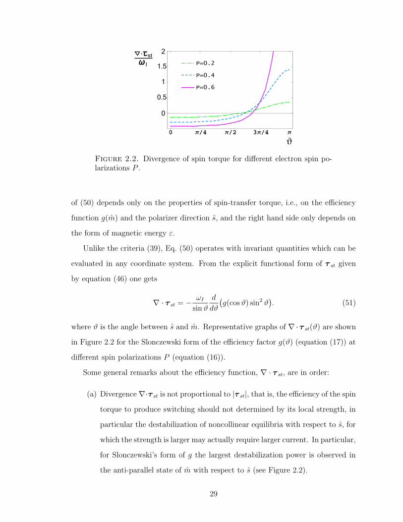
Figure 2.2. Divergence of spin torque for different electron spin po-larizations P .

of (50) depends only on the properties of spin-transfer torque, i.e., on the efficiency

function g(m) and the polarizer direction s, and the right hand side only depends on

the form of magnetic energy ε.

Unlike the criteria (39), Eq. (50) operates with invariant quantities which can be

evaluated in any coordinate system. From the explicit functional form of τ st given

by equation (46) one gets

∇ · τ st = − ωI

sin ϑ

d

dϑ

(

g(cos ϑ) sin2 ϑ)

. (51)

where ϑ is the angle between s and m. Representative graphs of ∇· τ st(ϑ) are shown

in Figure 2.2 for the Slonczewski form of the efficiency factor g(ϑ) (equation (17)) at

different spin polarizations P (equation (16)).

Some general remarks about the efficiency function, ∇ · τ st, are in order:

(a) Divergence ∇·τ st is not proportional to |τ st|, that is, the efficiency of the spin

torque to produce switching should not determined by its local strength, in

particular the destabilization of noncollinear equilibria with respect to s, for

which the strength is larger may actually require larger current. In particular,

for Slonczewski’s form of g the largest destabilization power is observed in

the anti-parallel state of m with respect to s (see Figure 2.2).

29

0.25 0.5 0.75 1 Pπ/2

3π/4

πϑ∗

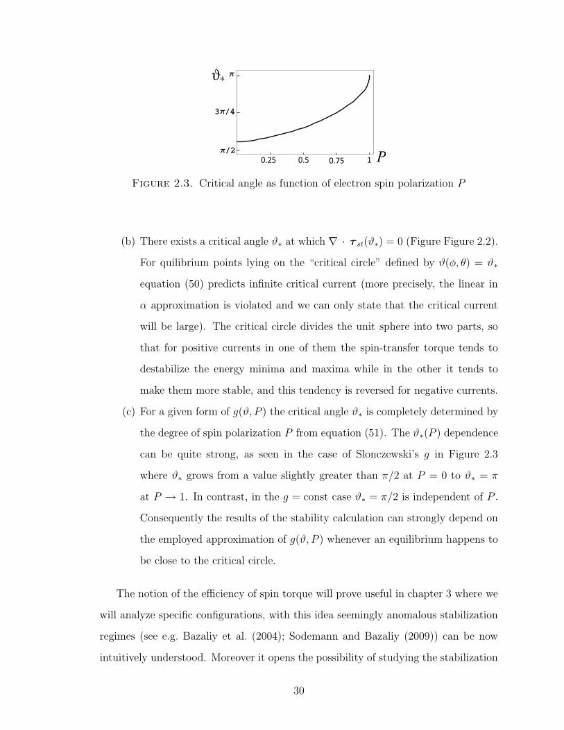
Figure 2.3. Critical angle as function of electron spin polarization P

(b) There exists a critical angle ϑ∗ at which ∇ · τ st(ϑ∗) = 0 (Figure Figure 2.2).

For quilibrium points lying on the “critical circle” defined by ϑ(φ, θ) = ϑ∗

equation (50) predicts infinite critical current (more precisely, the linear in

α approximation is violated and we can only state that the critical current

will be large). The critical circle divides the unit sphere into two parts, so

that for positive currents in one of them the spin-transfer torque tends to

destabilize the energy minima and maxima while in the other it tends to

make them more stable, and this tendency is reversed for negative currents.

(c) For a given form of g(ϑ, P ) the critical angle ϑ∗ is completely determined by

the degree of spin polarization P from equation (51). The ϑ∗(P ) dependence

can be quite strong, as seen in the case of Slonczewski’s g in Figure 2.3

where ϑ∗ grows from a value slightly greater than π/2 at P = 0 to ϑ∗ = π

at P → 1. In contrast, in the g = const case ϑ∗ = π/2 is independent of P .

Consequently the results of the stability calculation can strongly depend on

the employed approximation of g(ϑ, P ) whenever an equilibrium happens to

be close to the critical circle.

The notion of the efficiency of spin torque will prove useful in chapter 3 where we

will analyze specific configurations, with this idea seemingly anomalous stabilization

regimes (see e.g. Bazaliy et al. (2004); Sodemann and Bazaliy (2009)) can be now

intuitively understood. Moreover it opens the possibility of studying the stabilization

30

ability of non-standard functional forms of the spin torque like those recently proposed

for antiferromagnetic nanopillars (Haney et al., 2008).

It is important to recognize that the low current assumption is necessary for ∇·τ st

to meaningfully represent the switching ability, fortunately, this is the case for the

typical critical currents. This switching is, nevertheless not fast, in the sense that it

generally requires several precessional turns, each one typically of the order 100ps,

and during all this time the current is kept at the same constant value. Another

approach is the so-called “ultrafast switching”, in which high current pulses are ap-

plied in durations shorter than the typical precessional turns (Garzon et al., 2008),

in this regime the local strength of the spin torque is understood to be the important

quantity determining switching, rather than the divergence proposed in the present

work. Even though it has been generally shown that the total energy required for

switching is generally lower in the ultrafast regime, to produce the fast pulses in sim-

ple manners that could eventually be conveniently incorporated into memory devices

remains challenging. Both approaches are therefore still significant candidates to be

the switching mechanism in an eventually practical magnetic bit element.

31

2.3. Saddle Point Stabilization and Transcritical Bifurca-

tions

The results obtained in the previous section relied on the idea that the quantity

that determines switching in the limit of low damping was solely ∇ ·F = TrD, based

on the assumption that the sign of the determinant is independent of the damping

parameter α. In fact the following relation can be derived from equation (30)

det Dα = (1 + α2) det Dα=0 ≡ (1 + α2) det Dτ , (52)

which shows that α plays no role determining the change of sign in det D. Contrary

to ∇ · F, det D is not in general additive with respect to the addition of torques,

this property was crucial in separating the contributions of the conservative and spin

torques in ∇ ·F. Nevertheless the following decomposition rule can be written at an

equilibrium point in a special coordinate system where the polar angle ϑ is measured

with respect to the polarizer direction s 14

det Dτ = det Dτc + det Dτst −∂τϑ

c

∂ϑ

(

∂τϑst

∂ϑ− cos ϑ

sin ϑτϑst

)

(53)

where the matrices D appearing in above equation correspond to the same definition

given in equation (37) with the corresponding components of the specified vector field.

This equation is not very illuminating in general except for particular cases when the

last term vanishes and we can think of the determinant as being additive 15.

Since spin torque can stabilize and destabilize equilibria which at zero current cor-

respond to maxima and minima of energy by changing the sign of ∇ · F through its

direct modification of ∇ · τ st, then, natural questions that arise are: can the spin

14It is necessary that this equilibrium point is not any of the singular points of the coordinate system

15Those will be considered later in this section in the contex of transcritical bifurcations.

32

torque stabilize equilibria which are saddle points at zero current?, and can spin

torque destabilize energy minima or maxima by converting them into saddles 16?.

At first glance the problem may seem very similar to the one already solved in

the previous section, only that in this case we have to study when the function

det Dτ changes sign as the current is increased. Nevertheless, the fact that there is

no generally a small parameter involved is reflected in the fact that equilibria will

considerably shift their positions as the current is increased and therefore a proper

identification of an efficiency function associated with the ability of spin torque to

produce stabilization is in general not possible.

Other fundamental considerations make the problem of saddle point stabilization

substantially different from that of maxima and minima. In particular centers 17 and

saddles as zeroes of the vector field F differ in a characteristic topological property

called winding number or Poincare index. The Poincare index associated with a

saddle is −1 whereas for a center is 1. The Poincare index theorem for the two

dimensional sphere states that the sum of indices of all isolated fixed points equals 2.

This theorem can be expressed in the following formula

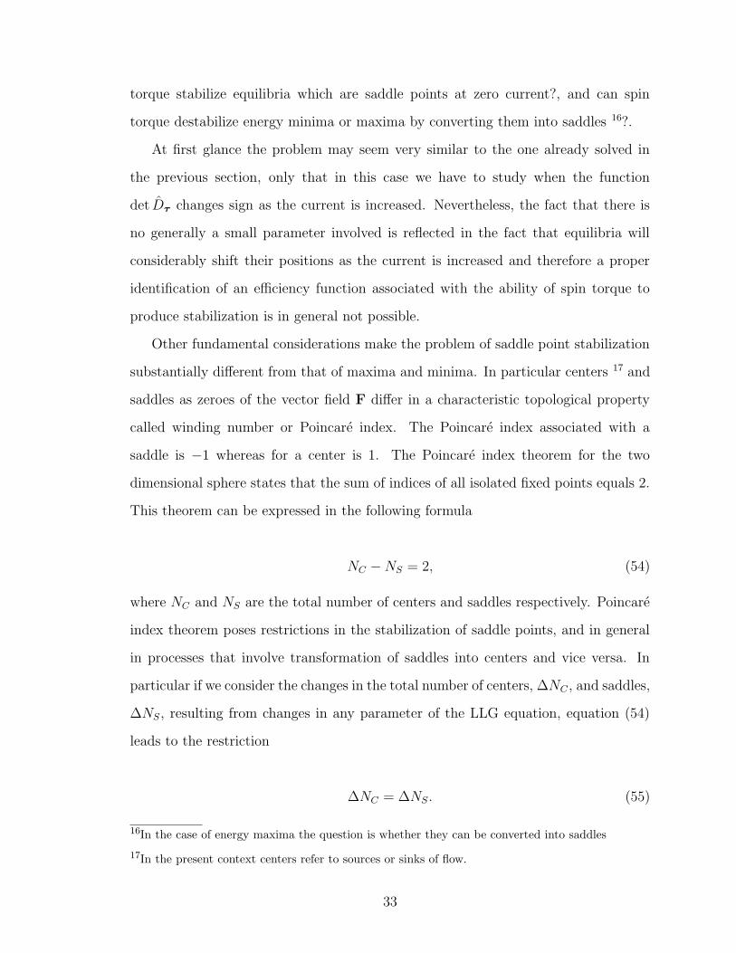
NC − NS = 2, (54)

where NC and NS are the total number of centers and saddles respectively. Poincare

index theorem poses restrictions in the stabilization of saddle points, and in general

in processes that involve transformation of saddles into centers and vice versa. In

particular if we consider the changes in the total number of centers, ∆NC , and saddles,

∆NS, resulting from changes in any parameter of the LLG equation, equation (54)

leads to the restriction

∆NC = ∆NS. (55)

16In the case of energy maxima the question is whether they can be converted into saddles

17In the present context centers refer to sources or sinks of flow.

33

This restriction in particular prohibits the possibility of locally transforming an iso-

lated saddle into an isolated center, that process would imply ∆NS = −1 and

∆NC = 1 in clear contradiction with this restriction 18. Therefore it is necessary

for an isolated saddle to become a center that other “distant” fixed points exchange

their nature as well, and this is what we mean by non-local.

A possible scenario suggested by the restriction (55) is the saddle-center annihi-

lation. This process is the one in which as the current is increased a saddle and a

center approach each other merging at certain critical current and dissapearing as a

consequence, in this process both the number of saddles and centers is decreased by

1, and therefore the condition (55) is satisfied 19. It turns out that the saddle-center

annihilation is in fact the most generic scenario and this bifurcation is robust (Craw-

ford, 1991), in the sense that occurs for small pertubations in the configutarion of the

device.

On the other hand, the non-local exchange of stability nature of two or more equi-

libria can occur but require special symmetry conditions that restrict their possible

shiftings as the current is increased, these are normally discrete symmetries of the

total torque under special transformations such as reflections or rotations 20. This

type of bifurcation is not robust in the sense that it is replaced by a merging type

bifurcation when the configuration is slightly perturbed and the underlying symmetry

is broken.

From above considerations it is clear that the saddle point stabilization problem is

qualitatively different from that of centers (which correspond to energy minima and

maxima at zero currents). Moreover the problem in general requires careful study of

the shifting of equilibria as the current is increased, this makes it technically difficult,

18The reciprocal process is evidently prohibited as well.

19By the same argument the saddle-center creation is an allowed process as well, in such case thenumber of saddles an centers increases by 1.

20A particular illustration of these situations is given in section 3.2.

34

and unless simple forms of the spin torque and special symmetries are involved it is

analytically untractable.

A particularly interesting type of bifucartion existing under special conditions is

the transcritical bifurcation (Crawford, 1991). This appears in the case when the

polarizer s coincides with an equilibrium m0 which is a saddle point at zero current.

Therefore the spin torque is zero at this equilibrium and as the current increases the

equilibrium remains “pinned” along the direction of the polarizer. In this situation

we must consider equation equation (53) in the limit ϑ → 0 and the last term may

be shown to vanish, leading to

limϑ→0

det Dτ = det Dτc(ϑ = 0) + limϑ→0

det Dτst, (56)

where Dτc(ϑ = 0) is basically the determinant of the stability matrix at the saddle

point in the absence of spin torque which is necessarily negative (see Table 2.1), the

determinant of the stability matrix associated with spin torque can be proven to be

limϑ→0

det Dτst = (ωIg(ϑ = 0, P ))2. (57)

Therefore there is a critical current at which det Dτ = 0 and the saddle becomes a

center given by

ωIcrit =

√

− det Dτ c(ϑ = 0)

g(ϑ = 0, P ). (58)

According to the previous discussions of the Poincare index theorem this trans-

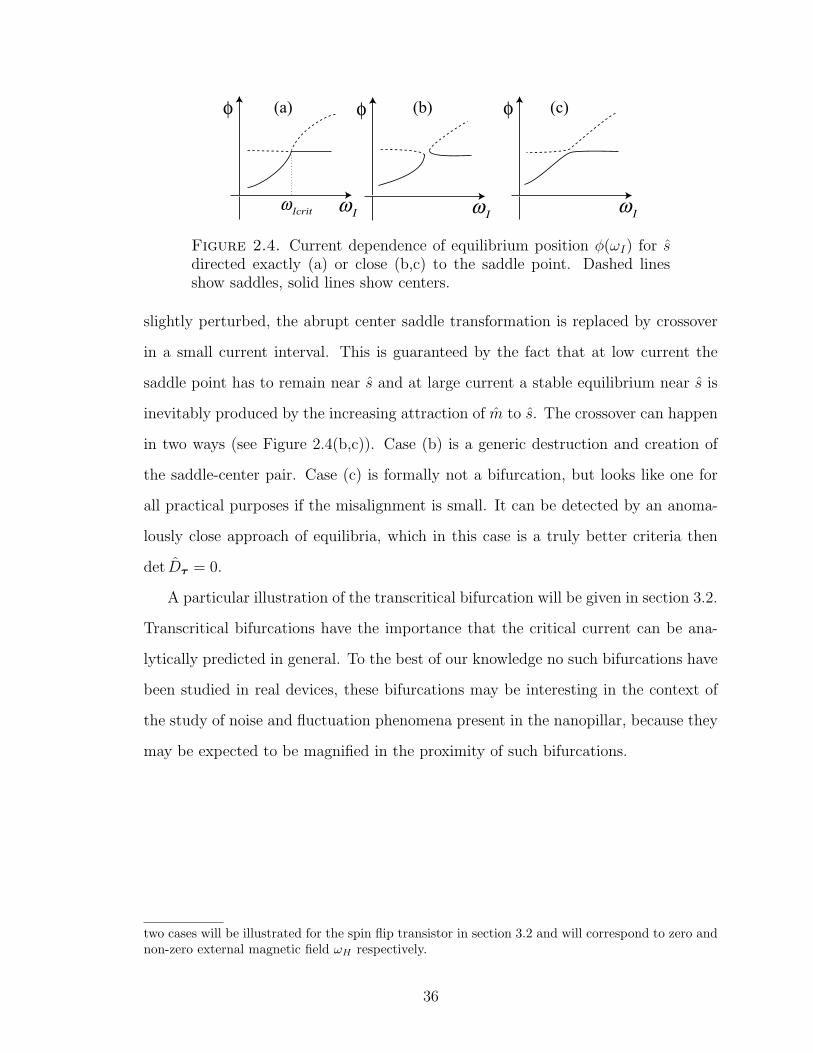
formation cannot occur for an isolated saddle point. In the generic case what occurs

is that a center approaches the saddle and at the critical current they “exchange”

their stability nature in a collision-like process (see Figure 2.4(a)), which is the tran-

scritical bifurcation itself (Crawford, 1991) 21. When the position of the polarizer is

21What “generic” means in the present context is that there are no special symmetries restrictingthe approach of the center to the direction of the polarizer as the current increases, another “non-genreric” scenario is that more than one center approach the saddle as the current increases, these

35

φ

I

φ φ(a) (c)(b)

ωI

ωI

ωIcritω

Figure 2.4. Current dependence of equilibrium position φ(ωI) for sdirected exactly (a) or close (b,c) to the saddle point. Dashed linesshow saddles, solid lines show centers.

slightly perturbed, the abrupt center saddle transformation is replaced by crossover

in a small current interval. This is guaranteed by the fact that at low current the

saddle point has to remain near s and at large current a stable equilibrium near s is

inevitably produced by the increasing attraction of m to s. The crossover can happen

in two ways (see Figure 2.4(b,c)). Case (b) is a generic destruction and creation of

the saddle-center pair. Case (c) is formally not a bifurcation, but looks like one for

all practical purposes if the misalignment is small. It can be detected by an anoma-

lously close approach of equilibria, which in this case is a truly better criteria then

det Dτ = 0.

A particular illustration of the transcritical bifurcation will be given in section 3.2.

Transcritical bifurcations have the importance that the critical current can be ana-

lytically predicted in general. To the best of our knowledge no such bifurcations have

been studied in real devices, these bifurcations may be interesting in the context of

the study of noise and fluctuation phenomena present in the nanopillar, because they

may be expected to be magnified in the proximity of such bifurcations.

two cases will be illustrated for the spin flip transistor in section 3.2 and will correspond to zero andnon-zero external magnetic field ωH respectively.

36

Chapter 3

Selected Applications

3.1. Metallic Nanopillar with In-plane Magnetic Field

The spin transfer switching in metallic nanopillars with an external in-plane mag-

netic field perpendicular to the direction of the easy axis has been extensively studied

both theoretically (see eg. Sun (2000); Smith et al. (2005); Sodemann and Bazaliy

(2009)) and experimentally (see eg. Mancoff et al. (2003); Smith et al. (2005); Garzon

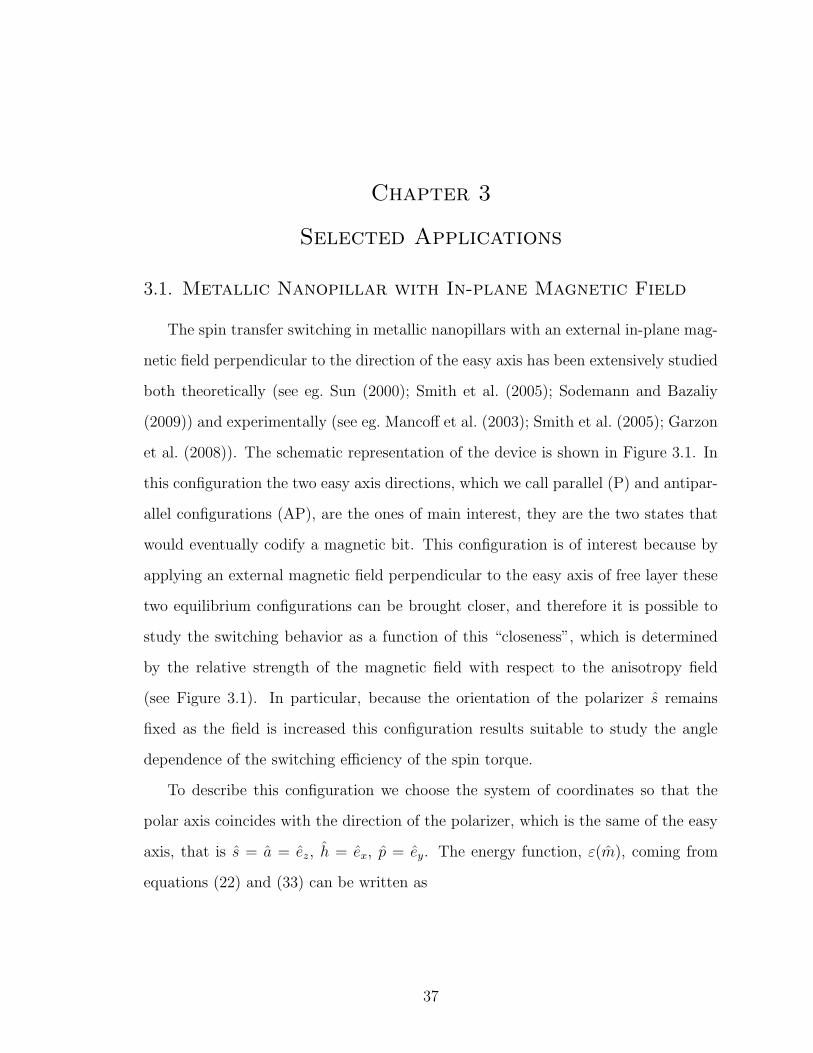
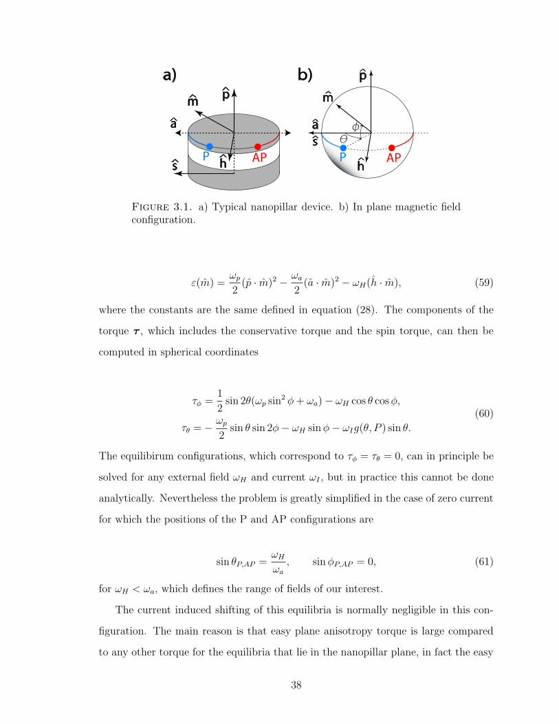
et al. (2008)). The schematic representation of the device is shown in Figure 3.1. In

this configuration the two easy axis directions, which we call parallel (P) and antipar-

allel configurations (AP), are the ones of main interest, they are the two states that

would eventually codify a magnetic bit. This configuration is of interest because by

applying an external magnetic field perpendicular to the easy axis of free layer these

two equilibrium configurations can be brought closer, and therefore it is possible to

study the switching behavior as a function of this “closeness”, which is determined

by the relative strength of the magnetic field with respect to the anisotropy field

(see Figure 3.1). In particular, because the orientation of the polarizer s remains

fixed as the field is increased this configuration results suitable to study the angle

dependence of the switching efficiency of the spin torque.

To describe this configuration we choose the system of coordinates so that the

polar axis coincides with the direction of the polarizer, which is the same of the easy

axis, that is s = a = ez, h = ex, p = ey. The energy function, ε(m), coming from

equations (22) and (33) can be written as

37

APP

>

>

>

>

p

hs

a

>

m

a) b)

P AP

a

p

h

s θφ

>>

>>

m

>

Figure 3.1. a) Typical nanopillar device. b) In plane magnetic fieldconfiguration.

ε(m) =ωp

2(p · m)2 − ωa

2(a · m)2 − ωH(h · m), (59)

where the constants are the same defined in equation (28). The components of the

torque τ , which includes the conservative torque and the spin torque, can then be

computed in spherical coordinates

τφ =1

2sin 2θ(ωp sin2 φ + ωa) − ωH cos θ cos φ,

τθ = − ωp

2sin θ sin 2φ − ωH sin φ − ωIg(θ, P ) sin θ.

(60)

The equilibirum configurations, which correspond to τφ = τθ = 0, can in principle be

solved for any external field ωH and current ωI , but in practice this cannot be done

analytically. Nevertheless the problem is greatly simplified in the case of zero current

for which the positions of the P and AP configurations are

sin θP,AP =ωH

ωa

, sin φP,AP = 0, (61)

for ωH < ωa, which defines the range of fields of our interest.

The current induced shifting of this equilibria is normally negligible in this con-

figuration. The main reason is that easy plane anisotropy torque is large compared

to any other torque for the equilibria that lie in the nanopillar plane, in fact the easy

38

axis anisotropies and the typical magnetic fields used for these devices are about ∼10-

50mT, on the other hand the easy plane anisotropy for very thin free layers (thickness

of about 5nm) are about ∼1-2T, this means that the easy plane anisotropy strength,

ωp, is about a hundred times larger than the easy axis anisotropy, ωa. When the

currents are turned on the spin torque will tend to shift equilibria out of the easy

plane in the azimuthal direction at first order, but this effect is greatly suppresed by

the strong easy plane anisotropy, as a consequence the first order spin torque induced

shifting, in powers of ωI/ωp is

sin θP,AP =ωH

ωa

+O(

ωI

ωp

)2

, sin φP,AP = −gP,APωI

ωp

(

1 +ωa

ωp

)

+O(

ωI

ωp

)2

. (62)

Where gP,AP = g(θP,AP , P ). Because the applied field ωH determines uniquely the

polar angle orientation of the equilibria, θ, we will use them interchangeably in the

rest of the discussion, therefore whenever θ appears in the rest of this section it must

be understood that it is the polar orientation of the equilibria which is fixed by the

external magnetic field. To determine the switching currents as a function of the

field we use the ideas developed in section 2.2, according to which the sign of the

divergence of the total torque, ∇ · F, determines whether an equilibrium is stable or

not. before that, in order to illustrate that the determinant does not play a major

role in determining the critical currents for switching between energy minima and

maxima, let us compute it explicitly. From the definition of the stability matrix D

from equation (37) we obtain

1

1 + α2detD = ωa(ωp + ωa) cos2 θ + O(ω2

I ). (63)

Therefore it is clear that it remains positive in the regime of our interest and does

not affect switching. On the other hand the divergence is

39

∇ · F = − ωI(g(θ) cos θ +d

dθ(g(θ, P ) sin θ))

− α(ωp cos 2φ + (ωp sin2 φ + ωa)(1 + cos2 θ)).

(64)

The first term is the divergence of spin torque, but in this case the angle between

the polarizer and the free layer polarization is simply the polar angle ϑ = θ (see

equation (51)). The second term is the curl of the conservative torque (compare with

equation (47)). The condition of stability is reduced to the negativity of ∇ · F. To

show how the divergence of spin torque can be used to quantify its switching ability

let us contrast the stability behavior for two functional forms of the efficiency factor

g(θ, P ), namely the g = const approximation and the Slonczewski form for g (see

equation (17)).

For the g constant approximation the currents for which the P and the AP configu-

rations are stable are given by

ωI ≷ ∓αωp + ωa(2 − (ωH/ωa)

2)

2g√

1 − (ωH/ωa)2(65)

where >, − (<, +) corresponds to the P (AP) stability region (See figure Figure 3.2d),

with equality achieved at the critical switching current. The switching current is

symmetric for switching from P to AP and AP to P (only difers by sign), and exhibits

the 1/ cos θ divergence reported in previous studies (Sun, 2000; Mancoff et al., 2003).

For the Slonczewski g factor, the stability condition for P reads as,

ωI > −αωp + ωa(2 − (ωH/ωa)

2)

2gN

√

1 − (ωH/ωa)2 + g2Nf(ωH/ωa)2

, (66)

with equality achieved at the critical switching current. For the AP equilibrium we

have

ωI ≶ αωp + ωa(2 − (ωH/ωa)

2)

2gS

√

1 − (ωH/ωa)2 − g2Sf(ωH/ωa)2

, (67)

40

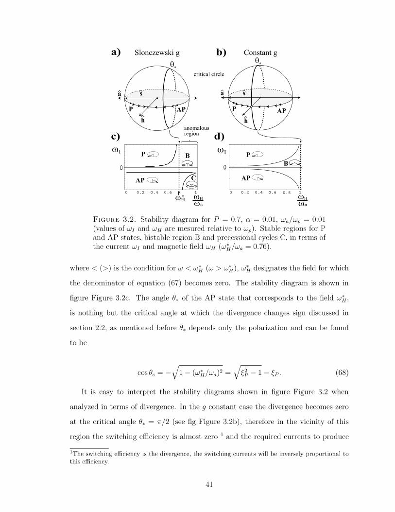
s

critical circle

Slonczewski g Constant g

0 0.2 0.4 0.6 1

0

anomalous

region

0

0 0.2 0.4 0.6 0.8 1

*

a

> >

a

>

s

>

h

>

h

>

P AP APP

P

AP

B

C

B

P

AP

a) b)

c) d)

ωI ωI

ωHωHωa

ωH

ωa

θ*

θ*

Figure 3.2. Stability diagram for P = 0.7, α = 0.01, ωa/ωp = 0.01(values of ωI and ωH are mesured relative to ωp). Stable regions for Pand AP states, bistable region B and precessional cycles C, in terms ofthe current ωI and magnetic field ωH (ω∗

H/ωa = 0.76).

where < (>) is the condition for ω < ω∗H (ω > ω∗

H), ω∗H designates the field for which

the denominator of equation (67) becomes zero. The stability diagram is shown in

figure Figure 3.2c. The angle θ∗ of the AP state that corresponds to the field ω∗H ,

is nothing but the critical angle at which the divergence changes sign discussed in

section 2.2, as mentioned before θ∗ depends only the polarization and can be found

to be

cos θc = −√

1 − (ω∗H/ωa)2 =

√

ξ2P − 1 − ξP . (68)

It is easy to interpret the stability diagrams shown in figure Figure 3.2 when

analyzed in terms of divergence. In the g constant case the divergence becomes zero

at the critical angle θ∗ = π/2 (see fig Figure 3.2b), therefore in the vicinity of this

region the switching efficiency is almost zero 1 and the required currents to produce

1The switching efficiency is the divergence, the switching currents will be inversely proportional tothis efficiency.

41

switching diverge in the linear approximation, on the contrary for zero magnetic field

ωH = 0, that is for θ = 0, π, the divergence is maximum and then the critical

current is minimum. The symmetry of the switching diagram is naturally explained

from the symmetry of the magnitude of the divergence about θ = π/2.

For the slonczewski g factor we have the same qualitative behavior for ωH < ω∗H ,

except for the high asymmetry of the switching current, which is smaller for switch-

ing from AP to P than from P to AP at low magnetic fields, this comes from the

high asymmetry of the divergence around θ = π/2 as shown in Figure 2.2. As ωH

approaches ω∗H the AP state approaches the critical angle θ∗ at which the diver-

gence vanishes and therefore the required switching current diverges. The seemingly

anomalous switching behavior for ωH > ω∗H , in which AP is stable for positive cur-

rents and unstable for sufficiently large negative currents, is explained by the fact

that the divergence has now the same sign that it has for the P configuration at a

given field, therefore both P and AP tend to be stabilized for positive currents and

destabilized for sufficiently large negative currents. An interesting region emerges in

this regime where neither of the equilibria is stable suggesting the existence of an

stable precession cycle (see Figure 3.2(c)).

Above discussion shows how the divergence of spin torque captures the essential

features of a quantity representing its switching ability.

42

3.2. Spin Flip Transistor

The previous discussion has been focused on the spin transfer in nanopillar geome-

tries, nevertheless some other devices can be analyzed within the same formalism of

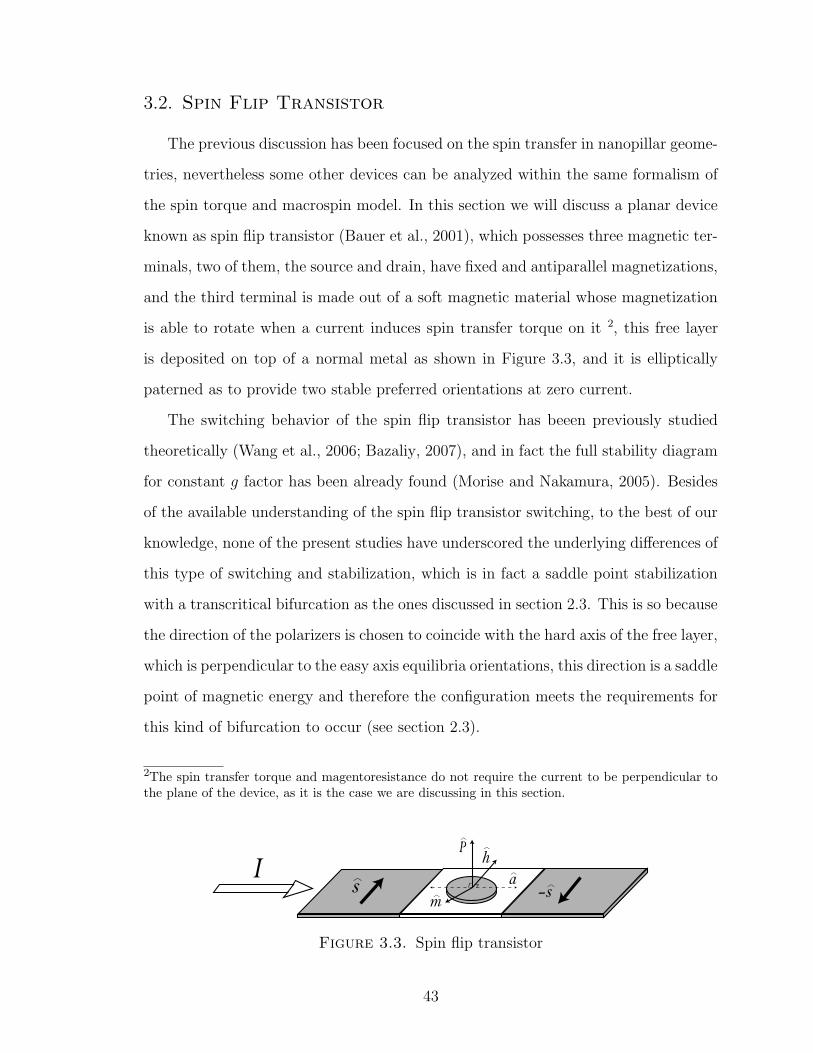
the spin torque and macrospin model. In this section we will discuss a planar device

known as spin flip transistor (Bauer et al., 2001), which possesses three magnetic ter-

minals, two of them, the source and drain, have fixed and antiparallel magnetizations,

and the third terminal is made out of a soft magnetic material whose magnetization

is able to rotate when a current induces spin transfer torque on it 2, this free layer

is deposited on top of a normal metal as shown in Figure 3.3, and it is elliptically

paterned as to provide two stable preferred orientations at zero current.

The switching behavior of the spin flip transistor has beeen previously studied

theoretically (Wang et al., 2006; Bazaliy, 2007), and in fact the full stability diagram

for constant g factor has been already found (Morise and Nakamura, 2005). Besides

of the available understanding of the spin flip transistor switching, to the best of our

knowledge, none of the present studies have underscored the underlying differences of

this type of switching and stabilization, which is in fact a saddle point stabilization

with a transcritical bifurcation as the ones discussed in section 2.3. This is so because

the direction of the polarizers is chosen to coincide with the hard axis of the free layer,

which is perpendicular to the easy axis equilibria orientations, this direction is a saddle

point of magnetic energy and therefore the configuration meets the requirements for

this kind of bifurcation to occur (see section 2.3).

2The spin transfer torque and magentoresistance do not require the current to be perpendicular tothe plane of the device, as it is the case we are discussing in this section.

Is

>

-s

>

m

>

a

>

h

>P

>

Figure 3.3. Spin flip transistor

43

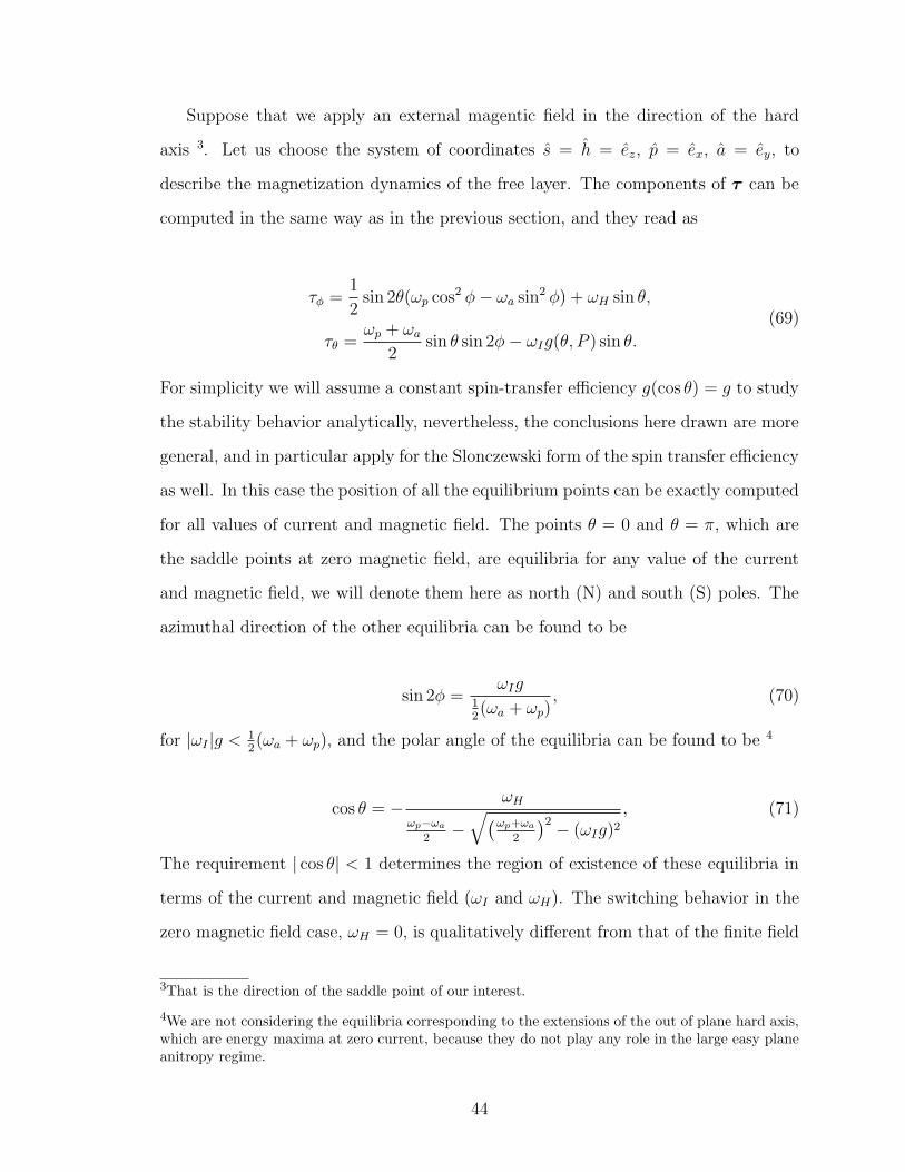
Suppose that we apply an external magentic field in the direction of the hard

axis 3. Let us choose the system of coordinates s = h = ez, p = ex, a = ey, to

describe the magnetization dynamics of the free layer. The components of τ can be

computed in the same way as in the previous section, and they read as

τφ =1

2sin 2θ(ωp cos2 φ − ωa sin2 φ) + ωH sin θ,

τθ =ωp + ωa

2sin θ sin 2φ − ωIg(θ, P ) sin θ.

(69)

For simplicity we will assume a constant spin-transfer efficiency g(cos θ) = g to study

the stability behavior analytically, nevertheless, the conclusions here drawn are more

general, and in particular apply for the Slonczewski form of the spin transfer efficiency

as well. In this case the position of all the equilibrium points can be exactly computed

for all values of current and magnetic field. The points θ = 0 and θ = π, which are

the saddle points at zero magnetic field, are equilibria for any value of the current

and magnetic field, we will denote them here as north (N) and south (S) poles. The

azimuthal direction of the other equilibria can be found to be

sin 2φ =ωIg

12(ωa + ωp)

, (70)

for |ωI |g < 12(ωa + ωp), and the polar angle of the equilibria can be found to be 4

cos θ = − ωH

ωp−ωa

2−

√

(ωp+ωa

2

)2 − (ωIg)2

, (71)

The requirement | cos θ| < 1 determines the region of existence of these equilibria in

terms of the current and magnetic field (ωI and ωH). The switching behavior in the

zero magnetic field case, ωH = 0, is qualitatively different from that of the finite field

3That is the direction of the saddle point of our interest.

4We are not considering the equilibria corresponding to the extensions of the out of plane hard axis,which are energy maxima at zero current, because they do not play any role in the large easy planeanitropy regime.

44

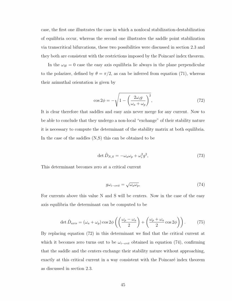
case, the first one illustrates the case in which a nonlocal stabilization-destabilization

of equilibria occur, whereas the second one illustrates the saddle point stabilization

via transcritical bifurcations, these two possibilities were discussed in section 2.3 and

they both are consistent with the restrictions imposed by the Poincare index theorem.

In the ωH = 0 case the easy axis equilibria lie always in the plane perpendicular

to the polarizer, defined by θ = π/2, as can be inferred from equation (71), whereas

their azimuthal orientation is given by

cos 2φ = −

√

1 −(

2ωig

ωa + ωp

)2

, (72)

It is clear therefore that saddles and easy axis never merge for any current. Now to

be able to conclude that they undergo a non-local “exchange” of their stability nature

it is necessary to compute the determinant of the stability matrix at both equilibria.

In the case of the saddles (N,S) this can be obtained to be

det DN,S = −ωaωp + ω2i g

2, (73)

This determinant becomes zero at a critical current

gωi−crit =√

ωaωp, (74)

For currents above this value N and S will be centers. Now in the case of the easy

axis equilibria the determinant can be computed to be

det Daxis = (ωa + ωp) cos 2φ

((

ωp − ωa

2

)

+

(

ωp + ωa

2cos 2φ

))

. (75)

By replacing equation (72) in this determinant we find that the critical current at

which it becomes zero turns out to be ωi−crit obtained in equation (74), confirming

that the saddle and the centers exchange their stability nature without approaching,

exactly at this critical current in a way consistent with the Poincare index theorem

as discussed in section 2.3.

45

This nonlocal type of stabilization is nevertheless not robust, and the underlying

reason for its existence is the inversion symmetry of the torque with respect to the

plane perpendicular to s. If this symmetry is slightly broken this abrupt exchange of

local stability behavior is replaced by a merging. This is the case when a magnetic

field pointing along s is introduced. In this case the position of the easy axis directions

is given by equations (70) and (71). In particular from equation (71) we can see that

as the current is increased the easy axis equilibria start approaching the saddle 5 and

they merge with it for cos θ = ±1, thus the current and the field are related by

ωH = ±

√

(

ωa + ωp

2

)2

− (ωIg)2 − ωp − ωa

2

. (76)

where the + (−) corresponds to merging with the N (S) saddle. On the other hand

the determinant at the saddles (N and S) is given by

det D = −(

ωp + ωa

2

)2

+

((

ωp − ωa

2

)

± ωH

)2

+ ω2Ig

2, (77)

where the + (−) corresponds to the N (S) saddle. Thus the critical current for which

thes saddles become centers 6 is

ωIcritg =

√

(

ωp + ωa

2

)2

−((

ωp − ωa

2

)

± ωH

)2

, (78)

which is the same current at which the centers merge with saddle obtained from

equation (76).

This is a transcritical bifurcation with an extra special feature, namely the fact

that two equilibria “collide” with the saddle at the same time leaving only a center

afterwards. This feature of the bifurcation is not robust and emerges from another

underlying symmetry of the torque, in this case the rotation by π/2 around s which

is not broken by the introduction of a magentic field. When this symmetry is slightly

5For positive magnetic field they approach N (s) and for negative ones they approach S (−s).

6They both become centers at the same time

46

s

M1M2

L

M1M2

S

(a) (b)

(c) (e)(d)

a

>

a

>

h

>

h

>

s

>

Figure 3.4. Transcritical bifurcation in the spin flip transistor. (a)The dashed lines show how the positions of the easy axis equilibria(M1,2) approach the saddle, S, with increasing current and merge withit at a critical value given by eq. (78). (b) In-plane directions of s and

h that slightly break the π/2 rotation symmetry. The saddle mergeswith one of the centers, while the other one asymptotically approachess. (c-e) transformation of the field F during the merger of the saddlewith two centers in case (a).

broken the bifurcation is replaced by the “generic” case in which the saddle merges

with a single one of the approaching centers. Figure 3.4 sketches the situation of this

transcritical bifurcation, and how it is replaced when the symmetry is slightly broken.

47

Chapter 4

Summary and Conclusions

In the present work we have theoretically studied the stability properties of the

magnetization of a single domain ferromagnetic layer in the presence of an external

magnetic field, magnetic anisotropies and spin transfer torque.

By incorporating differential geometric quantities into the standard linear stability

analysis we have singled out a function that represents the ability of spin torque to

stabilize/destabilize equilibrium configurations corresponding to minima and maxima

of magnetic energy. This quantity is the divergence of spin torque, explicitly presented

in equation (51).

The meaning of this observation could be summarized in the following paragraph:

The free dynamics of the magnetization vector is divergenceless, that is, the effective

magnetic torques only produce precession around the energy minima and maxima;

when damping is introduced this behavior is modified, precession is then accompanied

by a spiraling motion into those orientations that minize the energy of the system,

this is a consequence of the damping torque having a finite divergence, which is nev-

ertheless small due to the smallness of the damping parameter α. When spin torque

is introduced the divergence map of the total torque can be dramatically modified,

due to the fact that spin torque is irrotational and therefore it only modifies the di-

vergenceful part of the total torque, that is the damping torque, which is otherwise

small due to the smallness of α. Consequently the local damping divergence can be

compensated and in some cases canceled by the divergence of spin torque, leading to

spin torque induced switching. This competition between damping and spin torque

is illustrated in equation (47).

48

This idea of divergence of spin torque as switching ability was applied in section 3.1

to the particular case of a bistable metallic nanopillar with an external in-plane mag-

netic field perpendicular to its easy axis. This allowed us, for example, to understand

the appearance of stability regions in the parameter space for the Slonczewski effi-

ciency factor g(θ; P ) (see equation (17)) which were absent in the g-constant stability

diagram as a consequence of the shifting of the angle for which the divergence vanishes

ϑ∗(P ) (see Figure 2.2 and Figure 2.3).

In general we expect the idea of divergence of spin torque as switching ability to

facilitate

• Understanding of some “unusual” switching regimes.

• Understanding of stability behavior for “non-trivial” spin torque functional

forms.

• Alternative device engineering to obtain maximum switching efficiency.

We have also addressed the question of stabilization of magnetization orientations

corresponding to saddle points. This stabilization requires a change in the sign of

the determinant of the stability matrix (see equation (37) and Table 2.1). Poincare

index theorem, nevertheless, constrains the stabilization process of a saddle point

requiring another equilibrium to be involved in the process. As a consequence, in the

generic case, saddles are not stabilized but simply merge with a center as the current

is increased 1.

However, under special conditions saddles can be stabilized by increasing the

current either in a process in which they exchange their stability nature with distant

equilibria or in a collision-like process with an approaching stable equilibrium. This

collision-like process is a transcritical bifurcation, and occurs whenever the direction

of the polarizer coincides with that of a saddle point of magnetic energy. The critical

bifurcation current can be analytically related to the determinant of the stability

matrix associated with the magnetic torque as shown in equation (58).

1Both equilibria will disappear for currents larger than the critical merging current

49

Finally, we have illustrated the saddle point stabilization problem in the spin flip

transistor, both when the saddles exchange their stability with distant equilibria (no

external magnetic field, ωH = 0) and when they merge with approaching centers

(finite external magnetic field, ωH 6= 0) as the current increases.

50

Bibliography

Arfken, G. B. (1995). Mathematical Methods for Physicists (Fourth ed.). San Diego,CA: Academic Press.

Ashcroft, N. and D. Mermin (1976). Solid State Physics. Thomson Learning.

Baibich, M. N., J. M. Broto, A. Fert, F. N. Van Dau, F. Petroff, P. Etienne,G. Creuzet, A. Friederich, and J. Chazelas (1988). Giant magnetoresistance of(001)fe/(001)cr magnetic superlattices. Physical Review Letters 61 (21), 2472–2475.

Bauer, G., Y. Nazarov, and A. Brataas (2001). Spin-flip transistor. Physica E-Low-

Dimensional Systems & Nanostructures 11 (2-3), 137–143.

Bazaliy, Y., B. Jones, and S. Zhang (1998). Modification of the Landau-Lifshitzequation in the presence of a spin-polarized current in colossal- and giant-magnetoresistive materials. Physical Review B 57 (6), R3213–R3216.

Bazaliy, Y., B. Jones, and S. Zhang (2004). Current-induced magnetization switchingin small domains of different anisotropies. Physical Review B 69 (9).

Bazaliy, Y. B. (2007). Magnetization dynamics in planar spin transfer devices andstabilization by repulsion in a spin-flip transistor. Applied Physics Letters 91 (26).

Berger, L. (1996). Emission of spin waves by a magnetic multilayer traversed by acurrent. Physical Review B 54 (13), 9353–9358.

Berkov, D. and J. Miltat (2008). Spin-torque driven magnetization dynamics: Micro-magnetic modeling. Journal of Magnetism and Magnetic Materials 320 (7), 1238– 1259.

Binasch, G., P. Grunberg, F. Saurenbach, and W. Zinn (1989). Enhanced mag-netoresistance in layered magnetic structures with antiferromagnetic interlayerexchange. Physical Review B 39 (7), 4828–4830.

Bonin, R., C. Serpico, G. Bertotti, I. D. Mayergoyz, and M. d’Aquino (2007). Analyt-ical study of magnetization dynamics driven by spin-polarized currents. European

Physical Journal B 59 (4), 435–445.

51

Brataas, A., G. Bauer, and P. Kelly (2006). Non-collinear magnetoelectronics. Physics

Reports-Review Section of Physics Letters 427 (4), 157–255.

Bruno, P. and C. Chappert (1991). Oscillatory coupling between ferromagnetic layersseparated by a nonmagnetic metal spacer. Physical Review Letters 67 (12), 1602–1605.

Crawford, J. (1991). Introduction to Bifurcation-Theory. Reviews of Modern

Physics 63 (4), 991–1037.

Garzon, S., L. Ye, R. A. Webb, T. M. Crawford, M. Covington, and S. Kaka (2008).Coherent control of nanomagnet dynamics via ultrafast spin torque pulses. Phys-

ical Review B 78 (18), 180401.

Haney, P. M., R. A. Duine, A. S. Nunez, and A. H. MacDonald (2008). Current-induced torques in magnetic metals: Beyond spin-transfer. Journal of Magnetism

and Magnetic Materials 320 (7), 1300–1311.

Krivorotov, I. N., N. C. Emley, J. C. Sankey, S. I. Kiselev, D. C. Ralph, and R. A.Buhrman (2005). Time-Domain Measurements of Nanomagnet Dynamics Drivenby Spin-Transfer Torques. Science 307 (5707), 228–231.

Landau, L. D. and E. M. Lifshitz (1984). L. D. Landau and E. M. Lifshitz Course on

Theoretical Physics, Volume 8: Electrodynamics of Continuous Media (Seconded.). Pergamon.

Lifshitz, E. M. and L. P. Pitaevskii (1981). L. D. Landau and E. M. Lifshitz Course

on Theoretical Physics, Volume 9: Statistical Physics, Part 2: Theory of the

Condensate State. Pergamon.

Mancoff, F., R. Dave, N. Rizzo, T. Eschrich, B. Engel, and S. Tehrani (2003). Angu-lar dependence of spin-transfer switching in a magnetic nanostructure. Applied

Physics Letters 83 (8), 1596–1598.

Morise, H. and S. Nakamura (2005). Stable magnetization states under a spin-polarized current and a magnetic field. Physical Review B 71 (1).

Myers, E., D. Ralph, J. Katine, R. Louie, and R. Buhrman (1999). Current-inducedswitching of domains in magnetic multilayer devices. Science 285 (5429), 867–870.

Parkin, S. P. (2004). Shiftable magnetic shift register and method of using the same.United States Patent (6,834,005).

Parkin, S. S. P., M. Hayashi, and L. Thomas (2008). Magnetic domain-wall racetrackmemory. Science 320 (5873), 190–194.

52

Parkin, S. S. P., N. More, and K. P. Roche (1990). Oscillations in exchange cou-pling and magnetoresistance in metallic superlattice structures: Co/ru, co/cr,and fe/cr. Physical Review Letters 64 (19), 2304–2307.

Ralph, D. C. and M. D. Stiles (2008). Spin transfer torques. Journal of Magnetism

and Magnetic Materials 320 (7), 1190–1216.

Slonczewski, J. C. (1996). Current-driven excitation of magnetic multilayers. Journal

of Magnetism and Magnetic Materials 159 (1-2), L1 – L7.

Smith, N., J. Katine, J. Childress, and M. Carey (2005). Angular dependence ofspin torque critical currents for CPP-GMR read heads. IEEE Transactions on

Magnetics 41 (10), 2935–2940.

Sodemann, I. and Y. Bazaliy (2009). Anomalous stabilization in a spin-transfer systemat high spin polarization. Journal of Applied Physics 105 (7), 07D114.

Stiles, M. and A. Zangwill (2002). Anatomy of spin-transfer torque. Physical Review

B 66 (1).

Sukhov, A. and J. Berakdar (2009). Local Control of Ultrafast Dynamics of MagneticNanoparticles. Physical Review Letters 102 (5).

Sun, J. (1999). Current-driven magnetic switching in manganite trilayer junctions.Journal of Magnetism and Magnetic Materials 202 (1), 157–162.

Sun, J. (2000). Spin-current interaction with a monodomain magnetic body: A modelstudy. Physical Review B 62 (1), 570–578.

Sun, J. Z. and D. C. Ralph (2008). Magnetoresistance and spin-transfer torque inmagnetic tunnel junctions. Journal of Magnetism and Magnetic Materials 320 (7),1227–1237.

Tserkovnyak, Y., A. Brataas, and G. E. W. Bauer (2002). Spin pumping and mag-netization dynamics in metallic multilayers. Physical Review B 66 (22), 224403.

Tsoi, M., A. Jansen, J. Bass, W. Chiang, M. Seck, V. Tsoi, and P. Wyder (1998).Excitation of a magnetic multilayer by an electric current. Physical Review Let-

ters 80 (19), 4281–4284.

Wang, X., G. Bauer, and T. Ono (2006). Current-controlled magnetization dynamicsin the spin-flip transistor. Japanese Journal af Applied Physics Part 1-Regular

Papers Brief Communications & Review Papers 45 (5A), 3863–3868.

Wegrowe, J., D. Kelly, Y. Jaccard, P. Guittienne, and J. Ansermet (1999). Current-induced magnetization reversal in magnetic nanowires. Europhysics Letters 45 (5),

53

626–632.

Xiao, J., A. Zangwill, and M. Stiles (2004). Boltzmann test of Slonczewski’s theoryof spin-transfer torque. Physical Review B 70 (17).

54