Spinning Sidebands

The appearance of spinning sidebands in the DAS spectra shown in figure 3.7

leads us directly into a discussion of their location and intensity in NMR experiments.

Shown below in figure 3.7 are the slow spinning MAS simulations of both a spin 1/2 and

spin 3/2 nucleus. The simulation parameters are identical to figures 2.5 and 2.6, with the

Figure 3.7 Sidebands in MAS Spectra of CSA and Second-Order Quadrupolar BroadenedSites. Simulation parameters were identical to figure 2.5 and 2.6 ( iso,cs = 10 ppm, CS =50 ppm, CS = 0.3 and CQ = 3.0 MHz, Q = 0.2) with the added parameter of a spinningspeed of 2.0 kHz.

spinning speed given as 2.0 kHz. It is immediatly noticeable that slow spinning produces

additional lines not observed in the spectra in figures 2.5 and 2.6. In the case of a spin

1/2 nucleus, the additional spinning sidebands do not significantly hinder interpretation of

the spectrum. The only major difficulty in this case comes in integration and identifica-

tion of the isotropic chemical shift. The integration problem is overcome by adding to-

gether the integrated intensity from families of spinning sidebands in the case of multiple

sites.57 The problem of identifying isotropic sites may be overcome by performing the

52

experiment at two spinning speeds and the peaks which do not shift will be the isotropic

sites. In the case of a spin 3/2 nucleus, the spinning sidebands make the spectrum even

more difficult to interpret than in the high speed limit. The sidebands overlap and leave

almost no gaps in the overall spectrum. Additionally, the total number of singularities,

whose positions normally help to estimate the quadrupolar parameters, is greatly multi-

plied and cannot be used for this purpose as easily. Finally, in the case of multiple sites,

spinning sidebands will make interpretation of quadrupolar spectra virtually impossible.

The source of the spinning sidebands lies in the assumption to drop the time de-

pendent terms from the expressions for the spatial tensor under sample rotation (equation

2.82). This assumption, while simplifying the calculation, in many cases proves to be

quite bad. There are a large number of papers in the literature which deal with spinning

sidebands. Specifically the works by both Maricq and Waugh58 and Herzfeld and

Berger59 are illuminating for the case of spin 1/2 nuclei. For quadrupolar problems the

papers by Jakobsen et al.,60,61 Samoson et al.,55,62,63 and others64-76 provide good

reference material. For the case of DAS in particular, the papers by Grandinetti et al.52

and Sun et al.49 both give a good description of the spinning sideband problem.

To describe spinning sidebands in spin 1/2 systems, it is necessary to return to our

original equation for the chemical shift anisotropy energy eigenvalues under spinning

conditions.

ECSA = l iso,cs +

lCS 2

3 Dm02( )

rt + r , ,0( )Dnm2( ) CS , CS , CS( ) 2n

CS

n=−2

2

∑m =−2

2

∑(3.10)

This expression may be written alternatively below

53

ECSA = WmCS , CS ,( )e−im r t+ r + CS( )

m =−2

2

∑

W0CS , CS ,( ) = l iso,cs + 2

3 lCSd00

2( ) ( ) e−in CS

dn02( ) CS( ) 2n

CS

n=−2

2

∑

WmCS , CS ,( ) = 2

3 lCSdm0

2( ) ( ) e− in CS

dnm2( ) CS( ) 2n

CS

n=−2

2

∑

. (3.11)

This expression allows us to write the time domain free induction decay following a

pulse.

CS t2( ) = 1 ECSAdt0

t2

∫

= W0CS , CS ,( )t2 −

WmCS , CS ,( )

i m re

−im rt2 + r + CS( ) − e−im r + CS( )

m≠0∑

S t2( ) = e−i CS t2( )

= e−iW0

CS , CS ,( )t2

×expWm

CS , CS ,( )m r

e−im r t2 + r + CS( ) − e

−im r + CS( )

m≠0∑

(3.12)

Now we may use Dirac delta functions z( ) (see chapter 2) to rewrite 3.12 below.

S t2( ) = e−iW0

CS , CS ,( ) t2

× 12

− rt2 − r − CS( ) expWm

CS , CS ,( )m r

e− im

m≠0∑

d

0

2

∫

×1

2− r − CS( )exp −

WmCS , CS ,( )m r

e− im

m≠0∑

d

0

2

∫

z( ) = 12 exp − imz( )

m=−∞

∞

∑

(3.13)

The alternative series expansion definition of delta functions (given in equation 2.90) al-

lows us to write S t2( ) in a different fashion (3.14).

54

S t2( ) = exp −iW0CS , CS ,( ) t2( )

×1

2exp iN1 − rt2 − r − CS( ) +

WmCS , CS ,( )m r

e−im

m≠0∑

d

0

2

∫N1

∑

×1

2exp iN2 − r − CS( ) −

WmCS , CS ,( )m r

e−im

m≠0∑

d

0

2

∫N2

∑

(3.14)

This expression may be simplified by reversing the summation over N2 and pulling the

independent terms out of the integrals.

S t2( ) = e−iW0

CS , CS ,( ) t2 AN1AN2

* e−i N1 r t2 + N1 −N2( ) r + CS( )( )

N1,N2

∑

AN =1

2exp iN +

WmCS , CS ,( )m r

e−im

m≠0∑

d

0

2

∫

AN* = 1

2exp −iN −

WmCS , CS ,( )m r

e− im

m≠0∑

d

0

2

∫

(3.15)

Since all possible crystallite orientations are present in a powder sample, the signal may

be simplified by averaging over the r + CS( ) variables.

S t2( )r + CS( ) = e

−iW0CS , CS ,( )t2

AN1AN1

* e−iN1 rt2

N1=−∞

∞

∑ (3.16)

The final step is to do the powder average over the remaining two Euler angles,

CS , CS( ) (see section at the end of chapter 2 for a discussion powder averages). In the

case of magic-angle spinning, the first exponential term has no orientational dependence,

and the signal is given below.

S t2( )MAS

= e−i l iso ,cst2 SN1

e− iN1 rt2

N1 =−∞

∞

∑

SN = 14 AN

2 sin CS d CSd CS

0∫

0

2

∫(3.17)

This MAS signal shows that there will exist a set of N spinning sidebands a distance N r

from the isotropic peak with intensities given by SN . In practice, the SN will die away

55

fairly quickly with increasing N. In fact, once N r is outside of the static powder pattern,

SN will be nearly zero (but not absolutely zero). This behavior is seen in the slow speed

MAS spectrum for a spin 1/2 nucleus in figure 3.6.

For the case of quadrupolar nuclei, this analysis may again be performed. For the

first-order quadrupolar interaction, the math is entirely identical, except that signal must

be added together for all of the possible single quantum transitions. The second order

quadrupolar interaction presents a more difficult problem. Remember that the expression

for the second-order quadrupolar energy splitting is given below (identical to equation

2.97)

E 2Q( ) = Q2

lI I +1( ) − 3

4( ) 2 A21Q A2−1

Q + A22Q A2−2

Q( ) (3.18)

This expression may be simplified using the following tensor relationship for products of

tensor elements (3.19).

A2 mA2−m = l,0 2,2, m ,−m al0l=0,2,4∑

al 0 = Dn0l( )

rt + r , , 0( ) Dknl( ) , ,( ) lk

k∑

n∑

lk = l, k 2, 2, j, k − j 2 j 2k− jj

∑

(3.19)

Here the al0 tensor has been explicitly written out for rotation from the PAS to the rotor

frame followed by rotation from the rotor frame to the LAB frame. The coefficients

L , M l, ′ l , m, M − m used in the expansion are the usual Clebsh-Gordon coefficients.

For the quadrupolar interaction, this expansion leads to the following formula for the sec-

ond-order splitting.

56

E 2Q( ) = Q2

l2 I I + 1( ) − 3

4( ) l, 0 2,2,m,−mm al0

Q

m>0∑

l =0,2,4∑

00Q = 3e 2q2

2 5Q2

3 + 1

20Q = 3e 2q2

227

Q2

3 −1

, 2±2

Q =3e 2q2

Q

21

40Q = 9e2q 2

70Q2

18 + 1

, 4±2Q =

3e 2q2Q

2 7, 4±4

Q =e2q 2

Q2

4

(3.20)

As previously, we may rewrite the energy splitting in the following fashion (just as in

equation 3.10).

E 2Q( ) = e−in rt + r + Q( )

WnQ , Q ,( )

n=−4

4

∑

WnQ , Q ,( ) = Q

2

l2 I I +1( ) − 3

4( ) e−in rt + r + Q( )

dn0l( )( )

l =0,2,4l ≤ n

∑

× e−ik Qdkn

l( ) Q( ) lkQ l,0 2,2,m,−m

mm>0∑

k∑

(3.21)

It is important to note the similarity between this equation and equation 3.11. In fact, the

same analysis may be followed to arrive at a very similar result following the average

over rotor phase.

Q t2( ) = 1 E 2Q( )dt0

t2

∫

S t2( ) = e− i Q t2( )(3.22a)

S t2( )r + Q( ) = e

−iW0Q , Q ,( )t2 AN1

AN1

* e−iN1 rt2

N1=−∞

∞

∑

AN =1

2exp iN +

WnQ , Q ,( )

n re− in

n≠0∑

d

0

2

∫

AN* = 1

2exp −iN −

WnQ , Q ,( )n r

e− in

n≠0∑

d

0

2

∫

(3.22b)

57

This again shows that all of the sidebands will appear at a frequency N r from the cen-

terband with positive intensity given by AN2. In this case, the averaging over the final

two Euler angles may not be performed analytically, since the second-order quadrupolar

frequencies are anisotropic under all single axis spinning angles. The result of a complete

powder average is to generate spectra much like the slow speed spin-1/2 MAS spectrum

in figure 3.6 except that instead of narrow isotropic lines there will be miniature powder

patterns as seen in the same figure. With the above equations, simulations of spinning

sidebands may be accomplished with methods similar to those described at the end of

chapter 2. There are faster methods, however, for simulating sideband intensities and I

would direct the reader to various papers on this and related subjects.49,52,58-60,64,74,76-81

Finally, suppose the spinning angle is set to 0˚, or parallel to the static magnetic

field. In this case, all of the Wn with n ≠ 0 will be analytically zero for both the chemical

shift and quadrupolar interactions. This means that spinning the sample parallel to the

magnetic field has absolutely no effect on the spectrum (relative to a static experiment)

and generates no spinning sidebands. This feature will be useful in the next section when

the k = 5 DAS experiment is described, as one of the spinning angles is indeed 0˚.

The dynamic angle spinning experiment may be analyzed in a very similar man-

ner as the previous two cases. The first step is to redefine the time axes in the normal

DAS experiment. In figure 3.8, the new time definitions are shown along with the origi-

nal DAS sequence. Notice that the only difference is that the evolution between the first

two /2 pulses is defined as t1 rather than t1/(k+1) and the t2 evolution begins immedi-

ately following the last /2 pulse. This definition of time axes differs from the original

DAS experiment only in the application of a shearing transformation following the two-

dimensional Fourier transform. The shearing angle is related to the k value by the follow-

ing equation.

s = tan −1 k (3.23)

58

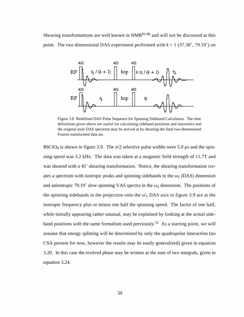
Shearing transformations are well known in NMR82-86 and will not be discussed at this

point. The two dimensional DAS experiment performed with k = 1 (37.38˚, 79.19˚) on

Figure 3.8 Redefined DAS Pulse Sequence for Spinning Sideband Calculation. The timedefinitions given above are useful for calculating sideband positions and intensities andthe original style DAS spectrum may be arrived at by shearing the final two-dimensionalFourier transformed data set.

RbClO4 is shown in figure 3.9. The /2 selective pulse widths were 5.0 µs and the spin-

ning speed was 3.2 kHz. The data was taken at a magnetic field strength of 11.7T and

was sheared with a 45˚ shearing transformation. Notice, the shearing transformation cre-

ates a spectrum with isotropic peaks and spinning sidebands in the 1 (DAS) dimension

and anisotropic 79.19˚ slow spinning VAS spectra in the 2 dimension. The positions of

the spinning sidebands in the projection onto the '1 DAS axis in figure 3.9 are at the

isotropic frequency plus or minus one half the spinning speed. The factor of one half,

while initially appearing rather unusual, may be explained by looking at the actual side-

band positions with the same formalism used previously.52 As a starting point, we will

assume that energy splitting will be determined by only the quadrupolar interaction (no

CSA present for now, however the results may be easily generalized) given in equation

3.20. In this case the evolved phase may be written as the sum of two integrals, given in

equation 3.24.

59

Figure 3.9 Sidebands in k = 1 DAS 2D Spectrum of RbClO4 at 11.7T. The pulse widthswere 5.0 µs and spinning speed was 3.2 kHz. The data was sheared with a 45˚ shearingtransformation following data collection and processing with the sequence in figure 3.6.

DAS t1, t2( ) = 1 E 2Q( ) Q , Q , 1 ,t, r1( )dt0

t1

∫

+ 1 E 2Q( ) Q , Q , 2 , t, r 2( )dt0

t2

∫(3.24)

The variables in the expressions for the energy splitting indicate that we will consider

both the absolute rotor phase and PAS orientation of the sample. Upon performing these

integrals, the DAS signal may be expressed below.

DAS t1, t2( ) = W0Q , Q ,( )t1 + W0

Q , Q ,( )t2−

WmQ , Q , 1( )

i m re

− im r t1 + r1+ Q( ) − e− im r1 + Q( )

m ≠0∑

−Wm

Q , Q , 2( )i m r

e− im r t2 + r2 + Q( ) − e

−im r 2 + Q( )

m ≠0∑

(3.25a)

60

S t1 ,t2( ) = e−i DAS t1,t2( )

= e−iW0

Q , Q , 1( ) t1e−iW0

Q , Q , 2( )t2

× expWm

Q , Q , 1( )m r

e− im r t1 + r1+ Q( ) − e

− im r1 + Q( )

m ≠0∑

× expWm

Q , Q , 2( )m r

e− im r t2 + r2 + Q( ) − e

−im r 2 + Q( )

m ≠0∑

(3.25b)

This can again be simplified with the use of delta functions as before to give the follow-

ing equation for the DAS NMR signal.

S t1 ,t2( ) = e−iW0

Q , Q , 1( ) t1− iW0Q , Q , 2( )t2

× AN1 1( )AN2

*1( )AN3 2( ) AN4

*2( )

N1,N2, N3,N4

∑

× e− i

N1−N2 +N3 −N4( ) r1+ Q( )+ N3 −N4( ) r2 − r1( )+ N1 +N3 −N4( ) r t1+ N3 r t2

AN ( ) = 12 exp iN +

WmQ , Q ,( )

m re−im

m≠0∑

d

0

2

∫

(3.26)

This may be averaged over the initial rotor phase, r1 + Q( ) , as before.

S t1, t2( )r1, Q = e

−iW0Q , Q , 1( )t1 −iW0

Q , Q , 2( )t2

× AN1 1( )AN2

*1( )AN3 2( ) AN1 −N2 +N3

*2( )

N1, N2 ,N3

∑

× e−i N2 −N1( ) r2 − r1( )+N2 rt1 +N3 r t2[ ]

(3.27)

In most cases, the relative phase of the rotor r2 − r1( ) between the first and second

evolution periods will be relatively random. In the case of large numbers of scans, these

variables r2 − r1( ) may be averaged over as well.

S t1, t2( )r1, r 2, Q = e

− iW0Q , Q , 1( )t1 −iW0

Q , Q , 2( ) t2

× AN1 1( ) 2AN2 2( ) 2

N1 ,N2

∑ e− i N1 r t1 +N2 r t2[ ] (3.28)

61

This indicates that the intensity of all of the sidebands in the two dimensional spectrum

will be positive. The peaks will occur at frequencies N1 r from W0 1( ) in the first di-

mension correlated with frequencies at N2 r from W0 2( ) in the second. When the

spectrum is sheared, the peaks will all remain positive, however their positions will shift.

Transforming the time variables into the sheared time definitions, we will arrive at the

following expression for the DAS signal.

t1 =′ t 1

k +1

t2 = k ′ t 1k +1

+ ′ t 2

(3.29a)

S ′ t 1, ′ t 2( ) = e−i

W0Q , Q , 1( )+kW0

Q , Q , 2( )( ) ′ t 1

k+1 e− iW0

Q , Q , 2( ) ′ t 2

× AN1 1( ) 2AN2 2( ) 2

N1,N2

∑ e− i

N1 r ′ t 1k+1

+kN2 r ′ t 1

k+1+N2 r ′ t 2

(3.29b)

The definition of the DAS angle pairs is equivalent to the following equation.

W0Q , Q , 1( ) + kW0

Q , Q , 2( ) = k + 1( ) iso2Q( ) (3.30)

Which reduces equation 3.29 to the form in equation 3.31.

S ′ t 1, ′ t 2( ) = e−i iso2Q( ) ′ t 1 e

−iW0Q , Q , 2( ) ′ t 2

× AN1 1( ) 2AN2 2( ) 2

N1,N2

∑ e− i

N1 r ′ t 1k+1

+kN2 r ′ t 1

k+1+N2 r ′ t 2

S ′ t 1, 0( ) = e−i iso

2Q( ) ′ t 1 AN1 1( ) 2AN2 2( ) 2

N1 ,N2

∑ e− i

N1

k+1+kN2

k+1

r ′ t 1

(3.31)

This equation shows that the isotropic spectrum arrived at by Fourier transforming the

DAS echo tops at t2 = 0 will have sidebands at multiples of two frequencies, k r k +1( )

and r k + 1( ) . The two dimensional spectrum will have sidebands at multiples of the

same two frequencies in 1 and at r in 2. Looking again at the two dimensional DAS

spectrum in figure 3.9 we observe exactly these sideband positions. Each of the slices ex-

62

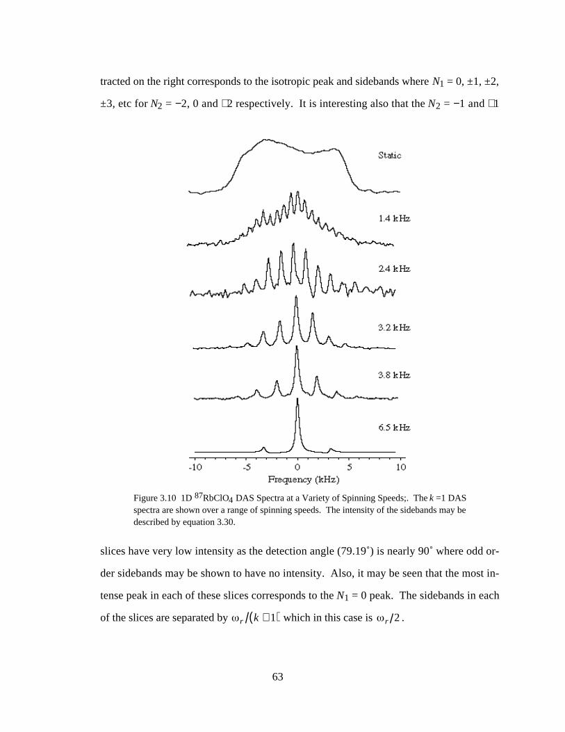
tracted on the right corresponds to the isotropic peak and sidebands where N1 = 0, ±1, ±2,

±3, etc for N2 = −2, 0 and +2 respectively. It is interesting also that the N2 = −1 and +1

Figure 3.10 1D 87RbClO4 DAS Spectra at a Variety of Spinning Speeds;. The k =1 DASspectra are shown over a range of spinning speeds. The intensity of the sidebands may bedescribed by equation 3.30.

slices have very low intensity as the detection angle (79.19˚) is nearly 90˚ where odd or-

der sidebands may be shown to have no intensity. Also, it may be seen that the most in-

tense peak in each of these slices corresponds to the N1 = 0 peak. The sidebands in each

of the slices are separated by r k + 1( ) which in this case is r 2 .

63

Figure 3.10 shows the one-dimensional DAS spectrum of 87RbClO4 taken at

11.7T at a variety of spinning rates for the usual k = 1 case just as in figure 3.9. The

sideband intensities are seen to grow more numerous and intense as the spinning speed is

reduced. The intensity of each sideband is derived from equation 3.31 by adding together

the intensity (see equation 3.33) from each N1, N2 pair which contributes an integrated

intensity of 14 AN1 1( ) 2

AN2 2( ) 2sin Qd Qd Q

0∫

0

2

∫ at a given sideband position

N1k+1 + kN2

k+1( ) r from the centerband (keeping in mind that there may be degeneracies

when k is an integer). As is the case with double rotation (DOR, see chapter 6), the

spinning sideband intensities in DAS do not necessarily approximate the static powder

pattern in the limit of very slow spinning as is the case in slow spinning MAS.

When one of the spinning angles is 0˚, as in the case of k = 5 DAS, the formula

for the DAS signal is simplified further. Since all Wn(0˚) with n ≠ 0 are zero, the value of

the intensity integrals will be simplified. In the case where 1 is 0˚, there will be side-

bands in the 1 dimension of the unsheared spectrum and all sideband intensities with N1

≠ 0 will be zero.

S ′ t 1, ′ t 2( )r1, r 2, Q = e− i iso

2Q( ) ′ t 1 e−iW0

Q , Q , 2( ) ′ t 2

× AN2 2( ) 2

N2

∑ e− i

kN2 r ′ t 1k+1

+N2 r ′ t 2

S ′ t 1, 0( )r1, r 2, Q = e− i iso

2Q( ) ′ t 1 AN2 2( ) 2

N2

∑ e−

ikN2 r ′ t 1k+1

(3.32)

A k = 5 DAS spectrum is shown below in figure 3.11. The unsheared spectrum correlat-

ing the static 0˚ spectrum with the 63.43˚ VAS spectrum shows that there are no side-

bands in the 1 dimension and the sidebands are spaced by r in the 2 dimension. In

the sheared spectrum, the sidebands in the DAS dimension are spaced by 5 r 6 and by

r in the anisotropic spectrum. This represents the highest possible effective spinning

speed in the isotropic dimension in a DAS experiment.

64

In a case where the time ratio k (or alternatively 1/k) is not an integer then the one

dimensional isotropic projection becomes more complicated. In the case of a non-integer

k, the sidebands at multiples of the two frequencies k r k +1( ) and r k + 1( ) will not

overlap for small integer values of N1 and N2. In the full two dimensional spectrum, the

sidebands will appear separated, but will not overlap when projected. This sideband be-

havior may be seen in the k = 0.8 2D DAS spectrum of RbClO4 in figure 3.12. Notice

also that there are analytically no odd sidebands in the second dimension corresponding

Figure 3.11 87RbClO4 Sidebands in k = 5 DAS 2D Spectrum. The acquisition pa-rameters are identical to those used in figure 3.7, with the exception of the angle pair (0˚and 63.43˚) used.

to odd N2. This is a direct result of spinning at 90˚ since all odd sidebands disappear in a

1D 90˚ VAS spectrum.

65

Figure 3.12 87RbClO4 Sidebands in k=0.8 DAS 2D Spectrum. The acquisition pa-rameters again are identical to those used previously, with the exception of the angle pair(39.23˚ and 90.00˚) used.

Returning to the case of one-dimensional DAS projections, the positions of side-

bands are given by equation 3.32. This equation may be integrated over the final two

powder angles, to yield an expression which may be calculated to generate sideband in-

tensities in a relatively simple manner.

S ′ t 1, 0( )powder

= e− i iso2Q( ) ′ t 1 SN1,N2 1, 2( )

N1 ,N2

∑ e− i

N1

k+1+

kN 2

k+1

r ′ t 1

SN1,N2 1, 2( ) = 14 AN1 1( ) 2

AN2 2( ) 2sin Qd Qd Q

0∫

0

2

∫(3.33)

66

This expression was used to calculate spinning sideband intensities for RbClO4 DAS

spectra with k values between 1.0 and 5.0. These simulations are shown next to the ex-

perimental spectra in figure 3.13.

Figure 3.13 All k values for fast spinning 87RbClO4 DAS at 11.7T. These spectra werecollected with experimental parameters identical to those used in the previous spectra.The simulated spectra assumed only a quadrupolar coupling CQ of 3.2 MHz, anasymmetry parameter Q of 0.10, r of 6.4 kHz and approximately 300 Hz of Lorentzianbroadening.

The quadrupolar parameters used to simulate the spectra were a CQ of 3.2 MHz, an

asymmetry parameter Q of 0.10, and a spinning speed r of 6.4 kHz. Lorentzian broad-

ening was added so that the linewidths of simulated spectra were the same as the experi-

mental spectra. It is important to note that there are basically two frequencies of spinning

sidebands in these spectra, 1k+1 r and k

k+1 r . In the case of k = 1, these two frequencies

are the same (just as was seen before in figure 3.9) and sidebands appear only at 3.2 kHz.

In the case of k = 5, the former low frequency sidebands are absent, as predicted by the-

67

ory and shown earlier in figure 3.11, and only the high frequency 5.3 kHz sidebands ap-

pear. Because the spinning speed is quite fast compared to the second-order interaction,

only the N1 = ±1 or N2 = ±1 sidebands appear in these spectra; none of the sum and dif-

ference frequencies show up.

In conclusion, the presence of spinning sidebands in DAS spectra can lead to

greatly complicated spectra, with multiple spinning frequencies present. By choosing the

proper value for the time ratio, k = 1 or k = 5, the sideband behavior is greatly simplified

and the effective spinning speed is maximized. Additionally, the sideband intensities

contain information which may be used to extract the quadrupolar coupling parameters.

This has not been discussed here and the reader is directed to the thesis of Sun16 and re-

lated papers49,52 for additional information on simulating sideband intensities.

68