Splitting and Shuﬄing: Institutional Trading Motives and ...

Splitting and Shuffling: Institutional Trading Motives

and Order Submissions Across Brokers ∗

Munhee Han† Sanghyun (Hugh) Kim‡

∗We wish to thank Vikram Nanda, Kelsey Wei, Steven Xiao, Alejandro Rivera, Kumar Venkataraman, PaulIrvine, Sang-Ook (Simon) Shin (discussant), David Lesmond(discussant), Tingting Liu(discussant), Ryan Davies,Amber Anand (discussant), Qinghai Wang, Michael Rebello, Harold Zhang, Jean-Marie Meier, and seminar partici-pants at the University of Texas at Dallas, University of Technology Sydney, Australia National University, Universityof New South Wales, the Hong Kong Polytechnic University, and conference participants at the Conference on Asia-Pacific Financial Markets 2019, Finance Down Under 2020, 6th Women in Microstructure Annual Meeting 2020,2020 FMA Virtual Conference for helpful comments. All errors are own own.

†Munhee Han ([email protected]) is at the Hong Kong Polytechnic University‡Hugh Kim ([email protected]) is at the University of Texas at Dallas

Splitting and Shuffling: Institutional Trading Motives

and Order Submissions Across Brokers

Abstract

This paper studies order submission strategies by institutional investors when trading on pri-vate information. By merging institutional daily transactions with original/confidential 13Ffilings, we separate informed trades from uninformed ones. Informed large orders tend to besplit across more brokers and over more days. While same brokers tend to work uninformedlarge orders over multiple days, the brokers who facilitated early parts of broken-up informedorders rarely receive the remaining parts of the same orders on later days. Institutional in-vestors also provide camouflage for their informed orders by mixing an informed order withother uninformed orders simultaneously sent to the same broker. As a result, a higher degree ofshuffling a portfolio of orders is associated with a larger share of informed trading volume. Thesplitting and shuffling strategies designed to conceal informed trades from brokers and othermarket participants tend to lower institutional trading costs, especially on informed orders.

Keywords: Institutional trading, informed trades, brokers, order submissions, trading costs

†Munhee Han ([email protected]) is at the Hong Kong Polytechnic University‡Hugh Kim ([email protected]) is at the University of Texas at Dallas

INSTITUTIONAL ORDER SUBMISSIONS 1

1 Introduction

In this paper we study the order submission strategies of institutional investors when they trade

on private information. Motivating the analysis is a substantial literature that models the strategies that

informed traders can use to conceal their trading motives and moderate the price impact of their trades.

Informed traders can, for instance, engage in dynamic strategies, optimally splitting orders over time to

better hide their trades among those of uninformed noisy traders (e.g., Kyle (1985), Easley and O’Hara

(1987)). Similarly, informed traders can seek opportunities and venues in which their trades can be better

concealed (e.g., Admati and Pfleiderer (1988)). Since the presence of informed trading also raises the

costs faced by uninformed traders, the uninformed traders have the incentive to certify (i.e., engage in

sunshine trading) that their trades are not information-driven (see Admanti and Pfleiderer (1991)). Seppi

(1990) suggests that uninformed traders can be screened and face lower costs trading blocks in the non-

anonymous upstairs market; whereas informed traders would split up blocks into a series of smaller orders

and trade downstairs anonymously. Consistent with the thrust of these models, this paper finds that

informed institutional traders follow order submission strategies intended to obscure their trading motives.

Institutions trading on information face the supplementary risk that their trading will be recognized

and mimicked by other traders. Several recent empirical papers have raised concerns about the private

information being detected by other market participants such as high-frequency traders (HFTs) or being

leaked through brokers to other investors. Korajczyk and Murphy (2019) find that high-frequency traders

submit more same-direction orders during institutional trade executions. Using Swedish equity data, Van

Kervel and Menkveld (2019) present evidence that HFTs supply liquidity at the beginning, but eventually

trade in the same direction as the institutions submitting the original orders. These papers argue that

such “back-running” is costly to institutional investors trading on private information. Di Maggio et al.

(2019) highlight the brokers’ role in facilitating back-running by showing that brokers can extrapolate large

informed trades from order flows and selectively leak this information to their important clients. Recently,

Yang and Zhu (Forthcoming) propose that informed traders can randomize their order flows to prevent

other traders from back-running on their fundamental information.

INSTITUTIONAL ORDER SUBMISSIONS2

There are several key findings in the paper regarding the order submission strategies of informed in-

stitutional investors. wefind that institutional investors tend to spread out their orders across more brokers

and over more days when they are trading on information. Institutional investors appear to randomize

among brokers when submitting information-driven orders. Institutional investors not only shuffle their

order flows across brokers, but also appear to submit their informed orders “camouflaged” among several

other uninformed orders when submitting information-driven orders to a broker. Furthermore, this paper

provides evidence that splitting and shuffling strategies, apparently designed to hide information from bro-

kers and other investors, lead to lower trading costs as measured by implementation shortfall, especially

on informed orders.

Our empirical analysis requires separating informed trades from uninformed ones to analyze the order

submission strategies of institutional investors trading on private information. Following Agarwal et al.

(2013), wefirst identify “confidential” holdings by merging and comparing original 13F filings with the

amendments to the original filings. 13F investors can request confidential treatment for certain holdings,

which can be omitted in the original 13F filings and reported later in the amendment filings. Agarwal et al.

(2013) show that confidential holdings of institutional investors (especially hedge funds) are information-

motivated and tend to outperform the other holdings.1 Next, wematch the managers from the ANcerno

institutional trading dataset with 13F managers based on the overlap between quarterly trades inferred

from both datasets. We manually verify the potential matches based on manager names. Then, we merge

ANcerno daily transactions with original/confidential 13F holdings reports. We identify any buy trades as

informed (uninformed) if the stocks bought during a quarter can be matched with confidential (original)

holdings for that quarter. This process allows for informed trades to be separated from uninformed ones.

We only consider buys because short positions are typically not reported in the 13F filings.

In order to examine how institutional investors break up large orders and spread them across brokers1Section 13(f) of the Securities Exchange Act of 1934 requires institutional investors to disclose their quarterly

portfolio holdings to public. Form 13F filings reports holdings information as of each calendar quarter-end andForm 13F must be filed within forty-five days of the report date. However, investment managers may request theconfidential treatment for certain holdings and omitting those holdings from Form 13F filings would be allowed untilSEC makes a decision on the request.


and over time, we stitch together all child orders that are part of the same parent orders following Anand

et al. (2012). Specifically, we stitch together all orders on the same stock on the same side of the market

(buy or sell) by the same manager on behalf of the same client (simply referred to as client-manager or

investment manager hereafter) that are executed through multiple brokers and over multiple consecutive

trading days to construct parent orders. A parent order is a collection of child orders (tickets) on the same

stock in the same direction that a fund may place with multiple brokers and over multiple days.

First, we find that investment managers tend to split their informed orders so that any given broker

may not know the full size of the orders. Specifically, we find that informed trades are more spread out

across more brokers over more trading days. This finding is more pronounced when we restrict our analysis

to large orders (blocks), defined as parent orders with share volume greater than or equal to 10,000 shares

or dollar volume greater than or equal to $200,000. Informed trades are not only spread out across a larger

number of brokers, but they are also spread out more evenly across brokers, as measured by the Herfindahl-

Hirschman Index (HHI) of dollar volume executed by each broker.2 A concern is that our results could be

driven by order size: informed orders could be larger and larger orders may simply require more brokers

and take longer time to fill. However, our results are robust to controlling for order size.3

In addition to splitting and spreading out, we find that investment managers also camouflage their

informed orders by mixing an informed order with other uninformed orders that are sent to the same

broker on the same day. Interestingly, the brokers receiving informed orders not only receive orders on a

larger number of stocks, they also receive a more evenly distributed volume of orders across stocks – so

that informed orders are not readily distinguishable from uninformed ones. These results indicate that

investment managers attempt to create their own noisy orders so as to hide their trading motives.

These order submission strategies that appear to be designed to conceal informed trades at the

individual order level further lead to a high degree of randomization of order flows on a portfolio of orders2HHI is calculated by squaring the portion of the traded aggregate dollar volumes through each broker for the

fund and then summing the resulting numbers.3We use three measures of the size of a parent order: the logarithm of the dollar volume of the parent order,

the share volume of the parent order scaled by the daily trading volume reported in Center for Research in SecurityPrices (CRSP), and the share volume of the parent order scaled by the number of shares outstanding reported inCRSP.


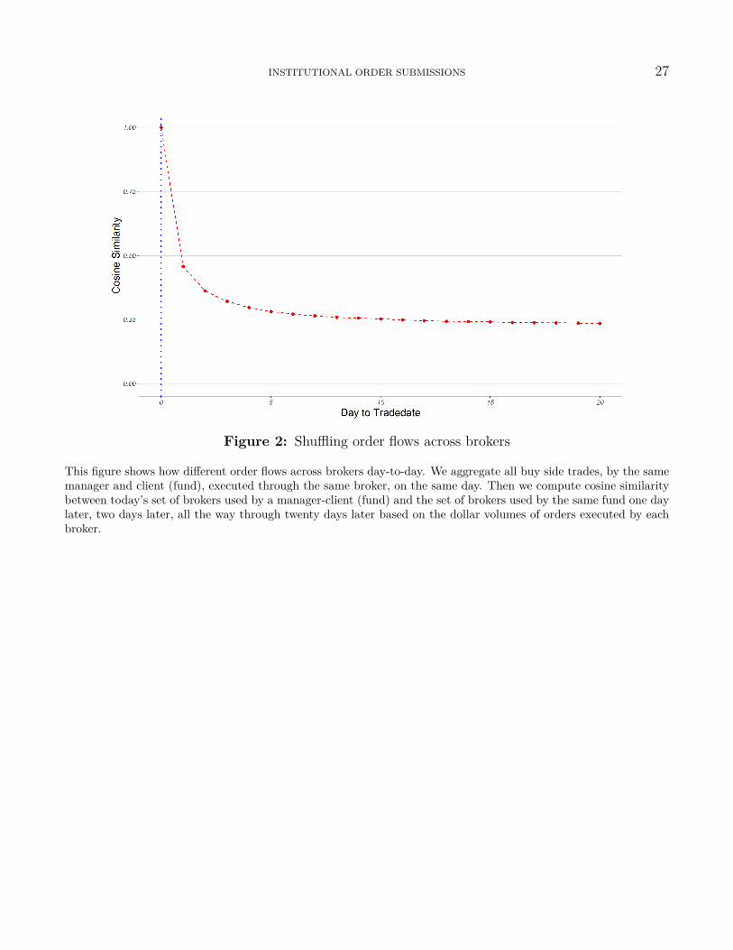
sent across brokers. To show this, we aggregate for each client-manager all buy orders executed on the same

day to construct a portfolio of orders on a daily basis. Then, we measure the extent to which a set of brokers

used by an investment manager tend to overlap with or deviate from the set of brokers that the investment

manager has used in the past. We ask, for instance, if manager m submits her largest volume of orders to

broker b today, would broker b also receive the largest order flows from manager m tomorrow? Specifically,

we measure the similarity between the set of brokers used by an investment manager today and the set

of brokers used by the same manager one day later, two days later, up to twenty days later. The broker

similarity is measured by cosine similarity based on the dollar volume of orders executed by each broker.

We find that investment managers tend to submit their orders to a slightly different set of brokers each

day. Looking across days that are further apart, the cosine similarity of the brokers used by each manager

drops initially, but settles to a steady level in just a few days. This suggests that while shuffling order

flows sent across brokers to hide informed orders, investment managers typically maintain close trading

relationships with their core sets of brokers, that can facilitate liquidity provision when managers submit

large liquidity-motivated orders (Han, Kim, and Nanda (2019)).

Next, we investigate why investment managers shuffle their orders across brokers each day. One

reason for shuffling could be to maintain premium status with a large number of brokers and obtain

valuable services such as access to sell-side research (Goldstein et al. (2009)). If a manager does not have

a sufficient volume of orders to split on any given day, the manager may take turns submitting orders to

different brokers in order to maintain close relationships with a large number of brokers. We argue that an

alternative important motive for shuffling is to conceal informed orders. To test this, we measure similarity

between today’s set of brokers used by an investment manager and the core set of brokers used by the

manager (from day t-25 to day t-6), as measured by cosine similarity based on the aggregate dollar volume

of orders executed by each broker. We find that there is a larger share of informed trading volume on

days when investment managers deviate from their core sets of brokers, that is, when the broker similarity

is lower and the degree of shuffling is higher. This result is generally consistent with the randomization

strategy envisioned in Yang and Zhu (Forthcoming) that investment managers can shuffle their order


flows in order to conceal their informed orders. Again, a concern may be that investment managers trade

larger quantities of shares on days with more informed trading volume and are naturally forced to send

orders outside their core sets of brokers. However, the results are robust to controlling for trading volume,

mitigating this concern.

So far our analysis has been limited to ANcerno client-managers for which ANcerno managers could be

matched with 13F managers and limited to manager-quarters with confidential 13F filings. As a robustness

check, we extend this analysis to the full ANcerno sample. On every trading day we sort funds into quintile

based on cosine similarity of the dollar volume of orders executed by each broker between the set of brokers

used today by a fund and the core set of brokers used by the same fund (from day t-25 to day t-6). Then

we measure the value-weighted buy-and-hold return on the stocks bought on each day by each client-

manager, weighted by dollar volume, for the next month (typically from day t+1 to day t+21). For each

quintile, we first average value-weighted returns across client-managers and then use the time series average

value-weighted returns for statistical inference in the spirit of Fama and MacBeth (1973), adjusting for

serial correlation up to a lag of 20 trading days following Newey and West (1987). We find that the

most dissimilar quintile outperforms the most similar quintile by 24 basis points per month (t = 3.20).

When adjusting for DGTW-benchmark returns (Daniel et al. (1997)), the return spread remains large and

statistically significant at 17 basis points per month (t = 2.77). This full sample result corroborates the

previous finding that investment managers shuffle their orders across brokers more on days with a larger

share of informed trading volume.

An important question that remains is whether the splitting and shuffling strategies work for invest-

ment managers in terms of reducing trading costs on informed orders. Following the literature (e.g., Anand

et al. (2012), Anand et al. (2013)), we measure institutional trading costs using the implementation short-

fall. First, we examine individual parent orders. We find that splitting orders across brokers on any given

day tends to reduce trading costs for informed orders, whereas splitting uninformed orders has little effect

on implementation shortfall. Since the first day portion of multi-day orders could be larger than the later

day portions, which could affect both splitting decisions and trading costs, we control for order-sequence


fixed-effects (first day, second day, etc.). The result is robust to controlling for various fixed-effects and

order size. Next, we restrict our analysis to multi-day orders (about 30% of parent orders) in order to

examine how orders are sequenced and shuffled across brokers over time. Investment managers may avoid

sending remaining parts of the large informed orders to the brokers that executed early parts of the orders

in order to conceal the underling informed trading motives. Consistent with this prediction, sending later

parts of the orders to new brokers (i.e., shuffling) tends to lower trading costs on informed orders. Again,

this result is robust to controlling for various fixed-effects and order size.

Finally, we examine portfolios of orders at a daily level to test whether the shuffling strategy at the

macro level works for investment managers. We find that dis-similarity between today’s set of brokers used

by a fund and the core set of brokers used by the same fund (one minus cosine similarity) is associated with

lower trading costs as measured by implementation shortfall on informed orders. The result, combined

with the earlier results, is consistent with investment managers shuffling informed orders across brokers

and mixing informed orders with other uninformed orders sent to the same brokers, in order to mitigate

trading costs on informed orders.

The remainder of the paper is organized as follows. Section 2 describes the data sources and the

construction of our sample and variables. We report our results in Section 3. Section 4 concludes.

2 Data and Variable construction

Our analysis of order submission strategies across brokers by informed traders exploits a detailed

trade-level dataset that also contains information on institutional investors and their brokers. Another

important requirement of our analysis is identifying whether a trade is information-motivated or not. We

describe the institutional daily transaction data and how we construct our sample, and then explain how

we identify informed trades.

We obtain institutional daily transactions from ANcerno data (also known as Abel Noser data).4

4Other recent studies using ANcerno data to examine the behavior of institutional investors include Chemmanur,He, and Hu (2009); Chemmanur, Hu, and Huang (2010), Goldstein et al. (2009), Goldstein, Irvine, and Puckett (2011),Puckett and Yan (2011), Anand et al. (2012, 2013), Hu et al. (2014), Jame (2018), Barbon et al. (Forthcoming),


Our data cover equity transactions made by a large sample of institutions from January 1999 through

December 2009. For each transaction, the data include the date of transaction, the stock traded (identified

by both ticker and CUSIP), the number of shares traded, whether it is a buy or sell by the institution,

the transaction price, various benchmark prices, the broker executing the trade, and commissions paid to

the broker. Using an algorithm similar to the ones used in Hu et al. (2018) and Choi et al. (2016), we

match ANcerno managers (identified by managercode) and 13F managers (identified by CIK) by comparing

quarterly changes in holdings computed from ANcerno data and 13F filings. In addition, ANcerno provided

the names of investment managers in 2011. This enables me to use the manager names to manually verify

the manager matches from ANcerno daily transactions database and 13F quarterly holdings reports.

Institutional investors tend to break up large orders and spread them across brokers and over time.

In ANcerno data, observation units are those broken-up child orders, called tickets. Following Anand et al.

(2012), we stitch together all child orders that are part of the same parent orders. Specifically, we stitch

together all tickets on the same stock on the same side of the market (buy or sell) by the same manager on

behalf of the same client (referred to as client-manager or investment manager hereafter) that are executed

through multiple brokers over multiple consecutive trading days to construct parent orders. A parent order

is just a collection of child orders on the same stock in the same direction that an investment manager

may place with multiple brokers over multiple trading days.

Next, we identify informed trades using “confidential” 13F filings, following Agarwal et al. (2013). We

directly retrieve both original 13F filings and all amendment filings (Form 13F-HR and Form 13F-HR/A5)

dated between March 1999 and December 2009 from the SEC’s Electronic Data Gathering, Analysis, and

Retrieval (EDGAR) system. For the sake of data consistency and integrity, we extract information about

the original 13F holdings directly from the EDGAR, rather than using Thomson Reuters’ 13F institutional

holdings database (s34). Amendments to 13F filings provide two types of information: (1) a change in a

position that was reported in the original 13F filing and (2) a newly added position that was not reported

Ben-Rephael and Israelsen (2018), and Di Maggio et al. (2019).5Form 13F-HR/A includes an indication on its cover regarding whether it is an “amendment” (i.e., whether it

adds new holdings) or a “restatement.” We only include forms with the “amendment” box checked.


in the original 13F filing. We define a holding as a “confidential” holding if there is a positive change

in the position on the original filing or if it is a newly added position on an amendment filing. We note

that a vast majority of confidential holdings are newly added positions that are disclosed later on the

amendment filings. Figure 1 provides a timeline of the original and amendment 13F filings. We define

any buy transaction from the ANcerno-13F merged dataset during a quarter as an informed (uninformed)

trade if it can be matched with a confidential (original) holding at the quarter-end. We only consider buys

because short positions are typically not reported in the 13F filings.

[Insert Figure 1]

Our initial manager matching process gives rise to 129 ANcerno-13F managers. Out of those 129

managers, 61 managers have at least one quarter with confidential holdings. About 6 % of parant orders

are considered informed orders. Panel A of Table 1 describes the characteristics of the parent orders.

Parent orders are, on average, split across 1.74 brokers and over 1.38 trading days. Panel B of Table 1

describes the characteristics of the daily portfolios of orders.

[Insert Table 1]

Next, we measure the extent to which investment managers shuffle their order flows across brokers

by the broker dis-similarity. First, we aggregate the dollar volume of buy orders on the same day by the

same client-manager executed by each broker. Then, we calculate the cosine similarity between today’s

set of brokers used by an investment manager and the core set of brokers used by the same manager (from

day t − 25 to day t − 6) based on the dollar volume of buy orders executed by each broker. This proxy

captures how similar today’s set of brokers used by an investment manager is to the set of brokers used by

the same manager in the past 20 days, skipping the 5 days immediately preceding the current day. The

broker dis-similarity is just one minus cosine similarity.

For a robustness check, we construct two additional measures to capture patterns of order flow

shuffling across brokers. First, like the first measure, we aggregate the dollar volume of orders across the

same client-manager and across each broker on the same day. we then consider the overlapping percentage


volume executed by the brokers today and the brokers in the past 20 days (from day t− 25 to day t− 6).

Second, we consider only one broker who executed the largest dollar volume for each client-manager during

the past 20 days (t− 25 to day t− 6). we then calculate the fraction of today’s dollar volume executed by

the top broker based on the dollar volume in the past 20 days. If an investment manager keeps submitting

orders to the same brokers, then there will be little shuffling and the broker similarity (dis-similarity) will

be high (low). On the other hand, if an investment manager keeps submitting orders to different brokers,

then there will be a lot of shuffling and the broker similarity (dis-similarity) will be low (high).

In order to examine how the order splitting and shuffling strategies affect institutional trading costs,

we construct the implementation shortfall measure (the percentage change between the execution price and

the benchmark price) at the ticket level. Specifically, following Keim and Madhavan (1997) and Anand

et al. (2012, 2013), we calculate implementation shortfall as follows:

P1(t) − P0(t)P0(t) ×D(t) (1)

where P1(t) is the volume-weighted execution price, P0(t) is the benchmark price prevailing at the time

when a broker receives the order, and D(t) is the sign of the trade (+1 for a buy and −1 for a sell).

3 Order Submission Strategies

We begin our empirical analysis by examining order submission strategies at the parent-order level

in Section 3.1 and turn to examining order submission strategies at the portfolio level in Section 3.2. we

first show how institutional investors place orders differently when trading on private information and then

examine how the order submission strategies across brokers can affect institutional trading costs.

3.1 Analysis of Parent Orders

Following Anand et al. (2012), we stitch together all orders on the same stock on the same side

of the market by the same client-manager that are executed through multiple brokers and over multiple


consecutive trading days to construct parent orders. A parent order is just a collection of child orders

(tickets) on the same stock in the same direction that an investment manager may place with multiple

brokers over multiple trading days. We contend that, when trading on private information, institutional

investors may spread their orders across more brokers and over more trading days in order to conceal

their informed trading motives. As discussed in Section 1, this splitting strategy is consistent with many

theoretical models of informed trading, starting with Kyle (1985) and Easley and O’Hara (1987).

In order to test this hypothesis, we identify information-motivated orders by combining ANcerno

daily transactions with 13F quarterly holdings (both original and confidential). Specifically, a parent buy

order during a quarter that can be matched with a holding at the end of the quarter for which an investment

manager has sought confidentiality treatment is identified as an informed trade. In other words, informed

buy orders end up appearing on the manager’s confidential 13F filings, but not on the original 13F filings,

whereas uninformed buy orders end up appearing on the manager’s original 13F filings on the report

date at the end of the quarter. Intuitively, an attempt to hide their positions by seeking confidentiality

treatment implies that managers have traded those stocks acting on their superior private information.

Indeed, Agarwal et al. (2013) show that confidential holdings tend to outperform original holdings.

Having separated information-motivated orders from uninformed ones, we estimate the following

linear regression model:

Number of Daysi,k,s,t = β × 1(Informed Motivatedi,k,s,t) + αi,k + ρs + θt + εi,k,s,t (2)

where i indexes managers, k indexes clients, s indexes stocks, and t indexes dates on which parent orders

were initially placed. The dependent variable is the number of days for which parent orders are extended

(Number of Daysi,k,s,t) or the number of brokers to which parent orders are sent (Number of Brokersi,k,s,t)

or the broker’s Herfindahl-Hirschman Index (Broker HHI i,k,s,t), which measures the degree of concentration

(or diversification) across brokers to which a parent order is sent, calculated by squaring a fraction of

the dollar volume executed by each broker and summing it over all brokers to which a parent order is

submitted. The independent variable of interest, 1(Informed Motivatedi,k,s,t), is an indicator variable that


takes the value of one if a parent order is motivated by information and zero otherwise. Depending on

the specification, the regression includes client-manager fixed effects (αi,k) and stock fixed effects (ρs). All

regressions include time fixed effects (θt), and standard errors are clustered by client-managers.

The baseline regression results are presented in Panel A of Table 2. In columns (1) and (2), the

dependent variable is Number of Daysi,k,s,t. In column (1), the coefficient of 1(Informed Motivatedi,k,s,t)

is positive and statistically significant at the 1% level. This is consistent with our hypothesis that in-

stitutional investors are more likely to split their order across multiple days when trading on private

information. The result remains largely unchanged when controlling for stock fixed effects in column (2).

In columns (3) and (4), the dependent variable is Number of Brokersi,k,s,t. In column (3), the coefficient

of 1(Informed Motivatedi,k,s,t) is positive and statistically significant at the 1% level. This suggests that

institutional investors tend to place orders across more brokers when the orders are motivated by pri-

vate information. Also, the result remains robust when controlling for stock fixed effects. In columns (5)

and (6), we replace Number of Brokersi,k,s,t with Broker HHI i,k,s,t in the above linear regression model.

Broker HHI measures the degree of concentration across brokers to which a parent order is sent and is

calculated by squaring a fraction of the dollar volume executed by each broker and summing it over all

brokers to which a parent order is submitted. A lower Broker HHI implies that a parent order is spread

out across a more diversified set of brokers. we contend that informed orders are more likely to be sent

across a diversified set of brokers in order to hide the information content of the orders from the brokers

and other market participants. In columns (5) and (6), 1(Informed Motivated) is negatively associated

with Broker HHI and statistically significant at 1%, with or without controlling for stock fixed effects.

This implies that informed orders are sent in a scattered way across brokers when compared to uninformed

orders.

One might be concerned that our results could be driven by order size. In other words, informed

orders could be larger, and larger orders may require more days and more brokers to fill. In order to address

this concern, we re-run the tests in a sub-sample of large orders (“blocks”), defined as parent orders with

share volume greater than or equal to 10,000 shares or dollar volume greater than or equal to $200,000.


The regression results are presented in Panel B of Table 2. We continue to find qualitatively similar, even

stronger, results that large informed orders are spread over more days and sent across more brokers than

large uninformed orders. In addition, we control for several proxies to control for effects related to order

size: log of dollar volume, share volume as percentage of CRSP volume, and share volume as percentage of

the number of shares outstanding. The results are reported in Panel C, Panel D, and Panel E, respectively.

We continue to obtain qualitatively similar results.

[Insert Table 2]

From the previous analysis, we find that institutional investors tend to spread out their informed

orders across more brokers and over more trading days. An important question that remains is whether

such order submission strategies work for institutional investors in terms of reducing trading costs. We

argue that if they are effective in concealing informed trading motives, those order submission strategies

should reduce trading costs on informed orders. We compute the implementation shortfall, which is the

percentage change between the execution price and a benchmark price as the transaction cost (Keim and

Madhavan (1997) and Anand et al. (2012, 2013)).

In order to test whether splitting orders across brokers are effective in reducing trading costs, we

estimate the following linear regression model:

Implementation Shortfalli,k,s,b,d,t = δ × 1(Informed Motivatedi,k,s,t) × 1(Multiple Brokersi,k,s,t)

+ β × 1(Informed Motivatedi,k,s,t) + λ× 1(Multiple Brokersi,k,s,t)

+ αi,k + γd + ρs + ηb + θt + εi,k,s,b,d,t

(3)

where i indexes managers, k indexes clients, s index stocks, b indexes brokers, and t indexes trading days.

The dependent variable, Implementation Shortfalli,k,s,b,t, is the percentage difference between the execution

price and the benchmark price. As before, 1(Informed Motivatedi,k,s,t) is an indicator variable that takes

the value of one if the order is driven by information. 1(Multiple Brokersi,k,s,t) is an indicator variable

that takes the value of one if the order is split up across multiple brokers on that trading day and zero

otherwise. Depending on the specification, the regression includes client-manager fixed effects (αi,k), stock


fixed effects (ρs), broker fixed effects (ηb), and time fixed effects (θt). All regressions include order-sequence

fixed effects (γd) to control for unobserved characteristics of child orders that are executed on the first day,

second day, and so on, as part of parent orders. As before, standard errors are clustered by client-manager.

The regression results are presented in Panel A of Table 3. Consistent with our prediction, split-

ting across multiple brokers to execute an order can lower trading costs, especially on informed or-

ders. We continue to find qualitatively similar results after controlling for order size using log of dol-

lar volume in Panel B. Furthermore, when we restrict our analysis to sub-samples that only includes

multi-day parent orders in Panels C and D, we find the coefficient of the interaction term between

1(Informed Motivatedi,k,s,t) ×1(Multiple Brokersi,k,s,t) to be much greater than the one from the full sam-

ple. This result suggests that the effect of spreading out informed orders across multiple brokers on trading

costs is more pronounced when the orders extend multiple days.

[Insert Table 3]

In the previous analysis, we considered the static strategy of splitting orders across multiple brokers

on the same trading days, thus muting the time dimension. Next, we consider the dynamic strategy of

splitting orders across brokers across multiple trading days. We contend that later parts of informed

orders would be sent to different brokers from the ones that initially executed early parts of the same

parent orders. Such dynamic order splitting strategies can help prevent any single broker from learning the

full size and information content of the orders, thereby mitigating trading costs. To test this prediction,

we estimate the following linear regression model:

Implementation Shortfalli,k,s,b,d,t = δ × 1(Informed Motivatedi,k,s,t) × 1(Different Brokeri,k,s,t)

+ β × 1(Informed Motivatedi,k,s,t) + λ× 1(Different Brokeri,k,s,t)


(4)

where i indexes managers, k indexes clients, s index stocks, b indexes brokers, d indexes order-sequence, and

t indexes trading days. The dependent variable, Implementation Shortfalli,k,s,b,t, is the percentage difference

between the execution price and the benchmark price. As before, 1(Informed Motivatedi,k,s,t) is an indicator


variable that takes the value of one if the order is driven by information. 1(Different Brokeri,k,s,t) is an

indicator variable that takes the value of one if an order is sent to a different broker from the ones that

executed early parts of its parent order on the first trading day. Depending on the specification, the

regression includes client-manager fixed effects (αi,k), stock fixed effects (ρs), broker fixed effects (ηb), and

time fixed effects (θt). All regressions include order-sequence fixed effects (γd) and standard errors are

clustered by client-manager.

The regression results are presented in Table 4. The above analysis is naturally restricted to a sub-

sample of child orders that are part of multi-day parent orders and that are executed on the second day or

later days. As before, we control for order-sequence fixed effects, essentially comparing second-day informed

orders to second-day uninformed orders, third-day informed orders to third-day uninformed orders, and so

forth. Consistent with our prediction, we find that submitting later parts of informed orders to different

brokers from the ones that initially executed early parts of the same parent orders are effective in reducing

trading costs. Again, we continue to find qualitatively similar results after controlling for order size, as

shown in Panel B.

[Insert Table 4]

3.2 Analysis of Order Portfolios

In the previous subsection, we examined institutional order submission strategies at the parent-order

level. In this subsection, we extend our analysis to order portfolios and examine macro-level strategies.

First, we examine the order “camouflaging” strategy that can serve as a bridge between the analysis of

parent orders and that of order portfolios. Then, we examine the order ”shuffling” strategy at the order-

portfolio level, which combines the dynamic order splitting strategy that was considered in the previous

subsection and the order camouflaging strategy in this subsection.

Our analysis of order submission strategies at the parent-order level provides evidence that insti-

tutional investors tend to spread their orders across more brokers and over more days when trading on

information. Moreover, the order splitting strategies (both static and dynamic) tend to reduce trading


costs by enabling informed traders to conceal their trading motives. Here we examine a different type of

order submission strategy that can achieve the same goal: order camouflaging strategy. When submitting

an informed order to a broker, the informed trader may submit uninformed orders simultaneously to the

same broker, essentially creating its own noisy orders.

In order to test this prediction, we estimate the following linear regression model:

log(Number of Stocks)i,k,b,t = β × 1(Informed Order to Brokeri,k,b,t) + αi,k + ηb + θt + εi,k,b,t (5)

where i indexes managers, k indexes clients, b indexes brokers, and t indexes time in trading days. The

dependent variable, log(Number of Stocks)i,k,b,t, is the number of stocks that broker b receives from client-

manager i-k on trading day t. The independent variable of interest, 1(Informed Order to Brokeri,k,b,t)

is an indicator variable that takes the value of one if broker b receives at least one informed order from

client-manager i-k on trading day t. Depending on the specification, the regression includes includes

client-manager fixed effects (αi,k), broker fixed effects (ηb), and time fixed effects (θt). Standard errors are

clustered by client-manager.

The results are reported in Table 5. In columns (1)-(3) of Panel A, we find that investment manager

tend to submit a greater number of stocks to a broker to whom they submit informed orders. Moreover,

we find similar results after controlling for order size using log of dollar volume in columns (4)-(6). As a

robustness check, we replace log(Number of Stocks)i,k,b,t with Stock HHIi,k,b,t. Stock HHIi,k,b,t is calculated

by squaring the fraction of the dollar volume traded on each stock and then summing up across all stocks

that a broker receives. The results suggest that when submitting an informed order to a broker, the

informed trader tends to submit a more evenly distributed portfolio of orders in terms of dollar volume.

These strategies are consistent with the institutional investors attempting to hide informed orders by

creating their own noisy orders.

[Insert Table 5]

Order submission strategies designed to hide informed trades at the individual order level also lead


to a large degree of randomization of order flows across brokers at the order portfolio level. To see how

institutional investors keep submitting their orders to different brokers over time, we measure the extent

to which a set of brokers an investment manager uses overlap with or deviate from the set of brokers the

same manager has used in the past. Specifically, we measure the cosine similarity between today’s set of

brokers used by an investment manager and the set of brokers used by the same manager one day later, two

days later, all the way through twenty days later, based on the dollar volume of orders executed by each

broker. Figure 2 shows that investment managers tend to submit their orders to a slightly different set of

brokers every day. Looking across days that are further apart, the broker similarity further drops, but at a

decreasing rate, and starts to converge in a few days. This suggests that while shuffling order flows across

brokers to hide informed orders, investment managers typically maintain close trading relationships with

their core sets of brokers, since brokerage connections can help mitigate trading costs on large liquidity-

motivated orders (Han, Kim, and Nanda (2019)).

[Insert Figure 2]

An important question at this point is why institutional investors shuffle their order flows across

brokers everyday. One reason could be to maintain premium status with a large number of brokers and

receive valuable services such as access to sell-side research (Goldstein et al. (2009)) Another important

motive for shuffling could be to hide informed orders from the brokers. To answer this question, we examine

whether a degree of order shuffling is associated with an extent of informed trading volume. To this end,

we measure the broker dis-similarity between today’s set of brokers used by a client-manager and the core

set of brokers used by the same manager (from t − 25 to day t − 6), as measured by one minus cosine

similarity based on the dollar volume of orders executed by each broker. Then, we estimate the following

linear regression model:

Dis-similarityi,k,t = β × 1(Informed Sharesi,k,t > 0.5) + αi,k + θt + εi,k,t (6)

where i indexes managers, k indexes clients, and t indexes time. The dependent variable, Dissimilarityi,k,t,


is one minus cosine similarity of broker usage of today and that from day t − 25 to day t − 5. The

independent variable of interest, 1(Informed Sharesi,k,t > 0.5) is an indicator variable that takes the value

of one if more than half of dollar trading volume is driven by information. Depending on the specification,

the regression includes client-manager fixed effects (αi,k) and time fixed effects (θt) and standard errors

are clustered by client-manager.

The regression results are presented in Panel A of Table 6. In column (1), the coefficient of

1(Informed Sharesi,k,t > 0.5) is positive and statistically significant at the 1% level, which is consistent

with our prediction that there is a higher degree of order shuffling across brokers on days with a larger

share of informed trading volume. This result remains robust when controlling for time fixed effects in

column (2). A possible concern about our results is that large orders can make investors order through

various brokers, which can lead to higher dissimilarity. we control for log of dollar volumes, the number of

shares traded, and the number of stocks traded on the same day to mitigate the concerns about order size.

We find qualitatively similar results after controlling for these proxies for the order size in columns (4)-(6).

Similarly, we provide additional robustness checks by constructing more measures of dissimilarity.

The first measure is one minus the overlapped dollar volumes traded through the set of brokers used by an

investment manager and the set of brokers used by the same manager in the past. For the third measure,

we compute how much the manager-client trades through their top broker, which is chosen based on the

trading information from 25 to 5 days before the current day (i.e., today). We replace cosine similarity

with the computed measure. These results are reported in Panel B and Panel C of Table 6, respectively.

Our results are robust when we use different measures of dissimilarity.

[Insert Table 6]

By research design, our analysis is limited to ANcerno manager-client pairs (funds) where ANcerno

managers can be matched with 13F managers and manager-quarters when confidential filings. We extend

the previous analysis to the full ANcerno sample. We examine the effect of the randomization strategy

across brokers on performance. Every trading day we sort funds into quantiles based on similarity based

on cosine similarity based on the dollar volume of orders executed by each broker between today’s set of


brokers used by a fund and the core set of brokers used by the same fund (from day t-25 to day t-6).

Then we measure the value-weighted buy-and-hold return on the stocks bought on each day by each fund,

weighted by dollar volume, for the next month (typically from day t+1 to day t+21). For each quintile, we

first average value-weighted returns across funds then use the time series average value-weighted returns for

statistical inference in the spirit of Fama and MacBeth (1973) and adjust for serial correlation up to a lag

of 20 trading days following Newey and West (1987). We find that the most dissimilar quintile outperform

the most similar quintile by 24 basis points per month (t = 3.20). When adjusting for DGTW-benchmark

returns (Daniel et al. (1997)), the return spread remains large and statistically significant at 17 basis points

per month (t = 2.77). This full sample result corroborates the previous finding that investment managers

shuffle their orders across brokers more on days with a larger share of informed trading volume.

[Insert Table 7]

When institutional investors are trading on their private information, they believe that the informa-

tion will eventually be publicly disclosed and the price will reflect the information, accordingly. However,

they want to maximize their possible profits from this information. The primary prediction that we can

derive from our hypothesis is that a randomization strategy across brokers can deter brokers from leaking

private information, thereby reducing trading costs on informed orders. we compute implementation short-

fall which is the percentage difference between the execution price and a benchmark price as transaction

costs. (Keim and Madhavan (1997) and Anand et al. (2012, 2013)) This measure is at manager-client-stock-

broker-day. Then, we interact dissimilarity measure with the indicator variable for identifying information

motivated trade and estimate the following linear regression model:

Implementation Shortfalli,k,s,b,t = δ × 1(Informed Motivatedi,k,s,t) × Dissimilarityi,k,t

+ β × 1(Informed Motivatedi,k,s,t) + λ× Dissimilarityi,k,t

+ αi + γk + ρs + ηb + θt + εi,k,s,b,t

(7)

where i indexes managers, k indexes clients, s index stocks, b indexes brokers, and t indexes time in day.

The dependent variable Implementation Shortfalli,k,s,b,t, is the percentage difference between the execution


price and a benchmark price. The independent variable of interest, 1(Informed Motivatedi,k,s,t) denotes

whether the order is driven by informed reason or not and Dissimilarityi,k,t is 1−cosine similarity between

the set of manager-client’s aggregate trading dollar volume through its broker at today and that from 25

days before to 5 days before today. Depending on the specification, the regression includes manager ×

client (fund) fixed effects (αi,k), stock fixed effects (ρs), and broker fixed effects (ηb). All regressions include

time fixed-effects (θt) and standard errors are clustered by manager × client.

Panel A of Table 8 reports the results. Consistent with our prediction, we find a negative and

statistically significant coefficient on 1(Informed Motivatedi,k,s,t) × Dissimilarityi,k,t and we continue to

find the robust results after using different specifications including several fixed effects in columns (1)-(3).

The estimates are also economically significant as the implementation shortfall decrease at around 12 bps.

In contrast, the coefficients on 1(Informed Motivatedi,k,s,t) are positive and statistically significant. The

results suggest that more randomizing order flows across brokers can reduce the execution cost by hiding

the true intention of order. Moreover, even though the coefficient on Dissimilarityi,k,t is not statistically

insignificant, it is positive. Potentially, it can be interpreted as that more shuffling order flows across

brokers can be relatively more expensive, thereby increase transaction costs. Moreover, we re-run the

regression by using sub-sample which includes block orders (the aggregate volume of trade is greater than

equal to 10,000 shares or the aggregate dollar volumes of trade is greater than equal to $200,000). Then

we continue to obtain qualitative similar but much stronger magnitude of coefficients in columns (4)-(6).

Since trading volume can not only impact on price but also can contain information itself, we control

for order sizes by using several proxies capture effects of order size. They are log of dollar volumes, log

of volumes, percentage of shares traded in CRSP volume, and percentage of shares traded in outstanding

shares. The results are reported in Panel B and C respectively. We continue to obtain qualitatively similar

results.

[Insert Table 8]


3.3 Robustness Checks

In this subsection, we demonstrate the robustness of our main results regarding splitting and shuffling

strategy by extending sample to the full ANcerno sample. For the main results, we separate information-

motivated orders from uninformed ones by matching ANcerno transaction data with confidential 13F filings.

Unfortunately, this process results in a large loss of data, as it requires matching ANcerno managers and

13F managers, yet not all ANcerno-13F matched managers seek confidentiality treatment on their holdings.

Therefore, we extend the analysis to the entire ANcerno dataset to corroborate our main findings by using

a different proxy to identify informed orders. Form 13F requires that all investment managers who have

investment discretion over $100 million or more in Section 13(f) securities to disclose their quarter-end

holdings in these securities (Agarwal et al. (2013)). If private information arrives near the quarter end, an

investment manager might want to delay building a large position until the new quarter starts in order to

avoid prematurely reporting a new informed position. In addition, investment managers may exert more

effects into acquiring private information early in the quarter for the same reason. Hence, investment

managers are likely to trade more heavily on private information earlier in the quarter. Based on this

understanding, we estimate the following linear regression model:

Number of Daysi,k,s,t = β × Days to Quarter-endi,k,s,t + αi,k + ρs + θt + εi,k,s,t (8)

where i indexes managers, k indexes clients, s indexes stocks, and t indexes first trading days on which

parent orders were placed. The dependent variable is the number of days for which parent orders extend

(Number of Daysi,k,s,t) or the number of brokers to which parent orders are sent (Number of Brokersi,k,s,t)

or broker Herfindahl-Hirschman Index (Broker HHI i,k,s,t) which measures the degree of concentration

across brokers to which a parent order is sent, calculated by squaring a fraction of the dollar volume

executed by each broker and summing it over all brokers to which a parent order is submitted. The inde-

pendent variable of interest, Days to Quarter-endi,k,s,t, is the number of days from the first day on which

a parent order is submitted to the calendar quarter-end. Depending on the specification, the regression


includes manager×client (fund) fixed-effects (αi,k), stock fixed-effects (ρs) and quarter fixed-effects (θt).

Standard errors are clustered by manager × client (fund) for all regressions.

The results are reported in Panel A of Table A1. In columns (1) and (2), the coefficient of

Days to Quarter-endi,k,s,t is positive and statistically significant at the 1% level, controlling for various

fixed effects. This suggests that trade orders executed early in the quarter (presumably informed orders)

require more days to complete. In columns (3) and (4), the coefficient of Days to Quarter-endi,k,s,t is

positive and statistically significant, implying that orders tend to be placed across more brokers earlier in

the quarter. From columns (5) and (6), we replace Broker HHI i,k,s,t with Broker HHI i,k,s,t. We find that

trades in the earlier period of the quarter are more likely to be sent across a diversified set of brokers.

In order to mitigate concerns that our results could be driven by order size, we re-run the same linear

regression in a sub-sample of large orders. However, the results reported in Panel B of Table A1 remain

qualitatively similar and somewhat stronger. Overall, the results suggest that informed orders identified

as those executed early in the quarter are likely spread over more days across more brokers and consis-

tent with our prediction that investment managers attempt to conceal information content of orders from

the brokers. As a robustness check, we control for several measures of order size: log of dollar volumes,

percentage of shares traded in CRSP volume, and percentage of shares traded in outstanding shares. The

results are reported in Panel C, Panel D, and Panel E, respectively. We continue to obtain qualitatively

similar results.

[Insert Table A1]

Examining trades executed during the earlier period of quarter is allowing me not to lose lots of

observations. Hence, we regress Dissimilarityi,k,t on Days to Quarter-endi,k,t including various fixed effects

in the following linear regression model:

Dissimilarityi,k,t = β × Days to Quarter-endi,k,t + αi,k + θt + εi,k,t (9)

where i indexes managers, k indexes clients, and t indexes time. The dependent variable Dissimilarityi,k,t,


is 1−cosine similarity between the set of manager-client’s aggregate trading dollar volume through its

broker at today and that from 25 days before to 5 days before today. The independent variable of interest,

Days to Quarter-endi,k,t is the number of days from the first day of order to quarter-end. Depending on the

specification, the regression includes manager × client (fund) fixed effects (αi,k), and time fixed-effects (θt)

and standard errors are clustered by manager × client. The regression results are presented in Table A2.

For all three proxies, we find that trades executed early in the quarter (presumably informed orders) tend

to randomize their order flows across brokers. This evidence supports our hypothesis that investors are

more likely to shuffle order flows across brokers when they are trading on their private information. This

result is robust after controlling for various fixed effects and controlling daily aggregate dollar volumes, the

number of shares traded, and the number of stocks traded.

[Insert Table A2]

4 Conclusion

In this paper, we study order submission strategies by institutional investors when trading on private

information by exploiting proprietary data on institutional daily transactions. we separate informed orders

from uninformed order by using 13F confidential holdings following Agarwal et al. (2013). We find that

institutional investors tend to split orders over more days to complete the order and across more brokers

when they are trading on private information. Furthermore, while institutional investors place uninformed

large orders to the same brokers over multiple days, they tend to submit informed orders after the first

day to new brokers who are different from the broker to whom they submitted orders on the first day.

Institutional investors not only shuffle their orders across brokers over time, but they also provide

camouflage for their informed orders by mixing an informed order with other uninformed orders simulta-

neously sent to the same broker. As a result, a higher degree of shuffling a portfolio of orders is associated

with a larger share of informed trading volume. The splitting and shuffling strategies designed to conceal

informed trades from brokers and other market participants tend to lower institutional trading costs as

measured by implementation shortfall, especially on informed orders.


References

Admanti, Anat R, and Paul Pfleiderer, 1991, Sunshine trading and financial market equilibrium, The

Review of Financial Studies 4, 443–481.

Admati, Anat R, and Paul Pfleiderer, 1988, A theory of intraday patterns: Volume and price variability,

The Review of Financial Studies 1, 3–40.

Agarwal, Vikas, Wei Jiang, Yuehua Tang, and Baozhong Yang, 2013, Uncovering hedge fund skill from the

portfolio holdings they hide, Journal of Finance 68, 739–783.

Anand, Amber, Paul Irvine, Andy Puckett, and Kumar Venkataraman, 2012, Performance of institutional

trading desks: An analysis of persistence in trading costs, Review of Financial Studies 25, 557–598.

Anand, Amber, Paul Irvine, Andy Puckett, and Kumar Venkataraman, 2013, Institutional trading and

stock resiliency: Evidence from the 2007-2009 financial crisis, Journal of Financial Economics 108,

773–797.

Barbon, Andrea, Marco Di Maggio, Francesco A. Franzoni, and Augustin Landier, Forthcoming, Brokers

and Order Flow Leakage: Evidence from Fire Sales, Journal of Finance .

Ben-Rephael, Azi, and Ryan D. Israelsen, 2018, Are some clients more equal than others? An analysis of

asset management companies’ execution costs, Review of Finance 22, 1705–1736.

Chemmanur, Thomas J., Shan He, and Gang Hu, 2009, The role of institutional investors in seasoned

equity offerings, Journal of Financial Economics 94, 384–411.

Chemmanur, Thomas J., Gang Hu, and Jiekun Huang, 2010, The role of institutional investors in initial

public offerings, Review of Financial Studies 23, 4496–4540.

Choi, Jaewon, Ji Min Park, Neil D. Pearson, and Shastri Sandy, 2016, A First Glimpse into the Short Side

of Hedge Funds, Ssrn 1.


Daniel, Kent, Mark Grinblatt, Sheridan Titman, and Russ Wermers, 1997, Measuring mutual fund perfor-

mance with characteristic-based benchmarks, Journal of Finance 52, 1035–1058.

Di Maggio, Marco, Francesco Franzoni, Amir Kermani, and Carlo Sommavilla, 2019, The relevance of

broker networks for information diffusion in the stock market, Journal of Financial Economics .

Easley, David, and Maureen O’Hara, 1987, Price, trade size, and information in securities markets, Journal

of Financial Economics 19, 69–90.

Fama, Eugene F, and James D MacBeth, 1973, Risk, Return, and Equilibrium: Empirical Tests, Journal

of Political Economy 84, 407–409.

Goldstein, Michael A., Paul Irvine, Eugene Kandel, and Zvi Wiener, 2009, Brokerage commissions and

institutional trading patterns, Review of Financial Studies 22, 5175–5212.

Goldstein, Michael A., Paul Irvine, and Andy Puckett, 2011, Purchasing IPOs with commissions, Journal

of Financial and Quantitative Analysis 46, 1193–1225.

Han, Munhee, Sanghyun (Hugh) Kim, and Vikram K. Nanda, 2019, Institutional Brokerage Networks:

Facilitating Liquidity Provision, SSRN Electronic Journal .

Hu, Gang, Bin Ke, and Yong Yu, 2018, Can transient institutions correctly interpret small negative earnings

surprises in the absence of access to management’s private information?, Journal of Accounting, Auditing

and Finance 33, 3–33.

Hu, Gang, R. David McLean, Jeffrey Pontiff, and Qinghai Wang, 2014, The year-end trading activities of

institutional investors: Evidence from daily trades, Review of Financial Studies 27, 1593–1614.

Jame, Russell, 2018, Liquidity Provision and the Cross Section of Hedge Fund Returns Liquidity Provision

and the Cross Section of Hedge Fund Returns, Management Science .

Keim, Donald B., and Ananth Madhavan, 1997, Transactions costs and investment style: An inter-exchange

analysis of institutional equity trades, Journal of Financial Economics 46, 265–292.


Korajczyk, Robert A., and Dermot Murphy, 2019, High Frequency Market Making to Large Institutional

Trades, Review of Financial Studies .

Kyle, Albert S, 1985, Continuous auctions and insider trading, Econometrica: Journal of the Econometric

Society 1315–1335.

Newey, Whitney K, and Kenneth D West, 1987, A Simple , Positive Semi-Definite , Heteroskedasticity and

Autocorrelation Consistent Covariance Matrix, Econometrica 55, 703–708.

Puckett, Andy, and Xuemin Sterling Yan, 2011, The Interim Trading Skills of Institutional Investors,

Journal of Finance 66, 601–633.

Seppi, Duane J., 1990, Equilibrium Block Trading and Asymmetric Information, Journal of Finance 45,

73–94.

Van Kervel, Vincent, and Albert J. Menkveld, 2019, High-Frequency Trading around Large Institutional

Orders, Journal of Finance 74, 1091–1137.

Yang, Liyan, and Haoxiang Zhu, Forthcoming, Back-Running: Seeking and Hiding Fundamental Informa-

tion in Order Flows, Review of Financial Studies .


Quarter start Quarter end Filing date ofOriginal 13F filings

Filing date ofConfidential 13F filings

One quarter Within 45 days Delay up to 1 year or longer

Figure 1: Timeline of the original and confidential 13F filings

This figure depicts timeline of the original and confidential 13F filings.


Figure 2: Shuffling order flows across brokers

This figure shows how different order flows across brokers day-to-day. We aggregate all buy side trades, by the samemanager and client (fund), executed through the same broker, on the same day. Then we compute cosine similaritybetween today’s set of brokers used by a manager-client (fund) and the set of brokers used by the same fund one daylater, two days later, all the way through twenty days later based on the dollar volumes of orders executed by eachbroker.


Table 1: Summary Statistics

This table reports the summary statistics. Panel A describes the characteristics of parent-order level (based onconfidential holdings). We stitch all trades on the same stock, on the same side of market (focus on buy side), bythe same manager and same client, continued day for the parent-order level. nBrokers is the number of brokers whoworked for each parent order. nDays is how many days a parent order completed. Broker HHI measures the degreeof concentration across brokers to which a parent order is sent, calculated by squaring a fraction of the dollar volumeexecuted by each broker and summing it over all brokers to which a parent order is submitted. Dollar Volume is thetotal executed dollar volumes for a parent order and volume (# of shares) is the total number of shares executedthrough a parent order. % in Trading Volume (CRSP) (% in Outstanding Volume (CRSP)) is the executed volumeson the first day of each parent order scaled by CRSP trading volume (CRSP outstanding share) of the first day.1(Informed Motivated) is an indicator variable if the executed stock of a parent order is contained in a confidentialfile or not. Panel B presents variables on daily order level. (Only buy side) Cosine similarity is calculated betweenthe set of manager-client (fund)’s aggregate dollar volumes through its broker at today and that from 25 days beforeto 5 days before today (from t− 25 to t− 6). In a similar way, similarity (Top 1) is computed as how much manager-client (fund) trades through their top broker which is chosen based on trading information from 25 days before to 5days before today (from t− 25 to t− 6). % in Trading Volume (CRSP) (% in Outstanding Volume (CRSP)) is theexecuted volumes on a day scaled by CRSP trading volume (CRSP outstanding share) of the day. Implementationshortfall is the percentage difference between the execution price and benchmark price. 1(Informed Motivated) is anindicator variable if the executed stock is contained in a confidential file or not. All the reported samples are mergedwith the sample of confidential holdings and we follow Agarwal et al. (2013) to identify confidential holdings.

Variable N Mean St. Dev. Q1 Median Q3

Panel A: Parent-order (Confidential Filings)nBrokers 214, 250 1.38 0.88 1.00 1.00 1.00nDays 214, 250 1.74 1.84 1.00 1.00 2.00Broker HHI (x 100) 214, 250 91.42 18.35 100.00 100.00 100.00Dollar Volume ($ 000) 214, 250 1, 756.51 6, 910.29 32.98 154.75 802.07Volume (# of shares) 214, 250 72, 035.19 330, 360.10 1, 100.00 5, 600.00 31, 800.00% in Trading Volume (CRSP) 214, 242 2.31 7.21 0.04 0.24 1.38% in Outstanding Share (CRSP) 214, 250 1.50 5.46 0.03 0.17 0.931(Informed Motivated) 214, 250 0.04 0.21 0.00 0.00 0.00Panel B: Daily-order (Confidential Filings)

Cosine Similarity 279, 758 0.74 0.27 0.68 0.87 0.91Similarity(Top 1 Broker) 279, 758 0.12 0.15 0.05 0.10 0.10Dollar Volume ($ 000) 279, 758 1, 053.63 2, 337.25 29.27 172.48 862.83Volume (# of shares) 279, 758 43, 225.40 91, 528.08 1, 200.00 9, 000.00 40, 000.00% in Trading Volume (CRSP) 279, 758 6.50 9.95 0.16 1.79 9.11% in Outstanding Share (CRSP) 279, 758 4.55 7.76 0.11 1.19 5.58Implementation Shortfall (%) 279, 758 0.10 1.49 −0.43 0.01 0.611(Informed Motivated) 279, 758 0.08 0.28 0.00 0.00 0.00


Table 2: Split or Concentrate Large Orders? Evidence from Confidential Holdings

This table examines whether the informed trades tend to split orders across more days and more brokers. Specifically,we regress Number of Daysi,k,s,t on 1(Informed Motivatedi,k,s,t) in our specification as follows:

Number of Daysi,k,s,t = β × 1(Informed Motivatedi,k,s,t) + αi,k + ρs + θt + εi,k,s,t (10)

where i indexes managers, k indexes clients, and t indexes the first day in parent order. The dependent variable,Number of Daysi,k,s,t, is the number of days in each parent order. In column (3) through (4), Number of Daysi,k,s,t

is replaced by Number of Daysi,k,s,t, which is the number of brokers in each parent order. In column (5) through (6),the dependent variable is replaced by Broker HHIi,k,s,t which is the measure of institutional investors’ concentrationon usage of brokers. The independent variable of interest, 1(Informed Motivatedi,k,s,t) denotes whether the orderis driven by informed reason or not. Panel A presents the baseline results. In Panel B, we examine block tradeswhich include a trade’s volume is greater than or equal to 10,000 or its dollar volume is greater than or equal to200,000. Panel C presents results when controlling for log(Dollar Volume). In Panel D, we control for tradingvolume, % in CRSP volume and we also control for trading volume, % in outstanding share in Panel E. Dependingon the specification, the regression includes manager × client fixed effects (αi,k), and stock fixed effects (ρs). Allregressions include time fixed-effects (θt). Standard errors are clustered by manager × client and the resulting t-statistics are reported in parentheses. Statistical significance at the 10%, 5%, and 1% level is indicated by *, **, and***, respectively.

Panel A: BaselineDependent variable: Number of Days Number of Brokers Broker HHI

(1) (2) (3) (4) (5) (6)1(Informed Motivated) 0.64∗∗∗ 0.48∗∗∗ 0.18∗∗∗ 0.18∗∗∗ −3.53∗∗∗ −3.14∗∗∗

(3.49) (4.05) (3.79) (3.60) (−3.65) (−4.13)Time Fixed-effects Yes Yes Yes Yes Yes YesStock Fixed-effects No Yes No Yes No YesManager × Client Fixed-effects Yes Yes Yes Yes Yes YesObservations 214,250 214,250 214,250 214,250 214,250 214,250Adjusted R2 0.12 0.17 0.13 0.16 0.12 0.15Panel B: Block Trade (Volume ≥ 10K or Dollar volume ≥ 200K)

Dependent variable: Number of Days Number of Brokers Broker HHI


(8.79) (9.56) (10.85) (7.77) (−7.27) (−6.68)Time Fixed-effects Yes Yes Yes Yes Yes YesStock Fixed-effects No Yes No Yes No YesManager × Client Fixed-effects Yes Yes Yes Yes Yes YesObservations 104,522 104,522 104,522 104,522 104,522 104,522Adjusted R2 0.14 0.23 0.14 0.18 0.12 0.15


Table 2–Continued

Panel C: Robustness checksDependent variable: Number of Days Number of Brokers Broker HHI


(4.28) (7.24) (7.52) (9.54) (−6.25) (−8.86)log(Dollar Volume) 0.28∗∗∗ 0.33∗∗∗ 0.17∗∗∗ 0.18∗∗∗ −3.00∗∗∗ −3.29∗∗∗

(14.16) (17.51) (9.33) (12.22) (−11.65) (−16.18)Time Fixed-effects Yes Yes Yes Yes Yes YesStock Fixed-effects No Yes No Yes No YesManager × Client Fixed-effects Yes Yes Yes Yes Yes YesObservations 214,250 214,250 214,250 214,250 214,250 214,250Adjusted R2 0.23 0.31 0.27 0.31 0.21 0.24Panel D: Robustness checks



(3.91) (4.19) (3.79) (3.70) (−3.88) (−4.31)Trading volume, % in CRSP volume 2.97∗∗∗ 1.86∗∗∗ −0.19∗∗∗ 0.39 −5.44∗∗ −11.10∗∗

(5.41) (3.52) (−3.08) (1.58) (−2.11) (−2.39)Time Fixed-effects Yes Yes Yes Yes Yes YesStock Fixed-effects No Yes No Yes No YesManager × Client Fixed-effects Yes Yes Yes Yes Yes YesObservations 214,242 214,242 214,242 214,242 214,242 214,242Adjusted R2 0.13 0.17 0.13 0.16 0.12 0.15Panel E: Robustness checks



(3.81) (4.23) (3.97) (3.75) (−4.02) (−4.39)Trading volume, % in Outstanding Share 4.50∗∗∗ 2.83∗∗∗ 0.47∗∗∗ 0.90∗∗∗ −21.96∗∗∗ −21.28∗∗∗

(6.23) (4.61) (3.21) (3.04) (−4.30) (−3.65)Time Fixed-effects Yes Yes Yes Yes Yes YesStock Fixed-effects No Yes No Yes No YesManager × Client Fixed-effects Yes Yes Yes Yes Yes YesObservations 214,250 214,250 214,250 214,250 214,250 214,250Adjusted R2 0.13 0.17 0.13 0.16 0.12 0.15


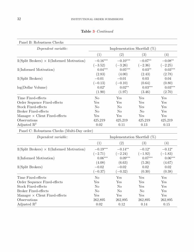
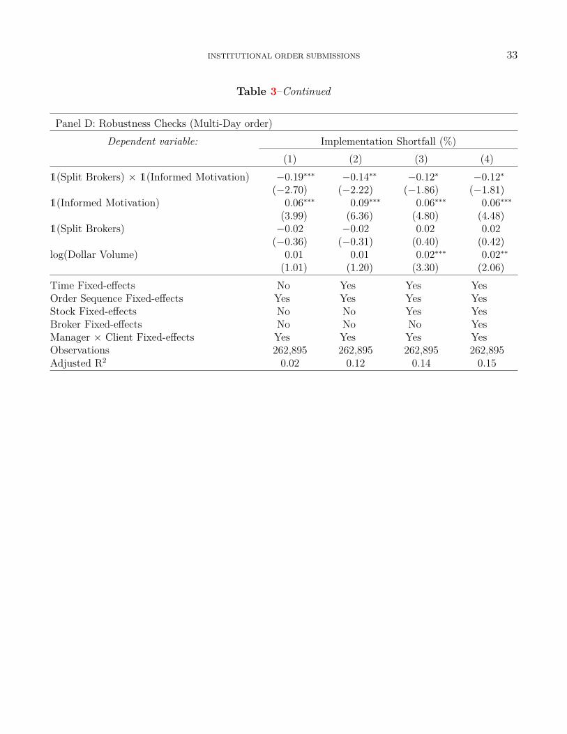
Table 3: Less Implementation Shortfall with splitting order through Brokers

This table examines whether splitting order strategy can reduce trading costs or not. Specifically, we interactSplit Brokersi,k,s,t with 1(Informed Motivatedi,k,s,t) in our specification as follows:

Implementation Shortfalli,k,s,b,t = δ × 1(Informed Motivatedi,k,s,t) × Split Brokersi,k,s,t

+ β × 1(Informed Motivatedi,k,s,t) + λ× Split Brokersi,k,s,t


where i indexes managers, k indexes clients, s index stocks, b indexes brokers, d indexes order-sequence and tindexes trade date. The dependent variable Implementation Shortfalli,k,s,b,t, is the percentage difference between theexecution price and a benchmark price. The independent variable of interest, 1(Informed Motivatedi,k,s,t) denoteswhether the order is driven by informed reason or not and Split Brokersi,k,s,t is one if an institutional investor hiresmore than one broker, zero otherwise. (Daily Basis) In Panel B, we further control for trading dollar volumes. InPanel C and D, we use sub-sample which includes multi-day order. Depending on the specification, the regressionincludes manager × client (fund) fixed effects (αi,k), stock fixed effects (ρs), broker fixed effects (ηb), and timefixed-effects (θt). All regressions include order-sequence fixed effects (γd). Standard errors are clustered by manager× client and the resulting t-statistics are reported in parentheses. Statistical significance at the 10%, 5%, and 1%level is indicated by *, **, and ***, respectively.

Panel A: BaselineDependent variable: Implementation Shortfall (%)

(1) (2) (3) (4)1(Split Brokers) × 1(Informed Motivation) −0.16∗∗∗ −0.11∗∗∗ −0.08∗∗∗ −0.08∗∗

(−3.61) (−3.37) (−2.65) (−2.36)1(Informed Motivation) 0.04∗∗ 0.05∗∗∗ 0.03∗∗∗ 0.03∗∗∗

(2.56) (3.66) (2.80) (2.77)1(Split Brokers) −0.005 −0.004 0.03 0.04

(−0.09) (−0.06) (0.61) (0.79)Time Fixed-effects No Yes Yes YesOrder Sequence Fixed-effects Yes Yes Yes YesStock Fixed-effects No No Yes YesBroker Fixed-effects No No No YesManager × Client Fixed-effects Yes Yes Yes YesObservations 425,219 425,219 425,219 425,219Adjusted R2 0.02 0.11 0.13 0.13


Table 3–Continued

Panel B: Robustness ChecksDependent variable: Implementation Shortfall (%)

(1) (2) (3) (4)1(Split Brokers) × 1(Informed Motivation) −0.16∗∗∗ −0.10∗∗∗ −0.07∗∗ −0.08∗∗

(−3.52) (−3.26) (−2.36) (−2.25)1(Informed Motivation) 0.04∗∗∗ 0.05∗∗∗ 0.03∗∗ 0.03∗∗∗

(2.83) (4.00) (2.43) (2.78)1(Split Brokers) −0.01 −0.01 0.03 0.04

(−0.13) (−0.10) (0.64) (0.80)log(Dollar Volume) 0.02∗ 0.02∗∗ 0.03∗∗∗ 0.03∗∗∗

(1.90) (1.97) (3.46) (2.70)Time Fixed-effects No Yes Yes YesOrder Sequence Fixed-effects Yes Yes Yes YesStock Fixed-effects No No Yes YesBroker Fixed-effects No No No YesManager × Client Fixed-effects Yes Yes Yes YesObservations 425,219 425,219 425,219 425,219Adjusted R2 0.02 0.11 0.13 0.13Panel C: Robustness Checks (Multi-Day order)

Dependent variable: Implementation Shortfall (%)(1) (2) (3) (4)

1(Split Brokers) × 1(Informed Motivation) −0.19∗∗∗ −0.14∗∗ −0.12∗ −0.12∗

(−2.71) (−2.24) (−1.92) (−1.83)1(Informed Motivation) 0.06∗∗∗ 0.09∗∗∗ 0.07∗∗∗ 0.06∗∗∗

(4.08) (6.63) (5.26) (4.67)1(Split Brokers) −0.02 −0.02 0.02 0.02

(−0.37) (−0.32) (0.30) (0.38)Time Fixed-effects No Yes Yes YesOrder Sequence Fixed-effects Yes Yes Yes YesStock Fixed-effects No No Yes YesBroker Fixed-effects No No No YesManager × Client Fixed-effects Yes Yes Yes YesObservations 262,895 262,895 262,895 262,895Adjusted R2 0.02 0.12 0.14 0.15


Table 3–Continued

Panel D: Robustness Checks (Multi-Day order)Dependent variable: Implementation Shortfall (%)

(1) (2) (3) (4)1(Split Brokers) × 1(Informed Motivation) −0.19∗∗∗ −0.14∗∗ −0.12∗ −0.12∗

(−2.70) (−2.22) (−1.86) (−1.81)1(Informed Motivation) 0.06∗∗∗ 0.09∗∗∗ 0.06∗∗∗ 0.06∗∗∗

(3.99) (6.36) (4.80) (4.48)1(Split Brokers) −0.02 −0.02 0.02 0.02

(−0.36) (−0.31) (0.40) (0.42)log(Dollar Volume) 0.01 0.01 0.02∗∗∗ 0.02∗∗

(1.01) (1.20) (3.30) (2.06)Time Fixed-effects No Yes Yes YesOrder Sequence Fixed-effects Yes Yes Yes YesStock Fixed-effects No No Yes YesBroker Fixed-effects No No No YesManager × Client Fixed-effects Yes Yes Yes YesObservations 262,895 262,895 262,895 262,895Adjusted R2 0.02 0.12 0.14 0.15


Table 4: Less Implementation Shortfall: Dynamics over Parent Order

This table examines dynamics of institutional investors’ usage of brokers and shows sending orders tonew brokers can help reduce trading costs. Specifically, we interact 1(Informed Motivatedi,k,s,t) with1(Order Sent to Different Brokeri,k,s,t) in our specification as follows:

Implementation Shortfalli,k,s,b,t = δ × 1(Informed Motivatedi,k,s,t) × 1(Order Sent to Different Brokeri,k,s,t)+ β × 1(Informed Motivatedi,k,s,t) + λ× 1(Order Sent to Different Brokeri,k,s,t)+ αi,k + γd + ρs + ηb + θt + εi,k,s,b,d,t

where i indexes managers, k indexes clients, s index stocks, b indexes brokers, d indexes order-sequence, and tindexes trade date. The dependent variable Implementation Shortfalli,k,s,b,t, is the percentage difference between theexecution price and a benchmark price. The independent variable of interest, 1(Informed Motivatedi,k,s,t) denoteswhether the order is driven by informed reason or not and 1(Order Sent to Different Brokeri,k,s,t) is one if an order issent to different brokers after the first day, zero otherwise. In Panel B, we further control for trading dollar volumes.Depending on the specification, the regression includes manager × client (fund) fixed effects (αi,k), stock fixedeffects (ρs), broker fixed effects (ηb), and time fixed-effects (θt). All regressions include order-sequence fixed effects(γd). Standard errors are clustered by manager × client and the resulting t-statistics are reported in parentheses.Statistical significance at the 10%, 5%, and 1% level is indicated by *, **, and ***, respectively.


(1) (2) (3) (4)1(Order Sent to Different Broker) × 1(Informed Motivation) −0.06∗∗∗ −0.05∗∗ −0.05∗∗∗ −0.05∗∗∗

(−2.89) (−2.46) (−3.36) (−3.31)1(Informed Motivation) 0.01 0.04∗ 0.04∗ 0.03∗

(0.48) (1.92) (1.85) (1.91)1(Order Sent to Different Broker) 0.0003 −0.01 0.003 0.002

(0.04) (−1.01) (0.46) (0.37)Time Fixed-effects No Yes Yes YesOrder Sequence Fixed-effects Yes Yes Yes YesStock Fixed-effects No No Yes YesBroker Fixed-effects No No No YesManager × Client Fixed-effects Yes Yes Yes YesObservations 295,145 295,145 295,145 295,145Adjusted R2 0.02 0.13 0.16 0.16


Table 4–Continued

Panel B: Robustness ChecksDependent variable: Implementation Shortfall (%)

(1) (2) (3) (4)1(Order Sent to Different Broker) × 1(Informed Motivation) −0.06∗∗∗ −0.05∗∗ −0.05∗∗∗ −0.05∗∗∗

(−2.89) (−2.47) (−3.34) (−3.32)1(Informed Motivation) 0.01 0.05∗∗ 0.03∗ 0.03∗

(0.54) (2.07) (1.70) (1.82)1(Order Sent to Different Broker) −0.001 −0.01 0.002 0.003

(−0.13) (−1.27) (0.38) (0.46)log(Dollar Volume) 0.01 0.01 0.02∗∗∗ 0.02∗∗

(1.06) (1.25) (3.88) (2.16)Time Fixed-effects No Yes Yes YesOrder Sequence Fixed-effects Yes Yes Yes YesStock Fixed-effects No No Yes YesBroker Fixed-effects No No No YesManager × Client Fixed-effects Yes Yes Yes YesObservations 295,145 295,145 295,145 295,145Adjusted R2 0.02 0.13 0.16 0.16


Table 5: Camouflage strategies: Evidence from Confidential Holdings

This table examines whether institutional investors submit more order to their brokers who would execute theirinformed order. (submitting camouflage orders to brokers) Specifically, we regress log(Number of Stocks)i,k,b,t on1(Informed Order to Brokeri,k,b,t) in our specification as follows:

log(Number of Stocks)i,k,b,t = β × 1(Informed Order to Brokeri,k,b,t) + αi,k + ηb + θt + εi,k,b,t

where i indexes managers, k indexes clients, b indexes brokers, and t indexes time. The dependent variablelog(Number of Stocks)i,k,b,t, is the number of stocks which are executed through broker at manager-client-tradedate-broker level. The independent variable of interest, 1(Informed Order to Brokeri,k,b,t) is an indicator variable whichis equal to one if a investor submit at least one informed order to a broker, zero otherwise in Panel A. In Panel B,we replace log(Number of Stocks)i,k,b,t with Stock HHIi,k,b,t. Stock HHIi,k,b,t is calculated by squaring the portion ofthe traded aggregate volumes of each stock traded through a broker for investors and then summing the resultingnumbers. We control for the number of shares. Depending on the specification, the regression includes includesmanager × client (fund) fixed effects (αi,k), broker fixed effects (ηb), and time fixed-effects (θt). Standard errors areclustered by manager × client and the resulting t-statistics are reported in parentheses. Statistical significance atthe 10%, 5%, and 1% level is indicated by *, **, and ***, respectively.

Panel A: Baseline

Dependent variable: log(Number of Stocks)(1) (2) (3) (4) (5) (6)

1(Informed Order to Broker) 0.68∗∗∗ 0.72∗∗∗ 0.48∗∗∗ 0.55∗∗∗ 0.57∗∗∗ 0.39∗∗∗

(3.76) (3.68) (9.80) (6.03) (5.90) (19.78)log(volume) 0.21∗∗∗ 0.21∗∗∗ 0.19∗∗∗

(3.88) (3.85) (6.37)Time Fixed-effects No Yes Yes No Yes YesBroker Fixed-effects No No Yes No No YesManager × Client Fixed-effects Yes Yes Yes Yes Yes YesObservations 142,383 142,383 142,383 142,383 142,383 142,383Adjusted R2 0.41 0.42 0.55 0.55 0.56 0.65Panel B: Robustness checks

Dependent variable: Stock HHI(1) (2) (3) (4) (5) (6)

1(Informed Order to Broker) −18.78∗∗∗ −19.80∗∗∗ −13.82∗∗∗ −14.56∗∗∗ −15.16∗∗∗ −10.88∗∗∗

(−4.29) (−4.22) (−12.20) (−8.28) (−8.15) (−25.90)log(volume) −6.67∗∗∗ −6.74∗∗∗ −6.12∗∗∗

(−4.85) (−4.76) (−8.49)Time Fixed-effects No Yes Yes No Yes YesBroker Fixed-effects No No Yes No No YesManager × Client Fixed-effects Yes Yes Yes Yes Yes YesObservations 142,383 142,383 142,383 142,383 142,383 142,383Adjusted R2 0.36 0.37 0.46 0.47 0.48 0.54


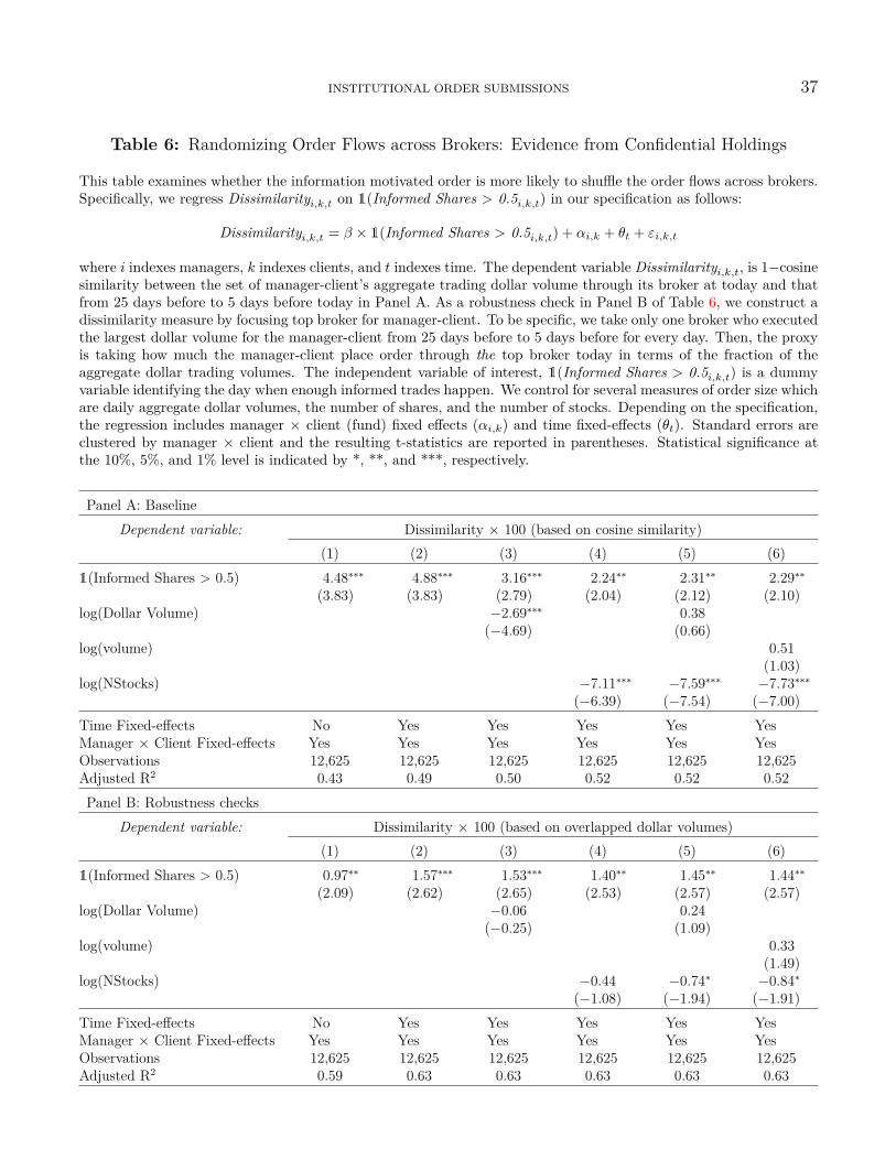
Table 6: Randomizing Order Flows across Brokers: Evidence from Confidential Holdings

This table examines whether the information motivated order is more likely to shuffle the order flows across brokers.Specifically, we regress Dissimilarityi,k,t on 1(Informed Shares > 0.5i,k,t) in our specification as follows:

Dissimilarityi,k,t = β × 1(Informed Shares > 0.5i,k,t) + αi,k + θt + εi,k,t

where i indexes managers, k indexes clients, and t indexes time. The dependent variable Dissimilarityi,k,t, is 1−cosinesimilarity between the set of manager-client’s aggregate trading dollar volume through its broker at today and thatfrom 25 days before to 5 days before today in Panel A. As a robustness check in Panel B of Table 6, we construct adissimilarity measure by focusing top broker for manager-client. To be specific, we take only one broker who executedthe largest dollar volume for the manager-client from 25 days before to 5 days before for every day. Then, the proxyis taking how much the manager-client place order through the top broker today in terms of the fraction of theaggregate dollar trading volumes. The independent variable of interest, 1(Informed Shares > 0.5i,k,t) is a dummyvariable identifying the day when enough informed trades happen. We control for several measures of order size whichare daily aggregate dollar volumes, the number of shares, and the number of stocks. Depending on the specification,the regression includes manager × client (fund) fixed effects (αi,k) and time fixed-effects (θt). Standard errors areclustered by manager × client and the resulting t-statistics are reported in parentheses. Statistical significance atthe 10%, 5%, and 1% level is indicated by *, **, and ***, respectively.

Panel A: BaselineDependent variable: Dissimilarity × 100 (based on cosine similarity)

(1) (2) (3) (4) (5) (6)1(Informed Shares > 0.5) 4.48∗∗∗ 4.88∗∗∗ 3.16∗∗∗ 2.24∗∗ 2.31∗∗ 2.29∗∗

(3.83) (3.83) (2.79) (2.04) (2.12) (2.10)log(Dollar Volume) −2.69∗∗∗ 0.38

(−4.69) (0.66)log(volume) 0.51

(1.03)log(NStocks) −7.11∗∗∗ −7.59∗∗∗ −7.73∗∗∗

(−6.39) (−7.54) (−7.00)Time Fixed-effects No Yes Yes Yes Yes YesManager × Client Fixed-effects Yes Yes Yes Yes Yes YesObservations 12,625 12,625 12,625 12,625 12,625 12,625Adjusted R2 0.43 0.49 0.50 0.52 0.52 0.52Panel B: Robustness checks

Dependent variable: Dissimilarity × 100 (based on overlapped dollar volumes)(1) (2) (3) (4) (5) (6)

1(Informed Shares > 0.5) 0.97∗∗ 1.57∗∗∗ 1.53∗∗∗ 1.40∗∗ 1.45∗∗ 1.44∗∗

(2.09) (2.62) (2.65) (2.53) (2.57) (2.57)log(Dollar Volume) −0.06 0.24

(−0.25) (1.09)log(volume) 0.33

(1.49)log(NStocks) −0.44 −0.74∗ −0.84∗

(−1.08) (−1.94) (−1.91)Time Fixed-effects No Yes Yes Yes Yes YesManager × Client Fixed-effects Yes Yes Yes Yes Yes YesObservations 12,625 12,625 12,625 12,625 12,625 12,625Adjusted R2 0.59 0.63 0.63 0.63 0.63 0.63


Table 6–Continued

Panel C: Robustness checksDependent variable: Dissimilarity × 100 (based on Top Broker)

(1) (2) (3) (4) (5) (6)1(Informed Shares > 0.5) 2.63∗∗ 2.86∗∗ 2.76∗∗ 2.52∗∗ 2.60∗∗ 2.58∗∗

(2.20) (2.06) (2.24) (2.04) (2.13) (2.11)log(Dollar Volume) −0.15 0.42

(−0.21) (0.62)log(volume) 0.55

(1.05)log(NStocks) −0.90 −1.42∗∗ −1.57∗

(−0.82) (−1.98) (−1.77)Time Fixed-effects No Yes Yes Yes Yes YesManager × Client Fixed-effects Yes Yes Yes Yes Yes YesObservations 12,625 12,625 12,625 12,625 12,625 12,625Adjusted R2 0.32 0.38 0.38 0.38 0.38 0.38


Table 7: Randomizing order submission strategies and institutional investors’ performance

This table reports the monthly returns (raw-returns and Daniel et al. (1997) benchmark-adjusted returns) fromJanuary 1999 to November 2009. We sort funds into quantiles based on similarity based on cosine similarity basedon the dollar volume of orders executed by each broker between today’s set of brokers used by a fund and the coreset of brokers used by the same fund (from day t-25 to day t-6). Then we measure the value-weighted buy-and-holdreturn on the stocks bought on each day by each fund, weighted by dollar volume, for the next month (typicallyfrom day t+1 to day t+21). For each quintile, we first average value-weighted returns across funds then use the timeseries average value-weighted returns for statistical inference in the spirit of Fama and MacBeth (1973) and adjustfor serial correlation up to a lag of 20 trading days following Newey and West (1987). The heteroskedasticity robustt-statistics are reported in parentheses. Statistical significance at the 10%, 5%, and 1% level is indicated by *, **,and ***, respectively.

cosine similaritySimilar(Q1) Q2 Q3 Q4 Dis-similar(Q5) D - S

Raw-Return 0.76∗ 0.85∗ 0.93∗ 0.98∗∗ 1.01∗∗ 0.24∗∗∗

(1.69) (1.80) (1.93) (2.06) (2.14) (3.20)DGTW-Adjusted Return 0.29∗∗∗ 0.34∗∗∗ 0.38∗∗∗ 0.45∗∗∗ 0.46∗∗∗ 0.17∗∗∗

(3.81) (4.78) (5.15) (6.07) (6.22) (2.77)


Table 8: Less Implementation Shortfall with more shuffling Order Flows across Brokers

This table examines whether randomization strategy across brokers leads to decrease in trading costs or not. Specif-ically, we interact Dissimilarityi,k,t with 1(Informed Motivatedi,k,s,t) in our specification as follows:

Implementation Shortfalli,k,s,b,t = δ × 1(Informed Motivatedi,k,s,t) × Dissimilarityi,k,t

+ β × 1(Informed Motivatedi,k,s,t) + λ× Dissimilarityi,k,t

+ αi,k + ρs + ηb + θt + εi,k,s,b,t

where i indexes managers, k indexes clients, s index stocks, b indexes brokers, and t indexes time in day. Thedependent variable Implementation Shortfalli,k,s,b,t, is the percentage difference between the execution price anda benchmark price. The independent variable of interest, 1(Informed Motivatedi,k,s,t) denotes whether the orderis driven by informed reason or not and Dissimilarityi,k,t is 1−cosine similarity between the set of manager-client(fund)’s aggregate trading dollar volume through its broker at today and the ones from 25 days before to 5 daysbefore today. In columns (4)-(6), we examine block trades which include a trade’s volume is greater than or equalto 10,000 or its dollar volume is greater than or equal to $200,000. Panel B presents results when controlling forlog(Dollar Volume) or log (volume). In Panel C, we control for trading volume, % in CRSP volume or controlfor trading volume, % in outstanding share. Depending on the specification, the regression includes manager ×client (fund) fixed effects (αi,k), stock fixed effects (ρs), and broker fixed effects (ηb). All regressions include timefixed-effects (θt). Standard errors are clustered by manager × client and the resulting t-statistics are reported inparentheses. Statistical significance at the 10%, 5%, and 1% level is indicated by *, **, and ***, respectively.


(1) (2) (3) (4) (5) (6)Dissimilarity × 1(Informed Motivation) −0.13∗∗∗ −0.12∗∗∗ −0.12∗∗∗ −0.41∗∗∗ −0.36∗∗∗ −0.37∗∗

(−2.86) (−2.58) (−2.58) (−2.86) (−2.64) (−2.55)Dissimilarity 0.04 0.02 0.01 0.08 0.03 0.03

(0.93) (0.39) (0.28) (0.88) (0.33) (0.31)1(Informed Motivation) 0.04∗∗∗ 0.02∗∗∗ 0.02∗∗ 0.06∗∗∗ 0.03∗ 0.03∗

(4.04) (3.11) (2.34) (3.55) (1.92) (1.77)Time Fixed-effects Yes Yes Yes Yes Yes YesStock Fixed-effects No Yes Yes No Yes YesBroker Fixed-effects No No Yes No No YesManager × Client Fixed-effects Yes Yes Yes Yes Yes YesObservations 279,758 279,758 279,758 148,864 148,864 148,864Adjusted R2 0.09 0.11 0.11 0.09 0.11 0.11


Table 8–Continued

Panel B: RobustnessDependent variable: Implementation Shortfall (%)

(1) (2) (3) (4) (5) (6)Dissimilarity × 1(Informed Motivation) −0.13∗∗∗ −0.11∗∗ −0.11∗∗ −0.12∗∗∗ −0.11∗∗ −0.11∗∗

(−2.78) (−2.35) (−2.48) (−2.74) (−2.36) (−2.49)Dissimilarity 0.04 0.01 0.01 0.04 0.01 0.01

(0.89) (0.27) (0.26) (0.88) (0.28) (0.27)1(Informed Motivation) 0.04∗∗∗ 0.02∗∗ 0.02∗∗ 0.04∗∗∗ 0.02∗∗ 0.02∗∗

(3.97) (2.22) (2.02) (3.73) (2.20) (2.00)log(Dollar Volume) 0.01∗∗ 0.02∗∗∗ 0.02∗∗

(1.99) (6.00) (2.47)log(volume) 0.01∗∗∗ 0.02∗∗∗ 0.01∗∗

(2.69) (5.90) (2.29)Time Fixed-effects Yes Yes Yes Yes Yes YesStock Fixed-effects No Yes Yes No Yes YesBroker Fixed-effects No No Yes No No YesManager × Client Fixed-effects Yes Yes Yes Yes Yes YesObservations 279,758 279,758 279,758 279,758 279,758 279,758Adjusted R2 0.09 0.11 0.11 0.09 0.11 0.11Panel C: Robustness

Dependent variable: Implementation Shortfall (%)(1) (2) (3) (4) (5) (6)

Dissimilarity × 1(Informed Motivation) −0.13∗∗∗ −0.14∗∗∗ −0.14∗∗∗ −0.13∗∗∗ −0.12∗∗∗ −0.12∗∗∗

(−2.86) (−3.01) (−3.00) (−2.73) (−2.58) (−2.63)Dissimilarity 0.04 0.02 0.01 0.04 0.02 0.01

(0.95) (0.46) (0.22) (0.91) (0.39) (0.28)1(Informed Motivation) 0.04∗∗∗ 0.04∗∗∗ 0.03∗∗∗ 0.04∗∗∗ 0.02∗∗∗ 0.02∗∗

(3.39) (4.55) (3.66) (3.27) (3.07) (2.52)% in Trading Volume −0.07 −0.63∗∗∗ −0.85∗∗∗

(−0.93) (−4.78) (−4.75)% in Outstanding Share 0.13∗ −0.02 −0.18

(1.67) (−0.20) (−1.33)Time Fixed-effects Yes Yes Yes Yes Yes YesStock Fixed-effects No Yes Yes No Yes YesBroker Fixed-effects No No Yes No No YesManager × Client Fixed-effects Yes Yes Yes Yes Yes YesObservations 279,758 279,758 279,758 279,758 279,758 279,758Adjusted R2 0.09 0.11 0.11 0.09 0.11 0.11


Appendix

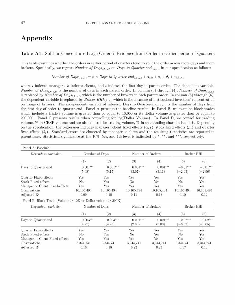
Table A1: Split or Concentrate Large Orders? Evidence from Order in earlier period of Quarters

This table examines whether the orders in earlier period of quarters tend to split the order across more days and morebrokers. Specifically, we regress Number of Daysi,k,s,t on Days to Quarter-endi,k,s,t in our specification as follows:

Number of Daysi,k,s,t = β × Days to Quarter-endi,k,s,t + αi,k + ρs + θt + εi,k,s,t

where i indexes managers, k indexes clients, and t indexes the first day in parent order. The dependent variable,Number of Daysi,k,s,t, is the number of days in each parent order. In column (3) through (4), Number of Daysi,k,s,t

is replaced by Number of Daysi,k,s,t, which is the number of brokers in each parent order. In column (5) through (6),the dependent variable is replaced by Broker HHIi,k,s,t which is the measure of institutional investors’ concentrationon usage of brokers. The independent variable of interest, Days to Quarter-endi,k,s,t is the number of days fromthe first day of order to quarter-end. Panel A presents the baseline results. In Panel B, we examine block tradeswhich include a trade’s volume is greater than or equal to 10,000 or its dollar volume is greater than or equal to200,000. Panel C presents results when controlling for log(Dollar Volume). In Panel D, we control for tradingvolume, % in CRSP volume and we also control for trading volume, % in outstanding share in Panel E. Dependingon the specification, the regression includes manager×client fixed effects (αi,k), stock fixed effects (ρs) and quarterfixed-effects (θt). Standard errors are clustered by manager × client and the resulting t-statistics are reported inparentheses. Statistical significance at the 10%, 5%, and 1% level is indicated by *, **, and ***, respectively.

Panel A: BaselineDependent variable: Number of Days Number of Brokers Broker HHI

(1) (2) (3) (4) (5) (6)Days to Quarter-end 0.001∗∗∗ 0.001∗∗∗ 0.001∗∗∗ 0.001∗∗∗ −0.01∗∗∗ −0.01∗∗∗

(5.08) (5.15) (3.07) (3.11) (−2.95) (−2.96)Quarter Fixed-effects Yes Yes Yes Yes Yes YesStock Fixed-effects No Yes No Yes No YesManager × Client Fixed-effects Yes Yes Yes Yes Yes YesObservations 10,105,494 10,105,494 10,105,494 10,105,494 10,105,494 10,105,494Adjusted R2 0.09 0.10 0.11 0.13 0.10 0.12Panel B: Block Trade (Volume ≥ 10K or Dollar volume ≥ 200K)



(4.27) (4.23) (2.85) (3.08) (−3.32) (−3.65)Quarter Fixed-effects Yes Yes Yes Yes Yes YesStock Fixed-effects No Yes No Yes No YesManager × Client Fixed-effects Yes Yes Yes Yes Yes YesObservations 3,344,741 3,344,741 3,344,741 3,344,741 3,344,741 3,344,741Adjusted R2 0.16 0.18 0.22 0.24 0.17 0.18


Table A1–Continued

Panel C: Robustness checksDependent variable: Number of Days Number of Brokers Broker HHI

(1) (2) (3) (4) (5) (6)Days to Quarter-end 0.001∗∗∗ 0.001∗∗∗ 0.0004∗∗ 0.0004∗∗ −0.01∗∗ −0.01∗∗

(4.32) (4.32) (2.31) (2.30) (−2.22) (−2.20)log(Dollar volume) 0.20∗∗∗ 0.22∗∗∗ 0.16∗∗∗ 0.16∗∗∗ −2.92∗∗∗ −2.88∗∗∗

(8.91) (9.55) (5.61) (6.71) (−6.61) (−8.67)Quarter Fixed-effects Yes Yes Yes Yes Yes YesStock Fixed-effects No Yes No Yes No YesManager × Client Fixed-effects Yes Yes Yes Yes Yes YesObservations 10,105,494 10,105,494 10,105,494 10,105,494 10,105,494 10,105,494Adjusted R2 0.20 0.22 0.25 0.25 0.18 0.19Panel D: Robustness checks



(5.03) (5.11) (3.09) (3.13) (−2.96) (−2.97)Trading volume, % in CRSP volume 0.77 0.90∗∗∗ −1.27∗∗ −0.18∗ 29.12∗∗ 9.05∗∗∗

(1.43) (3.57) (−2.57) (−1.74) (2.12) (2.75)Time Fixed-effects Yes Yes Yes Yes Yes YesStock Fixed-effects No Yes No Yes No YesManager × Client Fixed-effects Yes Yes Yes Yes Yes YesObservations 10,099,641 10,099,641 10,099,641 10,099,641 10,099,641 10,099,641Adjusted R2 0.09 0.10 0.11 0.13 0.10 0.12Panel E: Robustness checks



(5.01) (5.09) (3.09) (3.10) (−2.97) (−2.96)Trading volume, % in Outstanding Share 16.21∗∗∗ 15.53∗∗∗ −8.50∗∗ 6.11∗ 229.12 −29.07

(3.55) (3.57) (−2.06) (1.68) (1.56) (−0.75)Time Fixed-effects Yes Yes Yes Yes Yes YesStock Fixed-effects No Yes No Yes No YesManager × Client Fixed-effects Yes Yes Yes Yes Yes YesObservations 10,105,494 10,105,494 10,105,494 10,105,494 10,105,494 10,105,494Adjusted R2 0.09 0.10 0.11 0.13 0.10 0.12


Table A2: Randomizing Order Flows across Brokers: Evidence from Order in earlier period ofQuarters

This table provides further evidence whether the information motivated order is more likely to shuffle the orderflows across brokers by looking at orders in earlier periods of quarter. Specifically, we regress Dissimilarityi,k,t onDays to Quarter-endi,k,t in our specification as follows:

Dissimilarityi,k,t = β × Days to Quarter-endi,k,t + αi,k + θt + εi,k,t

where i indexes managers, k indexes clients, and t indexes time. The dependent variable Dissimilarityi,k,t, is 1−cosinesimilarity between the set of manager-client’s aggregate trading dollar volume through its broker at today and thatfrom 25 days before to 5 days before today in Panel A. As a robustness check in Panel B of Table A2, we construct adissimilarity measure by focusing top broker for manager-client. To be specific, we take only one broker who executedthe largest dollar volume for the manager-client from 25 days before to 5 days before for every day. Then, the proxy istaking how much the manager-client place order through the top broker today in terms of the fraction of the aggregatedollar trading volumes. The independent variable of interest, Days to Quarter-endi,k,t is the number of days fromthe first day of order to quarter-end. We control for several measures of order size which are daily aggregate dollarvolumes, the number of shares, and the number of stocks. Depending on the specification, the regression includesmanager × client (fund) fixed effects (αi,k), and time fixed-effects (θt). Standard errors are clustered by manager ×client and the resulting t-statistics are reported in parentheses. Statistical significance at the 10%, 5%, and 1% levelis indicated by *, **, and ***, respectively.

Panel A: BaselineDependent variable: Dissimilarity × 100 (based on cosine similarity)

(1) (2) (3) (4) (5) (6)Days to Quarter-end 0.01∗∗∗ 0.01∗∗∗ 0.01∗∗∗ 0.01∗∗∗ 0.01∗∗∗ 0.01∗∗∗

(7.71) (8.44) (11.23) (9.39) (9.88) (9.79)log(Dollar Volume) −2.91∗∗∗ −0.61∗∗∗

(−43.86) (−7.18)log(volume) −0.64∗∗∗

(−7.93)log(NStocks) −6.62∗∗∗ −5.98∗∗∗ −5.95∗∗∗

(−47.59) (−32.36) (−33.67)Time Fixed-effects No Yes Yes Yes Yes YesManager × Client Fixed-effects Yes Yes Yes Yes Yes YesObservations 1,607,092 1,607,092 1,607,092 1,607,092 1,607,092 1,607,092Adjusted R2 0.25 0.25 0.26 0.28 0.28 0.28Panel B: Robustness checks

Dependent variable: Dissimilarity × 100 (based on overlapped dollar volumes)(1) (2) (3) (4) (5) (6)

Days to Quarter-end 0.004∗∗∗ 0.004∗∗∗ 0.004∗∗∗ 0.004∗∗∗ 0.004∗∗∗ 0.004∗∗∗


(−4.33) (−2.78)log(volume) −0.07

(−1.64)log(NStocks) −0.17∗∗∗ −0.03 −0.09

(−3.23) (−0.39) (−1.25)Time Fixed-effects No Yes Yes Yes Yes YesManager × Client Fixed-effects Yes Yes Yes Yes Yes YesObservations 1,607,092 1,607,092 1,607,092 1,607,092 1,607,092 1,607,092Adjusted R2 0.36 0.36 0.36 0.36 0.36 0.36


Table A2–Continued

Panel C: Robustness checksDependent variable: Dissimilarity × 100 (based on Top Broker)

(1) (2) (3) (4) (5) (6)Days to Quarter-end 0.01∗∗∗ 0.01∗∗∗ 0.01∗∗∗ 0.01∗∗∗ 0.01∗∗∗ 0.01∗∗∗


(−8.44) (−4.02)log(volume) −0.23∗∗∗

(−3.04)log(NStocks) −0.72∗∗∗ −0.39∗∗∗ −0.48∗∗∗

(−8.05) (−3.12) (−3.96)Time Fixed-effects No Yes Yes Yes Yes YesManager × Client Fixed-effects Yes Yes Yes Yes Yes YesObservations 1,607,092 1,607,092 1,607,092 1,607,092 1,607,092 1,607,092Adjusted R2 0.18 0.18 0.18 0.18 0.18 0.18

Date post:	03-Feb-2022
Category:	Documents
Upload:	others
View:	0 times
Download:	0 times

Splitting and Shuﬄing: Institutional Trading Motives and ...

Documents