Spray Router with Node Location Dependent Remaining … · and hop-distance-based with...

Spray Router with Node Location DependentRemaining-TTL Message Scheduling in DTNs

著者 Agussalim, Tsuru Masatojournal orpublication title

Journal of Information Processing

volume 24number 4page range 647-659year 2016-07-15URL http://hdl.handle.net/10228/00006296

doi: info:doi/10.2197/ipsjjip.24.647

Journal of Information Processing Vol.24 No.4 647–659 (July 2016)

[DOI: 10.2197/ipsjjip.24.647]

Regular Paper

Spray Router with Node Location DependentRemaining-TTL Message Scheduling in DTNs

Agussalim1,a) Masato Tsuru2,b)

Received: November 16, 2015, Accepted: April 5, 2016

Abstract: Delay and disruption tolerant networks (DTNs) adopt the store-carry-and-forward paradigm. Each nodestores messages in a buffer storage and waits for either an appropriate forwarding opportunity or the message’s expi-ration time, i.e., its time-to-live (TTL). There are two key issues that influence the performance of DTN routing: theforwarding policy that determines whether a message should be forwarded to an encountered node, and the buffer man-agement policy that determines which message should be sent from the queue (i.e., message scheduling) and whichmessage should be dropped when the buffer storage is full. This paper proposes a DTN routing protocol, called spray-and hop-distance-based with remaining-TTL consideration (SNHD-TTL) which integrates three features: (1) binaryspray; (2) hop-distance-based forwarding; and (3) node location dependent remaining-TTL message scheduling. Theaim is to better deliver messages which are highly congested especially in the “island scenario.” We evaluate it bysimulation-based comparison with other popular protocols, namely Epidemic as a baseline and PRoPHETv2 that per-forms well according to our previous study. Our simulation results show that SNHD-TTL is able to outperform otherrouting protocols, significantly reduce overhead, and at the same time, increase the total size of delivered messages.

Keywords: delay tolerant networks, store-carry-forward, routing protocol, message scheduling, island scenario.

1. Introduction

Delay and disruption tolerant networks (DTNs) are designedto perform well in practice, even though there is no end-to-endpath guarantee, to operate effectively over extreme distances suchas those encountered in remote rural areas, space communica-tions or on an interplanetary scale [1]. To deliver a message fromsource node to destination node over challenged and/or oppor-tunistic networks, store-carry-forward-based routing is used [2].With this approach, each relay node (e.g., car and bus) has abuffer storage to store messages while they await an appropriateforwarding opportunity or until the time-to-live (TTL) expires.In DTNs, due to the large uncertainty of relay node mobility andreachability between relay nodes, delivering a single copy of amessage along a single path to the message’s destination is veryunreliable. Therefore, a multi-copy approach is often used tohelp make delivery to the destination more reliable; using this ap-proach, a message is duplicated in the network, and those copiesare delivered (i.e., spread) along multiple paths to the destination.In the last decade, many routing protocols have been proposed forDTNs. Two key issues governing DTN routing are as follows: (1)the forwarding policy that determines whether a message shouldbe forwarded (i.e., copied) to an encountered node and (2) thebuffer management policy that determines which message shouldbe sent from the queue (i.e., message scheduling) and which mes-

1 Graduate School of Computer Science and System Engineering, KyushuInstitute of Technology, Iizuka, Fukuoka 820–8253, Japan

2 Kyushu Institute of Technology, Iizuka, Fukuoka 820–8253, Japana) [email protected]) [email protected]

sage should be dropped when a buffer storage is full. The buffermanagement policy is important for DTN performance especiallyduring congestion where the resources allocated for forwarding(i.e., transmission bandwidth × contact duration) and for storing(i.e., node’s buffer size) are insufficient in relation to the total sizeor density of messages to be transferred on the network.

In our work*1, to understand and improve performance of DTNmessage delivery over multiple separated areas in general, we fo-cus on a specific scenario, i.e., the island scenario, in which asingle stationary source node and a single stationary destinationnode are located on two different islands, (i.e., the large island andthe small island), with two message delivery scenarios: (1) thesource node located in the large island and the destination nodelocated in the small island (LtoS); (2) the source node located inthe small island and the destination node located in the large is-land (StoL). Our work is expected to be easily extended to moregeneral cases in which a limited number of important destinations(e.g., servers, gateways, special terminals, etc.) are stationary andlocated at some areas that are different from the source node’s ar-eas. In our previous study, we compared several popular DTNrouting protocols via simulation and found that there is no singlebest routing algorithm for the island scenario under different con-ditions (e.g., congestion levels) [4]. This motivated us to developa new routing protocol that includes efficient buffer management(involving message scheduling) to increase the performance ofDTNs in the island scenario. Generality is also considered, es-pecially under congested conditions. In the island scenario, thesource and destination nodes are located in separate areas (e.g.,

*1 This paper is an extended version of previously published [3].

c© 2016 Information Processing Society of Japan 647


islands) connected by limited relay nodes (e.g., a ferry). The ferryperiodically shuttles between the two islands and is a bottleneckfor end-to-end delivery because it is the only way to convey mes-sages between the islands. More specifically, the messages leftbehind must wait for the next ferry, which may take a substantialamount of time. Further, since the ferry takes time to make thetrip, some messages may expire during the trip.

Considering the above features, we propose a protocol calledspray-and-hop-distance-based with remaining-TTL consideration(SNHD-TTL), which integrates the following three techniques:(1) binary-spray; (2) hop-distance-based forwarding; and (3)node location dependent remaining-TTL message scheduling. Todeliver each message from the source to the station at the ferryterminal quickly, we use binary spray with an appropriate copylimit. To ensure each message is forwarded between the stationand the ferry in the right direction and to prevent unnecessarymessage transmissions, we use the hop-distance from the desti-nation in the forwarding decision. To give a high priority to mes-sages that will expire if assigned a low priority, we adopt a novelnode location dependent remaining-TTL message scheduling. Toimplement such scheduling, it is assumed that we can estimate theexpected time a message takes to reach its destination depends onits current location.

The TTL, initially set by the source node, is a timer whichlimits the lifetime of a message in the network. When a mes-sage is transmitted from a node to another node, the message’sTTL is updated by subtracting the time for which the messagehas been stored in the sending node (measured by its own clock),and thus it indicates the remaining lifetime of the received mes-sage*2. When the TTL value becomes 0 (i.e., expires), all copiesstored in the network nodes are erased [1].

In addition to this introductory section, the rest of this paperis organized as follows. Section 2 summarizes related study re-garding forwarding and buffer management policies. Section 3presents our proposed routing protocol. Section 4 describes theevaluation scenario. Section 5 describes our simulation results.Finally, the conclusion and directions for future work are de-scribed in Section 6.

2. Related Studies

2.1 ForwardingThe forwarding policy determines which messages should be

forwarded when two nodes encounter one another. If the numberof messages that can be forwarded within a contact duration isenough (i.e., the transmission bandwidth is large enough and/orthe contact duration is long enough) and the number of messagesthat can be stored in a node is sufficient, the simplest, fastest, andmost reliable way to deliver messages to the destination is Epi-demic routing (EP) [5], in which messages are spread to all en-countered nodes of the network to maximize the chance of reach-ing the destination. When two nodes encounter one another, theyexchange a list of message IDs and compare those IDs to deter-mine which message is not already in storage in the other node.

*2 Note that global clock offset synchronization is not required, but a clockskew synchronization is required which is not strictly due to the timegranularity considered in DTN.

Next, those messages are forwarded to the other node; however,its resource consumption increases significantly as the numberof message copies increases. Several studies have focused ontrying to reduce resource consumption [6], [7], [8], [9]. Thesestudies introduced forwarding decisions for controlled flooding,e.g., history-based or utility-based routing. Results of these stud-ies have shown good performance in comparison with simpleflooding. One of the most well-known protocols in this cate-gory is the probabilistic routing protocol using history of encoun-ters and transitivity (PRoPHET) [10]. In another approach, e.g.,SCAR [11], and Spray and Wait [7], a limited number of messagecopies are implemented in each algorithm for message delivery.

Spray and Wait (SNW) routing [7] uses the capabilities ofEP for fast message forwarding and reliable direct transmis-sion, while limiting the number of message copies (i.e., con-trolled flooding). The approach here consists of the following twophases: (1) a spray phase, described in Section 3.1 and (2) a waitphase in which a relay node moves and waits for the opportunityto directly meet up with the destination. Since the wait phase doesnot perform well in some scenarios, including our island scenario,Spray and Focus routing (SNF) [7] has been proposed to addressthis problem; the difference between SNF and SNW is that afterthe spray phase, SNF uses utility-based forwarding to improvedelivery probability. Spray based protocol attracted many re-searchers to improve its performance. The spray protocol was im-proved with probability Choice (SWPC) [15], where the continu-ous encounter time is used to describe the encounter opportunity.Bulut et al. [16] proposed a novel spraying algorithm in whichthe number of message copies in the network depends on the ur-gency of meeting the expected delivery delay for that message.The main objective of this protocol is to give a chance for earlydelivery through small number of copies sprayed in to the net-work. A combination of Spray and Wait [7] and PRoPHET [10]was proposed in [17] which calculates the number of messagecopies to be forwarded based on the performance of the receivernode in the spray phase. In the wait phase, the waiting node usesthe history of encounters and transitivity of transmission. Oneother sophisticated scheme is MaxProp [13], in which the pathcost is computed based on the meeting probability of each hopalong the destination, and the shortest cost path is selected. Notethat our previous work [4] showed that PRoPHETv2 (PV2) [12]outperformed MaxProp in the island scenario. As another ex-ample, You et al. proposed a hop-count-based heuristic routingprotocol for mobile DTNs, which calculates heuristic estimationsbased on hop count information [14]. In particular, they use asliding window mechanism and dynamically updates the averagehop count matrix.

Forwarding a message to the encountered nodes closer to itsdestination (i.e., at a shorter distance) is one of the basic ap-proaches. However, a key issue is how distance to the destinationis defined and estimated (e.g., expected number of hops, expectedtime, expected success probability, etc.). In this paper, whilemore sophisticated schemes have been studied and proposed, weadopt the binary spray protocol, described in Section 3.1, witha simple hop-distance-based forwarding approach, which we de-scribe in Section 3.2.



2.2 Buffer ManagementThere are two kinds of buffer management policies: how to

select messages to be dropped from the buffer storage when thebuffer storage is full, and how to select messages to be sent toa contacted node (i.e., scheduling) within a limited duration ofcontact and transmission bandwidth. Zhang et al. studied the uti-lization of traditional buffer management policies, such as dropfront (DF) and drop tail (DT). They concluded that the DF policyoutperforms DT [20]. Fathima and Wahibanu proposed a buffermanagement scheme with different queues for handling messagesat different priorities. When a buffer is full, a message on a low-priority queue is first dropped to create space for a new mes-sage [18].

Most Forwarded (MOFO) [21] increased the efficiency of mes-sage replication so that routing agents running on nodes keeptrack of the number of times each message is forwarded by anode. A similar idea was explored by Naves et al. [22] whoproposed Less Probable Sprayed (LPS) and Least Recently For-warded (LRF), LPS uses the message delivery probability andestimates the number of replicas already disseminated to decidewhich message to drop. LRF drops the least recently forwardedmessage based on the assumption that unforwarded message overa certain period of time have already reached several next hops.Elwhishi et al. [23] proposed a new message scheduling frame-work for epidemic and two-hop forwarding routing in DTNs. Itincorporates a suite of novel mechanisms for network states es-timation and utility derivation, such that a node can obtain thepriority of each messages to be dropped in case of a full buffer.

Krifa et al. proposed sophisticated buffer management schemescalled global knowledge-based drop and history-based drop [19].These approaches use statistical learning to approximate globalknowledge. By estimating the number of copies of a message,the authors considered the remaining TTL and developed an opti-mal joint scheduling and buffer management scheme based on theestimated necessary parameters using locally collected statisticsby assuming homogeneous and simply modeled mobility. An-other integrated buffer management was proposed [24], that wasbased on statistics and the analysis of the state of the messages.The delivery history of the node and location information wascombined with the relevant information from mutual learning be-tween nodes. Based on the several strategies above, we proposea simple but practical node location dependent remaining-TTLmessage scheduling that utilizes global knowledge about statis-tics obtained from message delivery time in each closed area, i.e.,island, with the remaining TTL value of each message.

3. Spray- and Hop-distance-based withRemaining-TTL Consideration RoutingProtocol (SNHD-TTL)

This section presents the spray-and-hop-distance-based withremaining-TTL consideration (SNHD-TTL) routing protocol,which is illustrated in Fig. 1. This protocol combines the follow-ing three techniques: (1) binary spray for fast and limited mes-sage delivery, with the aim that each message spreads quickly(i.e., with small reduction in the remaining TTL) to a prede-

Fig. 1 Flowchart of SNHD-TTL routing protocol.

fined number of nodes, preventing buffer full conditions; (2) hopdistance to destination-based forwarding to prevent unnecessarymessage transmissions to nodes logically-located further from thedestination, this feature actually prevents messages being for-warded in the opposite (wrong) direction between islands; and(3) node location dependent remaining-TTL message schedulingwhich gives priority to the message queue before forwarding toanother node. This priority divides the message queue depend-ing on node location and remaining TTL. Here, higher priorityis given to messages that have small remaining TTLs that couldreach the destination node. The subsections below provide fur-ther details regarding each component of this protocol.

3.1 Binary SprayThe SNHD-TTL routing protocol employs the “spray phase”

mechanism from binary Spray and Wait [7]. This protocol con-trols the number of messages transmitted by setting up the max-imum number of copies created per messages, which can mini-mize the resource consumption (e.g., bandwidth and buffer stor-age). To initially spread each newly generated message fromits source node to relay nodes while controlling the number ofcopies, binary spray is used in which a copy limit is defined asthe permitted number of copies of a message during the sprayphase. Each message has an initial copy limit L which is gener-ated at its source node. For a message with a copy limit of N (N> 1) stored at node A, whenever node A encounters another nodeB which does not have that message, it is forwarded to node Band the message’s copy limit is changed to half its original value(i.e., �N/2�) at both nodes A and B. For a message with a copylimit of 1 stored at node A, (instead of the “wait phase” in theSpray-and-Wait) SNHD-TTL forwards the message according tothe hop distance-based forwarding mechanism described in thenext subsection.

3.2 Hop Distance Based ForwardingAfter the binary spray phase, (i.e., when the copy limit of mes-



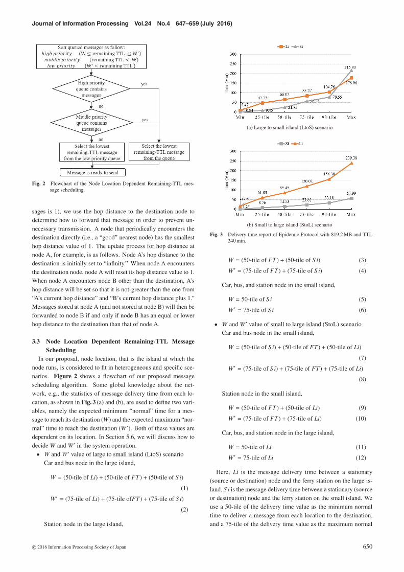
Fig. 2 Flowchart of the Node Location Dependent Remaining-TTL mes-sage scheduling.

sages is 1), we use the hop distance to the destination node todetermine how to forward that message in order to prevent un-necessary transmission. A node that periodically encounters thedestination directly (i.e., a “good” nearest node) has the smallesthop distance value of 1. The update process for hop distance atnode A, for example, is as follows. Node A’s hop distance to thedestination is initially set to “infinity.” When node A encountersthe destination node, node A will reset its hop distance value to 1.When node A encounters node B other than the destination, A’shop distance will be set so that it is not-greater than the one from“A’s current hop distance” and “B’s current hop distance plus 1.”Messages stored at node A (and not stored at node B) will then beforwarded to node B if and only if node B has an equal or lowerhop distance to the destination than that of node A.

3.3 Node Location Dependent Remaining-TTL MessageScheduling

In our proposal, node location, that is the island at which thenode runs, is considered to fit in heterogeneous and specific sce-narios. Figure 2 shows a flowchart of our proposed messagescheduling algorithm. Some global knowledge about the net-work, e.g., the statistics of message delivery time from each lo-cation, as shown in Fig. 3 (a) and (b), are used to define two vari-ables, namely the expected minimum “normal” time for a mes-sage to reach its destination (W) and the expected maximum “nor-mal” time to reach the destination (W ′). Both of these values aredependent on its location. In Section 5.6, we will discuss how todecide W and W ′ in the system operation.• W and W ′ value of large to small island (LtoS) scenario

Car and bus node in the large island,

W = (50-tile of Li) + (50-tile of FT ) + (50-tile of S i)

(1)

W ′ = (75-tile of Li) + (75-tile ofFT ) + (75-tile of S i)

(2)

Station node in the large island,

Fig. 3 Delivery time report of Epidemic Protocol with 819.2 MB and TTL240 min.

W = (50-tile of FT ) + (50-tile of S i) (3)

W ′ = (75-tile of FT ) + (75-tile of S i) (4)

Car, bus, and station node in the small island,

W = 50-tile of S i (5)

W ′ = 75-tile of S i (6)

• W and W ′ value of small to large island (StoL) scenarioCar and bus node in the small island,

W = (50-tile of S i) + (50-tile of FT ) + (50-tile of Li)

(7)

W ′ = (75-tile of S i) + (75-tile of FT ) + (75-tile of Li)

(8)

Station node in the small island,

W = (50-tile of FT ) + (50-tile of Li) (9)

W ′ = (75-tile of FT ) + (75-tile of Li) (10)

Car, bus, and station node in the large island,

W = 50-tile of Li (11)

W ′ = 75-tile of Li (12)

Here, Li is the message delivery time between a stationary(source or destination) node and the ferry station on the large is-land, S i is the message delivery time between a stationary (sourceor destination) node and the ferry station on the small island. Weuse a 50-tile of the delivery time value as the minimum normaltime to deliver a message from each location to the destination,and a 75-tile of the delivery time value as the maximum normal



time. FT is the duration the ferry travels between the station onthe small island and the station on the large island, including thewaiting time at the stations. We define FT as a fixed value, thewait time in the stations is [0, 30] min, and the travel (sailing)time is 15 min. So “the wait time + travel time” is [15, 45]. Then,50-tile is expected to be about 30 min, and 75-tile about 38 min.By combining W and W ′ with remaining-TTL of each message,the message’s priority in the contact duration is determined as fol-lows: the priority is high if W ≤ remaining TTL ≤ W′, middle ifremaining TTL < W and low if W ′ < remaining TTL. Each mes-sage class (queue) is processed in order of its priority from highto low. In each message class, in order of message’s remaining-TTL (lowest remaining-TTL first), the messages that pass the cri-teria of the hop distance-based forwarding phase are forwardedto the contacted node. When the buffer storage is full and a newmessage arrives, a “drop-oldest” policy is used to drop the oldestmessages.

4. Evaluation Scenario

As shown in Fig. 4, the scenario is based on the map-basedmodel and simulated using The Opportunistic Network Environ-

ment (ONE) Simulator [26]. We considered a real-life scenario inwhich two islands, Large island and Small island, are connectedby a ferry between station nodes, with buses and cars as relaynodes and stationary nodes. They can be considered to be sourceand destination nodes on each of the islands. This scenario ismodeled by considering a real situation in Indonesia, and a simi-

Fig. 4 Simulation scenario: large island and small island connected by fer-ryboat.

lar type of scenario can be seen in the literature as well. For ex-ample, Ref. [25] considered island-hopping experiments where astationary node located in three geographically separated groupsare connected by three mobile “traveler nodes.” In our scenario,during the simulated 840 min period of time, ten mobile nodes(e.g., cars and buses) in the large island and six mobile nodesin the small island move on the map’s roads with speeds from5 to 30 km/h, between random location on each island to delivermessages from each destination node according to the messagedelivery scenario. The waiting time of the ferry on each island isabout 30 minutes, and the traveling time (sailing) of the ferryboatbetween two islands is 15 minutes.

We assume the ferry and ferry station nodes on each island asa gateway node with a larger buffer size than the mobile node,which is essential so as not to make the gateway a bottleneck.Since the limitation of the ONE simulator which only supports2,000 MB of maximum buffer storage size, we used the follow-ing in the scenario: 1:10 comparison ratio for the buffer size, eachmobile node has a 200 MB buffer, then the gateway node has a2,000 MB buffer. Later in Section 5.8 we also evaluate our pro-posed method with the increased buffer size ratio of 1:2 since it isclose to reality.

The origin of the messages depend on the message deliveryscenario. Messages are generated in a stationary source node lo-cated on an island and destined to a stationary destination nodeon the other island. In the LtoS scenario, the source is located onthe large island, and in the StoL scenario, the source is located onthe small island. The source node generates messages with size0.4 MB, and various total sizes [204.8 MB, 409.6 MB, 819.2 MB,1,638.4 MB, and 3,276.8 MB] within 480 min. To change the to-tal size, we control the average time-interval of message gener-ation. The message time-to-live (TTL) of 240 and 480 min areused for each simulation scenario. A larger value of TTL willhave more chances for a message to reach its destination, whilemore messages stored in the network node’s for long periods oftime will potentially increase the consumption of resources (e.g.,bandwidth and buffer space). To adapt the comparison ratio ofthe buffer size, we decreased the WiFi link interface with a trans-mission data rate of 1 Mbps and an omni-directional transmission

Table 1 Simulation parameters.

Parameter Value

Simulation time 840 min

Node buffer size Car and Bus = 200 MB

Station A and B, Ferry = 2,000 MB

Interface transmit speed and range 1 Mbps and 25 m

Message lifetime (TTL) 240 and 480 min

Node speed Bus = 5–20 km/h

Car = 10–30 km/h

Total size (amount) of originally- 204.8 MB, 409.6 MB, 819.2 MB

generated messages 1,638.4 MB, 3,276.8 MB

Message created duration 480 min from the beginning

Message size 0.4 MB

Warm up time 30 min



range of 25 m as scaling. To evaluate our proposal with a dif-ferent buffer-size and WiFi-rate relation, later in Section 5.8, weincrease the transmission rate and transmission range as consid-ered in Refs. [27] and [28] with the increased buffer size ratio of1:2. In order to get meaningful comparison results, the simulationscenario was executed 10 times using different movement seeds.Each figure shows the average value calculated from these results.

As discussed previously, SNHD-TTL employs binary spraywith a parameter of L and the remaining-TTL consideration withparameters of W and W ′. As default values, we used an L of3, and W and W ′ are obtained from statistics derived from mes-sage delivery time of EP with 819.2 MB of the total size of gen-erated messages. Later in Sections 5.5 and 5.6, we examine anddiscuss the impact of these parameters on SNHD-TTL’s perfor-mance. Table 1 summarizes the simulation parameters used inour evaluations.

5. Simulation Results

The performance of the SNHD-TTL routing protocol is com-pared through simulation against two popular DTN routing pro-tocols, EP and PV2, plus two comparative routing protocols, EP-TTL (the EP protocol integrated with node location dependentremaining-TTL message scheduling), and SNHD (our proposedprotocol without node location dependent remaining-TTL mes-sage scheduling). We used three performance metrics: the to-tal size of delivered messages, overhead ratio, and average la-tency. The aim of our simulation study is to understand the im-pact of combining the considered techniques (i.e., binary spray,hop distance-based forwarding, and node location dependentremaining-TTL message scheduling) on improving the perfor-mance of DTN routing. We also evaluate the impact of increasingthe number of nodes in each island, varying the number of copiesL in the spray phase of SNHD-TTL, and sensitivity of W and W′

values as obtained from the statistics of the message delivery timeon the performance of SNHD-TTL.

5.1 The Total Size of Delivered MessagesThe total size of delivered messages is defined as the size of

the message multiplied by the number of messages successfullydelivered to the destination during the simulation. Figure 5 (a)and (b) show the total size of delivered messages with a TTL of240 min under the LtoS and StoL message delivery scenarios. Asthe total generated size (i.e., the x-axis in the figures) increases,the network becomes congestion. In non- or weakly congestedstates, the performance of each protocol is similar. On the otherhand, in congested states, a significant performance differenceamong protocols is seen. For the TTL 240 min performance ofSNHD-TTL both message delivery scenarios are almost the sameand perform the best across all protocols. In the LtoS scenario,EP-TTL and EP achieved lower performance, while in the StoLscenario, EP achieved better performance than EP-TTL, PV2, andSNHD for the 1,638.4 MB and 3,276.8 MB cases.

Figure 6 (a) and (b) show the total size of delivered messageswith a TTL of 480 min, which indicate performance among allof protocols depends on message delivery scenarios. Comparedwith Fig. 5 (a) and (b), in both LtoS and StoL scenarios, the per-

Fig. 5 The total size of delivered messages with TTL 240 min.

Fig. 6 The total size of delivered messages with TTL 480 min.

formance advantage of SNHD-TTL to other protocols is muchgreater.

In summary, except in cases of non- or weakly congestedstates, SNHD-TTL clearly outperformed other protocols irrespec-tive of the delivery scenarios (StoL or LtoS) and TTL (240 min or480 min).

For buffer management, we compared EP with EP-TTL andSNHD with SNHD-TTL. For EP-TTL, we found that this methoddid not significantly improve performance as compared with EP,



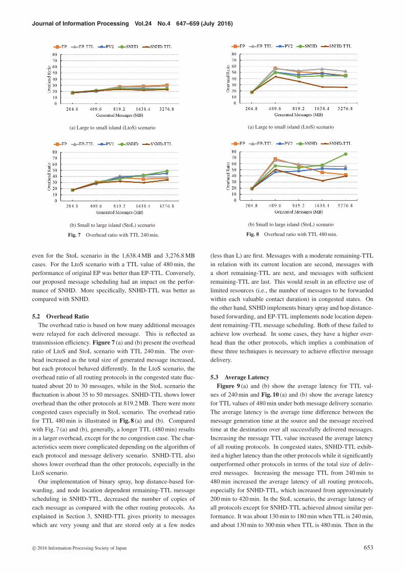
Fig. 7 Overhead ratio with TTL 240 min.

even for the StoL scenario in the 1,638.4 MB and 3,276.8 MBcases. For the LtoS scenario with a TTL value of 480 min, theperformance of original EP was better than EP-TTL. Conversely,our proposed message scheduling had an impact on the perfor-mance of SNHD. More specifically, SNHD-TTL was better ascompared with SNHD.

5.2 Overhead RatioThe overhead ratio is based on how many additional messages

were relayed for each delivered message. This is reflected astransmission efficiency. Figure 7 (a) and (b) present the overheadratio of LtoS and StoL scenario with TTL 240 min. The over-head increased as the total size of generated message increased,but each protocol behaved differently. In the LtoS scenario, theoverhead ratio of all routing protocols in the congested state fluc-tuated about 20 to 30 messages, while in the StoL scenario thefluctuation is about 35 to 50 messages. SNHD-TTL shows loweroverhead than the other protocols at 819.2 MB. There were morecongested cases especially in StoL scenario. The overhead ratiofor TTL 480 min is illustrated in Fig. 8 (a) and (b). Comparedwith Fig. 7 (a) and (b), generally, a longer TTL (480 min) resultsin a larger overhead, except for the no congestion case. The char-acteristics seem more complicated depending on the algorithm ofeach protocol and message delivery scenario. SNHD-TTL alsoshows lower overhead than the other protocols, especially in theLtoS scenario.

Our implementation of binary spray, hop distance-based for-warding, and node location dependent remaining-TTL messagescheduling in SNHD-TTL, decreased the number of copies ofeach message as compared with the other routing protocols. Asexplained in Section 3, SNHD-TTL gives priority to messageswhich are very young and that are stored only at a few nodes

Fig. 8 Overhead ratio with TTL 480 min.

(less than L) are first. Messages with a moderate remaining-TTLin relation with its current location are second, messages witha short remaining-TTL are next, and messages with sufficientremaining-TTL are last. This would result in an effective use oflimited resources (i.e., the number of messages to be forwardedwithin each valuable contact duration) in congested states. Onthe other hand, SNHD implements binary spray and hop distance-based forwarding, and EP-TTL implements node location depen-dent remaining-TTL message scheduling. Both of these failed toachieve low overhead. In some cases, they have a higher over-head than the other protocols, which implies a combination ofthese three techniques is necessary to achieve effective messagedelivery.

5.3 Average LatencyFigure 9 (a) and (b) show the average latency for TTL val-

ues of 240 min and Fig. 10 (a) and (b) show the average latencyfor TTL values of 480 min under both message delivery scenario.The average latency is the average time difference between themessage generation time at the source and the message receivedtime at the destination over all successfully delivered messages.Increasing the message TTL value increased the average latencyof all routing protocols. In congested states, SNHD-TTL exhib-ited a higher latency than the other protocols while it significantlyoutperformed other protocols in terms of the total size of deliv-ered messages. Increasing the message TTL from 240 min to480 min increased the average latency of all routing protocols,especially for SNHD-TTL, which increased from approximately200 min to 420 min. In the StoL scenario, the average latency ofall protocols except for SNHD-TTL achieved almost similar per-formance. It was about 130 min to 180 min when TTL is 240 min,and about 130 min to 300 min when TTL is 480 min. Then in the



Fig. 9 Average latency with TTL 240 min.

Fig. 10 Average latency with TTL 480 min.

LtoS scenario, the difference among protocols varies, dependingon the size of the generated messages. For example, EP has alower latency in the 409.6 Mb case and then becomes higher thanthe other protocols except for SNHD-TTL in the 819.2 MB and1,638.4 MB cases when TTL is 240 min.

5.4 Impact of Increasing Number of Nodes in Each Islandon The Total Size of Delivered Messages

In this evaluation, we increased the number of nodes on both

Fig. 11 Impact of increasing the number of nodes on the total size of deliv-ered messages.

islands. In the large island, the number of nodes is increased from10 (6 cars and 4 buses) to 15 (9 cars and 6 buses), then in the smallisland it is increased from 5 (3 cars and 2 buses) to 9 (6 cars and3 buses). Figure 11 (a) and (b) show the total size of deliveredmessages as the number of nodes increases. In general, increas-ing the number of nodes will increase the performance comparedwith the default number of nodes. Increasing the number of nodesincreased the number of messages that can be stored in the bufferstorage on the network as well as the number of messages thatcan be exchanged by contacts between nodes. This decreased thedelay time of messages to reach the destination node. As shownin Fig. 12 (a) and (b), the average latency of 28 nodes is lowerthan 19 nodes in the LtoS and StoL scenarios.

5.5 Impact of Varying the Number of copies (L) on The To-tal Size of Delivered Messages

As shown in Fig. 13 (a) and (b), we evaluated the impact ofthe number of generated message copies (L) in the spray phaseon the performance of SNHD-TTL in terms of the total size ofdelivered messages. In the LtoS scenario, varying L had a signifi-cant impact in cases where the size of generated messages totaled819.2 MB or more. Note that the total size of delivered messagesfor all L values was almost the same for the cases from 204.8 MBto 409.6 MB, because the network capacity was large enough forall messages. When a congested state occurred, the larger num-ber of copies caused a decrease in performance, because as L

increased, the number of message transmissions also increased.Then in the StoL scenario, the total size of delivered messageswith different L values achieved similar performance except inthe 3,276.8 MB case, where small L values achieved better per-formance than the other values. Figure 14 (a) and (b) show theimpact of the L values on the average latency. In the LtoS sce-



Fig. 12 Impact of increasing the number of nodes on the average latency.

Fig. 13 L impact on the total size of delivered messages.

nario the number of L values significantly affected the averagelatency. Increasing the L values will decrease the average latencywhile in the StoL scenario the average latency is almost the sameas all of the L values.

5.6 Impact of W and W′ on SNHD-TTL’s PerformanceNode location dependent remaining-TTL message scheduling

used the statistics of delivery time in order to determine W andW ′ values. In the previous subsections, we used statistics from

Fig. 14 L impact on the average latency.

Table 2 W and W ′ value from EP.

Msg. Gen. Size Value Li Node Station Li Si Node

204.8 MBW 69.36 37.01 7.01

W′ 89.47 47.51 9.51

409.6 MBW 81.10 37.46 7.46

W′ 107.79 48.33 10.33

819.2 MBW 120.87 54.85 24.85

W′ 179.80 94.54 56.54

1,638.4 MBW 175.81 105.19 75.19

W′ 275.17 171.37 133.37

3,276.8 MBW 184.80 110.89 80.89

W′ 309.12 210.42 172.42

the delivery time of EP with 819.2 MB of the total size of gen-erated messages to determine W and W ′ to serve as the baseline.We assume they can be roughly estimated beforehand from in-formation obtained by some means, e.g., simulations or real fieldnode measurements.

Table 2 provides W and W ′ values according to the total size ofgenerated messages which are calculated from the delivery timereport in Fig. 3 using the formula in Section 3.3. “Msg. Gen.Size” column contains information about the total size of the orig-inally generated messages. The “Li Node” column contains W

and W ′ values for the mobile node on the large island. The “Sta-tion Li” column contains W and W ′ values for the station node onthe large island. The “Si Node” column contains W and W′ valuesfor the station node and the mobile node on the small island.

For calculating the LtoS scenario, from Fig. 3 we get the 75-tile and 50-tile values for the large island as (Li) = 85.27 min and66.02 min respectively. Then for the small island, we have (S i) =56.54 min and 24.85 min respectively. Then for the ferry travel-ing time (FT ) we used fixed values of 38 min for the 75-tile, and30 min for the 50-tile which are determined based on the trav-



Table 3 W and W ′ value from SNHDTTL using W and W ′ value in casewith 819.2 MB case in Table 2.


204.8 MBW 70.66 38.24 8.24

W′ 93.08 51.24 13.24

409.6 MBW 74.93 37.19 7.19

W′ 101.70 48.20 10.20

819.2 MBW 104.13 38.79 8.79

W′ 152.44 52.59 14.59

1,638.4 MBW 140.56 39.77 9.77

W′ 181.62 53.53 15.53

3,276.8 MBW 148.53 43.29 13.29

W′ 195.86 60.22 22.22

Table 4 W and W ′ value from SNHDTTL using W and W ′ value in Table 3.


204.8 MBW 91.23 39.66 9.66

W′ 129 47.52 9.52

409.6 MBW 104.08 38.13 8.13

W′ 155.88 49.81 11.81

819.2 MBW 109.05 42.82 12.82

W′ 260.20 159.67 121.67

1,638.4 MBW 131.55 47.42 17.42

W′ 362.63 228.25 190.25

3,276.8 MBW 153.38 46.12 16.12

W′ 229.22 77.80 39.80

eling time and waiting time of the ferry on each island. Fromeach formula in Section 3.3, we get W and W′ of EP 819.2 MB asfollows:• Li Node, using Eqs. (1) and (2)

W = 66.02 + 30 + 24.85 = 120.87

W ′ = 85.27 + 38 + 56.54 = 179.80

• Station Li, using Eqs. (3) and (4)

W = 30 + 24.85 = 54.85

W ′ = 38 + 56.54 = 94.54

• Si Node, using Eqs. (5) and (6)

W = 24.85

W ′ = 56.54

In this subsection, we show the impact of W and W′ values onthe message delivery performance, and discuss how to find andcalibrate appropriate W and W ′ values. As shown in Table 3, newW and W ′ values are determined from the statistics of the messagedelivery time of SNHD-TTL as obtained by simulation using theW and W ′ values for the case of 819.2 MB from Table 2. Then, asshown in Table 4, different new W and W′ values are determinedfrom the statistics of the message delivery time of SNHD-TTLas obtained by the simulation using previously determined W andW ′ values for each message generated size case from Table 3. Forexample, we simulate SNHD-TTL with the 204.8 MB messagegenerated size using W and W ′ values for the case of 204.8 MBin Table 3. We compare the total size of delivered messages ofSNHD-TTL using different W and W ′ values. In Fig. 15 (a) and

Fig. 15 W and W ′ impact on the total size of delivered messages.

(b), EP409, EP819, and EP1638 mean SNHD-TTL using W andW ′ values obtained from the message delivery time statistics ofEP in each of 409.6 MB, 819.6 MB and 1,638.4 MB cases in Ta-ble 2, respectively. Those cases are intended to represent a staticSNHD-TTL that uses the same W and W ′, irrespective of mes-sage generated sizes, i.e., congestion states. Note that EP819is equivalent to the default SHND-TTL as evaluated in previoussubsections. SNHDTTL(1) and SNHDTTL(2) mean the SNHD-TTL using the W and W ′ values obtained from SNHD-TTL ineach corresponding message generated size case as shown in Ta-bles 3 and 4, respectively. Those cases are intended to representan adaptive SNHD-TTL that uses the different W and W′ in re-sponse to message generated sizes, (i.e., congestion states) andthus we call them SNHDTTL-adaptive.

In the LtoS scenario, as shown in Fig. 15 (a), if the mes-sage generated size is small, (i.e., 204.8 MB and 409.6 MBcases) the performance is not affected by W and W′. However,when the message generated size is large, EP1638 achieved thelowest performance. EP819 achieved lower performance thanEP409, SNHDTTL(1), and SNHDTTL(2) in the 638.4 MB and3,276.8 MB cases. SNHDTTL(1) and SNHDTTL(2) achieved thebest performance. In the StoL scenario as shown in Fig. 15 (b),when the message generated size is small, (i.e., 204.8 MB,409.6 MB, and 819.2 MB cases) the performance is not af-fected by W and W ′. EP409 achieved the lowest performancewhen the message generated size is large, (i.e., 1,638.4 MB and3,276.8 MB cases). SNHDTTL(1) showed slightly lower perfor-mance than EP819, EP1638 and SNHDTTL(2) in the 1,638.4 MBcase.

These results indicate that the use of the same W and W′ in-dependent of message generated sizes may cause performancedegradation in some cases and it is difficult to determine a sin-



Fig. 16 The size of island impact on the total size of delivered messages.

gle best pair of W and W ′ (i.e., EP409, EP819, and EP1638). Incontrast, SNHDTTL(1) and SNHDTTL(2), that is SNHDTTL-adaptive, showed similar and stable performance. In addi-tion, in some cases (StoL scenario in the 1,638.4 MB and3,276.8 MB cases), SNHDTTL(2) achieved better performancethan SNHDTTL(1). Therefore, an adaptive calibration of W andW ′ by updating them during operation should be considered. Thestatistics of message delivery time is required, to determine W

and W ′ for each location. Sharing this information among nodesin an online manner is also needed. This could be possible byrecording the history of TTL updates in all or some messages,monitoring them at stationary landmark nodes (the ferry stationsand the destination in our scenario), and distributing this infor-mation, for example.

5.7 Impact of Increasing the Size of IslandThis evaluation shows the impact of increasing the size of the

island on the performance of all routing protocols. We increasedthe island size by using two larger maps that are enlarged by 2xand 3x from the original map as shown in Fig. 4, respectively, andset the scenario parameters by 480 min of TTL value, 819.2 MBof the total size of generated messages and increasing the numberof nodes from 19 nodes in the original scenario to 28 nodes. Wedetermined the W and W ′ values according to each island sizeusing message delivery reports of EP 819.2 MB. Figure 16 (a)and (b) show the impact of increasing the size of the island on thetotal size of delivered messages. In general, as the size of the is-land increases, the performance of all routing protocols decreasesand, at the same time, the advantage of our proposed SNHDTTLprotocol using a single (W,W ′) also decreases even though it stillworks with a better or almost equal performance to other proto-cols. These results suggest, in larger island scenarios, we need to

Fig. 17 The size of island impact on the average latency.

consider not only refining the selection of (W,W′) but introducinganother refinement such as area partitioning.

Increasing the size of the island also affects the average latencyas shown in Fig. 17 (a) and (b). When the island size increased 3xthe average latency of all protocols also increased and becomesimilar. These results indicate the difference between SNHDTTLand the other protocols will become smaller for larger island sce-narios.

5.8 Impact of Increasing Buffer Size and WiFi TransmitRate and Range

In Section 4, we discussed about our simulation scenario. Dueto the limitation of the maximum buffer size in the ONE simula-tor, we used a comparison ratio 1:10 for the buffer size of nodes(i.e., 2,000 MB for the gateway nodes, and 200 MB for mobilenodes), with a WiFi transmission rate and range of 1 Mbps and25 m, respectively. In this section we discuss about the impact ofincreasing the buffer size ratio and WiFi transmit rate and range.We decreased the comparison ratio of buffer size from 1:10 to 1:2(i.e., gateways nodes is 2,000 MB and mobile nodes is 1,000 MB),and increased the WiFi transmission rate and range to 4.5 Mbpsand 30 m, as considered in Refs. [27], and [28]. We also omit-ted 204.8 MB and added 6,553.6 MB as the largest of the totalsize of generated messages. Since a congestion state of this newscenario occurred when the total size of generated messages was3,276.8 MB, the W and W′ values are determined by message de-livery report of EP 3,276.8 MB.

Increasing the buffer size and WiFi transmit rate and rangeaffected the performance of all routing protocols as shown inFigs. 18 and 19. Increasing the buffer size of mobile nodes willincrease the total capacity of the network. A congestion statestarted when the total size of generated message is 3,276.8 MB



Fig. 18 Buffer size and WiFi transmit rate and range increasing impact onthe total size of delivered messages TTL 240 min.

Fig. 19 Buffer size and WiFi transmit rate and range increasing impact onthe total size of delivered messages TTL 480 min.

while in the original scenario, it is 819.2 MB. Increasing the WiFitransmit rate and range increased the number of messages thatcan be transferred in a single moment of contact. Figure 18 (a)and (b) show the performance of all protocols in TTL 240 min.They achieved almost the same performance from 409.6 MBto 1,638.4 MB then in 3,276.8 MB and 6,553.6 MB, SNHDTTLachieved better performance than the other protocols.

Then for TTL 480 min (Fig. 19 (a) and (b)), the performance

of all routing protocols increase compared with TTL 240 min. Inboth LtoS and StoL scenarios, SNHDTTL achieved better per-formance compared to the other protocols when the total sizeof generated messages is 3,276.8 MB or more. Unfortunately inStoL scenario (Fig. 19 (b)), although the total size of generatedmessages increases twice to 6,553.6 MB the performance of allprotocols except EP-TTL decreased.

6. Conclusions and Future Work

In this paper, we have proposed the spray-and-hop-distance-based with remaining-TTL consideration (SNHD-TTL). Thisrouting protocol integrated three techniques: binary spray,hop distance-based forwarding, and node location dependentremaining-TTL message scheduling, to fit on the island scenariowith two message delivery scenarios (i.e., large island to smallisland, and small island to large island). Global knowledge aboutstatistics obtained from message delivery time is used for TTL-based message scheduling. Applying these combined techniques,we observed that SNHD-TTL outperformed the other evaluatedrouting protocols. Results also showed that in congested states, asmaller number of message copies was better in the spray phase.Increasing the number of nodes resulted in better performancefor all routing protocols due to the capacity of the network (i.e.,buffer storage) being increased. It is also suggested that static W

and W ′ values independent of congestion states are not very effec-tive, although appropriate static values showed to work to someextent in our scenarios. In our future work, we aim to develop away to dynamically learn and estimate W and W′ in practical sys-tem operation. For scenarios with multiple sources and destina-tions, we may need to introduce more sophisticated hop distancebased forwarding. In addition, we will also consider introducingthe network coding techniques as suggested in Ref. [25].

Acknowledgments This work is supported by the Direc-torate General of Resources for Science, Technology and HigherEducation of Indonesia Government and partly supported byJSPS KAKENHI (25330108).

References

[1] Vasilakos, A.V., Zhang, Y. and Spyropoulos, T. (Eds.): Delay TolerantNetworks: Protocols and Applications, CRC press (2011).

[2] Jain, S., Fall, K. and Patra, R.: Routing in a Delay Tolerant Network,ACM, Vol.34, No.4, pp.145–158 (2004).

[3] Agussalim and Tsuru, M.: Node location dependent remaining-TTLmessage scheduling in DTNs, Proc. IEEE Asia Pacific Conference onWireless and Mobile (APWiMob 2015), pp.108–113 (2015).

[4] Agussalim and Tsuru, M.: Comparison of DTN routing protocols inrealistic scenarios, Proc. IEEE Intelligent Networking and Collabora-tive Systems (INCoS ’14), pp.400–405 (2014).

[5] Vahdat, S. and Becker, D.: Epidemic routing for partially-connectedad hoc networks, Technical Report CS-200006 Duke University(2000).

[6] Matsuda, T. and Takine, T.: (p, q)-epidemic routing for sparsely pop-ulated mobile ad hoc networks, IEEE Journal on Selected Areas inCommunications, Vol.26, No.5, pp.783–793 (2008).

[7] Spyropoulos, T., Psounis, K. and Raghavendra, C.S.: Efficient routingin intermittently connected mobile networks: The multiple-copy case,IEEE/ACM Trans. Networking, Vol.16, No.1, pp.77–90 (2008).

[8] Balasubramanian, A., Levine, B.N. and Venkataramani, A.: DTNrouting as a resource allocation problem, ACM SIGCOMM ComputerCommunication Review, Vol.37, No.4, pp.373–384 (2007).

[9] Nelson, S.C., Bakht, M., Kravets, R. and Harris, A.F.: Encounter-based routing in DTNs, ACM SIGMOBILE Mobile Computing Com-munication Review, Vol.13, No.1, pp.56–59 (2009).



[10] Lindgren, A., Doria, A. and Schelen, O.: Probabilistic routing in inter-mittently connected networks, ACM SIGMOBILE Mobile Computingand Communications Review, Vol.7, No.3, pp.19–20 (2003).

[11] Mascolo, C. and Musolesi, M.: SCAR: Context-aware adaptive rout-ing in delay tolerant mobile sensor networks, Proc. 2006 Interna-tional Conference on Wireless Communications and Mobile Comput-ing, pp.533–538, ACM (2006).

[12] Grasic, S., Davies, E., Lindgren, A. and Doria, A.: The evolution ofa DTN routing protocol- PRoPHETv2, Proc. 6th ACM Workshop onChallenged Networks, pp.27–30 (2011).

[13] Burgess, J., Gallagher, B., Jensen, D. and Levine, B.N.: MaxProp:routing for vehicle-based disruption-tolerant networks, Proc. INFO-COM 25th IEEE, Vol.6, pp.1–11 (2006).

[14] You, L., Li, J., Wei, C., Xu, J. and Hu, L.: A hop count based heuris-tic routing protocol for mobile delay tolerant networks, The ScientificWorld Journal, Vol.2014, Hindawi Publishing Corporation (2014).

[15] Pan, D., Lin, M., Chen, L. and Sun, J.: An improved spray and waitwith probability choice routing for opportunistic networks, Journal ofNetworks, Vol.7, No.9, pp.1486–1492 (2012).

[16] Bulut, E., Wang, Z. and Szymanski, B.K.: Time dependent messagespraying for routing in intermittently connected networks, IEEE Proc.Global Telecommunications Conference (GLOBECOM 2008), pp.1–6(2008).

[17] Mehto, A. and Chawla, M.: Modified different neighbour history sprayand wait using PROPHET in delay tolerant network, Proc. Interna-tional Journal of Computer Application, Foundation of Computer Sci-ence, Vol.86, No.18 (2014).

[18] Fathima, G. and Wahidabanu, R.S.D.: A new queueing policy for de-lay tolerant network, International Journal of Computer Applications,Citeseer, Vol.1, No.20, pp.56–59 (2010).

[19] Krifa, A., Barakat, C. and Spyropoulus, T.: Message drop and schedul-ing in DTNs: Theory and practice, IEEE Trans. Mobile Computing,Vol.11, No.9, pp.1470–1483 (2012).

[20] Zhang, X., Neglia, G., Kurose, J. and Towsley, D.: Performance mod-eling of epidemic routing, Journal of Computer Networks, Vol.51,No.10, pp.2867–2891, Elsevier (2007).

[21] Lindgren, A. and Phanse, K.S.: Evaluating of queueing policies andforwarding strategies for routing in intermittently connected networks,Proc. 1st International Conference on Communication System Soft-ware and Middleware, Comsware 2006, pp.1–10 (2006).

[22] Naves, J.F., Moraes, I.M. and Albuquerque, C.: LPS and LRF: Ef-ficient buffer management policies for delay and disruption tolerantnetworks, Proc. 37th Annual IEEE Conference on Local ComputerNetworks, pp.368–375 (2012).

[23] Elwishi, A., Ho, P.H., Naik, K. and Shihada, B.: A novel mes-sage scheduling framework for delay tolerant networks routing, IEEETrans. Parallel and Distributed Systems, Vol.24, No.5, pp.871–880(2013).

[24] Pan, D., Ruan, Z., Zhou, N., Liu, X. and Song, Z.: A comprehensive-integrated buffer management strategy for opportunistic networks,EURASIP Journal on Wireless Communications and Networking,Vol.2013, No.1, pp.1–10, Springer (2013).

[25] Hennessy, A., Gladd, A. and Walker, B.: Nullspace-based stoppingconditions for network-coded transmission in DTNs. Proc. 7th ACMInternational Workshop on Challenged Networks, pp.51–56 (2012).

[26] Keranen, A.: Opportunistic network environment simulator, SpecialAssignment report, Helsinki University of Technology, Department ofCommunications and Networking (2008).

[27] Keranen, A. and Ott, J.: Increasing reality for DTN protocol simula-tions, Helsinki University of Technology, Technology Report (2007).

[28] Wellens, M., Westhphal, B. and Mahonen, P.: Performance evalua-tion of IEEE 802.11-based WLANs in vehicular scenarios, IEEE 65thVehicular Technology Conference, pp.1167–1171 (2007).

Agussalim received B.Ed. in electricalengineering education from State Univer-sity of Makassar, Indonesia (UNM) in2007, M.E. in electrical engineering witha major in informatics engineering fromHasanuddin University, Indonesia (UN-HAS) in 2012. He is currently a doctoralstudent in the Department of Information

System, Graduate School of Computer Science and System Engi-neering, Kyushu Institute of Technology, Japan. His research in-terests include delay, disruption, disconnection tolerant networks(DTNs) and multihop wireless network. He is a student memberof IEICE.

Masato Tsuru received B.E. and M.E.degrees from Kyoto University, Japan in1983 and 1985, respectively, and then re-ceived his D.E. degree from Kyushu In-stitute of Technology, Japan in 2002. Heworked at Oki Electric Industry Co., Ltd.,Nagasaki University, and Japan TelecomInformation Service Co., Ltd. In 2003, he

moved to the Department of Computer Science and Electronics,Kyushu Institute of Technology as an Associate Professor, andhas been a Professor in the same department since April 2006.His research interests include performance measurement, model-ing, and management of computer communication networks. Heis a member of ACM, IEEE, IEICE, IPSJ, and JSSST.


Date post:	17-Jun-2018
Category:	Documents
Upload:	nguyenquynh
View:	215 times
Download:	0 times

Spray Router with Node Location Dependent Remaining … · and hop-distance-based with...

Documents