Spreadsheet physics: Examples in meteorology and planetary science Rhett Herman Citation: American Journal of Physics 77, 1124 (2009); doi: 10.1119/1.3230033 View online: http://dx.doi.org/10.1119/1.3230033 View Table of Contents: http://scitation.aip.org/content/aapt/journal/ajp/77/12?ver=pdfcov Published by the American Association of Physics Teachers Articles you may be interested in Moons and Planets: An Introduction to Planetary Science Phys. Teach. 52, 319 (2014); 10.1119/1.4872435 Linear least squares, the spreadsheet, and Filip Am. J. Phys. 75, 619 (2007); 10.1119/1.2721585 User-Defined Scroll Bars in Spreadsheets Phys. Teach. 42, 166 (2004); 10.1119/1.1664384 A Last Chance for Getting It Right: Addressing Alternative Conceptions in the Physical Sciences Phys. Teach. 41, 36 (2003); 10.1119/1.1533963 Spreadsheet waves Phys. Teach. 37, 14 (1999); 10.1119/1.880141 This article is copyrighted as indicated in the article. Reuse of AAPT content is subject to the terms at: http://scitation.aip.org/termsconditions. Downloaded to IP: 192.122.237.11 On: Mon, 28 Apr 2014 23:50:15
Transcript
Spreadsheet physics: Examples in meteorology and planetary scienceRhett Herman
Citation: American Journal of Physics 77, 1124 (2009); doi: 10.1119/1.3230033 View online: http://dx.doi.org/10.1119/1.3230033 View Table of Contents: http://scitation.aip.org/content/aapt/journal/ajp/77/12?ver=pdfcov Published by the American Association of Physics Teachers Articles you may be interested in Moons and Planets: An Introduction to Planetary Science Phys. Teach. 52, 319 (2014); 10.1119/1.4872435 Linear least squares, the spreadsheet, and Filip Am. J. Phys. 75, 619 (2007); 10.1119/1.2721585 User-Defined Scroll Bars in Spreadsheets Phys. Teach. 42, 166 (2004); 10.1119/1.1664384 A Last Chance for Getting It Right: Addressing Alternative Conceptions in the Physical Sciences Phys. Teach. 41, 36 (2003); 10.1119/1.1533963 Spreadsheet waves Phys. Teach. 37, 14 (1999); 10.1119/1.880141
This article is copyrighted as indicated in the article. Reuse of AAPT content is subject to the terms at: http://scitation.aip.org/termsconditions. Downloaded to IP:
Spreadsheets offer a way to balance the need for obtainingsimple numerical solutions to the equations of physics with-out going too deeply into programming methods1 and areespecially useful if students do not have any programmingexperience. Spreadsheets have been used to obtain numericalsolutions for a number of physical situations, includingLaplace’s equation,2–4 Ampere’s law,5 and Faraday’s law.6
These solutions involved two-dimensional situations andused a number of circular references and the iterative capa-bilities of spreadsheets to handle such self-references. Otherapplications have been to linear and angular kinematicequations7,8 and to quantum systems.1 MacDonald examinedthe errors that inevitably arise in such numerical solutions.9
Spreadsheets lend themselves to simple programmingwhen first-order differential equations are written as finitedifference equations. When differential equations are writtenas finite difference equations, they may be evolved byspreadsheets in one of two ways. The simpler way may beused when all quantities depend on one parameter, that is,when they arise from ordinary differential equations, for ex-ample, the time. The initial values for the position, velocity,and time may be specified in one row of a spreadsheet. Forthe case of one-dimensional motion with constant accelera-tion, the acceleration may be specified in a single cell andcalled by the equations through an absolute cell reference.The next row of the spreadsheet contains the equations forthe values for the position, velocity, and time after one timestep �t. This row refers back to the initial values in the firstrow. The second row is then copied in subsequent rows toevolve the equations until the desired final time is reached.Note that the default is for the spreadsheet to calculate allvalues in the copied cells. In this way the user can see theevolution of the variables in each row of the spreadsheet.
Another method of evolving difference equations is re-quired when they arise from partial differential equations. Inthis case spreadsheets do not immediately perform the calcu-lations but rather wait for the user to start the iterations, forexample, by pressing a certain control key. Then the spread-sheet performs only the number of iterations set by the pro-grammer. This method allows cells to refer back to them-selves �a circular reference�. The limited number of iterationsmeans that the spreadsheet does not attempt to calculate end-less loops.
Consider the evolution of the equation xf =xi+�x. Instead
of having xf and xi in row upon row down the spreadsheet,
1124 Am. J. Phys. 77 �12�, December 2009 http://aapt.org/ajp
icle is copyrighted as indicated in the article. Reuse of AAPT content is sub
192.122.237.11 On: Mon,
the equation may be evolved within a single cell. Let cell A2be the one that evolves with time. With �x=1, the code thatgoes in A2 would be =A2+1. This code would normallycreate a circular reference. However the iterations functionallows this input and does not immediately try to calculatethis circular reference in a never-ending loop. Suppose thatthe initial value for A2 after entering this code is one. Thespreadsheet will only calculate the value for A2 when a cer-tain control key is pressed �F9 in EXCEL� and will only iteratethe calculation the number of times specified when the itera-tions function is enabled. For example, if the maximum it-erations are set to 100, then pressing the control key threetimes yields 301 for cell A2.
An example of this method for solving coupleddifferential/difference equations may be observed by settingcell A2 to =B2+3 and cell B2 to =A2+1. Pressing the con-trol key three times will yield 1201 and 1204 for A2 and B2,respectively, assuming the number of iterations is set for 100.
This paper describes examples of these two types ofspreadsheet programming. The example from planetary sci-ence uses the first of the two methods to model the density,pressure, temperature, mass, and gravitational acceleration ofa planet. Initial conditions at r=0 are specified and equationsof state for these variables are evolved outward from thatpoint. The second spreadsheet method is illustrated by mod-eling the atmosphere of Earth. Modeling Earth’s atmosphereis difficult because it requires many parameters, is highlynonlinear, and has much data to accommodate.
There are a number of spreadsheet programs available,both free and commercial. I used Microsoft EXCEL forthis work. For information on enabling the iterations andscroll bars in Excel see �www.radford.edu/~rherman/spreadsheets/�.
II. PLANETARY MODELS
Building a model for an incompressible solid or liquidplanet requires starting from r=0 and evolving the equationsto the surface. Defining the surface of the planet is straight-forward for a solid planet. The pressure decreases monotoni-cally and thus the surface is the radius r for whichP=0.
Building the planet starts from the equation of hydrostatic
ject to the terms at: http://scitation.aip.org/termsconditions. Downloaded to IP:
28 Apr 2014 23:50:15
This art
dP
dr= − �g , �1�
where � is the density and g is the gravitational acceleration.Equation �1� may be approximated as the difference equation
Pf = Pi − �ig�rf − ri� . �2�
For a solid or liquid planet the form of � may be assumed tobe
� f = �i�1 − ��� , �3�
where the parameter ���1. Equation �3� can be derivedfrom the relation
d� = − ��dr , �4�
which has the solution
� f = �ie−��r, �5�
where �r�rf −ri. For ��r�1 � f ��i�1−��r�. Because ��ris dimensionless, it is useful to define �����r, which leadsto Eq. �3�. The form of Eq. �3� was initially chosen for itssimplicity but yields results for a planet with a final size andmass close to the values for Earth.
The overall mass interior to a given radius is computed byadding the mass of each shell of thickness �r starting fromr=0. The mass in each shell is obtained by rewriting thedifferential equation dm=�dV as the difference equation
mf = mi + �dV = mi + �i4�ri2�rf − ri� . �6�
The mass of each shell �i4�ri2�rf −ri� is added to that of the
prior shell mi to obtain the total.The gravitational acceleration is calculated using
gf =Gmf
rf2 , �7�
where mf is the total mass interior to the current radius r asgiven by Eq. �6�. The step size �r in rf =ri+�r must be smallcompared to any value for r, which is accomplished by set-ting
rf = ri�1 + �r� , �8�
where the parameter �r�1.For an ideal gas planet the equations are integrated starting
from r=0 and evolved until the surface is reached. The lo-cation of the surface is arbitrary because the pressure will notbecome equal to zero. The surface may be chosen as theradius where the pressure is sufficiently small compared tosome reasonable value such as the initial pressure.
The main difference between the solid and ideal gas plan-etary models is in the equation of state for the density. If weassume ideal gas behavior throughout, the density � is givenby
� =m
V=
m
NkT/P= m
N P
kT, �9�
where k=1.38�10−23 J /K and �m /N� is the mass per par-ticle of the planet. The temperature is chosen in the samemanner as that of the density in the solid/liquid planet. Thus
Tf = Ti�1 − �T� , �10�
where the parameter �T�1.
1125 Am. J. Phys., Vol. 77, No. 12, December 2009
icle is copyrighted as indicated in the article. Reuse of AAPT content is sub
192.122.237.11 On: Mon,
The spreadsheet has columns for the radius r, pressure P,density �, cumulative mass m, and gravitational accelerationg. In addition, two cells are used as absolute references forthe radius increase and temperature decrease factors, �� and�T, respectively.
III. TWO-LAYER ATMOSPHERIC MODEL
The complex relation between the data and the modelsmeans the relative contributions of energy inputs and outputsare continually being refined. A good introduction to the ba-sics of modeling the atmosphere is given in Refs. 10 and 11.For simplicity, Earth’s atmosphere may be modeled as asingle-layer atmosphere overlying a single-layer surface,both with a uniform composition. This model follows closelythe model described by Boeker and van Grondelle12 and as-sumes that each boundary has an input that is reflected, trans-mitted, and absorbed to varying degrees. The model is finetuned by adjusting the parameters for the degree of eachinput/output process. The model accounts for the release ofenergy by each layer by radiation.
This model assumes the area of the flat single-layer atmo-sphere is equal to the total surface area of Earth, Atotal=4�R2, where R is the radius of Earth. The magnitude of thesolar flux at Earth’s distance from the Sun is Ftotal�S=1370 W /m2. The symbol F will be used for flux, withunits of W /m2.
The input S encounters only that part of Earth facing theSun, which has an area �R2. This flux must be distributedover the total surface area of Earth’s atmosphere, which is4�R2. Thus the effective solar input is Feffective= �1 /4�S. Thefraction of this input reflected by the atmosphere is given byFr,a=aa�1 /4�S, where aa is the albedo of the atmosphere,which has a typical value aa�0.30 but may be changed toexplore the consequences of other values.13
Part of the input is transmitted through the atmosphere tothe surface and is given by Ft,a= ta�1 /4�S. The transmissioncoefficient has a typical value ta�0.50.13 The remaining fluxis absorbed by the atmosphere: Fabs,a= �1−aa− ta��1 /4�S.These and other equations discussed here are shown inFig. 1.
The flux transmitted by the atmosphere proceeds to thesurface, where part is reflected and the remainder is ab-sorbed. The flux reflected by the surface is Fr,s=asFt,a=asta�1 /4�S. Although the radiation is reflected, transmitted,and absorbed by the atmosphere again, for simplicity weassume that the radiation is fully absorbed by the atmo-
Fig. 1. Two-layer atmospheric model showing the energy flow. “Space” isabove the atmosphere. Both the surface and the atmosphere are of finitethickness �after Fig. 3.2 in Ref. 12�.
sphere. This assumption is consistent with the greenhouse
1125Rhett Herman
ject to the terms at: http://scitation.aip.org/termsconditions. Downloaded to IP:
28 Apr 2014 23:50:15
This art
mechanism whereby a fraction of the light with multiplewavelengths reaching the surface is reradiated at infraredwavelengths. The infrared radiation is then trapped by green-house gases such as water vapor and CO2.13
The assumption of 100% absorption of the infrared rera-diation shows students how simplifying assumptions aremade in modeling. In fact some fraction of this IR radiationis not trapped but is transmitted through the atmosphere intospace. This process of reflection-transmission-absorptioncould be repeated endlessly, albeit with decreasing magni-tude with each step. The present model will not consider thisrepeated process.
The flux absorbed by the surface is Fabs,s= �1−as�Ft,a= �1−as�ta�1 /4�S. This flux is the remainder from the originalradiation transmitted through the atmosphere reaching thesurface.
Because the atmosphere and the surface have energy in-puts and thus nonzero temperatures, they will radiate thatenergy away. The atmosphere will radiate both into space aswell as back to the surface, each with a magnitude of Frad,a=ea�Ta
4, where ea is the emissivity of the atmosphere, �=5.67�10−8 W /m2 K4 and Ta is the temperature of the at-mosphere. The radiation from the top of the atmosphere goesinto space. The radiation from the bottom of the atmosphereis assumed to be completely absorbed by the surface.
The surface will radiate with a magnitude of Frad,s=es�Ts
4, where es is the emissivity of the surface. The radia-tion will then be reflected, transmitted, and absorbed by theatmosphere. These terms are given by Fref,s−a=aa�es�Ts
4,Ftrans,s−a= ta�es�Ts
4, and Fabs,s−a= �1−aa�− ta��es�Ts4, respec-
tively. The flux reflected by the atmosphere is assumed to becompletely absorbed by the surface.
The final factor is the flux conducted between the surfaceand the atmosphere. This flux is given by Fcond=��Ts−Ta�,where � is the thermal conductivity with units of W /m2 K.The sign of Fcond will show the direction of the flux.
The goal is to find the final equilibrium temperatures ofthe surface and the atmosphere given the inputs and outputswe have described. The evolution of the temperatures is ac-complished through the first-order approximation
Tf � Ti + dT
dt�t , �11�
where �t is the time step. The rate dT /dt is obtained fromQ=mc�T, where Q is the inexact differential for heattransferred to/from the layer, m is the mass, and c is thespecific heat capacity of the layer. This equation may berewritten as Q /dt�mcdT /dt and
dT
dt=
1
mc
Q
dt. �12�
The mass m may be rewritten using m=�V=�Az, where � isthe density, A is the horizontal area, and z is the thickness ofthe layer. The difference equation for the temperature evolu-tion of the layer is now
Tf � Ti +1
c�z
Q
Adt�t . �13�
The term Q /Adt is the flux transferred to/from the layer.
For the atmosphere this term is
1126 Am. J. Phys., Vol. 77, No. 12, December 2009
icle is copyrighted as indicated in the article. Reuse of AAPT content is sub
192.122.237.11 On: Mon,
Q
Adt= �1 − aa − ta�1
4S + asta1
4S + �1 − aa� − ta��es�Ts
4
− 2ea�Ta4 + ��Ts − Ta� , �14�
where the parameters to be chosen by the programmer are aa,ta, as, aa�, ta�, es, ea, and �. For the surface
Q
Adt= �1 − as�ta1
4S − �1 − aa��es�Ts
4
+ ea�Ta4 − ��Ts − Ta� . �15�
The parameters to be chosen are as, ta, aa�, es, ea, and �.In equilibrium the rates in Eqs. �14� and �15� are both
equal to zero. With two unknowns and for fixed values of theparameters, solving for the equilibrium values for Ts and Tabecomes an exercise in algebra.
Substituting Eqs. �14� and �15� into Eq. �13� leads to twocoupled partial differential equations for the temperatureevolution for the surface and the atmosphere. These may bewritten as difference equations in the manner of Sec. II. Aspreadsheet may then be programmed with these equations,and the use may see the temperatures change as the modelcomes to equilibrium.
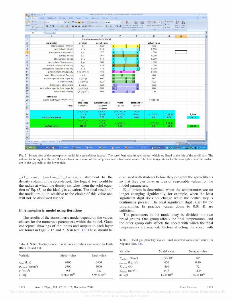
The list of parameters to be set by the programmer is long.It would be tedious to continually type in values for theseeach time they are changed. It is useful to set these using thescroll bar tools available in spreadsheets. A screen shot of thespreadsheet used for the current work is shown in Fig. 2.
IV. RESULTS
A. Planetary models
For the solid planetary model the parameters were��=4.8�10−4, �r=0.01, Pcentral=1.70�10−11 N /m2, and�central=1.13�104 kg /m3. This choice led the pressure tochange sign at r�6400 km, which is the location of thesurface of the model planet. The final values for this modeland those for Earth are listed in Table I.
The ideal gas planetary model doesn’t yield results that areas good because of the presence of solid cores in real gasgiant planets.15 The two planetary models we have discussedmay be combined by using an equation such as Eq. �3� tomodel a solid core that gives way to the ideal gas equation ofstate at some larger radius. Such a combined model has itsown difficulties such as discontinuities in the values for thepressure and density at the outer boundary of the solid coreand will not be discussed here.
Because the pressure never goes to zero in the ideal gasmodel, the choice of the surface is arbitrary. We chose as theradius r�24,700 km, the approximate radius of Neptune.15
The parameters chosen for this model were Pcentral=5.80�1011 N /m2, �central=5.61�10104 kg /m3, Tcentral=3000 K, �T=1.1�1010−3, and �r=0.01. Neptune has anatmosphere of 80% H2 and 20% He,15 and thus the mass perparticle was chosen to be 4.007�1010−27 kg. The values forthis model and those for Neptune are listed in Table II. InRef. 15 the surface of Neptune is considered to be the radiuswhere P�105 N /m2.
The computed values compare only marginally to the ac-cepted values for the surface of Neptune. Adding a solid coreto the gas giant would add another layer of realism but wouldadd more complexity to the model. This may be accom-
plished by adding an IF(logical_test, value-
1126Rhett Herman
ject to the terms at: http://scitation.aip.org/termsconditions. Downloaded to IP:
28 Apr 2014 23:50:15
This art
_if_true, [value_if_false]) statement to thedensity column in the spreadsheet. The logical_test would bethe radius at which the density switches from the solid equa-tion of Eq. �3� to the ideal gas equation. The final results ofthe model are quite sensitive to the choice of this value andwill not be discussed further.
B. Atmospheric model using iterations
The results of the atmospheric model depend on the valueschosen for the numerous parameters within the model. Goodconceptual drawings of the inputs and outputs to each layerare found in Figs. 2.15 and 2.16 in Ref. 13. These should be
Table I. Solid planetary model: Final modeled values and values for Earth�Refs. 14 and 15�.
Fig. 2. Screen shot of the atmospheric model in a spreadsheet �EXCEL�. Thecolumn to the right of the scroll bars allows conversion of the integer valueare in the two cells at the lower right.
1127 Am. J. Phys., Vol. 77, No. 12, December 2009
icle is copyrighted as indicated in the article. Reuse of AAPT content is sub
192.122.237.11 On: Mon,
discussed with students before they program the spreadsheetsso that they can have an idea of reasonable values for themodel parameters.
Equilibrium is determined when the temperatures are nolonger changing significantly, for example, when the leastsignificant digit does not change while the control key iscontinually pressed. The least significant digit is set by theprogrammer. In practice values down to 0.01 K aresufficient.
The parameters in the model may be divided into twobroad groups. One group affects the final temperatures, andthe other group only affects the speed with which the finaltemperatures are reached. Factors affecting the speed with
Table II. Ideal gas planetary model: Final modeled values and values forNeptune �Ref. 15�.
l bars take integer values, which are listed to the left of the scroll bars. Theractional values. The final temperatures for the atmosphere and the surface
scrols to f
1127Rhett Herman
ject to the terms at: http://scitation.aip.org/termsconditions. Downloaded to IP:
28 Apr 2014 23:50:15
This art
which equilibrium is reached include the density �, thicknessz, and specific heat c for each layer. These factors determinethe total heat capacity C for each layer by the relation C=mc=�Vc=�Azc.
The other group of factors influences the final tempera-tures by determining the amount of energy going into and outof each layer. These include the reflection and transmissioncoefficients, the emissivities, and the conductivity betweenthe two layers. The parameters that influence the finaltemperatures are S, aa, ta, as, aa�, ta�, es, ea, and the surface/atmosphere conductivity �. Typical values for theseparameters are S=1370 W /m2, aa�0.30,ta�0.52, as�0.11, aa��0.30, ta��0.06, es�0.90, ea�0.90,and �=2.7 W /m2 K.12,13
Suppose that the time step is �t=5000 s=1.58�10−4 years and each press of the control key is 1000 itera-tions. One press of the control key causes a time passage of0.158 years, with final temperatures of Tatmosphere=31.30 Kand Tsurface=1.11 K after those 1000 iterations. After 6 yearsthe temperature of the atmosphere is 76.77 K and that of thesurface is 46.37 K. The surface temperature lags behind thatof the atmosphere until over 25 years have passed. After 25years the sign of the heat conducted between the surface andthe atmosphere changes, showing students the “real time”effects of the final term in both Eqs. �14� and �15�.
After �70 years the change in the temperatures is in thesecond decimal place, and by �90 years the temperatureshave become Tatmosphere=228.16 K and Tsurface=269.85 K.The modeled temperature for the atmosphere is significantlylower than the current value of 288 K for the atmosphere justabove Earth’s surface.13 Students should be encouraged toadjust the parameters of their models so that the modeledTatmosphere becomes closer to 288 K.
The difference in the surface and the atmospheric tempera-ture illustrates the greenhouse effect provided by Earth’s at-mosphere. Assuming no atmosphere and blackbody behavior,the average temperature of Earth would be 255 K.13 Studentsmay adjust the parameters accordingly and see the modelevolve to this approximate state.
Students may also see how the temperatures in this modelreact to their changes. For example, changing the solar fluxto S=1390 W /m2 and letting two years pass changes thefinal temperatures to Tatmosphere=228.46 K and Tsurface=270.05 K. This direct increase in the final temperatureswith the increase in solar inputs is in accordance with moresophisticated models.16
For S=1370 W /m2 and atmospheric albedo equal to 0.31,we find Tatmosphere=227.53 K and Tsurface=269.75 K after 2years. These temperature reductions are again consistent withthe increased atmospheric albedo, reflecting more of the in-put back into space. Several other factors may be studied.For example, as the concentration of CO2 increases, thetransmission coefficient ta� should decrease, indicating agreater trapping of the reradiated infrared radiation from thesurface.
V. EXPERIENCE IN THE CLASSROOM
I have used these models in two intermediate-levelcourses, Meteorology and Solar System Astronomy. Thecourses do not assume a rigorous background in upper-level
physics classes. The prerequisites for each course include 1
1128 Am. J. Phys., Vol. 77, No. 12, December 2009
icle is copyrighted as indicated in the article. Reuse of AAPT content is sub
192.122.237.11 On: Mon,
year of either algebra-based or calculus-based introductoryphysics. Thus these models are accessible to nonphysicsmajors.
In both classes I wanted students to gain an appreciationfor the process of numerical modeling and how these modelshave contributed to what is in their textbooks. For example,when my students are told the value for the radius of a gasgiant outside of our solar system, I want them to know thatthis estimate is based on the few examples in our solar sys-tem along with numerical modeling. When they hear that therising concentration of CO2 in our atmosphere could lead toa given temperature change after a certain time, I want themto know this relation between CO2 concentration and tem-perature has been carefully modeled.
Even these simplistic numerical models are difficult. I donot expect students to complete these models in just a fewdays. Rather I introduce pieces of these models throughoutthe semester in hopes that their final models are fairly so-phisticated given their backgrounds.
Students have told me that these models have been diffi-cult and that they have learned to appreciate the difficultiesthat “real” numerical modeling must entail. A not inconse-quential amount of my time right before the final models aredue is spent in troubleshooting their programs. They come toappreciate that one typing error, one exponent in error, orsome other little factor can throw off the entire model.
I have found that the students who do the iterative atmo-spheric model often continue to adjust their parameters evenafter the course is finished. One student even added in somehigher order terms to the first-order terms I have listed here.He remarked how those higher order terms made a small butnonzero contribution to the overall model. The possibilitiesfor students to make their own adjustments in the spread-sheet models discussed here are numerous.
ACKNOWLEDGMENT
The author would like to thank the referees for helpfulsuggestions in revising this paper.
a�Electronic mail: [email protected] V. Kinderman, “A computing laboratory for introductory quantummechanics,” Am. J. Phys. 58�6�, 568–573 �1990�.
2T. T. Crow, “Solutions to Laplace’s equation using spreadsheets on apersonal computer,” Am. J. Phys. 55�9�, 817–823 �1987�.
3Francis X. Hart, “Validating spreadsheet solutions to Laplace’s equation,”Am. J. Phys. 57�11�, 1027–1034 �1989�.
4Salvador Gil, Martin Eduardo Saleta, and Dina Tobia, “Experimentalstudy of the Neumann and Dirichlet boundary conditions in two-dimensional electrostatic problems,” Am. J. Phys. 70�12�, 1208–1213�2002�.
5Francis X. Hart, “Spreadsheet solutions for Ampere’s law problems withirregularly shaped conductors,” Am. J. Phys. 65�6�, 565–567 �1997�.
6Francis X. Hart and Kenneth W. Wood, “Eddy current distributions: Theircalculation with a spreadsheet and their measurement with a dual dipoleantenna probe,” Am. J. Phys. 59�5�, 461–467 �1991�.
7C. W. Misner, Patrick J. Cooney, and Jesusa V. Kinderman, SpreadsheetPhysics �Addison-Wesley, Reading, MA, 1991�.
8P. W. Laws, “A unit on oscillations, determinism and chaos for introduc-tory physics students,” Am. J. Phys. 72�4�, 446–452 �2004�.
9William M. MacDonald, “Discretization and truncation errors in a nu-merical solution of Laplace’s equation,” Am. J. Phys. 62�2�, 169–173�1994�.
10J. R. Barker and M. H. Ross, “An introduction to global warming,” Am.J. Phys. 67�12�, 1216–1226 �1999�.
11 R. S. Knox, “Physics aspects of the greenhouse effect and global warm-
ing,” Am. J. Phys. 67�12�, 1227–1238 �1999�.
1128Rhett Herman
ject to the terms at: http://scitation.aip.org/termsconditions. Downloaded to IP:
28 Apr 2014 23:50:15
This art
12E. Boeker and R. van Grondelle, Environmental Physics, 2nd ed. �Wiley,New York, 1999�.
13Arnold Ahrens, Meteorology Today: An Introduction to Weather, Climate,and the Environment, 7th ed. �Brooks-Cole, Pacific Grove, CA, 2003�.
14H. R. Burger, A. F. Sheehan, and C. H. Jones, Introduction to Applied
1129 Am. J. Phys., Vol. 77, No. 12, December 2009
icle is copyrighted as indicated in the article. Reuse of AAPT content is sub
192.122.237.11 On: Mon,
Geophysics �Norton, New York, 2006�.15I. De Pater and J. J. Lissauer, Planetary Sciences �Cambridge U.P., Cam-
bridge, 2001�.16N. Scafetta and B. West, “Is climate sensitive to solar variability,” Phys.
Today 61�3�, 50–51 �2008�.
Crown of Cups Battery. In 1800 Alessandro Volta �1745–1827� described the Crown of Cups in a letter to Sir JosephBanks, the President of the Royal Society. It consisted of a series of glasses, often arranged in a circle, containingacidulated or salt water, and connected by metal straps dipping into the liquid. These straps consisted of a ribbon ofone metal �say copper� soldered to the end of a ribbon of another metal �say zinc�. The name of the apparatus arisesfrom its circular shape. This example is in the Garland Collection of Classical Physics Apparatus at VanderbiltUniversity. �Photograph and Notes by Thomas B. Greenslade, Jr., Kenyon College�
1129Rhett Herman
ject to the terms at: http://scitation.aip.org/termsconditions. Downloaded to IP: