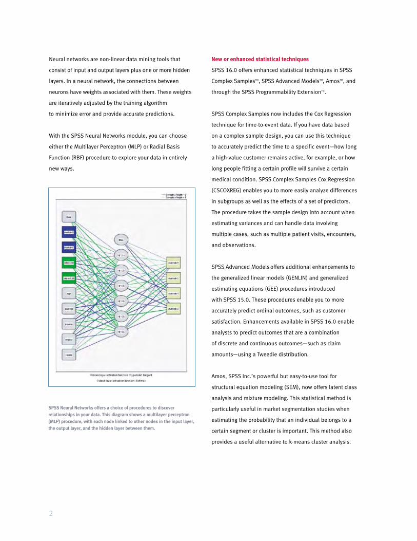
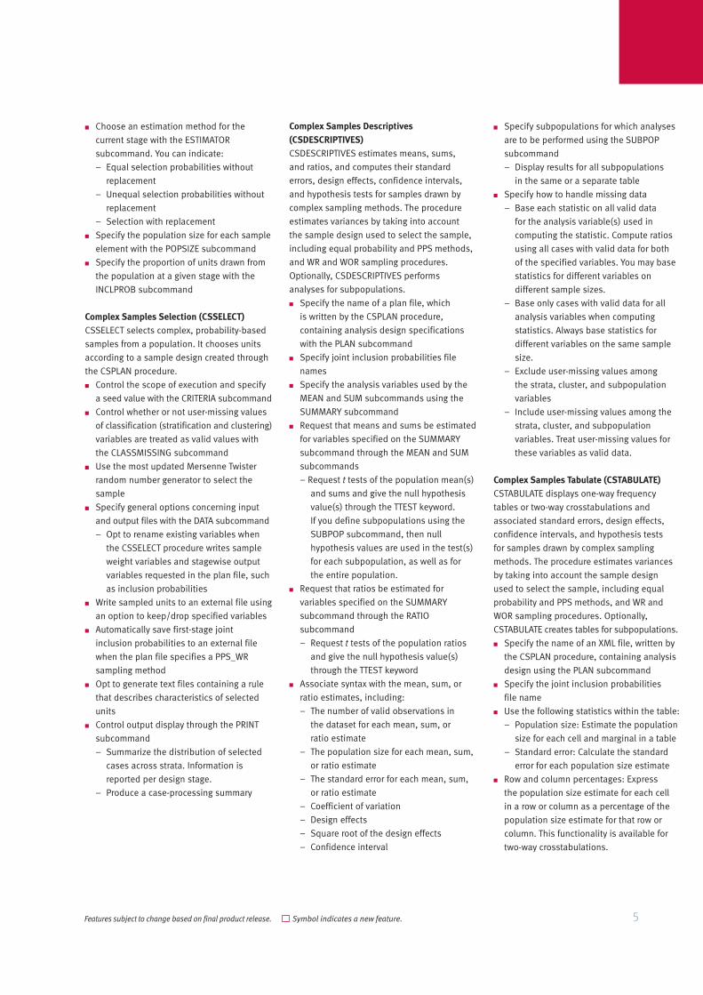
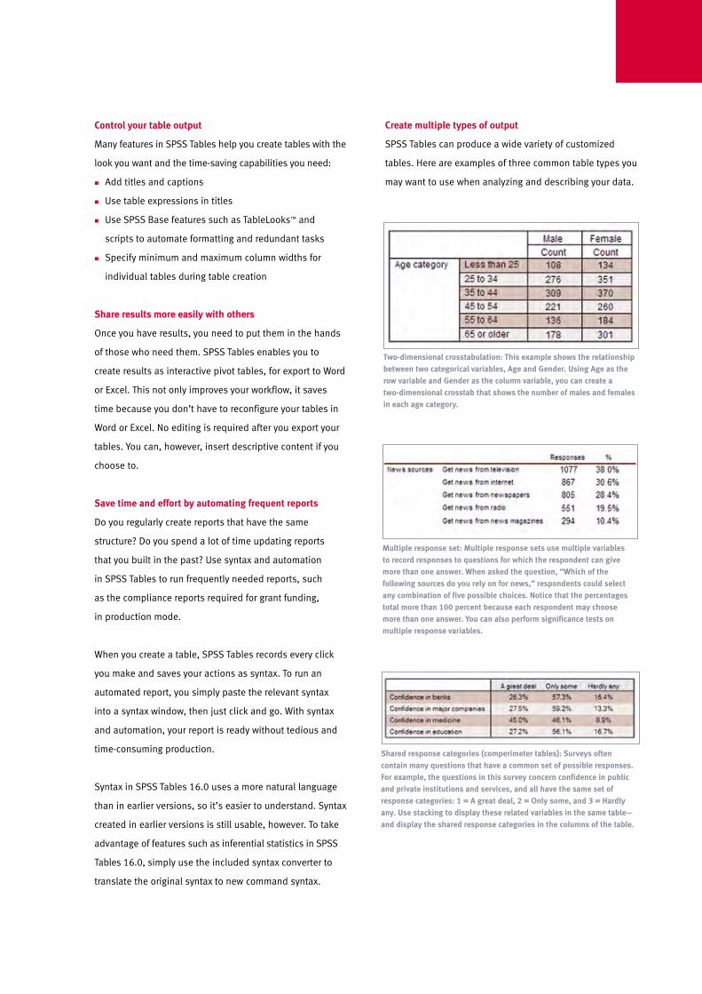
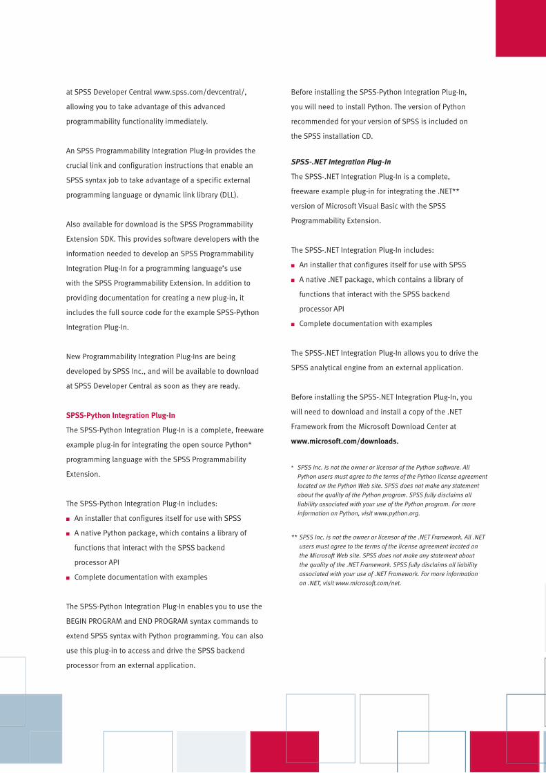
Neural networks are non-linear data mining tools that
consist of input and output layers plus one or more hidden
layers. In a neural network, the connections between
neurons have weights associated with them. These weights
are iteratively adjusted by the training algorithm
to minimize error and provide accurate predictions.
With the SPSS Neural Networks module, you can choose
either the Multilayer Perceptron (MLP) or Radial Basis
Function (RBF) procedure to explore your data in entirely
new ways.
New or enhanced statistical techniques
SPSS 16.0 offers enhanced statistical techniques in SPSS
Complex Samples™, SPSS Advanced Models™, Amos™, and
through the SPSS Programmability Extension™.
SPSS Complex Samples now includes the Cox Regression
technique for time-to-event data. If you have data based
on a complex sample design, you can use this technique
to accurately predict the time to a specific event—how long
a high-value customer remains active, for example, or how
long people fitting a certain profile will survive a certain
medical condition. SPSS Complex Samples Cox Regression
(CSCOXREG) enables you to more easily analyze differences
in subgroups as well as the effects of a set of predictors.
The procedure takes the sample design into account when
estimating variances and can handle data involving
multiple cases, such as multiple patient visits, encounters,
and observations.
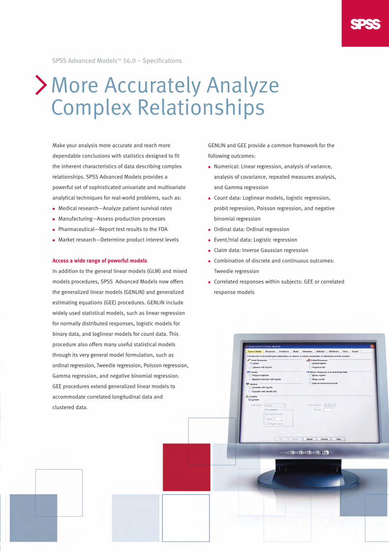
SPSS Advanced Models offers additional enhancements to
the generalized linear models (GENLIN) and generalized
estimating equations (GEE) procedures introduced
with SPSS 15.0. These procedures enable you to more
accurately predict ordinal outcomes, such as customer
satisfaction. Enhancements available in SPSS 16.0 enable
analysts to predict outcomes that are a combination
of discrete and continuous outcomes—such as claim
amounts—using a Tweedie distribution.
Amos, SPSS Inc.’s powerful but easy-to-use tool for
structural equation modeling (SEM), now offers latent class
analysis and mixture modeling. This statistical method is
particularly useful in market segmentation studies when
estimating the probability that an individual belongs to a
certain segment or cluster is important. This method also
provides a useful alternative to k-means cluster analysis.
2
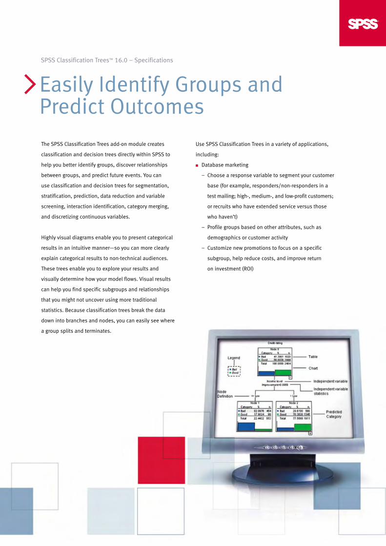
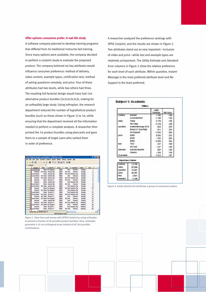
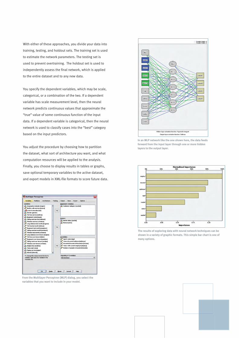
SPSS Neural Networks offers a choice of procedures to discover relationships in your data. This diagram shows a multilayer perceptron (MLP) procedure, with each node linked to other nodes in the input layer, the output layer, and the hidden layer between them.
In the SPSS Programmability Extension, described elsewhere,
the current integration plug-ins for Python® and the
Microsoft.NET version of Visual Basic® are joined by an
integration plug-in for R. This enables analysts to access
the wealth of statistical routines created in R and use
them within SPSS as part of SPSS syntax.
The SPSS Programmability Extension made possible the
introduction in SPSS 16.0 of Partial Least Squares (PLS)
regression as an alternative to Ordinary Least Squares
(OLS) regression. PLS is a predictive technique that can
handle many independent variables, even when they
display multicollinearity. Choose PLS instead of OLS if
you have a high number of variables relative to the
number of cases—a situation that frequently occurs in
survey research.
Enhanced data management and reporting capabilities
In addition to support for Unicode, as already mentioned,
SPSS 16.0 includes many enhancements to data
management that users have specifically requested. Now
you’ll have greater flexibility in how you work with, analyze,
and save your data. Using SPSS 16.0 capabilities, you can:
n Change the string length or the data type of an existing
variable, using syntax
n Define missing values and value labels for data strings
of any length
n Choose either to round off or add decimal places to
calculated dates when using the Date/Time Wizard
n Benefit from new capabilities in the Data Editor,
including the ability to find and replace information,
spell check value and variable labels, sort by variable
name, type, or format, and more
n Find and replace text in the Output Viewer—for example,
search for warnings to identify problems in your output
n Import/export data to and from Excel® 2007
n Suppress the number of active datasets in the
user interface
n Set a permanent default working directory
As for reporting, a new, more powerful visualization engine
replaces the Interactive Graph Properties (IGRAPH) feature,
making graph editing faster and easier. (Existing IGRAPH
syntax will continue to work.)
SPSS 16.0 introduces Python as the default front-end
scripting language. Python supersedes SAX Basic as the
scripting language for tasks such as automation of
repetitive tasks and customization of output. As with SAX
Basic, you can apply a “base” autoscript to all objects or to
individual objects. Existing SAX Basic scripts will continue
to work in SPSS 16.0
Improved programmability
The SPSS Programmability Extension enables you to
enhance the capabilities of SPSS by using external
programming languages such as Python. Applications
written in Python and Visual Basic can also call upon
the SPSS backend to conduct analysis or create
reports. Integration plug-ins are available at the SPSS
Developer Central Web site, as is the SPSS Programmability
Extension SDK that allows users to create their own
integration plug-ins.
SPSS continues to make the development of APIs easier for
users with additional improvements to the Programmability
Extension, and now allows the implementation of multiple
integration plug-ins and multiple versions of a single
integration plug-in.
An additional enhancement available through the SPSS
Programmability Extension is the new data step procedure
in the SPSS Python integration plug-in. This allows users
to create a completely new SPSS data file including the
simultaneous creation of defined variables and cases.
Visit SPSS Developer Central at www.spss.com/devcentral
to share code, tools, and programming ideas.
3
Greater performance and scalability
SPSS 16.0 features several multithreaded procedures,
which result in greater performance on machines
containing multiple processors and multi-core processors.
The following procedures are multithreaded: in SPSS Base,
Linear Regression, Correlation, Partial Correlation, and
Factor Analysis; and in SPSS Complex Samples, the SPSS
Complex Samples Select procedure.
SPSS 16.0 also provides additional integration with SPSS
Predictive Enterprise Services™. As organizations recognize
the need to create more effective processes for managing
and automating their analytic assets, providing an
efficient, cost-effective way to manage and update these
Enterprise Services provides these capabilities for
analytical assets created with SPSS—such as syntax,
scripts, and output—as well as for assets created with
other SPSS products such as the Clementine® data
mining workbench.
Enhancements to the SPSS Adapter for Predictive
Enterprise Services enable you to store and manage
a variety of assets, including Python script files,
and enjoy increased performance during retrieval and
refresh processes.
To learn more, please visit
www.spss.com/predictive_enterprise_services.
System requirements
SPSS Base 16.0 for Windows
n Operating System: Microsoft Windows XP (32-bit
versions) or Vista™ (32-bit or 64-bit versions)
n Hardware:
– Intel® or AMD x86 processor running at 1GHz or higher
– Memory: 256MB RAM or more; 512MB recommended
– Minimum free drive space: 450MB
– CD-ROM drive
– Super VGA (800x600) or higher-resolution monitor
– For connecting with an SPSS Server, a network adapter
running the TCP/IP network protocol
n Web browser: Internet Explorer 6
SPSS Base 16.0 for MAC OS X
n Operating system: Apple Mac OS X 10.4 (Tiger™)
n Hardware
– PowerPC or Intel processor
– Memory: 512MB RAM or more
– Minimum free drive space: 800MB
– CD-ROM drive
– Super VGA (800x600) or higher-resolution monitor
n Web browser: Safari™ 1.3.1, Firefox 1.5, or Netscape 7.2
n Java Standard Edition 5.0 (J2SE 5.0)
4
SPSS Base 16.0 for Linux
n Operatingsystem:anyLinuxOSthatmeetsthe
followingrequirements**:
– Kernel2.4.33.3orhigher
– glibc2.3.2orhigher
– XFree86-4.0orhigher
– libstdc++5
n Hardware:
– Processor:IntelorAMDx86processorrunningat
1GHzorhigher
– Memory:256MBRAMormore;512MBrecommended
– Minimumfreedrivespace:450MB
– CD-ROMdrive
– SuperVGA(800x600)orahigher-resolutionmonitor
n Webbrowser:Konqueror3.4.1,Firefox1.0.6,or
Netscape7.2
**Note:SPSS16.0wastestedonandissupportedonlyon
RedHatEnterpriseLinux4DesktopandDebian3.1
SPSS add-on modules
AllSPSS16.0add-onmodulesrequireSPSSBase16.0.
Noothersystemrequirementsarenecessary.
Amos 16.0
n Operating system: Windows XP or Windows Vista
n Hardware:
– Memory: 256MB RAM minimum
– 125MB or more available hard-drive space
– Web browser: Internet Explorer 6.0
SPSS Server 16.0
n Operating system: Windows Server 2003 (32-bit or 64-
bit); Sun™ Solaris™ (SPARC) 9 and later (64-bit only);
IBM® AIX® 5.3 and later; or Red Hat® Enterprise Linux®
ES4 and later; HP-UX IIi (64-bit Itanium)
n Hardware:
– Minimum CPU: Two CPUs recommended, running
at 1GHz or higher
– Memory: 256MB RAM per expected concurrent user
– Minimum free drive space: 300MB
– Required temporary disk space: Calculate by
multiplying 2.5 x number of users x expected size
of dataset in megabytes
SPSS Adapter for SPSS Predictive Enterprise Services
n Requires SPSS Base 16.0 and SPSS Predictive
Enterprise Services
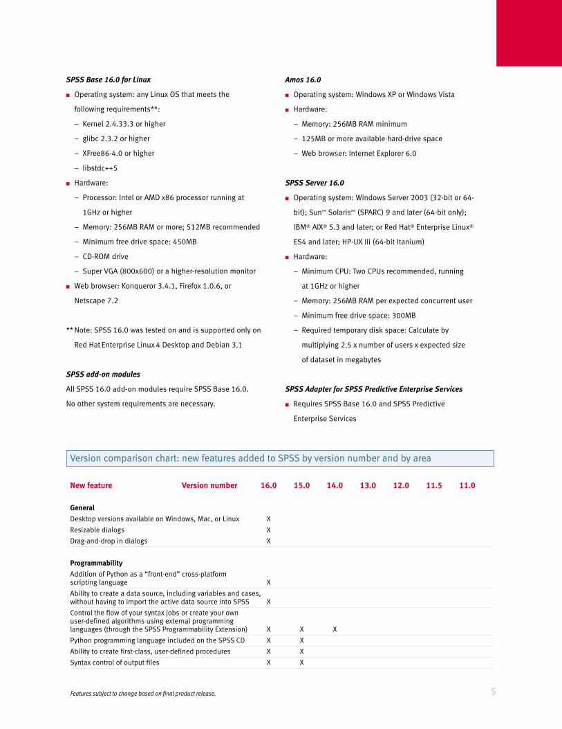
5
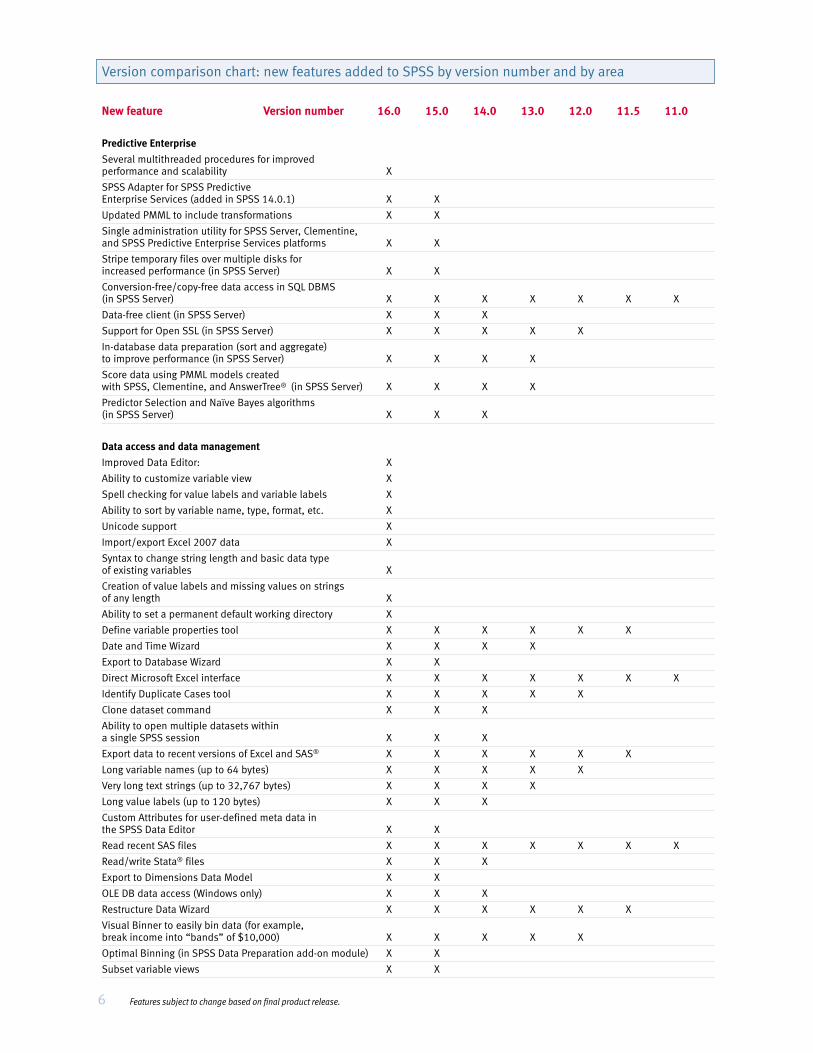
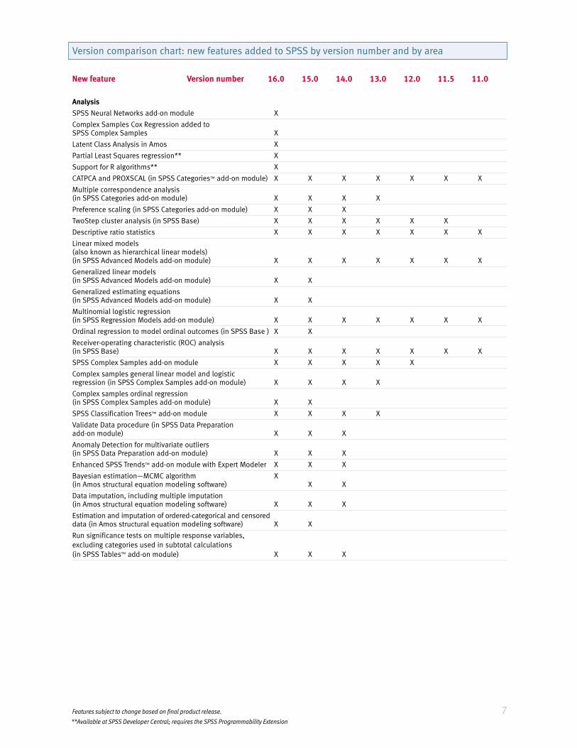
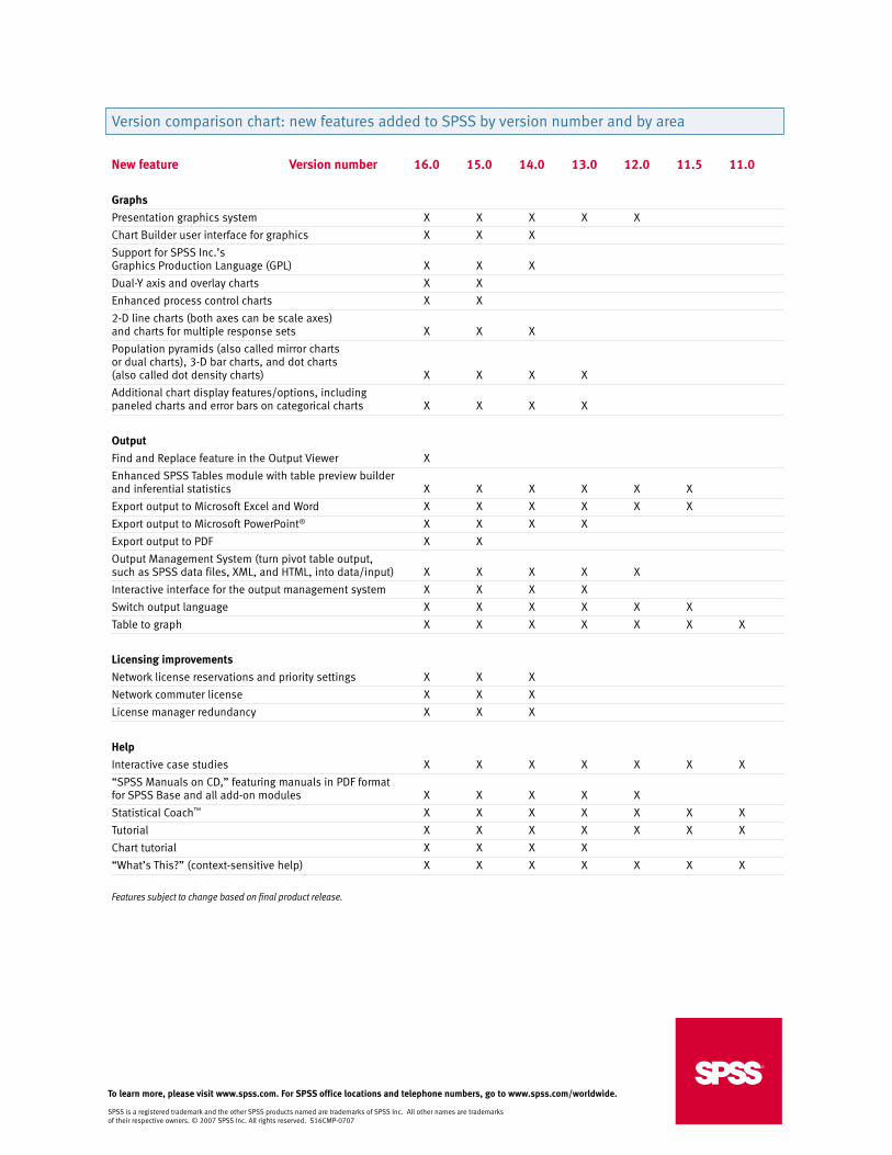
Version comparison chart: new features added to SPSS by version number and by area
New feature Version number 16.0 15.0 14.0 13.0 12.0 11.5 11.0
General
Desktop versions available on Windows, Mac, or Linux X
Resizable dialogs X
Drag-and-drop in dialogs X
Programmability
Addition of Python as a “front-end” cross-platform scripting language X
Ability to create a data source, including variables and cases, without having to import the active data source into SPSS X
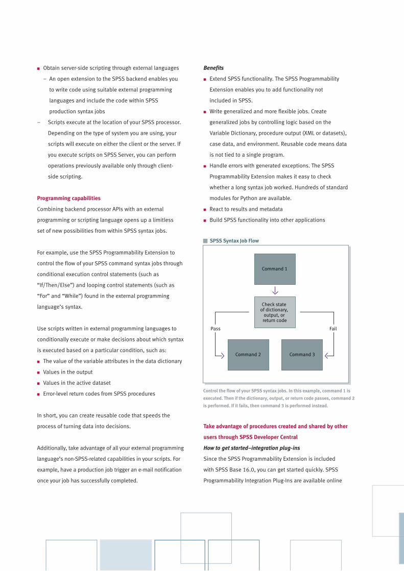
Control the flow of your syntax jobs or create your own user-defined algorithms using external programming languages (through the SPSS Programmability Extension) X X X
Python programming language included on the SPSS CD X X
Ability to create first-class, user-defined procedures X X
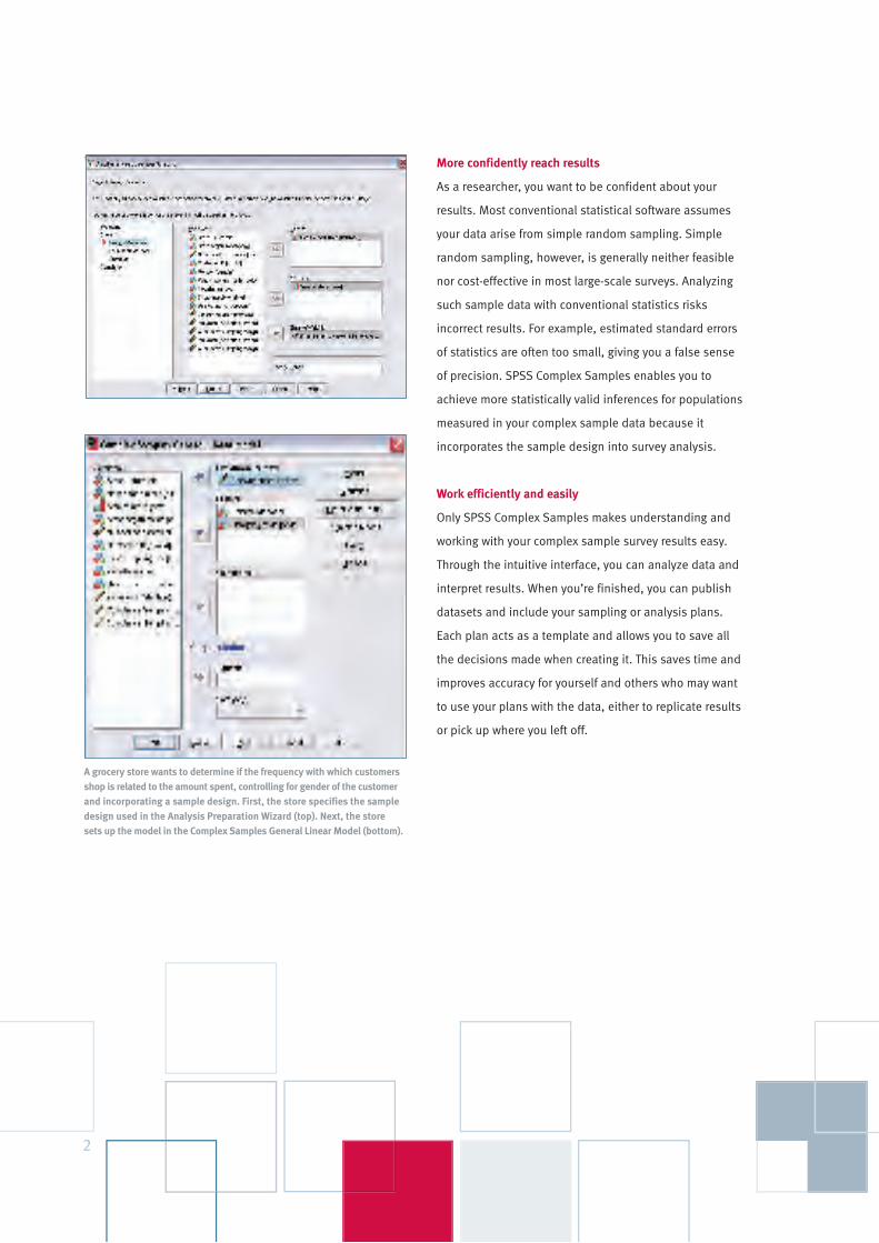
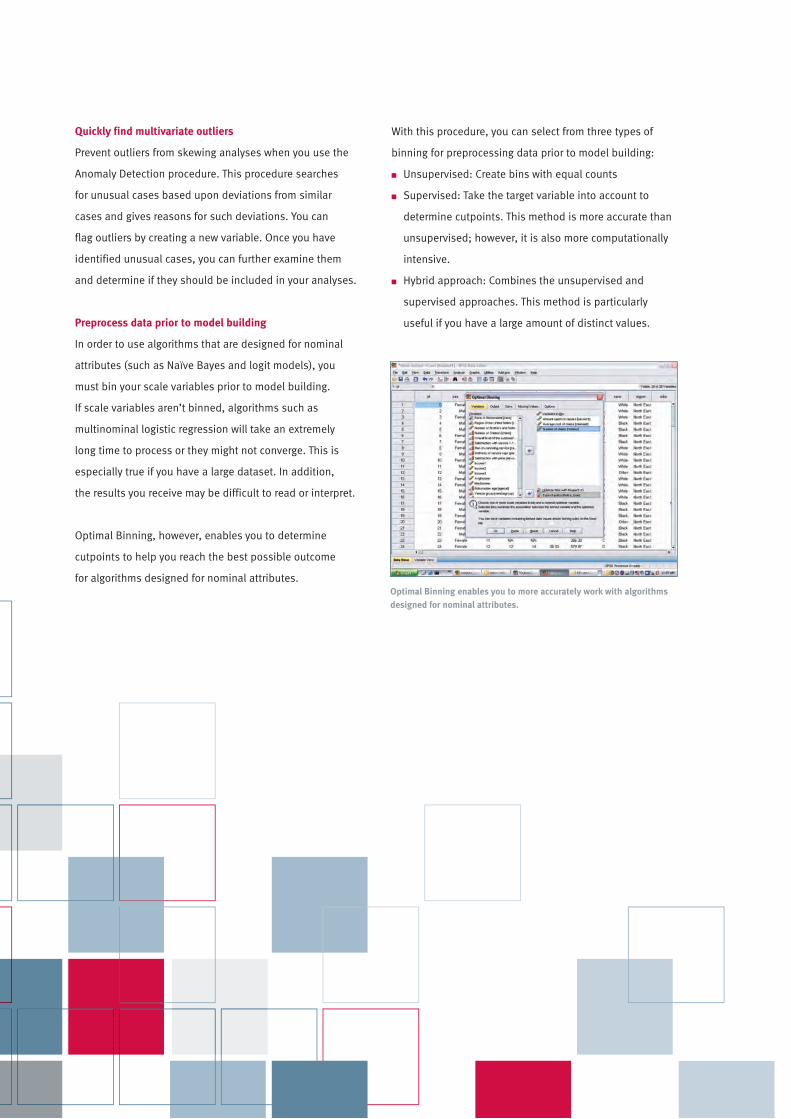
FeaturesGeneral operations■ Apply splitters through the Data Editor to
more quickly and easily understand wide
and long datasets
■ Select the customizable toolbar feature to:
– Assign procedures, scripts, or other
software products
– Select from standard toolbar icons or
create your own
■ Work with multidimensional pivot tables/
report cubes to:
– Rearrange columns, rows, and layers by
dragging icons for easier ad hoc analyses
– Toggle between layers by clicking on an
icon for easier comparison between
subgroups
– Enable online statistical help for
choosing statistical procedures or chart
types and interpreting results; realistic
application examples are included
■ Change text attributes such as fonts, colors,
bolding, italics, and others
■ Change table attributes such as number
formats, line styles, line width, column
alignments, background/foreground
shading, enable or disable lines, and more
■ Selectively display or hide rows, columns,
or labels to highlight important findings
■ Enable task-oriented help with step-by-step
instructions:
– View case studies that show you how to
use selected statistics and interpret results
– Select the Statistics Coach™, which
helps you choose the best statistical
procedure or graph
– Work through tutorials
– Select “Show Me” buttons, which link to
the tutorial for more in-depth help when
you need it
– Use “What’s This?” help, which provides
pop-up definitions of statistical terms
and rules of thumb
■ Use formatting capabilities for output to:
– Transform a table into a graph for more
visually compelling communication
– Show correlation coefficients together
with their significance level (as well as n)
in correlations using the default output
display
– Control whether, upon activation, a table
is opened in place or in its own window
– Stamp date and time into the journal file
for easy reference
– Right-click on an SPSS syntax file icon to
run a command file without needing to
go through production mode
– Use drop-down lists for easier access to
different layers
– Set permanent page settings
– Set a column width for all pivot tables
and define text wrapping
– Choose whether to use scientific
notation to display small numbers
– Control number of digits of precision in
presentations
– Interact with reports and use models
and code created by others in your
organization with the optional addition
of SPSS Predictive Enterprise Services.
– Add footnotes and annotations
– Reorder categories within a table to
display results most effectively
– Group or ungroup multiple categories in
rows or columns under a single heading
that spans the rows or columns
– Use one of 16 pre-formatted TableLooks™
for quick and consistent formatting of
results
– Create and save customized formats as
TableLooks for your own personalized style
– Display values or labels
– Rotate table labels
■ Work with the Viewer to organize, view, and
move through results
– Keep a record of your work using the
“append” default in journal files
– Use outline representation to quickly
determine output location
– Select an icon in the outline and see
corresponding results displayed in the
content pane
– Reorder charts, tables, and other objects
by dragging icons in the outline
– Selectively collapse or expand the
outline to view or print selected results
– Contain tables, charts, and objects in a
single content pane for easy review and
access
– Right-justify, left-justify, or center output
– Search and replace information in the
Viewer of the contents pane, the outline
pane, or both
■ Create and save analysis specifications for
repetitive tasks or unattended processing
■ Use the enhanced production mode facility
with dialog interface and macros for easier
periodic reporting
■ Have full control over table splitting with
improved pagination and printing
■ Select the print preview option
■ Enter your own commands, if you wish,
via a command line input window
■ Refer to explanations of statistical terms
through the on-screen statistical glossary
■ Work with data more easily, thanks to:
– Resizable dialog boxes
– Drag-and-drop in dialogs
■ Export output to Microsoft Word
– Convert pivot tables to Word tables
with all formatting saved
– Convert graphics into static pictures
■ Export output to PowerPoint®
(Windows only)
– Convert pivot tables to tables in
PowerPoint with all formatting saved
– Convert graphics into static pictures
Features subject to change based on final product release. Symbol indicates a new feature. 3
■ Export output to Excel®
– Put tables on the same sheet or on
separate sheets within one Excel
workbook file
– Export only the current view or all layers
of an SPSS pivot table
– Place each pivot table layer on the
same sheet or on separate sheets
within one Excel workbook
■ Export SPSS output to PDF
– Choose to optimize the PDF for Web
viewing
– Control whether PDF-generated
bookmarks correspond to Navigator
Outline entries in the Output Viewer.
Bookmarks facilitate navigation of
large documents.
– Control whether fonts are embedded in
the document. Embedded fonts ensure
that the reader of your document sees
the text in its original font, preventing
font substitution.
■ Easily open/save and create new output
files through syntax
■ Receive wheel mouse support for Output
Viewer scroll
■ Switch output languages (for example,
switch between Japanese and English)
■ Use the scripting facility to:
– Create, edit, and save scripts
– Build customized form interfaces
– Assign scripts to toolbar icons or menus
– Automatically execute scripts whenever
certain events occur
– Support Python 2.5 to make scripting
easier and more reliable
■ Use automation to:
– Integrate SPSS with other desktop
applications
– Build custom applications using Visual
Basic®, PowerBuilder®, and C++
– Integrate SPSS into larger custom
applications (such as Word or Excel)
■ Use the HOST command to take advantage
of the operating system functionality in
SPSS. This command enables applications
to “escape” to the operating system and
execute other programs in sync with the
SPSS session.
■ Prevent syntax jobs from breaking when you
create a common or main project directory
that enables you to include transformations
for multiple projects
– Better manage multiple projects, syntax
files, and datasets
■ Specify interactive syntax rules using the
INSERT command
Graphic capabilities ■ Categorical charts
– 3-D Bar: Simple, cluster, and stacked
– Bar: Simple, cluster, stacked, drop-
shadow, and 3-D
– Line: Simple, multiple, and drop-line
– Area: Simple and stacked
– Pie: Simple, exploding, and 3-D effect
– High-low: High-low-close, difference
area, and range bar
– Boxplot: Simple and clustered
– Error bar: Simple and clustered
– Error bars: Add error bars to bar, line,
and area charts; confidence level;
standard deviation; and standard error
– Dual-Y axis and overlay
■ Scatterplots
– Simple, grouped, scatterplot matrix,
and 3-D
– Fit lines: Linear, quadratic or cubic
regression, and Lowess smoother;
confidence interval control for total or
subgroups; and display spikes to line
– Bin points by color or marker size to
prevent overlap
■ Density charts
– Population pyramids: Mirrored axis to
compare distributions; with or without
normal curve
– Dot charts: Stacked dots show
distribution; symmetric, stacked,
and linear
– Histograms: With or without normal
curve; custom binning options
■ Quality control charts
– Pareto
– X-Bar
– Range
– Sigma
– Individuals
– Moving range
– Control chart enhancements include
automatic flagging of points that violate
Shewhart rules, the ability to turn off
rules, and the ability to suppress charts
■ Diagnostic and exploratory charts
– Caseplots and time-series plots
– Probability plots
– Autocorrelation and partial
autocorrelation function plots
– Cross-correlation function plots
– Receiver-Operating Characteristics (ROC) ■ Multiple use charts
– 2-D line charts (both axes can be
scale axes)
– Charts for multiple response sets ■ Custom charts
– Graphics Production Language (GPL), a
custom chart creation language, enables
advanced users to attain a broader range
of chart and option possibilities than the
interface supports
■ Editing options
– Automatically reorder categories in
differing order (descending or ascending)
or by different sort methods (value,
label, or summary statistic)
– Create data value labels
– Drag to any position on your chart,
add connecting lines, and match font
color to subgroup
– Select and edit specific elements directly
within a chart: Colors, text, and styles
– Choose from a wide range of line styles
and weights
– Display gridlines, reference lines, leg
ends, titles, footnotes, and annotations
– Include an Y=X reference line
■ Layout options
– Paneled charts: Create a table of
subcharts, one panel per level or
condition, showing multiple rows
and columns
– 3-D effects: Rotate, modify depth, and
display backplanes
■ Chart templates
– Save selected characteristics of a chart
and apply them to others automatically.
You can apply the following attributes
at creation or editing time: Layout, titles,
footnotes and annotations, chart
element styles, data element styles,
axis scale range, axis scale settings,
fit and reference lines, and scatterplot
point binning
– Tree-view layout and finer control
of template bundles
■ Graph export: BMP, EMF, EPS, JPG, PCT,
PNG, TIF, and WMF
Features subject to change based on final product release. Symbol indicates a new feature.4
AnalysisDescriptive statistics
Reports
■ OLAP cubes enable you to:
– Quickly estimate changes in the mean or
sum between any two related variables
using percent change. For example, easily
see how sales increase from quarter
to quarter.
– Create case summaries
– Create report summaries
– Generate presentation-quality reports
using numerous formatting options
– Generate case listing and case summary
reports with statistics on break groups
Frequencies
■ Frequency tables: Frequency counts, percent,
valid percent, and cumulative percent
■ Option to order your output by analysis or
by table
■ More compact output tables by eliminating
extra lines of text where they’re not needed
■ Central tendency: Mean, median, mode,
and sum
■ Dispersion: Maximum, minimum, range,
standard deviation, standard error, and
variance
■ Distribution: Kurtosis, kurtosis standard
error, skewness, and skewness standard
error
■ Percentile values: Percentiles (based on
actual or grouped data), quartiles, and
equal groups
■ Format display: Condensed or standard,
sorted by frequency or values, or index
of tables
■ Charts: Bar, histogram, or pie chart
Descriptives
■ Central tendency: Mean and sum
■ Dispersion: Maximum, minimum, range,
standard deviation, standard error, and
variance
■ Distribution: Kurtosis and skewness
■ Z scores: Compute and save as new
variables
■ Display order: Ascending or descending
order on means and variable name
Explore
■ Confidence intervals for mean
■ Descriptives: Interquartile range, kurtosis,
kurtosis standard error, median, mean,
maximum, minimum, range, skewness,
skewness standard error, standard
deviation, standard error, variance, five
percent trimmed mean, and percentages
■ M-estimators: Andrew’s wave estimator,
Hampel’s M-estimator, Huber’s M-estimator,
and Tukey’s biweight estimator
■ Extreme values and outliers identified
■ Grouped frequency tables: Bin center,
frequency, percent, valid, and cumulative
percent
■ Plots: Construct plots with uniform scale or
dependence on data values
– Boxplots: Dependent variables and factor
levels together
– Descriptive: Histograms and stem-and-
leaf plots
– Normality: Normal probability plots and
detrended probability plots with
Kolmogorov-Smirnov and Shapiro-Wilk
statistics
– Spread versus level plots using Levene’s
test: Power estimation, transformed, or
untransformed
– Shapiro-Wilk test of normality in
EXAMINE allows for 5,000 cases when
weights are not specified
Crosstabs
■ Three-way relationships in categorical
data with Cochran’s and Mantel-Haenszel
statistics allow you to go beyond the limits
of a two-way crosstab
■ Counts: Observed and expected frequencies
■ Percentages: Column, row, and total
■ Long string variables
■ Residuals: Raw, standardized, and adjusted
standardized
■ Marginals: Observed frequencies and total
percentages
■ Tests of independence: Pearson and Yates
corrected Chi-square, likelihood ratio Chi-
square, and Fisher’s exact test
■ Test of linear association: Mantel-Haenszel
Chi-square
■ Measure of linear association: Pearson r
■ Nominal data measures: Contingency
coefficient, Cramer’s V, Phi, Goodman
and Kruskal’s Lambda (asymmetric and
symmetric), Tau (column or row dependent),
and uncertainty coefficient (asymmetric and
symmetric)
■ Ordinal data measures: Goodman and
Kruskal’s Gamma, Kendall’s Tau-b and
Tau-c, Somers’ D (asymmetric and
symmetric), and Spearman’s Rho
■ Nominal by interval measure: Eta
■ Measure of agreement: Cohen’s Kappa
■ Relative risk estimates for case control and
cohort studies
■ Display tables in ascending or descending
order
■ Frequency counts written to file
■ McNemar’s test
■ Option to use integer or non-integer weights
Descriptive ratio statistics
■ Help for understanding your data using:
– Coefficient of dispersion
– Coefficient of variation
– Price-related differential (PRD)
– Average absolute deviance
Features subject to change based on final product release. Symbol indicates a new feature. 5
Compare means
Means
■ Create better models with harmonic and
geometric means
■ Cells: Count, mean, standard deviation,
sum, and variance
■ All-ways totals
■ Measure of analysis with Eta and Eta2
■ Test of linearity with R and R2
■ Results displayed in report, crosstabular,
or tree format
■ Statistics computed for total sample
t test
■ One sample t test to compare sample mean
to a reference mean of your choice
■ Independent sample statistics: Compare
sample means of two groups for both
pooled and separate-variance estimates
with Levene’s test for equal variances
■ Paired sample statistics: Correlation
between pairs, difference between means,
and two-tailed probability for test of no
difference and for test of zero correlation
between pairs
■ Statistics: Confidence intervals, counts,
degrees of freedom, mean, two-tailed
probability, standard deviation, standard
errors, and t statistic
One-way ANOVA
■ Contrasts: Linear, quadratic, cubic,
higher-order, and user-defined
■ Range tests: Duncan, LSD, Bonferroni,
Student-Newman-Keuls, Scheffé, Tukey’s
alternate test, and Tukey’s HSD
■ Post hoc tests: Student-Newman-Keuls,
Tukey’s honestly significant difference,
Tukey’s b, Duncan’s multiple comparison
procedure based on the Studentized range
test, Scheffé’s multiple comparison t test,
Dunnett’s two-tailed t test, Dunnett’s
one-tailed t test, Bonferroni t test, least
significant difference t test, Sidak t test,
Hochberg’s GT2, Gabriel’s pairwise
comparisons test based on the Studentized
maximum modulus test, Ryan-Einot-
Gabriel-Welsch’s multiple stepdown
procedure based on an F test, Ryan-Einot-
Gabriel-Welsch’s multiple stepdown
procedure based on the Studentized range
test, Tamhane’s T2, Tamhane’s T3, Games
and Howell’s pairwise comparisons test
based on the Studentized range test,
Dunnett’s C, and Waller-Duncan t test
■ ANOVA statistics: Between- and within-
groups sums of squares, degrees of
freedom, mean squares, F ratio, and
probability of F
■ Fixed-effects measures: Standard deviation,
standard error, and 95 percent confidence
intervals
■ Random effects measures: Estimate of
variance components, standard error,
and 95 percent confidence intervals
■ Group descriptive statistics: Maximum,
mean, minimum, number of cases,
standard deviation, standard error, and
95 percent confidence interval
■ Homogeneity of variance test: Levene’s test
■ Read and write matrix materials
■ Equality of means: Reach accurate results
when variances and sample sizes vary
across different groups
– Brown-Forsythe test
– Welch test
ANOVA models—simple factorial
■ Create custom models without limits on
maximum order of interaction
■ Work faster because you don’t have to
specify ranges of factor levels
■ Choose the right model using four types of
sum of squares
■ Increase certainty with better data handling
in empty cells
■ Perform lack-of-fit tests to select your best
model
■ Choose from one of two designs: Balanced
or unbalanced
■ Use analysis of covariance with up to 10
covariate methods: Classic experimental,
hierarchical, and regression
■ Enter covariates control: Before, with, or
after main effects
■ Set interaction to: None, 2-, 3-, 4-, or 5-way
■ Select from the following statistics:
ANOVA, means and counts table, multiple
classification analysis, unstandardized
regression coefficients, and n-way cell means
■ Choose up to 10 independent variables
■ Reach predicted values and deviations from
the mean in MCA table
Correlate*
Bivariate
■ Pearson r, Kendall’s Tau-b, and Spearman
■ One- and two-tailed probabilities
■ Means, number of non-missing cases,
and standard deviations
■ Cross-product deviations and covariances
■ Coefficients displayed in matrix or serial
format
Partial*
■ One- and two-tailed probabilities
■ Mean, number of non-missing cases,
and standard deviation
■ Zero-order correlations
■ Up to 100 control variables
■ Up to five order values
■ Correlations displayed in matrix or
serial string format, lower triangular,
or rectangular correlation matrix
Distances
■ Compute proximities between cases
or variables
■ Dissimilarity measures
– Interval measure: Euclidean and squared
Euclidean distance, Chebychev distance
metric, city-block or Manhattan distance,
distance in an absolute Minkowski power
metric, and customized
– Counts measures: Chi-square and
Phi-square
– Binary measures: Euclidean and squared
Euclidean distance; size, pattern, and
shape difference; variance dissimilarity
measure; and Lance and Williams
nonmetric
■ Similarity measures
– Interval measures: Pearson correlation
and cosine
– Binary measures: Russell and Rao;
simple matching; Jaccard; dice (or
Czekanowski or Sorenson); Rodgers and
Tanimoto; Sokal and Sneath 1 through 5;
Kulczynski 1 and 2; Hamann; Goodman
and Krusal Lambda; Anderberg’s D;
Yule’s coefficient of colligation; Yule’s Q;
Ochiai; dispersion similarity measure;
and fourfold point correlation
■ Standardize data values: Z scores, range
of -1 to 1, range of 0 to 1, maximum
magnitude of 1, mean of 1, and standard
deviation of 1
Features subject to change based on final product release. Symbol indicates a new feature.6
■ Transform measures: Absolute values,
dissimilarities into similarities, similarities
into dissimilarities, and rescale proximity
values to a range of 0 to 1
■ Identification variable specification
■ Printed matrix of proximities between items
■ Improved scalability for proximities
between variable matrices
Regression—linear regression*
■ Methods: Backward elimination, forced
entry, forced removal, forward entry,
forward stepwise selection, and R2 change/
test of significance
■ Equation statistics: Akaike information
criterion (AIC), Ameniya’s prediction
criterion, ANOVA tables (F, mean square,
probability of F, regression, and residual
sum of squares), change in R2, F at step,
Mallow’s Cp, multiple R, probability of F,
R2, adjusted R2, Schwarz Bayesian criterion
(SBC), standard error of estimate, sweep
matrix, and variance-covariance matrix
■ Descriptive statistics: Correlation matrix,
covariance matrix, cross-product deviations
from the mean, means, number of cases
used to compute correlation coefficients,
one-tailed probabilities of correlation
coefficients, standard deviations, and
variances
■ Independent variable statistics: Regression
coefficients, including B, standard errors
of coefficients, standardized regression
coefficients, approximate standard error
of standardized regression coefficients,
and t; tolerances; zero-order; part and
partial correlations; and 95 percent
confidence interval for unstandardized
regression coefficient
■ Variables not in equation: Beta or minimum
tolerance
■ Durbin-Watson
■ Collinearity diagnostics: Condition indexes,
eigenvalues, variance inflation factors,
variance proportions, and tolerances
■ Plots: Casewise, histogram, normal
probability, de-trended normal, partial,
outlier, and scatterplots
■ Create and save variables:
– Prediction intervals: Mean and individual
– Predicted values: Unstandardized,
standardized, adjusted, and standard
error of mean
– Distances: Cook’s distances, Mahalanobis’
distance, and leverage values
– Residuals: Unstandardized, standardized,
Studentized, deleted, and Studentized
deleted
– Influence statistics: dfbetas, standardized
dfbetas, dffits, standardized dffits, and
covariance ratios
■ Option controls: F-to-enter, F-to-remove,
probability of F-to-enter, probability of F-to-
remove, suppress the constant, regression
weights for weighted least-squares model,
confidence intervals, maximum number of
steps, replace missing values with variable
mean, and tolerance
■ Regression coefficients displayed in user-
defined order
■ System files can contain parameter estimates
and their covariance and correlation matrices
through the OUTFILE command
■ Solutions can be applied to new cases or
used in further analysis
■ Decision making can be further improved
throughout your organization when you
export your models via XML
Ordinal regression—PLUM*
■ Predict ordinal outcomes
– Seven options to control the iterative
algorithm used for estimation, to specify
numerical tolerance for checking
singularity, and to customize output
– Five link functions to specify the model:
Cauchit, complementary log-log, logit,
negative log-log, and probit
– Location subcommand to specify the
location model: Intercept, main effects,
interactions, nested effects, multiple-
level nested effects, nesting within an
interaction, interactions among nested
effects, and covariates
– Print: Cell information, asymptotic
correlation matrix of parameter
estimates, goodness-of-fit statistics,
iteration history, kernel of the log-
likelihood function, test of parallel lines
assumption, parameter statistics, and
model summary
– Save casewise post-estimation statistics
into the active file: Expected probabilities
of classifying factor/covariate patterns
into response categories and response
categories with the maximum expected
probability for factor/covariate patterns
– Customize your hypotheses tests by
directly specifying null hypotheses as
linear combinations of parameters using
the TEST subcommand (syntax only)
Curve estimation
■ Eleven types of curves are available for
specification
■ Regression summary displays: Curve type,
R2 coefficient, degrees of freedom, overall
F test and significance level, and regression
coefficients
■ Trend-regression models available: Linear,
logarithmic, inverse, quadratic, cubic,
compound, power, S, growth, exponential,
and logistic
Nonparametric tests
■ Chi-square: Specify expected range (from
data or user-specified) and frequencies
(all categories equal or user-specified)
■ Binomial: Define dichotomy (from data
or cutpoint) and specify test proportion
■ Runs: Specify cutpoints (median, mode,
mean, or specified)
■ One sample: Kolmogorov-Smirnov, uniform,
normal, and Poisson
■ Two independent samples: Mann-Whitney
U, Kolmogorov-Smirnov Z, Moses extreme,
and Wald-Wolfowitz runs
■ k-independent samples: Kruskal-Wallis H
and median
■ 2-related samples: Wilcoxon, sign, and
McNemar
■ k-related samples: Friedman, Kendall’s W,
and Cochran’s Q
■ Descriptives: Maximum, mean, minimum,
number of cases, and standard deviation
Multiple response
■ Crosstabulation tables: Cell counts, cell
percentages based on cases or responses,
column and row, and two-way table
percentages
■ Frequency tables: Counts, percentage of
cases, or responses
■ Both multiple-dichotomy and multiple-
response groups can be handled
Data reduction
Factor*
■ Number of cases and variable labels for
analysis can be displayed
■ Input from correlation matrix, factor,
loading matrix, covariance matrix, or
raw data case file
■ Output of correlation matrix or factor matrix
Features subject to change based on final product release. Symbol indicates a new feature. * Multithreaded algorithm, resulting in improved performance and scalability on multiprocessor or multicore machines. 7
■ Seven extraction methods available for use
when analysis is performed on correlation
matrices or raw data files: Principal
component, principal axis, Alpha factoring,
image factoring, maximum likelihood,
unweighted least squares, and generalized
least squares
■ Rotation methods: Varimax, equamax,
quartimax, promax, and oblimin
■ Display: Initial and final communalities,
eigenvalues, percent variance, unrotated
factor loadings, rotated factor pattern
matrix, factor transformation matrix, factor
structure, and correlation matrix (oblique
rotations only)
■ Covariance matrices can be analyzed
using three extraction methods: Principal
component, principal axis, and image
■ Factor scores: Regression, Bartlett, and
Anderson-Rubin
■ Factor scores saved as active variables
■ Statistics available: Univariate correlation
matrix, determinant and inverse of
correlation matrix, anti-image correlation
and covariance matrices, Kaiser-Meyer-
Olkin measure of sampling adequacy,
Bartlett’s test of sphericity, factor pattern
matrix, revised communalities, eigenvalues
and percent variance by eigenvalue,
reproduced and residual correlations, and
factor score coefficient matrix
■ Plots: Scree plot and plot of variables in
factor space
■ Matrix input and output
■ Post-rotational calculated through sum-
of-squares loadings
■ Solutions applied to new cases or to
use in further analysis with the SELECT
subcommand
■ Factor score coefficient matrix exported
to score new data (syntax only)
Classify
TwoStep cluster analysis
■ Group observations into clusters based on
a nearness criterion. This procedure uses
a hierarchical agglomerative clustering
procedure in which individual cases are
successively combined to form clusters
whose centers are far apart. This algorithm
is designed to cluster large numbers of
cases. It passes the data once to find
cluster centers and again to assign cluster
memberships. Cluster observations by
building a data structure called the CF Tree,
which contains the cluster centers. The CF
Tree is grown during the first stage of
clustering and values are added to its
leaves if they are close to the cluster center
of a particular leaf.
– Categorical-level and continuous-level
data can be used
– Distance measures: Euclidean distance
and the likelihood distance
– Criteria command tunes the algorithm
so that:
■ The initial threshold can be specified
to grow a CF Tree
■ The maximum number of child nodes
a leaf node may have can be set
■ The maximum number of levels a CF
Tree may have can be set
– HANDLENOISE subcommand enables
you to treat outliers in a special manner
during clustering. The default value of
noise percent is zero, equivalent to no
noise handling. The value can range
between zero and 100.
– INFILE subcommand allows the algorithm
to update a cluster model in which a CF
Tree is saved as an XML file using the
OUTFILE subcommand
– MEMALLOCATE subcommand specifies
the maximum amount of memory in
megabytes (MB) that the cluster algorithm
should use
– Missing data: Exclude both user-missing
and system-missing values, or let user-
missing values be treated as valid
– Option to standardize continuous-level
variables or leave them at the original
scale
– Ability to specify the number of clusters,
specify the maximum number of clusters,
or let the number of clusters be chosen
automatically
■ Algorithms available for determining
the number of clusters: BIC or AIC
– Output written to a specified filename
as XML
– Final model output saved, or use an
option that updates the model later
with more data
– Plots:
■ Bar chart of frequencies for each
cluster
■ Pie chart showing observation
percentages and counts within each
cluster
■ Importance of each variable within
each cluster: The output is sorted by
the importance rank of each variable
– Plot options:
■ Comparisons (one plot per cluster or
one plot per variable)
■ Measure of variable importance
(parametric or non-parametric)
■ Ability to specify Alpha level when
considering importance
– Print options:
■ AIC or BIC for different numbers
of clusters
■ Two tables describing the variables in
each cluster. In one table, means and
standard deviations are reported for
continuous variables. The other table
reports frequencies of categorical
variables. All values are separated
by cluster.
■ List of clusters and number of
observations in each cluster
– Cluster number saved for each case
to the working data file
Cluster
■ Use one of six linkage methods to
determine clusters: Single linkage (nearest
neighbor), average linkage between groups,
centroid (average linkage within groups),
complete linkage (farthest neighbor),
median, and Ward
■ Provide the same set of similarity and
dissimilarity measures as in proximity
■ Save cluster memberships as new variables
■ Save distance matrices for use in other
procedures
■ Display: Agglomeration schedules, cluster
membership, and distance matrices
■ Use proximities between variable matrices
for improved scalability
■ Choose from the following plots: Horizontal
and vertical icicle plots and dendrogram
plots of cluster solutions
■ Specify case identifiers for tables and plots
■ Have the ability to accept matrix input and
produce matrix output
Quick cluster
■ Squared Euclidean distance
■ Centers selected by widely spaced cases,
first K cases, or direct specification
■ Cluster membership saved as a variable
■ Two methods provided for updating cluster
centers
■ K-means clustering algorithms
8Features subject to change based on final product release. Symbol indicates a new feature. * Multithreaded algorithm, resulting in improved performance and scalability on multiprocessor or multicore machines.
Discriminant
■ Variable selection methods: Direct entry,
Wilks’ Lambda minimization, Mahalanobis’
distance, smallest F ratio, minimization of
sum of unexplained variation for all pairs,
and largest increase in Rao’s V
■ Statistics:
– Summary: Eigenvalues, percent and
cumulative percent of variance, canonical
correlations, Wilks’ Lambda, and Chi-
square tests
– At each step: Wilks’ Lambda, equivalent F,
degrees of freedom, and significance of
F for each step; F-to-remove; tolerance;
minimum tolerance; F-to-enter; and value
of statistic for each variable not in equation
– Final: Standardized canonical discriminant
function coefficients, structure matrix of
discriminant functions, and functions
evaluated within group means
– Optional: Means, standard deviations,
univariate F ratios, pooled within-groups
covariance and correlation matrices,
matrix of pairwise F ratios, Box’s M test,
group and total covariance matrices,
unstandardized canonical discriminant
functions, classification results table,
and classification function coefficients
■ Rotation of coefficient (pattern) and
structure matrices
■ Output displayed step by step and/or in
summary form
■ In classification stage: Prior probabilities,
equal, proportion of cases, or user-specified
■ All groups, cases, territorial maps, and
separate groups plotted
■ Casewise results saved to system file for
further analysis
■ Matrix files read/written, including
additional statistics: Counts, means,
standard deviations, and Pearson
correlation coefficients
■ Solutions applied to new cases or for use
in further analysis
■ Jacknife estimates provided for
misclassified error rate
■ Decision making further improved by
exporting your models throughout your
organization via XML
Scaling
■ Reduce your data and improve
measurement with reliability
■ Find the hidden structure in your similarity
data using ALSCAL multidimensional scaling
Matrix operations
■ Write your own statistical routines in the
compact language of matrix algebra
Data management■ Prepare continuous-level data for analysis
with the Visual Binner
– Specify cutpoints in an intelligent
manner using a histogram created
through a data pass
– Automatically create value labels based
on your cutpoints
– Copy bins to other variables
■ Create your own custom programs with the
Output Management System (OMS). Turn
output from SPSS procedures into data
(SPSS data files, XML, or HTML) and create
your programs for bootstrapping, jacknifing
and leaving-one-out methods, and Monte
Carlo simulations
– Create custom programs in SPSS, even
if you have little or no experience with
SPSS syntax, using the Output
Management System Control Panel
■ Easily clean your data when you identify
duplicate records through the user interface
with the Identify Duplicate Cases tool
■ Make sense and keep track of your data
files by adding notes to them with the Data
File Comments command
■ Prevent the accidental destruction of data
by making the dataset read-only
■ Easily set up all of your value labels to
prepare your data for analysis using the
Define Variable Properties tool
– Set up data dictionary information,
including value labels and variable types
– Intelligently add labels because a data
pass made first enables SPSS to present
a list of values and counts of those values
– Save time by being able to enter data
and value labels directly onto the grid
rather than having to use nested dialogs
■ Save work by easily copying dictionary
information from one variable to another
and from one dataset to another using the
Copy Data Properties tool
– Copy dictionary information (such as
variable and value labels) between
variables and datasets using the
template facility
– Receive a ready means of cloning
dictionaries
■ Analyze more data, more efficiently—
file size considerations are practically
eliminated (especially when used
in conjunction with the optional
SPSS Server)
■ Assign like variable attributes to multiple
variables simultaneously
■ Easily select rows and columns to paste
information elsewhere
■ Easily reorder your variables
■ Save time by sorting data directly in the
Data Editor
■ Avoid reformatting column widths for each
new session
■ Increase speed by creating customized
keyboard options
■ Restructure data files that have multiple
cases per subject and restructure data to
put all data for each subject into a single
record (restructure data files from a
univariate form to a multivariate form)
■ Restructure data files that have a single
case per subject and spread data across
multiple cases (restructure data files from
a multivariate form to a univariate form)
■ When saving data files, keep variables
using an intuitive graphical interface
■ Identify and select variables using your own
organization scheme as you sort variables
according to variable labels in a list box
■ Display variable labels in a dialog; use up
to 256 characters
■ Display variable labels as a tool tip in the
Data Editor
■ Save SQL queries for later use
■ Create prompted queries
■ Select data more easily using the
“where” clause
■ Set any character or combination of
characters as the delimiter between fields
in an ASCII text file
■ Create your own dictionary information
for variables by using Custom Attributes.
For example, create a custom attribute
describing transformations for a derived
variable with information explaining how
it was transformed.
■ Customize the viewing of extremely wide
files with Variable Sets. You can instantly
reduce the variables shown in the Variable
View and Data View windows to a subset
while keeping the entire file loaded and
available for analysis.
■ Write SPSS data files from within other
applications, such as Excel, using the
SPSS ODBC driver
■ Use virtually unlimited numbers of variables
and cases
■ Specify and work with subsets of variables
Features subject to change based on final product release. Symbol indicates a new feature. 9
■ Enter, edit, and browse data in the Data
Editor’s spreadsheet format
■ Easily work with dates and times using the
Date and Time Wizard
– Create a date/time variable from a string
containing a date/time variable
– Create a date/time variable from variables
that include individual date units, such
as month or year
– Parse individual date/time units from
date/time variables
– Calculate with dates and times
■ Round instead of truncating date/time
information, if desired
■ Add decimal places to time data, if
desired
■ Display values or value labels in Data
Editor cells
■ With a right mouseclick, receive direct
access to variable information within dialog
boxes
■ Rename and reorder variables
■ Sort cases
■ Choose from several data formats: Numeric,
comma, dot, scientific notation, date,
dollar, custom currency, and string
■ Set an option to show currency as comma-
or decimal-delimited
■ Choose system missing and up to three
user-defined missing values per variable
■ Create value labels of up to 120 characters
(double that of versions prior to SPSS 13.0)
■ Create variable labels of up to 256 characters
■ Insert and delete variables and cases
■ Search for values of a selected variable
■ Transpose working files
■ Clone or duplicate datasets
■ Apply an extended Variable Properties
command to customize properties for
individual users
■ Aggregate data using an extensive set of
summary functions
– Save aggregated values directly to your
active file
– Aggregate by string for source variables
(within the interface)
■ Allow the use of long strings as a
break variable (e.g., if gender is the
break variable, then males and
females aggregate separately)
■ Allow the use of strings as the
aggregated variable
■ Split files to apply analyses and operations
to subgroups
■ Select cases either permanently or
temporarily
■ Process first n cases
■ Select random samples of cases for
analysis
■ Select subsets of cases for analysis
■ Weigh cases by values of a selected
variable
■ Specify random number seeds
■ Rank data
■ Use neighboring observations for smoothing,
averaging, and differencing fast Fourier
transformations and their inverse
■ More accurately describe your data using
longer variable names (up to 64 bytes)
– Work more easily with data from
databases and spreadsheets that include
longer variable names than allowed in
versions earlier than SPSS 12.0
■ Ensure data containing longer text strings
(up to 32,767 bytes) is not truncated or lost
when working with open-ended question
responses, data from other software that
allows long text strings, or other types of
long text strings
■ Find and replace information using the
Data Editor
■ Save time with spell checking of value
labels and variable labels
■ Easily inspect data dictionary
information in the Variable View of the
Data Editor, since you can configure
(show only certain attributes) and sort by
Variable name, by Type, by Format, etc.
■ Easily navigate the Data View in the Data
Editor by going directly to a variable
■ Add missing values and value labels for
strings of any length
■ Change string length and variable type
through syntax
File management■ Use Unicode when working with multi-
lingual data, thus eliminating variability in
data due to language-specific encodings.
Save the data file either as a Unicode file or
as a codepage file (for backwards
compatibility with earlier versions of SPSS.
■ Truly minimize data handling with
conversion-free/copy-free data access
in SQL databases. Save time by not
needing to convert data into SPSS format
(especially when used in conjunction
with the optional SPSS Server)
■ Set a permanent default starting folder
■ Easily write back to databases from SPSS
by using the Database Wizard. For example,
you can:
– Create a new table and export it to your
database
– Add new rows to an existing table
– Add new columns to an existing table
– Export data to existing columns in a table
■ Import data (including compound
documents) from current versions of Excel
without needing the Database Wizard
– Read columns that contain mixed data
types without any loss of data
– Automatically read columns with mixed
data types as string variables and read
all values as valid string variables
■ Open multiple datasets within a single
SPSS session
– Suppress the number of datasets in the
user interface
■ Directly import data from Dimensions™
products, including mrInterview™, and
traditional market research products,
including Quanvert™ **
■ Export data from SPSS to Dimensions
products**
■ Import from OLE DB data sources
without having to go through ODBC
■ Read/write Stata® files
■ Work more efficiently as you run multiple
sessions on one desktop. For example, on
lengthy jobs, you can use SPSS in another
session as long as the licenses are available.
■ Easily read and define ASCII data using
a Text Wizard similar to the one provided
in Excel
– Use text qualifiers to make reading in
data even easier
■ Increase the accuracy and repeatability
of your syntax files with search and
replace enhancements
■ Read database tables using the Database
Wizard
– Drag-and-drop join support
■ Export tables and text as ASCII output
■ Save tables as HTML and charts as JPG
formats to post SPSS results on the Internet
or your intranet
■ Gain quick access to the SPSS Developer
Central Web site through the SPSS Help
menu
■ Read/write Excel 2007 files
■ Translate files to and from Excel, Lotus®
1-2-3®, and dBASE®
■ Read and write data to and from fixed,
free-field, or tab-delimited ASCII files
■ Write data to fixed-format or tab-delimited
ASCII files
■ Read complex file structures: Hierarchical
files, mixed record types, repeating data,
and non-standard file structures
■ Read and write SPSS/PC+™ system files
Features subject to change based on final product release. Symbol indicates a new feature.
10 **Supported only on SPSS for Windows
■ Merge files
■ Display and apply data definitions from an
SPSS data file to a working file
■ Update master files using transaction files
■ Read and write data matrices
■ Save many intermediate results for further
analysis
■ Read recent versions of SAS® files
■ Export data files to SAS
■ Export data files to current versions of Excel
■ Save comma-separated value (CSV) text
files from SPSS data files
Transformations■ Compute new variables using arithmetic,
cross-case, date and time, logical, missing-
value, random-number, and statistical or
string functions
■ Count occurrences of values across variables
■ Recode string or numeric values
■ Automatically convert string variables to
numeric variables using the autorecode
command
– Use an autorecode template to
append existing recode schemes
– Recode multiple variables simultaneously
– Autorecode blank strings so that they
are defined as “user-missing”
■ Create conditional transformations using
do if, else if, else, and end if structures
■ Use programming structures such as do
repeat-end repeat, loop-end loop, and
vectors
■ Make transformations permanent or
temporary
■ Execute transformations immediately, in
batch mode, or on demand
■ Easily find and replace text strings in your
data using the find/replace function
■ Use cumulative distribution, inverse
cumulative distribution, and random
number generator functions: Beta, Cauchy,
Chi-square, Exponential, F, Gamma,
Laplace, logistic, lognormal, Normal,
Pareto, Student t, uniform, and Weibull
– Standard bivariate normal distribution
with correlation r, Half Normal, inverse
Gaussian, Studentized range, and
Studentized maximum modulus
■ Work with cumulative distribution and the
random number generator for discrete
distribution functions: Bernoulli, binomial,
geometric, hypergeometric, negative
binomial, and Poisson
■ Use cumulative distribution for non-central
distribution: Non-central Beta, non-central
Chi-square, non-central F, and non-central T
■ Use density/probability functions for:
– Continuous distributions: Beta, standard
bivariate normal with correlation R,
Cauchy, Chi-square, exponential, F,
Gamma, half normal random, inverse
Gaussian, Laplace, logistic, lognormal,
normal, Pareto, Student t, uniform, and
Weibull
– Discrete distributions: Bernoulli,
binomial, geometric, hypergeometric,
negative binomial, and Poisson
■ Use non-central density/probability
functions for: Non-central Beta, non-central
Chi-square, non-central F distribution, and
non-central t distribution
■ Select two-tail probabilities: Chi-square & F
■ Use auxiliary function: Logarithm of the
complete Gamma function
System requirementsSPSS Base 16.0 for Windows■ Operating System: Microsoft Windows XP
(32-bit versions) or Vista™ (32-bit or
64-bit versions)
■ Hardware:
– Intel® or AMD x86 processor running at
1GHz or higher
– Memory: 512MB RAM or more; 1GB
recommended
– Minimum free drive space: 450MB
– CD-ROM drive
– Super VGA (800x600) or higher-
resolution monitor
■ For connecting with an SPSS Server, a
network adapter running the TCP/IP
network protocol
■ Web browser: Internet Explorer 6
SPSS Base 16.0 for MAC OS X■ Operating system: Apple Mac OS X 10.4
(Tiger™)
■ Hardware:
– PowerPC or Intel processor
– Memory: 512MB RAM1GB
recommended
– Minimum free drive space: 800MB
– CD-ROM drive
– Super VGA (800x600) or higher-
resolution monitor
■ Web browser: Safari™ 1.3.1, Mozilla®
Firefox® 1.5, or Netscape® 7.2
■ Java Standard Edition 5.0 (J2SE 5.0)
SPSS Base 16.0 for Linux■ Operating system: any Linux OS that
meets the following requirements***:
– Kernel 2.4.33.3 or higher
– glibc 2.3.2 or higher
– XFree86-4.0 or higher
– libstdc++5
■ Hardware:
– Processor: Intel or AMD x86 processor
running at 1GHz or higher
– Memory: 512MB RAM or more;
1GB recommended
– Minimum free drive space: 450MB
– CD-ROM drive
– Super VGA (800x600) or a higher-
resolution monitor
■ Web browser: Konqueror 3.4.1, Firefox
1.0.6, or Netscape 7.2
***Note: SPSS 16.0 was tested on and is
supported only on Red Hat® Enterprise
Linux® 4 Desktop and Debian 3.1
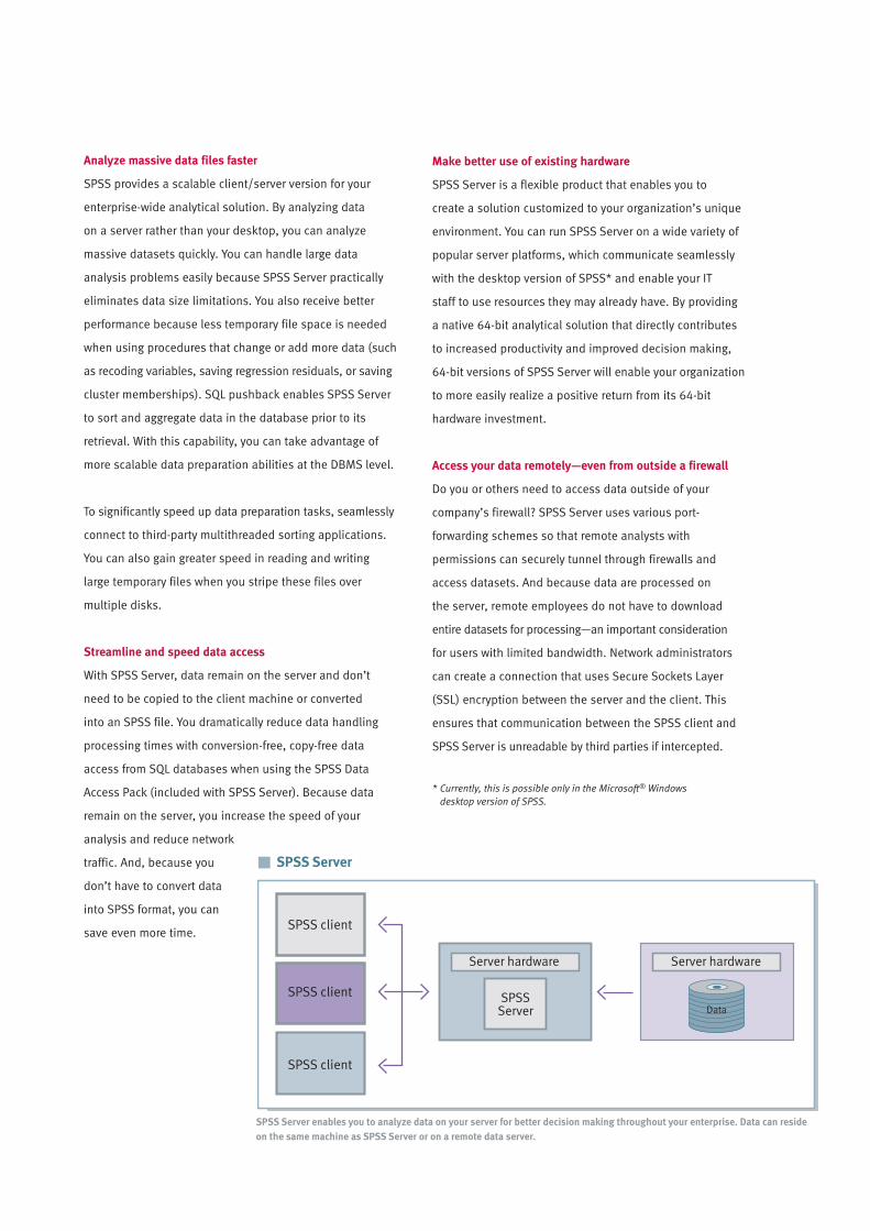
Enterprise productsSPSS ServerSPSS Server enables SPSS users in your
organization to work with large data files
for better decision making. The client/server
version combines SPSS for Windows with
SPSS Server and a wide range of add-on
modules to deliver enterprise-strength
scalability and enhanced performance.
SPSS Adapter for SPSS Predictive Enterprise Services™ Enterprise users gain powerful capabilities to
manage their analytical assets and processes
with the SPSS Adapter. The SPSS Adapter
enables SPSS for Windows to integrate into
the SPSS Predictive Enterprise Services
platform. This enterprise-level application
provides you with a centralized, secure,
auditable repository for data and models.
With it, for example, your organization can:
■ Institutionalize analytics and models
and schedule jobs
■ Standardize the use of SPSS transformations
and models throughout your organization
■ Regularly refresh information for models
and scoring databases
■ Audit analysis conducted for regulatory
compliance
Features subject to change based on final product release. Symbol indicates a new feature. 11
SPSS FamilyAdd more analytical power, as you need it,
with optional add-on modules and stand-alone
software from the SPSS Family. Unless otherwise
noted, the products described below require
you to use the corresponding version of SPSS
Base to operate.
SPSS Programmability Extension™
Expanded programmability functionality
helps make SPSS one of the most powerful
statistical development platforms. You can use
the external programming language Python®
to develop new procedures and applications,
including those written in R. You’ll enjoy
improved tools for adding these procedures,
namely a new user interface and the ability
to deliver results to pivot tables in the SPSS
Output Viewer. Visit SPSS Developer Central
at www.spss.com/devcentral to share code,
tools, and programming ideas.
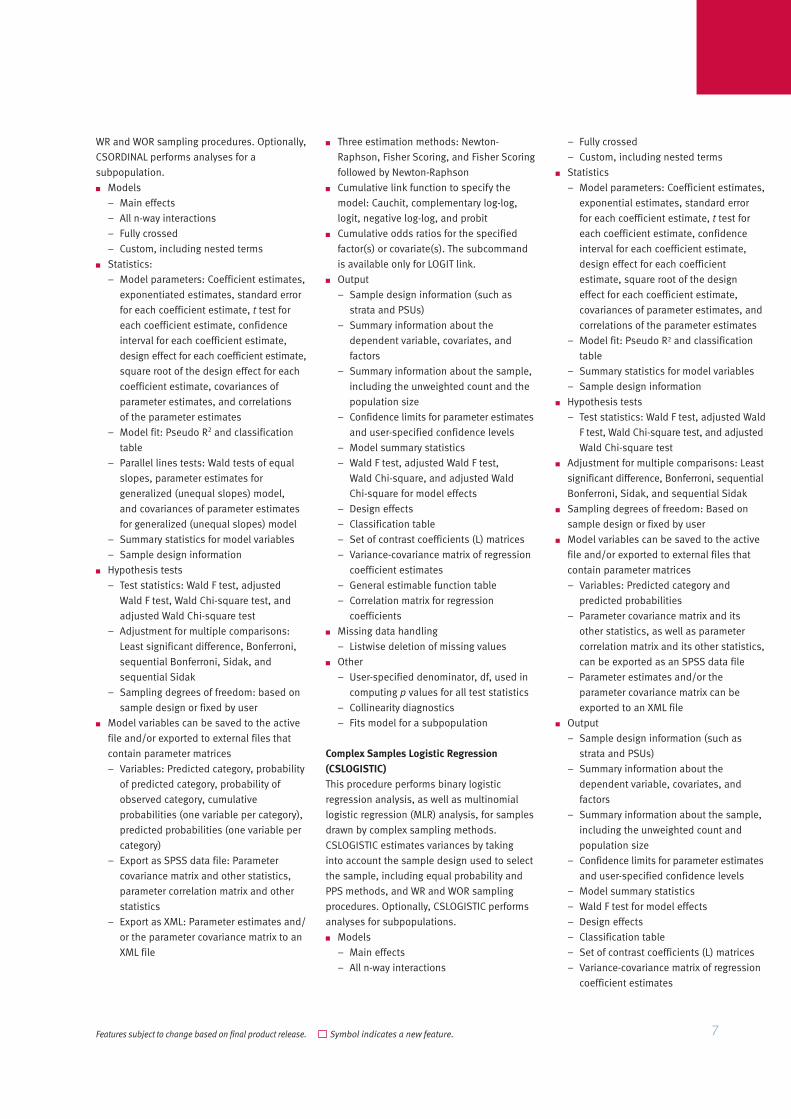
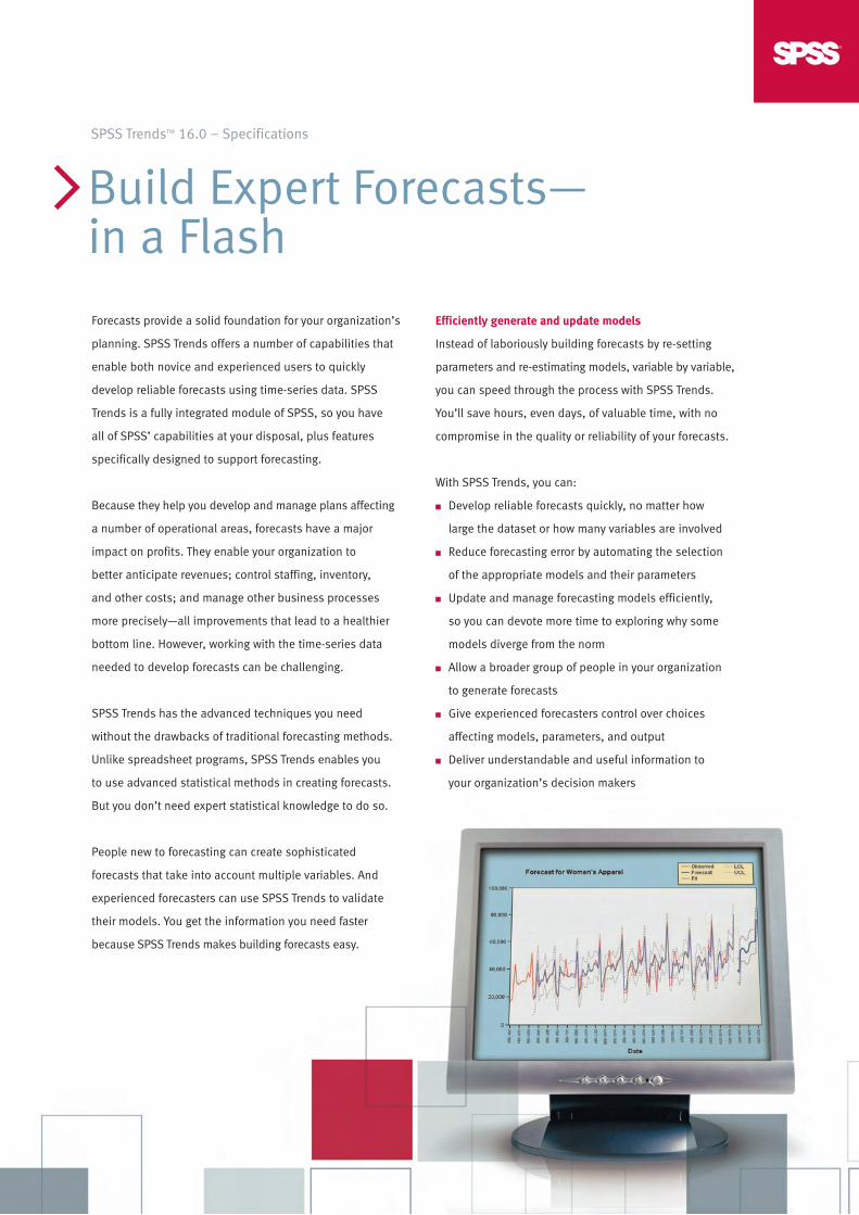
SPSS Regression ModelsPredict behavior or events when your data go
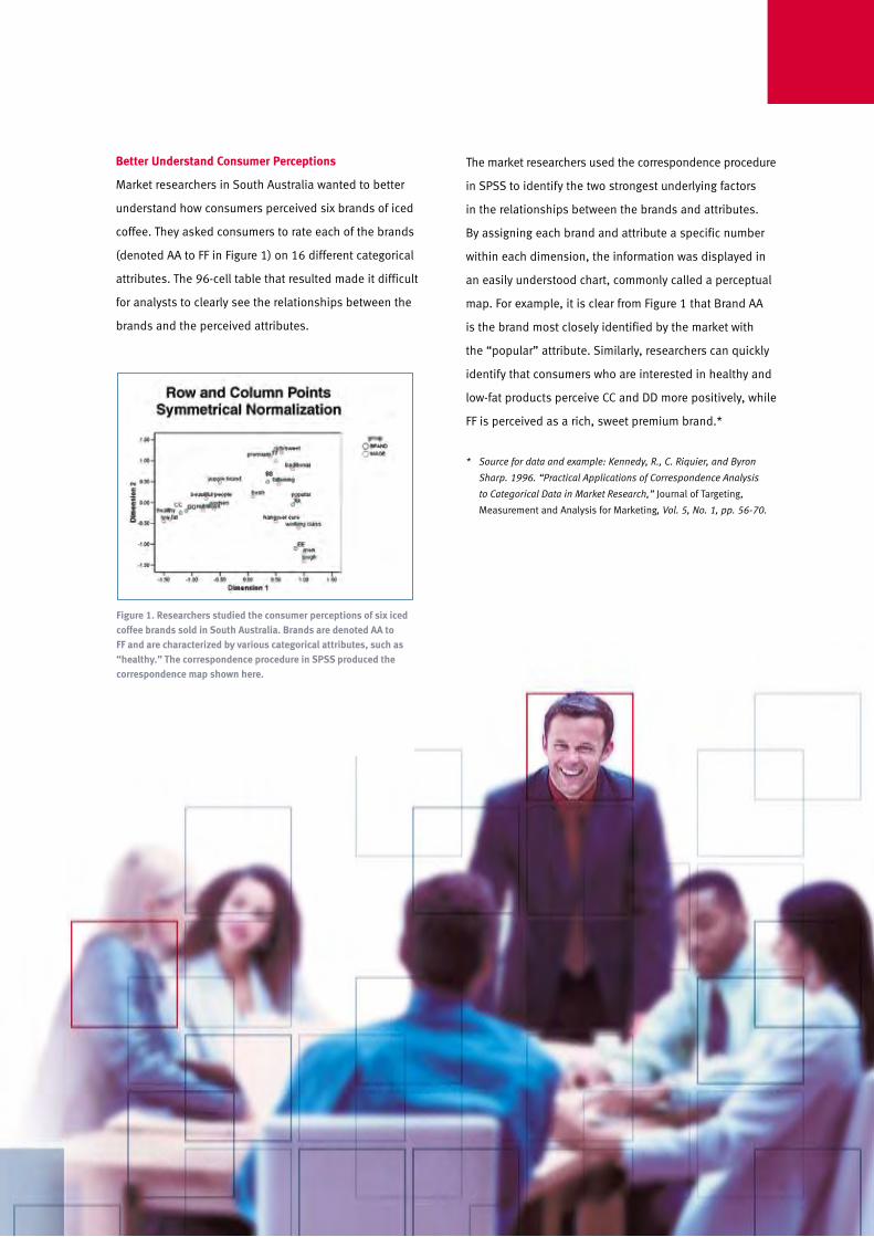
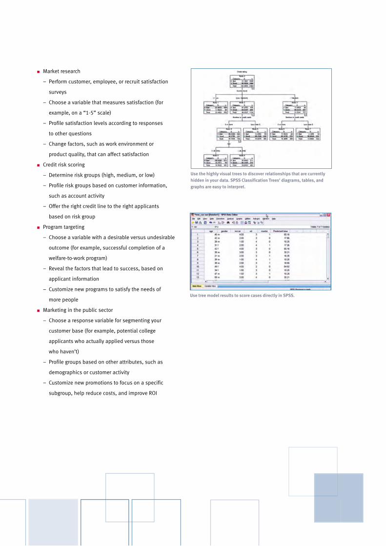
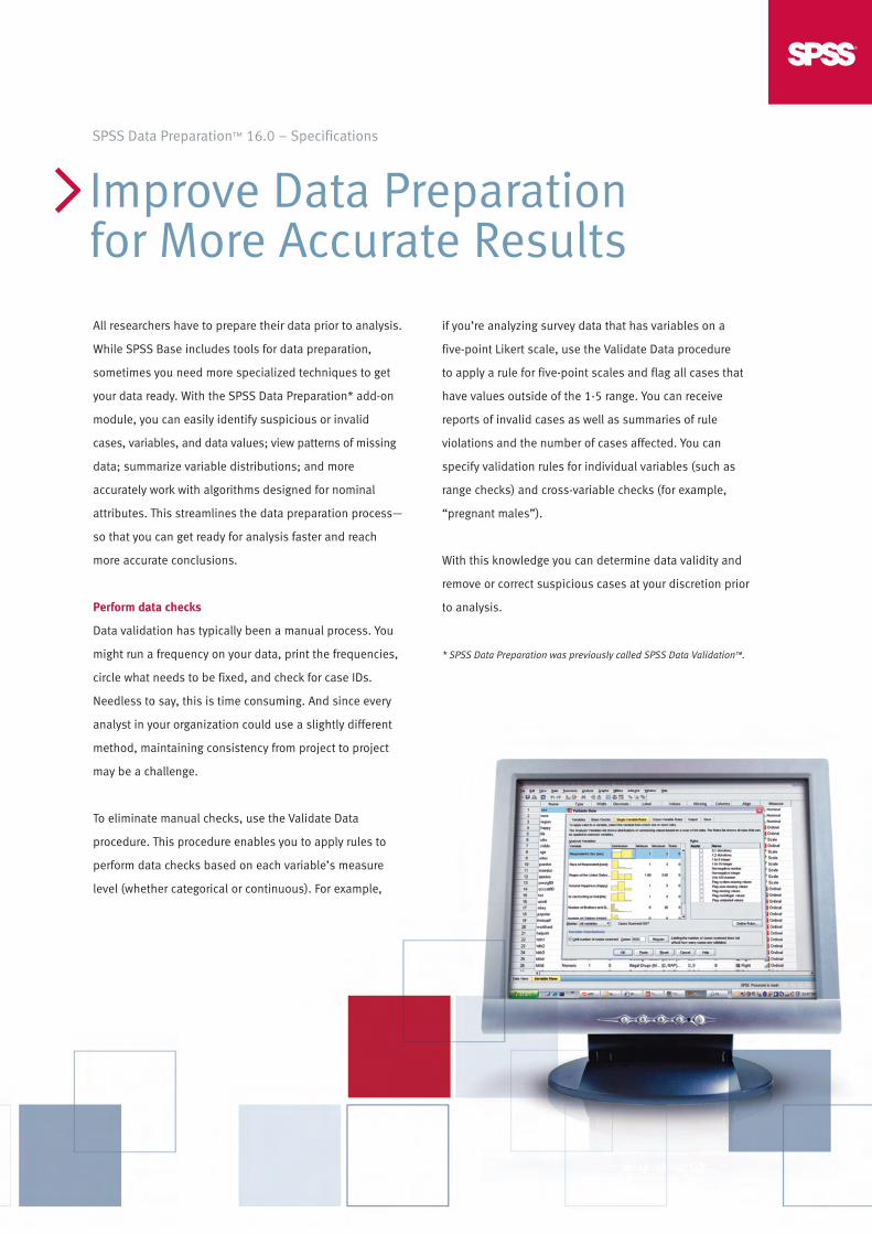
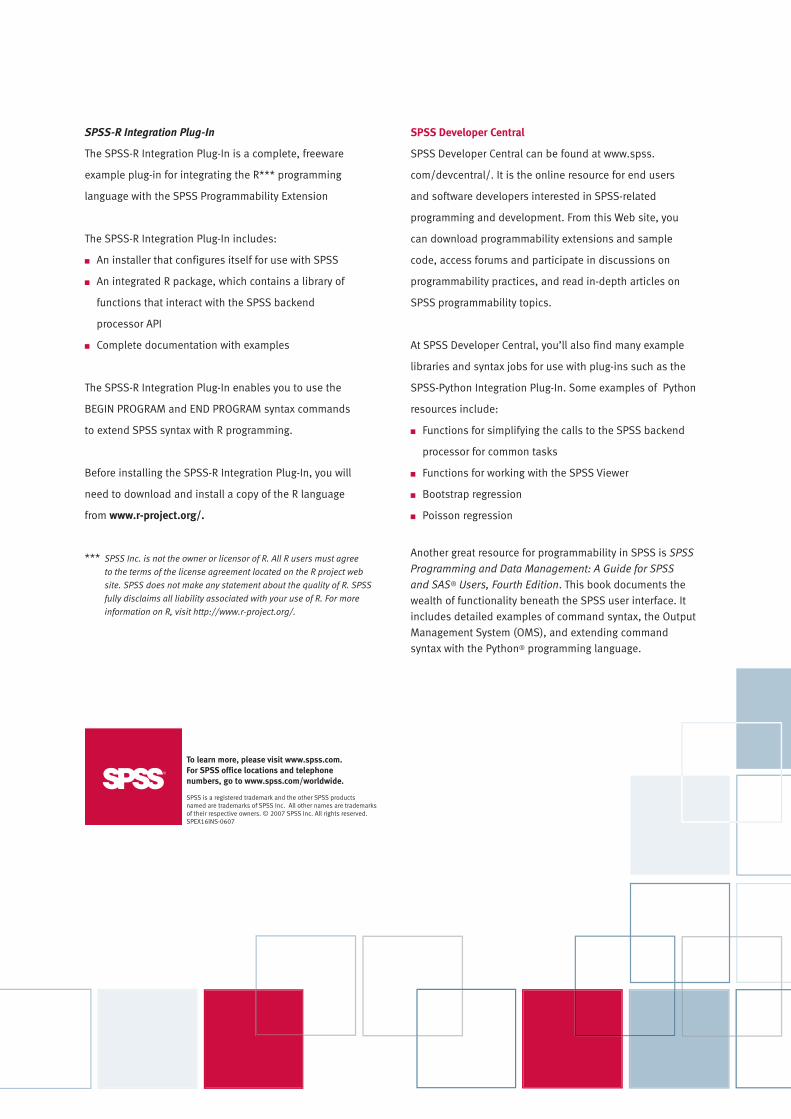
* Source for data and example: Kennedy, R., C. Riquier, and Byron
Sharp. 1996. “Practical Applications of Correspondence Analysis
to Categorical Data in Market Research,” JournalofTargeting,
MeasurementandAnalysisforMarketing, Vol. 5, No. 1, pp. 56-70.
Figure 1. Researchers studied the consumer perceptions of six iced coffee brands sold in South Australia. Brands are denoted AA to FF and are characterized by various categorical attributes, such as “healthy.” The correspondence procedure in SPSS produced the correspondence map shown here.
FeaturesStatisticsCATREG
■ Categoricalregressionanalysisthrough
optimalscaling
– Specifytheoptimalscalinglevelatwhich
youwanttoanalyzeeachvariable.
Choosefrom:Splineordinal(monotonic),
splinenominal(nonmonotonic),ordinal,
nominal,multiplenominal,ornumerical.
– Discretizecontinuousvariablesorconvert
stringvariablestonumericintegervalues
bymultiplying,ranking,orgroupingvalues
intoapreselectednumberofcategories
accordingtoanoptionaldistribution
(normaloruniform),orbygrouping
valuesinapreselectedintervalinto
categories.Therankingandgrouping
optionscanalsobeusedtorecode
categoricaldata.
– Specifyhowyouwanttohandlemissing
data.Imputemissingdatawiththe
variablemodeorwithanextracategory,
oruselistwiseexclusion.
– Specifyobjectstobetreatedas
supplementary
– Specifythemethodusedtocompute
theinitialsolution
– Controlthenumberofiterations
– Specifytheconvergencecriterion
– Plotresults,eitheras:
■ Transformationplots(optimal
categoryquantificationsagainst
categoryindicators)
■ Residualplots
– Addtransformedvariables,predicted
values,andresidualstotheworking
datafile
– Printresults,including:
■ MultipleR,R2,andadjustedR2charts
■ Standardizedregressioncoefficients,
standarderrors,zero-ordercorrelation,
partcorrelation,partialcorrelation,
Pratt’srelativeimportancemeasure
forthetransformedpredictors,tolerance
beforeandaftertransformation,and
Fstatistics
■ Tableofdescriptivestatistics,including
marginalfrequencies,transformation
type,numberofmissingvalues,
andmode
■ Iterationhistory
■ Tablesforfitandmodelparameters:
ANOVAtablewithdegreesoffreedom
accordingtooptimalscalinglevel;
modelsummarytablewithadjusted
R2foroptimalscaling,tvalues,and
significancelevels;aseparatetable
withthezero-order,partandpartial
correlation,andtheimportanceand
tolerancebeforeandaftertransformation
■ Correlationsofthetransformed
predictorsandeigenvaluesofthe
correlationmatrix
■ Correlationsoftheoriginalpredictors
andeigenvaluesofthecorrelation
matrix
■ Categoryquantifications
– Writediscretizedandtransformeddata
toanexternaldatafile
CORRESPONDENCE
■ Correspondenceanalysis
– Inputdataasacasefileordirectlyas
tableinput
– Specifythenumberofdimensionsof
thesolution
– Choosefromtwodistancemeasures:
Chi-squaredistancesforcorrespondence
analysisorEuclideandistancesforbiplot
analysistypes
– Choosefromfivetypesof
standardization:Removerowmeans,
removecolumnmeans,removerow-
and-columnmeans,equalizerowtotals,
orequalizecolumntotals
– Fivetypesofnormalization:Symmetrical,
principal,rowprincipal,column
principal,andcustomized
– Printresults,including:
■ Correspondencetable
■ Summarytable:Singularvalues,
inertia,proportionofinertia
accountedforbythedimensions,
cumulativeproportionofinertia
accountedforbythedimensions,
confidencestatisticsforthemaximum
numberofdimensions,rowprofiles,
andcolumnprofiles
■ Overviewofrowandcolumnpoints:
Mass,scores,inertia,contribution
ofthepointstotheinertiaofthe
dimensions,andcontributionofthe
dimensionstotheinertiaofthepoints
■ Rowandcolumnconfidencestatistics:
Standarddeviationsandcorrelations
foractiverowandcolumnpoints
■ Permutedtable:Tablewithrowsand
columnsorderedbyrowandcolumn
scoresforagivendimension
■ Plotresults:Rowscores,column
scores,andbiplot(jointplotofarow
orcolumnscore)
– Writerowscores,columnscores,and
confidencestatistics(variancesand
covariances)toanexternaldatafile
MULTIPLE CORRESPONDENCE
■ Multiplecorrespondenceanalysis(replaces
HOMALS,whichwasincludedinversions
priortoSPSSCategories13.0)
– Specifyvariableweights
– Discretizecontinuousvariablesor
convertstringvariablestonumeric
integervaluesbymultiplying,ranking,
orgroupingvaluesintoapreselected
numberofcategoriesaccordingtoan
optionaldistribution(normaloruniform),
orbygroupingvaluesinapreselected
intervalintocategories.Theranking
andgroupingoptionscanalsobeused
torecodecategoricaldata.
– Specifyhowyouwanttohandlemissing
data.Excludeonlythecellsofthedata
matrixwithoutvalidvalue,impute
missingdatawiththevariablemodeor
withanextracategory,oruselistwise
exclusion.
– Specifyobjectsandvariablestobe
treatedassupplementary(fulloutputis
includedforcategoriesthatoccuronly
forsupplementaryobjects)
– Specifythenumberofdimensionsin
thesolution
– Specifyafilecontainingthecoordinates
ofaconfigurationandfitvariablesinthis
fixedconfiguration
– Choosefromfivenormalizationoptions:
Variableprincipal(optimizesassociations
betweenvariables),objectprincipal
(optimizesdistancesbetweenobjects),
symmetrical(optimizesrelationships
betweenobjectsandvariables),
independent,orcustomized(user-
specifiedvalueallowinganythingin
betweenvariableprincipalandobject
principalnormalization)
– Controlthenumberofiterations
– Specifyconvergencecriterion
– Printresults,including:
■ Modelsummary
■ Iterationstatisticsandhistory
Features subject to change based on final product release.
■ Descriptivestatistics(frequencies,
missingvalues,andmode)
■ Discriminationmeasuresbyvariable
anddimension
■ Categoryquantifications(centroid
coordinates),mass,inertiaofthe
categories,contributionofthe
categoriestotheinertiaofthe
dimensions,andcontributionof
thedimensionstotheinertiaof
thecategories
■ Correlationsofthetransformed
variablesandtheeigenvaluesofthe
correlationmatrixforeachdimension
■ Correlationsoftheoriginalvariables
andtheeigenvaluesofthecorrelation
matrix
■ Objectscores
■ Objectcontributions:Mass,inertia,
contributionoftheobjectstothe
inertiaofthedimensions,and
contributionofthedimensionsto
theinertiaoftheobjects
– Plotresults,creating:
■ Categoryplots:Categorypoints,
transformation(optimalcategory
quantificationsagainstcategory
indicators),residualsforselected
variables,andjointplotofcategory
pointsforaselectionofvariables
■ Objectscores
■ Discriminationmeasures
■ Biplotsofobjectsandcentroidsof
selectedvariables
– Addtransformedvariablesandobject
scorestotheworkingdatafile
– Writediscretizeddata,transformed
data,andobjectscorestoanexternal
datafile
CATPCA
■ Categoricalprincipalcomponentsanalysis
throughoptimalscaling
– Specifytheoptimalscalinglevelatwhich
youwanttoanalyzeeachvariable.
Choosefrom:Splineordinal(monotonic),
splinenominal(nonmonotonic),ordinal,
nominal,multiplenominal,ornumerical.
– Specifyvariableweights
– Discretizecontinuousvariablesor
convertstringvariablestonumeric
integervaluesbymultiplying,ranking,
orgroupingvaluesintoapreselected
numberofcategoriesaccordingtoan
optionaldistribution(normaloruniform),
orbygroupingvaluesinapreselected
intervalintocategories.Theranking
andgroupingoptionscanalsobeused
torecodecategoricaldata.
– Specifyhowyouwanttohandle
missingdata.Excludeonlythecellsof
thedatamatrixwithoutvalidvalue,
imputemissingdatawiththevariable
modeorwithanextracategory,oruse
listwiseexclusion.
– Specifyobjectsandvariablestobe
treatedassupplementary(fulloutput
isincludedforcategoriesthatoccur
onlyforsupplementaryobjects)
– Specifythenumberofdimensionsin
thesolution
– Specifyafilecontainingthecoordinates
ofaconfigurationandfitvariablesinthis
fixedconfiguration
– Choosefromfivenormalizationoptions:
Variableprincipal(optimizesassociations
betweenvariables),objectprincipal
(optimizesdistancesbetweenobjects),
symmetrical(optimizesrelationships
betweenobjectsandvariables),
independent,orcustomized(user-
specifiedvalueallowinganythingin
betweenvariableprincipalandobject
principalnormalization)
– Controlthenumberofiterations
– Specifyconvergencecriterion
– Printresults,including:
■ Modelsummary
■ Iterationstatisticsandhistory
■ Descriptivestatistics(frequencies,
missingvalues,andmode)
■ Varianceaccountedforbyvariable
anddimension
■ Componentloadings
■ Categoryquantificationsandcategory
coordinates(vectorand/orcentroid
coordinates)foreachdimension
■ Correlationsofthetransformed
variablesandtheeigenvaluesof
thecorrelationmatrix
■ Correlationsoftheoriginalvariables
andtheeigenvaluesofthecorrelation
matrix
■ Object(component)scores
– Plotresults,creating:
■ Categoryplots:Categorypoints,
transformations(optimalcategory
quantificationsagainstcategory
indicators),residualsforselected
variables,andjointplotofcategory
pointsforaselectionofvariables
■ Plotoftheobject(component)scores
■ Plotofcomponentloadings
PREFSCAL (syntax only)
■ Visuallyexaminerelationshipsbetween
variablesintwosetsofobjectsinorderto
findacommonquantitativescale
– Readoneormorerectangularmatrices
ofproximities
– Readweights,initialconfigurations,
andfixedcoordinates
– Optionallytransformproximitieswith
linear,ordinal,smoothordinal,orspline
functions
– Specifymultidimensionalunfolding
withidentity,weightedEuclidean,or
generalizedEuclideanmodels
– Specifyfixedrowandcolumn
coordinatestorestricttheconfiguration
– Specifyinitialconfiguration(classical
triangle,classicalSpearman,Ross-Cliff,
correspondence,centroids,random
starts,orcustom),iterationcriteria,
andpenaltyparameters
– Specifyplotsformultiplestarts,initial
commonspace,stressperdimension,
finalcommonspace,spaceweights,
individualspaces,scatterplotoffit,
residualsplot,transformationplots,
andShepardplots
– Specifyoutputthatincludestheinput
data,multiplestarts,initialcommon
space,iterationhistory,fitmeasures,
stressdecomposition,finalcommon
space,spaceweights,individual
spaces,fitteddistances,and
transformedproximities
– Writecommonspacecoordinates,
individualweights,distances,and
transformedproximitiestoafile
System requirements ■ Software:SPSSBase16.0
■ Othersystemrequirementsvary
accordingtoplatformTo learn more, please visit www.spss.com. For SPSS office locations and telephone numbers, go to www.spss.com/worldwide.
Highly visual diagrams enable you to present categorical
results in an intuitive manner—so you can more clearly
explain categorical results to non-technical audiences.
These trees enable you to explore your results and
visually determine how your model flows. Visual results
can help you find specific subgroups and relationships
that you might not uncover using more traditional
statistics. Because classification trees break the data
down into branches and nodes, you can easily see where
a group splits and terminates.
Use SPSS Classification Trees in a variety of applications,
including:
n Database marketing
– Choose a response variable to segment your customer
base (for example, responders/non-responders in a
test mailing; high-, medium-, and low-profit customers;
or recruits who have extended service versus those
who haven’t)
– Profile groups based on other attributes, such as
demographics or customer activity
– Customize new promotions to focus on a specific
subgroup, help reduce costs, and improve return
on investment (ROI)
n Market research
– Perform customer, employee, or recruit satisfaction
surveys
– Choose a variable that measures satisfaction (for
example, on a “1-5” scale)
– Profile satisfaction levels according to responses
to other questions
– Change factors, such as work environment or
product quality, that can affect satisfaction
n Credit risk scoring
– Determine risk groups (high, medium, or low)
– Profile risk groups based on customer information,
such as account activity
– Offer the right credit line to the right applicants
based on risk group
n Program targeting
– Choose a variable with a desirable versus undesirable
outcome (for example, successful completion of a
welfare-to-work program)
– Reveal the factors that lead to success, based on
applicant information
– Customize new programs to satisfy the needs of
more people
n Marketing in the public sector
– Choose a response variable for segmenting your
customer base (for example, potential college
applicants who actually applied versus those
who haven’t)
– Profile groups based on other attributes, such as
demographics or customer activity
– Customize new promotions to focus on a specific
subgroup, help reduce costs, and improve ROI
Use the highly visual trees to discover relationships that are currently hidden in your data. SPSS Classification Trees’ diagrams, tables, and graphs are easy to interpret.
Use tree model results to score cases directly in SPSS.
Choose from four decision tree algorithms
SPSS Classification Trees includes four established tree-
growing algorithms:
n CHAID—A fast, statistical, multi-way tree algorithm
that explores data quickly and efficiently, and builds
segments and profiles with respect to the desired
outcome
n Exhaustive CHAID—A modification of CHAID that
examines all possible splits for each predictor
n Classification & regression trees (C&RT)—A complete
binary tree algorithm that partitions data and
produces accurate homogeneous subsets
n QUEST—A statistical algorithm that selects variables
without bias and builds accurate binary trees quickly
and efficiently
With four algorithms, you have the ability to try different
tree-growing methods and find the one that best fits
your data.
Extend your results with further analysis within SPSS
Since you use SPSS Classification Trees within the SPSS
interface, you can create classification trees directly in
SPSS and conveniently use the results to segment and
group cases directly within the data. There is no back
and forth between SPSS and other software. Additionally,
you can generate selection or classification/prediction
rules in the form of SPSS syntax, SQL statements, or
simple text (through syntax). You can display these rules
in the Viewer and save them to an external file for later
use to make predictions about individual and new cases.
If you’d like to use your results to score other data files,
you can write information from the tree model directly to
your data or create XML models for use in SPSS Server.
Create tree models in SPSS using CHAID, Exhaustive CHAID, C&RT, or QUEST.
Directly select cases or assign predictions in SPSS from the model results, or export rules for later use.
FeaturesTreesn Display tree diagrams, tree maps, bar
graphs, and data tables
n Easily build trees using the comprehensive
interface, which enables the setup of:
– Measurement level (nominal, ordinal,
and continuous)
– Independent variables
– Dependent variables
– Influence variables
– Growing method
– Output setup, which includes trees,
statistics, charts, and rules
– Split sample validation or cross-validation
– Stopping criteria
– Saved variables, including predicted
values, probability, and XML models
n Choose from four tree-growing methods
n View nodes using one of several methods:
Show bar charts or tables of your target
variables, or both, in each node
n Collapse and expand branches, and change
other cosmetic properties, such as fonts
and colors
n View and print trees
n Specify the exact zoom percentage for
viewing visual tree models in the interface
n Automate tree building using the
production mode
– Automatically generate syntax from
the interface
n Force one predictor into the model
n Specify prior probabilities, misclassifica-
tion costs, revenues, expenses, and scale
scores
Tree-growing algorithmsn Perform analysis using one of four powerful
tree-growing algorithms:
– CHAID by Kass (1980)
– Exhaustive CHAID by Biggs, de Ville,
and Suen (1991)
– Classification & regression trees (C&RT)
by Breiman, Friedman, Olshen, and
Stone (1984)
– QUEST by Loh and Shih (1997)
n Handle missing predictor data using one
of two methods: Assign to a category or
impute using a surrogate
n Discretize continuous predictor variables
according to the number of categories
specified
n Have pruning capabilities for C&RT and
QUEST
n Randomly sample source data for split
sample validation or use a variable to split
the sample
Model evaluationn Generate risk and classification tables
n Summarize node performance with
evaluation graphs and tables to help
identify the best segments:
– Gains
– Index (lift)
– Response
– Mean
– Average profit
– ROI
n Partition data between training and test
data to verify accuracy
n Display summary graphs or classification
rules for selected nodes using the node
summary window
Deploymentn Export:
– Tree diagrams, charts, and tables.
Export formats include: HTML, text,
Word/RTF, and Excel® files, and PDF
n Save information from the model as
variables in the working data file
n Export decision rules that define selected
segments in SQL to score databases, as
SPSS syntax to score SPSS files, or as
simple text (through syntax)
n Export trees as XML models for use with
SPSS Server and SmartScore® to score new
cases or data files
n Publish trees as images and tables as static
or interactive tables to SmartViewer® Web
Server™
n For additional insight, select interesting
segments in the working data file via tree
nodes, and run more analyses
System requirementsn Software: SPSS Base 16.0
n Other system requirements vary according
to platform
To learn more, please visit www.spss.com. For SPSS office locations and telephone numbers, go to www.spss.com/worldwide.
specialized statistics that enable you to correctly and
easily compute statistics and their standard errors from
complex sample designs. You can apply it to:
n Survey research—Obtain descriptive and inferential
statistics for survey data
n Market research—Analyze customer satisfaction data
n Health research—Analyze large public-use datasets
on public health topics such as health and nutrition
or alcohol use and traffic fatalities
n Social science—Conduct secondary research on
public survey datasets
n Public opinion research—Characterize attitudes on
policy issues
SPSS Complex Samples provides you with everything you
need for working with complex samples. It includes:
n An intuitive Sampling Wizard that guides you step by
step through the process of designing a scheme and
drawing a sample
n An easy-to-use Analysis Preparation Wizard to help
prepare public-use datasets that have been sampled,
such as the National Health Inventory Survey data from
the Centers for Disease Control and Prevention (CDC)
n Numerical outcome prediction through the Complex
Samples General Linear Model (CSGLM)
n Ordinal outcome prediction through Complex Samples
Ordinal Regression (CSORDINAL)
n Categorical outcome prediction through Complex
Samples Logistic Regression (CSLOGISTIC)
n Time to an event prediction through Complex Samples
Cox Regression (CSCOXREG)
From the planning stage and sampling through the analysis
stage, SPSS Complex Samples makes it easy to obtain
accurate and reliable results. Since SPSS Complex Samples
takes up to three states into account when analyzing
data from a multistage design, you’ll end up with more
accurate analyses. In addition to giving you the ability to
assess your design’s impact, SPSS Complex Samples also
produces a more accurate picture of your data because
subpopulation assessments take other subpopulations
into account.
You can use the following types of sample design
information with SPSS Complex Samples:
n Stratified sampling—Increase the precision of your
sample or ensure a representative sample from key
groups by choosing to sample within subgroups of
the survey population. For example, subgroups
might be a specific number of males or females, or
contain people in certain job categories or people of
a certain age group.
n Clustered sampling—Select clusters, which are groups
of sampling units, for your survey. Clusters can include
schools, hospitals, or geographic areas with sampling
units that might be students, patients, or citizens.
Clustering often helps make surveys more cost-effective.
n Multistage sampling—Select an initial or first-stage
sample based on groups of elements in the population,
then create a second-stage sample by drawing a
subsample from each selected unit in the first-stage
sample. By repeating this option, you can select a
higher-stage sample.
More confidently reach results
As a researcher, you want to be confident about your
results. Most conventional statistical software assumes
your data arise from simple random sampling. Simple
random sampling, however, is generally neither feasible
nor cost-effective in most large-scale surveys. Analyzing
such sample data with conventional statistics risks
incorrect results. For example, estimated standard errors
of statistics are often too small, giving you a false sense
of precision. SPSS Complex Samples enables you to
achieve more statistically valid inferences for populations
measured in your complex sample data because it
incorporates the sample design into survey analysis.
Work efficiently and easily
Only SPSS Complex Samples makes understanding and
working with your complex sample survey results easy.
Through the intuitive interface, you can analyze data and
interpret results. When you’re finished, you can publish
datasets and include your sampling or analysis plans.
Each plan acts as a template and allows you to save all
the decisions made when creating it. This saves time and
improves accuracy for yourself and others who may want
to use your plans with the data, either to replicate results
or pick up where you left off.
A grocery store wants to determine if the frequency with which customers shop is related to the amount spent, controlling for gender of the customer and incorporating a sample design. First, the store specifies the sample design used in the Analysis Preparation Wizard (top). Next, the store sets up the model in the Complex Samples General Linear Model (bottom).
2
To begin your work in SPSS Complex Samples, use the
wizards, which prompt you for the many factors you must
consider. If you are creating your own samples, use the
Sampling Wizard to define the sampling scheme. If you’re
using public-use datasets that have been sampled, such
as those provided by the CDC, use the Analysis Preparation
Wizard to specify how the samples were defined and how
to estimate standard errors. Once you create a sample or
specify standard errors, you can create plans, analyze
your data, and produce results (see the diagram above
for workflow).
SPSS Complex Samples makes it easy to learn and work
quickly. Use the online help system, explore the interactive
case studies, or run the online tutorial to learn more about
using your data with the software. SPSS Complex Samples
enables you to:
n Reach correct point estimates for statistics such as
totals, means, and ratios
n Obtain the standard errors of these statistics
n Produce correct confidence intervals and hypothesis tests
n Predict numerical outcomes
n Predict ordinal outcomes
n Predict categorical outcomes
n Predict time to an event
Accurate analysis of survey data is easy in SPSS Complex Samples. Start with one of the wizards (which one to select depends on your data source) and then use the interactive interface to create plans, analyze data, and interpret results.
3
FeaturesComplex Samples Plan (CSPLAN)This procedure provides a common place
to specify the sampling frame to create
a complex sample design or analysis
specification used by companion procedures
in the SPSS Complex Samples add-on
module. CSPLAN does not actually extract
the sample or analyze data. To sample cases,
use a sample design created by CSPLAN as
input to the CSSELECT procedure (described
on the next page). To analyze sample data,
use an analysis design created by CSPLAN
as input to the CSDESCRIPTIVES, CSTABULATE,
CSGLM, CSLOGISTIC, or CSORDINAL procedures
(described on the following pages).
n Create a sample design: Use to extract
sampling units from the active file
n Create an analysis design: Use to analyze
a complex sample
n When you create a sample design, the
procedure automatically saves an
appropriate analysis design to the plan
file. A plan file is created for designing a
sample, and therefore, can be used for
both sample selection and analysis.
n Display a sample design or analysis design
n Specify the plan in an external file
n Name planwise variables to be created
when you extract a sample or use it as
input to the selection or estimation
process with the PLANVARS subcommand
– Specify final sample weights for each
unit to be used by SPSS Complex
Samples analysis procedures in the
estimation process
– Indicate overall sample weights that will
be generated when the sample design
is executed in the CSSELECT procedure
– Select weights to be used when
computing final sampling weights in
a multistage design
n Control output from the CSPLAN procedure
with the PRINT subcommand
– Display a plan specifications summary
in which the output reflects your
specifications at each stage of the design
– Display a table showing MATRIX
specifications
n Signal stages of the design with the
DESIGN subcommand. You can also use
this subcommand to define stratification
variables and cluster variables or create
descriptive labels for particular stages.
n Specify the sample extraction method using
the METHOD subcommand. Select from a
variety of equal- and unequal-probability
methods, including simple and systematic
random sampling. Methods for sampling
with probability proportionate to size (PPS)
are also available. Units can be drawn with
replacement (WR) or without replacement
(WOR) from the population.
– SIMPLE_WOR: Select units with equal
probability. Extract units without
replacement.
– SIMPLE_WR: Select units with equal
probability. Extract units with
replacement.
– SIMPLE_SYSTEMATIC: Select units at
a fixed interval throughout the sampling
frame or stratum. A random starting
point is chosen within the first interval.
– SIMPLE_CHROMY: Select units
sequentially with equal probability.
Extract units without replacement.
– PPS_WOR: Select units with probability
proportional to size. Extract units without
replacement.
– PPS_WR: Select units with probability
proportional to size. Extract units with
replacement.
– PPS_SYSTEMATIC: Select units by
systematic random sampling with
probability proportional to size.
Extract units without replacement.
– PPS_CHROMY: Select units sequentially
with probability proportional to size.
Extract units without replacement.
– PPS_BREWER: Select two units from each
stratum with probability proportional to
size. Extract units without replacement.
– PPS_MURTHY: Select two units from each
stratum with probability proportional to
size. Extract units without replacement.
– PPS_SAMPFORD: Extends Brewer’s
method to select more than two units
from each stratum with probability
proportional to size. Extract units
without replacement.
– Control for the number or percentage of
units to be drawn: Set at each stage of
the design. You can also choose output
variables, such as stagewise sampling
weights, which are created upon the
sample design execution.
– Estimation methods: With replacement,
equal probability without replacement
in the first stage, and unequal probability
without replacement
– You can choose whether to include the
finite population correction when
estimating the variance under simple
random sampling (SRS)
– Unequal probability estimation without
replacement: Request in the first stage
only
– Variable specification: Specify variables
for input for the estimation process,
including overall sample weights and
inclusion probabilities
n Specify the number of sampling units
drawn at the current stage using the SIZE
subcommand
n Specify the percentage of units drawn at
the current stage. For example, specify
the sampling fraction using the RATE
subcommand.
n Specify the minimum number of units drawn
when you specify RATE. This is useful when
the sampling rate for a particular stratum is
very small due to rounding.
n Specify the maximum number of units to
draw when you specify RATE. This is
useful when the sampling rate for a
particular stratum is larger than desired
due to rounding.
n Specify the measure of size for population
units in a PPS design. Specify a variable
that contains the sizes or request that
sizes be determined when the CSSELECT
procedure scans the sample frame.
n Obtain stagewise sample information
variables when you execute a sample
design using the STAGEVARS subcommand.
You can obtain:
– The proportion of units drawn from
the population at a particular stage
using stagewise inclusion (selection)
probabilities
– Prior stages using cumulative sampling
weight for a given stage
– Uniquely identified units that have been
selected more than once when your
sample is done with replacement, with
a duplication index for units selected in
a given stage
– Population size for a given stage
– Number of units drawn at a given stage
– Stagewise sampling rate
– Sampling weight for a given stage
Features subject to change based on final product release. Symbol indicates a new feature.4
In the real world, buyers do not make decisions based on
a single attribute, such as price or brand name. Instead,
they examine a range of products, all with different
combinations of features and attributes, and perform a
complex series of trade-offs before reaching a decision.
Conjoint analysis is the research tool used to model the
consumer’s decision-making process. Using SPSS Conjoint
can increase your understanding of consumer preferences,
enabling you to more effectively design, price, and market
successful products.
Conjoint analysis enables you to measure the value
consumers place on individual attributes or features that
define products and services. Armed with this knowledge,
your company can design products that include the features
most important to your target market, set prices based on
the value the market assigns to the product’s attributes,
and focus messages on the points most likely to appeal to
target buyers.
Even as competitors, products, and pricing change over
time in the market, you can continue to use the results
from SPSS Conjoint to develop market simulation models
that incorporate changes, along with your proposed
responses. This enables you to predict the response to
your proposed actions before spending valuable resources
on product development and marketing programs.
SPSS Conjoint provides answers to your critical questions
n Which features or attributes of a product or service
drive the purchase decision?
n Which feature combinations will have the most success?
n What market segment is most interested in the product?
n What marketing messages will most appeal to that
segment?
n What feature upgrades will most affect consumer
preference and increase sales?
n What is the optimal price to charge consumers for a
product or service?
n Can the price be increased without a significant loss
in sales?
n Are product levels too close together?
SPSS Conjoint gives you all the tools you need
The three procedures in SPSS Conjoint enable you to plan,
implement, and efficiently analyze results from conjoint
studies. Following is a summary of these procedures.
n Generate designs easily — Orthoplan produces an
orthogonal array of product attribute combinations,
which dramatically reduces the number of questions
you must ask while ensuring that you have enough
information to perform a full analysis
n Print “cards” to elicit respondents’ preferences —
Plancards quickly generates cards that respondents
can use to easily sort and rank product attribute
combinations
n Get informative results — The conjoint procedure
performs a specially tailored version of regression on
your response rankings. You’ll receive results you can
act on, such as which product attributes are important
and at what levels consumers most prefer them. You
can also perform simulations to determine the market
share of preference for any combination of attributes.
Four ways to make your product launch a success
1. Right product — Design your product with the feature
set for which the market has the greatest need
2. Right price — Price your product based on the value
your target audience assigns to it
3. Right place — Predict how your product/price combination
will perform in the market before committing valuable
development and launch resources
4. Right promotion — Focus your marketing on the individual
features that most interest your target audience
Offer options consumers prefer: A real-life study
A software company planned to develop training programs
that differed from its traditional instructor-led training.
Since many options were available, the company decided
to perform a conjoint study to evaluate the proposed
product. The company believed six key attributes would
influence consumer preference: method of delivery,
video content, example types, certification test, method
of asking questions remotely, and price. Four of these
attributes had two levels, while two others had three.
The resulting full factorial design would have had 144
alternative product bundles (2x2x2x2x3x3), making for
an unfeasibly large study. Using orthoplan, the research
department reduced the number of hypothetical product
bundles (such as those shown in Figure 1) to 16, while
ensuring that the department received all the information
needed to perform a complete analysis. A researcher then
printed the 16 product bundles using plancards and gave
them to a sample of target users who ranked them
in order of preference.
A researcher analyzed the preference rankings with
SPSS Conjoint, and the results are shown in Figure 2.
Two attributes stand out as very important—inclusion
of video and price—while test and example types are
relatively unimportant. The Utility Estimate and Standard
Error columns in Figure 2 show the relative preference
for each level of each attribute. Within question, Instant
Message is the most preferred attribute level and No
Support is the least preferred.
Figure 2: Easily identify the attributes a group of consumers prefers.
Figure 1. Save time and money with SPSS Conjoint by using orthoplan to present a fraction of all possible product bundles. Here, orthoplan generates a 16-run orthogonal array instead of all 144 possible combinations.
To learn more, please visit www.spss.com. For SPSS office locations and telephone numbers, go to www.spss.com/worldwide.
Missing data (top left) can leave you with invalid or erroneous results. Mean substitution (top right) and a fairly simple regression (bottom left) show that these methods provide an inaccurate or insignificant way to impute missing values. SPSS Missing Value Analysis (bottom right) provides the best method for imputing missing values. As shown here, it provides a scatterplot of YMISS and Y with imputed missing values.
New Tools for Building Predictive Models
SPSS Neural Networks™ 16.0 – Specifications
Your organization needs to find patterns and connections
in the complex and fast-changing environment you work in
so that you can make better decisions at every turn. You
may be using SPSS and one or more of its add-on modules
to help you do this. If so, you know the power and versatil-
ity you have at your fingertips. But there’s even more you
can do.
You can explore subtle or hidden patterns in your data,
using SPSS Neural Networks. This new add-on module
offers you the ability to discover more complex
relationships in your data and generate better performing
predictive models. The result? Deeper insight and better
decision-making.
The procedures in SPSS Neural Networks complement the
more traditional statistics in SPSS Base and its modules.
Find new associations in your data with SPSS Neural
Networks and then confirm their significance with
traditional statistical techniques.
Why use a neural network?
A computational neural network is a set of non-linear
data modeling tools consisting of input and output layers
plus one or two hidden layers. The connections between
neurons in each layer have associated weights, which are
iteratively adjusted by the training algorithm to minimize
error and provide accurate predictions. You set the
conditions under which the network “learns” and can
finely control the training stopping rules and network
architecture, or let the procedure automatically choose
the architecture for you.
You can combine SPSS Neural Networks with other statistical
procedures to gain clearer insight in a number of areas.
In market research, for example, you can create customer
profiles and discover customer preferences. In database
marketing, you can segment your customer base and
optimize marketing campaigns.
In financial analysis, you can use SPSS Neural Networks
to analyze applicants’ creditworthiness and to detect
possible fraud. In operational analysis, use this new tool
to manage cash flow and improve logistics planning.
Scientific and healthcare applications include forecasting
treatment costs, performing medical outcomes analysis,
and predicting the length of a hospital stay.
Control the process from start to finish
With SPSS Neural Networks, you select either the Multilayer
Perceptron (MLP) or Radial Basis Function (RBF) procedure.
Both of these are supervised learning techniques—that is,
they map relationships implied by the data. Both use feed-
forward architectures, meaning that data moves in only one
direction, from the input nodes through the hidden layer
of nodes to the output nodes. Your choice of procedure will
be influenced by the type of data you have and the level of
complexity you seek to uncover. While the MLP procedure
can find more complex relationships, the RBF procedure is
generally faster.
With either of these approaches, you divide your data into
training, testing, and holdout sets. The training set is used
to estimate the network parameters. The testing set is
used to prevent overtraining. The holdout set is used to
independently assess the final network, which is applied
to the entire dataset and to any new data.
You specify the dependent variables, which may be scale,
categorical, or a combination of the two. If a dependent
variable has scale measurement level, then the neural
network predicts continuous values that approximate the
“true” value of some continuous function of the input
data. If a dependent variable is categorical, then the neural
network is used to classify cases into the “best” category
based on the input predictors.
You adjust the procedure by choosing how to partition
the dataset, what sort of architecture you want, and what
computation resources will be applied to the analysis.
Finally, you choose to display results in tables or graphs,
save optional temporary variables to the active dataset,
and export models in XML-file formats to score future data.
In an MLP network like the one shown here, the data feeds forward from the input layer through one or more hidden layers to the output layer.
The results of exploring data with neural network techniques can be shown in a variety of graphic formats. This simple bar chart is one of many options.
From the Multilayer Perceptron (MLP) dialog, you select the variables that you want to include in your model.
FeaturesMultilayer Perceptron (MLP)The MLP procedure fits a particular kind of
neural network called a multilayer perceptron.
The multilayer perceptron is a supervised
method using feedforward architecture. It can
have multiple hidden layers. One or more
dependent variables may be specified, which
may be scale, categorical, or a combination. If
a dependent variable has scale measurement
level, then the neural network predicts
continuous values that approximate the “true”
value of some continuous function of the input
data. If a dependent variable is categorical,
then the neural network is used to classify
cases into the “best” category based on the
input predictors.
n Predictors
– Factors
– Covariates
n The EXCEPT subcommand lists any variables
that the MLP procedure should exclude
from the factor or covariate lists on the
command line. This subcommand is useful
if the factor or covariate lists contain a large
number of variables.
n The RESCALE subcommand is used to
rescale covariates or scale dependent
variables
– Dependent variable (if scale):
standardized, normalized, adjusted
normalized, or none
– Covariates: standardized, normalized,
adjusted normalized, or none
n The PARTITION subcommand specifies the
method of partitioning the active dataset
into training, testing, and holdout samples.
The training sample comprises the data
records used to train the neural network.
The testing sample is an independent set
of data records used to track prediction
error during training in order to prevent
overtraining. The holdout sample is another
independent set of data records used to
assess the final neural network. You can
specify:
– The relative number of cases in the
active dataset to randomly assign to
the training sample
– The relative number of cases in the
active dataset to randomly assign to
the testing sample
– The relative number of cases in the
active dataset to randomly assign to
the holdout sample
– A variable that assigns each case in
the active dataset to the training, testing,
or holdout sample
n The ARCHITECTURE subcommand is used
to specify the neural network architecture.
You can specify:
– Whether to use the automatic
architecture or, if automatic is not used:
– The number of hidden layers in the
neural network
– The activation function to use for all
units in the hidden layers (Hyperbolic
tangent or Sigmoid)
– The activation function to use for all
units in the output layer (Identity,
Hyperbolic tangent, Sigmoid, or Softmax
n The CRITERIA subcommand specifies the
computational and resource settings for
the MLP procedure. You can specify the
training type, which determines how the
neural network processes training data
records: batch training, online training,
mini-batch training. You can also specify:
– The number of training records per
mini-batch (if selected as the training
method)
– The maximum number of cases to store
in memory when automatic architecture
selection and/or mini-batch training is
in effect
– The optimization algorithm used to
determine the synaptic weights: Gradient
descent, Scaled conjugate gradient
– The initial learning rate for the gradient
descent optimization algorithm
– The lower boundary for the learning rate
when gradient descent is used with
online or mini-batch training
– The momentum rate for the gradient
descent optimization algorithm
– The initial lambda, for the scaled
conjugate gradient optimization
algorithm
– The initial sigma, for the scaled
conjugate gradient optimization
algorithm
– The interval [a0−a, a0+a] in which weight
vectors are randomly generated when
simulated annealing is used
n The STOPPINGRULES subcommand specifies
the rules that determine when to stop
training the neural network. You can specify:
– The number of steps n to allow before
checking for a decrease in prediction error
– Whether the training timer is turned on
or off and the maximum training time
– The maximum number of epochs allowed
– The relative change in training error criterion
– The training error ratio criterion
n The MISSING subcommand is used to
control whether user-missing values for
categorical variables—that is, factors
and categorical dependent variables—
are treated as valid values
n The PRINT subcommand indicates the
tabular output to display and can be
used to request a sensitivity analysis.
You can choose to display:
– The case processing summary table
– Information about the neural network,
including the dependent variables,
number of input and output units,
number of hidden layers and units,
and activation functions
– A summary of the neural network results,
including the average overall error, the
stopping rule used to stop training and
the training time
– A classification table for each categorical
dependent variable
– The synaptic weights; that is, the
coefficient estimates, from layer i−1
unit j to layer i unit k
– A sensitivity analysis, which computes
the importance of each predictor in
determining the neural network
n The PLOT subcommand indicates the chart
output to display. You can display:
– Network diagram
– A predicted by observed value chart for
each dependent variable
– A residual by predicted value chart for
each scale dependent variable
– ROC (Receiver Operating Characteristic)
curves for each categorical dependent
variable. It also displays a table giving
the area under each curve.
– Cumulative gains charts for each
categorical dependent variable
– Lift charts for each categorical dependent
variable
n The SAVE subcommand writes optional
temporary variables to the active dataset.
You can save:
– Predicted value or category
– Predicted pseudo-probability
n The OUTFILE subcommand saves XML-
format files containing the synaptic weights
Radial Basis Function (RBF)The RBF procedure fits a radial basis function
neural network, which is a feedforward,
supervised learning network with an input
layer, a hidden layer called the radial basis
function layer, and an output layer. The
hidden layer transforms the input vectors
into radial basis functions. Like the MLP
procedure, the RBF procedure performs
prediction and classification.
The RBF procedure trains the network in two
stages:
1. The procedure determines the radial basis
functions using clustering methods. The
center and width of each radial basis
function are determined.
2. The procedure estimates the synaptic
weights given the radial basis functions.
The sum-of-squares error function with
identity activation function for the output
layer is used for both prediction and classi-
fication. Ordinary Least Squares regression
is used to minimize the sum-of-squares
error.
Due to this two-stage training approach, the
RBF network is in general trained much faster
than MLP.
Subcommands listed for the MLP procedure
perform similar functions for the RBF
procedure, with the following exceptions:
n When using the ARCHITECTURE
subcommand, users can specify the
Gaussian radial basis function used in
the hidden layer: either Normalized RBF
or Ordinary RBF
n When using the CRITERIA subcommand,
users can specify the computation settings
for the RBF procedures, specifying how much
overlap occurs among the hidden units
To learn more, please visit www.spss.com. For SPSS office locations and telephone numbers, go to www.spss.com/worldwide.
You often report the results of your analyses to decision
makers, colleagues, clients, grant committees, or others.
Building tabular reports, however, can be a time-consuming,
trial-and-error process. SPSS Tables 16.0 enables you to
view your tables as you build them, so you can create
polished, accurate tables in less time.
SPSS Tables, an add-on module for the SPSS product line,
makes it easy for you to summarize your data in different
styles for different audiences. The module’s build-as-you-
go interface updates in real time, so you always know what
your tables will look like. You can add descriptive and
inferential test statistics, for example, and then customize
the table so your audience can easily understand the
information. When your tables are complete, you can
export them to Microsoft® Word, Excel®, and PowerPoint®,
and HTML.
SPSS Tables is ideal for anyone who creates and updates
reports on a regular basis, including people who work in
survey or market research, the social sciences, database or
direct marketing, and institutional research.
SPSS Tables 16.0 is optimized for use with SPSS 16.0.
It includes such frequently requested features as:
n An interactive table builder that enables you to
preview your tables as you create them
n Category management capabilities that enable you
to exclude specific categories, display missing value
cells, and add subtotals to your table
n Three significance tests: Chi-square test
of independence, comparison of column means
(t test), or comparison of column proportions (z test)
n Easily export tables to Word or Excel for use in reports
Preview tables as you build them
SPSS Tables’ intuitive graphical user interface takes the
guesswork out of building tables. The drag-and-drop
capabilities and preview pane enable you to see what
your tables will look like before you click “OK.”
You can interact with the variables on your screen, identify
variables as categorical or scale, and know immediately
how your data are structured.
To create a table, just drag your desired variables into the
table preview builder. You don’t have to write complicated
syntax or work with dialog boxes. And you can move
variables easily from row to column for precise positioning.
The table preview builder updates after every change you
make, so you can see the formatting effect immediately.
You can also add, swap, and nest variables, or hide
statistic labels, directly from within the table preview
builder. And you can collapse large, complex tables for
a more concise view, and still see your variables.
Customize your tables
Display information the way you want to with the category
management features in SPSS Tables. Create totals and
subtotals without changing your data file. You can
combine several categories into a single category, for
example, for frequent top- and bottom-box analyses. You
can also sort categories within your table without affecting
the subtotal calculation.
Make your tables more precise, as you create them, by
changing variable types or excluding categories. You can
display or exclude categories with no counts for clearer
and more concise output. Or sort and rank categories
based on cell values for a neater, more informative table.
Get in-depth analyses
You can use SPSS Tables as an analytical tool to
understand your data better and create tables that present
your results most effectively. Give your readers reports
that enable them to delve into the information and make
more informed decisions.
Highlight opportunities or problem areas in your results
when you include inferential statistics. Using inferential
test statistics with SPSS Tables enables you to compare
means or proportions for demographic groups, customer
segments, time periods, or other categorical variables.
You can also identify trends, changes, or major differences
in your data.
A market researcher at a major publishing company, for
example, studies student ratings of college textbooks.
He notices a potential relationship between students at
private universities and low ratings for math textbooks.
The researcher runs a column proportions test with SPSS
Tables. The test shows, at a 95 percent confidence level,
that there is a difference in math textbook ratings between
students at private and public universities. Knowing that
the confidence level for this difference is high, and that
it’s unlikely that the relationship is due to chance, the
researcher recommends that the publishing company
explore the reasons for the difference in ratings.
You can also select summary statistics, which include
everything from simple counts for categorical variables to
measures of dispersion. Summary statistics for categorical
variables and multiple response sets include counts and
a wide variety of percentage calculations, including
row, column, subtable, table, and valid N percentages.
Summary statistics for scale variables and custom total
summaries for categorical variables include mean, median,
percentiles, sum, standard deviation, range, and minimum
and maximum values. To focus on specific results, you can
sort categories by any summary statistic you used.
Apply inferential statistics to test the relationships between row and column variables. In this example, a proportions column test assigns a letter to each category of Region. For each pair of columns, the column proportions are compared using a z test (select from the “Test Statistics” tab). For each significant pair, the letter key of the smaller category is placed under the category with the larger proportion. You can also perform significance tests on multiple response variables.
Many features in SPSS Tables help you create tables with the
look you want and the time-saving capabilities you need:
n Add titles and captions
n Use table expressions in titles
n Use SPSS Base features such as TableLooks™ and
scripts to automate formatting and redundant tasks
n Specify minimum and maximum column widths for
individual tables during table creation
Share results more easily with others
Once you have results, you need to put them in the hands
of those who need them. SPSS Tables enables you to
create results as interactive pivot tables, for export to Word
or Excel. This not only improves your workflow, it saves
time because you don’t have to reconfigure your tables in
Word or Excel. No editing is required after you export your
tables. You can, however, insert descriptive content if you
choose to.
Save time and effort by automating frequent reports
Do you regularly create reports that have the same
structure? Do you spend a lot of time updating reports
that you built in the past? Use syntax and automation
in SPSS Tables to run frequently needed reports, such
as the compliance reports required for grant funding,
in production mode.
When you create a table, SPSS Tables records every click
you make and saves your actions as syntax. To run an
automated report, you simply paste the relevant syntax
into a syntax window, then just click and go. With syntax
and automation, your report is ready without tedious and
time-consuming production.
Syntax in SPSS Tables 16.0 uses a more natural language
than in earlier versions, so it’s easier to understand. Syntax
created in earlier versions is still usable, however. To take
advantage of features such as inferential statistics in SPSS
Tables 16.0, simply use the included syntax converter to
translate the original syntax to new command syntax.
Create multiple types of output
SPSS Tables can produce a wide variety of customized
tables. Here are examples of three common table types you
may want to use when analyzing and describing your data.
Two-dimensional crosstabulation: This example shows the relationship between two categorical variables, Age and Gender. Using Age as the row variable and Gender as the column variable, you can create a two-dimensional crosstab that shows the number of males and females in each age category.
Multiple response set: Multiple response sets use multiple variables to record responses to questions for which the respondent can give more than one answer. When asked the question, “Which of the following sources do you rely on for news,” respondents could select any combination of five possible choices. Notice that the percentages total more than 100 percent because each respondent may choose more than one answer. You can also perform significance tests on multiple response variables.
Shared response categories (comperimeter tables): Surveys often contain many questions that have a common set of possible responses. For example, the questions in this survey concern confidence in public and private institutions and services, and all have the same set of response categories: 1 = A great deal, 2 = Only some, and 3 = Hardly any. Use stacking to display these related variables in the same table—and display the shared response categories in the columns of the table.
Steps
Drag your desired variables to the table builder. As shown in this screen, you can preview the category list (lower left corner) before dragging the desired categories to the table.
1
Define the summary statistics or categories and totals. You can choose from more than 40 summary statistics.
2
All results are produced as SPSS pivot tables. You can apply TableLooks to your output for a more polished appearance. In addition, you can export output to Word, Excel, PowerPoint, or HTML.
3
Create high-quality tables from SPSS data
With SPSS Tables 16.0’s interactive table builder, creating professional-quality tables is easy to do.
This diagram shows you how.
FeaturesGraphical user interface ■ Simple, drag-and-drop table builder
interface enables you to preview tables
as you select variables and options
■ Single, unified table builder, instead of
multiple menu choices and dialog boxes
for different table types, makes building
tables easier
Control contents■ Create tables with up to three display
dimensions: Rows (stub), columns
(banner), and layers
■ Nest variables to any level in all dimensions
■ Crosstabulate multiple independent
variables in the same table
■ Display frequencies for multiple variables
side by side with tables of frequencies
■ Display all categories when multiple
variables are included in a table, even if a
variable has a category without responses
■ Display multiple statistics in rows, columns,
or layers
■ Place totals in any row, column, or layer
■ Create subtotals for subsets of categories
of a categorical variable
■ Customize your control over category
display order and selectively show or
hide categories
■ Better control how you display your data
using expanded category options:
– Sort categories by any summary statistic
in your table
– Hide the categories that comprise
subtotals—you can remove a category
from the table without removing it from
the subtotal calculation
Test statistics■ Select from these significance tests:
– Chi-square test of independence
– Comparison of column means (t test)
– Comparison of column proportions
(z test)
■ Select from these summary statistics:
Count, count row %, count column %, count
table %, count subtable %, layer %, count
table row %, count table column %, valid N
row %, valid N column %, valid N table %,
valid N subtable %, valid N layer %, valid N
table row %, valid N table column %, total
N row %, total N column %, total N table %,
total N subtable %, total N layer %, total N
table row %, total N table column %,
maximum, mean, median, minimum,
missing, mode, percentile, percentile 05,
percentile 25, percentile 75, percentile 95,
percentile 99, range, standard error (SE)
mean, standard deviation (SD), sum,
total N, valid N, variance, sum row %, sum
column %, sum table %, sum subtable %,
sum layer %, sum table row %, and sum
table column %
■ Calculate statistics for each cell, subgroup,
or table
■ Calculate percentages at any or all levels
for nested variables
■ Calculate counts and percentages for
multiple response variables based on
the number of responses or the number
of cases
■ Select percentage bases for missing values
to include or exclude missing responses
■ Exclude subtotal categories from
significance tests
■ Run significance tests on multiple
response variables
Formatting controls■ Directly edit any table element, including
formatting and labels
■ Sort tables by cell contents in ascending
or descending order
■ Automatically display labels instead
of coded values
■ Specify minimum and maximum width
of table columns (overrides TableLooks)
■ Show a name, label, or both for each
table variable
■ Display missing data as blank, zero, “.,”
or any other user-defined term, such as
“missing”
■ Set titles for pages and tables to be
multiple lines with left, right, or center
justification
■ Add captions for pages or tables
■ Specify corner labels
■ Customize labels for statistics
■ Display the entire label for variables,
values, and statistics
■ Format numerical results: Commas, date/
time, dollars, F (standard numeric),
negative parentheses, “N=,” parentheses
(around numbers of percentages),
percentages, and customized formats
■ Apply preformatted TableLooks to results
■ Define the set of variables that is related
to multiple response data and save it with
your data definition for subsequent analysis
■ Accepts both long- and short-string
elementary variables
■ Imposes no limit on the number of sets that
can be defined or the number of variables
that can exist in a set
■ All results are produced as SPSS pivot
tables so you can explore your results more
easily with the pivot feature
– Rearrange columns, rows, and layers by
dragging icons for easier ad hoc analysis
– Toggle between layers by clicking on
an icon for easier comparison between
subgroups
– Reset a table to its original organization
with a simple menu choice
– Rotate even the outermost nests in the
stub, banner, and layer to uncover
information that can be easily hidden in
large reports
Syntax■ Syntax converter translates syntax created
in versions earlier than SPSS Tables 11.5
into CTABLES syntax
Printing formats■ Print more than one table per page
■ Specify page layout: Top, bottom, left, and
right margins; page length
■ Use the global break command to produce
a table for each value of a variable when
the variable is used in a series of tables
System requirements■ Software: SPSS Base 16.0
■ Other system requirements vary according
to platform
To learn more, please visit www.spss.com. For SPSS office locations and telephone numbers, go to www.spss.com/worldwide.
SPSS Server enables you to analyze data on your server for better decision making throughout your enterprise. Data can reside on the same machine as SPSS Server or on a remote data server.
FeaturesClient/server architecture■ Reduce network traffic and improve
performance with the data-free client
feature. Administrators can limit users’
viewing rights to the data dictionary
when they’re connected to SPSS Server.
■ Run server-based “back end” processes
such as data access, aggregation,
transformations, and statistical analysis
using SPSS command syntax language
■ Reduce network traffic because data
reside on the server and are not brought
down to users’ machines for analysis
■ Reduce the amount of temporary space
required for many processes
■ Analyze massive datasets faster using
server-grade hardware
■ Increase the speed of your analyses
by letting your server do the heavy
computation work, freeing your desktop
for other activity
■ Work with a separate analytical server
framework and receive:
– Performance improvements, including
the increased size of messages (which
increases client/server communication
speed and the optimized variable sort,
especially on wide datasets) and faster
data loading
– The ability to run multiple instances of
the SPSSB while the server framework
manages the processes
– Additional tools to increase productivity
and performance
Copy-free data access in SQL DBMS■ Perform analysis without the need to
convert data to SPSS format (data must
be at the same level as the current ODBC)
■ Sort and aggregate data inside the
database prior to its retrieval for analysis
■ Easily read-in data tables with the SPSS
Data Access Pack
■ Read data stored in SPSS (SAV) file format
Ability to launch multiple sessions■ Run multiple sessions of SPSS
simultaneously on the same desktop
■ Access multiple datasets simultaneously
by running multiple sessions from a
single desktop of SPSS client
Security■ Work efficiently within your vendor’s
security framework
– Require password protection when
clients access SPSS Server
– Set security levels and require passwords
to access data sources
■ Receive support for Open SSL
Communications framework between client and server■ Move client freely between server and
local mode
■ Work in a multi-platform environment
(for example, use a Windows client with
a UNIX® server)
■ Work in multiple locations (for example,
Japanese and French SPSS clients can
be attached to a single English version
of SPSS Server)
SPSSB■ Automate production of SPSS data
preparation and statistical reports
through command syntax files in a
UNIX script or Windows batch files
without requiring an active and
connected SPSS client
■ Use the following output formats: Text,
HTML, and XML
■ Save prepared data to the SPSS (SAV)
file format
■ Run more efficiently in a production
environment using return codes
■ Create any SPSS chart type (except
SPSS Maps™ and interactive graphics)
and export it in HTML format
Tunneling protocol■ Enable remote users to analyze data from
off-site locations while keeping the data
and SPSS Server safely behind a firewall.
Modern internationalized communications
protocols are included with SPSS Server
to enable users to connect to SPSS Server
using:
– Point-to-Point Tunneling Protocol (PPTP)
– Level 2 Tunneling Protocol (L2TP)
– Network Address Translation (NAT)
Administrator controls■ Work with a utility that assists the
Powerful Programming Options for SPSS Users and Developers
SPSS Programmability Extension™
The SPSS Programmability Extension dramatically increases the power, capabilities, and usability of SPSS Base and modules. Developers and end-users can use this feature to extend the SPSS command syntax language, introduce additional statistical functionality, and access the SPSS engine from external applications.
The SPSS Programmability Extension enables your organization to extend SPSS with external
programming languages, such as Python®, R and the .NET version of Microsoft® Visual Basic®.
It also allows external applications to access the SPSS Processor and draw upon its vast wealth
of functionality. Introduced in SPSS 14.0.2, the SPSS Programmability Extension, enhanced in
SPSS 16.0, is included with SPSS Base—making SPSS a very powerful solution for statisticians
and developers.
With the SPSS Programmability Extension, you can:
n Use external programming languages from within the SPSS command syntax by using the
BEGIN PROGRAM and END PROGRAM commands
– The external language for which you have installed integration support is invoked via
BEGIN PROGRAM
– Statements between BEGIN PROGRAM and END PROGRAM are written in the external
programming language you have chosen, and are executed entirely by the external
language’s processor
– Different supported languages can be called in separate programs within SPSS
command syntax
n Gain programmatic access to the SPSS analytical engine through an application program
interface (API). APIs provide programs with:
– Direct access to the active dataset’s variables, variable properties and attributes (name, format,
labels, measurement level, type, and user-defined attributes), case count, and case data
– Access to an in-memory, XML version of the data dictionary and procedure output
– An XPath evaluation engine that allows access to and navigation of the in-memory XML workspace
– A method for queuing and executing SPSS command syntax
– Direct access to the last error code and message
n Develop your own procedures—including those for statistical analyses not included in SPSS
– Define new syntax in SPSS style via an XML schema and have SPSS handle parsing and
error checking
– The procedure can send results into an SPSS pivot table or into text blocks—essentially
extending the analytical capabilities of SPSS
Benefits
n Extend SPSS functionality. The SPSS Programmability
Extension enables you to add functionality not
included in SPSS.
n Write generalized and more flexible jobs. Create
generalized jobs by controlling logic based on the
Variable Dictionary, procedure output (XML or datasets),
case data, and environment. Reusable code means data
is not tied to a single program.
n Handle errors with generated exceptions. The SPSS
Programmability Extension makes it easy to check
whether a long syntax job worked. Hundreds of standard
modules for Python are available.
n React to results and metadata
n Build SPSS functionality into other applications
Take advantage of procedures created and shared by other
users through SPSS Developer Central
How to get started–integration plug-ins
Since the SPSS Programmability Extension is included
with SPSS Base 16.0, you can get started quickly. SPSS
Programmability Integration Plug-Ins are available online
n Obtain server-side scripting through external languages
– An open extension to the SPSS backend enables you
to write code using suitable external programming
languages and include the code within SPSS
production syntax jobs
– Scripts execute at the location of your SPSS processor.
Depending on the type of system you are using, your
scripts will execute on either the client or the server. If
you execute scripts on SPSS Server, you can perform
operations previously available only through client-
side scripting.
Programming capabilities
Combining backend processor APIs with an external
programming or scripting language opens up a limitless
set of new possibilities from within SPSS syntax jobs.
For example, use the SPSS Programmability Extension to
control the flow of your SPSS command syntax jobs through
conditional execution control statements (such as
“If/Then/Else”) and looping control statements (such as
“For” and “While”) found in the external programming
language’s syntax.
Use scripts written in external programming languages to
conditionally execute or make decisions about which syntax
is executed based on a particular condition, such as:
n The value of the variable attributes in the data dictionary
n Values in the output
n Values in the active dataset
n Error-level return codes from SPSS procedures
In short, you can create reusable code that speeds the
process of turning data into decisions.
Additionally, take advantage of all your external programming
language’s non-SPSS-related capabilities in your scripts. For
example, have a production job trigger an e-mail notification
once your job has successfully completed.
SPSS Syntax Job Flow
Command 1
Check state of dictionary,
output, or return code
Command 2 Command 3
Pass Fail
Control the flow of your SPSS syntax jobs. In this example, command 1 is
executed. Then if the dictionary, output, or return code passes, command 2
is performed. If it fails, then command 3 is performed instead.
Before installing the SPSS-Python Integration Plug-In,
you will need to install Python. The version of Python
recommended for your version of SPSS is included on
the SPSS installation CD.
SPSS-.NET Integration Plug-In
The SPSS-.NET Integration Plug-In is a complete,
freeware example plug-in for integrating the .NET**
version of Microsoft Visual Basic with the SPSS
Programmability Extension.
The SPSS-.NET Integration Plug-In includes:
n An installer that configures itself for use with SPSS
n A native .NET package, which contains a library of
functions that interact with the SPSS backend
processor API
n Complete documentation with examples
The SPSS-.NET Integration Plug-In allows you to drive the
SPSS analytical engine from an external application.
Before installing the SPSS-.NET Integration Plug-In, you
will need to download and install a copy of the .NET
Framework from the Microsoft Download Center at
www.microsoft.com/downloads.
* SPSS Inc. is not the owner or licensor of the Python software. All
Python users must agree to the terms of the Python license agreement
located on the Python Web site. SPSS does not make any statement
about the quality of the Python program. SPSS fully disclaims all
liability associated with your use of the Python program. For more
information on Python, visit www.python.org.
** SPSS Inc. is not the owner or licensor of the .NET Framework. All .NET
users must agree to the terms of the license agreement located on
the Microsoft Web site. SPSS does not make any statement about
the quality of the .NET Framework. SPSS fully disclaims all liability
associated with your use of .NET Framework. For more information
on .NET, visit www.microsoft.com/net.
at SPSS Developer Central www.spss.com/devcentral/,
allowing you to take advantage of this advanced
programmability functionality immediately.
An SPSS Programmability Integration Plug-In provides the
crucial link and configuration instructions that enable an
SPSS syntax job to take advantage of a specific external
programming language or dynamic link library (DLL).
Also available for download is the SPSS Programmability
Extension SDK. This provides software developers with the
information needed to develop an SPSS Programmability
Integration Plug-In for a programming language’s use
with the SPSS Programmability Extension. In addition to
providing documentation for creating a new plug-in, it
includes the full source code for the example SPSS-Python
Integration Plug-In.
New Programmability Integration Plug-Ins are being
developed by SPSS Inc., and will be available to download
at SPSS Developer Central as soon as they are ready.
SPSS-Python Integration Plug-In
The SPSS-Python Integration Plug-In is a complete, freeware
example plug-in for integrating the open source Python*
programming language with the SPSS Programmability
Extension.
The SPSS-Python Integration Plug-In includes:
n An installer that configures itself for use with SPSS
n A native Python package, which contains a library of
functions that interact with the SPSS backend
processor API
n Complete documentation with examples
The SPSS-Python Integration Plug-In enables you to use the
BEGIN PROGRAM and END PROGRAM syntax commands to
extend SPSS syntax with Python programming. You can also
use this plug-in to access and drive the SPSS backend
processor from an external application.
SPSS Developer Central
SPSS Developer Central can be found at www.spss.
com/devcentral/. It is the online resource for end users
and software developers interested in SPSS-related
programming and development. From this Web site, you
can download programmability extensions and sample
code, access forums and participate in discussions on
programmability practices, and read in-depth articles on
SPSS programmability topics.
At SPSS Developer Central, you’ll also find many example
libraries and syntax jobs for use with plug-ins such as the
SPSS-Python Integration Plug-In. Some examples of Python
resources include:
n Functions for simplifying the calls to the SPSS backend
processor for common tasks
n Functions for working with the SPSS Viewer
n Bootstrap regression
n Poisson regression
Another great resource for programmability in SPSS is SPSS Programming and Data Management: A Guide for SPSS and SAS® Users, Fourth Edition. This book documents the wealth of functionality beneath the SPSS user interface. It includes detailed examples of command syntax, the Output Management System (OMS), and extending command syntax with the Python® programming language.
SPSS-R Integration Plug-In
The SPSS-R Integration Plug-In is a complete, freeware
example plug-in for integrating the R*** programming
language with the SPSS Programmability Extension
The SPSS-R Integration Plug-In includes:
n An installer that configures itself for use with SPSS
n An integrated R package, which contains a library of
functions that interact with the SPSS backend
processor API
n Complete documentation with examples
The SPSS-R Integration Plug-In enables you to use the
BEGIN PROGRAM and END PROGRAM syntax commands
to extend SPSS syntax with R programming.
Before installing the SPSS-R Integration Plug-In, you will
need to download and install a copy of the R language
from www.r-project.org/.
*** SPSS Inc. is not the owner or licensor of R. All R users must agree
to the terms of the license agreement located on the R project web
site. SPSS does not make any statement about the quality of R. SPSS
fully disclaims all liability associated with your use of R. For more
information on R, visit http://www.r-project.org/.
To learn more, please visit www.spss.com. For SPSS office locations and telephone numbers, go to www.spss.com/worldwide.