spt-based liquefaction triggering procedures - NEES @ UC Davis

CENTER FOR GEOTECHNICAL MODELING REPORT NO. UCD/CGM-10/02

SPT-BASED LIQUEFACTION TRIGGERING PROCEDURES

BY I. M. IDRISS R. W. BOULANGER

DEPARTMENT OF CIVIL & ENVIRONMENTAL ENGINEERING COLLEGE OF ENGINEERING UNIVERSITY OF CALIFORNIA AT DAVIS December 2010

SPT-BASED LIQUEFACTION TRIGGERING PROCEDURES

by

I. M. Idriss

Ross W. Boulanger

Report No. UCD/CGM-10-02

Center for Geotechnical Modeling Department of Civil and Environmental Engineering

University of California Davis, California

December 2010

i

TABLE OF CONTENTS 1. INTRODUCTION 1.1. Purpose 1.2. Organization of report 2. ANALYSIS FRAMEWORK 2.1. Components of the stress-based framework 2.2. Summary of the Idriss-Boulanger procedure 3. CASE HISTORY DATABASE 3.1. Sources of data 3.2. Earthquake magnitudes and peak accelerations 3.3. Selection and computation of (N1)60cs values 3.4. Classification of site performance 3.5. Distribution of data 4. EXAMINATION OF THE LIQUEFACTION TRIGGERING CORRELATION 4.1. Case history data 4.1.1. Variation with fines content 4.1.2. Variation with effective overburden stress 4.1.3. Variation with earthquake magnitude 4.1.4. Variation with SPT procedures 4.1.5. Case histories at strong ground motion recording stations 4.1.6. Data from the 1995 Kobe earthquake 4.2. Sensitivity of case history data points to components of the analysis framework 4.2.1. Overburden correction factor for penetration resistance, CN 4.2.2. Overburden correction factor for cyclic strength, K

ii

4.2.3. Short rod correction factor, CR 4.2.4. Shear stress reduction factor, rd 4.2.5. Equivalent clean sand adjustment, (N1)60 4.3. Summary of re-examination of case history database 5. COMPARISON WITH RESULTS OF TESTS ON FROZEN SAND SAMPLES

5.1. Examination of data from tests on frozen sand samples

5.1.1. Test data and published correlations 5.1.2. Comparison to the Idriss-Boulanger liquefaction triggering correlation 5.1.3. Summary of comparisons

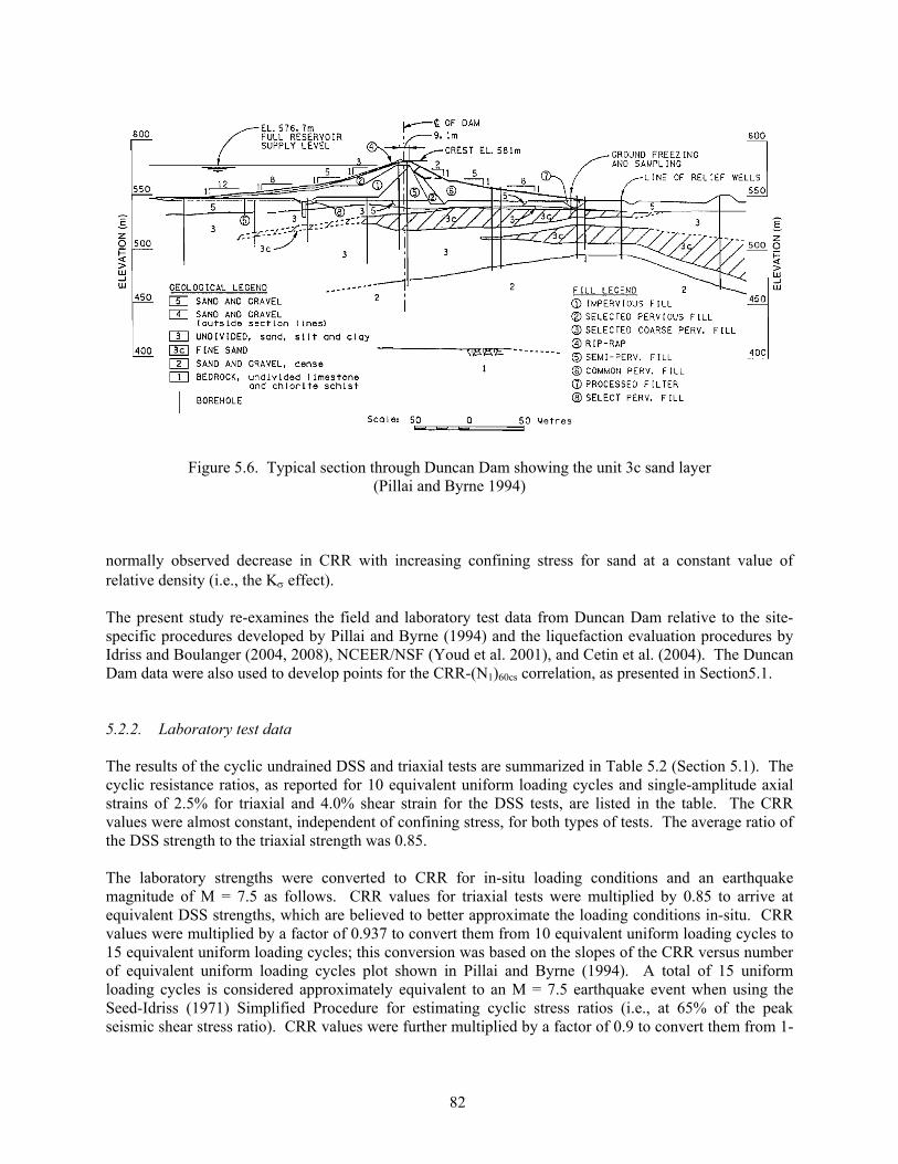
5.2. Duncan Dam – prediction of CRR at large overburden stresses 5.2.1. Background 5.2.2. Laboratory test data 5.2.3. Predicting the variation of CRR with depth based on SPT-based correlations 5.2.4. Values of CRR and (N1)60cs for Duncan Dam 5.2.5. Summary of comparisons 6. PROBABILISTIC RELATIONSHIP FOR LIQUEFACTION TRIGGERING 6.1. Probabilistic relationships for liquefaction triggering 6.2. Methodology 6.2.1. Limit state function 6.2.1. Likelihood function 6.3. Results of parameter estimation

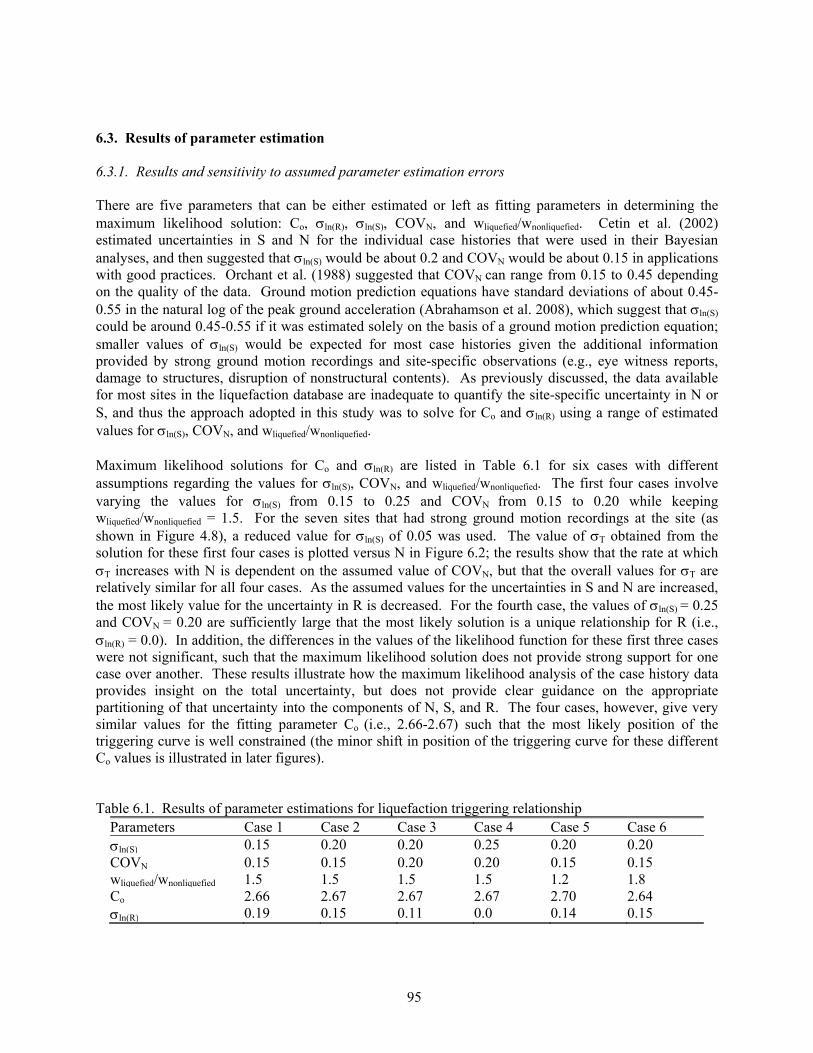
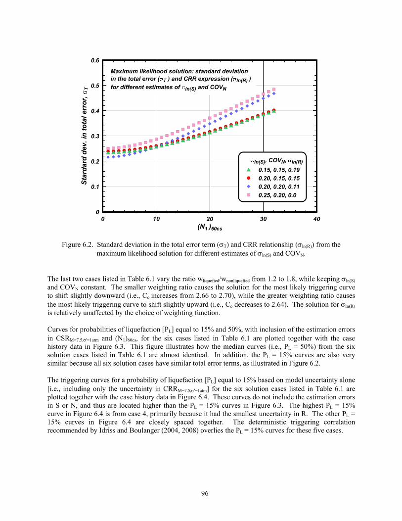
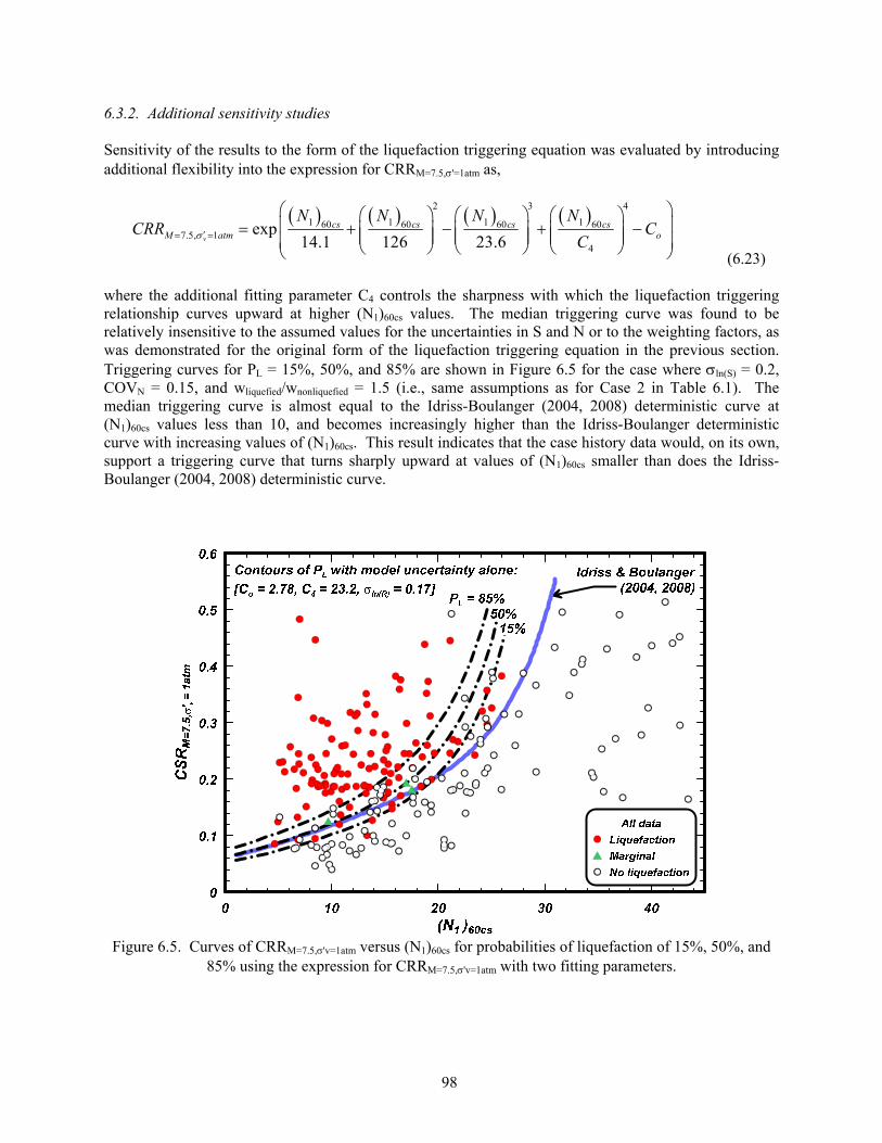
6.3.1. Results and sensitivity to assumed parameter estimation errors 6.3.2. Additional sensitivity studies 6.3.3. Recommended relationships

6.4. Summary

iii

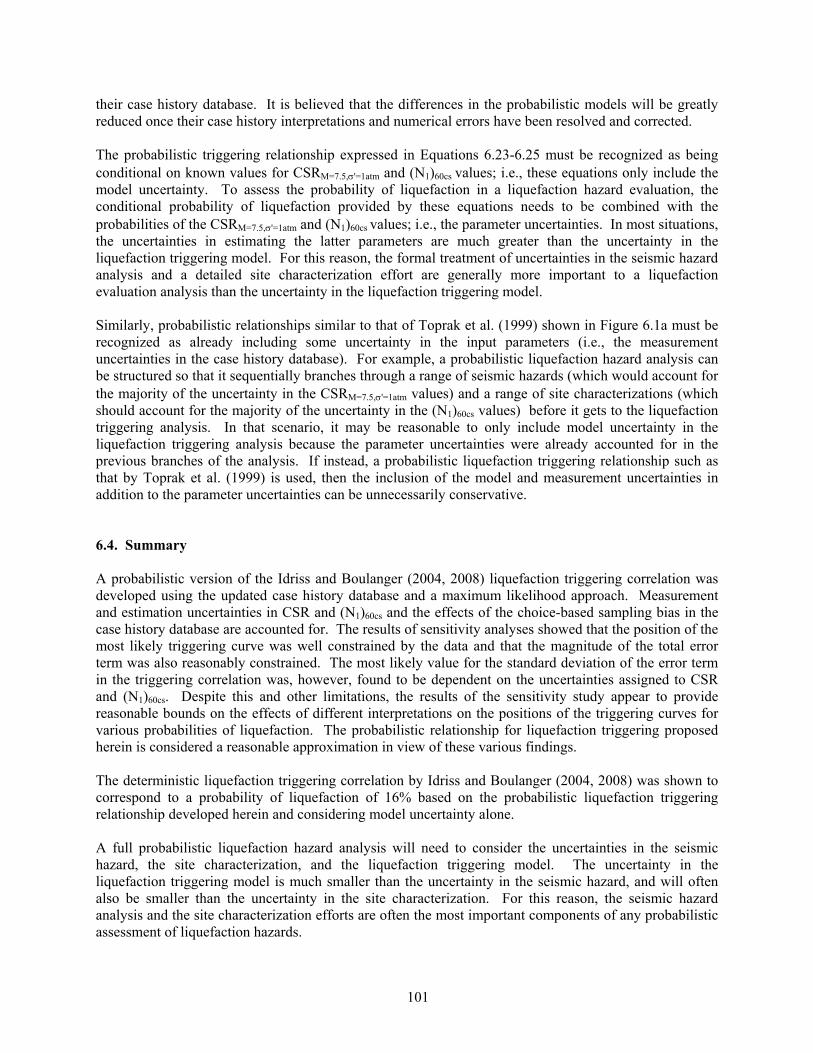
7. COMPARISON TO OTHER LIQUEFACTION TRIGGERING CORRELATIONS 7.1. Comparison of CRR values obtained using different triggering correlations 7.2. Reasons for the differences in the triggering correlations 7.3. Components affecting extrapolation outside the range of the case history data 7.3.1. Role of CN relationship 7.3.2. Role of K relationship 7.3.3. Role of rd relationship 7.3.4. Role of MSF relationship 8. SUMMARY AND CONCLUSIONS ACKNOWLEDGMENTS REFERENCES APPENDIX A: EXAMINATION OF THE CETIN ET AL. (2004) LIQUEFACTION TRIGGERING

CORRELATION APPENDIX B: SHEAR STRESS REDUCTION COEFFICIENT APPENDIX C: COMPUTATIONS OF REPRESENTATIVE (N1)60CS VALUES

1

SPT-based Liquefaction Triggering Procedures 1. INTRODUCTION 1.1. Purpose This report presents an updated examination of SPT-based liquefaction triggering procedures for cohesionless soils, with the specific purpose of: updating and documenting the case history database, providing more detailed illustrations of the database distributions relative to the liquefaction

triggering correlation by Idriss and Boulanger (2004, 2008), re-examining the database of cyclic test results for frozen sand samples, presenting a probabilistic version of the Idriss-Boulanger (2004, 2008) liquefaction triggering

correlation using the updated case history database, presenting a number of new findings regarding components of the liquefaction analysis framework

used to interpret and extend the case history experiences, and presenting an examination of the reasons for the differences between some current liquefaction

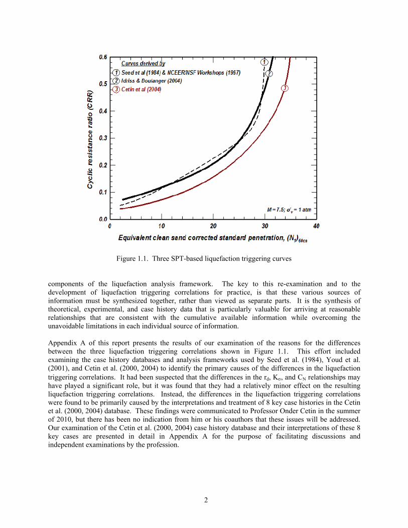
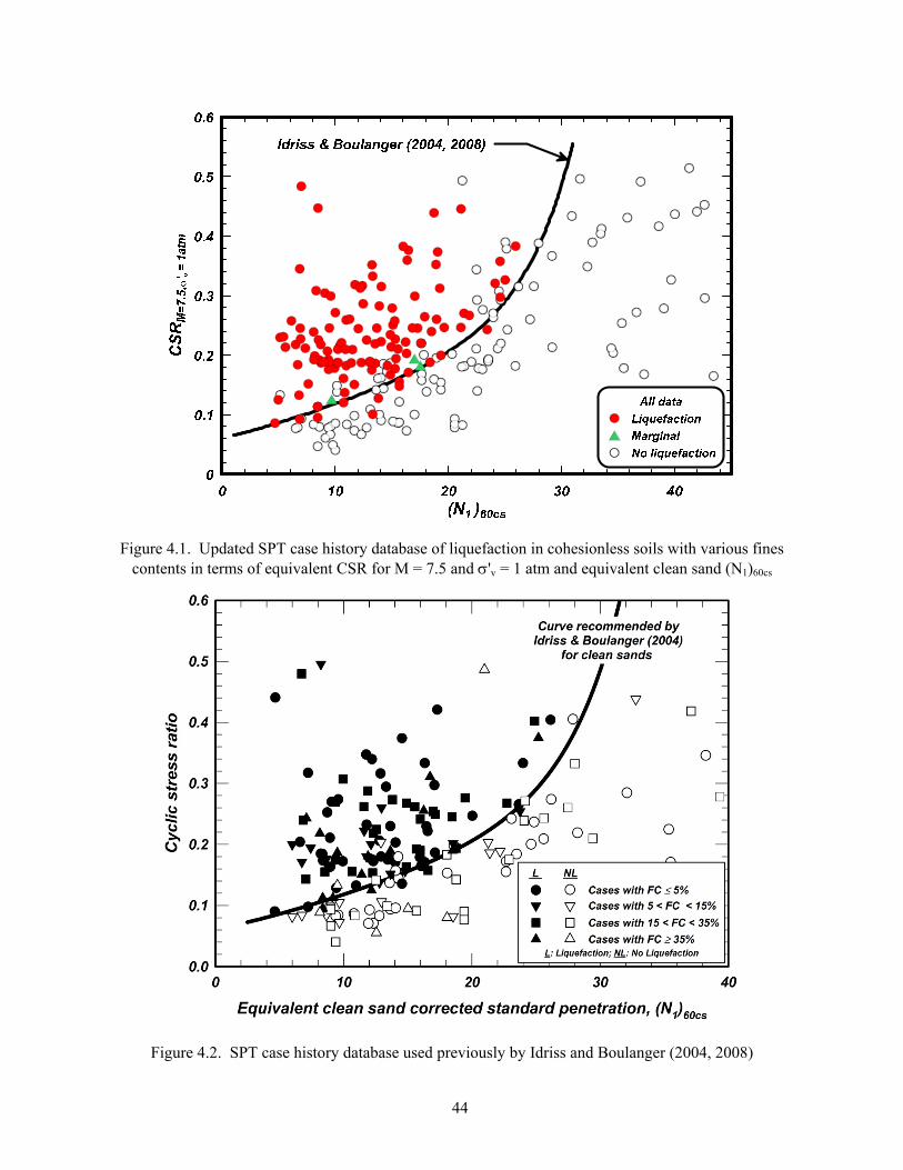
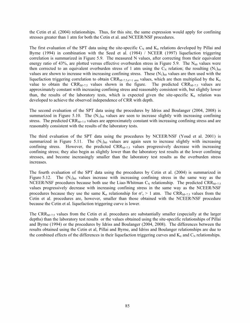
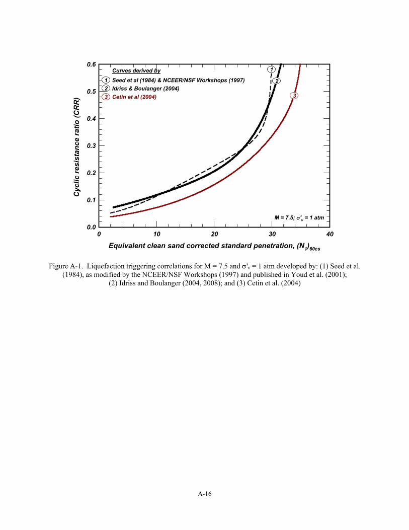
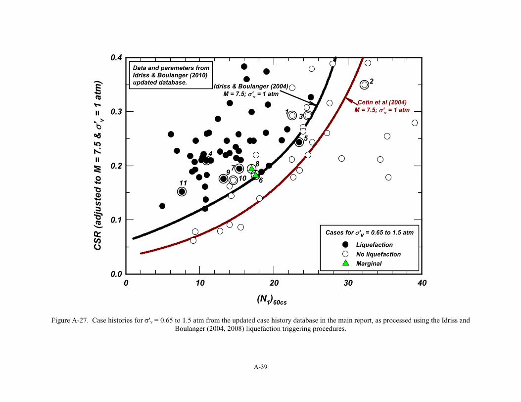
triggering correlations. The last task addresses an issue of current importance to the profession, which specifically pertains to determining the source of the differences between the liquefaction triggering correlations published by the late Professor H. Bolton Seed and colleagues (Seed et al. 1984, 1985), which were adopted with slight modifications in the NCEER/NSF workshops (Youd et al. 2001), and those published more recently by Cetin et al. (2004) and those published by Idriss and Boulanger (2004, 2008). These liquefaction triggering correlations are compared in Figure 1.1 in terms of the cyclic resistance ratio (CRR) adjusted for M = 7.5 and 'v = 1 atm versus (N1)60cs. The question of concern is why the correlation of CRRM=7.5,'=1 versus (N1)60cs proposed by Cetin et al. (2004) is significantly lower than those by Seed et al. (1984) and those by Idriss and Boulanger (2004, 2008) although they are based on largely the same case histories. Do these differences represent scientific (epistemic) uncertainty, or are they due to errors or biases in the analysis frameworks or case history interpretations that can be resolved? This issue became important to the profession in 2010 when Professor Raymond B. Seed stated that the use of the Idriss-Boulanger correlations, and presumably the similar Seed et al. (1984) correlation, was "dangerously unconservative." He repeated such statements in a series of visits to major consulting firms and regulatory agencies, a series of e-mail messages to the EERI Board of Directors with copies to over 100 prominent individuals in the USA and abroad, and a University of California at Berkeley Geotechnical Report titled, "Technical Review and Comments: 2008 EERI Monograph (by I.M. Idriss and R.W. Boulanger)". These statements took us by surprise, caused some degree of concern within the profession, and left many people asking: "Why the controversy" and "Why in this way?" We cannot answer these questions, but we can take this opportunity to openly and carefully re-examine the key technical issues affecting liquefaction triggering correlations and to investigate the reasons for the differences among the three correlations shown in Figure 1.1. The body of this report presents the results of this updated re-examination of SPT-based liquefaction triggering procedures. This re-examination included updating the case history database, re-examining how the case history data compare to the database of cyclic test results for frozen sand samples, re-examining the case history data in a probabilistic framework, and examining new findings regarding

2

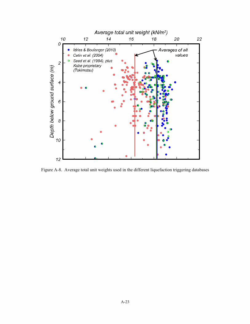
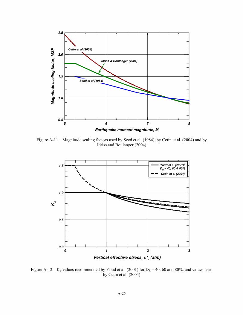
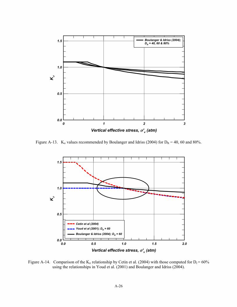
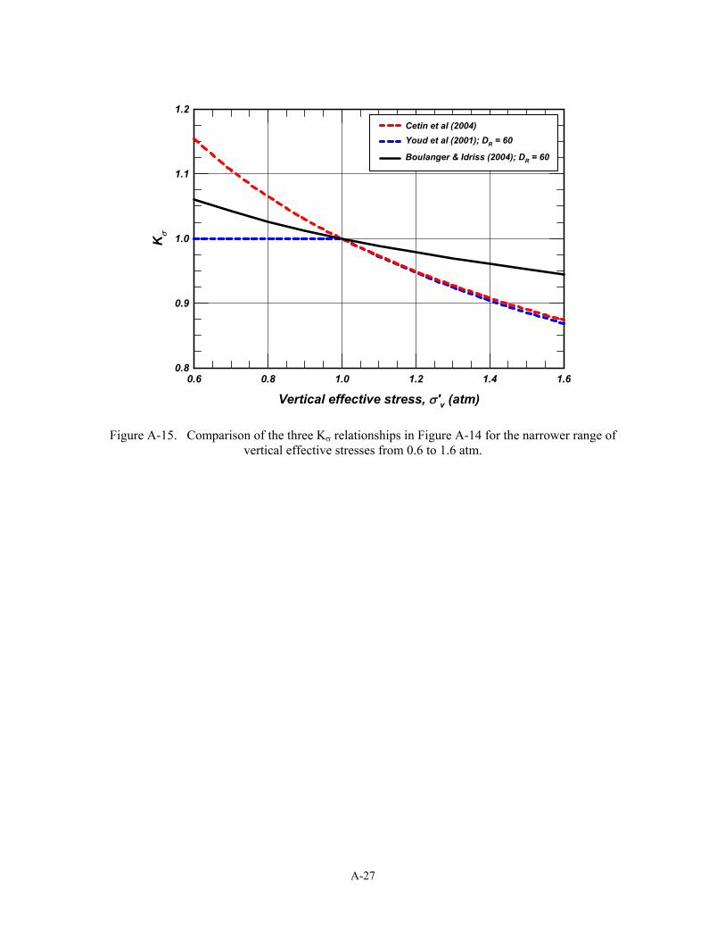
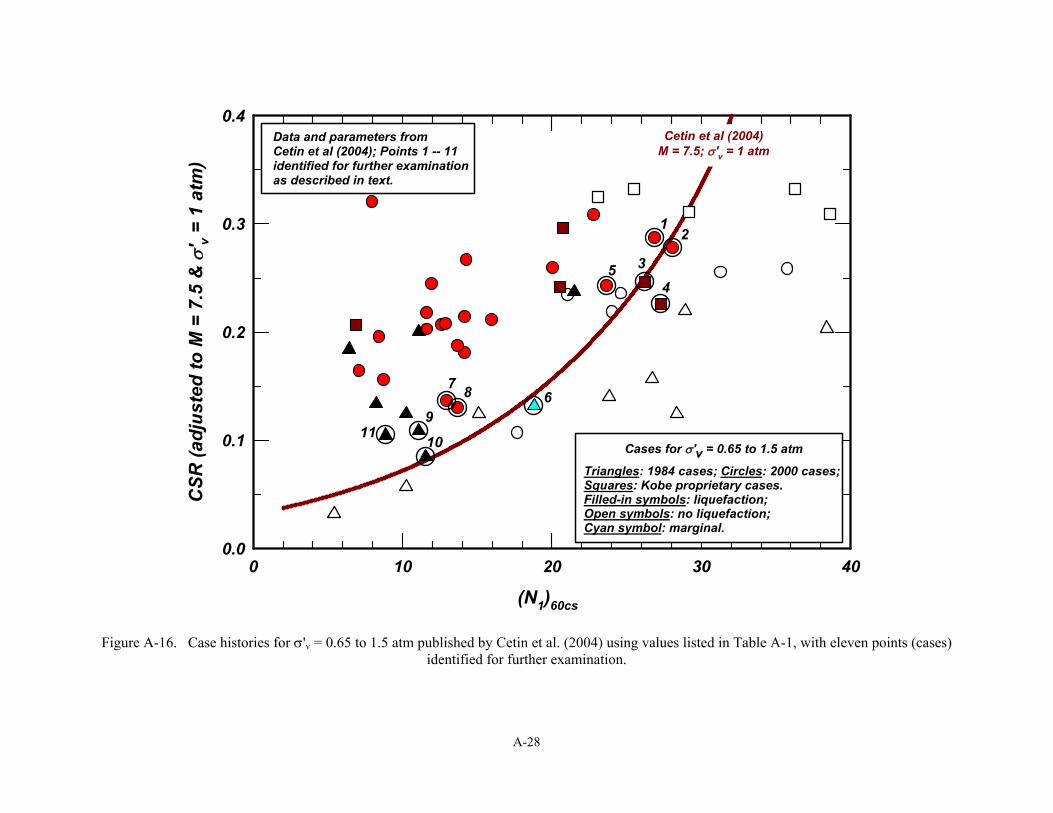
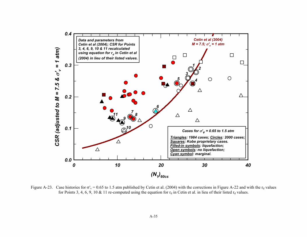
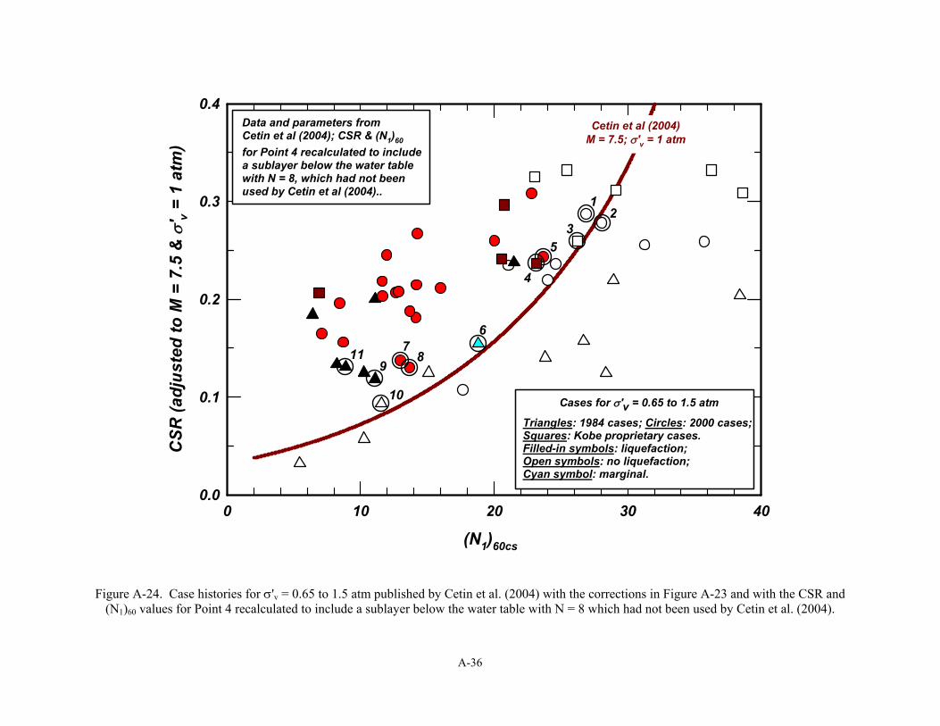
components of the liquefaction analysis framework. The key to this re-examination and to the development of liquefaction triggering correlations for practice, is that these various sources of information must be synthesized together, rather than viewed as separate parts. It is the synthesis of theoretical, experimental, and case history data that is particularly valuable for arriving at reasonable relationships that are consistent with the cumulative available information while overcoming the unavoidable limitations in each individual source of information. Appendix A of this report presents the results of our examination of the reasons for the differences between the three liquefaction triggering correlations shown in Figure 1.1. This effort included examining the case history databases and analysis frameworks used by Seed et al. (1984), Youd et al. (2001), and Cetin et al. (2000, 2004) to identify the primary causes of the differences in the liquefaction triggering correlations. It had been suspected that the differences in the rd, K, and CN relationships may have played a significant role, but it was found that they had a relatively minor effect on the resulting liquefaction triggering correlations. Instead, the differences in the liquefaction triggering correlations were found to be primarily caused by the interpretations and treatment of 8 key case histories in the Cetin et al. (2000, 2004) database. These findings were communicated to Professor Onder Cetin in the summer of 2010, but there has been no indication from him or his coauthors that these issues will be addressed. Our examination of the Cetin et al. (2000, 2004) case history database and their interpretations of these 8 key cases are presented in detail in Appendix A for the purpose of facilitating discussions and independent examinations by the profession.

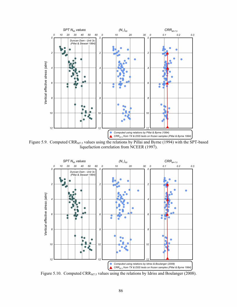
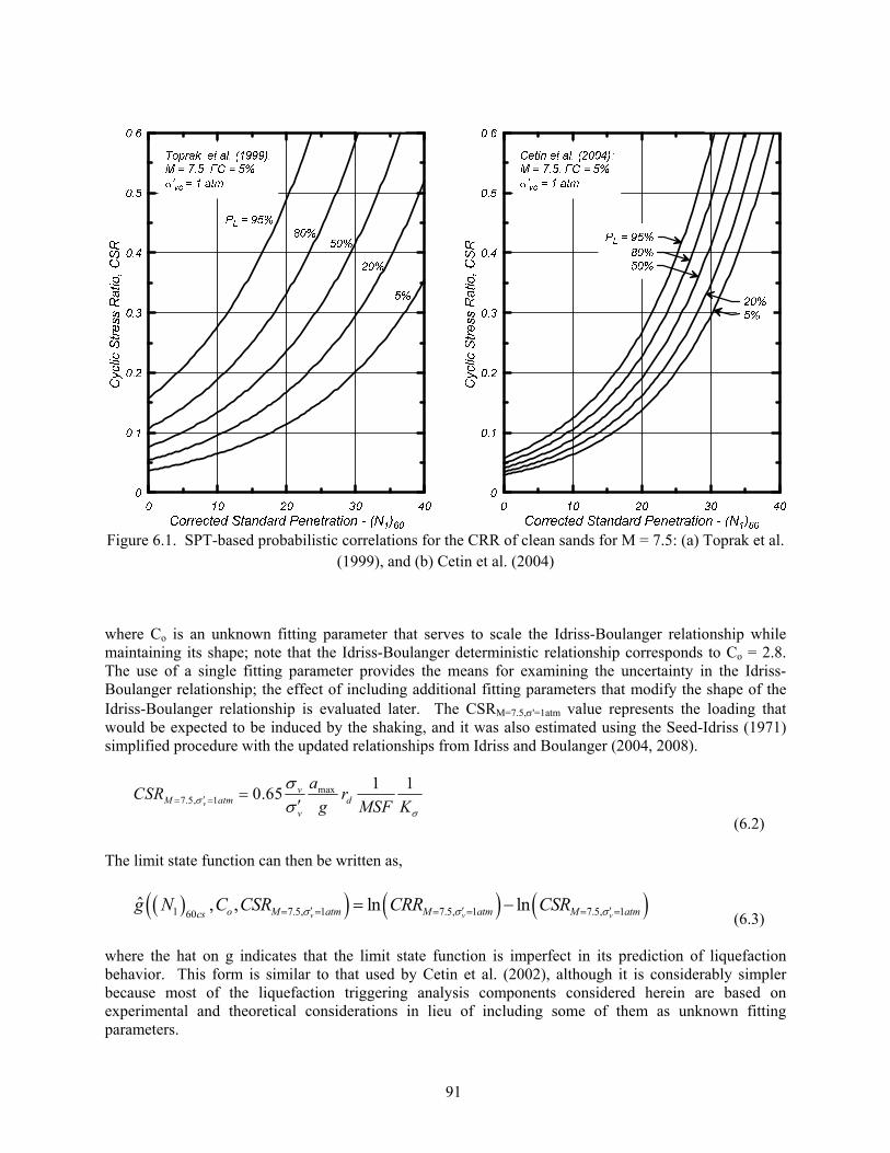
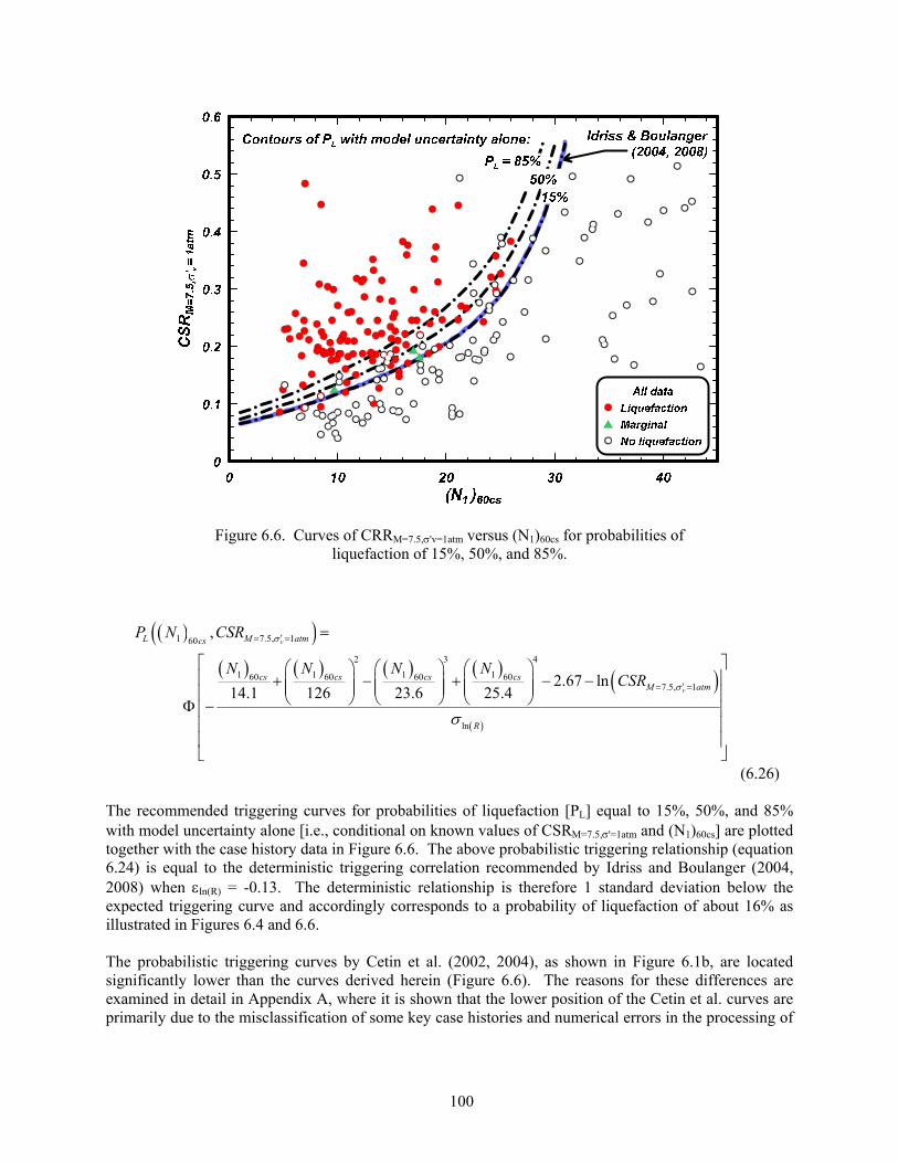
Figure 1.1. Three SPT-based liquefaction triggering curves

3

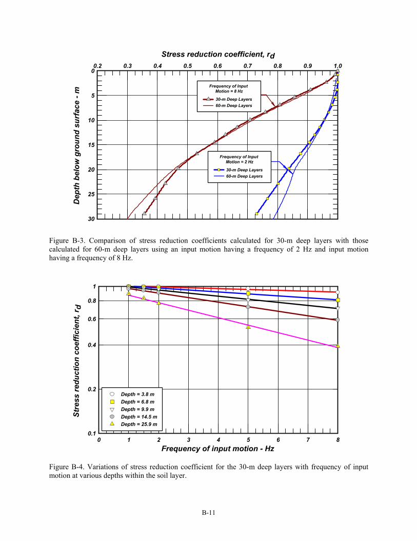
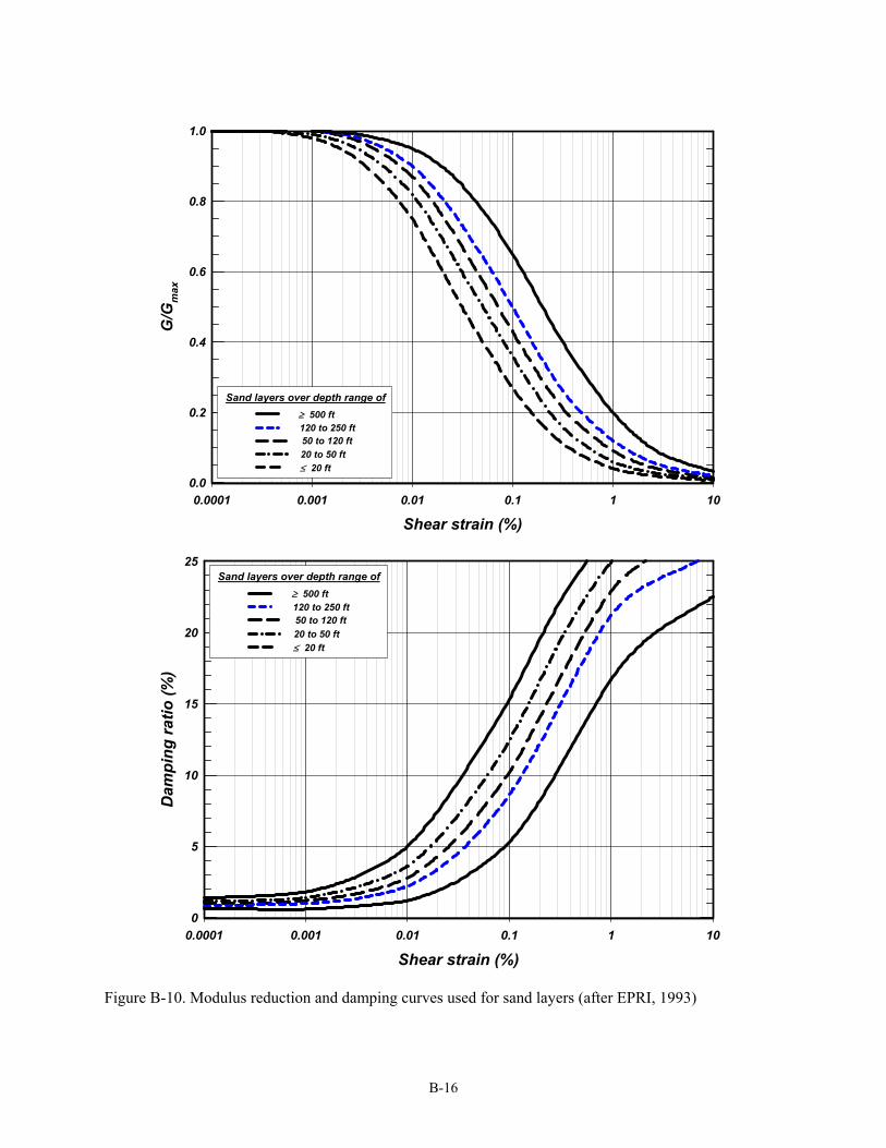
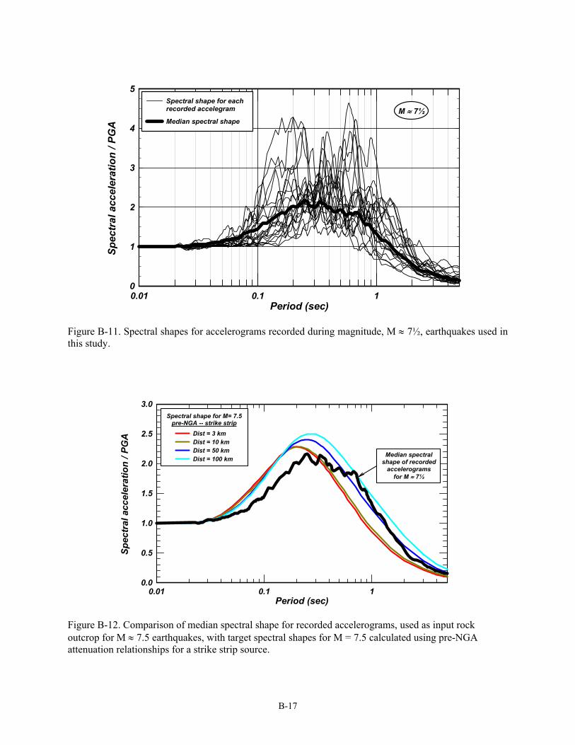
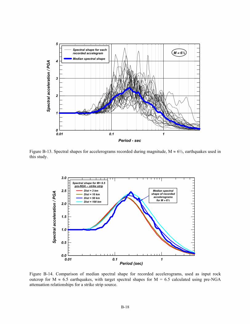
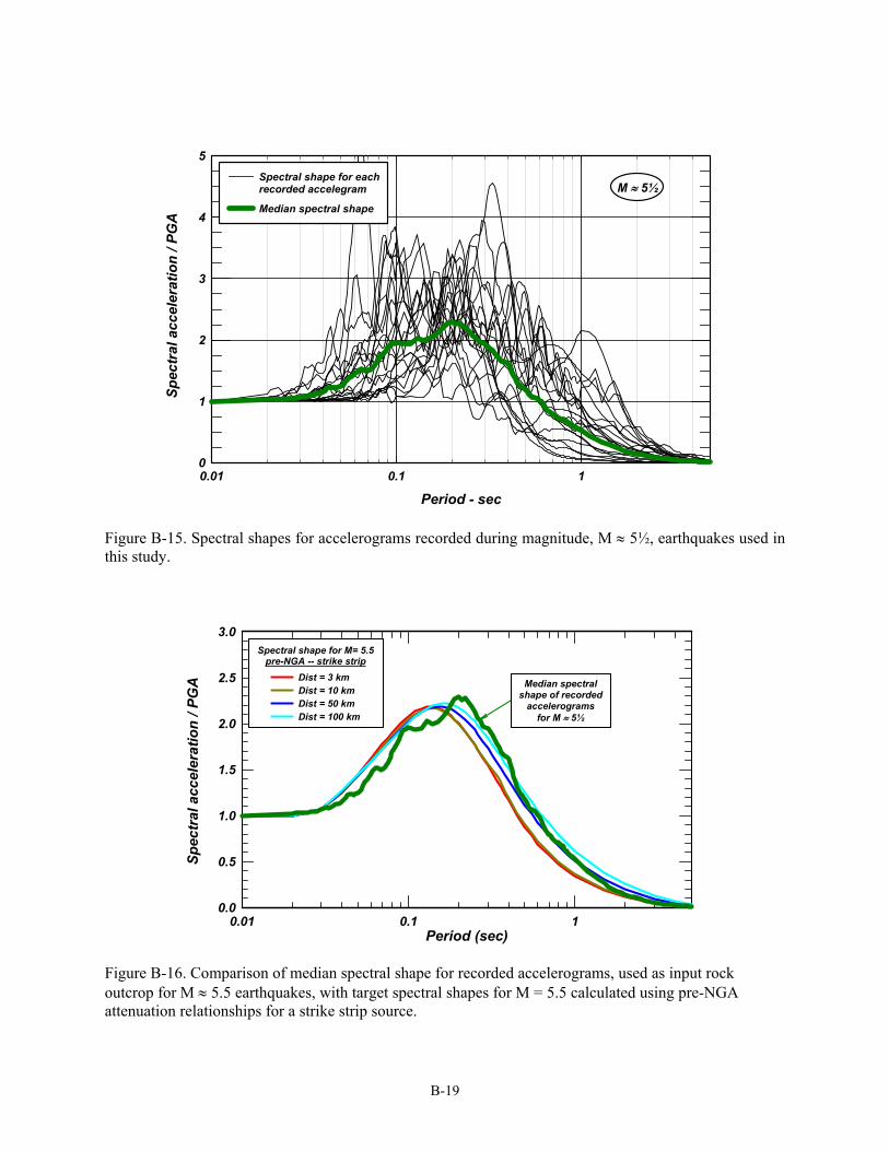
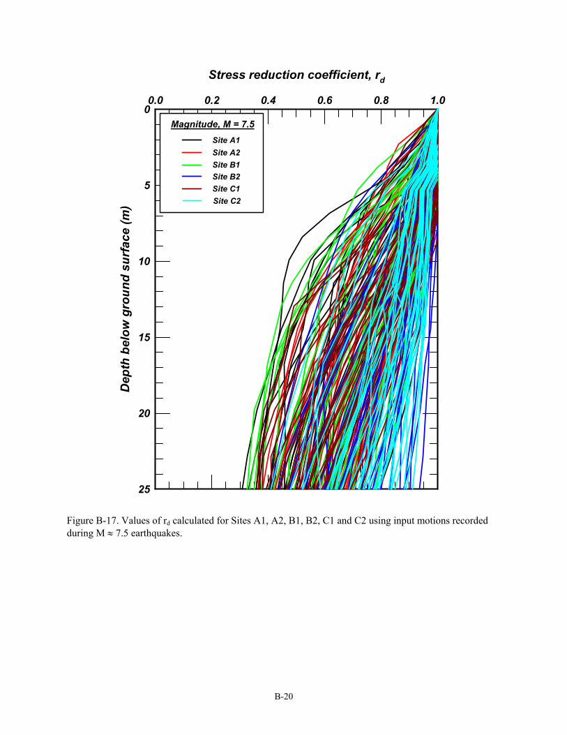
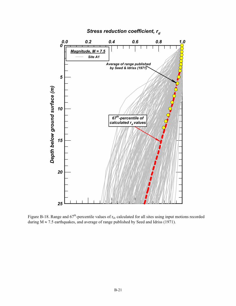
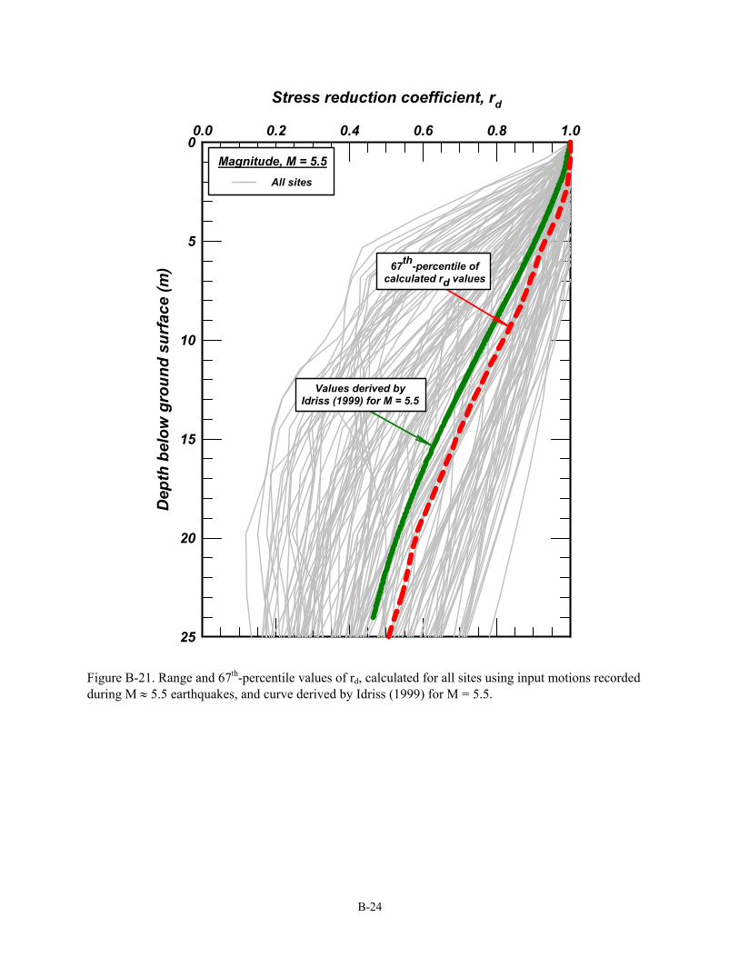
It is hoped that this report will serve as a useful resource for practicing engineers and researchers working in the field of soil liquefaction. It is also hoped that this report will be a useful technical supplement to the 2008 EERI Monograph on Soil Liquefaction During Earthquakes by Idriss and Boulanger (2008). 1.2. Organization of report Section 2 of this report contains an overview of the SPT-based liquefaction analysis framework for cohesionless soils, followed by a summary of the specific relationships used or derived by Idriss and Boulanger (2004, 2008). Section 3 describes the updated database of SPT-based liquefaction/no liquefaction case histories. The selection of earthquake magnitudes, peak accelerations, and representative (N1)60cs values are described, and the classification of site performance discussed. Section 4 provides an evaluation of the SPT-based liquefaction triggering database relative to the liquefaction triggering correlation by Idriss and Boulanger (2004, 2008). The distributions of the data are examined with respect to various parameters (e.g., fines content, overburden stress, earthquake magnitude) and data sources (e.g., data from the U.S., Japan, pre- and post-1985 studies, and sites with strong ground motion recordings). In addition, the sensitivity of the database's interpretation to a number of aspects and components of the analysis framework is examined. Section 5 contains an examination of liquefaction triggering correlations developed using the results of cyclic laboratory tests on specimens obtained using frozen sampling techniques (e.g., Yoshimi et al. 1989, 1994) and their comparison to those derived from the field case histories. This section also contains a detailed examination of the unique set of field and laboratory testing data at large overburden stresses at Duncan Dam (e.g., Pillai and Byrne 1994). Section 6 describes the development of a probabilistic version of the Idriss and Boulanger (2004, 2008) liquefaction triggering correlation using the updated case history database and a maximum likelihood method. Sensitivity of the derived probabilistic relationship to the key assumptions is examined, and issues affecting the application of probabilistic liquefaction triggering models in practice are discussed. Section 7 contains a comparison of CRR values computed using some of the current liquefaction triggering correlations, followed by (1) a summary of the reasons for the differences in the derived triggering correlations, and (2) an examination of new findings regarding analysis components that affect how these triggering correlations are extrapolated outside the range of the case history data. Appendix A presents an examination of the Cetin et al. (2004) liquefaction triggering database and our findings regarding the primary reasons for the differences between the three liquefaction triggering correlations shown in Figure 1.1. Appendix B presents background information on the development of the Idriss (1999) relationship for the shear stress reduction coefficient, rd. Appendix C presents the computations for the (N1)60cs values in the liquefaction triggering database presented in this report.

4

2. ANALYSIS FRAMEWORK 2.1. Components of the stress-based framework The stress-based approach for evaluating the potential for liquefaction triggering, initiated by Seed and Idriss (1967), has been used widely for the last 45 years (e.g., Seed and Idriss 1971, Shibata 1981, Tokimatsu and Yoshimi 1983, NRC 1985, Seed et al. 1985, Youd et al. 2001, Cetin et al. 2004, Idriss and Boulanger 2004). The basic framework, as adopted by numerous researchers, compares the earthquake-induced cyclic stress ratios (CSR) with the cyclic resistance ratios (CRR) of the soil. The components of this framework, as briefly summarized below, were developed to provide a rational treatment of the various factors that affect penetration resistance and cyclic resistance. Earthquake-induced cyclic stress ratio (CSR) The earthquake-induced CSR, at a given depth, z, within the soil profile, is usually expressed as a representative value (or equivalent uniform value) equal to 65% of the maximum cyclic shear stress ratio, i.e.:

max, 0.65

vMv

CSR

(2.1)

where max = maximum earthquake induced shear stress, 'v = vertical effective stress, and the subscripts on the CSR indicate that it is computed for a specific earthquake magnitude (moment magnitude, M) and in-situ 'v. The choice of the reference stress level (i.e., the factor 0.65) was selected by Seed and Idriss (1967) and has been in use since. Selecting a different reference stress level would alter the values of certain parameters and relationships but would have no net effect on the final outcome of the derived liquefaction evaluation procedure, as long as this same reference stress level is used throughout, including forward calculations. The value of max can be estimated from dynamic response analyses, but such analyses must include a sufficient number of input acceleration time series and adequate site characterization details to be reasonably robust. Alternatively, the maximum shear stress can be estimated using the equation, developed as part of the Seed-Idriss Simplified Liquefaction Procedure, which is expressed as,

max, 0.65

v

vM d

v

aCSR r

g (2.2)

where v = vertical total stress at depth z, amax/g = maximum horizontal acceleration (as a fraction of gravity) at the ground surface, and rd = shear stress reduction factor that accounts for the dynamic response of the soil profile. Cyclic resistance ratio (CRR) The soil's CRR is usually correlated to an in-situ parameter such as SPT blow count (number of blows per foot), CPT penetration resistance or shear wave velocity, Vs. SPT blow counts are affected by a number of procedural details (rod lengths, hammer energy, sampler details, borehole size) and by effective overburden stress. Thus, the correlation to CRR is based on corrected penetration resistance,

5

1 60 N E R B S mN C C C C C N (2.3)

where CN is an overburden correction factor, CE = ERm/60%, ERm is the measured value of the delivered energy as a percentage of the theoretical free-fall hammer energy, CR is a rod correction factor to account for energy ratios being smaller with shorter rod lengths, CB is a correction factor for nonstandard borehole diameters, CS is a correction factor for using split spoons with room for liners but with the liners absent, and Nm is the measured SPT blow count. The factors CB and CS are set equal to unity if standard procedures are followed. The soil's CRR is also affected by the duration of shaking (which is correlated to the earthquake magnitude scaling factor, MSF) and effective overburden stress (which is expressed through a K factor). The correlation for CRR is therefore developed for a reference M = 7.5 and 'v = 1 atm, and then adjusted to other values of M and 'v using the following expression:

, 7.5, 1v vM MCRR CRR MSF K (2.4)

The soil's CRR is further affected by the presence of sustained static shear stresses, such as may exist beneath foundations or within slopes. This effect, which is expressed through a K factor, is generally small for nearly level ground conditions. It is not included herein because the case history database is dominated by level or nearly level ground conditions. The correlation of CRR to (N1)60 is affected by the soil's fines content (FC) and is expressed as,

7.5, 1 1 60,

vMCRR f N FC (2.5)

For mathematical convenience, this correlation can also be expressed in terms of an equivalent clean-sand (N1)60cs, which is obtained using the following expression:

1 1 160 60 60csN N N

(2.6)

CRR can then be expressed in terms of (N1)60cs, i.e.:

7.5, 1 1 60vcM csCRR f N

(2.7)

where the adjustment (N1)60 is a function of FC. The above framework has been used for a number of SPT-based liquefaction correlations, although the notation may be slightly different in some cases.

6

Important attributes of a liquefaction analysis procedure A liquefaction analysis procedure within the above stress-based framework requires the following two attributes: The liquefaction analysis procedure is applicable to the full range of conditions important to practice;

e.g., from shallow lateral spreads to large earth dams. Practice often results in the need to extrapolate outside the range of the case history experiences, requiring the framework to be supported by sound experimental and theoretical bases for guiding such extrapolations.

The mechanics are consistent with those used in developing companion correlations to other in-situ

parameters; e.g., SPT blow count, CPT penetration resistance, and shear wave velocity, Vs. Consistency in the mechanics facilitates the logical integration of information from multiple sources and provides a rational basis for the calibration of constitutive models for use in nonlinear dynamic analyses.

The components of the stress-based analysis framework include five functions, or relationships, that describe fundamental aspects of dynamic site response, penetration resistance, and soil characteristics and behavior. These five functions, along with the major factors affecting each, are:

rd = f(depth; earthquake and ground motion characteristics; dynamic soil properties) CN = f('v; DR; FC) CR = f(depth; rod stick-up length) K= f('v; DR; FC) MSF = f(earthquake and ground motion characteristics; soil characteristics)

These functions are best developed using a synthesis of empirical, experimental and theoretical methods, as ultimately the robustness of these functions is important for guiding the application of the resulting correlations to conditions that are not well-represented in the case history database. Statistical analyses and regression methods are valuable tools for examining liquefaction analysis methods and testing different hypotheses, but the functional relationships in the statistical models must be constrained and guided by available experimental data and theoretical considerations. In the case of liquefaction triggering correlations, the use of regression models alone to derive physical relationships is not considered adequate because: (1) the case history data are generally not sufficient to constrain the development of such relationships, as illustrated later in this report; (2) any such relationship will be dependent on the assumed forms for the other functions, particularly given that four of the above five functions are strongly dependent on depth; and (3) the use of regression to define functions describing fundamental behaviors does not necessarily produce a function that can be reliably used in extrapolating the resulting correlation to conditions not well represented in the database, such as large depths. These considerations are important to the examination of the reasons for differences among some current liquefaction analysis procedures, as discussed in Section 7 of this report. 2.2. Summary of the Idriss-Boulanger procedure The components of the analysis procedure used or derived by Idriss and Boulanger (2004, 2006, 2008) as part of their liquefaction triggering correlation are briefly summarized in this subsection.

7

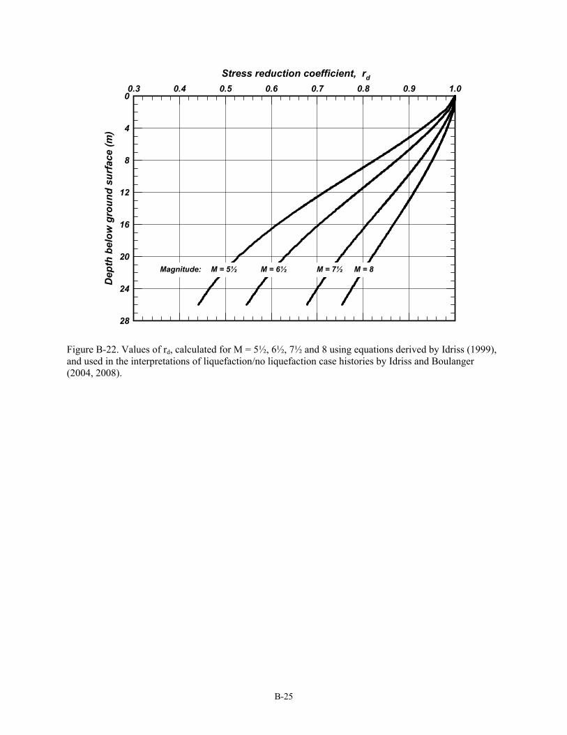
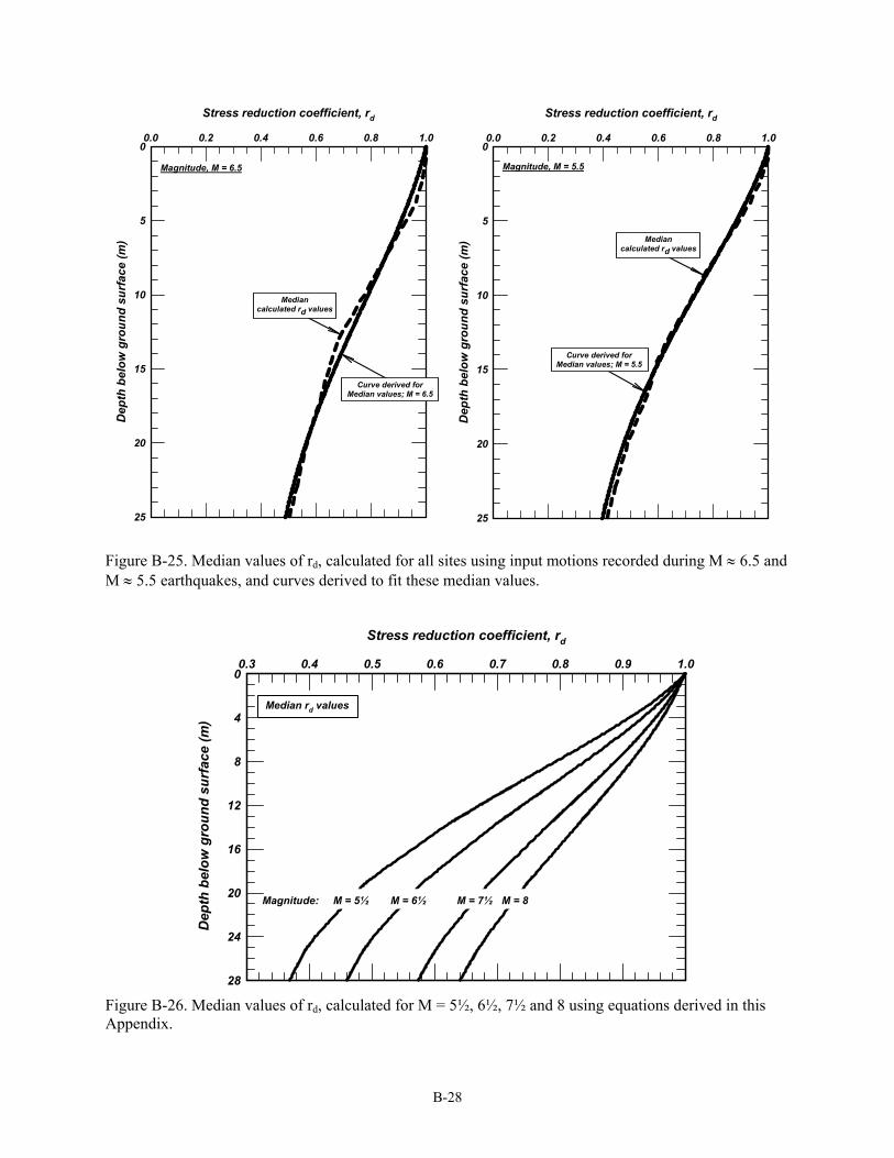
Shear stress reduction parameter, rd Idriss (1999), in extending the work of Golesorkhi (1989), performed several hundred parametric site response analyses and concluded that, for the purpose of developing liquefaction evaluation procedures, the parameter rd could be expressed as,

exp ( ) ( )

( ) 1.012 1.126sin 5.13311.73

( ) 0.106 0.118sin 5.14211.28

dr z z M

zz

zz

(2.8)

where z = depth below the ground surface in meters. The resulting relationship is plotted in Figure 2.1. Additional information on the development of this relationship is provided in Appendix C. Other rd relationships have been proposed, including the probabilistic relationships by Cetin et al. (2004) and Kishida et al. (2009b). The latter two relationships were based on large numbers of site response analyses for different site conditions and ground motions, and include the effects of a site's average shear wave velocity and the level of shaking. These alternative rd relationships and their effects on the interpretation of the liquefaction case histories are examined in Sections 4 and 6 of this report. Overburden correction factor, CN The CN relationship used was initially developed by Boulanger (2003) based on: (1) a re-examination of published SPT calibration chamber test data covering 'v of 0.7 to 5.4 atm (Marcuson and Bieganousky 1977a, 1977b); and (2) results of analyses for 'v of 0.2 to 20 atm using the cone penetration theory of Salgado et al. (1997a, 1997b) which was shown to produce good agreement with a database of over 400

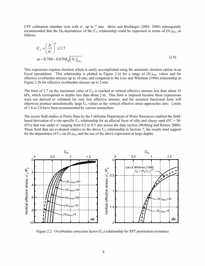
Figure 2.1. Shear stress reduction factor, rd, relationship

8

CPT calibration chamber tests with 'v up to 7 atm. Idriss and Boulanger (2003, 2008) subsequently recommended that the DR-dependence of the CN relationship could be expressed in terms of (N1)60cs as follows:

1 60

1.7

0.784 0.0768

m

aN

v

cs

PC

m N

(2.9)

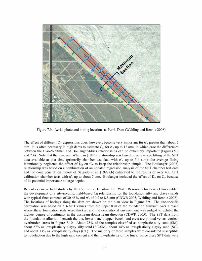
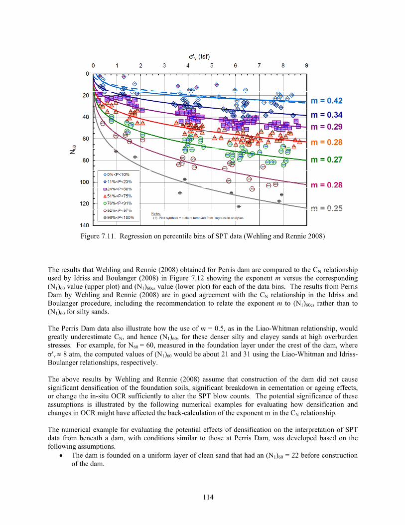
This expression requires iteration which is easily accomplished using the automatic iteration option in an Excel spreadsheet. This relationship is plotted in Figure 2.2a for a range of (N1)60cs values and for effective overburden stresses up to 10 atm, and compared to the Liao and Whitman (1986) relationship in Figure 2.2b for effective overburden stresses up to 2 atm. The limit of 1.7 on the maximum value of CN is reached at vertical effective stresses less than about 35 kPa, which corresponds to depths less than about 2 m. This limit is imposed because these expressions were not derived or validated for very low effective stresses, and the assumed functional form will otherwise produce unrealistically large CN values as the vertical effective stress approaches zero. Limits of 1.6 to 2.0 have been recommended by various researchers. The recent field studies at Perris Dam by the California Department of Water Resources enabled the field-based derivation of a site-specific CN relationship for an alluvial layer of silty and clayey sand (FC = 30-45%) that was under 'v ranging from 0.2 to 8.5 atm across the dam section (Wehling and Rennie 2008). These field data are evaluated relative to the above CN relationship in Section 7; the results lend support for the dependence of CN on (N1)60cs

and the use of the above expression at large depths.

Figure 2.2. Overburden correction factor (CN) relationship for SPT penetration resistance

0 0.5 1 1.5

CN

10

8

6

4

2

0

Ve

rtic

alef

fect

ive

stre

ss,

' v/P

a

(N1)60cs=40

(N1)60cs=30

(N1)60cs=20

(N1)60cs=10

(N1)60cs=4

0 0.5 1 1.5

CN

2

1.5

1

0.5

0

Ver

tica

leffe

ctiv

est

ress

, ' v

/Pa

(a) (b)

(N1)60cs=4

(N1)60cs=30

Liao & Whitman (1986)CN = (Pa /'v )0.5

9

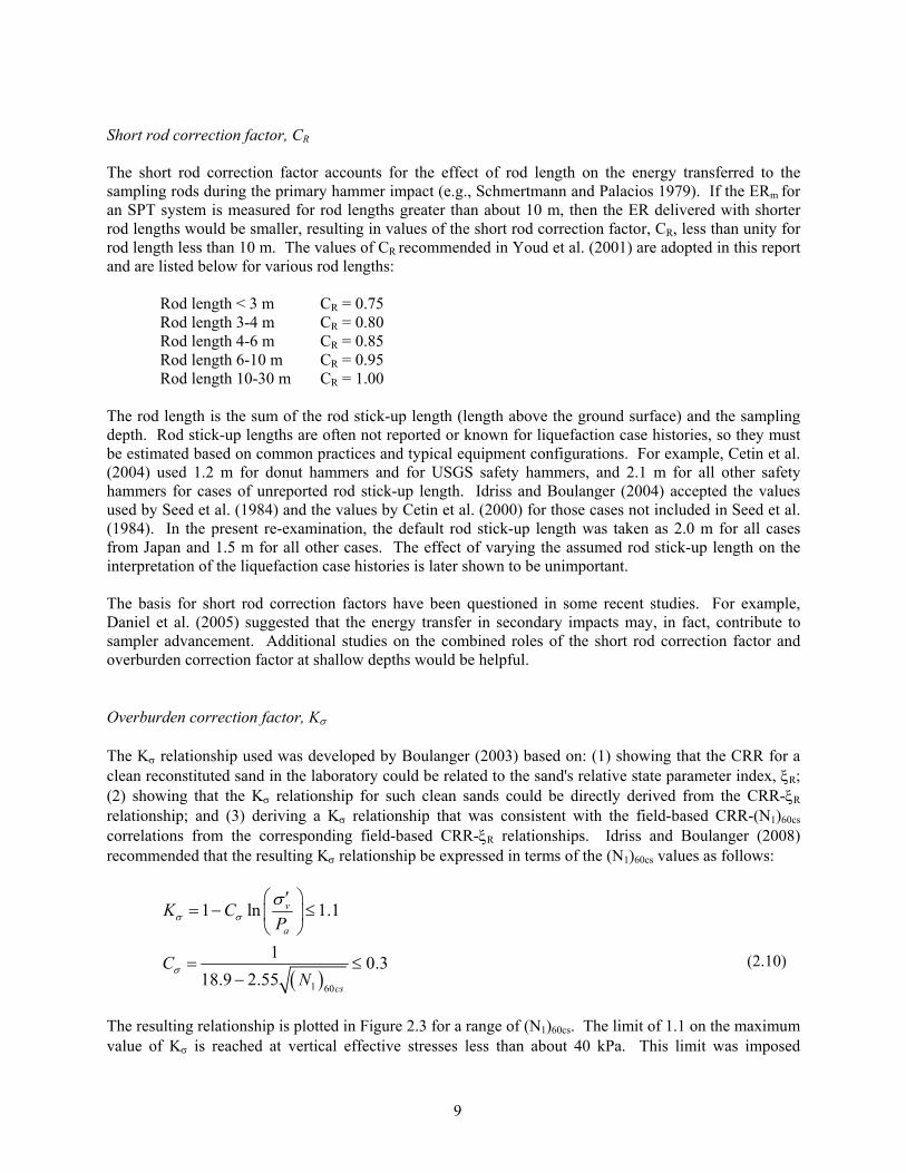
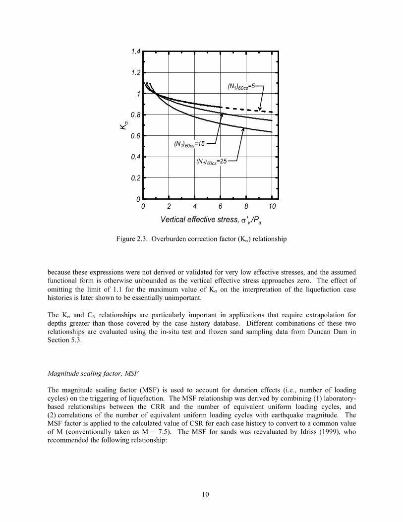
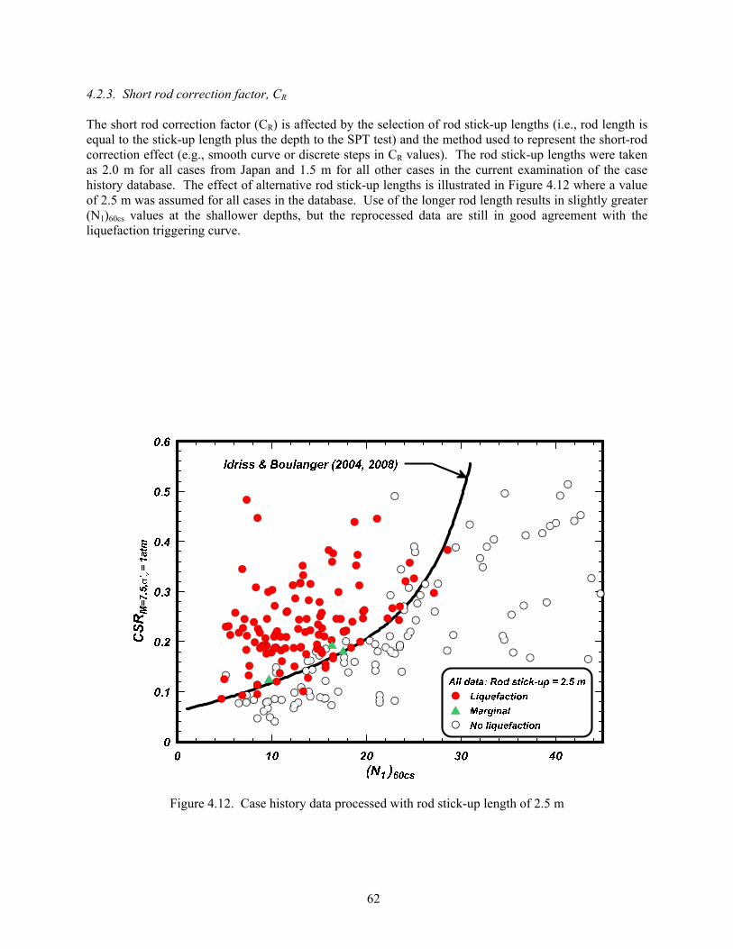
Short rod correction factor, CR The short rod correction factor accounts for the effect of rod length on the energy transferred to the sampling rods during the primary hammer impact (e.g., Schmertmann and Palacios 1979). If the ERm for an SPT system is measured for rod lengths greater than about 10 m, then the ER delivered with shorter rod lengths would be smaller, resulting in values of the short rod correction factor, CR, less than unity for rod length less than 10 m. The values of CR recommended in Youd et al. (2001) are adopted in this report and are listed below for various rod lengths: Rod length < 3 m CR = 0.75 Rod length 3-4 m CR = 0.80 Rod length 4-6 m CR = 0.85 Rod length 6-10 m CR = 0.95 Rod length 10-30 m CR = 1.00 The rod length is the sum of the rod stick-up length (length above the ground surface) and the sampling depth. Rod stick-up lengths are often not reported or known for liquefaction case histories, so they must be estimated based on common practices and typical equipment configurations. For example, Cetin et al. (2004) used 1.2 m for donut hammers and for USGS safety hammers, and 2.1 m for all other safety hammers for cases of unreported rod stick-up length. Idriss and Boulanger (2004) accepted the values used by Seed et al. (1984) and the values by Cetin et al. (2000) for those cases not included in Seed et al. (1984). In the present re-examination, the default rod stick-up length was taken as 2.0 m for all cases from Japan and 1.5 m for all other cases. The effect of varying the assumed rod stick-up length on the interpretation of the liquefaction case histories is later shown to be unimportant. The basis for short rod correction factors have been questioned in some recent studies. For example, Daniel et al. (2005) suggested that the energy transfer in secondary impacts may, in fact, contribute to sampler advancement. Additional studies on the combined roles of the short rod correction factor and overburden correction factor at shallow depths would be helpful. Overburden correction factor, K The K relationship used was developed by Boulanger (2003) based on: (1) showing that the CRR for a clean reconstituted sand in the laboratory could be related to the sand's relative state parameter index, R; (2) showing that the K relationship for such clean sands could be directly derived from the CRR-R relationship; and (3) deriving a K relationship that was consistent with the field-based CRR-(N1)60cs correlations from the corresponding field-based CRR-R relationships. Idriss and Boulanger (2008) recommended that the resulting K relationship be expressed in terms of the (N1)60cs values as follows:

1 60

1 ln 1.1

10.3

18.9 2.55

v

a

cs

K CP

CN

(2.10)

The resulting relationship is plotted in Figure 2.3 for a range of (N1)60cs. The limit of 1.1 on the maximum value of K is reached at vertical effective stresses less than about 40 kPa. This limit was imposed

10

because these expressions were not derived or validated for very low effective stresses, and the assumed functional form is otherwise unbounded as the vertical effective stress approaches zero. The effect of omitting the limit of 1.1 for the maximum value of K on the interpretation of the liquefaction case histories is later shown to be essentially unimportant. The K and CN relationships are particularly important in applications that require extrapolation for depths greater than those covered by the case history database. Different combinations of these two relationships are evaluated using the in-situ test and frozen sand sampling data from Duncan Dam in Section 5.3. Magnitude scaling factor, MSF The magnitude scaling factor (MSF) is used to account for duration effects (i.e., number of loading cycles) on the triggering of liquefaction. The MSF relationship was derived by combining (1) laboratory-based relationships between the CRR and the number of equivalent uniform loading cycles, and (2) correlations of the number of equivalent uniform loading cycles with earthquake magnitude. The MSF factor is applied to the calculated value of CSR for each case history to convert to a common value of M (conventionally taken as M = 7.5). The MSF for sands was reevaluated by Idriss (1999), who recommended the following relationship:

Figure 2.3. Overburden correction factor (K) relationship

0 2 4 6 8 10

Vertical effective stress, 'v /Pa

0

0.2

0.4

0.6

0.8

1

1.2

1.4

K

(N1)60cs=25

(N1)60cs=15

(N1)60cs=5

11

6.9 exp 0.058 1.84

MMSF

(2.11)

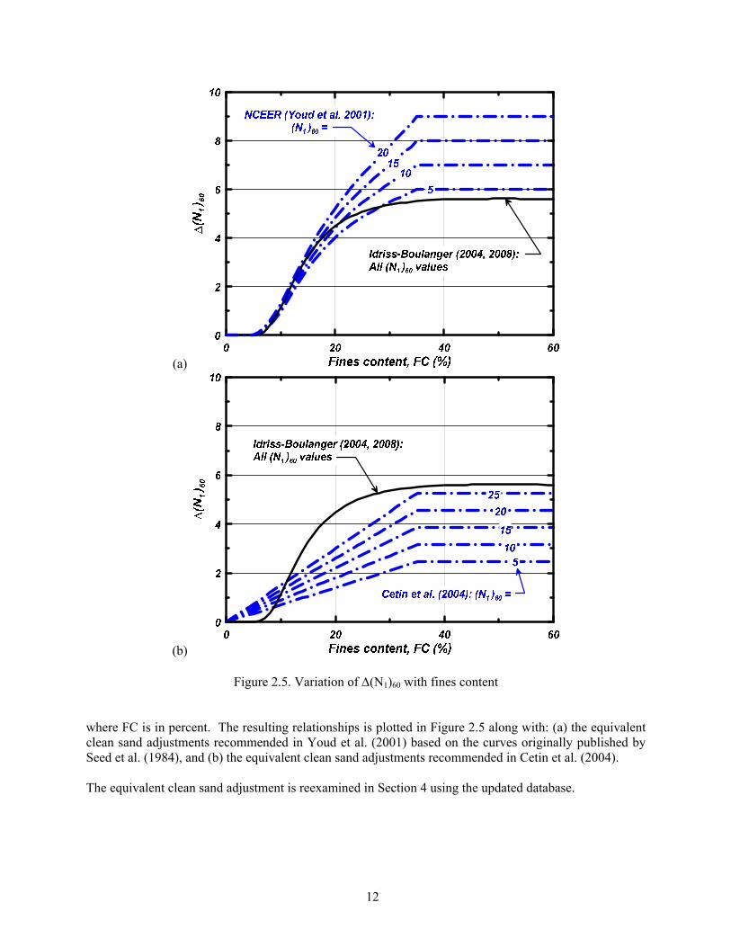
An upper limit for the MSF is assigned to very-small-magnitude earthquakes for which a single peak stress can dominate the entire time series. The value of 1.8 is obtained by considering the time series of stress induced by a small magnitude earthquake to be dominated by single pulse of stress (i.e., ½ to 1 full cycle, depending on its symmetry), with all other stress cycles being sufficiently small to neglect. The resulting relationship is plotted in Figure 2.4. Equivalent clean sand adjustment, (N1)60 The equivalent clean sand adjustment, (N1)60, is empirically derived from the liquefaction case history data, and accounts for the effects that fines content has on both the CRR and the SPT blow count. The liquefaction case histories suggest that the liquefaction triggering correlation shifts to the left as the fines content (FC) increases. This effect is conveniently represented by adjusting the SPT (N1)60 values to equivalent clean sand (N1)60cs values (equation 2.6), and then expressing CRR as a function of (N1)60cs. The equivalent clean sand adjustment developed by Idriss and Boulanger (2004, 2008) is expressed as,

2

1 60

9.7 15.7exp 1.63

0.01 0.01N

FC FC

(2.12)

Figure 2.4. Magnitude scaling factor (MSF) relationship

Earthquake moment magnitude, M

5 6 7 8 9

Mag

nit

ud

e sc

alin

g f

acto

r, M

SF

0

1

2

3

Seed & Idriss (1982)

Ambraseys (1985)

Arango (1996)

Idriss (1999)

Tokimatsu & Yoshimi (1983)

Cetin et al (2004)

MMSF 6.9exp 0.058

4

12

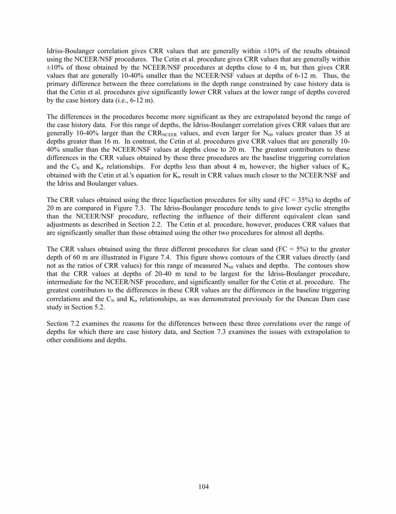
where FC is in percent. The resulting relationships is plotted in Figure 2.5 along with: (a) the equivalent clean sand adjustments recommended in Youd et al. (2001) based on the curves originally published by Seed et al. (1984), and (b) the equivalent clean sand adjustments recommended in Cetin et al. (2004). The equivalent clean sand adjustment is reexamined in Section 4 using the updated database.

(a)

(b)

Figure 2.5. Variation of (N1)60 with fines content

13

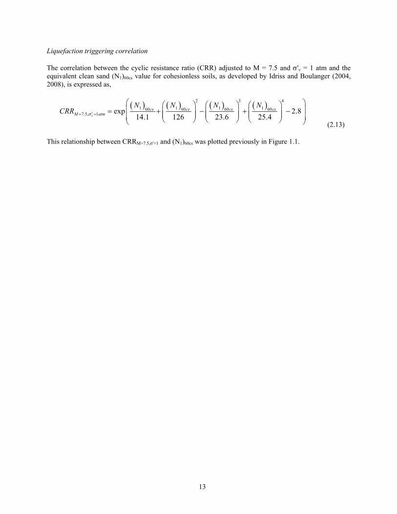
Liquefaction triggering correlation The correlation between the cyclic resistance ratio (CRR) adjusted to M = 7.5 and 'v = 1 atm and the equivalent clean sand (N1)60cs value for cohesionless soils, as developed by Idriss and Boulanger (2004, 2008), is expressed as,

2 3 4

1 1 1 160 60 60 607.5, 1 exp 2.8

14.1 126 23.6 25.4v

cs cs cs csM atm

N N N NCRR

(2.13)

This relationship between CRRM=7.5,'=1 and (N1)60cs was plotted previously in Figure 1.1.

14

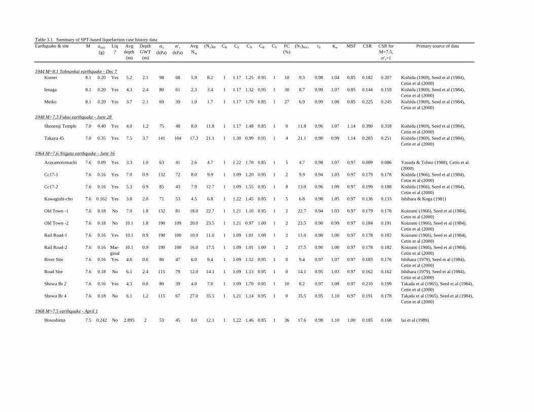
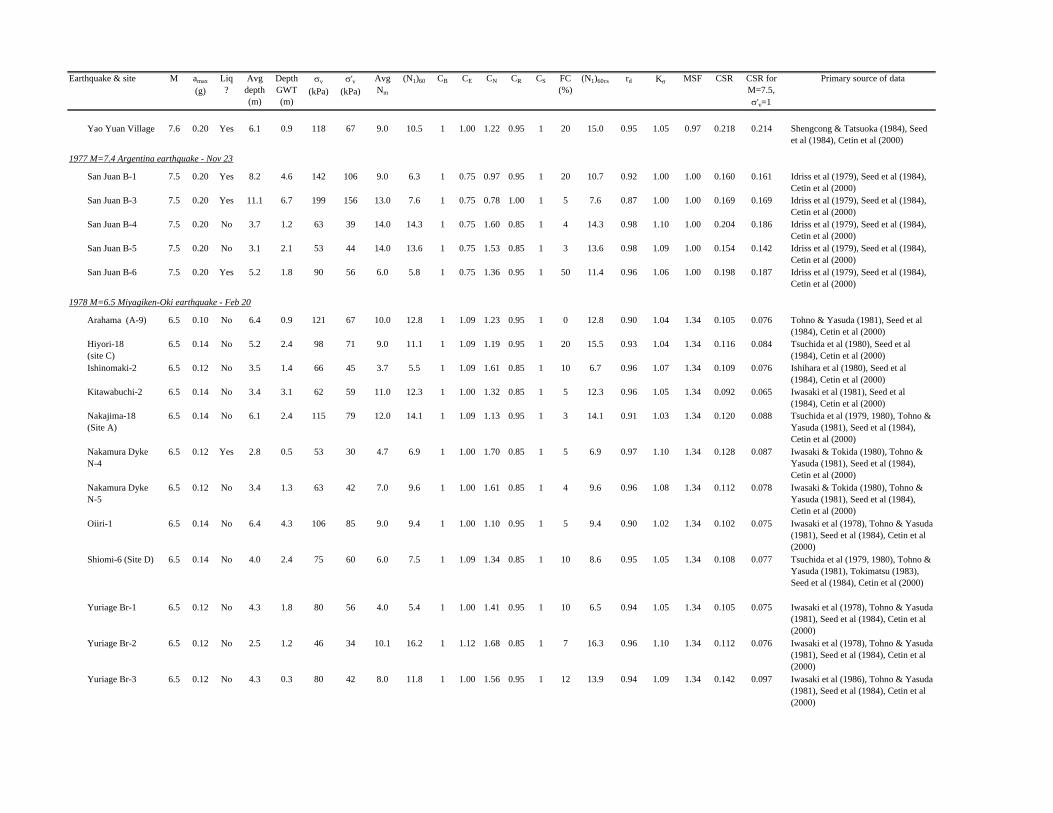
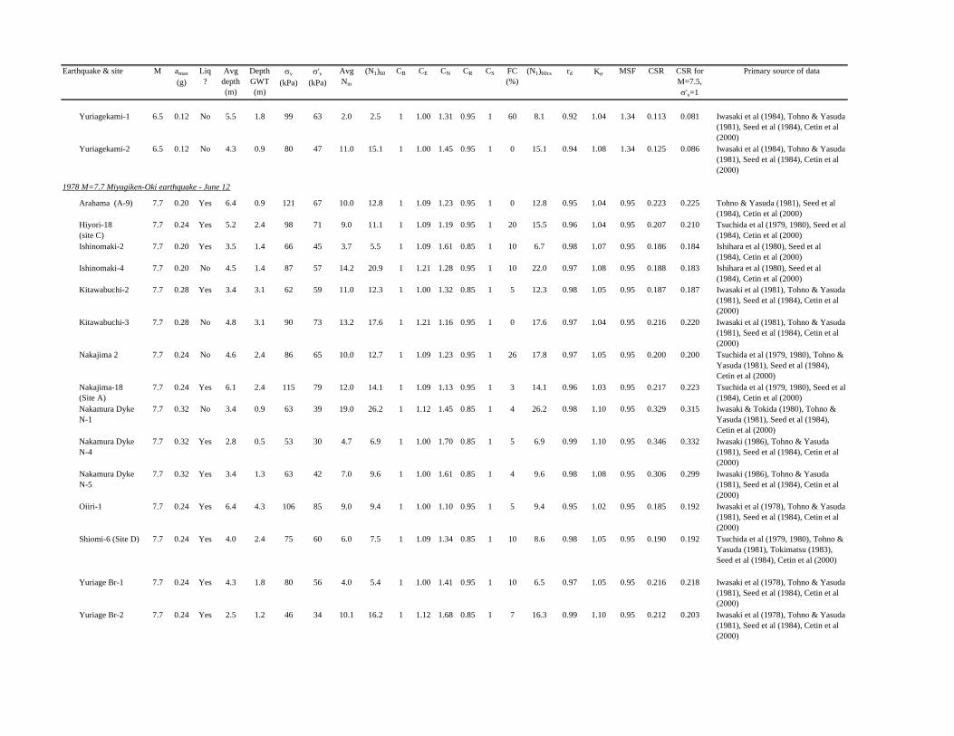
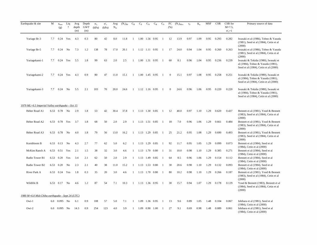
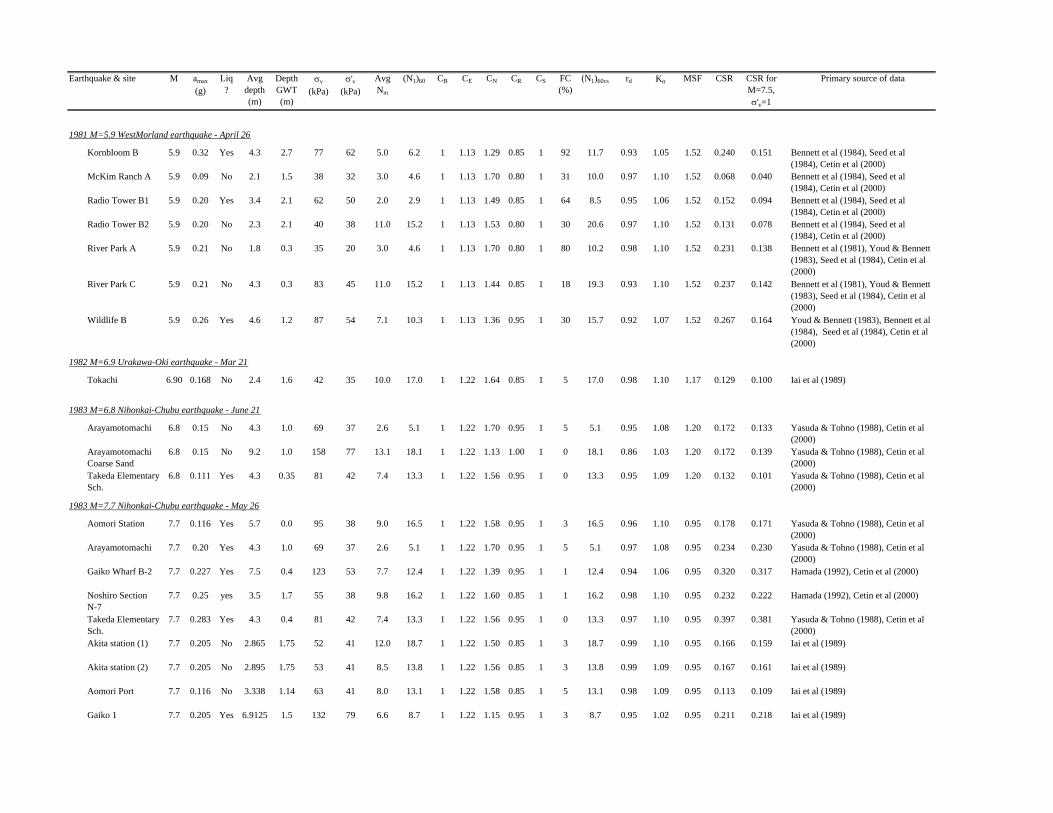
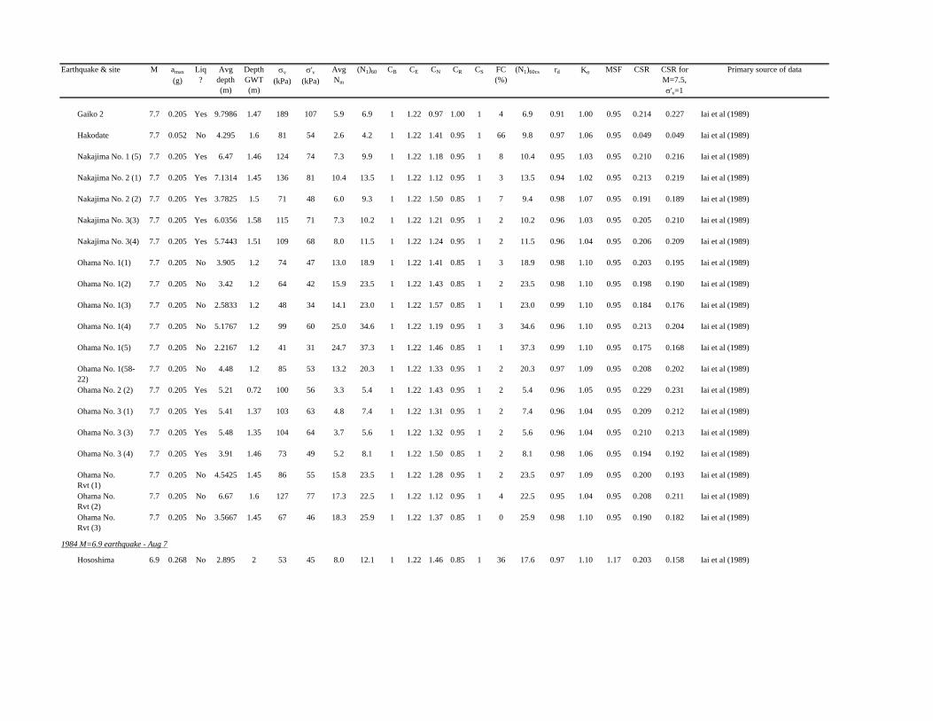
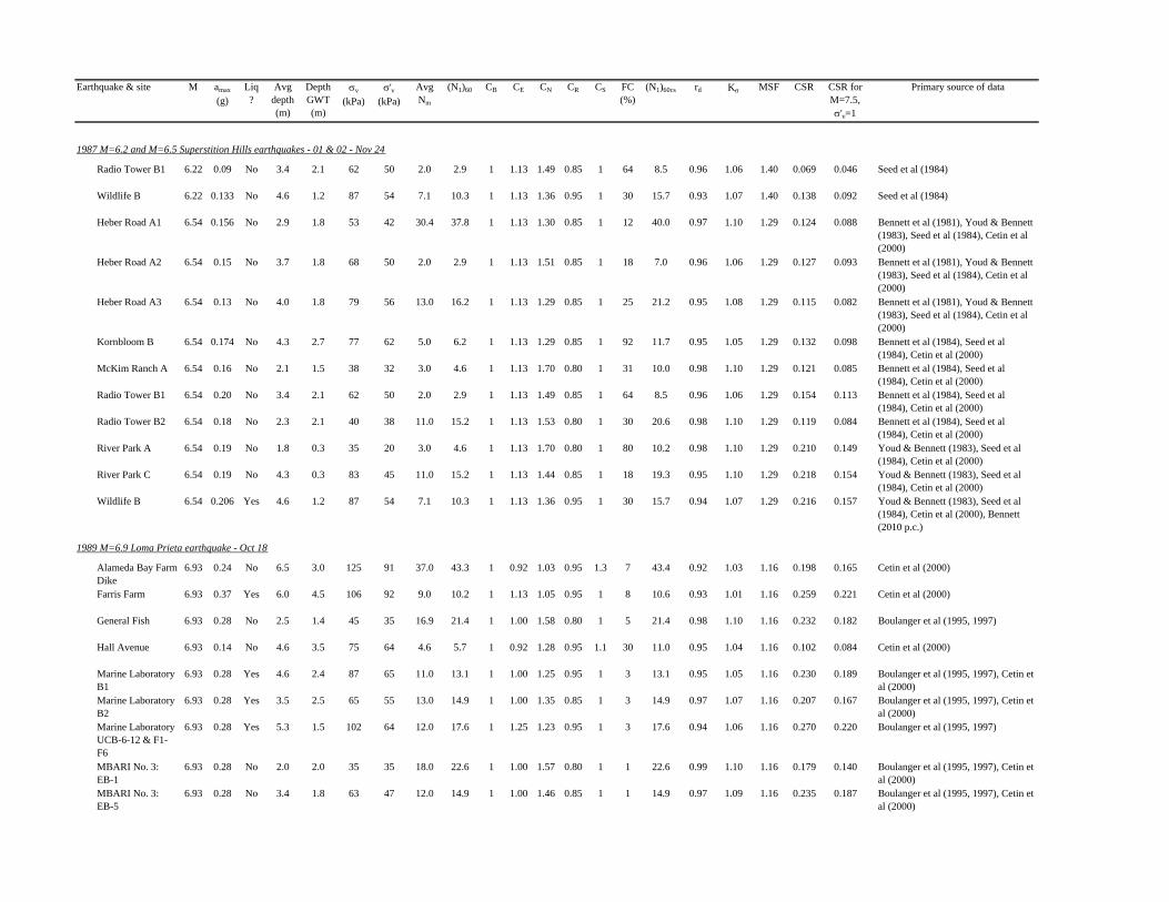
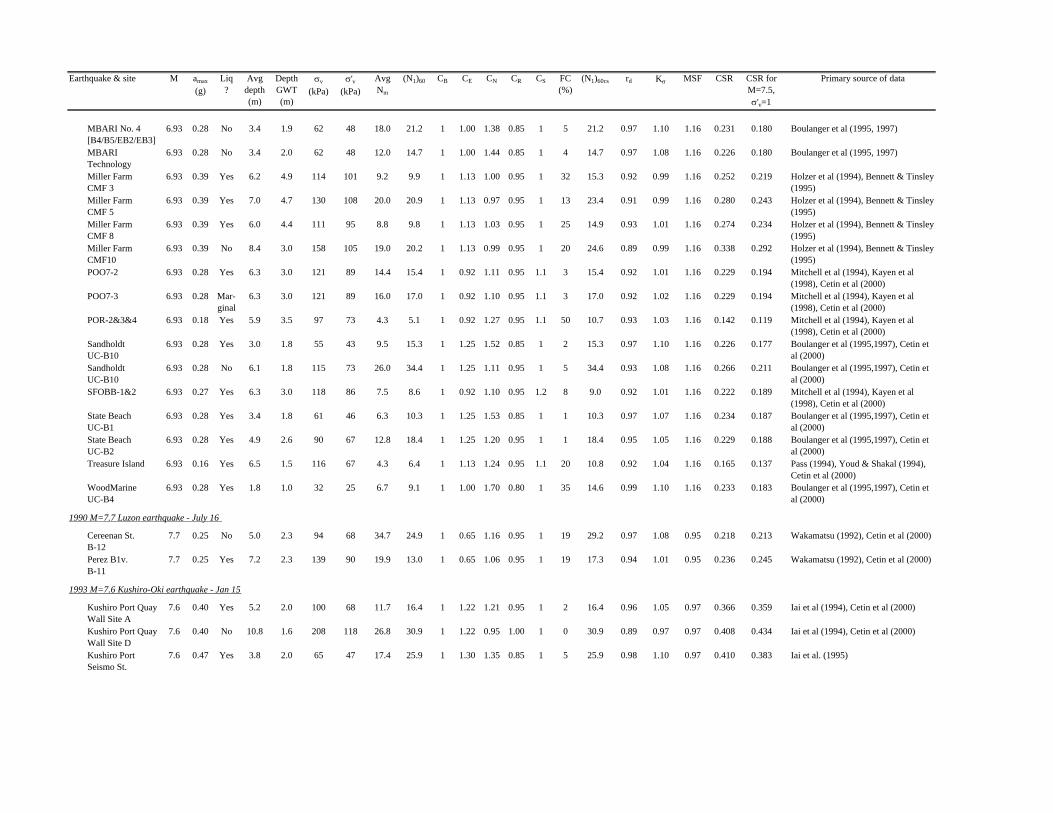
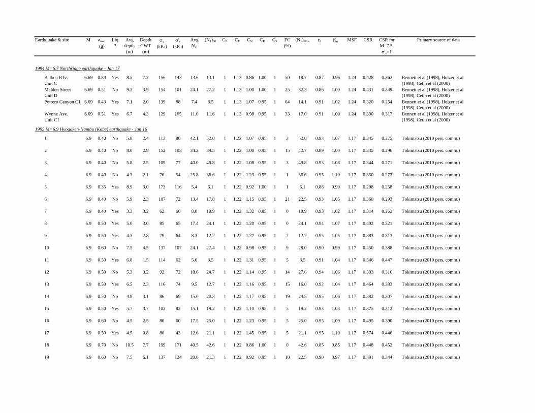
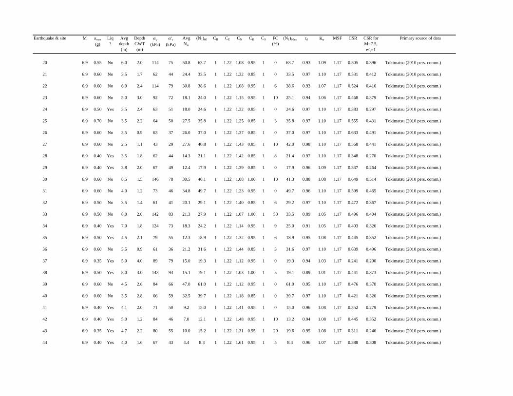
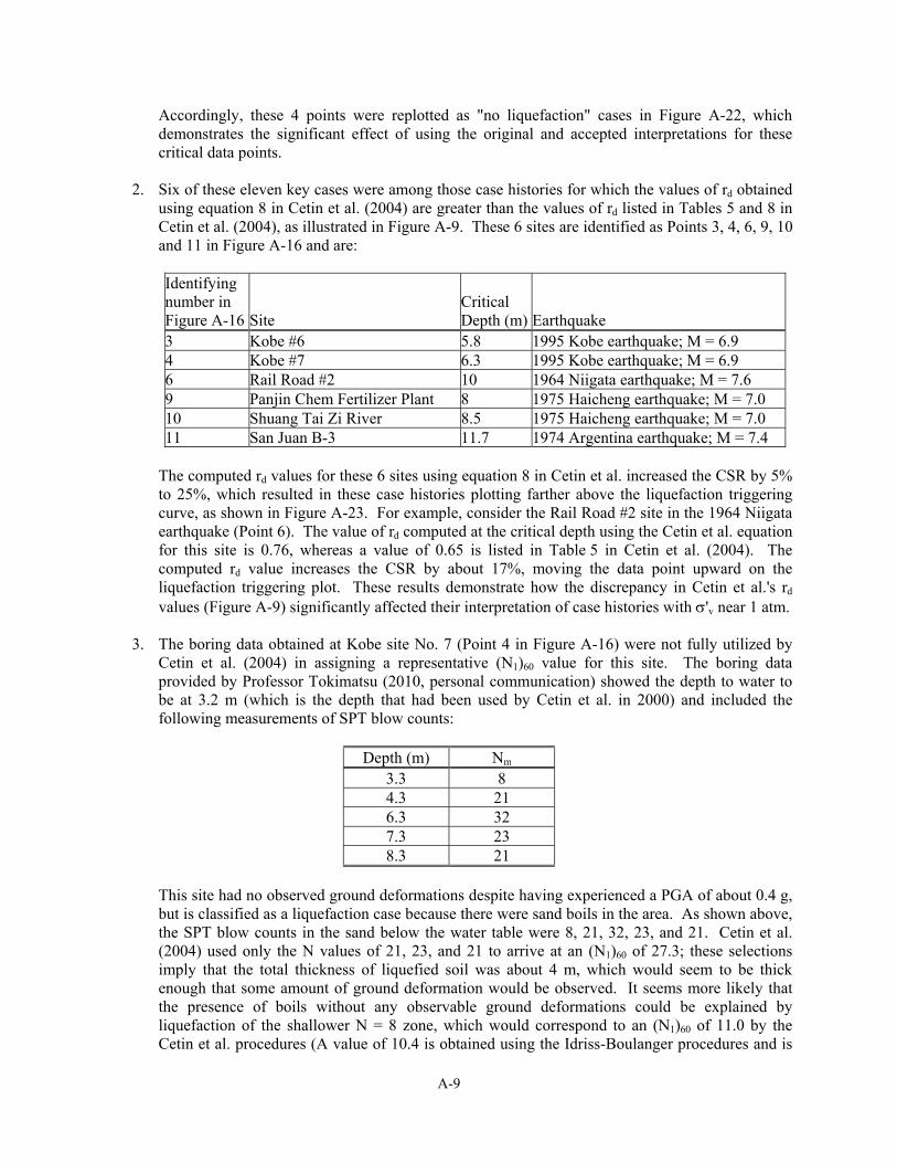
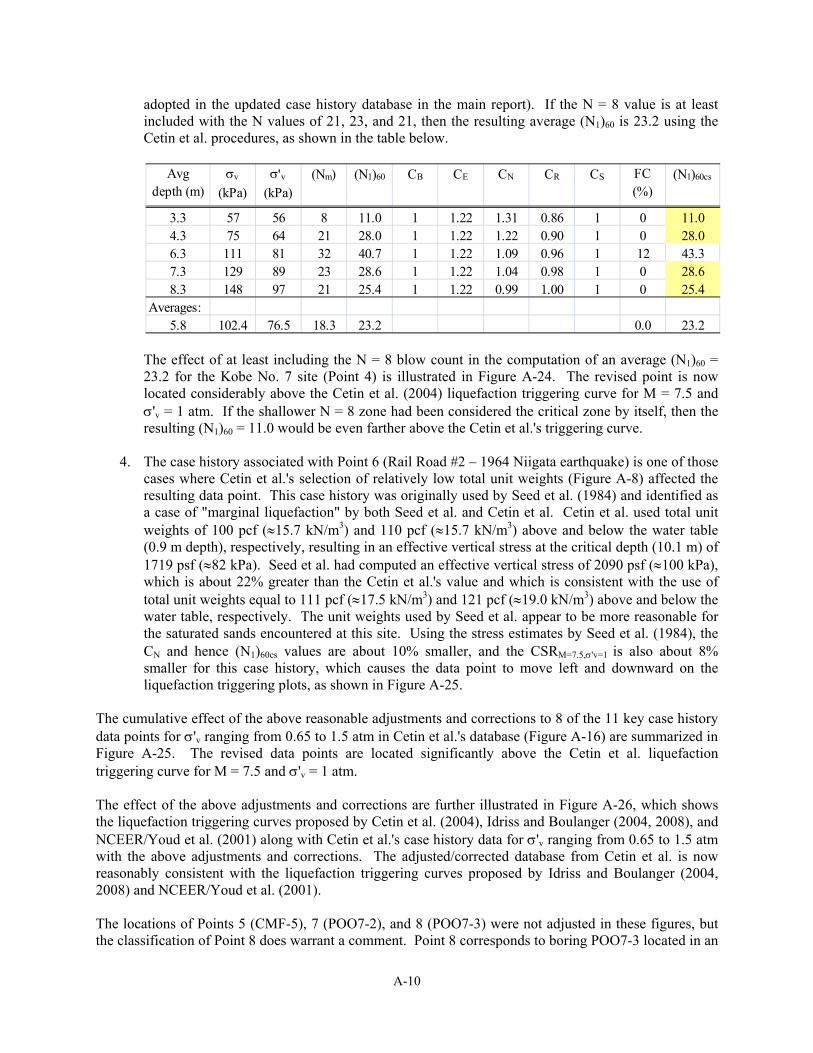
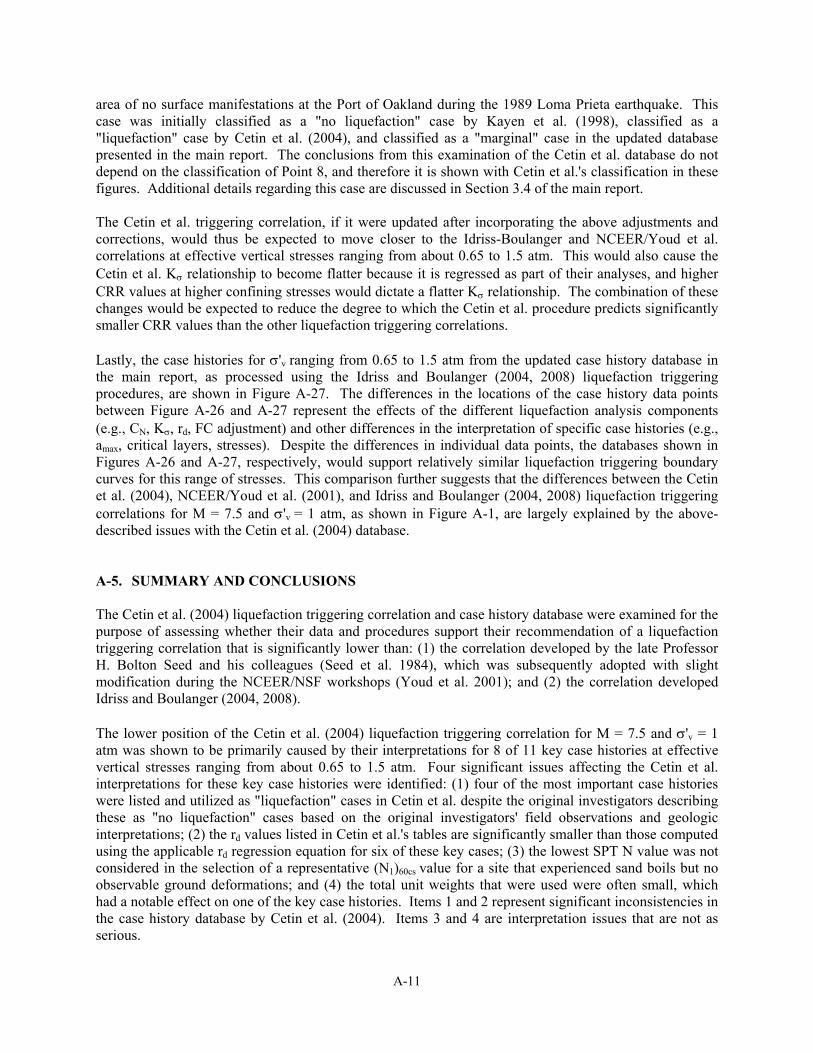
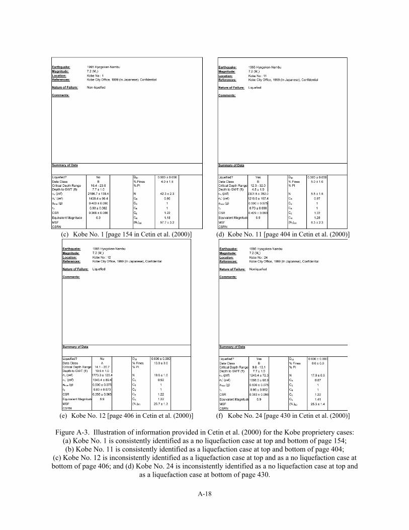
3. CASE HISTORY DATABASE 3.1. Sources of data The SPT-based case history database used to develop the Idriss and Boulanger (2004, 2008) liquefaction correlation for cohesionless soils is updated in this report, with the following specific goals: (1) incorporating additional data from Japan; (2) incorporating updated estimates of earthquake magnitudes, peak ground accelerations, and other details where improved estimates are available; (3) illustrating details of the selection and computation of SPT (N1)60cs for a number of representative case histories; and (4) presenting the distributions of the database relative to the various major parameters used in the liquefaction triggering correlation. Idriss and Boulanger (2004) primarily used cases summarized in the databases compiled by Seed et al. (1984) and Cetin et al. (2000, 2004), except that they excluded the Kobe proprietary cases that were listed in Cetin et al. (2004). Idriss and Boulanger (2004) excluded these proprietary cases because the listing of these case histories in the Cetin et al. (2004) data report contained 21 apparently inconsistent classifications (liquefied/nonliquefied) between the top and bottom of the respective summary pages (see Appendix A for additional discussion). Idriss and Boulanger considered both sets of classifications in their 2004 work, but ultimately omitted the data from their final plots due to concerns over the inconsistency in these Cetin et al. listings and the inability to review the specific details at that time. Idriss and Boulanger (2004, 2008) also primarily retained the values of critical depth, Nm, v, 'v, and the product of the correction factors CE, CR, CB and CS listed by Seed et al. for the 1984 cases and by Cetin et al. for the 2000 cases. The values for the critical depth, Nm, v, and 'v were reevaluated in the current study. The product of the correction factors CE, CR, CB and CS listed by Seed et al. for the 1984 cases and by Cetin et al. for the 2000 cases were retained in the current study, except as noted otherwise. The Fear and McRoberts (1995) database was also a helpful reference for many of the case histories. The updated database described in this report incorporates the 44 Kobe proprietary cases which were provided by Professor Kohji Tokimatsu (2010, personal communication), an additional 26 case histories summarized in Iai et al. (1989), and a small number of other additions. Data from the 1999 Kocaeli and Chi-Chi earthquakes have not yet been incorporated. The total number of case histories in the updated database is 230, of which 115 cases had surface evidence of liquefaction, 112 cases had no surface evidence of liquefaction, and 3 cases were at the margin between liquefaction and no liquefaction. The individual case histories, processed using the relationships summarized in Section 2, and the key references are summarized in Table 3.1. The following sections describe the selection of earthquake magnitudes, peak accelerations, and representative (N1)60cs values, discuss the classifications of site performance, and examine the distributions of the case history data.

Table 3.1. Summary of SPT-based liquefaction case history dataEarthquake & site M amax

(g)Liq?

Avg depth (m)

Depth GWT (m)

v

(kPa)'v

(kPa)AvgNm

(N1)60 CB CE CN CR CS FC(%)

(N1)60cs rd K MSF CSR CSR for M=7.5, 'v=1

Primary source of data

1944 M=8.1 Tohnankai earthquake - Dec 7Komei 8.1 0.20 Yes 5.2 2.1 98 68 5.9 8.2 1 1.17 1.25 0.95 1 10 9.3 0.98 1.04 0.85 0.182 0.207 Kishida (1969), Seed et al (1984),

Cetin et al (2000)Ienaga 8.1 0.20 Yes 4.3 2.4 80 61 2.3 3.4 1 1.17 1.32 0.95 1 30 8.7 0.99 1.07 0.85 0.144 0.159 Kishida (1969), Seed et al (1984),

Cetin et al (2000)Meiko 8.1 0.20 Yes 3.7 2.1 69 39 1.0 1.7 1 1.17 1.70 0.85 1 27 6.9 0.99 1.08 0.85 0.225 0.245 Kishida (1969), Seed et al (1984),

Cetin et al (2000)

1948 M=7.3 Fukui earthquake - June 28

Shonenji Temple 7.0 0.40 Yes 4.0 1.2 75 48 8.0 11.8 1 1.17 1.48 0.85 1 0 11.8 0.96 1.07 1.14 0.390 0.318 Kishida (1969), Seed et al (1984), Cetin et al (2000)

Takaya 45 7.0 0.35 Yes 7.5 3.7 141 104 17.3 21.1 1 1.30 0.99 0.95 1 4 21.1 0.90 0.99 1.14 0.283 0.251 Kishida (1969), Seed et al (1984), Cetin et al (2000)

1964 M=7.6 Niigata earthquake - June 16

Arayamotomachi 7.6 0.09 Yes 3.3 1.0 63 41 2.6 4.7 1 1.22 1.70 0.85 1 5 4.7 0.98 1.07 0.97 0.089 0.086 Yasuda & Tohno (1988), Cetin et al. (2000)

Cc17-1 7.6 0.16 Yes 7.0 0.9 132 72 8.0 9.9 1 1.09 1.20 0.95 1 2 9.9 0.94 1.03 0.97 0.179 0.178 Kishida (1966), Seed et al (1984), Cetin et al (2000)

Cc17-2 7.6 0.16 Yes 5.3 0.9 85 43 7.9 12.7 1 1.09 1.55 0.95 1 8 13.0 0.96 1.09 0.97 0.199 0.188 Kishida (1966), Seed et al (1984), Cetin et al (2000)

Kawagishi-cho 7.6 0.162 Yes 3.8 2.0 71 53 4.5 6.8 1 1.22 1.45 0.85 1 5 6.8 0.98 1.05 0.97 0.136 0.133 Ishihara & Koga (1981)

Old Town -1 7.6 0.18 No 7.0 1.8 132 81 18.0 22.7 1 1.21 1.10 0.95 1 2 22.7 0.94 1.03 0.97 0.179 0.178 Koizumi (1966), Seed et al (1984), Cetin et al (2000)

Old Town -2 7.6 0.18 No 10.1 1.8 190 109 20.0 23.5 1 1.21 0.97 1.00 1 2 23.5 0.90 0.99 0.97 0.184 0.191 Koizumi (1966), Seed et al (1984), Cetin et al (2000)

Rail Road-1 7.6 0.16 Yes 10.1 0.9 190 100 10.0 11.0 1 1.09 1.01 1.00 1 2 11.0 0.90 1.00 0.97 0.178 0.182 Koizumi (1966), Seed et al (1984), Cetin et al (2000)

Rail Road-2 7.6 0.16 Mar-ginal

10.1 0.9 190 100 16.0 17.5 1 1.09 1.01 1.00 1 2 17.5 0.90 1.00 0.97 0.178 0.182 Koizumi (1966), Seed et al (1984), Cetin et al (2000)

River Site 7.6 0.16 Yes 4.6 0.6 86 47 6.0 9.4 1 1.09 1.52 0.95 1 0 9.4 0.97 1.07 0.97 0.183 0.176 Ishihara (1979), Seed et al (1984), Cetin et al (2000)

Road Site 7.6 0.18 No 6.1 2.4 115 79 12.0 14.1 1 1.09 1.13 0.95 1 0 14.1 0.95 1.03 0.97 0.162 0.162 Ishihara (1979), Seed et al (1984), Cetin et al (2000)

Showa Br 2 7.6 0.16 Yes 4.3 0.0 80 39 4.0 7.0 1 1.09 1.70 0.95 1 10 8.2 0.97 1.08 0.97 0.210 0.199 Takada et al (1965), Seed et al (1984), Cetin et al (2000)

Showa Br 4 7.6 0.18 No 6.1 1.2 115 67 27.0 35.5 1 1.21 1.14 0.95 1 0 35.5 0.95 1.10 0.97 0.191 0.178 Takada et al (1965), Seed et al (1984), Cetin et al (2000)

1968 M=7.5 earthquake - April 1

Hososhima 7.5 0.242 No 2.895 2 53 45 8.0 12.1 1 1.22 1.46 0.85 1 36 17.6 0.98 1.10 1.00 0.185 0.168 Iai et al (1989)

Earthquake & site M amax

(g)Liq?

Avg depth (m)

Depth GWT (m)

v

(kPa)'v

(kPa)AvgNm




1968 M=8.3 Tokachi-Oki earthquake - May 16

Aomori Station 8.3 0.213 Yes 5.7 0.0 95 38 9.0 16.5 1 1.22 1.58 0.95 1 3 16.5 0.98 1.10 0.81 0.335 0.376 Yasuda & Tohno (1988), Cetin et al (2000)

Hachinohe -2 8.3 0.23 No 6.1 2.1 115 76 28.0 35.3 1 1.21 1.10 0.95 1 5 35.3 0.98 1.08 0.81 0.221 0.254 Ohsaki (1970), Seed et al. (1984), Cetin et al (2004)

Hachinohe -4 8.3 0.23 No 4.0 0.9 75 45 16.0 23.0 1 1.21 1.40 0.85 1 5 23.0 0.99 1.10 0.81 0.246 0.276 Ohsaki (1970), Seed et al. (1984), Cetin et al (2004)

Hachinohe-6 8.3 0.23 Yes 4.0 0.6 75 42 6.0 9.1 1 1.09 1.63 0.85 1 5 9.1 0.99 1.08 0.81 0.265 0.304 Ohsaki (1970), Seed et al. (1984), Cetin et al (2004)

Nanaehama1-2-3 8.3 0.20 Yes 4.0 0.9 75 45 5.0 7.6 1 1.17 1.52 0.85 1 20 12.0 0.99 1.08 0.81 0.213 0.244 Kishida (1970), Seed et al. (1984), Cetin et al (2004)

1971 M=6.6 San Fernando earthquake - Feb 9

Juvenile Hall 6.61 0.45 Yes 6.1 4.6 112 96 3.5 3.9 1 1.13 1.03 0.95 1 55 9.5 0.92 1.01 1.26 0.312 0.246 Bennett (1989), Seed et al (1984), Cetin et al (2000)

Van Norman 6.61 0.45 Yes 6.1 4.6 112 96 7.3 8.1 1 1.13 1.03 0.95 1 50 13.7 0.92 1.01 1.26 0.312 0.245 Bennett (1989), Seed et al (1984), Cetin et al (2000)

1975 M=7.0 Haicheng earthquake - Feb 4

Panjin Chemical Fertilizer Plant

7.0 0.20 Yes 8.2 1.5 155 89 9.1 7.6 1 0.83 1.07 0.95 1 67 13.2 0.89 1.01 1.14 0.203 0.175 Shengcong & Tatsuoka (1984), Seed et al (1984), Cetin et al (2000)

Shuang Tai Zi River Sluice Gate

7.0 0.20 No 8.2 1.5 158 92 9.0 8.9 1 1.00 1.05 0.95 1 50 14.6 0.89 1.01 1.14 0.199 0.172 Shengcong & Tatsuoka (1984), Seed et al (1984), Cetin et al (2000)

Ying Kou Glass Fibre Plant


Ying Kou Paper Plant


1976 M=7.5 Guatemala earthquake - Feb 4

Amatitlan B-1 7.5 0.135 Yes 10.4 1.5 139 86 6.0 5.0 1 0.75 1.10 1.00 1 3 5.0 0.89 1.01 1.00 0.126 0.125 Seed et al (1979, 1984), Cetin et al (2000)

Amatitlan B-2 7.5 0.135 Mar-ginal

4.6 2.4 55 34 8.0 9.7 1 0.75 1.70 0.95 1 3 9.7 0.97 1.10 1.00 0.138 0.126 Seed et al (1979, 1984), Cetin et al (2000)

Amatitlan B-3&4 7.5 0.135 No 10.7 3.4 137 71 16.0 14.3 1 0.75 1.19 1.00 1 3 14.3 0.89 1.04 1.00 0.149 0.144 Seed et al (1979, 1984), Cetin et al (2000)

1976 M=7.6 Tangshan earthquake - July 27

Coastal Region 7.6 0.13 Yes 4.5 1.1 87 54 9.0 11.7 1 1.00 1.37 0.95 1 12 13.8 0.97 1.06 0.97 0.130 0.125 Shengcong & Tatsuoka (1984), Seed et al (1984), Cetin et al (2000)

Le Ting L8-14 7.6 0.20 Yes 4.4 1.5 81 53 9.7 11.5 1 1.00 1.39 0.85 1 12 13.5 0.97 1.07 0.97 0.194 0.186 Shengcong & Tatsuoka (1984), Seed et al (1984), Cetin et al (2000)

Luan Nan-L1 7.6 0.22 No 3.5 1.1 62 38 19.3 24.4 1 1.00 1.49 0.85 1 5 24.4 0.98 1.10 0.97 0.226 0.211 Shengcong & Tatsuoka (1984), Seed et al (1984), Cetin et al (2000)

Luan Nan-L2 7.6 0.22 Yes 3.5 1.1 56 32 5.9 8.5 1 1.00 1.70 0.85 1 3 8.5 0.98 1.10 0.97 0.241 0.225 Shengcong & Tatsuoka (1984), Seed et al (1984), Cetin et al (2000)

Qing Jia Ying 7.6 0.35 Yes 5.3 0.9 102 59 17.0 20.1 1 1.00 1.24 0.95 1 20 24.6 0.96 1.09 0.97 0.378 0.357 Shengcong & Tatsuoka (1984), Seed et al (1984), Cetin et al (2000)

Tangshan City 7.6 0.50 No 5.3 3.1 98 75 30.0 31.6 1 1.00 1.11 0.95 1 10 32.7 0.96 1.07 0.97 0.405 0.389 Shengcong & Tatsuoka (1984), Seed et al (1984), Cetin et al (2000)


(g)Liq?

Avg depth (m)

Depth GWT (m)

v

(kPa)'v

(kPa)AvgNm




Yao Yuan Village 7.6 0.20 Yes 6.1 0.9 118 67 9.0 10.5 1 1.00 1.22 0.95 1 20 15.0 0.95 1.05 0.97 0.218 0.214 Shengcong & Tatsuoka (1984), Seed et al (1984), Cetin et al (2000)

1977 M=7.4 Argentina earthquake - Nov 23

San Juan B-1 7.5 0.20 Yes 8.2 4.6 142 106 9.0 6.3 1 0.75 0.97 0.95 1 20 10.7 0.92 1.00 1.00 0.160 0.161 Idriss et al (1979), Seed et al (1984), Cetin et al (2000)


San Juan B-4 7.5 0.20 No 3.7 1.2 63 39 14.0 14.3 1 0.75 1.60 0.85 1 4 14.3 0.98 1.10 1.00 0.204 0.186 Idriss et al (1979), Seed et al (1984), Cetin et al (2000)

San Juan B-5 7.5 0.20 No 3.1 2.1 53 44 14.0 13.6 1 0.75 1.53 0.85 1 3 13.6 0.98 1.09 1.00 0.154 0.142 Idriss et al (1979), Seed et al (1984), Cetin et al (2000)


1978 M=6.5 Miyagiken-Oki earthquake - Feb 20

Arahama (A-9) 6.5 0.10 No 6.4 0.9 121 67 10.0 12.8 1 1.09 1.23 0.95 1 0 12.8 0.90 1.04 1.34 0.105 0.076 Tohno & Yasuda (1981), Seed et al (1984), Cetin et al (2000)

Hiyori-18 (site C)

6.5 0.14 No 5.2 2.4 98 71 9.0 11.1 1 1.09 1.19 0.95 1 20 15.5 0.93 1.04 1.34 0.116 0.084 Tsuchida et al (1980), Seed et al (1984), Cetin et al (2000)

Ishinomaki-2 6.5 0.12 No 3.5 1.4 66 45 3.7 5.5 1 1.09 1.61 0.85 1 10 6.7 0.96 1.07 1.34 0.109 0.076 Ishihara et al (1980), Seed et al (1984), Cetin et al (2000)

Kitawabuchi-2 6.5 0.14 No 3.4 3.1 62 59 11.0 12.3 1 1.00 1.32 0.85 1 5 12.3 0.96 1.05 1.34 0.092 0.065 Iwasaki et al (1981), Seed et al (1984), Cetin et al (2000)

Nakajima-18 (Site A)

6.5 0.14 No 6.1 2.4 115 79 12.0 14.1 1 1.09 1.13 0.95 1 3 14.1 0.91 1.03 1.34 0.120 0.088 Tsuchida et al (1979, 1980), Tohno & Yasuda (1981), Seed et al (1984), Cetin et al (2000)

Nakamura Dyke N-4

6.5 0.12 Yes 2.8 0.5 53 30 4.7 6.9 1 1.00 1.70 0.85 1 5 6.9 0.97 1.10 1.34 0.128 0.087 Iwasaki & Tokida (1980), Tohno & Yasuda (1981), Seed et al (1984), Cetin et al (2000)

Nakamura Dyke N-5

6.5 0.12 No 3.4 1.3 63 42 7.0 9.6 1 1.00 1.61 0.85 1 4 9.6 0.96 1.08 1.34 0.112 0.078 Iwasaki & Tokida (1980), Tohno & Yasuda (1981), Seed et al (1984), Cetin et al (2000)

Oiiri-1 6.5 0.14 No 6.4 4.3 106 85 9.0 9.4 1 1.00 1.10 0.95 1 5 9.4 0.90 1.02 1.34 0.102 0.075 Iwasaki et al (1978), Tohno & Yasuda (1981), Seed et al (1984), Cetin et al (2000)

Shiomi-6 (Site D) 6.5 0.14 No 4.0 2.4 75 60 6.0 7.5 1 1.09 1.34 0.85 1 10 8.6 0.95 1.05 1.34 0.108 0.077 Tsuchida et al (1979, 1980), Tohno & Yasuda (1981), Tokimatsu (1983), Seed et al (1984), Cetin et al (2000)

Yuriage Br-1 6.5 0.12 No 4.3 1.8 80 56 4.0 5.4 1 1.00 1.41 0.95 1 10 6.5 0.94 1.05 1.34 0.105 0.075 Iwasaki et al (1978), Tohno & Yasuda (1981), Seed et al (1984), Cetin et al (2000)




(g)Liq?

Avg depth (m)

Depth GWT (m)

v

(kPa)'v

(kPa)AvgNm




Yuriagekami-1 6.5 0.12 No 5.5 1.8 99 63 2.0 2.5 1 1.00 1.31 0.95 1 60 8.1 0.92 1.04 1.34 0.113 0.081 Iwasaki et al (1984), Tohno & Yasuda (1981), Seed et al (1984), Cetin et al (2000)

Yuriagekami-2 6.5 0.12 No 4.3 0.9 80 47 11.0 15.1 1 1.00 1.45 0.95 1 0 15.1 0.94 1.08 1.34 0.125 0.086 Iwasaki et al (1984), Tohno & Yasuda (1981), Seed et al (1984), Cetin et al (2000)

1978 M=7.7 Miyagiken-Oki earthquake - June 12

Arahama (A-9) 7.7 0.20 Yes 6.4 0.9 121 67 10.0 12.8 1 1.09 1.23 0.95 1 0 12.8 0.95 1.04 0.95 0.223 0.225 Tohno & Yasuda (1981), Seed et al (1984), Cetin et al (2000)

Hiyori-18 (site C)

7.7 0.24 Yes 5.2 2.4 98 71 9.0 11.1 1 1.09 1.19 0.95 1 20 15.5 0.96 1.04 0.95 0.207 0.210 Tsuchida et al (1979, 1980), Seed et al (1984), Cetin et al (2000)

Ishinomaki-2 7.7 0.20 Yes 3.5 1.4 66 45 3.7 5.5 1 1.09 1.61 0.85 1 10 6.7 0.98 1.07 0.95 0.186 0.184 Ishihara et al (1980), Seed et al (1984), Cetin et al (2000)

Ishinomaki-4 7.7 0.20 No 4.5 1.4 87 57 14.2 20.9 1 1.21 1.28 0.95 1 10 22.0 0.97 1.08 0.95 0.188 0.183 Ishihara et al (1980), Seed et al (1984), Cetin et al (2000)

Kitawabuchi-2 7.7 0.28 Yes 3.4 3.1 62 59 11.0 12.3 1 1.00 1.32 0.85 1 5 12.3 0.98 1.05 0.95 0.187 0.187 Iwasaki et al (1981), Tohno & Yasuda (1981), Seed et al (1984), Cetin et al (2000)

Kitawabuchi-3 7.7 0.28 No 4.8 3.1 90 73 13.2 17.6 1 1.21 1.16 0.95 1 0 17.6 0.97 1.04 0.95 0.216 0.220 Iwasaki et al (1981), Tohno & Yasuda (1981), Seed et al (1984), Cetin et al (2000)

Nakajima 2 7.7 0.24 No 4.6 2.4 86 65 10.0 12.7 1 1.09 1.23 0.95 1 26 17.8 0.97 1.05 0.95 0.200 0.200 Tsuchida et al (1979, 1980), Tohno & Yasuda (1981), Seed et al (1984), Cetin et al (2000)

Nakajima-18 (Site A)

7.7 0.24 Yes 6.1 2.4 115 79 12.0 14.1 1 1.09 1.13 0.95 1 3 14.1 0.96 1.03 0.95 0.217 0.223 Tsuchida et al (1979, 1980), Seed et al (1984), Cetin et al (2000)

Nakamura Dyke N-1

7.7 0.32 No 3.4 0.9 63 39 19.0 26.2 1 1.12 1.45 0.85 1 4 26.2 0.98 1.10 0.95 0.329 0.315 Iwasaki & Tokida (1980), Tohno & Yasuda (1981), Seed et al (1984), Cetin et al (2000)

Nakamura Dyke N-4

7.7 0.32 Yes 2.8 0.5 53 30 4.7 6.9 1 1.00 1.70 0.85 1 5 6.9 0.99 1.10 0.95 0.346 0.332 Iwasaki (1986), Tohno & Yasuda (1981), Seed et al (1984), Cetin et al (2000)

Nakamura Dyke N-5

7.7 0.32 Yes 3.4 1.3 63 42 7.0 9.6 1 1.00 1.61 0.85 1 4 9.6 0.98 1.08 0.95 0.306 0.299 Iwasaki (1986), Tohno & Yasuda (1981), Seed et al (1984), Cetin et al (2000)

Oiiri-1 7.7 0.24 Yes 6.4 4.3 106 85 9.0 9.4 1 1.00 1.10 0.95 1 5 9.4 0.95 1.02 0.95 0.185 0.192 Iwasaki et al (1978), Tohno & Yasuda (1981), Seed et al (1984), Cetin et al (2000)

Shiomi-6 (Site D) 7.7 0.24 Yes 4.0 2.4 75 60 6.0 7.5 1 1.09 1.34 0.85 1 10 8.6 0.98 1.05 0.95 0.190 0.192 Tsuchida et al (1979, 1980), Tohno & Yasuda (1981), Tokimatsu (1983), Seed et al (1984), Cetin et al (2000)

Yuriage Br-1 7.7 0.24 Yes 4.3 1.8 80 56 4.0 5.4 1 1.00 1.41 0.95 1 10 6.5 0.97 1.05 0.95 0.216 0.218 Iwasaki et al (1978), Tohno & Yasuda (1981), Seed et al (1984), Cetin et al (2000)



(g)Liq?

Avg depth (m)

Depth GWT (m)

v

(kPa)'v

(kPa)AvgNm






Yuriagekami-1 7.7 0.24 Yes 5.5 1.8 99 63 2.0 2.5 1 1.00 1.31 0.95 1 60 8.1 0.96 1.04 0.95 0.236 0.239 Iwasaki & Tokida (1980), Iwasaki et al (1984), Tohno & Yasuda (1981), Seed et al (1984), Cetin et al (2000)

Yuriagekami-2 7.7 0.24 Yes 4.3 0.9 80 47 11.0 15.1 1 1.00 1.45 0.95 1 0 15.1 0.97 1.08 0.95 0.258 0.251 Iwasaki & Tokida (1980), Iwasaki et al (1984), Tohno & Yasuda (1981), Seed et al (1984), Cetin et al (2000)

Yuriagekami-3 7.7 0.24 No 5.5 2.1 103 70 20.0 24.6 1 1.12 1.16 0.95 1 0 24.6 0.96 1.06 0.95 0.220 0.220 Iwasaki & Tokida (1980), Iwasaki et al (1984), Tohno & Yasuda (1981), Seed et al (1984), Cetin et al (2000)

1979 ML=6.5 Imperial Valley earthquake - Oct 15

Heber Road A1 6.53 0.78 No 2.9 1.8 53 42 30.4 37.8 1 1.13 1.30 0.85 1 12 40.0 0.97 1.10 1.29 0.620 0.437 Bennett et al (1981), Youd & Bennett (1983), Seed et al (1984), Cetin et al (2000)

Heber Road A2 6.53 0.78 Yes 3.7 1.8 68 50 2.0 2.9 1 1.13 1.51 0.85 1 18 7.0 0.96 1.06 1.29 0.661 0.484 Bennett et al (1981), Youd & Bennett (1983), Seed et al (1984), Cetin et al (2000)


Kornbloom B 6.53 0.13 No 4.3 2.7 77 62 5.0 6.2 1 1.13 1.29 0.85 1 92 11.7 0.95 1.05 1.29 0.099 0.073 Bennett et al (1984), Seed et al (1984), Cetin et al (2000)

McKim Ranch A 6.53 0.51 Yes 2.1 1.5 38 32 3.0 4.6 1 1.13 1.70 0.80 1 31 10.0 0.98 1.10 1.29 0.385 0.271 Bennett et al (1984), Seed et al (1984), Cetin et al (2000)

Radio Tower B1 6.53 0.20 Yes 3.4 2.1 62 50 2.0 2.9 1 1.13 1.49 0.85 1 64 8.5 0.96 1.06 1.29 0.154 0.112 Bennett et al (1984), Seed et al (1984), Cetin et al (2000)

Radio Tower B2 6.53 0.20 No 2.3 2.1 40 38 11.0 15.2 1 1.13 1.53 0.80 1 30 20.6 0.98 1.10 1.29 0.132 0.093 Bennett et al (1984), Seed et al (1984), Cetin et al (2000)

River Park A 6.53 0.24 Yes 1.8 0.3 35 20 3.0 4.6 1 1.13 1.70 0.80 1 80 10.2 0.98 1.10 1.29 0.266 0.187 Bennett et al (1981), Youd & Bennett (1983), Seed et al (1984), Cetin et al (2000)

Wildlife B 6.53 0.17 No 4.6 1.2 87 54 7.1 10.3 1 1.13 1.36 0.95 1 30 15.7 0.94 1.07 1.29 0.178 0.129 Youd & Bennett (1983), Bennett et al (1984), Seed et al (1984), Cetin et al (2000)

1980 M=6.0 Mid-Chiba earthquake - Sept 24 (UTC)

Owi-1 6.0 0.095 No 6.1 0.9 108 57 5.0 7.1 1 1.09 1.36 0.95 1 13 9.6 0.89 1.05 1.48 0.104 0.067 Ishihara et al (1981), Seed et al (1984), Cetin et al (2000)

Owi-2 6.0 0.095 No 14.3 0.9 254 123 4.0 3.9 1 1.09 0.90 1.00 1 27 9.1 0.69 0.98 1.48 0.089 0.061 Ishihara et al (1981), Seed et al (1984), Cetin et al (2000)


(g)Liq?

Avg depth (m)

Depth GWT (m)

v

(kPa)'v

(kPa)AvgNm




1981 M=5.9 WestMorland earthquake - April 26

Kornbloom B 5.9 0.32 Yes 4.3 2.7 77 62 5.0 6.2 1 1.13 1.29 0.85 1 92 11.7 0.93 1.05 1.52 0.240 0.151 Bennett et al (1984), Seed et al (1984), Cetin et al (2000)

McKim Ranch A 5.9 0.09 No 2.1 1.5 38 32 3.0 4.6 1 1.13 1.70 0.80 1 31 10.0 0.97 1.10 1.52 0.068 0.040 Bennett et al (1984), Seed et al (1984), Cetin et al (2000)

Radio Tower B1 5.9 0.20 Yes 3.4 2.1 62 50 2.0 2.9 1 1.13 1.49 0.85 1 64 8.5 0.95 1.06 1.52 0.152 0.094 Bennett et al (1984), Seed et al (1984), Cetin et al (2000)


River Park A 5.9 0.21 No 1.8 0.3 35 20 3.0 4.6 1 1.13 1.70 0.80 1 80 10.2 0.98 1.10 1.52 0.231 0.138 Bennett et al (1981), Youd & Bennett (1983), Seed et al (1984), Cetin et al (2000)

River Park C 5.9 0.21 No 4.3 0.3 83 45 11.0 15.2 1 1.13 1.44 0.85 1 18 19.3 0.93 1.10 1.52 0.237 0.142 Bennett et al (1981), Youd & Bennett (1983), Seed et al (1984), Cetin et al (2000)

Wildlife B 5.9 0.26 Yes 4.6 1.2 87 54 7.1 10.3 1 1.13 1.36 0.95 1 30 15.7 0.92 1.07 1.52 0.267 0.164 Youd & Bennett (1983), Bennett et al (1984), Seed et al (1984), Cetin et al (2000)

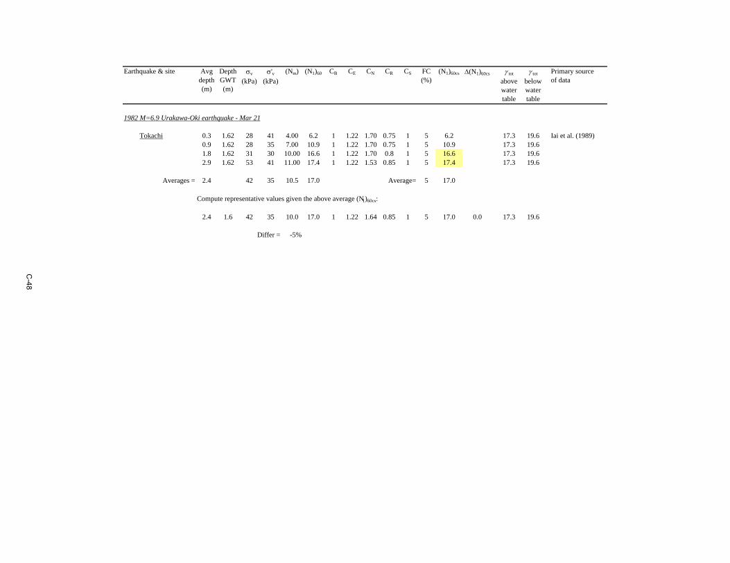
1982 M=6.9 Urakawa-Oki earthquake - Mar 21

Tokachi 6.90 0.168 No 2.4 1.6 42 35 10.0 17.0 1 1.22 1.64 0.85 1 5 17.0 0.98 1.10 1.17 0.129 0.100 Iai et al (1989)

1983 M=6.8 Nihonkai-Chubu earthquake - June 21

Arayamotomachi 6.8 0.15 No 4.3 1.0 69 37 2.6 5.1 1 1.22 1.70 0.95 1 5 5.1 0.95 1.08 1.20 0.172 0.133 Yasuda & Tohno (1988), Cetin et al (2000)

Arayamotomachi Coarse Sand

6.8 0.15 No 9.2 1.0 158 77 13.1 18.1 1 1.22 1.13 1.00 1 0 18.1 0.86 1.03 1.20 0.172 0.139 Yasuda & Tohno (1988), Cetin et al (2000)

Takeda Elementary Sch.

6.8 0.111 Yes 4.3 0.35 81 42 7.4 13.3 1 1.22 1.56 0.95 1 0 13.3 0.95 1.09 1.20 0.132 0.101 Yasuda & Tohno (1988), Cetin et al (2000)

1983 M=7.7 Nihonkai-Chubu earthquake - May 26

Aomori Station 7.7 0.116 Yes 5.7 0.0 95 38 9.0 16.5 1 1.22 1.58 0.95 1 3 16.5 0.96 1.10 0.95 0.178 0.171 Yasuda & Tohno (1988), Cetin et al (2000)

Arayamotomachi 7.7 0.20 Yes 4.3 1.0 69 37 2.6 5.1 1 1.22 1.70 0.95 1 5 5.1 0.97 1.08 0.95 0.234 0.230 Yasuda & Tohno (1988), Cetin et al (2000)

Gaiko Wharf B-2 7.7 0.227 Yes 7.5 0.4 123 53 7.7 12.4 1 1.22 1.39 0.95 1 1 12.4 0.94 1.06 0.95 0.320 0.317 Hamada (1992), Cetin et al (2000)

Noshiro Section N-7

7.7 0.25 yes 3.5 1.7 55 38 9.8 16.2 1 1.22 1.60 0.85 1 1 16.2 0.98 1.10 0.95 0.232 0.222 Hamada (1992), Cetin et al (2000)


7.7 0.283 Yes 4.3 0.4 81 42 7.4 13.3 1 1.22 1.56 0.95 1 0 13.3 0.97 1.10 0.95 0.397 0.381 Yasuda & Tohno (1988), Cetin et al (2000)

Akita station (1) 7.7 0.205 No 2.865 1.75 52 41 12.0 18.7 1 1.22 1.50 0.85 1 3 18.7 0.99 1.10 0.95 0.166 0.159 Iai et al (1989)

Akita station (2) 7.7 0.205 No 2.895 1.75 53 41 8.5 13.8 1 1.22 1.56 0.85 1 3 13.8 0.99 1.09 0.95 0.167 0.161 Iai et al (1989)

Aomori Port 7.7 0.116 No 3.338 1.14 63 41 8.0 13.1 1 1.22 1.58 0.85 1 5 13.1 0.98 1.09 0.95 0.113 0.109 Iai et al (1989)

Gaiko 1 7.7 0.205 Yes 6.9125 1.5 132 79 6.6 8.7 1 1.22 1.15 0.95 1 3 8.7 0.95 1.02 0.95 0.211 0.218 Iai et al (1989)


(g)Liq?

Avg depth (m)

Depth GWT (m)

v

(kPa)'v

(kPa)AvgNm




Gaiko 2 7.7 0.205 Yes 9.7986 1.47 189 107 5.9 6.9 1 1.22 0.97 1.00 1 4 6.9 0.91 1.00 0.95 0.214 0.227 Iai et al (1989)

Hakodate 7.7 0.052 No 4.295 1.6 81 54 2.6 4.2 1 1.22 1.41 0.95 1 66 9.8 0.97 1.06 0.95 0.049 0.049 Iai et al (1989)

Nakajima No. 1 (5) 7.7 0.205 Yes 6.47 1.46 124 74 7.3 9.9 1 1.22 1.18 0.95 1 8 10.4 0.95 1.03 0.95 0.210 0.216 Iai et al (1989)



Nakajima No. 3(3) 7.7 0.205 Yes 6.0356 1.58 115 71 7.3 10.2 1 1.22 1.21 0.95 1 2 10.2 0.96 1.03 0.95 0.205 0.210 Iai et al (1989)

Nakajima No. 3(4) 7.7 0.205 Yes 5.7443 1.51 109 68 8.0 11.5 1 1.22 1.24 0.95 1 2 11.5 0.96 1.04 0.95 0.206 0.209 Iai et al (1989)

Ohama No. 1(1) 7.7 0.205 No 3.905 1.2 74 47 13.0 18.9 1 1.22 1.41 0.85 1 3 18.9 0.98 1.10 0.95 0.203 0.195 Iai et al (1989)





Ohama No. 1(58-22)

7.7 0.205 No 4.48 1.2 85 53 13.2 20.3 1 1.22 1.33 0.95 1 2 20.3 0.97 1.09 0.95 0.208 0.202 Iai et al (1989)

Ohama No. 2 (2) 7.7 0.205 Yes 5.21 0.72 100 56 3.3 5.4 1 1.22 1.43 0.95 1 2 5.4 0.96 1.05 0.95 0.229 0.231 Iai et al (1989)




Ohama No. Rvt (1)

7.7 0.205 No 4.5425 1.45 86 55 15.8 23.5 1 1.22 1.28 0.95 1 2 23.5 0.97 1.09 0.95 0.200 0.193 Iai et al (1989)

Ohama No. Rvt (2)

7.7 0.205 No 6.67 1.6 127 77 17.3 22.5 1 1.22 1.12 0.95 1 4 22.5 0.95 1.04 0.95 0.208 0.211 Iai et al (1989)

Ohama No. Rvt (3)

7.7 0.205 No 3.5667 1.45 67 46 18.3 25.9 1 1.22 1.37 0.85 1 0 25.9 0.98 1.10 0.95 0.190 0.182 Iai et al (1989)

1984 M=6.9 earthquake - Aug 7

Hososhima 6.9 0.268 No 2.895 2 53 45 8.0 12.1 1 1.22 1.46 0.85 1 36 17.6 0.97 1.10 1.17 0.203 0.158 Iai et al (1989)


(g)Liq?

Avg depth (m)

Depth GWT (m)

v

(kPa)'v

(kPa)AvgNm




1987 M=6.2 and M=6.5 Superstition Hills earthquakes - 01 & 02 - Nov 24

Radio Tower B1 6.22 0.09 No 3.4 2.1 62 50 2.0 2.9 1 1.13 1.49 0.85 1 64 8.5 0.96 1.06 1.40 0.069 0.046 Seed et al (1984)

Wildlife B 6.22 0.133 No 4.6 1.2 87 54 7.1 10.3 1 1.13 1.36 0.95 1 30 15.7 0.93 1.07 1.40 0.138 0.092 Seed et al (1984)




Kornbloom B 6.54 0.174 No 4.3 2.7 77 62 5.0 6.2 1 1.13 1.29 0.85 1 92 11.7 0.95 1.05 1.29 0.132 0.098 Bennett et al (1984), Seed et al (1984), Cetin et al (2000)

McKim Ranch A 6.54 0.16 No 2.1 1.5 38 32 3.0 4.6 1 1.13 1.70 0.80 1 31 10.0 0.98 1.10 1.29 0.121 0.085 Bennett et al (1984), Seed et al (1984), Cetin et al (2000)



River Park A 6.54 0.19 No 1.8 0.3 35 20 3.0 4.6 1 1.13 1.70 0.80 1 80 10.2 0.98 1.10 1.29 0.210 0.149 Youd & Bennett (1983), Seed et al (1984), Cetin et al (2000)

River Park C 6.54 0.19 No 4.3 0.3 83 45 11.0 15.2 1 1.13 1.44 0.85 1 18 19.3 0.95 1.10 1.29 0.218 0.154 Youd & Bennett (1983), Seed et al (1984), Cetin et al (2000)

Wildlife B 6.54 0.206 Yes 4.6 1.2 87 54 7.1 10.3 1 1.13 1.36 0.95 1 30 15.7 0.94 1.07 1.29 0.216 0.157 Youd & Bennett (1983), Seed et al (1984), Cetin et al (2000), Bennett (2010 p.c.)

1989 M=6.9 Loma Prieta earthquake - Oct 18

Alameda Bay Farm Dike

6.93 0.24 No 6.5 3.0 125 91 37.0 43.3 1 0.92 1.03 0.95 1.3 7 43.4 0.92 1.03 1.16 0.198 0.165 Cetin et al (2000)

Farris Farm 6.93 0.37 Yes 6.0 4.5 106 92 9.0 10.2 1 1.13 1.05 0.95 1 8 10.6 0.93 1.01 1.16 0.259 0.221 Cetin et al (2000)

General Fish 6.93 0.28 No 2.5 1.4 45 35 16.9 21.4 1 1.00 1.58 0.80 1 5 21.4 0.98 1.10 1.16 0.232 0.182 Boulanger et al (1995, 1997)

Hall Avenue 6.93 0.14 No 4.6 3.5 75 64 4.6 5.7 1 0.92 1.28 0.95 1.1 30 11.0 0.95 1.04 1.16 0.102 0.084 Cetin et al (2000)

Marine Laboratory B1

6.93 0.28 Yes 4.6 2.4 87 65 11.0 13.1 1 1.00 1.25 0.95 1 3 13.1 0.95 1.05 1.16 0.230 0.189 Boulanger et al (1995, 1997), Cetin et al (2000)

Marine Laboratory B2

6.93 0.28 Yes 3.5 2.5 65 55 13.0 14.9 1 1.00 1.35 0.85 1 3 14.9 0.97 1.07 1.16 0.207 0.167 Boulanger et al (1995, 1997), Cetin et al (2000)

Marine Laboratory UCB-6-12 & F1-F6

6.93 0.28 Yes 5.3 1.5 102 64 12.0 17.6 1 1.25 1.23 0.95 1 3 17.6 0.94 1.06 1.16 0.270 0.220 Boulanger et al (1995, 1997)

MBARI No. 3: EB-1

6.93 0.28 No 2.0 2.0 35 35 18.0 22.6 1 1.00 1.57 0.80 1 1 22.6 0.99 1.10 1.16 0.179 0.140 Boulanger et al (1995, 1997), Cetin et al (2000)

MBARI No. 3: EB-5

6.93 0.28 No 3.4 1.8 63 47 12.0 14.9 1 1.00 1.46 0.85 1 1 14.9 0.97 1.09 1.16 0.235 0.187 Boulanger et al (1995, 1997), Cetin et al (2000)


(g)Liq?

Avg depth (m)

Depth GWT (m)

v

(kPa)'v

(kPa)AvgNm




MBARI No. 4 [B4/B5/EB2/EB3]

6.93 0.28 No 3.4 1.9 62 48 18.0 21.2 1 1.00 1.38 0.85 1 5 21.2 0.97 1.10 1.16 0.231 0.180 Boulanger et al (1995, 1997)

MBARI Technology

6.93 0.28 No 3.4 2.0 62 48 12.0 14.7 1 1.00 1.44 0.85 1 4 14.7 0.97 1.08 1.16 0.226 0.180 Boulanger et al (1995, 1997)

Miller Farm CMF 3

6.93 0.39 Yes 6.2 4.9 114 101 9.2 9.9 1 1.13 1.00 0.95 1 32 15.3 0.92 0.99 1.16 0.252 0.219 Holzer et al (1994), Bennett & Tinsley (1995)

Miller Farm CMF 5


Miller Farm CMF 8


Miller Farm CMF10

6.93 0.39 No 8.4 3.0 158 105 19.0 20.2 1 1.13 0.99 0.95 1 20 24.6 0.89 0.99 1.16 0.338 0.292 Holzer et al (1994), Bennett & Tinsley (1995)

POO7-2 6.93 0.28 Yes 6.3 3.0 121 89 14.4 15.4 1 0.92 1.11 0.95 1.1 3 15.4 0.92 1.01 1.16 0.229 0.194 Mitchell et al (1994), Kayen et al (1998), Cetin et al (2000)

POO7-3 6.93 0.28 Mar-ginal

6.3 3.0 121 89 16.0 17.0 1 0.92 1.10 0.95 1.1 3 17.0 0.92 1.02 1.16 0.229 0.194 Mitchell et al (1994), Kayen et al (1998), Cetin et al (2000)

POR-2&3&4 6.93 0.18 Yes 5.9 3.5 97 73 4.3 5.1 1 0.92 1.27 0.95 1.1 50 10.7 0.93 1.03 1.16 0.142 0.119 Mitchell et al (1994), Kayen et al (1998), Cetin et al (2000)

Sandholdt UC-B10

6.93 0.28 Yes 3.0 1.8 55 43 9.5 15.3 1 1.25 1.52 0.85 1 2 15.3 0.97 1.10 1.16 0.226 0.177 Boulanger et al (1995,1997), Cetin et al (2000)

Sandholdt UC-B10

6.93 0.28 No 6.1 1.8 115 73 26.0 34.4 1 1.25 1.11 0.95 1 5 34.4 0.93 1.08 1.16 0.266 0.211 Boulanger et al (1995,1997), Cetin et al (2000)

SFOBB-1&2 6.93 0.27 Yes 6.3 3.0 118 86 7.5 8.6 1 0.92 1.10 0.95 1.2 8 9.0 0.92 1.01 1.16 0.222 0.189 Mitchell et al (1994), Kayen et al (1998), Cetin et al (2000)

State Beach UC-B1


State Beach UC-B2


Treasure Island 6.93 0.16 Yes 6.5 1.5 116 67 4.3 6.4 1 1.13 1.24 0.95 1.1 20 10.8 0.92 1.04 1.16 0.165 0.137 Pass (1994), Youd & Shakal (1994), Cetin et al (2000)

WoodMarine UC-B4


1990 M=7.7 Luzon earthquake - July 16

Cereenan St. B-12

7.7 0.25 No 5.0 2.3 94 68 34.7 24.9 1 0.65 1.16 0.95 1 19 29.2 0.97 1.08 0.95 0.218 0.213 Wakamatsu (1992), Cetin et al (2000)

Perez B1v. B-11

7.7 0.25 Yes 7.2 2.3 139 90 19.9 13.0 1 0.65 1.06 0.95 1 19 17.3 0.94 1.01 0.95 0.236 0.245 Wakamatsu (1992), Cetin et al (2000)

1993 M=7.6 Kushiro-Oki earthquake - Jan 15

Kushiro Port Quay Wall Site A

7.6 0.40 Yes 5.2 2.0 100 68 11.7 16.4 1 1.22 1.21 0.95 1 2 16.4 0.96 1.05 0.97 0.366 0.359 Iai et al (1994), Cetin et al (2000)

Kushiro Port Quay Wall Site D

7.6 0.40 No 10.8 1.6 208 118 26.8 30.9 1 1.22 0.95 1.00 1 0 30.9 0.89 0.97 0.97 0.408 0.434 Iai et al (1994), Cetin et al (2000)

Kushiro Port Seismo St.

7.6 0.47 Yes 3.8 2.0 65 47 17.4 25.9 1 1.30 1.35 0.85 1 5 25.9 0.98 1.10 0.97 0.410 0.383 Iai et al. (1995)


(g)Liq?

Avg depth (m)

Depth GWT (m)

v

(kPa)'v

(kPa)AvgNm




1994 M=6.7 Northridge earthquake - Jan 17

Balboa B1v. Unit C

6.69 0.84 Yes 8.5 7.2 156 143 13.6 13.1 1 1.13 0.86 1.00 1 50 18.7 0.87 0.96 1.24 0.428 0.362 Bennett et al (1998), Holzer et al (1998), Cetin et al (2000)

Malden Street Unit D

6.69 0.51 No 9.3 3.9 154 101 24.1 27.2 1 1.13 1.00 1.00 1 25 32.3 0.86 1.00 1.24 0.431 0.349 Bennett et al (1998), Holzer et al (1998), Cetin et al (2000)

Potrero Canyon C1 6.69 0.43 Yes 7.1 2.0 139 88 7.4 8.5 1 1.13 1.07 0.95 1 64 14.1 0.91 1.02 1.24 0.320 0.254 Bennett et al (1998), Holzer et al (1998), Cetin et al (2000)

Wynne Ave. Unit C1

6.69 0.51 Yes 6.7 4.3 129 105 11.0 11.6 1 1.13 0.98 0.95 1 33 17.0 0.91 1.00 1.24 0.390 0.317 Bennett et al (1998), Holzer et al (1998), Cetin et al (2000)

1995 M=6.9 Hyogoken-Nambu (Kobe) earthquake - Jan 16

1 6.9 0.40 No 5.8 2.4 113 80 42.1 52.0 1 1.22 1.07 0.95 1 3 52.0 0.93 1.07 1.17 0.345 0.275 Tokimatsu (2010 pers. comm.)




5 6.9 0.35 Yes 8.9 3.0 173 116 5.4 6.1 1 1.22 0.92 1.00 1 1 6.1 0.88 0.99 1.17 0.298 0.258 Tokimatsu (2010 pers. comm.)
















(g)Liq?

Avg depth (m)

Depth GWT (m)

v

(kPa)'v

(kPa)AvgNm






























(g)Liq?

Avg depth (m)

Depth GWT (m)

v

(kPa)'v

(kPa)AvgNm




Ashiyama A (Mntn Sand 1)

6.9 0.40 No 5.2 3.5 97 80 16.6 21.1 1 1.22 1.10 0.95 1 18 25.2 0.94 1.04 1.17 0.295 0.243 Shibata et al (1996), Cetin et al (2000)

Ashiyama C-D-E (Marine Sand)

6.9 0.40 Yes 8.8 3.5 166 115 10.9 12.5 1 1.22 0.94 1.00 1 2 12.5 0.88 0.99 1.17 0.331 0.286 Shibata et al (1996), Cetin et al (2000)

Port Island Borehole Array Station

6.9 0.34 Yes 7.8 2.4 149 96 5.7 6.8 1 1.22 1.03 0.95 1 20 11.3 0.90 1.01 1.17 0.307 0.260 Shibata et al (1996), Cetin et al (2000)

Port Island Improved Site (Ikegaya)

6.9 0.40 No 8.5 5.0 159 125 20.2 22.7 1 1.22 0.92 1.00 1 20 27.2 0.88 0.96 1.17 0.293 0.260 Yasuda et al (1996; data from Ikegaya 1980), Cetin et al (2000)

Port Island Improved Site (Tanahashi)

6.9 0.40 No 10.0 5.0 189 140 18.2 19.5 1 1.22 0.88 1.00 1 20 24.0 0.86 0.95 1.17 0.301 0.270 Yasuda et al (1996,; data from Tanahashi et al 1987), Cetin et al (2000)

Port Island Improved Site (Watanabe)

6.9 0.40 No 9.5 5.0 179 135 30.9 34.6 1 1.22 0.92 1.00 1 20 39.1 0.87 0.92 1.17 0.299 0.278 Yasuda et al (1996; data from Watanabe 1981), Cetin et al (2000)

Port Island Site I 6.9 0.34 Yes 10.0 3.0 192 123 9.7 10.8 1 1.22 0.91 1.00 1 20 15.3 0.86 0.98 1.17 0.295 0.258 Tokimatsu et al (1996), Cetin et al (2000)

Rokko Island Building D

6.9 0.40 Yes 7.5 4.0 141 107 14.8 16.8 1 1.22 0.98 0.95 1 25 21.9 0.90 0.99 1.17 0.310 0.267 Tokimatsu et al (1996), Cetin et al (2000)

Rokko Island Site G

6.9 0.34 Yes 11.5 4.0 219 146 12.0 12.3 1 1.22 0.84 1.00 1 20 16.8 0.83 0.96 1.17 0.275 0.246 Tokimatsu et al (1996), Cetin et al (2000)

Torishima Dike 6.9 0.25 Yes 4.7 0.0 93 46 8.5 14.0 1 1.22 1.42 0.95 1 20 18.5 0.95 1.10 1.17 0.308 0.240 Matsuo (1996), Cetin et al (2000)

27

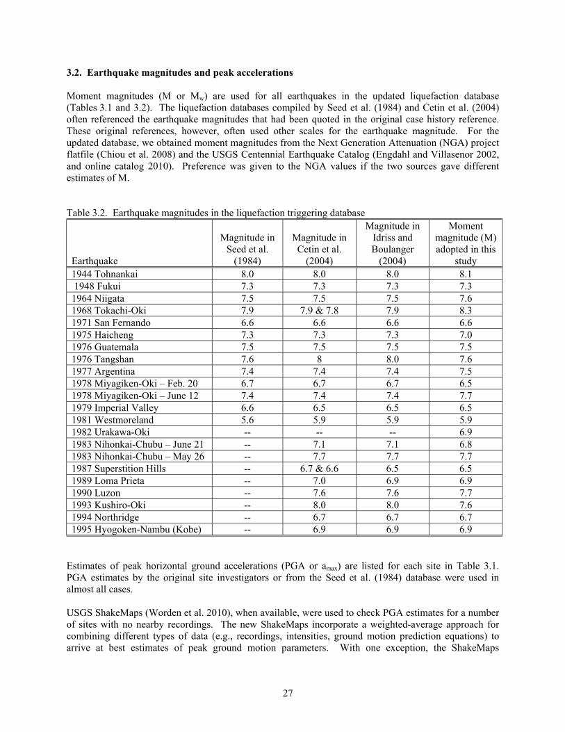
3.2. Earthquake magnitudes and peak accelerations Moment magnitudes (M or Mw) are used for all earthquakes in the updated liquefaction database (Tables 3.1 and 3.2). The liquefaction databases compiled by Seed et al. (1984) and Cetin et al. (2004) often referenced the earthquake magnitudes that had been quoted in the original case history reference. These original references, however, often used other scales for the earthquake magnitude. For the updated database, we obtained moment magnitudes from the Next Generation Attenuation (NGA) project flatfile (Chiou et al. 2008) and the USGS Centennial Earthquake Catalog (Engdahl and Villasenor 2002, and online catalog 2010). Preference was given to the NGA values if the two sources gave different estimates of M. Table 3.2. Earthquake magnitudes in the liquefaction triggering database Earthquake

Magnitude in

Seed et al. (1984)

Magnitude in

Cetin et al. (2004)

Magnitude in Idriss and Boulanger

(2004)

Moment magnitude (M) adopted in this

study 1944 Tohnankai 8.0 8.0 8.0 8.1 1948 Fukui 7.3 7.3 7.3 7.3 1964 Niigata 7.5 7.5 7.5 7.6 1968 Tokachi-Oki 7.9 7.9 & 7.8 7.9 8.3 1971 San Fernando 6.6 6.6 6.6 6.6 1975 Haicheng 7.3 7.3 7.3 7.0 1976 Guatemala 7.5 7.5 7.5 7.5 1976 Tangshan 7.6 8 8.0 7.6 1977 Argentina 7.4 7.4 7.4 7.5 1978 Miyagiken-Oki – Feb. 20 6.7 6.7 6.7 6.5 1978 Miyagiken-Oki – June 12 7.4 7.4 7.4 7.7 1979 Imperial Valley 6.6 6.5 6.5 6.5 1981 Westmoreland 5.6 5.9 5.9 5.9 1982 Urakawa-Oki -- -- -- 6.9 1983 Nihonkai-Chubu – June 21 -- 7.1 7.1 6.8 1983 Nihonkai-Chubu – May 26 -- 7.7 7.7 7.7 1987 Superstition Hills -- 6.7 & 6.6 6.5 6.5 1989 Loma Prieta -- 7.0 6.9 6.9 1990 Luzon -- 7.6 7.6 7.7 1993 Kushiro-Oki -- 8.0 8.0 7.6 1994 Northridge -- 6.7 6.7 6.7 1995 Hyogoken-Nambu (Kobe) -- 6.9 6.9 6.9

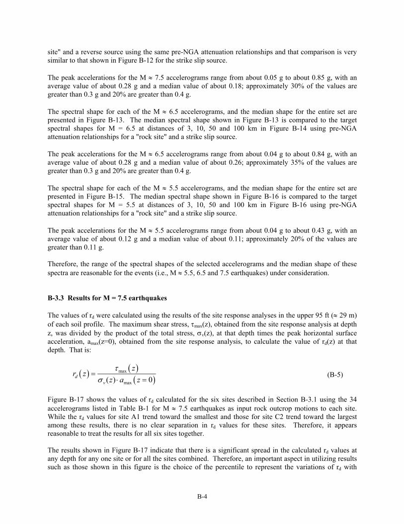
Estimates of peak horizontal ground accelerations (PGA or amax) are listed for each site in Table 3.1. PGA estimates by the original site investigators or from the Seed et al. (1984) database were used in almost all cases. USGS ShakeMaps (Worden et al. 2010), when available, were used to check PGA estimates for a number of sites with no nearby recordings. The new ShakeMaps incorporate a weighted-average approach for combining different types of data (e.g., recordings, intensities, ground motion prediction equations) to arrive at best estimates of peak ground motion parameters. With one exception, the ShakeMaps

28

confirmed that existing estimates of PGA were reasonable, such that no changes to these estimates were warranted. The ShakeMap for the 1975 Haicheng earthquake, however, indicated that significant changes to PGA estimates were warranted for some sites affected by the earthquake. The ShakeMap showing contours of PGA (in percentages) for the 1975 Haicheng earthquake is shown in Figure 3.1, along with the original reference's map of seismic intensities. Seed et al. (1984) had estimated values of PGA of 0.10, 0.13, 0.20, and 0.20 for the Shuang Tai Zi River Sluice Gate, Panjin Chemical Fertilizer Plant, Ying Kou Glass Fibre Plant, and Ying Kou Paper Plant, respectively, based on a correlation between seismic intensity and PGA. The USGS ShakeMap for this earthquake indicates best estimates of PGA would be at least 0.20, 0.20, 0.30, and 0.30 for these four sites, respectively.

(a) Contours of seismic intensity used by Shengcong and Tatsuoka (1984)

and Seed et al. (1984) to estimate PGA at case history sites

(b) Contours of PGA in percent from USGS ShakeMap (2010)

Figure 3.1. Ground motion estimates for the 1975 Haicheng earthquake

29

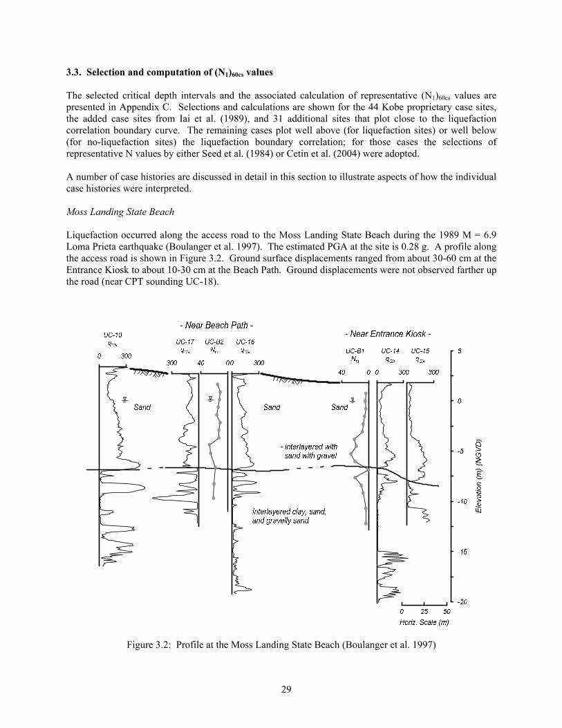
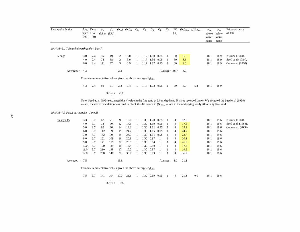
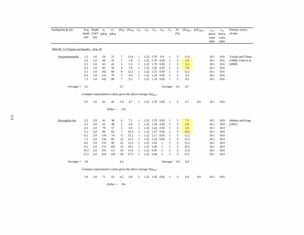
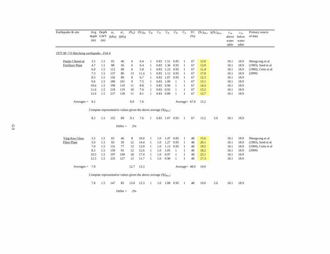
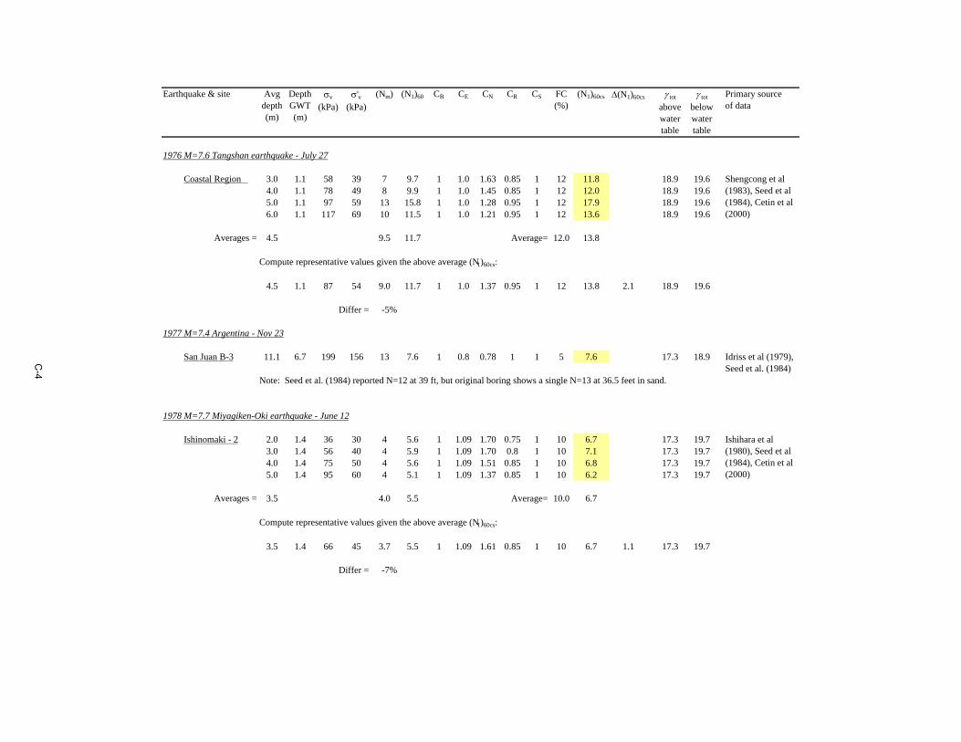
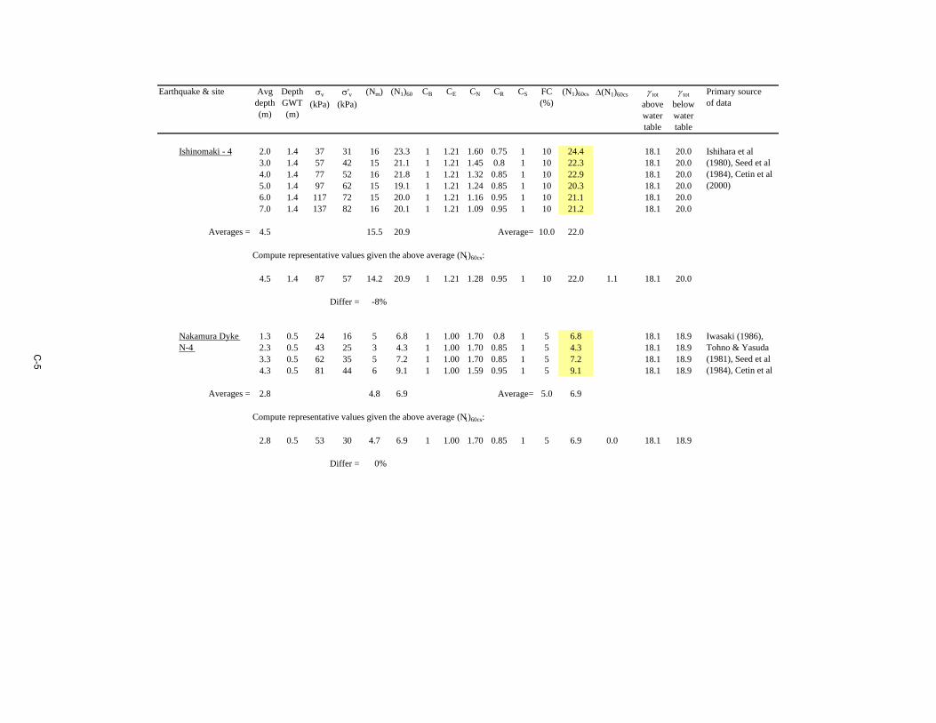
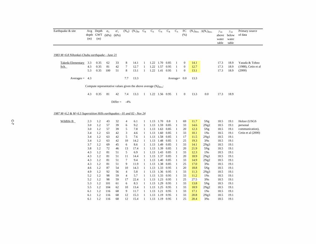
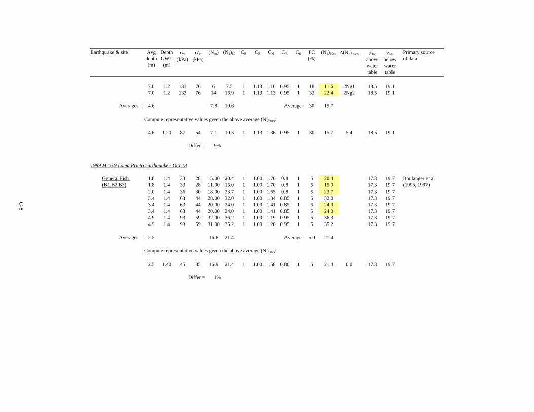
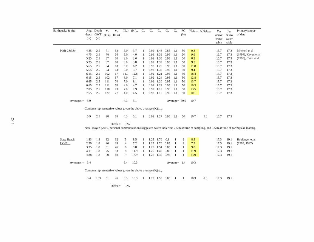
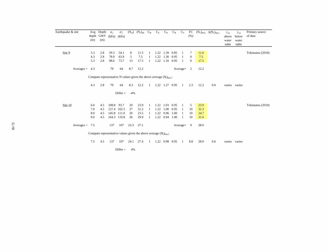
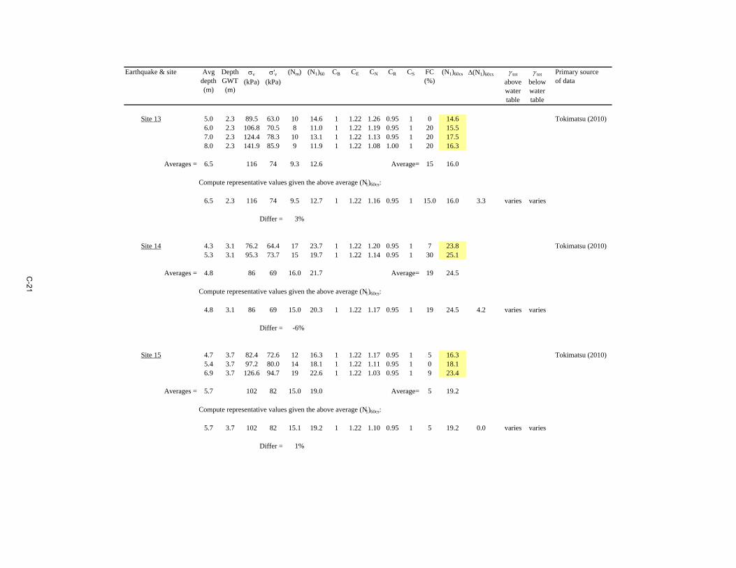
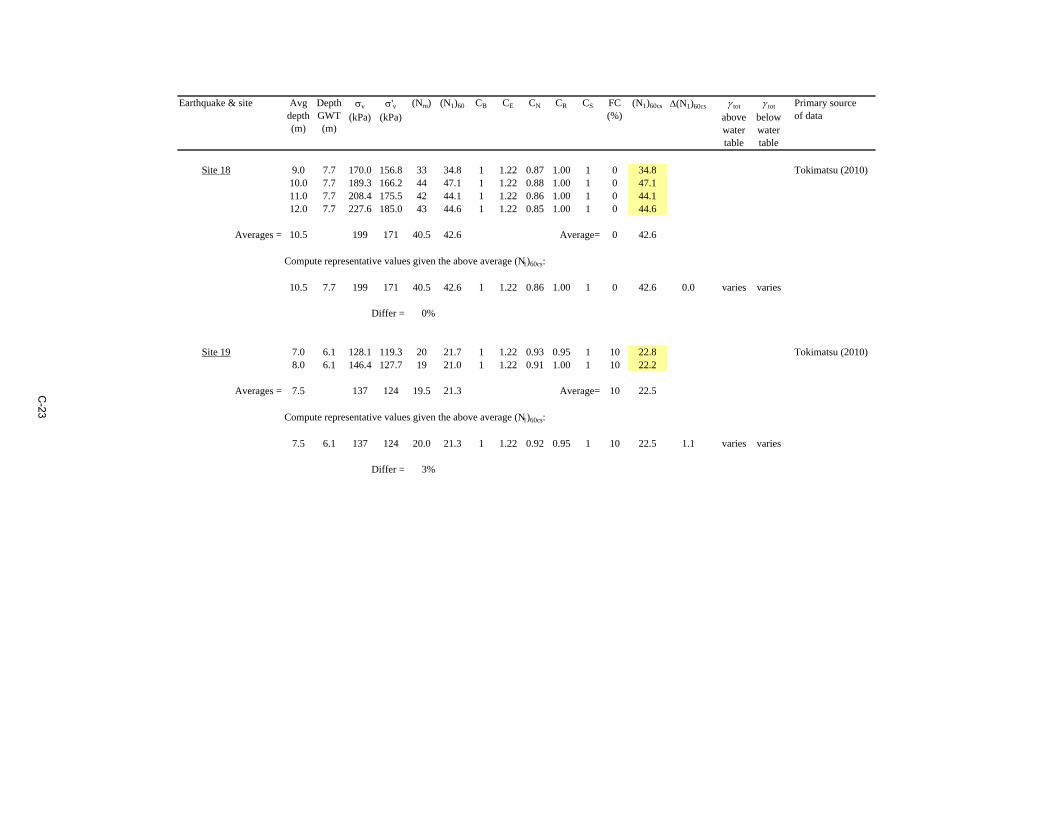
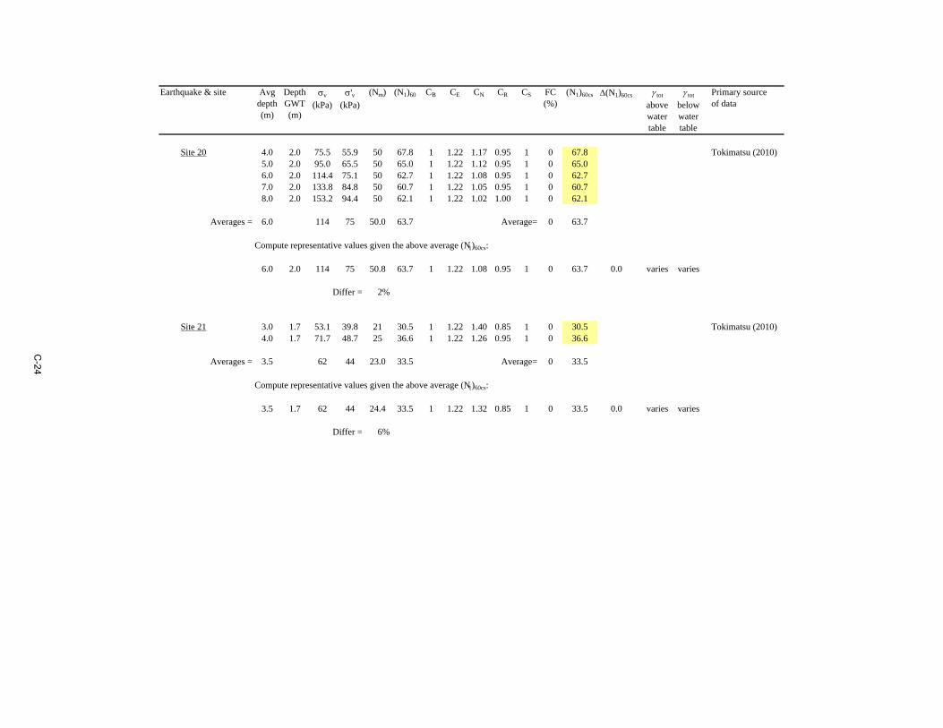
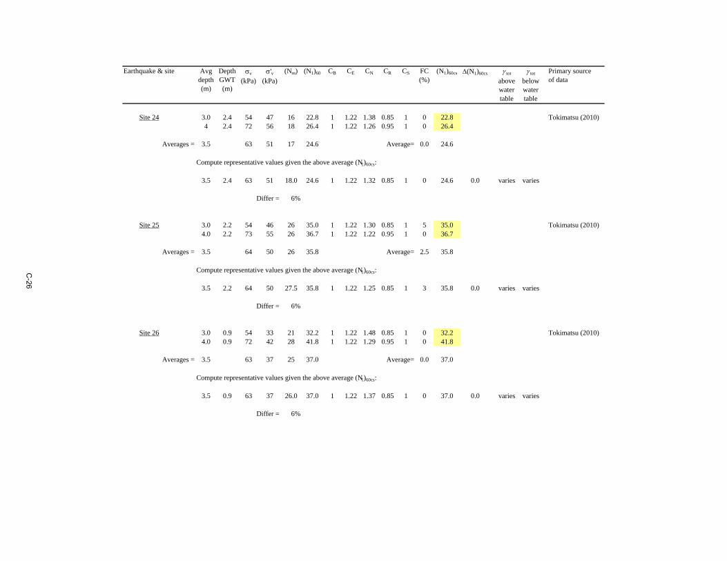
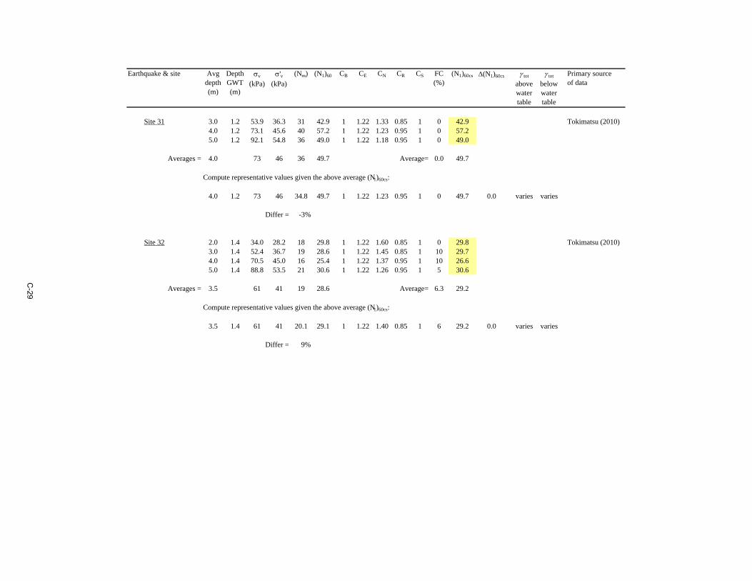
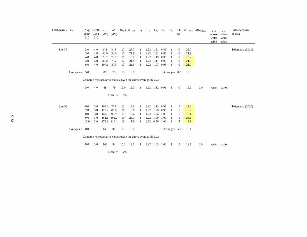
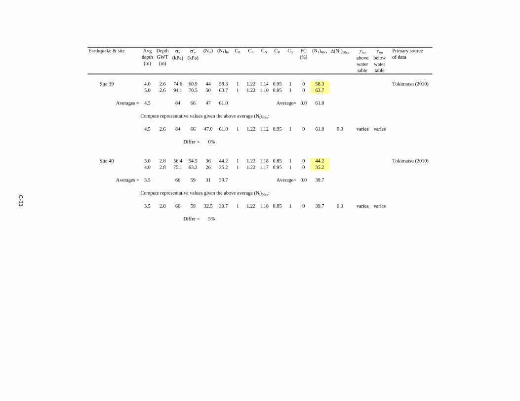
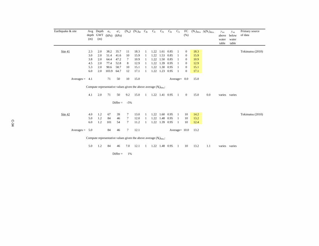
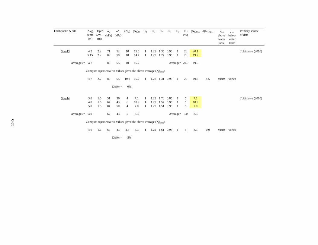
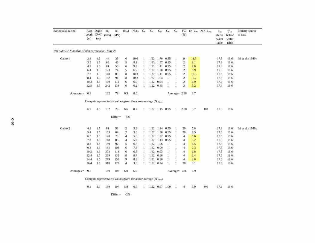
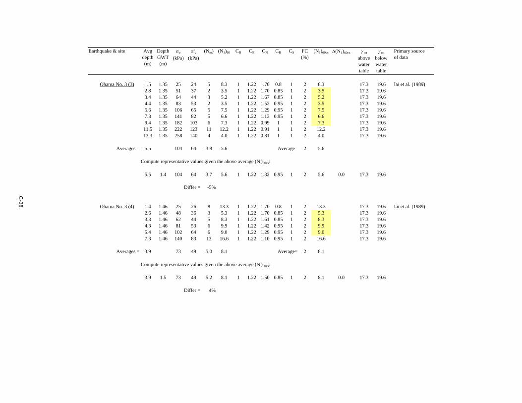
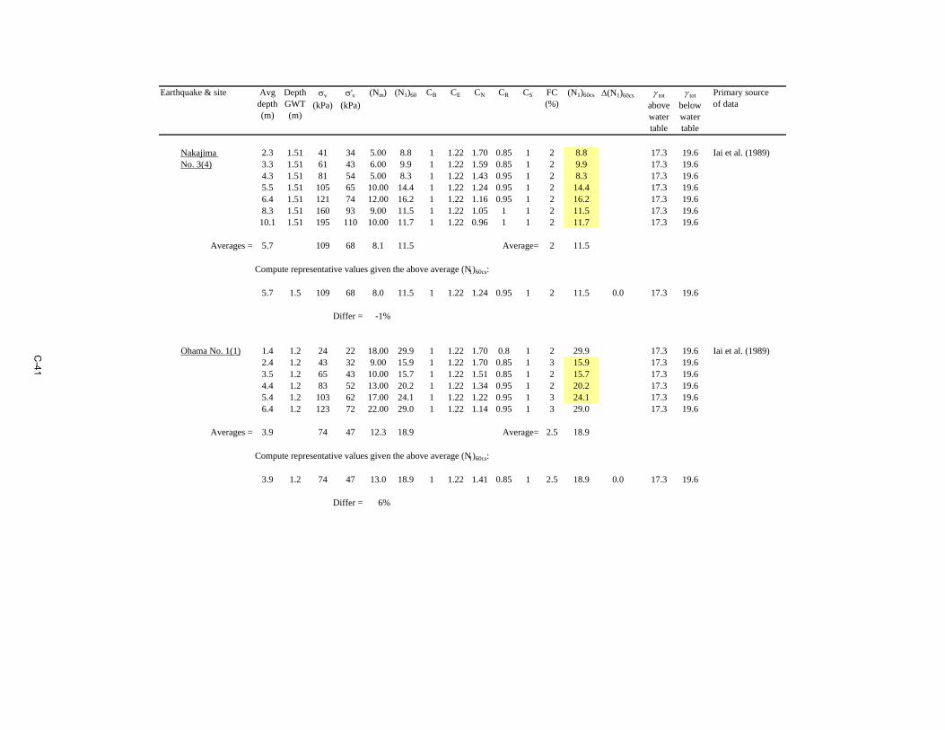
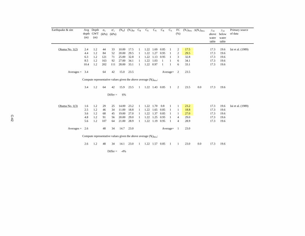
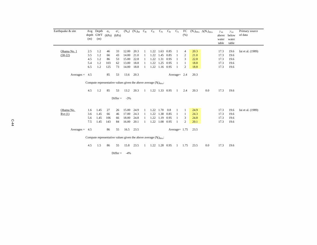
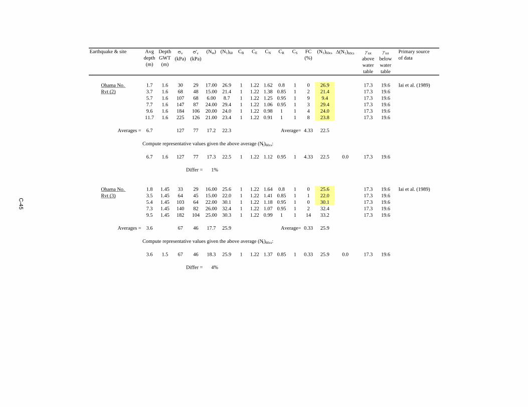
3.3. Selection and computation of (N1)60cs values The selected critical depth intervals and the associated calculation of representative (N1)60cs values are presented in Appendix C. Selections and calculations are shown for the 44 Kobe proprietary case sites, the added case sites from Iai et al. (1989), and 31 additional sites that plot close to the liquefaction correlation boundary curve. The remaining cases plot well above (for liquefaction sites) or well below (for no-liquefaction sites) the liquefaction boundary correlation; for those cases the selections of representative N values by either Seed et al. (1984) or Cetin et al. (2004) were adopted. A number of case histories are discussed in detail in this section to illustrate aspects of how the individual case histories were interpreted. Moss Landing State Beach Liquefaction occurred along the access road to the Moss Landing State Beach during the 1989 M = 6.9 Loma Prieta earthquake (Boulanger et al. 1997). The estimated PGA at the site is 0.28 g. A profile along the access road is shown in Figure 3.2. Ground surface displacements ranged from about 30-60 cm at the Entrance Kiosk to about 10-30 cm at the Beach Path. Ground displacements were not observed farther up the road (near CPT sounding UC-18).

Figure 3.2: Profile at the Moss Landing State Beach (Boulanger et al. 1997)

30

At the Beach Path, the first five measured SPT Nm values below the water table in boring UC-B2 were 14, 16, 11, 13, and 13, after which they increased to over 20. The computations of (N1)60cs values for the first five Nm values are summarized in Table 3.3. The average of the lower three (N1)60cs values is 16.9, whereas the average of the five (N1)60cs values is 18.4. The lateral spreading displacement of 10-30 cm would represent a shear strain of about 4-13% across a 2.3-m thick zone, or 3-8% across a 3.8-m-thick zone. While either of these average (N1)60cs values could be an acceptable choice for representing this site, the value of 18.4 was adopted as representative of this stratum. For forward evaluations, however, the choice of (N1)60cs = 16.9 would be more conservative. Table 3.3. Computation of the representative (N1)60cs value for UC-B2 at Moss Landing

The above table also illustrates a bookkeeping detail about reporting representative values for all the other parameters. The issue is that computing representative values for (N1)60 and (N1)60cs using the average values for depth, Nm, and FC, does not produce values equal to those obtained by directly averaging (N1)60 and (N1)60cs. Alternatively, the representative value of Nm can be back-calculated based on the average values for depth and FC along with the averaged values of (N1)60 and (N1)60cs. In the above table, the back-calculated representative Nm value is 12.8, which is only 5% less than the average Nm of 13.4. This difference can be positive or negative, but is almost always less than a few percent (see Appendix C). The advantage of the latter approach (bottom row in the above table) is that the reported values are internally consistent, which has its advantage for others who wish to use the database for sensitivity analyses. At the Entrance Kiosk, the first five Nm values below the water table in boring UC-B1 were 5, 4, 6, 8, and 9, after which they increased markedly. The first three N values represent a 2-m thick interval of the upper clean sand strata, for which the average of the corresponding three (N1)60cs values is 8.5. If the first five N values, representing a 3.5-m thick interval, are assumed to have liquefied, then the average (N1)60cs value is 10.3. The value of 10.3 was adopted as representative of this stratum for this case history. For forward evaluations, however, the choice of (N1)60cs = 8.5 would be more conservative. Consider the forward analysis of these two sites based on this method for selecting representative (N1)60cs values. If there was an earthquake that was just strong enough to produce a computed FSliq = 1.0 for the representative (N1)60cs value of 18.4 at the Beach Path, then the FSliq would be less than 1.0 for three of the five SPT tests in the looser strata. Since ground deformations may develop over thinner intervals within the identified strata, this approach for selecting representative (N1)60cs values should result in the liquefaction correlation (which generally bounds the bulk of the data) being conservative for forward applications in practice. In fact, in many instances it may prove most effective to treat each blow count separately in forward applications, rather than using an average value. In other instances, such as

Depth (m) Depth to

GWT (m)

vc

(kPa)

'vc (kPa)

(Nm) (N1)60 CB CE CN CR CS FC

(%)

(N1)60,cs (N1)60,cs

3.4 2.6 60 52 14 19.9 1 1.25 1.34 0.85 1 1 19.9

4.1 2.6 75 60 16 21.3 1 1.25 1.25 0.85 1 1 21.3

4.9 2.6 90 67 11 15.9 1 1.25 1.22 0.95 1 1 15.9

5.6 2.6 105 75 13 17.8 1 1.25 1.15 0.95 1 1 17.8

6.4 2.6 120 82 13 17.0 1 1.25 1.10 0.95 1 1 17.0

Average values:

4.9 13.4 18.4 1 18.4

Representative values given the above averages:

4.9 2.60 90 67 12.8 18.4 1 1.25 1.20 0.95 1 1 18.4 0.0

31

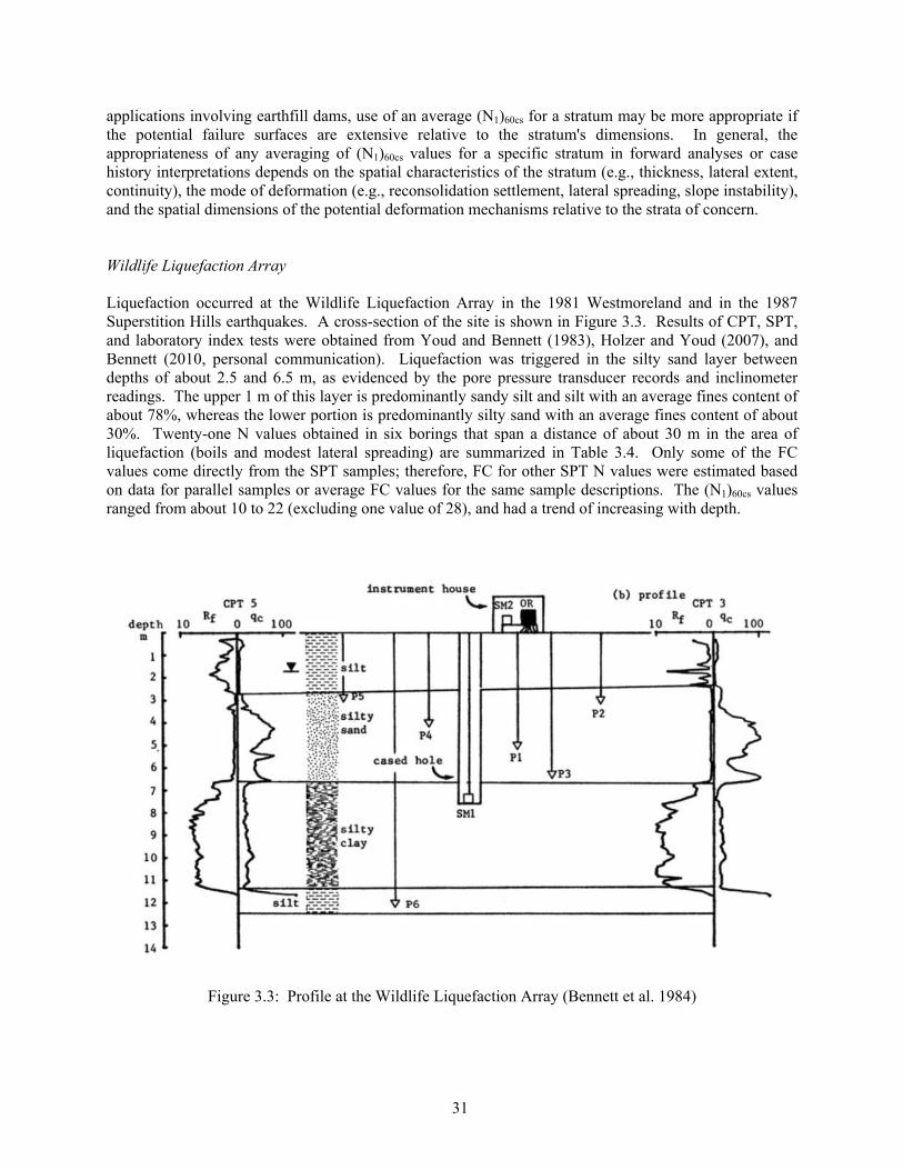
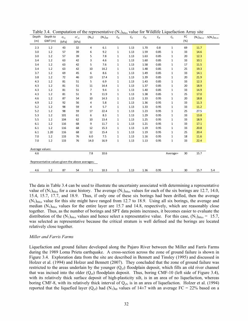
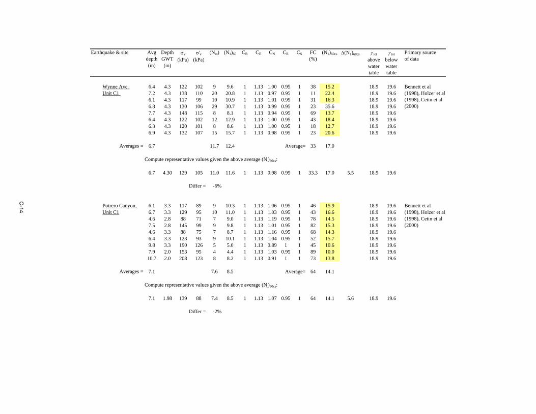
applications involving earthfill dams, use of an average (N1)60cs for a stratum may be more appropriate if the potential failure surfaces are extensive relative to the stratum's dimensions. In general, the appropriateness of any averaging of (N1)60cs values for a specific stratum in forward analyses or case history interpretations depends on the spatial characteristics of the stratum (e.g., thickness, lateral extent, continuity), the mode of deformation (e.g., reconsolidation settlement, lateral spreading, slope instability), and the spatial dimensions of the potential deformation mechanisms relative to the strata of concern. Wildlife Liquefaction Array Liquefaction occurred at the Wildlife Liquefaction Array in the 1981 Westmoreland and in the 1987 Superstition Hills earthquakes. A cross-section of the site is shown in Figure 3.3. Results of CPT, SPT, and laboratory index tests were obtained from Youd and Bennett (1983), Holzer and Youd (2007), and Bennett (2010, personal communication). Liquefaction was triggered in the silty sand layer between depths of about 2.5 and 6.5 m, as evidenced by the pore pressure transducer records and inclinometer readings. The upper 1 m of this layer is predominantly sandy silt and silt with an average fines content of about 78%, whereas the lower portion is predominantly silty sand with an average fines content of about 30%. Twenty-one N values obtained in six borings that span a distance of about 30 m in the area of liquefaction (boils and modest lateral spreading) are summarized in Table 3.4. Only some of the FC values come directly from the SPT samples; therefore, FC for other SPT N values were estimated based on data for parallel samples or average FC values for the same sample descriptions. The (N1)60cs values ranged from about 10 to 22 (excluding one value of 28), and had a trend of increasing with depth.

Figure 3.3: Profile at the Wildlife Liquefaction Array (Bennett et al. 1984)

32

Table 3.4. Computation of the representative (N1)60cs value for Wildlife Liquefaction Array site

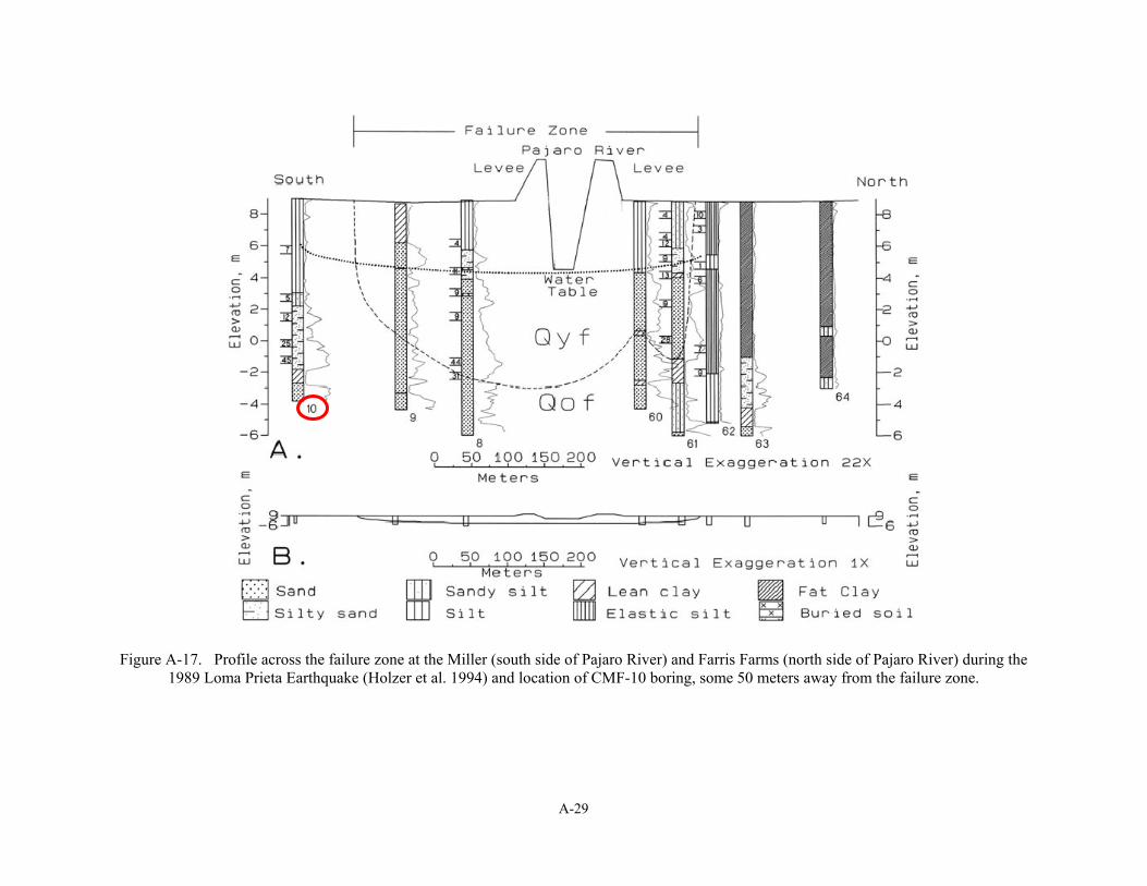
The data in Table 3.4 can be used to illustrate the uncertainty associated with determining a representative value of (N1)60cs for a case history. The average (N1)60cs values for each of the six borings are 12.7, 14.0, 15.4, 15.7, 17.7, and 18.9. Thus, if only one of these six borings had been drilled, then the average (N1)60cs value for this site might have ranged from 12.7 to 18.9. Using all six borings, the average and median (N1)60cs values for the entire layer are 15.7 and 14.8, respectively, which are reasonably close together. Thus, as the number of borings and SPT data points increases, it becomes easier to evaluate the distribution of the (N1)60cs values and hence select a representative value. For this case, (N1)60cs = 15.7, was selected as representative because the critical stratum is well defined and the borings are located relatively close together. Miller and Farris Farms Liquefaction and ground failure developed along the Pajaro River between the Miller and Farris Farms during the 1989 Loma Prieta earthquake. A cross-section across the zone of ground failure is shown in Figure 3.4. Exploration data from the site are described in Bennett and Tinsley (1995) and discussed in Holzer et al. (1994) and Holzer and Bennett (2007). They concluded that the zone of ground failure was restricted to the areas underlain by the younger (Qyf) floodplain deposit, which fills an old river channel that was incised into the older (Qof) floodplain deposit. Thus, boring CMF-10 (left side of Figure 3.4), with its relatively thick surface deposit of high-plasticity silt, is in an area of no liquefaction, whereas boring CMF-8, with its relatively thick interval of Qyf, is in an area of liquefaction. Holzer et al. (1994) reported that the liquefied layer (Qyf) had (N1)60 values of 14±7 with an average FC = 22% based on a

Depth

(m)

Depth to

GWT (m)vc

(kPa)

'vc (kPa)

(Nm) (N1)60 CB CE CN CR CS FC

(%)(N1)60,cs (N1)60,cs

2.3 1.2 43 32 4 6.1 1 1.13 1.70 0.8 1 69 11.7

3.0 1.2 57 39 6 9.2 1 1.13 1.59 0.85 1 33 14.6

3.0 1.2 57 39 5 7.8 1 1.13 1.63 0.85 1 20 12.3

3.4 1.2 63 42 3 4.6 1 1.13 1.60 0.85 1 33 10.1

3.4 1.2 63 42 5 7.6 1 1.13 1.58 0.85 1 17 11.5

3.4 1.2 63 42 10 14.2 1 1.13 1.48 0.85 1 25 19.3

3.7 1.2 69 45 6 8.6 1 1.13 1.49 0.85 1 33 14.1

3.8 1.2 72 46 13 17.4 1 1.13 1.39 0.85 1 20 21.9

4.3 1.2 81 51 5 6.9 1 1.13 1.43 0.85 1 33 12.3

4.3 1.2 81 51 11 14.4 1 1.13 1.37 0.85 1 20 18.9

4.3 1.2 81 51 7 9.4 1 1.13 1.40 0.85 1 33 14.9

4.3 1.2 81 51 9 11.9 1 1.13 1.38 0.85 1 25 17.0

4.6 1.2 87 54 10 14.3 1 1.13 1.33 0.95 1 20 18.8

4.9 1.2 92 56 4 5.8 1 1.13 1.36 0.95 1 33 11.3

5.2 1.2 98 59 4 5.7 1 1.13 1.33 0.95 1 33 11.2

5.2 1.2 98 59 17 22.4 1 1.13 1.23 0.95 1 25 27.5

5.3 1.2 101 61 6 8.3 1 1.13 1.29 0.95 1 33 13.8

5.5 1.2 104 62 10 13.4 1 1.13 1.25 0.95 1 33 18.9

6.1 1.2 116 68 9 11.7 1 1.13 1.21 0.95 1 33 17.1

6.1 1.2 116 68 12 15.3 1 1.13 1.19 0.95 1 33 20.8

6.1 1.20 116 68 12 15.4 1 1.13 1.19 0.95 1 25 20.4

7.0 1.2 133 76 6.0 7.5 1 1.13 1.16 0.95 1 18 11.6

7.0 1.2 133 76 14.0 16.9 1 1.13 1.13 0.95 1 33 22.4

Average values:

4.6 7.8 10.6 Average= 30 15.7

Representative values given the above averages:

4.6 1.2 87 54 7.1 10.3 1 1.13 1.36 0.95 1 30 15.7 5.4

33

total of 15 blow counts from several borings. The variation in average (N1)60 values for the liquefied layer from individual borings is illustrated by considering borings CMF-3, -5, and -8 which spanned a distance of about 550 m within the failure zone parallel to the river; these borings had 3, 1, and 3 blow counts in the liquefied layer, respectively, from which representative (N1)60 values of 9.9, 20.9, and 9.8 with FC of 27%, 13%, and 25% were obtained, respectively. Some of the variability in these average (N1)60 values is likely due to the small sample sizes (i.e., one to three blow counts cannot be expected to provide an accurate indication of the true average blow count in the vicinity of a boring), while some of it could be due to systematic variations in the average (N1)60 value across the site. These three borings are listed separately in Table 3.4 because of the relatively large distances between any two borings. For the nonliquefied layer (Qof), a representative (N1)60 value of 20.2 for boring CMF-10 was obtained by averaging the two lower blow counts (12 and 25) with FC = 20%, which resulted in a representative (N1)60cs = 24.6. This site is one of several examples used by Holzer and Bennett (2007) to illustrate how the boundaries of a lateral spread are often controlled by changes in geologic facies. It also illustrates how borings located short distances outside of a ground failure zone may, or may not, be representative of the soils that have liquefied. For this reason, the interpretation of liquefaction case histories using borings located outside the failure zone have the potential to be misinterpreted unless the geologic conditions are fully understood and taken into consideration. It also emphasizes the need for investigators to incorporate and include the geologic conditions in the description of the case histories investigated.

Figure 3.4. Profile across the failure zone at the Miller (south side of Pajaro River) and Farris Farms (north side of Pajaro River) during the 1989 Loma Prieta Earthquake (Holzer et al. 1994)

34

Balboa Boulevard Liquefaction and ground failure developed along Balboa Boulevard during the 1994 Northridge earthquake. The estimated PGA at the site was about 0.84 g (Holzer et al. 1999). A cross-section across the zone of ground failure is shown in Figure 3.5. Exploration data from the site and interpretations of the behavior are presented by Holzer et al. (1999) and discussed by O'Rourke (1998). The site is underlain by an 8- to 10-m-thick stratum of Holocene silty sand and lean clay with sand; the upper 1-m-thick unit is fill (Unit A), underlain by sheet flood and debris flow deposits (Unit B), and then fluvial deposits (Unit C). These Holocene deposits are underlain by Pleistocene silty sand (Unit D), which was identified as the Saugus formation. Holzer et al. (1999) calculated average (N1)60cs values for Units C and D using the procedures described in Youd et al. (2001), which had been initially published in an NCEER report in 1997 (NCEER 1997). For Unit C, 8 SPT blow counts were obtained, of which 4 were in clayey sands and 4 were in silty sands; the average of the 4 tests in silty sands gave an (N1)60cs value of 21 with FC = 42%. For Unit D, 44 SPT N values were obtained, of which 15 were in clayey sands and 29 were in silty sands; the average of the 29 tests in silty sands gave an (N1)60cs value of 59 with FC = 36%. Permanent ground deformations were limited to the area where the water table is within the Holocene sediments, such that the silty sand soils within Unit C were identified as the material that liquefied during the earthquake. The procedures described in this report produce a representative (N1)60cs value of 18.7 for Unit C based on the average of the 4 SPT blow counts obtained in the silty sands of this stratum, as outlined in Appendix C. Holzer et al. (1999) and Holzer and Bennett (2007) noted that the Balboa Boulevard site is an example of how the location of lateral spreading and ground failure can be controlled by the position of the ground water table relative to the geologic strata. As shown in Figure 3.5, ground failure along Balboa Boulevard was limited to the area where the ground water table was within the Holocene sediments, while no ground failure was observed where the ground water table was within the underlying, denser Pleistocene sediments. This case history also illustrates how the identification of the major geologic facies can be essential for understanding or predicting the extent and location of ground failure during earthquakes.

35

Figure 3.5: Profile across the failure zone at the Balboa Boulevard site during the 1994 Northridge Earthquake (Holzer et al. 1999)

36

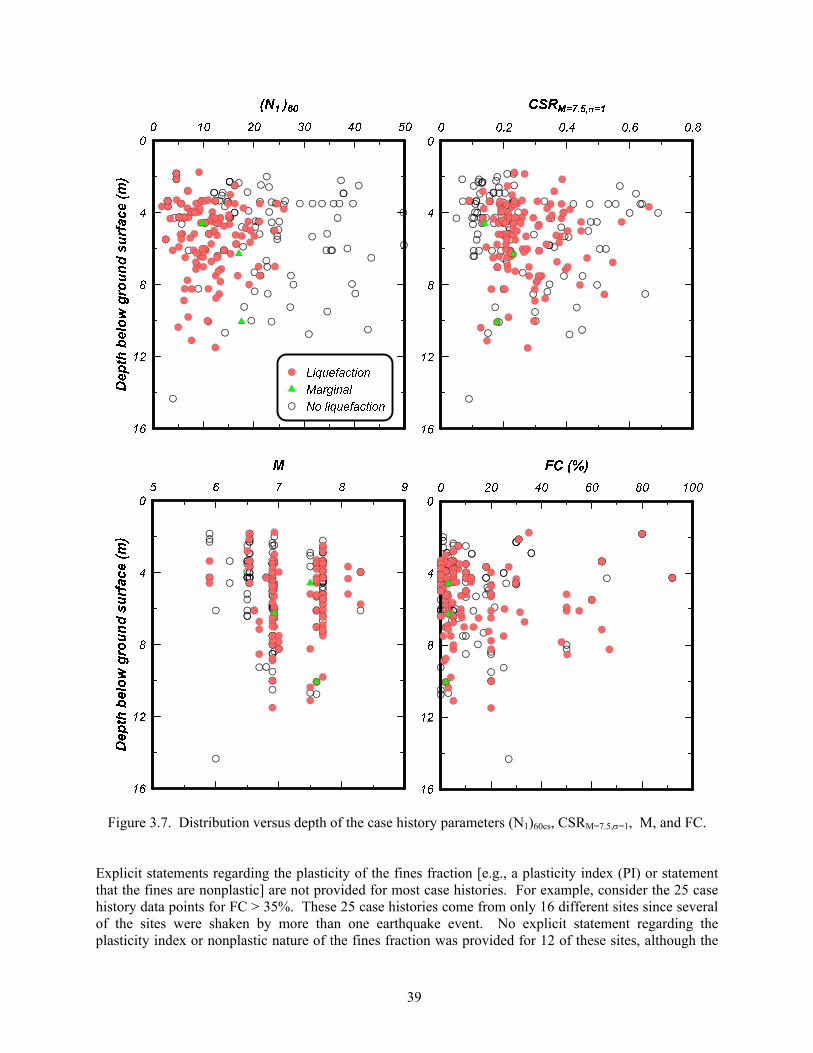
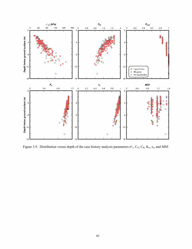
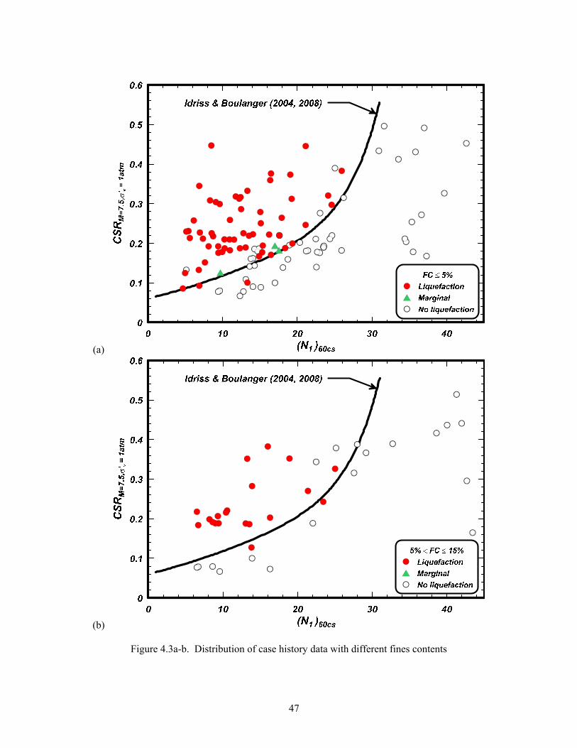
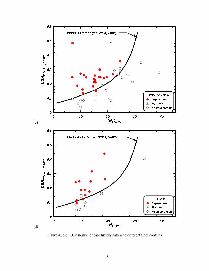
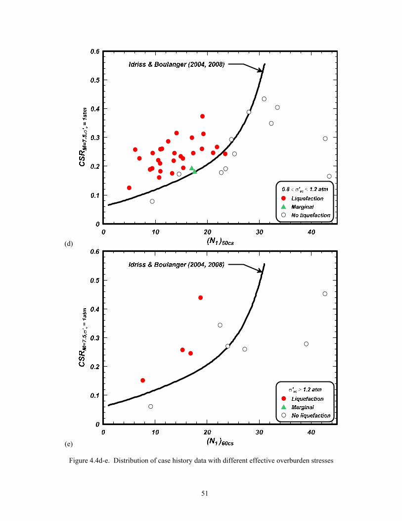
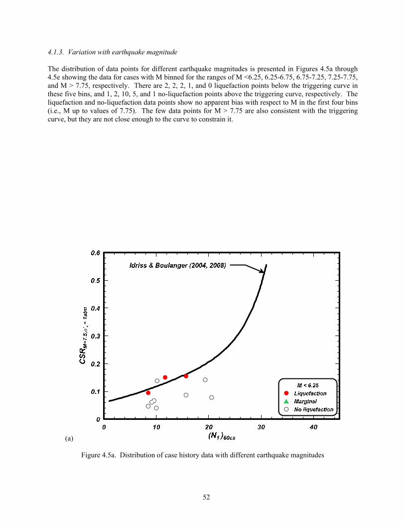
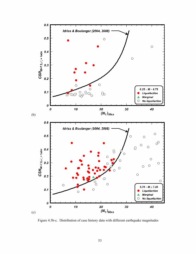
Malden Street Ground failure along Malden Street during the 1994 Northridge earthquake is an example of ground failure due to lurching in soft clays (O'Rourke 1998, Holzer et al. 1999). The estimated PGA at this location was 0.51 g. A cross-section across the ground failure zone is shown in Figure 3.6. The failure zone is underlain by an 8.5-m-thick stratum of Holocene lean to sandy lean clay (Units A and B), which is underlain by Pleistocene silty sand (Unit D). The ground water table in the failure zone was at a depth of 3.9 m, and no Holocene sands were encountered below the water table. The fine grained soils of Unit B typically had FC > 70% with an average PI of 18. Undrained shear strengths (su) for Units A and B were determined from field vane shear tests and CPT data. The su in Unit B was generally less than 50 kPa, compared to about 120 kPa for Unit A, and it decreased to an average value of su = 26 kPa in the 1.5-m-thick interval between depths 4.3 and 5.8 m in the area of ground failure. Holzer et al. (1999) computed peak dynamic shear stresses, based on the estimated PGA of 0.51 g that were about twice the soil's undrained shear strength. For the underlying Pleistocene sediment (Unit D), Holzer et al. (1999) obtained 8 SPT blow counts, of which 2 were in silty sands and 6 were in clayey sands; they reported an average (N1)60cs value of 43 (using the procedures from Youd et al. 2001) with an average FC = 27% based on the two tests in silty sands. Holzer et al. (1999) and O'Rourke (1998) both concluded that cyclic softening/failure of the soft clay along Malden Street caused the observed ground deformations. In fact, O'Rourke used this site as a key example of ground failure due to lurching in soft clays, and not liquefaction of a cohesionless deposit. This case history illustrates the importance of recognizing that ground failures can develop in soft clays under strong earthquake shaking, which is important to the interpretation of ground failure case histories and to the forward prediction of ground failures in practice. Additional case histories from the 1999 Chi-Chi and Kocaeli earthquakes have provided several examples regarding the behavior of low-plasticity fine grained soils, including cases of ground failure attributed to cyclic softening of silty clays beneath strongly loaded foundations (e.g., Chu et al. 2008) and cases where the low but measurable plasticity of the fines fraction was identified as one of the characteristics associated with lateral spreading displacements being significantly smaller than would be predicted by the application of current liquefaction analysis procedures (e.g., Chu et al. 2006, Youd et al. 2009). 3.4. Classification of site performance Site performance during an earthquake is classified as a "liquefaction", "no liquefaction", or a "marginal" case; some databases designate these cases as "yes", "no", or "no/yes", respectively. In this report, the classification of site performance was based on the classification assigned by the original investigator, except for the Seventh Street Wharf site at the Port of Oakland (discussed below). Cases described as "liquefaction" were generally accompanied with reports of sand boils and/or visible ground surface settlements, cracks, or lateral spreading movements. Cases described as "no liquefaction" were either accompanied with reports of no visible surface manifestations (i.e., no sand boils, ground surface settlements, cracks, or lateral movements) or can be inferred as having corresponded to such conditions when not explicitly stated. A case is described as "marginal" if the available information suggests that conditions at the site are likely at, or very near, the boundary of conditions that separate the occurrence of liquefaction from nonliquefaction. Only three cases are classified as marginal in the database because it is very difficult to define a marginal case in most field conditions. Areas of liquefaction and nonliquefaction in the field are often separated by distinct geologic boundaries (e.g., Holzer and Bennett 2007) such that borehole data can be used to describe liquefaction and no liquefaction cases, but not the marginal condition. Thus

37

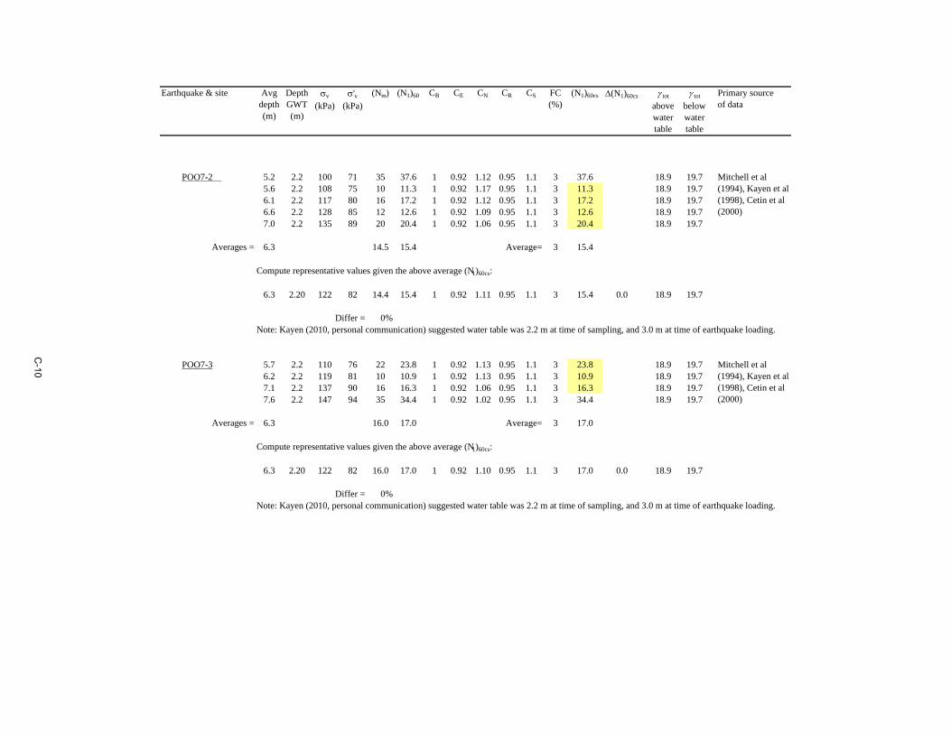
explicit information is typically not available for marginal conditions. The three marginal cases in the database are, therefore, discussed below. The Seventh Street Wharf site at the Port of Oakland and its performance in the 1989 Loma Prieta earthquake are described in Kayen et al. (1998) and Kayen and Mitchell (1998). Boring POO7-2 was intentionally located in an area with surface manifestations of liquefaction, whereas boring POO7-3 was in an area with no surface manifestations. The two borings, POO7-2 and POO7-3, were characterized as "liquefaction" and "no liquefaction" sites, respectively, in Kayen et al. (1998). The following additional information and updated interpretation of the performance of these sites was provided by Kayen (2010, personal communication). The two borings, POO7-2 and POO7-3, were separated by 70-100 m. At the location of POO7-3, there were no sand boils in the immediate 15-20 meters. This site was at the back of the park (now converted to container yard) at the farthest distance from the dike. In the zone along the bay margin, perhaps 20 m

Figure 3.6. Profile across the failure zone at the Malden Street site during the 1994 Northridge Earthquake (Holzer et al. 1999)

38

wide, there were ample fissures and sand boils, deformations toward the free-face, and a small lateral spread into the bay. The distance from this zone to POO7-3 was about 20-30 m. Kayen (2010, personal communication) indicated that, at this time, he would classify the location at POO7-3 as a liquefaction site because it was too close to the park perimeter deformations to be classified as a non-liquefaction site based on surface observations alone. This site was listed as a "marginal" case in the database presented herein because the soil conditions at POO7-3 had similar stratigraphy but slightly denser conditions than at POO7-2. Two other sites are listed as marginal cases in the database. Seed et al. listed the Rail Road 2 case as a "no/yes" case and assigned it a representative N value that corresponds to the value Koizumi (1966) considered to have been the critical value that separated cases of liquefaction from cases of no liquefaction in the Niigata earthquake. Thus, the N value assigned to the Rail Road 2 case was explicitly derived as a point that should fall on the triggering curve. The Amatitlan B-1, B-2, B-3, and B-4 cases from the 1976 Guatemala earthquake are described by Seed et al. (1979). Boring B-2 was intentionally located in a nonliquefied zone, but very close to the boundary between the areas of liquefaction and no-liquefaction. Seed et al. listed boring B-2 case as a "no/yes" case because they concluded that it probably represented the limiting conditions at which liquefaction would just occur or just not occur for the ground conditions and ground motions experienced at this site in the Guatemala earthquake. 3.5. Distribution of data The distributions of (N1)60, CSRM=7.5,=1, M, and FC from the database are plotted versus the average depths for the critical zones in Figure 3.7 for "liquefaction", "marginal", and "no liquefaction" cases. These figures indicate that the database is limited to average critical depths less than 12 m and has very few data points for M greater than 7.7 or less than 6.4 or for FC greater than 40%. The distributions of the data are further illustrated in Figure 3.8 showing amax versus M (two parameters which enter the calculation of CSRM=7.5,=1) and FC versus (N1)60 (two parameters which enter the calculation of (N1)60cs). The plot of FC versus (N1)60 indicates that the data points for FC greater than about 25% are largely limited to (N1)60 values less than about 15. The distributions of 'v, CN, CR, K, rd, and MSF are plotted versus average depth in Figure 3.9. The computed values for 'v are generally less than about 140 kPa, the CN factors are generally between 0.8 and 1.7 (cutoff value), the Kvalues are generally between 0.9 and 1.1 (cutoff value), and rd values are generally greater than 0.8. The maximum depth and average depth for the critical zones are compared in Figure 3.10; for example, if the critical zone for a site extended between depths of 6 m and 10 m, the average depth would be 8 m while the maximum depth would be 10 m. This figure includes all the cases (liquefaction or no liquefaction) for which a detailed calculation of the average (N1)60cs value was performed (Appendix C). This figure shows that there were a significant number of cases for which the critical zone extended to maximum depths of about 12 to 13 m, whereas Figures 3.7 and 3.9 indicate that there are relatively few cases for which the average depth of the critical zone was close to 12 m.

39

Explicit statements regarding the plasticity of the fines fraction [e.g., a plasticity index (PI) or statement that the fines are nonplastic] are not provided for most case histories. For example, consider the 25 case history data points for FC > 35%. These 25 case histories come from only 16 different sites since several of the sites were shaken by more than one earthquake event. No explicit statement regarding the plasticity index or nonplastic nature of the fines fraction was provided for 12 of these sites, although the

Figure 3.7. Distribution versus depth of the case history parameters (N1)60cs, CSRM=7.5,=1, M, and FC.

40

visual descriptions and classifications of the soils (e.g., SM, ML) implied either nonplastic or low-plasticity fines. For the critical layers at Van Norman and Juvenile Hall, Cetin et al. (2000) suggest PI values of 3-10 were representative of the fines fraction. For Unit C1 at Potrero Canyon (Bennett et al. 1998), the data from the SPT samples used to represent the liquefiable lenses (Appendix C) indicate an average FC = 64%, classifications as SM or ML, and PI values of 2-3 for three of the 9 samples (PI values not reported for the other samples); note that the summary in Holzer et al. (1999) suggests an average PI = 5 for the range of silt and silty sand in the C1 unit. For the saturated portion of Unit C at Balboa Boulevard (Bennett et al. 1998), the data from the four SPT samples in the sandy silt and silty sand portions of this stratum indicated an average FC = 50%, classifications as SM or ML, and no indication of plasticity; note that the summary in Holzer et al. (1999) suggests an average PI = 11 for the heterogeneous range of clays to silty sands in this stratum. While explicit information of fines plasticity is lacking throughout the case history database, it is believed that the database presented herein corresponds primarily to soils with essentially nonplastic or very low plasticity fines.

Figure 3.8. Distributions of amax versus M and FC versus (N1)60. Note that it appears that there are fewer

data points in the graph of amax versus M because many of the points plot on top of each other.

41

Figure 3.9. Distribution versus depth of the case history analysis parameters 'v, CN, CR, K, rd, and MSF.

42

Figure 3.10. Maximum depth for the critical zone versus the average depth for the critical zone.

43

4. EXAMINATION OF THE LIQUEFACTION TRIGGERING CORRELATION 4.1. Case history data This section contains an examination of the updated case history data, as described in Section 3 and listed in Table 3.1, for evidence of trends or biases relative to the liquefaction triggering correlation by Idriss and Boulanger (2004, 2008). The full, updated database is shown with the Idriss-Boulanger triggering correlation in terms of equivalent CSRM=7.5,'=1 versus equivalent clean sand (N1)60cs in Figure 4.1. For comparison, the database previously used by Idriss and Boulanger (2004, 2008) is shown in Figure 4.2. Comparison of Figure 4.1 with Figure 4.2 indicates that the updated database includes considerably more case histories and that the updated database continues to support the previously derived triggering correlation. The uncertainties in the measured or estimated (N1)60cs and CSRM=7.5,'v=1 values for each case history should be considered when evaluating the preferred position of a liquefaction triggering correlation relative to the case history data points. Specifically, the consequence of these measurement (or parameter) uncertainties is that a reasonably conservative, deterministic liquefaction triggering curve should not be expected to fully envelop all of the liquefaction case histories. Heuristically, a deterministic liquefaction triggering curve can be expected to be positioned so that the number of liquefaction case histories falling below the curve is relatively small compared to the number of no-liquefaction case histories falling above the curve. More formally, statistical methods can be used to address the influence of measurement uncertainties and evaluate the uncertainty in liquefaction triggering correlations. In this regard, the probabilistic analyses of the case history database presented in Section 6 of this report indicates that the deterministic liquefaction triggering curve by Idriss and Boulanger (2004, 2008) corresponds to a probability of liquefaction of about 16% based on model uncertainty alone [i.e., if the (N1)60cs and CSRM=7.5,'v=1 values are known perfectly] and to a probability of liquefaction of about 35% with the inclusion of measurement uncertainties [i.e., allowing for the uncertainty in the (N1)60cs and CSRM=7.5,'v=1 values for each case history]. Examination of the updated case history data (Table 3.1) included sorting the data into various parameter bins (e.g., soil characteristics, earthquake magnitudes, data sources, and individual earthquakes) and comparing the binned data to the Idriss-Boulanger triggering correlation. These comparisons are presented in terms of (N1)60cs so that the entire data (clean sands, silty sands and nonplastic sandy silts) can be combined in different data bins.

44

Figure 4.1. Updated SPT case history database of liquefaction in cohesionless soils with various fines contents in terms of equivalent CSR for M = 7.5 and 'v = 1 atm and equivalent clean sand (N1)60cs

Figure 4.2. SPT case history database used previously by Idriss and Boulanger (2004, 2008)

45

4.1.1. Variation with fines content The data for clean sands (FC ≤ 5%) are shown in the plot of CSRM=7.5,'v=1 versus (N1)60cs in Figure 4.3a. There are 2 liquefaction points that are below the Idriss-Boulanger triggering correlation and 8 no-liquefaction points above it. The Nakamura Dyke N-4 site in the February 20, 1978 Miyagiken-Oki earthquake is one of the liquefaction points with FC ≤ 5% that plots below the triggering curve. This case had a PGA = 0.12 g, a critical depth = 2.8 m, 'v = 30 kPa, (N1)60 = 6.9, and FC = 5%. The representative (N1)60cs value of 6.9 is based on the average of 4 N values (5, 3, 5, and 6) from a single boring. The Takeda Elementary School site in the June 21st aftershock of the 1983 Nihonkai-Chubu earthquake is the other liquefaction point with FC ≤ 5% that plots below the triggering curve. This case had an estimated PGA = 0.11 g, critical depth = 4.3 m, 'v = 42 kPa, (N1)60 = 13.3, and FC = 0%. The representative (N1)60cs value of 13.3 is based on the average of 3 N values (8, 7, & 8) from a single boring provided by the Nakazato Town Office to Yasuda and Tohno (1988). Yasuda and Tohno (1988) reported that this site liquefied during both the May 26th main shock and the June 21st aftershock (26 days later); they estimated the PGA as being 0.283 g and 0.111 g during the main shock and aftershock, respectively, based on recordings at a station 6 km away. The data for sands with 5% ≤ FC ≤ 15% are shown in the plot of CSRM=7.5,=1 versus (N1)60cs in Figure 4.3b. There are 2 liquefaction points that are below the Idriss-Boulanger triggering correlation and 2 no-liquefaction points above it. The Coastal region site in the 1976 Tangshan earthquake is one of the liquefaction points with 5% ≤ FC ≤ 15% that plots below the triggering curve. This case had PGA = 0.13 g, critical depth = 4.5 m, 'v = 54 kPa, (N1)60 = 11.7, and FC = 12%. The representative (N1)60cs value of 13.8 is based on the average of 4 N values (7, 8, 13, and 10) from a single boring. Had only the first two N values been used, then the resulting data point would be (N1)60cs = 9.7, which would be positioned just to the left (i.e. above) the triggering curve. The Miller Farm CMF-5 site in the 1989 Loma Prieta earthquake is the second liquefaction point with 5% ≤ FC ≤ 15% that plots below the triggering curve. This case corresponds to one of several borings within an area of liquefaction parallel to a river, as discussed in more detail in Section 3.3. The data for CMF-5 was PGA = 0.39 g, critical depth = 7.0 m, 'v = 108 kPa, (N1)60 = 20.9, and FC = 13%. The representative (N1)60cs value of 23.4 is based on a single N value from this boring. Two other borings within the failure zone, CMF-3 and CMF-8, each had three N values in the liquefied layer and had representative (N1)60cs values of 15.3 and 14.9, respectively. If an average (N1)60cs value had been adopted for the entire failure zone (i.e., averaging the data across these borings), the resulting data points would plot above the triggering curve. The data for these three borings were, however, plotted separately because they span a relatively large distance (about 550 m), and thus they may reflect spatial variability as well as the effect of small sample sizes. The data with 15% ≤ FC ≤ 35% are shown in Figure 4.3c. Two liquefaction data points, corresponding to the same site in two different earthquakes, fall just below the triggering curve and 4 no-liquefaction points are above it.

46

The Wildlife B site in the 1981 M = 5.9 Westmoreland and 1987 M = 6.5 Superstition Hills earthquakes represents the two data points with 15% ≤ FC ≤ 35% that plot below the triggering curve. This site was well characterized with 21 SPT N values from six borings, as described previously in Section 3.3. The data with FC ≥ 35% are shown in Figure 4.3d. There is 1 liquefaction data point that is just below the triggering curve and 3 no-liquefaction points that are above it. The Radio Tower B-1 site in the 1981 Westmoreland earthquake is the one liquefaction case with FC ≥ 35% that plots just below the triggering curve. This case had a PGA = 0.20 g, critical depth = 3.3 m, 'v = 49 kPa, (N1)60 = 2.9, and FC = 75%. The representative (N1)60cs value of 8.4 is based on a single N value from a single boring. The full dataset, including all fines contents, has a total of 7 points that fall below the triggering curve and 18 nonliquefaction points that are above it. The 3 marginal data points fall very close to, or slightly above, the triggering curve. The 7 points that fall below the triggering curve for the liquefaction cases are listed below: Table 4.1. Aspects of the seven data points falling below the Idriss-Boulanger triggering curve

Case (N1)60cs FC (%) CSRM=7.5,'v=1 atm* CRRM=7.5,'v=1 atm**

Increment below

triggering curve

Nakamura Dyke N-4 site (1978 M = 6.4 Miyagiken-Oki earthquake)

6.9 5 0.093 0.097 0.004

Takeda Elementary School site (June 21st M = 6.8 aftershock, 1983 Nihonkai-Chubu earthquake

13.3 0 0.101 0.142 0.041

Coastal region site (1976 M = 7.6 Tangshan earthquake)

13.8 12 0.127 0.146 0.019

Miller Farm CMF-5 site (1989 M = 6.9 Loma Prieta earthquake)

23.4 13 0.243 0.257 0.014

Wildlife B site (1981 M = 5.9 Westmoreland earthquake)

15.7 30 0.155 0.162 0.007

Wildlife B site (1987 M = 6.5 Superstition Hills earthquake)

15.7 30 0.148 0.162 0.014

Radio Tower B-1 site (1981 M = 5.9 Westmoreland earthquake)

8.4 75 0.094 0.107 0.013

* Value of CSRM=7.5,'v=1 atm for the case history. ** Value of CRRM=7.5,'v=1 atm from the triggering curve at (N1)60cs for the case history.

Except for the Takeda Elementary School site, these are minor differeces and do not warrant changing the triggering curve. Obviously, the liquefaction triggering correlation should not be controlled by a single case history, particularly given the potential effects of measurement uncertainties in the case history database. Therefore, the position of the triggering curve appears to be relatively unbiased with respect to fines content, and to be reasonably conservatively positioned.

47

(a)

(b)

Figure 4.3a-b. Distribution of case history data with different fines contents

48

(c)

(d)

Figure 4.3c-d. Distribution of case history data with different fines contents

49

4.1.2. Variation with effective overburden stress The distribution of data points for different vertical effective stresses is presented in Figures 4.4a through 4.4e showing the data for cases with 'v binned between 0-0.4 atm, 0.4-0.6 atm, 0.6-0.8 atm, 0.8-1.2 atm, and >1.2 atm, respectively. There are 1, 5, 0, 1, and 0 liquefaction points below the triggering curve in these five bins, respectively, and there are 4, 6, 5, 2, and 1 no-liquefaction points above the triggering curve, respectively. The bins with 'v between 0.4-0.6 atm and 0.6-0.8 atm have the most data, including the majority of the liquefaction cases that lie close to and along the liquefaction triggering curve. The bin with 'v between 0.0-0.4 atm has fewer data points, but their positioning relative to the triggering curve is consistent with the data at 'v between 0.4-0.8 atm. For the bin with 'v between 0.8-1.2 atm, one liquefaction point is slightly below the triggering curve while the other liquefaction points are at least 10-20% above the triggering curve. The bin with 'v > 1.2 atm has the fewest data and has only three liquefaction points, all of which plot well above the triggering curve. Thus, the case histories do not constrain the triggering curve equally well across these stress bins. Nonetheless, the overall distribution of both the liquefaction and no-liquefaction data points relative to the triggering curve across these stress bins appears reasonably balanced.

(a)

Figure 4.4a. Distribution of case history data with different effective overburden stresses

50

(b)

(c)

Figure 4.4b-c. Distribution of case history data with different effective overburden stresses

51

(d)

(e)

Figure 4.4d-e. Distribution of case history data with different effective overburden stresses

52

4.1.3. Variation with earthquake magnitude The distribution of data points for different earthquake magnitudes is presented in Figures 4.5a through 4.5e showing the data for cases with M binned for the ranges of M <6.25, 6.25-6.75, 6.75-7.25, 7.25-7.75, and M > 7.75, respectively. There are 2, 2, 2, 1, and 0 liquefaction points below the triggering curve in these five bins, and 1, 2, 10, 5, and 1 no-liquefaction points above the triggering curve, respectively. The liquefaction and no-liquefaction data points show no apparent bias with respect to M in the first four bins (i.e., M up to values of 7.75). The few data points for M > 7.75 are also consistent with the triggering curve, but they are not close enough to the curve to constrain it.

(a)

Figure 4.5a. Distribution of case history data with different earthquake magnitudes

53

(b)

(c)

Figure 4.5b-c. Distribution of case history data with different earthquake magnitudes

54

(d)

(e)

Figure 4.5d-e. Distribution of case history data with different earthquake magnitudes

55

4.1.4. Variation with SPT procedures Data from the US and Japan are plotted separately because of the systematic differences in SPT test procedures. The data from U.S. are shown in Figure 4.6a, and the data from Japan are shown in Figure 4.6b. There does not appear to be any differences in the distribution of data from either country, which suggests that the various correction factors of SPT N values are reasonable. The effects of SPT testing procedures became more widely understood in the 1980s. Accordingly, the data from earthquakes occurring pre-1986 and post-1986 are plotted separately in Figures 4.7a and 4.7b, respectively. Five of the seven liquefaction points that fall below the triggering curve are for pre-1986 events, while the other two are from post-1986 events.

56

(a)

(b)

Figure 4.6. Distribution of case history data from the USA and Japan

57

(a)

(b)

Figure 4.7. Distribution of case history data for earthquakes occurring before and after 1986

58

4.1.5. Case histories at strong ground motion recording stations Data from sites at strong ground motion recordings are shown in Figure 4.8; the sites at recording stations include the Akita station, Kawagishi-cho, Kushiro Port, Owi, Port Island, Treasure Island, and the Wildlife B sites. One liquefaction case (Wildlife B in the 1987 Superstition Hills earthquake) is below the triggering curve and one no-liquefaction case (Akita Port station in the 1983 Nihonkai-Chubu earthquake) is above it. Sites that have a factor of safety against liquefaction of 1.0 for a given earthquake loading would be expected to develop liquefaction near the end of strong shaking and to plot very close to the triggering curve. For example, consider the data points for the Treasure Island, Kushiro Port, and Wildlife B cases identified in Figure 4.8. The Treasure Island (Youd and Carter 2005) and Kushiro Port Seismic Station (Iai et al. 1995) sites are two sites where surface manifestation of liquefaction was not evident, but the characteristics of the strong ground motion recording at the site showed evidence of significant soil softening or liquefaction during or near the end of strong shaking. The pore pressure transducer and accelerometer recordings at Wildlife B indicate that liquefaction developed near the end of strong shaking. The fact the triggering curve passes close to these data points, as shown in Figure 4.8, is consistent with the observations at these sites; e.g., if the true triggering curve was significantly lower than the data points, then liquefaction would have been expected to develop early in shaking.

Figure 4.8. Case history data for sites at strong ground motion recording stations

59

4.1.6. Data from the 1995 Kobe earthquake Data from sites affected by the 1995 Kobe earthquake, including the proprietary data set provided by Professor Tokimatsu (2010, personal communication), are shown in Figure 4.9. These include 19 cases of "liquefaction" and 25 cases of "no-liquefaction". These data represent the largest set of cases involving liquefaction and no-liquefaction of higher-blow-count soils under strong shaking (0.35 to 0.7 g). There were no cases of liquefaction for (N1)60cs greater than 25, which provides some constraint on the upward bend of the liquefaction triggering curve near (N1)60cs = 30. As shown in Figure 4.9, none of the liquefaction cases are below the triggering curve and five no-liquefaction cases are above it.

Figure 4.9. Case history data for sites from the 1995 Kobe earthquake

60

4.2. Sensitivity of case history data points to components of the analysis framework The sensitivity of the case history data points to the components of the analysis framework is investigated by varying different components of the framework and observing the resulting changes in the case history data points. 4.2.1. Overburden correction factor for penetration resistance, CN The case histories were reprocessed using the Liao and Whitman (1986) expression for CN with a limit of 1.7 as adopted in the NCEER workshop (Youd et al. 2001), i.e.,

0.5

1.7aN

vc

PC

(4.1)

The CN values calculated using this expression are equal to those computed using the Idriss-Boulanger expression for (N1)60cs = 13.7 (i.e., the exponent is equal to 0.5 for this condition). For vertical effective stresses less than 1 atm, the Liao-Whitman expression moves data points with an (N1)60cs > 14 to the right and data points with an (N1)60cs < 13 to the left. The movements in the data points, however, do not affect the overall fit of the data with the liquefaction triggering curve as shown in Figure 4.10.

Figure 4.10. Case history data processed using the Liao-Whitman (1986) expression for CN

61

4.2.2. Overburden correction factor for cyclic strength, K The effect of not limiting the overburden correction factor, K, to a maximum value of 1.1 was evaluated by reprocessing the database with no limit. Without any limit, the relationships in the Idriss-Boulanger framework produced 47 cases with K values greater than 1.1, of which only 8 were greater than 1.2 and only 2 were greater than 1.3 (largest value was 1.37). The larger K values caused the corresponding data points to move downward, as shown in Figure 4.11. The reprocessed data are, however, still in good agreement with the liquefaction triggering curve. The higher K values did not affect the fit between the data and the triggering correlation because: (1) the case histories which were most affected were those corresponding to denser soils at the shallowest depths; and (2) the triggering correlation was already reasonably conservatively positioned relative to the case histories with larger (N1)60cs values at the shallowest depths, as previously shown by the plot for effective overburden stresses, 'v < 0.4 atm, in Figure 4.4a.

Figure 4.11. Case history data processed with no cap on the maximum value of K

62

4.2.3. Short rod correction factor, CR The short rod correction factor (CR) is affected by the selection of rod stick-up lengths (i.e., rod length is equal to the stick-up length plus the depth to the SPT test) and the method used to represent the short-rod correction effect (e.g., smooth curve or discrete steps in CR values). The rod stick-up lengths were taken as 2.0 m for all cases from Japan and 1.5 m for all other cases in the current examination of the case history database. The effect of alternative rod stick-up lengths is illustrated in Figure 4.12 where a value of 2.5 m was assumed for all cases in the database. Use of the longer rod length results in slightly greater (N1)60cs values at the shallower depths, but the reprocessed data are still in good agreement with the liquefaction triggering curve.

Figure 4.12. Case history data processed with rod stick-up length of 2.5 m

63

4.2.4. Shear stress reduction factor, rd The earthquake-induced cyclic stress ratio for each case history is dependent on the PGA, the shear stress reduction factor (rd), and the ratio of total to effective vertical overburden stresses. The effect of different rd relationships on the interpretation of the case history database is evaluated in this section, after providing some necessary background on the Idriss (1999) and Kishida et al. (2009b) relationships. Idriss (1999) rd relationship The rd relationship developed by Idriss (1999) utilized results from six different soil profiles with a set of about 60 motions, as described in Appendix B. The relationships proposed by Idriss (1999) corresponded to about the 67th percentile rd values from these analyses, with this percentile chosen so that the curve for M = 7.5 was consistent with the earlier Seed and Idriss (1971) rd curve (i.e., Figure 2.1). The median rd values were, however, only slightly lower than the 67th percentile values, as shown by the comparison in Figure 4.13. The differences between the 50th percentile and 67th percentile curves progressively increases from 0% at the ground surface to about 5% at a depth of 10 m for all M.

Figure 4.13. Idriss (1999) rd relationship and the median values from those analyses for M = 5.5 to 8.5

Kishida et al. (2009) rd relationship Kishida et al. (2009a, 2009b) developed an rd relationship based on regression of results of one-dimensional equivalent-linear site response analyses for a wide range of soil profiles, motions, and realizations of soil properties using Monte Carlo simulations. Eighteen soil profiles with five different realizations of soil properties were shaken with 264 ground motions, for a total of about 23,000 analyses. Input parameters for their rd relationship were the PGA, the average shear wave velocity, and the spectral

64

ratio parameter [S1 = Sa(1.0s)/Sa(0.2s), where Sa(1.0s) is the 5%-damped spectral acceleration for a period of 1 sec and Sa(0.2s) is the 5%-damped spectral acceleration for a period of 0.2 sec]. More details of the development of this rd relationship are provided in Kishida et al. (2009a, 2009b). The regression model for rd was based on superimposing the response of the soil column (with an average

shear wave velocity sV and fundamental period T's above the depth z of interest) to the largely-

independent frequencies of 1 Hz and 5 Hz, with the relative strengths of these two frequencies described by the spectral ratio parameter S1. The resulting model was,

1

1

sin sin sin sin1 0.833 12 0.2 2 1.0 2 0.2 2 1.02 2 1

2 0.2 2 1.0 2 0.2 2 1.0

a

s s s s

ds s s s

T T T TS

rT T T TS

(4.2)

where

4min ,0.6s

s

zT s

V

(4.3)

0.04730.651a PGA (4.4)

1

1.0

0.2

Sa sS

Sa s (4.5)

The variations of S1 with earthquake magnitude, estimated using the NGA relationships developed for lower velocity sites (Abrahamson and Silva 2008, Boore and Atkinson 2008, Campbell and Bozorgnia 2008, Chiou and Youngs 2008), are shown in Figure 4.14 for VS30 = 150, 200, and 250 m/s and PGA = 0.1, 0.2, and 0.3 g. The parameter S1 depends most strongly on M, and can be reasonably approximated using the expression,

2.36

1 155

MS

(4.6)

The dependence of S1 on other factors, such as VS30, PGA, and earthquake source characteristics, were of lesser importance to the computation of rd, such that the above expression is a reasonable approximation for the purpose of computing rd.

65

Figure 4.14. Variation of spectral ratio S1 with M based on NGA relationships Comparison of rd values Differences between the rd values computed using the Kishida et al. (2009b), Idriss (1999), and Cetin et al. (2004) relationships are illustrated for depths less than 12 m in Figures 4.15 through 4.17. The focus of these comparisons is on depths less than 12 m because this is the depth range of importance to the interpretation of the liquefaction case histories. The Kishida et al. relationship is first compared to the Idriss relationship in Figure 4.15 for M = 5.5 to 8.5, a PGA = 0.2 g, an average Vs of 160 m/s, and depths up to 12 m. The Kishida et al. curves show a smaller spread with M and are generally lower than the Idriss relationship, which is consistent with the fact that the Idriss relationship was developed to represent about the 67th percentile values, whereas the results shown for the Kishida et al. relationship are the expected values (≈50th percentile). The three rd relationships are then compared in Figure 4.16 showing results for M = 6.5 and 7.5 with a PGA = 0.2 g and average Vs of 160 m/s. The average Vs value of 160 m/s is also the value recommended by Cetin et al. for use with their relationships when detailed information on the Vs profile is not available. As shown in these figures, the curves produced using the Kishida et al. relationship are similar to those produced using the Idriss relationship at shallow depths and become more intermediate to the curves produced by the Idriss and Cetin et al. relationships at larger depths. The Kishida et al., Cetin et al., and Idriss relationships are also compared in Figure 4.17 for softer soil conditions (Vs of 120 m/s), with the results showing that the Kishida et al. rd values remains intermediate to the other two relationships. These figures also illustrate how the Cetin et al. relationship predicts a much more rapid reduction in rd values in the upper 2-3 m than is obtained with the other relationships. A rapid drop in rd near the ground surface implies that the Cetin et al. analyses have produced much shorter wave lengths near the ground surface than were obtained in either of the other studies. Alternatively,

4 5 6 7 8 9Earthquake magnitude, M

0

0.2

0.4

0.6

0.8

1

1.2

1.4

Spe

ctra

ratio

,S1

=S

a(1

.0s)

/Sa(

0.2

s)

Results of NGA GMPEs:

VS30=150 m/s, PGA=0.2g

VS30=200 m/s, PGA=0.2g

VS30=250 m/s, PGA=0.2g

VS30=200 m/s, PGA=0.1g

VS30=200 m/s, PGA=0.3g

S1 = M2.36/155

66

some functional forms for the regression models may produce a bias at shallow depths because the equation must start with rd = 1.0 at the ground surface, and then drop to the lower rd values at larger depths. Wave propagation theory suggests that the rd curve should be vertical at the ground surface, and the functional form in the Cetin et al. relationship deviates from that expectation the most. The plots of residuals from the regression model development presented in Kishida et al. (2009b) show no significant bias at shallow depths. Cetin et al. do not present residuals for their model; therefore, the potential for bias in their model at these shallow depths cannot be assessed from their results.

Figure 4.15. Idriss (1999) and Kishida et al. (2009b) rd relationships compared for M = 5.5 to 8.5 with an average Vs = 160 m/s and PGA = 0.2 g

67

Figure 4.16. Different rd relationships compared for M = 6.5 and 7.5 and average Vs = 160 m/s

Figure 4.17. Different rd relationships compared for M = 6.5 and 7.5 and average Vs = 120 m/s

Dep

thbe

low

grou

nd

surf

ace

(m)

De

pth

bel

owgr

oun

dsu

rfa

ce(m

)

68

Effect of rd on case history interpretations The effect of the rd relationship on the case history interpretations was evaluated using the Kishida et al. (2009b) relationship with the above expression for S1 and an average Vs of 160 m/s. The rd values computed using Kishida et al.'s relationship are lower than the values computed using the Idriss (1999) relationship, but these differences did not significantly affect the fit between the case histories and the triggering correlations as shown in Figure 4.18. The reasons for the lower rd curves having only a small effect are: (1) the case histories which were most affected by the lower rd curves are those that correspond to the larger depths, and (2) the triggering correlation was already reasonably conservatively positioned relative to the case histories at these depths, as previously shown by the plots for effective overburden stresses, 'v = 0.8-1.2 atm and 'v >1.2 atm, in Figures 4.4(c) and 4.4(d), respectively. The effects of using the median rd values from the Idriss (1999) analyses (Appendix B) are evaluated in Section 6 as part of the development of a probabilistic relationship. Using the median rd values caused the probabilistic liquefaction triggering curves to shift lower by only 2% relative to those derived using the Idriss (1999) relationship. The effect of using the rd relationship by Cetin et al. (2004) with their recommended default average Vs of 160 m/s is illustrated in Figure 4.19. The number of points falling below the Idriss-Boulanger triggering curve increased. The lower data points would be consistent with a triggering curve that is about 10% lower than the Idriss-Boulanger triggering curve.

Figure 4.18. Case history data processed with the rd relationship by Kishida et al. (2009b)

69

Figure 4.19. Case history data processed with the rd relationship by Cetin et al. (2004)

4.2.5. Equivalent clean sand adjustment, (N1)60 The effect of using the equivalent clean sand adjustment, (N1)60, from the Youd et al. (2001) procedure versus the Idriss and Boulanger (2004, 2008) procedure is illustrated in Figure 4.20 for all sands with FC greater than 15%. The effect was relatively small except for a few data points. In particular, there are two liquefaction data points with (N1)60cs values of about 16 which fall below the liquefaction triggering curve with either adjustment procedure, but fall slightly farther below the triggering curve when using the Youd et al. adjustment. The reason for this relatively small effect on the data points can be understood by considering the differences in the two adjustment procedures (Figure 2.5) and the distribution of case history data versus fines content (Figures 3.8 and 4.3). The equivalent clean sand adjustments by these two procedures are almost equal for FC < 15%, as shown in Figure 2.5, and thus the data points for FC < 15 are essentially unaffected by the choice of adjustments. This is why the data points for FC < 15% are omitted from Figure 4.20. For FC > 15%, the difference in the two adjustments depends on the (N1)60 values. For sands with (N1)60 values of about 5, the two adjustments are almost equal over the full range of FC. For sands with (N1)60 10, the (N1)60 by the Youd et al. (2001) procedure is somewhat greater than that obtained using the Idriss-Boulanger procedure as FC increases; e.g., at FC > 35%, the (N1)60 values would be 7.0 and 5.6, respectively. For sands with (N1)60 values of about 20, the differences in the (N1)60 by the two procedures increases; e.g., at FC > 35%, the (N1)60 values would now be 9.0 and 5.6, respectively. Thus, the differences in the equivalent clean sand adjustments only become significant when the FC is greater than about 20% and the (N1)60 values are greater than about 10. The case history database, however, includes very few data points with FC greater than 25% and (N1)60 values greater than 15, as previously shown by the plot of FC versus (N1)60 in Figure 3.8. In combination

70

with the distribution of these data points about the triggering curve, as previously shown in Figure 4.3, the case history data do not provide definitive constraints on the empirically-derived equivalent clean sand adjustments at high FC and high (N1)60 values.

Figure 4.20. Case history data for sands with FC > 15% processed with the fines content correction

(N1)60 of: (a) Idriss-Boulanger (2004, 2008) and (b) NCEER (Youd et al. 2001)

71

In summary, the equivalent clean sand adjustment by Idriss and Boulanger (2004, 2008) provides a slightly more conservative interpretation of the case history database (Figure 4.20) along with more conservative guidance on extrapolating this effect to sands with high FC and high (N1)60 values (Figure 2.5) than is provided by the Seed et al. (1984)/Youd et al. (2001) adjustment. 4.3. Summary of re-examination of case history database The updated SPT-based liquefaction triggering database was first examined relative to the SPT-based liquefaction triggering curve by Idriss and Boulanger (2004, 2008). The distributions of the data relative to the triggering curves are shown to be reasonably consistent across the range of case history conditions (e.g., fines content, overburden stress, earthquake magnitude) and data sources (e.g., U.S. versus Japanese case histories, data for sites at strong ground motion recording stations, data from the 1995 Kobe earthquake). No biases in the distributions were identified, suggesting that the functional forms used in the Idriss-Boulanger procedure continue to be reasonable. The interpretation of the database was also shown to be relatively insensitive to reasonable variations in the components of the analysis framework. For example, the position of the triggering curve would not be affected by switching to the Liao and Whitman (1986) CN relationship, by omitting a cap on the K relationship, by increasing the estimated rod stick up length to 2.5 m for all cases, or by using the rd relationship by Kishida et al. (2009b). The effect of using the Cetin et al. rd relationship would increase the number of liquefaction cases below the triggering curve, but the differences would represent a relatively small contribution to the differences between the liquefaction triggering curves by Idriss and Boulanger (2004, 2008) and Cetin et al. (2004). The effect of using the equivalent clean sand adjustment by Seed et al. (1984)/Youd et al. (2001) was shown to move a couple of liquefaction points slightly farther below the triggering curve, but to otherwise have had a small effect on the interpretation of the case history database. It is important, however, to note that the differences in the components (e.g., CN, K, rd, MSF, (N1)60) of liquefaction analysis procedures recommended by various investigators become more important when the procedures are used to extrapolate outside the range of the case history data (e.g., depths greater than 12 m). These issues are discussed in greater detail in Section 7.

72

5. COMPARISON WITH RESULTS OF TESTS ON FROZEN SAND SAMPLES SPT-based relationships for evaluating the cyclic resistance ratio of clean sands have also been developed from the results of cyclic laboratory tests on specimens obtained using frozen sampling techniques (e.g., Yoshimi et al. 1994, Pillai et al. 1994). This section contains a re-examination of available data for frozen sand samples, a comparison of those data to the Idriss and Boulanger (2004, 2008) liquefaction triggering correlation, and a detailed examination of the unique set of data for large overburden stresses at Duncan Dam. 5.1. Examination of data from tests on frozen sand samples 5.1.1. Test data and published correlations Frozen sampling techniques have been shown to produce high-quality samples of loose to dense clean sands when properly implemented (e.g., Singh et al. 1982; Goto and Nishio 1988; Yoshimi et al. 1989, 1994). The volumetric expansion of saturated clean sand during one-dimensional freezing has been shown to depend on the confining (or surcharge) pressure on the sand, as illustrated in Figure 5.1 (Yoshimi et al. 1978). At low confining stresses, the freezing process can produce significant volumetric expansion, which loosens the sand and reduces sample quality. As confining stress increases, the volumetric expansion during one-dimensional freezing progressively decreases. For the sands shown in Figure 5.1, the volumetric expansion becomes negligible for confining stresses greater than about 10 to 50 kPa, with the critical value of confining stress being different for the three sands. Specimens that have been one-dimensionally frozen under sufficient confinement, and hence have developed very small net volumetric strains, have been shown to retain the memory of prior stress and strain loading histories throughout the sampling, handling, and mounting processes (e.g., Singh et al. 1982; Goto and Nishio 1988; Yoshimi et al. 1989, 1994).

Figure 5.1. Effect of surcharge pressure on expansive strains in sands during one-dimensional freezing

(after Yoshimi et al. 1978; redrawn in Singh et al. 1979)

73

Results of field and laboratory test programs using frozen sand sampling techniques are summarized in Tables 5.1 and 5.2. The results by Yoshimi et al. (1989), Tokimatsu et al. (1990), Iai and Kurato (1991), and Iai et al. (1995) involving cyclic triaxial tests (TX) are summarized in Table 5.1. The cyclic strengths from these studies correspond to 15 uniform loading cycles to cause double-amplitude axial strains of 5%; this failure criterion is comparable to a single-amplitude shear strain of 3.75% assuming that cyclic strains were reasonably symmetric (i.e., single-amplitude axial strains were 2.5%) and Poisson's ratio is 0.5 for undrained conditions. The results by Pillai and Stewart (1994) for Duncan Dam, involving both cyclic triaxial and cyclic simple shear (DSS) tests, are summarized in Table 5.2. The failure criteria from this study correspond to a single-amplitude axial strain of 2.5% for TX tests and a single-amplitude shear strain of 4% for DSS tests. The cyclic resistance ratios from the isotropically-consolidated undrained (ICU) triaxial tests are converted to equivalent DSS strengths using the relationship,

1 2

3o

DSS ICU TX

KCRR CRR

(5.1)

where Ko is the coefficient of lateral earth pressure at rest. The value of Ko was taken as possibly ranging from 0.5 to 1.0 in-situ, as was suggested by Yoshimi et al. (1989, 1994). The data by Pillai and Stewart (1994) for Duncan Dam involved cyclic DSS and TX tests, from which the correction of TX to DSS conditions was established directly. The data by Pillai and Stewart (1994) also included tests on specimens at consolidation stresses ranging from 2 to 12 atm; these data are re-examined in greater detail in Section 5.2 in this report. The DSS and equivalent DSS strengths from all studies are multiplied by a factor of 0.9 to account for the effects of two-directional shaking in-situ. The cyclic strengths are further corrected to an equivalent effective confining stress of 1 atm by dividing each by the K factor determined using the relationships by Boulanger and Idriss (2004); this final correction was very small for most of the available data because they were performed at effective consolidation stresses close to 1 atm, with the exception of the Duncan Dam tests which had been conducted at stresses up to 12 atm. The effects of volumetric expansion during in-situ radial freezing are expected to be small for the majority of the studies summarized in Tables 5.1 and 5.2 because the effective overburden stresses were greater than 50 kPa for all but one site (Yamanashi Prefecture site in Table 5.1). Nonetheless, there is always a concern that some expansion could develop due to adverse freezing conditions in-situ. If volumetric expansion does occur during freezing, the specimen can be expected to also develop volumetric contraction strains during thawing under confinement in the laboratory. The anticipated net effect of any disturbance induced by volumetric expansion during in-situ freezing would be an increase in cyclic strengths for very loose sands and a decrease in cyclic strengths for dense sands.

74

Table 5.1. Summary of SPT and triaxial test data from studies using frozen sand sampling

Site Soil Depth (m)

'v (kPa)

FC (%)

SPT data TX tests Conversion to in-situ with 'v = 1 atm

Nm CR CN (N1)60 (N1)60cs CRRN=15 K CRRM=7.5,=1

if Ko = 0.5 CRRM=7.5,=1

if Ko = 1.0

Yamanashi Pref.1 Fill 4.0 36 1 1 0.86 1.70 2 2 0.13 1.07 0.07 0.11 Showa Bridge1 Natural soil 9.8 98 0 18 1 1.01 24 24 0.27 1.00 0.16 0.24 Meike1 Natural soil 6.9 78 0 16 0.96 1.12 22 22 0.26 1.04 0.15 0.23 " Natural soil 7.9 88 0 24 0.98 1.05 32 32 0.39 1.03 0.23 0.34 " Natural soil 9.0 98 0 26 1 1.01 34 34 0.37 1.01 0.22 0.33 Niigata Station1 Natural soil 9.7 106 0 32 1 0.99 41 41 0.91 0.99 0.55 0.83 Higashi-Ohgishima 12 Densified soil 8.6 77 3 25 1 1.09 36 36 0.85 1.07 0.48 0.71 " Densified soil 9.3 83 6 24 1 1.07 33 33 0.45 1.05 0.26 0.39 " Densified soil 10.0 90 4 20 1 1.05 27 27 0.43 1.02 0.25 0.38 Higashi-Ohgishima 23 Fill 8.0 92 1 3 0.99 1.06 4 4 0.13 1.01 0.08 0.12 Kushiro Port4 Natural soil 4.5 51 5 14 0.95 1.33 23 23 0.247 1.10 0.13 0.20 " Natural soil 5.5 61 5 36 0.95 1.14 51 51 >1.0 1.15 >0.8 >0.8 " Natural soil 6.6 72 5 34 0.95 1.09 46 46 0.446 1.10 0.24 0.36

Notes: (1) Yoshimi et al. (1994) (2) Tokimatsu et al. (1990) (3) Iai and Kurata (1991) (4) Iai et al. (1995) (5) CR values from Yoshimi (1994) for first nine cases; and based on Youd et al. (2001) for last four cases. (6) Idriss and Boulanger (2008) relationships for CN, FC correction, and K.

75

Table 5.2. Summary of SPT and laboratory test data for Duncan Dam SPT data DSS tests Triaxial tests Conversion to 'v = 1atm 'v (kPa)

CN N60 (N1)60 (N1)60cs Lab CRRN=10

Field CRRM=7.5

Lab CRRN=10

Field CRRM=7.5

In-situ CRRM=7.5

K In-situ CRRM=7.5,=1

200 0.70 16.4 11.5 11.6 0.14 0.118 0.169 0.121 0.120 0.93 0.128 400 0.50 26.5 13.3 13.4 0.149 0.126 0.171 0.123 0.124 0.86 0.145 600 0.42 34.0 14.1 14.2 0.143 0.121 0.168 0.120 0.120 0.81 0.149 1200 0.30 49.1 14.7 14.8 -- -- 0.170 0.122 0.122 0.73 0.168

Notes: (1) Original data from Pillai and Byrne (1994). (2) Average ratio of CRRDSS/CRRTX = 0.85 is used to convert triaxial test results to field simple shear conditions. (3) Cyclic strengths multiplied by 0.937 to convert from 10 to 15 equivalent uniform cycles (based on slope of

CRR versus number of uniform cycles curves). (4) Cyclic strengths multiplied by 0.90 to convert from 1D to 2D cyclic loading conditions. (5) Final value for in-situ CRRM=7.5 taken as average of strengths from DSS and Triaxial tests. The CRR values for 15 uniform loading cycles to cause ≈3.8% shear strain in undrained cyclic loading are plotted versus the corrected SPT (N1)60cs values in Figure 5.2, along with the proposed relationships by Tokimatsu and Yoshimi (1983) and Yoshimi et al. (1994). The results of the cyclic triaxial tests are shown with the range of equivalent field CRR values that were computed using the estimated range of in-situ Ko values of 0.5 and 1.0. The DSS and TX data from Pillai and Stewart (1994) were not included in the data set used by Yoshimi et al. (1994), but they are in excellent agreement with the Tokimatsu and Yoshimi (1983) and Yoshimi et al. relationships for the range of (N1)60cs applicable to the Duncan Dam data. The data points from Kushiro Port (Iai et al. 1995) were also not included in the data set used by Yoshimi et al. (1994), but they are in reasonable agreement with the other frozen sand test data with the exception of the data point for samples from depths of about 6.5 m. The samples from 6.5 m depth at Kushiro Port produced a CRR of 0.24-0.36 and corresponded to an in-situ SPT (N1)60cs of 46; the resulting point plots outside the limits of this graph and well below the other frozen sand data points. Iai et al. (1995) noted that this one data point was inconsistent with other observations and that possible reasons for this inconsistency were not specifically known. The upper part of Figure 5.2 shows the "limiting shear strain" as described in Seed et al. (1984), which essentially corresponds to the value of shear strain that can be expected to develop in 15 uniform loading cycles under very high CSR values. The concept of a limiting shear strain is related to the observed cyclic loading responses of dense sand specimens. For example, consider the cyclic loading response of the dense Niigata sand (Yoshimi et al. 1984) with an (N1)60cs of about 41 as shown in Figure 5.3. The cyclic stress-strain response shows a very slow, progressive accumulation of shear strains with each cycle of loading, despite the extremely large cyclic stress ratio of about 1.25 (Figure 5.3a). The resistance to accumulation of axial strains is also illustrated in the plot of cyclic stress ratio versus number of uniform loading cycles to different double-amplitude axial strain levels (Figure 5.3b), wherein the cyclic resistances increase significantly with increasing values of the axial shear strain used to define failure. Seed et al. (1984) used the concept of limiting shear strains to derive triggering curves for different levels of peak shear strains, as are shown for peak shear strains of 1%, 3%, and 10% in the lower part of Figure 5.2.

76

The usefulness of cyclic laboratory tests for providing reasonable approximations of in-situ cyclic strengths was discussed by Castro (1975), Peck (1979), Seed (1979), and Casagrande (1980). Castro (1975) and Casagrande (1980) expressed the belief that the stress and strain concentrations that develop at the top and bottom caps in a cyclic triaxial test enable the accumulation of strains faster than would develop in-situ. The effects of stress and strain concentrations in a cyclic triaxial or DSS test can be expected to reduce cyclic strengths by an amount that varies with the relative density of the sand. For loose sands with low SPT blow counts, the triggering of high excess pore pressures is quickly followed by the development of large shear strains; it seems unlikely that the boundary conditions can significantly reduce the strengths of these looser specimens, and thus the cyclic strengths are likely reasonable. For dense sands, the accumulation of shear strains is much more gradual as illustrated by the data in Figure 5.3; for this reason, it seems reasonable to suspect that the boundary conditions would have the greatest effect on strain accumulation for dense sands under large cyclic loads.

Figure 5.2. CRRM=7.5,=1 versus (N1)60cs based on results from frozen sand samples and considering the practical limits on peak shear strains

Cyc

licre

sist

ance

rati

o,C

RR

M=

7.5,

'=1

Lim

itin

gsh

ear

stra

in(%

)[1

5cy

cles

atC

SR

0.6]

77

The issues associated with measuring cyclic strengths and cyclic strain accumulation for dense sands in the laboratory were considered by Seed et al. (1985) in deriving their SPT-based liquefaction triggering correlation. They referenced the existing data from frozen sand samples, and used them to develop the limiting strain relationship shown in the upper part of Figure 5.2. They concluded that clean sands with (N1)60 30 would develop only relatively small shear strains under even the largest earthquake-induced cyclic stress ratios, and that the associated ground deformations would be small. This conclusion led to their liquefaction triggering correlation curving sharply upward at (N1)60 30, even though the existing frozen sand data at that time showed that it was possible to generate excess pore pressure ratios of 100% in even denser sands.

(a)

(b)

Figure 5.3. Results of undrained cyclic triaxial tests on frozen sand samples of a dense Niigata sand (Yoshimi et al. 1984): (a) cyclic stress-strain response, and (b) cyclic stress ratio versus number of

uniform loading cycles to different double-amplitude axial strains.

Number of cycles

0.5 2 5 20 50 2001 10 100

Str

ess

Ra

tio

:

d/2

' o

0

1

2

e = 0.83 d = 1.47 t/m3 Dr = 87%

DA = 2.5% 5% 7.5%

10-2 o = 98 kPa

78

5.1.2. Comparison to the Idriss-Boulanger liquefaction triggering correlation The case history-based liquefaction triggering correlation by Idriss and Boulanger (2004, 2008) is compared in Figure 5.4 to the cyclic test results for frozen sand samples and the correlations that Tokimatsu and Yoshimi (1983) and Yoshimi et al. (1994) developed based on cyclic triaxial test data for frozen sand samples. These three correlations are in good agreement with the frozen sand test data for (N1)60cs values less than about 15. At greater (N1)60cs values, the Tokimatsu and Yoshimi (1983) and Yoshimi et al. (1994) curves follow the results of the frozen sand test data in curving sharply upward near (N1)60cs of about 40, whereas the Idriss and Boulanger (2004, 2008) relationship and the similar Seed et al. (1984)/Youd et al. 2001 relationship curve sharply upward near (N1)60cs of about 30. The liquefaction triggering relationships by Idriss and Boulanger (2004, 2008), Tokimatsu and Yoshimi (1983) and Yoshimi et al. (1994) are compared in Figure 5.5 to the updated case history data compiled herein. For values of (N1)60cs less than about 15, these three correlations are consistent with the case history data. For (N1)60cs values greater than about 15, the Idriss and Boulanger correlation more closely follows the case history data, whereas the Tokimatsu and Yoshimi (1983) and Yoshimi et al. (1994) correlations increasingly fall below the liquefaction case history points with an increasing number of no-liquefaction cases above it. The case history database contains no cases of liquefaction for (N1)60cs values greater than 26 despite the very strong shaking levels and numerous sites with representative (N1)60cs in the range of 25 to 40. There were also 10 no-liquefaction cases with values of (N1)60cs between 21 and 28 that plotted above the Idriss-Boulanger triggering curve. There are a number of influencing factors to consider when examining the differences in liquefaction triggering relationships at high (N1)60cs values shown in Figures 5.4 and 5.5. One consideration is that for very dense sands, the peak cyclic strains, and hence any permanent shear or reconsolidation strains, may be sufficiently small that the resulting ground deformations cause no observable settlement, movements, boils, or damage. If the permanent shear strains in the field are only a fraction of the peak shear strains for dense sands, then the triggering curve based on field observations of permanent ground deformations would be expected to plot to the left of a triggering curve based on laboratory measurements of peak shear strains or peak excess pore pressure ratios. A second consideration is whether volumetric strains during in-situ freezing were truly negligible; the effects of even minor disturbance for dense sands would be expected to cause the laboratory-based triggering curve to plot lower than the in-situ triggering curve. The third consideration, as discussed by Castro (1975), Peck (1979), Seed (1979), and Casagrande (1976, 1980), is whether measurements of cyclic strengths and cyclic strain accumulation for dense sands in the laboratory are reasonable approximations of in-situ cyclic strengths, or whether stress and strain concentrations that develop at the top and bottom caps in a cyclic triaxial test enable the accumulation of strains faster than would develop in-situ. Regardless of the possible reasons, the case history data suggest that sites with (N1)60cs values greater than about 30 can be expected to develop no significant damage even in cases of strong shaking. 5.1.3. Summary of comparisons The cyclic laboratory test results for frozen sand samples, with the exception of the data from Duncan Dam discussed in the following section correspond to vertical effective stresses of 36 to 106 kPa and (N1)60cs values of 2 to 51. At (N1)60cs values less than about 15, the cyclic resistances obtained from laboratory tests on frozen sand samples and from analyses of the field case history data are in good agreement. Specifically, the liquefaction triggering curve by Idriss and Boulanger (2004, 2008) was shown to be in good agreement

79

with the results of the cyclic laboratory test on frozen sand samples and the associated correlations by Tokimatsu and Yoshimi (1983) and Yoshimi et al. (1994) for this range of (N1)60cs values. At (N1)60cs values greater than about 15, the cyclic resistances obtained from laboratory tests on frozen sand samples are smaller than obtained from analyses of the field case history data. Specifically, the liquefaction triggering curve by Idriss and Boulanger (2004, 2008) and the similar Seed et al. (1984)/Youd et al. (2001) curve turn sharply upward near (N1)60cs values of about 30, whereas the curves based on cyclic tests of frozen sand samples (Tokimatsu and Yoshimi 1983; Yoshimi et al. 1994) turn sharply upward near (N1)60cs values of about 40.

Figure 5.4. Comparison of the Idriss-Boulanger (2004, 2008) liquefaction triggering correlation with the frozen sand sample test data and the Tokimatsu and Yoshimi (1983) and Yoshimi et al. (1994)

correlations.

Cyc

licre

sist

ance

rati

o,C

RR

M=

7.5,

'=1

Lim

itin

gsh

ear

stra

in(%

)[1

5cy

cles

atC

SR

0.6]

80

Figure 5.5. Comparison of the frozen sample-based Yoshimi et al. (1994) and Tokimatsu and Yoshimi (1983) correlations to the case history data and case history-based correlation by

Idriss-Boulanger (2004, 2008).

CS

RM

=7.

5,' v

=1a

tm

81

For predicting field performance in practice, it is recommended that the position of the liquefaction triggering curve at high (N1)60cs values be guided more closely toward the field case history data than to the results of the cyclic tests on frozen sand samples. The cyclic tests on frozen sand samples show that it may be possible to generate peak excess pore pressure ratios of 100% in very dense sands under very strong cyclic triaxial loads, but that the associated shear strains will generally be small. The field case history data suggest that no significant damage may be expected in sands with (N1)60cs values greater than about 25 to 30, which may be because the in-situ permanent shear and volumetric strains are small enough that they are not manifested at the ground surface in most situations. For practice, the current position of the Idriss and Boulanger (2004, 2008) liquefaction triggering curve at high (N1)60cs values is considered appropriate for predicting the conditions required to trigger the onset of visible consequences of liquefaction. 5.2. Duncan Dam – prediction of CRR at large overburden stresses 5.2.1 Background The cyclic resistance of a sand unit at Duncan Dam in British Columbia was evaluated using cyclic undrained direct simple shear (DSS) and cyclic undrained triaxial testing of samples obtained using frozen sampling techniques (Pillai and Byrne 1994, Pillai and Stewart 1994). The in-situ SPT and laboratory testing data cover effective confining stresses up to 12 atm, and hence provide a unique set of data for evaluating how the effects of effective overburden stress are accounted for in liquefaction evaluation procedures. The focus of the investigations was the loose sand strata identified as "unit 3c" in the cross-section shown in Figure 5.6 (Pillai and Byrne 1994). This sand unit was geologically interpreted as being of relatively uniform density before construction of the dam, and is comprised of predominantly fine sand with fines contents of 5-10% (7% as a reasonable average). The relatively loose condition of the sand and the high overburden stresses imposed by the dam suggest that the sand in this unit is essentially normally consolidated under the dam. Frozen sampling techniques were used to obtain samples from a boring drilled near the toe of the dam at the location shown in Figure 5.6. The samples were used in cyclic undrained DSS tests at effective vertical consolidation stresses of 2, 4, and 6 atm and in cyclic undrained triaxial tests at effective isotropic consolidation stresses of 2, 4, 6, and 12 atm. SPTs were performed in unit 3c from different locations on the dam, such that N values were obtained at confining stresses ranging from about 1 to 12 atm. An energy ratio of 43% was selected based on energy measurements during calibration tests for the same rig and operator (Plewes et al. 1984). The sand from unit 3c was found to compress (densify) with increasing confining stress (Plewes et al. 1994). The in-situ relative density of the sand was determined to be about 30-35% beneath the dam toe and about 55-60% beneath the dam crest based on the frozen sand sample test results, borehole density logging with a gamma-gamma density tool, and correlations with in-situ penetration test data. Oedometer tests on sand samples produced increases in relative density with increasing confining stress that were consistent with the field studies. The effect of increasing density with increasing confining stress in the laboratory did not, however, result in a significant change in the cyclic resistance ratios (CRR) measured in either the DSS or triaxial tests. The fact that CRR was almost constant for all confining stresses was attributed to the increasing density (e.g., DR increased from about 30-35% at 'v≈ 150 kPa to about 55-60% at 'v≈ 800 kPa) offsetting the

82

normally observed decrease in CRR with increasing confining stress for sand at a constant value of relative density (i.e., the K effect). The present study re-examines the field and laboratory test data from Duncan Dam relative to the site-specific procedures developed by Pillai and Byrne (1994) and the liquefaction evaluation procedures by Idriss and Boulanger (2004, 2008), NCEER/NSF (Youd et al. 2001), and Cetin et al. (2004). The Duncan Dam data were also used to develop points for the CRR-(N1)60cs correlation, as presented in Section5.1. 5.2.2. Laboratory test data The results of the cyclic undrained DSS and triaxial tests are summarized in Table 5.2 (Section 5.1). The cyclic resistance ratios, as reported for 10 equivalent uniform loading cycles and single-amplitude axial strains of 2.5% for triaxial and 4.0% shear strain for the DSS tests, are listed in the table. The CRR values were almost constant, independent of confining stress, for both types of tests. The average ratio of the DSS strength to the triaxial strength was 0.85. The laboratory strengths were converted to CRR for in-situ loading conditions and an earthquake magnitude of M = 7.5 as follows. CRR values for triaxial tests were multiplied by 0.85 to arrive at equivalent DSS strengths, which are believed to better approximate the loading conditions in-situ. CRR values were multiplied by a factor of 0.937 to convert them from 10 equivalent uniform loading cycles to 15 equivalent uniform loading cycles; this conversion was based on the slopes of the CRR versus number of equivalent uniform loading cycles plot shown in Pillai and Byrne (1994). A total of 15 uniform loading cycles is considered approximately equivalent to an M = 7.5 earthquake event when using the Seed-Idriss (1971) Simplified Procedure for estimating cyclic stress ratios (i.e., at 65% of the peak seismic shear stress ratio). CRR values were further multiplied by a factor of 0.9 to convert them from 1-

Figure 5.6. Typical section through Duncan Dam showing the unit 3c sand layer

(Pillai and Byrne 1994)

83

D to 2-D shaking conditions. The values obtained from the DSS and triaxial tests were then averaged to arrive at an estimate of the in-situ CRRM=7.5. 5.2.3. Predicting the variation of CRR with depth based on SPT-based correlations The SPT data were used to predict the variation of CRR with depth using four different SPT-based liquefaction evaluation procedures.

1. The site-specific CN and K relations developed by Pillai and Byrne (1994) in combination with the Seed et al. (1984) liquefaction triggering correlation that Pillai and Byrne had used in deriving their relations.

2. The liquefaction evaluation procedures by Idriss and Boulanger (2004, 2008). 3. The liquefaction evaluation procedures by NCEER/NSF (Youd et al. 2001). 4. The liquefaction evaluation procedures by Cetin et al. (2004) with their recommendation that

deterministic analyses could use a curve that was equal to their curve for a probability of liquefaction (PL) equal to 15% for (N1)60cs values less than or equal to 32 and a slightly steeper curve at greater (N1)60cs values. The (N1)60cs values at Duncan Dam are well below 32; thus, the comparisons shown herein are based on the Cetin et al. (2004) PL = 15% curve.

The three liquefaction triggering correlations used in these four comparisons are shown in Figure 5.7. The CN and K relationships used in these four comparisons are shown in Figure 5.8. The Liao and Whitman (1986) CN relationship,

0.5

aN

vc

PC

(5.2)

is used in both the NCEER/NSF (Youd et al. 2001) and Cetin et al. procedures. Youd et al. indicated that the alternative expression by Kayen et al. (1992),

2.2

1.2N

v

a

C

P

(5.3)

provided a slightly better fit to the original CN curves specified by Seed and Idriss (1982) and could be used in routine practice. The Kayen et al. expression, however, produces considerably smaller values of CN at large overburden stresses as shown in Figure 5.8. The CN values produced by the Kayen et al. expression at overburden stresses greater than about 4 atm are lower than supported by available calibration chamber test data and penetration theories. For this reason, the Liao-Whitman expression is used in the NCEER/NSF procedures for the analysis of the Duncan Dam data. The Hynes and Olson (1998) K relationship,

1 f

a

vc

PK

(5.4)

84

with f = 0.722 is used with both the NCEER/NSF and Cetin et al. procedures for the analyses of Duncan Dam for the following reasons. Cetin et al. recommended using the NCEER K relations when the confining stress was greater than about 2 atm. The (N1)60 values are in the range of 15 (slightly increasing with depth), for which the in-situ relative density would be about 50-60% range; an average DR of 56% would result in a stress exponent from the NCEER relations which exactly matches the value embodied in

Figure 5.7. Liquefaction triggering correlations used in the analyses of the Duncan Dam data

Figure 5.8. Comparison of relationships for CN and K

Equivalent clean sand corrected standard penetration, (N1)60cs

0 10 20 30 40

Cyc

lic

resi

stan

ce r

atio

(C

RR

)

0.0

0.1

0.2

0.3

0.4

0.5

0.6Curves derived by

Idriss & Boulanger (2004)

Cetin et al (2004)

Seed et al (1984) & NCEER/NSF Workshops (1997)1

22

1

M = 7.5; 'v = 1 atm

33

0 0.2 0.4 0.6 0.8 1 1.2

CN

12

10

8

6

4

2

0

Ver

tical

effe

ctiv

est

ress

, ' v

/Pa

Boulanger &Idriss (2004):(N1 )60=10(N1 )60=20

Liao & Whitman (1986)

Pillai & Byrne (1994)

0 0.2 0.4 0.6 0.8 1 1.2

K

12

10

8

6

4

2

0

Ver

tical

effe

ctiv

est

ress

, ' v

/Pa

(a) (b)

Boulanger &Idriss (2004):

(N1 )60=10(N1 )60=20

Hynes & Olsen(1999);f = 0.722

Pillai & Byrne(1994)

Kayen etal (1992)

85

the Cetin et al. (2004) relationships. Thus, for this site, the same expression would apply for confining stresses greater than 1 atm for both the Cetin et al. and NCEER/NSF procedures. The first evaluation of the SPT data using the site-specific CN and K relations developed by Pillai and Byrne (1994) in combination with the Seed et al. (1984) / NCEER (1997) liquefaction triggering correlation is summarized in Figure 5.9. The measured N values, after correcting from their equivalent energy ratio of 43%, are plotted versus effective overburden stress in Figure 5.9. The N60 values were then corrected to an equivalent overburden stress of 1 atm using the CN relation; the resulting (N1)60 values are shown to increase with increasing confining stress. These (N1)60 values are then used with the liquefaction triggering correlation to obtain CRRM=7.5,'=1 atm values, which are then multiplied by the K value to obtain the CRRM=7.5 values shown in the figure. The predicted CRRM=7.5 values are approximately constant with increasing confining stress and reasonably consistent with, but slightly lower than, the results of the laboratory tests, which is expected given the site-specific K relation was developed to achieve the observed independence of CRR with depth. The second evaluation of the SPT data using the procedures by Idriss and Boulanger (2004, 2008) is summarized in Figure 5.10. The (N1)60 values are seen to increase slightly with increasing confining stress. The predicted CRRM=7.5 values are approximately constant with increasing confining stress and are reasonably consistent with the results of the laboratory tests. The third evaluation of the SPT data using the procedures by NCEER/NSF (Youd et al. 2001) is summarized in Figure 5.11. The (N1)60 values are again seen to increase slightly with increasing confining stress. However, the predicted CRRM=7.5 values progressively decrease with increasing confining stress; they also begin as slightly lower than the laboratory test results at the lower confining stresses, and become increasingly smaller than the laboratory test results as the overburden stress increases. The fourth evaluation of the SPT data using the procedures by Cetin et al. (2004) is summarized in Figure 5.12. The (N1)60 values increase with increasing confining stress in the same way as the NCEER/NSF procedures because both use the Liao-Whitman CN relationship. The predicted CRRM=7.5 values progressively decrease with increasing confining stress in the same way as the NCEER/NSF procedures because they use the same K relationship for 'v > 1 atm. The CRRM=7.5 values from the Cetin et al. procedures are, however, smaller than those obtained with the NCEER/NSF procedure because the Cetin et al. liquefaction triggering curve is lower. The CRRM=7.5 values from the Cetin et al. procedures are substantially smaller (especially at the larger depths) than the laboratory test results or the values obtained using the site-specific relationships of Pillai and Byrne (1994) or the procedures by Idriss and Boulanger (2004, 2008). The differences between the results obtained using the Cetin et al, Pillai and Byrne, and Idriss and Boulanger relationships are due to the combined effects of the differences in their liquefaction triggering curves and K and CN relationships.

86

Figure 5.9. Computed CRRM7.5 values using the relations by Pillai and Byrne (1994) with the SPT-based

liquefaction correlation from NCEER (1997).

Figure 5.10. Computed CRRM7.5 values using the relations by Idriss and Boulanger (2008).

0 10 20 30 40 50 60

SPT N60 values

12

10

8

6

4

2

0

Ver

tica

l eff

ectiv

e st

ress

(at

m)

0 10 20 30

(N1 )60

12

10

8

6

4

2

00 0.1 0.2 0.3

CRRM=7.5

12

10

8

6

4

2

0

Computed using relations by Pillai & Byrne (1994)

CRRM7.5 from TX & DSS tests on frozen samples (Pillai & Byrne 1994)

Duncan Dam - Unit 3c:(Pillai & Stewart 1994)

0 10 20 30 40 50 60

SPT N60 values

12

10

8

6

4

2

0

Ver

tical

effe

ctiv

e st

ress

(at

m)

0 10 20 30

(N1 )60

12

10

8

6

4

2

00 0.1 0.2 0.3

CRRM=7.5

12

10

8

6

4

2

0

Computed using relations by Idriss & Boulanger (2008)



87

Figure 5.11. Computed CRRM7.5 values using the relations by NCEER/NSF (Youd et al. 2001).

Figure 5.12. Computed CRRM7.5 values using the relations by Cetin et al. (2004).

0 10 20 30 40 50 60

SPT N60 values

12

10

8

6

4

2

0V

ertic

al e

ffect

ive

stre

ss (

atm

)

0 10 20 30

(N1 )60

12

10

8

6

4

2

00 0.1 0.2 0.3

CRRM=7.5

12

10

8

6

4

2

0

Computed using relations by NCEER/NSF (Youd et al. 2001)



0 10 20 30 40 50 60

SPT N60 values

12

10

8

6

4

2

0

Ver

tical e

ffec

tive s

tress

(atm

)

0 10 20 30

(N1 )60

12

10

8

6

4

2

00 0.1 0.2 0.3

CRRM=7.5

12

10

8

6

4

2

0

Computed using relations by Cetin et al. (2004)



88

5.2.4. Values of CRR and (N1)60cs for Duncan Dam The SPT and laboratory test data from Duncan Dam were used to generate the four pairs of CRRM=7.5,=1 and (N1)60cs values listed in Table 5.2 and plotted versus the liquefaction correlation of Idriss and Boulanger (2004, 2008) in Figure 5.13. The CN and K relations by Idriss and Boulanger were used in the computation of (N1)60cs values and the conversion of the CRRM=7.5 values to CRRM=7.5,=1 values. The cyclic strength data from these frozen sampling test results are in excellent agreement with the liquefaction triggering correlation developed by Idriss and Boulanger based on field case histories. 5.2.5. Summary of comparisons The cyclic laboratory test results for frozen sampling specimens from unit 3c at Duncan Dam provide a direct assessment of the sand's in-situ strength for effective confining stresses of 2 to 12 atm. The SPT and laboratory test data showed the sand increased in density with increasing confining stress, but that the combination of increasing density and confining stress produced CRR values that did not change significantly with increasing confining stress. The site-specific CN and K relationships developed by Pillai and Byrne (1994) were shown to be consistent with the field and laboratory test data for Duncan Dam. The liquefaction evaluation procedure by Idriss and Boulanger (2004, 2008) was shown to be in good agreement with the in-situ and laboratory test data over the full range of confining stresses for Duncan Dam. The good agreement obtained with both the Idriss-Boulanger and Pillai-Byrne procedures, despite

Figure 5.13. CRRM=7.5,=1 versus (N1)60cs values derived from Duncan Dam using the

CN and K relations by Idriss and Boulanger (2008).

89

their use of different CN and K relationships, illustrates how these two relationships can have compensating effects on the computation of CRR values at large depths. The liquefaction evaluation procedure by NCEER/NSF (Youd et al. 2001) increasingly under-predicted the laboratory-derived strengths with increasing confining stress. This under-prediction of cyclic strengths is caused by the combined effects of the adopted CN and K relationships. The liquefaction evaluation procedure by Cetin et al. (2004) predicted substantially lower cyclic strengths at all depths compared to those obtained from the laboratory tests on frozen sand samples or those obtained using the other three liquefaction triggering procedures. The under-prediction of cyclic strengths is caused by the combined effects of their lower liquefaction triggering correlation and the adopted CN and K relationships.

90

6. PROBABILISTIC RELATIONSHIP FOR LIQUEFACTION TRIGGERING 6.1. Probabilistic relationships for liquefaction triggering SPT- and CPT-based probabilistic correlations for the triggering of liquefaction in sands and silty sands have been developed by a number of investigators, including Christian and Swiger (1975), Liao et al. (1988), Liao and Lum (1998), Youd and Nobel (1997), Toprak et al. (1999), Juang et al. (2002), Cetin et al. (2002, 2004), and Moss et al. (2006). For example, the SPT-based relationships by Toprak et al. (1999) and Cetin et al. (2004) are presented in Figures 6.1a and 6.1b, respectively, which show curves of CSRM=7.5,'=1atm versus (N1)60cs corresponding to probabilities of liquefaction (PL) of 5 to 95%. The spread between the contours for PL = 5% and PL = 95% are very different for the two relationships shown in Figure 6.1 because they are actually representing two different results. The relationship by Toprak et al. (1999) represents the total uncertainty in the evaluation of the case history database; i.e., it includes the uncertainty in the triggering relationship (model uncertainty) and the uncertainty in the (N1)60 and CSR values determined for the case histories (measurement or parameter uncertainty). The relationship by Cetin et al. (2002, 2004) was developed using a statistical approach that allowed a separate accounting of the model and measurement uncertainties. The curves in Figure 6.1b represent Cetin et al.'s relationship with the model uncertainty alone, and since the model uncertainty is smaller than the total uncertainty, the spread in the contours for PL = 5% and PL = 95% is much narrower. For applications, the total uncertainty will include contributions from the liquefaction triggering model and the input parameters (N1)60 and CSR. The parameter uncertainties in an application are not the same as the measurement uncertainties in the case history database, and thus it is important to have separately quantified the model uncertainty so that it can be more rationally combined with the parameter uncertainties in a full probabilistic liquefaction evaluation. A probabilistic version of the Idriss and Boulanger (2004, 2008) liquefaction triggering correlation is developed using the updated case history database and a maximum likelihood method that utilizes the forms of the limit state and likelihood functions used by Cetin et al. (2002). Measurement or estimation uncertainties in CSR and (N1)60cs for the case histories, and choice-based sampling bias, are accounted for. Sensitivity of the maximum likelihood solution to the assumptions regarding uncertainties in CSR and (N1)60cs and the correction for sampling bias are examined. 6.2. Methodology 6.2.1. Limit state function The model for the limit state function (g) was taken as the difference between the natural logs of the CRRM=7.5,'=1atm and CSRM=7.5,'=1atm values, such that liquefaction is assumed to have occurred if g ≤ 0 and to have not occurred if g > 0. The CRRM=7.5,'=1atm value was estimated using the following form of the Idriss and Boulanger (2004, 2008) relationship,

2 3 4

1 1 1 160 60 60 607.5, 1 exp

14.1 126 23.6 25.4

v

cs cs cs csM atm o

N N N NCRR C

(6.1)

91

where Co is an unknown fitting parameter that serves to scale the Idriss-Boulanger relationship while maintaining its shape; note that the Idriss-Boulanger deterministic relationship corresponds to Co = 2.8. The use of a single fitting parameter provides the means for examining the uncertainty in the Idriss-Boulanger relationship; the effect of including additional fitting parameters that modify the shape of the Idriss-Boulanger relationship is evaluated later. The CSRM=7.5,'=1atm value represents the loading that would be expected to be induced by the shaking, and it was also estimated using the Seed-Idriss (1971) simplified procedure with the updated relationships from Idriss and Boulanger (2004, 2008).

max7.5, 1

1 10.65

v

vM atm d

v

aCSR r

g MSF K

(6.2) The limit state function can then be written as,

1 7.5, 1 7.5, 1 7.5, 160

ˆ , , ln lnv v vo M atm M atm M atmcs

g N C CSR CRR CSR (6.3)

where the hat on g indicates that the limit state function is imperfect in its prediction of liquefaction behavior. This form is similar to that used by Cetin et al. (2002), although it is considerably simpler because most of the liquefaction triggering analysis components considered herein are based on experimental and theoretical considerations in lieu of including some of them as unknown fitting parameters.

Figure 6.1. SPT-based probabilistic correlations for the CRR of clean sands for M = 7.5: (a) Toprak et al. (1999), and (b) Cetin et al. (2004)

92

The uncertainties in the limit state function are represented by three contributors. Measurement or estimation uncertainties in the case history data points are assumed to be adequately represented by including uncertainties in the (N1)60cs and CSRM=7.5,'=1atm values. The uncertainty in (N1)60cs is assumed to be normally distributed with a constant coefficient of variation (COVN) (e.g., Orchant et al. 1988). The uncertainty in CSRM=7.5,'=1atm is assumed to be log-normally distributed, which is consistent with log-normal distributions for the uncertainty in predictions of peak ground accelerations (e.g., Abrahamson et al. 2008). Uncertainty in the CRRM=7.5,'=1atm expression is represented by inclusion of a random model error term, which is also assumed to be log normally distributed with mean of zero. The uncertainty in the representative (N1)60cs value assigned to any case history includes contributions from two major sources. One source of uncertainty is variability in the SPT equipment and procedures used at different case history sites. The second major source of uncertainty is the degree to which the available SPT data are truly representative of the critical strata, which depends on the degree to which the geologic conditions are understood, the heterogeneity of the deposits, the number of borings, and the placement of the borings relative to the strata of concern. Either of these sources of uncertainty can dominate the total uncertainty in the selection of a representative (N1)60cs value for a given site. Furthermore, the large majority of the liquefaction case histories lack sufficient information to justify attempting to develop site-specific estimates of these uncertainties for each case history. For this reason, the value of COVN was taken as being the same for all case histories. The uncertainty in the CSRM=7.5,'=1atm values estimated for any case history similarly depends on numerous factors, including the proximity of strong ground motion recordings, potential variability in site responses, and availability and quality of indirect measures of shaking levels (e.g., eye witness reports, damage to structures, disruption of nonstructural contents). The estimates of amax at liquefaction and no-liquefaction sites by various researchers are often based on a combination of these types of information, and can be expected to have smaller variances than estimates obtained from ground motion prediction equations alone. The uncertainty in estimates of amax for each case history depends on the quality of information available, but it was found that quantifying these uncertainties on a case-history specific basis was generally not justified, except for those few cases that had a strong ground motion recording directly at the site. For this reason, the standard deviation in log(CSRM=7.5,'=1atm) was set to one of two values; a relatively small value for the seven sites that had strong ground motion recordings directly at the site and a relatively greater value for all other sites. It is convenient to simplify the notation as follows, 1 60cs

N N (6.4)

7.5, 1vM atmS CSR (6.5)

7.5, 1vM atmR CRR (6.6)

The limit state function can be written using a total error term T, to account for both the inability of ĝ to predict liquefaction perfectly and the uncertainty in the parameters used to compute ĝ.

lnˆ, , , , ,o o TRg N S C g N S C (6.7)

The T is normally distributed with a mean value of zero, and it includes the effects of uncertainty in the parameters, which can be expressed as,

93

ˆNN N (6.8)

N NCOV N (6.9)

lnˆln ln SS S (6.10)

lnˆln ln RR R (6.11)

The corrected limit state function with inclusion of the uncertainties can then be written as,

ln, , , ln lno Rg N S C R S (6.12)

2 3 4

ln

ln ln

, , ,14.1 126 23.6 25.4

ˆln

N N N No oR

R S

N N N Ng N S C C

S

(6.13)

This expression can be simplified by multiplying out the polynomial terms and then neglecting the higher order terms with N squared or cubed. The resulting expression is,

2 3 4

ln

2 3

ln2 3 4

ln

, , ,14.1 126 23.6 25.4

1 2 3 4

14.1 126 23.6 25.4

ˆln

o oR

N R

S

N N N Ng N S C C

N N N

S

(6.14)

ln

2 3

ln ln2 3 4

ˆ, , , , ,

1 2 3 4

14.1 126 23.6 25.4

o oR

N R S

g N S C g N S C

N N N

(6.15)

The standard deviation in T can be expressed as,

22 3 2 22 2

ln ln2 3 4

1 2 3 4

14.1 126 23.6 25.4T N R S

N N N

(6.16)

6.2.2. Likelihood function The likelihood function is the product of the probabilities of the individual case history observations, assuming that the case history observations are statistically independent. For a liquefaction case (g ≤ 0), the probability of having observed liquefaction can be expressed as,

94

ln

ˆˆˆ , ,, , , 0

o

o RT

g N S CP g N S C

(6.17)

where is the standard normal cumulative probability function. For example, the probability of having observed liquefaction becomes greater than 0.84 if the case history data point plots more than one T above the triggering curve. In this regard, it is important to recognize that case history data points are plotted at the CSRM=7.5,'=1atm value expected in the absence of liquefaction, and that this CSRM=7.5,'=1atm value may be significantly greater than the value which developed if liquefaction was triggered early in strong shaking. For this reason, the case history data points that fall well above the triggering curve have probabilities close to unity, and thus they have very little influence on the overall likelihood function. The reverse is true for the no-liquefaction cases. The likelihood function can now be written as,

ln ln ln, , , , 0 , , , 0o o oR R RLiquefied sites Noniquefied sites

L C P g N S C P g N S C (6.18)

ln

ˆ ˆˆ ˆˆ ˆ, , , ,,

o o

o RLiquefied sites Noniquefied sitesT T

g N S C g N S CL C

(6.19)

The case history database is, however, believed to contain an uneven sampling of liquefaction and no-liquefaction case histories because researchers more often have chosen to investigate liquefaction sites. Manski and Leman (1977) suggest that the bias from an uneven choice-based sampling process can be corrected for by weighting the observations to better represent the actual population. Cetin et al. (2002) noted that this amounted to rewriting the likelihood function as,

ln

ˆ ˆˆ ˆˆ ˆ, , , ,,

liquefied nonliquefiedw w

o o

o RLiquefied sites Noniquefied sitesT T

g N S C g N S CL C

(6.20)

where the exponents wliquefied and wnonliquefied used to weight the observations are computed as,

,

,

liq trueliquefied

liq sample

Qw

Q (6.21)

,

,

1

1liq true

nonliquefiedliq sample

Qw

Q

(6.22)

where Qliq,true is the true proportion of the occurrences of liquefaction in the population, and Qliq,sample is the proportion of occurrences of liquefaction in the sample set. Cetin et al. (2002) reported that a panel of eight experts agreed that the ratio wliquefied/wnonliquefied should be greater than 1.0 and less than 3.0, with the most common estimate being between 1.5 and 2.0. They further allowed this ratio to be a parameter in the Bayesian updating analyses, and found that a ratio of 1.5 minimized their overall model variance. Accordingly, they adopted weighting values of wliquefied = 1.2 and wnonliquefied = 0.8, producing the ratio wliquefied/wnonliquefied = 1.5.

95

6.3. Results of parameter estimation 6.3.1. Results and sensitivity to assumed parameter estimation errors There are five parameters that can be either estimated or left as fitting parameters in determining the maximum likelihood solution: Co, ln(R), ln(S), COVN, and wliquefied/wnonliquefied. Cetin et al. (2002) estimated uncertainties in S and N for the individual case histories that were used in their Bayesian analyses, and then suggested that ln(S) would be about 0.2 and COVN would be about 0.15 in applications with good practices. Orchant et al. (1988) suggested that COVN can range from 0.15 to 0.45 depending on the quality of the data. Ground motion prediction equations have standard deviations of about 0.45-0.55 in the natural log of the peak ground acceleration (Abrahamson et al. 2008), which suggest that ln(S)

could be around 0.45-0.55 if it was estimated solely on the basis of a ground motion prediction equation; smaller values of ln(S) would be expected for most case histories given the additional information provided by strong ground motion recordings and site-specific observations (e.g., eye witness reports, damage to structures, disruption of nonstructural contents). As previously discussed, the data available for most sites in the liquefaction database are inadequate to quantify the site-specific uncertainty in N or S, and thus the approach adopted in this study was to solve for Co and ln(R) using a range of estimated values for ln(S), COVN, and wliquefied/wnonliquefied. Maximum likelihood solutions for Co and ln(R) are listed in Table 6.1 for six cases with different assumptions regarding the values for ln(S), COVN, and wliquefied/wnonliquefied. The first four cases involve varying the values for ln(S) from 0.15 to 0.25 and COVN from 0.15 to 0.20 while keeping wliquefied/wnonliquefied = 1.5. For the seven sites that had strong ground motion recordings at the site (as shown in Figure 4.8), a reduced value for ln(S) of 0.05 was used. The value of T obtained from the solution for these first four cases is plotted versus N in Figure 6.2; the results show that the rate at which T increases with N is dependent on the assumed value of COVN, but that the overall values for T are relatively similar for all four cases. As the assumed values for the uncertainties in S and N are increased, the most likely value for the uncertainty in R is decreased. For the fourth case, the values of ln(S) = 0.25 and COVN = 0.20 are sufficiently large that the most likely solution is a unique relationship for R (i.e., ln(R) = 0.0). In addition, the differences in the values of the likelihood function for these first three cases were not significant, such that the maximum likelihood solution does not provide strong support for one case over another. These results illustrate how the maximum likelihood analysis of the case history data provides insight on the total uncertainty, but does not provide clear guidance on the appropriate partitioning of that uncertainty into the components of N, S, and R. The four cases, however, give very similar values for the fitting parameter Co (i.e., 2.66-2.67) such that the most likely position of the triggering curve is well constrained (the minor shift in position of the triggering curve for these different Co values is illustrated in later figures). Table 6.1. Results of parameter estimations for liquefaction triggering relationship

Parameters Case 1 Case 2 Case 3 Case 4 Case 5 Case 6 ln(S) 0.15 0.20 0.20 0.25 0.20 0.20 COVN 0.15 0.15 0.20 0.20 0.15 0.15 wliquefied/wnonliquefied 1.5 1.5 1.5 1.5 1.2 1.8 Co 2.66 2.67 2.67 2.67 2.70 2.64 ln(R) 0.19 0.15 0.11 0.0 0.14 0.15

96

Figure 6.2. Standard deviation in the total error term (T) and CRR relationship (ln(R)) from the maximum likelihood solution for different estimates of ln(S) and COVN.

The last two cases listed in Table 6.1 vary the ratio wliquefied/wnonliquefied from 1.2 to 1.8, while keeping ln(S) and COVN constant. The smaller weighting ratio causes the solution for the most likely triggering curve to shift slightly downward (i.e., Co increases from 2.66 to 2.70), while the greater weighting ratio causes the most likely triggering curve to shift slightly upward (i.e., Co decreases to 2.64). The solution for ln(R) is relatively unaffected by the choice of weighting function. Curves for probabilities of liquefaction [PL] equal to 15% and 50%, with inclusion of the estimation errors in CSRM=7.5,'=1atm and (N1)60cs, for the six cases listed in Table 6.1 are plotted together with the case history data in Figure 6.3. This figure illustrates how the median curves (i.e., PL = 50%) from the six solution cases listed in Table 6.1 are almost identical. In addition, the PL = 15% curves are also very similar because all six solution cases have similar total error terms, as illustrated in Figure 6.2. The triggering curves for a probability of liquefaction [PL] equal to 15% based on model uncertainty alone [i.e., including only the uncertainty in CRRM=7.5,'=1atm] for the six solution cases listed in Table 6.1 are plotted together with the case history data in Figure 6.4. These curves do not include the estimation errors in S or N, and thus are located higher than the PL = 15% curves in Figure 6.3. The highest PL = 15% curve in Figure 6.4 is from case 4, primarily because it had the smallest uncertainty in R. The other PL = 15% curves in Figure 6.4 are closely spaced together. The deterministic triggering correlation recommended by Idriss and Boulanger (2004, 2008) overlies the PL = 15% curves for these five cases.

0 10 20 30 40(N1 )60cs

0

0.1

0.2

0.3

0.4

0.5

0.6

Sta

rdar

dd

ev.i

nto

tale

rro

r,T

ln(S), COVN, ln(R)

0.15, 0.15, 0.19

0.20, 0.15, 0.15

0.20, 0.20, 0.11

0.25, 0.20, 0.0

Maximum likelihood solution: standard deviationin the total error ( T ) and CRR expression ( ln(R) )

for different estimates of ln(S) and COVN

97

Figure 6.3. Curves of CRRM=7.5,'v=1atm versus (N1)60cs for probabilities of liquefaction of 15% and 50% with inclusion of estimation errors in CSR and (N1)60cs: Solutions for the six cases listed in Table 6.1.

Figure 6.4. Curves of CRRM=7.5,'v=1atm versus (N1)60cs for probabilities of liquefaction of 15% excluding

uncertainties in CSR and (N1)60cs: Solutions for the six cases listed in Table 6.1.

98

6.3.2. Additional sensitivity studies Sensitivity of the results to the form of the liquefaction triggering equation was evaluated by introducing additional flexibility into the expression for CRRM=7.5,'=1atm as,

2 3 4

1 1 1 160 60 60 607.5, 1

4

exp14.1 126 23.6v

cs cs cs csM atm o

N N N NCRR C

C

(6.23)

where the additional fitting parameter C4 controls the sharpness with which the liquefaction triggering relationship curves upward at higher (N1)60cs values. The median triggering curve was found to be relatively insensitive to the assumed values for the uncertainties in S and N or to the weighting factors, as was demonstrated for the original form of the liquefaction triggering equation in the previous section. Triggering curves for PL = 15%, 50%, and 85% are shown in Figure 6.5 for the case where ln(S) = 0.2, COVN = 0.15, and wliquefied/wnonliquefied = 1.5 (i.e., same assumptions as for Case 2 in Table 6.1). The median triggering curve is almost equal to the Idriss-Boulanger (2004, 2008) deterministic curve at (N1)60cs values less than 10, and becomes increasingly higher than the Idriss-Boulanger deterministic curve with increasing values of (N1)60cs. This result indicates that the case history data would, on its own, support a triggering curve that turns sharply upward at values of (N1)60cs smaller than does the Idriss-Boulanger (2004, 2008) deterministic curve.

Figure 6.5. Curves of CRRM=7.5,'v=1atm versus (N1)60cs for probabilities of liquefaction of 15%, 50%, and

85% using the expression for CRRM=7.5,'v=1atm with two fitting parameters.

99

The results obtained with the original form of the liquefaction triggering equation were also checked for their sensitivity to the use of the 50th percentile rather than 67th percentile rd values from the Idriss (1999) relationship (Appendix B). The relationships originally proposed by Idriss (1999) corresponded to about the 67th percentile rd values from those analyses, with this percentile chosen so that the curve for M = 7.5 was consistent with the earlier Seed and Idriss (1971) rd curve (i.e., Figure 2.1). The median rd values were slightly lower, with the difference progressively increasing from 0% at the ground surface to about 5% at a depth of 10 m for all M. The case histories were reprocessed with the median rd values, and the probabilistic triggering relationships recomputed. The median triggering curve was again relatively insensitive to the assumed values for the uncertainties in S and N or to the weighting factors, as was demonstrated in the previous section. Furthermore, the median triggering curve was found to be only slightly lowered by the use of median rd values, as expected. For example, using ln(S) = 0.2, COVN = 0.15, and wliquefied/wnonliquefied = 1.5 (i.e., the same assumptions as for Case 2 in Table 6.1), the derived fitting parameter Co was increased from 2.67 to 2.69 and the ln(R) was unchanged at 0.15. This change in Co lowers the triggering curves by 2% [i.e., exp(2.67-2.69) = 0.98]. 6.3.3. Recommended relationships Selecting the most appropriate values for Co and ln(R) from the results of these maximum likelihood solutions involves subjective evaluation of the most appropriate partitioning of the total uncertainty in the liquefaction case history database. This evaluation must also consider the limitations of the statistical models and case history database, including uncertainties that are not explicitly accounted for, and the other available information regarding cyclic loading behavior of sands (e.g., the results of tests on frozen sand samples as discussed in Section 5). Taking these factors into consideration, the results in Table 6.1 are considered reasonable bounds of different interpretations, from which values of Co = 2.67 and ln(R) = 0.13 are recommended as reasonable for use in practice. The liquefaction triggering correlation derived from the maximum likelihood solution can then be expressed as,

2 3 4

1 1 1 160 60 60 607.5, 1 lnexp 2.67

14.1 126 23.6 25.4v

cs cs cs csM atm R

N N N NCRR

(6.24)

where ln(R) is normally distributed with a mean of 0.0 and a standard deviation of ln(R) = 0.13. This expression can also be written as,

2 3 4

1 1 1 1 160 60 60 607.5, 1 lnexp 2.67

14.1 126 23.6 25.4v

cs cs cs csM atm LR

N N N NCRR P

(6.25) where -1 is the inverse of the standard cumulative normal distribution, and PL is the probability of liquefaction. Alternatively, the conditional probability of liquefaction for known values of CSRM=7.5,'=1atm and (N1)60cs

can be computed as,

100

1 7.5, 160

2 3 4

1 1 1 160 60 60 607.5, 1

ln

,

2.67 ln14.1 126 23.6 25.4

v

v

L M atmcs

cs cs cs csM atm

R

P N CSR

N N N NCSR

(6.26) The recommended triggering curves for probabilities of liquefaction [PL] equal to 15%, 50%, and 85% with model uncertainty alone [i.e., conditional on known values of CSRM=7.5,'=1atm and (N1)60cs] are plotted together with the case history data in Figure 6.6. The above probabilistic triggering relationship (equation 6.24) is equal to the deterministic triggering correlation recommended by Idriss and Boulanger (2004, 2008) when ln(R) = -0.13. The deterministic relationship is therefore 1 standard deviation below the expected triggering curve and accordingly corresponds to a probability of liquefaction of about 16% as illustrated in Figures 6.4 and 6.6. The probabilistic triggering curves by Cetin et al. (2002, 2004), as shown in Figure 6.1b, are located significantly lower than the curves derived herein (Figure 6.6). The reasons for these differences are examined in detail in Appendix A, where it is shown that the lower position of the Cetin et al. curves are primarily due to the misclassification of some key case histories and numerical errors in the processing of

Figure 6.6. Curves of CRRM=7.5,'v=1atm versus (N1)60cs for probabilities of liquefaction of 15%, 50%, and 85%.

101

their case history database. It is believed that the differences in the probabilistic models will be greatly reduced once their case history interpretations and numerical errors have been resolved and corrected. The probabilistic triggering relationship expressed in Equations 6.23-6.25 must be recognized as being conditional on known values for CSRM=7.5,'=1atm and (N1)60cs values; i.e., these equations only include the model uncertainty. To assess the probability of liquefaction in a liquefaction hazard evaluation, the conditional probability of liquefaction provided by these equations needs to be combined with the probabilities of the CSRM=7.5,'=1atm and (N1)60cs values; i.e., the parameter uncertainties. In most situations, the uncertainties in estimating the latter parameters are much greater than the uncertainty in the liquefaction triggering model. For this reason, the formal treatment of uncertainties in the seismic hazard analysis and a detailed site characterization effort are generally more important to a liquefaction evaluation analysis than the uncertainty in the liquefaction triggering model. Similarly, probabilistic relationships similar to that of Toprak et al. (1999) shown in Figure 6.1a must be recognized as already including some uncertainty in the input parameters (i.e., the measurement uncertainties in the case history database). For example, a probabilistic liquefaction hazard analysis can be structured so that it sequentially branches through a range of seismic hazards (which would account for the majority of the uncertainty in the CSRM=7.5,'=1atm values) and a range of site characterizations (which should account for the majority of the uncertainty in the (N1)60cs values) before it gets to the liquefaction triggering analysis. In that scenario, it may be reasonable to only include model uncertainty in the liquefaction triggering analysis because the parameter uncertainties were already accounted for in the previous branches of the analysis. If instead, a probabilistic liquefaction triggering relationship such as that by Toprak et al. (1999) is used, then the inclusion of the model and measurement uncertainties in addition to the parameter uncertainties can be unnecessarily conservative. 6.4. Summary A probabilistic version of the Idriss and Boulanger (2004, 2008) liquefaction triggering correlation was developed using the updated case history database and a maximum likelihood approach. Measurement and estimation uncertainties in CSR and (N1)60cs and the effects of the choice-based sampling bias in the case history database are accounted for. The results of sensitivity analyses showed that the position of the most likely triggering curve was well constrained by the data and that the magnitude of the total error term was also reasonably constrained. The most likely value for the standard deviation of the error term in the triggering correlation was, however, found to be dependent on the uncertainties assigned to CSR and (N1)60cs. Despite this and other limitations, the results of the sensitivity study appear to provide reasonable bounds on the effects of different interpretations on the positions of the triggering curves for various probabilities of liquefaction. The probabilistic relationship for liquefaction triggering proposed herein is considered a reasonable approximation in view of these various findings. The deterministic liquefaction triggering correlation by Idriss and Boulanger (2004, 2008) was shown to correspond to a probability of liquefaction of 16% based on the probabilistic liquefaction triggering relationship developed herein and considering model uncertainty alone. A full probabilistic liquefaction hazard analysis will need to consider the uncertainties in the seismic hazard, the site characterization, and the liquefaction triggering model. The uncertainty in the liquefaction triggering model is much smaller than the uncertainty in the seismic hazard, and will often also be smaller than the uncertainty in the site characterization. For this reason, the seismic hazard analysis and the site characterization efforts are often the most important components of any probabilistic assessment of liquefaction hazards.

102

7. COMPARISON TO OTHER LIQUEFACTION TRIGGERING PROCEDURES This section contains an examination of the differences between the liquefaction triggering correlations recommended by Idriss and Boulanger (2004, 2008), Youd et al. (2001), and Cetin et al. (2004). These three liquefaction triggering correlations, normalized to M = 7.5 and 'v = 1 atm, are compared in Figure 7.1. The CRR values obtained using these three correlations under different conditions are first compared in Section 7.1 to illustrate the magnitude of the differences for: (1) the range of depths and conditions represented in the case history database, and (2) depths and other conditions that require extrapolation outside the range of the case history data. This is followed by a summary of the primary reasons for the differences between these liquefaction triggering correlations in Section 7.2, with the more detailed examination and explanation for these differences presented in Appendix A. Lastly, Section 7.3 describes a few new findings and comments regarding the liquefaction analysis components CN, K, MSF, and rd and their importance for guiding the application of liquefaction analysis procedures to conditions outside the range of the case history data.


0 10 20 30 40

Cyc

lic r

esis

tan

ce r

atio

(C

RR

)

0.0

0.1

0.2

0.3

0.4

0.5



Cetin et al (2004)


22

1

M = 7.5; 'v = 1 atm

33

Figure 7.1. Liquefaction triggering correlations for M = 7.5 and 'v = 1 atm developed by: (1) Seed et al. (1984), as modified by the NCEER/NSF Workshops (1997) and published in Youd et al. (2001);

(2) Idriss and Boulanger (2004, 2008); and (3) Cetin et al. (2004)

103

7.1. Comparison of CRR values obtained using different triggering correlations The CRR values obtained using three different liquefaction triggering correlations are compared in this section. The first is the consensus correlation from the NCEER/NSF workshop (Youd et al. 2001) which is only slightly modified at low SPT blow counts relative to the relationship developed by the late Professor H. Bolton Seed and colleagues (Seed et al. 1985). Youd et al. indicated that the CN expressions by Liao and Whitman (1986) and Kayen et al. (1992) were both acceptable for conventional practice and effective overburden stresses less than 2 atm and 3 atm, respectively. The CN values produced by the Kayen et al. expression at overburden stresses greater than about 4 atm, however, are lower than supported by available calibration chamber test data and penetration theories. For this reason, the Liao-Whitman CN expression is used in the NCEER/NSF procedures. The K relationship in the NCEER/NSF procedure requires an estimate of the in-situ DR, which was obtained using,

1 60

46cs

R

ND

(7.1)

The following expression was then used to interpolate values for the exponent term in the NCEER/NSF K relationship,

1

0.8 0.4

1 0.4 0.82

0.6 0.8

R

RR

R

f

a

v

f if D

Df if D

f if D

PK

(7.2)

The second liquefaction triggering procedure compared in this section is that proposed by Cetin et al. (2004). Note that Cetin et al. developed their procedures probabilistically, after which they recommended that deterministic analyses could use a curve that was equal to their curve for a probability of liquefaction (PL) equal to 15% for (N1)60cs values less than or equal to 32, and then becomes slightly higher than the PL = 15% curve as the (N1)60cs values exceed 32. For simplicity, the comparisons shown herein are based on their PL = 15% curve. The third liquefaction procedure compared in this section is that developed by Idriss and Boulanger (2004, 2008). The CRR values obtained using the three liquefaction procedures for clean sand (FC = 5%) to depths of 20 m are compared in Figure 7.2. This figure shows contours of the ratio of the CRR values obtained using the Idriss-Boulanger or Cetin et al. procedures to the CRR value obtained using the NCEER/NSF procedure (e.g., CRRIB/CRRNCEER and CRRCetin et al/CRRNCEER) for a range of SPT N60 values versus depth. These comparisons are for a water table depth of 1 m and an earthquake magnitude, M = 7.5. The comparisons in Figure 7.2 serve to illustrate: (1) the differences over the range of depths for which there are case history data, and (2) the differences as the procedures are extrapolated to greater depths. The case history data are largely limited to depths less than about 12 m. For this range of depths, the

104

Idriss-Boulanger correlation gives CRR values that are generally within ±10% of the results obtained using the NCEER/NSF procedures. The Cetin et al. procedure gives CRR values that are generally within ±10% of those obtained by the NCEER/NSF procedures at depths close to 4 m, but then gives CRR values that are generally 10-40% smaller than the NCEER/NSF values at depths of 6-12 m. Thus, the primary difference between the three correlations in the depth range constrained by case history data is that the Cetin et al. procedures give significantly lower CRR values at the lower range of depths covered by the case history data (i.e., 6-12 m). The differences in the procedures become more significant as they are extrapolated beyond the range of the case history data. For this range of depths, the Idriss-Boulanger correlation gives CRR values that are generally 10-40% larger than the CRRNCEER values, and even larger for N60 values greater than 35 at depths greater than 16 m. In contrast, the Cetin et al. procedures give CRR values that are generally 10-40% smaller than the NCEER/NSF values at depths close to 20 m. The greatest contributors to these differences in the CRR values obtained by these three procedures are the baseline triggering correlation and the CN and K relationships. For depths less than about 4 m, however, the higher values of K obtained with the Cetin et al.'s equation for K result in CRR values much closer to the NCEER/NSF and the Idriss and Boulanger values. The CRR values obtained using the three liquefaction procedures for silty sand (FC = 35%) to depths of 20 m are compared in Figure 7.3. The Idriss-Boulanger procedure tends to give lower cyclic strengths than the NCEER/NSF procedure, reflecting the influence of their different equivalent clean sand adjustments as described in Section 2.2. The Cetin et al. procedure, however, produces CRR values that are significantly smaller than those obtained using the other two procedures for almost all depths. The CRR values obtained using the three different procedures for clean sand (FC = 5%) to the greater depth of 60 m are illustrated in Figure 7.4. This figure shows contours of the CRR values directly (and not as the ratios of CRR values) for this range of measured N60 values and depths. The contours show that the CRR values at depths of 20-40 m tend to be largest for the Idriss-Boulanger procedure, intermediate for the NCEER/NSF procedure, and significantly smaller for the Cetin et al. procedure. The greatest contributors to the differences in these CRR values are the differences in the baseline triggering correlations and the CN and K relationships, as was demonstrated previously for the Duncan Dam case study in Section 5.2. Section 7.2 examines the reasons for the differences between these three correlations over the range of depths for which there are case history data, and Section 7.3 examines the issues with extrapolation to other conditions and depths.

105

Figure 7.2. Comparison of liquefaction analysis procedures Idriss and Boulanger (2004, 2008), Cetin et al. (2004), and NCEER/NSF (Youd et al. 2001) for clean sand

Figure 7.3. Comparison of liquefaction analysis procedures by Idriss and Boulanger (2004, 2008), Cetin et al. (2004), and NCEER/NSF (Youd et al. 2001) for silty sand with FC = 35%

SPT N60

De

pth

be

low

gro

un

dsu

rfac

e(m

)

0.3

0.4

0.5

0.6

0.7

0.8

0.9

1.0

1.1

1.2

1.3

1.4

1.5

1.6

1.7

1.8

1.9

SPT N60

0.3

0.4

0.5

0.6

0.7

0.8

0.9

1.0

1.1

1.2

1.3

1.4

1.5

1.6

1.7

1.8

1.9

(a) Contours of CRRIB / CRRNCEER (b) Contours of CRRCetin et al / CRRNCEER

FC = 5%; water depth 1 m; Mw = 7.5; PL=15% for Cetin et al.

SPT N60

De

pth

be

low

gro

un

dsu

rfac

e(m

)

0.3

0.4

0.5

0.6

0.7

0.8

0.9

1.0

1.1

1.2

1.3

1.4

1.5

1.6

1.7

1.8

1.9

SPT N60

0.3

0.4

0.5

0.6

0.7

0.8

0.9

1.0

1.1

1.2

1.3

1.4

1.5

1.6

1.7

1.8

1.9

(a) Contours of CRRIB / CRRNCEER (b) Contours of CRRCetin et al / CRRNCEER


106

Figure 7.4. Contours of CRR values obtained using the procedures by Idriss and Boulanger (2004, 2008), NCEER/NSF (Youd et al. 2001), and Cetin et al. (2004) for clean sand for depths up 60 m.

SPT N60

Dep

thb

elo

wg

rou

nd

surf

ace

(m)

0.00

0.05

0.10

0.15

0.20

0.25

0.30

0.35

0.40

0.45

0.50

0.55

0.60

(a) Contours of CRRIB (b) Contours of CRRNCEER


SPT N60

0.00

0.05

0.10

0.15

0.20

0.25

0.30

0.35

0.40

0.45

0.50

0.55

0.60

(c) Contours of CRRCetin et al

SPT N60

0.00

0.05

0.10

0.15

0.20

0.25

0.30

0.35

0.40

0.45

0.50

0.55

0.60

107

7.2. Reasons for the differences in the triggering correlations The case history databases and analysis frameworks used by Seed et al. (1984), Youd et al. (2001), Cetin et al. (2004), and Idriss and Boulanger (2004, 2008) were examined and compared to identify the primary causes for the resulting differences in these liquefaction triggering correlations. It had been suspected that the differences in the liquefaction analysis components (rd, K, and CN) may have played a significant role, but it was found that their effects were of secondary importance. Instead, the primary cause of the differences in the liquefaction triggering correlations was found to be the interpretations and treatment of 11 key case histories in the Cetin et al. (2000, 2004) database. Accordingly, a detailed examination of the Cetin et al. (2000, 2004) liquefaction procedure and the 11 key case histories is presented in Appendix A. This section provides a brief summary of the findings presented in Appendix A regarding the Cetin et al. (2000, 2004) liquefaction triggering correlation and database. This examination was necessitated by the unfortunate events listed in Section 1 of this report. The results of this examination were communicated to Professor Onder Cetin in the summer of 2010, but there has been no indication from him or his co-authors that these issues will be addressed. The key to finding what caused the difference among these liquefaction triggering correlations was assessing how well the case histories with 'v close to 1 atm supported any given correlation. The case histories that control the position of the different correlations (i.e., the data points that plot close to the triggering curve) with 'v close to 1 atm were identified and examined in detail. This examination showed that the case history interpretations by Seed et al. (1984) (which are also the basis for Youd et al. 2001) and Idriss and Boulanger (2004, 2008) provide rational support for their respective correlations. The case history interpretations by Cetin et al. (2004) were also found to support their correlation, but that support was found to hinge on a number of significant discrepancies and problems in the case history interpretations. The primary cause for the differences in the three liquefaction triggering curves was found to be the interpretations by Cetin et al. (2000, 2004) for 11 key case histories for which the effective vertical stresses range from 'v = 0.65 to 1.5 atm in their database. The differences in the rd, K, and CN relationships used in developing these three liquefaction triggering correlations were found to be lesser contributors to the differences in the triggering curves. In particular, the differences in the K and CN relationships are generally small near 'v = 1 atm, such that they have even smaller effects on the interpretations of the 11 key case histories discussed subsequently. The case histories interpreted by, and listed in, Cetin et al. (2004) with 'v ranging from 0.65 to 1.5 atm are shown in Figure 7.5. The values of CSR adjusted for M = 7.5 and 'v = 1 atm are plotted versus the corresponding (N1)60cs, which shows that the case histories interpreted using the parameters listed by Cetin et al. (2004) support their liquefaction triggering curve for M = 7.5 and 'v = 1 atm. The eleven case history points that appear to control the position of the Cetin et al. (2004) liquefaction triggering curve (for 'v = 1 atm and M = 7.5) were found to require the following significant adjustments. For ease of reference, these points are numbered 1 through 11 in Figure 7.5.

Four cases (points 1, 2, 3, & 10) were identified and interpreted by the original investigators as "no liquefaction" sites, but were listed and used as "liquefaction" sites by Cetin et al. (2004). These sites are:

o Point 1: Miller Farm CMF-10, 1989 Loma Prieta earthquake, M = 6.9 (Holzer et al. 1994, Holzer and Bennett 2007)

108

o Point 2: Malden Street, Unit D, 1994 Northridge earthquake, M = 6.7 (Holzer et al. 1999, O'Rourke 1998)

o Point 3: Kobe #6, 1995 Kobe earthquake, M = 6.9 (Tokimatsu 2010, pers. comm.) o Point 10: Shuang Tai Zi River, 1975 Haicheng earthquake, M = 7.0 (Shengcong and

Tatsuoka 1984, Seed et al. 1985).

The observations and interpretations provided by the original investigators regarding each site are well supported as summarized in Appendix A, and thus these four points should be re-classified as "no liquefaction" cases.

Six of the key cases were affected by a discrepancy in the rd values listed in the Cetin et al. (2004) database. For cases where Cetin et al. (2004) report using their regression equation for computing rd, the values of rd listed and used in their database do not agree with the values computed using their rd regression equation. The differences between the computed and listed rd values for the Cetin et al. database increase with depth, as shown in Figure 7.6. The key sites affected by this discrepancy are:

o Point 3: Kobe #6, 1995 Kobe earthquake, M = 6.9, critical depth = 5.8 m o Point 4: Kobe #7, 1995 Kobe earthquake, M = 6.9, critical depth = 6.3 m o Point 6: Rail Road #2, 1964 Niigata earthquake, M = 7.6, critical depth = 10 m

Figure 7.5. Case histories for 'v = 0.65 to 1.5 atm published by Cetin et al. (2004) with eleven points (cases) identified for further examination.

(N1)60cs

0 10 20 30 40

CS

R (

adju

sted

to

M =

7.5

&

' v =

1 a

tm)

0.0

0.1

0.2

0.3

0.4

12

3

45

67

8

9

1011

Triangles: 1984 cases; Circles: 2000 cases;Squares: Kobe proprietary cases.Filled-in symbols: liquefaction;Open symbols: no liquefaction;Cyan symbol: marginal.

Cases for 'v = 0.65 to 1.5 atm

Data and parameters fromCetin et al (2004); Points 1 -- 11identified for further examinationas described in text.

Cetin et al (2004)M = 7.5; 'v = 1 atm

109

o Point 9: Panjin Chemical Fertilizer Plant, 1975 Haicheng earthquake, M = 7.0, critical depth = 8 m

o Point 10: Shuang Tai Zi River, 1975 Haicheng earthquake, M = 7.0, critical depth = 8.5 m o Point 11: San Juan B-3, 1974 Argentina earthquake, M = 7.4, critical depth = 11.7 m

The values of rd were recalculated for these sites using the Cetin et al. (2004) rd equation, as the authors indicated that the equation was correct (Cetin 2010, personal communication). This increased the CSR by 5% to 25%, which resulted in these case histories plotting farther above Cetin et al.'s liquefaction triggering curve.

The boring data obtained at Kobe site No. 7 (Point 4) included a measured N = 8 value in the sand below the water table, but this N value was not utilized by Cetin et al. (2004) in assigning a representative (N1)60 = 27.3 for this site. If the shallower N = 8 zone had been considered the critical zone by itself (as adopted in the updated database for this report), then the resulting (N1)60 = 11.0 (using the Cetin et al. procedures) would be far above the Cetin et al. triggering curve. If the N = 8 blow count is at least included with the other blow counts used by Cetin et al., the computation gives an average (N1)60 = 23.2 (using their procedures), which still results in locating the point considerably above the Cetin et al. (2004) liquefaction triggering curve for M = 7.5 and 'v = 1 atm.

The Rail Road #2 site in the 1964 Niigata earthquake (Point 6), which is a marginal case, is the only point that remained close to the Cetin et al. (2004) triggering curve. Cetin et al. plotted this point considerably lower than did other investigators, with one contributing reason being that Cetin

Figure 7.6. Discrepancy between rd values computed using the Cetin et al. (2004) equation and the values listed and used in their database

110

et al. used considerably smaller unit weights than did other investigators (Figure 7.7). Using more realistic total unit weights for this site, the point moves farther away from the Cetin et al. liquefaction triggering curve for M = 7.5 and 'v = 1 atm.

The case histories interpreted by, and listed in, Cetin et al. (2004) with 'v ranging from about 0.65 to 1.5 atm are shown in Figure 7.8 with the above-described adjustments to 8 of the 11 key points. The Cetin et al. database, with the above adjustments, no longer supports the Cetin et al. (2004) liquefaction correlation for M = 7.5 and 'v = 1 atm. Instead, the adjusted data points, which still utilize the Cetin et al. analysis framework, are now in better agreement with the liquefaction triggering curves proposed by the late Professor H. Bolton Seed and colleagues (Seed et al. 1985, Youd et al. 2001) and Idriss and Boulanger (2004, 2008). The Cetin et al. (2004) triggering correlation, if it were updated after correcting the above issues, would be expected to move close to the Idriss-Boulanger and Seed et al. (1985)/Youd et al. (2001) correlations at effective vertical stresses ranging from about 0.65 to 1.5 atm. This would also cause the Cetin et al. K relationship to become flatter because it is regressed as part of their analyses, and higher CRR values at higher confining stresses would dictate a flatter K relationship. The combination of these changes would be expected to reduce the degree to which the Cetin et al. procedure predicts significantly smaller CRR values than the other liquefaction triggering correlations as depth increases.

Figure 7.7. Comparison of average total unit weights used by different researchers in developing their liquefaction correlations

Dep

thbe

low

grou

ndsu

rfac

e(m

)

111

The above findings indicate that the lower position of the Cetin et al. (2004) triggering correlation, particularly at (N1)60cs values less than 20, does not represent epistemic uncertainty, but rather is the result of case history interpretations and numerical errors that can be resolved and corrected. 7.3. Components affecting extrapolation outside the range of the case history data Extrapolation of liquefaction triggering procedures beyond the range of conditions covered by the case histories (e.g., Figures 3.7 to 3.9) depends on the functional relationships for CN, K, MSF, and rd in the analysis framework. Some recent findings and comments related to these analysis components are discussed in this section. 7.3.1. Role of CN relationship The effect of CN relationships on the interpretation of the liquefaction case histories, with overburden stresses less than about 1.4 atm, was illustrated earlier in Figure 4.10. The use of the CN expression recommended by Liao and Whitman (1986) versus the expression developed by Boulanger and Idriss (2004) shifts the data points, particularly at higher or lower N values, but the differences would not have affected the final liquefaction correlation.

Figure 7.8. Case histories for 'v = 0.65 to 1.5 atm published by Cetin et al. (2004) with the corrections to the eleven points as described in the text

(N1)60cs

0 10 20 30 40

CS

R (

adju

sted

to

M =

7.5

&

' v =

1 a

tm)

0.0

0.1

0.2

0.3

0.4

12

3

4

5

67

89

10

11



NCEER/Youd (2001)M = 7.5; 'v = 1 atm

Idriss & Boulanger (2004)M = 7.5; 'v = 1 atm

Data and parameters fromCetin et al (2004); Changes toPoints 1 -- 11 described in text. Cetin et al (2004)

M = 7.5; 'v = 1 atm

112

The effect of different CN expressions does, however, become very important for 'v greater than about 2 atm. It is often necessary in high dams to estimate CN for 'v up to 12 atm, in which case the differences between the Liao-Whitman and Boulanger-Idriss relationships can be extremely important (Figures 5.8 and 7.4). Note that the Liao and Whitman (1986) relationship was based on an average fitting of the SPT data available at that time (primarily chamber test data with 'v up to 5.4 atm); the average fitting intentionally neglected the effect of DR on CN to keep the relationship simple. The Boulanger (2003) relationship was based on a combination of an updated regression analysis of the SPT chamber test data and the cone penetration theory of Salgado et al. (1997a,b) calibrated to the results of over 400 CPT calibration chamber tests with 'v up to about 7 atm. Boulanger included the effect of DR on CN because of its potential importance at large depths. Recent extensive field studies by the California Department of Water Resources for Perris Dam enabled the development of a site-specific, field-based CN relationship for the foundation silty and clayey sands with typical fines contents of 30-45% and 'v of 0.2 to 8.5 atm (CDWR 2005, Wehling and Rennie 2008). The locations of borings along the dam are shown on the plan view in Figure 7.9. The site-specific correlation was based on 316 SPT values from the upper 8 m of the foundation alluvium over a reach where these foundation soils were thickest and the depositional environment was judged to exhibit the highest degree of continuity in the upstream-downstream direction (CDWR 2005). The SPT data from the foundation alluvium beneath the toe, lower bench, upper bench, and crest are plotted versus vertical overburden stress in Figure 7.10. About 25% of the samples classified as nonplastic silty sand (SM), about 27% as low-plasticity clayey silty sand (SC-SM), about 34% as low-plasticity clayey sand (SC), and about 13% as low-plasticity clays (CL). The majority of these samples were considered susceptible to liquefaction due to the high sand content and the low-plasticity of the fines. Since these SPT data were

Figure 7.9. Aerial photo and boring locations at Perris Dam (Wehling and Rennie 2008)

113

selected from a reach where the geologic conditions were interpreted as being relatively uniform in the upstream-downstream direction, it was assumed that the distribution of computed (N1)60 values should be approximately the same at the different locations beneath the dam. This assumption may be considered reasonable if the increase in stress caused by construction of the dam does not cause significant densification of the foundation soils [would increase the (N1)60 value], significant breakdown in cementation or ageing effects [would decrease the value of (N1)60], or significantly reduce the over-consolidation ratio or Ko condition [would reduce the (N1)60 value]. Wehling and Rennie (2008) divided the N60 data into percentile bins, and fit each percentile bin with a regression of the form,

60 1 60

m

v

a

N NP

(7.3)

where the (N1)60 and exponent "m" are parameters determined from the regression analysis. The corresponding site-specific CN relationship is then,

m

aN

v

PC

(7.4)

Wehling and Rennie (2008) obtained values for the exponent m that decreased from 0.42 to 0.25 as the denseness of the soil increased (Figure 7.11).

Figure 7.10. SPT data by location and percentile groupings (Wehling and Rennie 2008)

114

The results that Wehling and Rennie (2008) obtained for Perris dam are compared to the CN relationship used by Idriss and Boulanger (2008) in Figure 7.12 showing the exponent m versus the corresponding (N1)60 value (upper plot) and (N1)60cs value (lower plot) for each of the data bins. The results from Perris Dam by Wehling and Rennie (2008) are in good agreement with the CN relationship in the Idriss and Boulanger procedure, including the recommendation to relate the exponent m to (N1)60cs rather than to (N1)60 for silty sands. The Perris Dam data also illustrate how the use of m = 0.5, as in the Liao-Whitman relationship, would greatly underestimate CN, and hence (N1)60, for these denser silty and clayey sands at high overburden stresses. For example, for N60 = 60, measured in the foundation layer under the crest of the dam, where 'v 8 atm, the computed values of (N1)60 would be about 21 and 31 using the Liao-Whitman and Idriss-Boulanger relationships, respectively. The above results by Wehling and Rennie (2008) assume that construction of the dam did not cause significant densification of the foundation soils, significant breakdown in cementation or ageing effects, or change the in-situ OCR sufficiently to alter the SPT blow counts. The potential significance of these assumptions is illustrated by the following numerical examples for evaluating how densification and changes in OCR might have affected the back-calculation of the exponent m in the CN relationship. The numerical example for evaluating the potential effects of densification on the interpretation of SPT data from beneath a dam, with conditions similar to those at Perris Dam, was developed based on the following assumptions.

The dam is founded on a uniform layer of clean sand that had an (N1)60 = 22 before construction of the dam.

Figure 7.11. Regression on percentile bins of SPT data (Wehling and Rennie 2008)

115

The variation of N60 with DR and 'v in the sand is expressed by combining equations 7.1 and 7.4 as follows:

21 6060 46

m

vR

N a

NN D

C P

(7.5)

This expression produces DR = 69% for the (N1)60 = 22 before construction of the dam. The stress exponent m in equation 7.5 is equal to 0.34 and is independent of DR; this value for m

is comparable to those obtained for Perris Dam by Wehling and Rennie (2008), and the assumption that it is independent of DR simplifies the example.

The stress increases imposed by construction of the dam increase the relative density, DR, by 1% per atm of stress increase; this compressibility is about 40% of the compressibility observed at Duncan Dam (Section 5), which is consistent with the soils being denser at Perris dam than at Duncan Dam. The assumed compressibility results in the DR increasing from DR = 69% at an effective overburden stress of 1 atm (i.e., beneath the toe) to DR = 76% at an effective overburden stress 8 atm (i.e., beneath the crest).

These assumptions provide a complete description of how the DR and SPT N60 values would theoretically vary with location beneath the dam. The computed variations in N60 versus 'v for DR = 69% and DR =

Figure 7.12. Comparison of the site-specific, field-based CN data from Perris Dam (Wehling and Rennie 2008) with the relationship used by Idriss and Boulanger (2008).

0 20 40 60 80SPT (N1 )60

0

0.2

0.4

0.6

0.8

Exp

on

ent m

0 20 40 60 80SPT (N1 )60,CS

0

0.2

0.4

0.6

0.8

Exp

onen

t m

CN = (Pa /'v )m

Idriss & Boulanger (2008)[using (N1)60 as input]


Perris dam foundation(Wehling & Rennie 2008)

Perris dam foundation(Wehling & Rennie 2008)

CN = (Pa /'v )m

116

76% are shown in Figure 7.13a. Also shown in this figure are the discrete N60 values that would be "measured" beneath a hypothetical toe, lower bench, upper bench, and crest with effective overburden stresses of 1, 4, 6, and 8 atm, respectively. The CN relationship corresponding to the assumed m = 0.34 is shown in Figure 13b. Now suppose that the "measured" N60 values from beneath the toe, lower bench, upper bench, and crest are used to back-calculate a CN relationship. If the effects of densification are neglected (i.e., assumed to be negligible), the "measured" N60 values in Figure 7.13a produce the discrete CN values shown in Figure 7.13b. The best fit to these discrete CN values produces an exponent m = 0.427, which is about 25% greater than the correct value of 0.34. This result illustrates how neglecting the densification of soils under the weight of the dam would lead to the back-calculation of an m exponent that is greater than the true value. The numerical example for evaluating the potential effects of changes in OCR on the interpretation of SPT data from beneath a dam, with the same conditions as used for the previous example, was developed based on the following assumptions.

The dam is founded on a uniform layer of clean sand with DR = 69% and OCR = 2 before construction of the dam; this value of OCR is consistent with results of tests on soils near the downstream toe of Perris Dam.

The sand's compressibility is sufficiently small that the DR does not change under the weight of the dam.

The coefficient of lateral earth pressure at rest, Ko, varies with OCR as,

0.45o o NCK K OCR OCR (7.6)

Figure 7.13. Numerical experiment to illustrate how densification of soils under the weight of the dam may have affected the back-calculated CN relationship

117

The variation of N60 with DR, 'v and Ko in the sand is expressed by modifying equation 7.5 to include an effect of changing the mean effective stress, as:

2 0

600

1 246

1 2

m

vR

a NC

KN D

P K

(7.7)

This expression produces (N1)60 = 22 for the sand if it is normally consolidated (OCR = 1). The stress exponent m in equation 7.7 is equal to 0.34 and is independent of DR, as assumed for

the previous example. These assumptions provide a complete description of how the OCR and N60 values would theoretically vary with location beneath the dam. The computed variations in N60 versus effective overburden stress for OCR = 2 (applicable at the toe) and OCR = 1 (applicable beneath the crest of the dam) are shown in Figure 7.14a. Also shown on this figure are the discrete N60 values that would be "measured" beneath the hypothetical toe, lower bench, upper bench, and crest with effective overburden stresses of 1, 4, 6, and 8 atm, respectively. The CN relationship corresponding to the assumed m = 0.34 is shown in Figure 14b. Now suppose that the "measured" N60 values from beneath the toe, lower bench, upper bench, and crest are used to back-calculate a CN relationship. If the effects of changes in OCR are neglected (i.e., assumed to be negligible), the "measured" N60 values from Figure 7.14a produce the discrete CN values shown in Figure 7.14b. The best fit to these discrete CN values produces an exponent m = 0.294, which is about 14% smaller than the correct value of 0.34. This result illustrates how neglecting the changes in OCR caused by the weight of the dam would lead to the back-calculation of an m exponent that is smaller than the true value.

Figure 7.14. Numerical experiment to illustrate how changes in OCR caused by placement of the dam may have affected the back-calculated CN relationship

118

The preceding numerical examples illustrate the order of the errors that might be anticipated due to neglecting the effects of densification and OCR changes and that these errors appear to be partially compensating. The effects of any breakdown in cementation or ageing effects would be similar to the effect of OCR changes, in that neglecting this effect would result in the back-calculated m value being smaller than the true value. While the available information is not sufficient to quantify the effects of densification, OCR changes, and damage to cementation on the field testing data, it seems reasonable to consider that these effects have been at least partially compensating and that the values and trends derived by Wehling and Rennie (2008) are unlikely to be in significant error. 7.3.2. Role of K relationship The K relationship results from fundamental characteristics of cohesionless soil behavior and, as such, it should be consistent across all empirical liquefaction triggering correlations (e.g., SPT- or CPT-based). The differences in the K relationships derived by statistical analyses of the liquefaction case histories for SPT data (Cetin et al. 2004) and CPT data (Moss et al. 2006) illustrate the limitations in using statistical methods, without theoretical or experimental constraints, to define individual components of the liquefaction analysis framework. Cetin et al. (2004) and Moss et al. (2006) incorporated the effects of K using a Bayesian regression method as part of their interpretations of the case history databases for SPT and CPT data, respectively. Since similar approaches were used for the SPT and for the CPT databases, it is instructive to compare the K

expressions they obtained. Expressions for K can be algebraically extracted from their equations for CRR, given the definition of K, i.e.:

' 1v atm

CRRK

CRR

(7.8)

For Cetin et al. (2004), the equation for computing the CRR for a given probability of liquefaction is:

11 60

1 0.004 0.05 29.53 ln 3.70 ln 16.85 2.70

exp13.32

vw L

a

N FC FC M PP

CRR

(7.9)

Substituting the expression for CRR in the previous equation defining K, and canceling common terms, leads to:

3.70exp ln

13.32

3.70exp ln 1

13.32

v

aPK

(7.10)

119

0.278

v

a

KP

(7.11)

This is the same functional form used by Hynes and Olson (1998), as published in Youd et al. (2001). The exponent of 0.278 would correspond to the value recommended by Youd et al. for a DR 56%. Cetin et al. (2004) also recommended that their K be limited to a maximum value of 1.5. The K effect in Moss et al. (2006) can similarly be extracted from their equation for CRR, i.e.:

1.045 1

,1 ,1 0.110 0.001 1 0.850 0.848 ln 0.002 ln 20.923 1.632exp

7.177C C f f f w v Lq q R R c R M P

CRR

(7.12)

The corresponding K relationship is:

0.000280.002

exp ln7.1770.002

exp ln7.177

vvc

aa

KPP

(7.13)

The very small exponent in this K expression results in K values that are essentially equal to unity across the full range of stresses encountered in practice. The very different K relationships embedded in the regression models of Cetin et al. (2004) and Moss et al. (2006) are compared to those used by Idriss and Boulanger (2008) in Figure 7.15. Both the Cetin et al. and Moss et al. relationships neglect the experimentally-observed dependence of K on relative density, DR. The steepness of the Cetin et al. relationship is partly attributed to how they interpreted key case histories, as discussed in the previous section and in Appendix A. The essentially flat relationship by Moss et al. represents the best statistical fit to the CPT case history data conditional on the assumed forms for the other functional relationships in their liquefaction analysis framework; i.e., the regressed K depends on the assumed relationships for CN and rd, the shape of the triggering curve, and the degree to which the case histories constrain the triggering relationship over the full range of stresses represented in the database. The fact that the K relationships regressed by Moss et al. and Cetin et al using CPT- and SPT-based case histories, respectively, are inconsistent with each other and inconsistent with available experimental data on the cyclic loading behavior of sands illustrate the limitations with using the case histories to infer this aspect of soil behavior. These observations also raise significant concerns about the use of these relationships outside the range of the case history data for which they were regressed (i.e., for depths greater than about 12 m).

120

7.3.3. Role of rd relationship The effects of different rd relationships on the interpretation of the liquefaction case histories, which are limited to depths less than about 12 m, was discussed in Section 4.2.4. The effect of using the Kishida et al. (2009b) relationship instead of the Idriss (1999) relationship was illustrated in Figure 4.18, and shown to be relatively minor. Use of the Cetin et al. (2004) relationship did move several more case history points below the triggering curve (Figure 4.19), but the effect was relatively small compared to the effects of the issues identified with the Cetin et al. database in Appendix A. For extrapolation to depths larger than about 12 m (i.e., beyond the range covered by the case histories), the rd relationship should play a relatively minor role because dynamic site response analyses are often warranted when liquefaction at large depths is of concern (e.g., for dams or under deep fills). Dynamic site response analyses may use total stress-based models for computing the CSR values that are then used to evaluate the potential for liquefaction triggering, or effective stress-based models to directly simulate the liquefaction triggering process. Dynamic site response analyses by either approach do, however, require a good site characterization (e.g., Vs profile and soil characteristics), use of an adequate number of ground motion time series (e.g., typically, a minimum of seven), and an understanding of the limitations in predictions of site response using various types of numerical models.

Figure 7.15. Comparison of K relationships from the Idriss and Boulanger (2004, 2008), Cetin et al. (2004), and Moss et al. (2006) liquefaction triggering correlations.

121

7.3.4. Role of MSF relationship The MSF represents a combination of earthquake ground motion characteristics and cohesionless soil behavior, and thus it should be consistent across all empirical liquefaction triggering correlations (e.g., SPT- or CPT-based). The differences in the MSF relationships derived by statistical analyses of the liquefaction case histories for SPT data (Cetin et al. 2004) and CPT data (Moss et al. 2006) provide a further illustration of the limitations in using empirical methods to define individual components of the liquefaction analysis framework. Cetin et al. (2004) and Moss et al. (2006) included MSF effects (referred to as duration weight factors, DWF, in their work) in their Bayesian regression analyses of the SPT and CPT data, respectively. Expressions for MSF can be algebraically extracted from their expressions for CRR, given the definition of MSF, i.e.:

7.5

M

M

CRRMSF

CRR

(7.14)

Using equation (7.9), the resulting MSF expression from Cetin et al. (2004) is:

2.21729.53

exp ln13.3229.53 7.5exp ln 7.513.32

ww

MM

MSF

(7.15)

This expression results in MSF = 1.99 at M = 5.5 and MSF = 0.76 at M = 8.5, as shown in Figure 7.16. Using equation (7.12), the expression for MSF derived from the Moss et al. (2006) liquefaction triggering equation is:

0.1180.848

exp ln7.1770.848 7.5exp ln 7.57.177

ww

MM

MSF

(7.16)

The small exponent for this MSF expression results in MSF = 1.04 at M = 5.5 and MSF = 0.99 at M = 8.5, which represents an almost flat MSF relationship as shown in Figure 7.16. However, Moss et al. (2006) state that CSRM=7.5 can be computed using the following equation:

1.43

1.4317.84

7.5w

w

MMSF M

(7.17)

This expression results in MSF = 1.56 at M = 5.5 and MSF = 0.84 at M = 8.5, which reflects an MSF relationship which is flatter than the Cetin et al. (2004) relationship although Moss et al. (2006) indicated it was intended as an approximation of the Cetin et al. relationship. The treatment of MSF effects in the Moss et al. procedure would appear to result in different options for computing a factor of safety against liquefaction. One option is to compute the CSR and CRR for the M and 'v of interest, i.e.:

122

,

,

v

v

M

M

CRRFS

CSR

(7.18)

in which case the relationships give an unacceptably flat MSF relationship. A second option is to compute the CRRM=7.5 using the CRR expression with M = 7.5 and then use the steeper MSF relationship to convert the CSR to the desired CSRM=7.5 as, i.e.:

7.5,

,

v

v

M

M

CRRFS

CSR MSF

(7.19)

The latter option would include a more realistic representation of the MSF effect. It is not clear how this inconsistent treatment of the MSF effect may have influenced the regression model, or how it is intended that engineers in practice should implement these relationships. The differences in the MSF relationships regressed by Moss et al. and Cetin et al. using CPT- and SPT-based case histories, respectively, illustrate the limitations in using the case history databases to regress this aspect of the liquefaction analysis framework. It should be noted that the MSF relationships from Cetin et al. (2004), as shown in Figure 7.16, have been plotted differently in several publications. The paper by Seed et al. (2003) presented the liquefaction triggering correlations that were later published in Cetin et al. (2004), but plotted the MSF differently

Figure 7.16. Comparison of MSF relationships from the liquefaction triggering procedures of Idriss and Boulanger (2004, 2008), Cetin et al. (2004), and Moss et al. (2006)

123

from how it was later (correctly) shown in the Cetin et al. (2004) paper. Idriss and Boulanger (2004) included the MSF plot from Seed et al. (2003) in their figures, and then in Idriss and Boulanger (2008) incorrectly attributed the Seed et al. (2003) plot to Cetin et al. (2004). Despite these regrettable mistakes in presentation, the differences between the MSF relationships by Cetin et al. (2004) and Idriss and Boulanger (2004, 2008) are small over the range of M covered by the case history database and thus are a very minor source of differences in the respective SPT-based liquefaction correlations.

124

8. SUMMARY AND CONCLUSIONS An updated examination of SPT-based liquefaction triggering procedures and the key technical issues affecting their development is presented in this report. This examination includes an update of the case history database, a reassessment of the SPT-based liquefaction triggering correlation recommended by Idriss and Boulanger (2004, 2008), and an evaluation of the reasons for the differences between some current liquefaction triggering correlations. Updated case history database and its distribution The updated case history database is summarized in Table 3.1 with supporting information provided in Appendix C. A number of case histories were reviewed in detail to illustrate several issues important to the interpretation of case histories, including the importance of a geologic understanding of the site and the methodology used for selecting representative SPT (N1)60cs values from critical strata. The distributions of the case history data with respect to the major parameters and the liquefaction triggering correlation of Idriss and Boulanger (2004, 2008) are described in Sections 3 and 4.1. The case history data do not adequately cover certain ranges of parameters and thus provide little or no empirical constraint on liquefaction triggering correlations for some ranges of conditions that are of interest to practice. In particular, the case history data are lacking for depths greater than about 10-12 m, for combinations of high FC and high (N1)60 values, and for small and large magnitude earthquakes. Reexamination of liquefaction triggering procedures The liquefaction triggering correlation recommended by Idriss and Boulanger (2004, 2008) is based on a synthesis of theoretical, experimental, and empirical information, and thus aspects of each of these sources of information have been reexamined in this report. A combination of theoretical, experimental, and empirical observations is considered essential for arriving at: (1) reasonable relationships that are consistent with the cumulative available information while overcoming the unavoidable limitations in each individual source of information, and (2) relationships that provide a rational basis for extrapolating outside the range of conditions covered by the case history database. The distributions of the updated case history data with respect to the case history conditions (e.g., fines content, effective overburden stress, earthquake magnitude) and data sources (e.g., data from the U.S., Japan, pre- and post-1985 studies, and sites with strong ground motion recordings) are found to exhibit no evidence of significant trends or biases relative to the liquefaction triggering correlation by Idriss and Boulanger (2004, 2008). Sensitivity analyses are used to examine how the positions of the case history data points relative to the liquefaction triggering correlation by Idriss and Boulanger (2004, 2008) are affected by select components and aspects of the liquefaction triggering analysis framework. The interpreted data points and their support for the current position of the liquefaction triggering correlation were not significantly affected by switching to the Liao and Whitman (1986) CN relationship, eliminating the upper limit on the K relationship, using greater rod extension lengths for determining the short-rod correction factors, switching to the rd relationship by Kishida et al. (2009b), or switching to the equivalent clean sand adjustment (N1)60 relationship used in Youd et al. (2001). Switching to the rd relationship by Cetin et al. (2004) moved a number of data points downward such that they would be consistent with a triggering curve that is about 10% lower than the Idriss-Boulanger triggering curve. The results of these sensitivity

125

studies indicate that the interpretations of the case history data and the position of the liquefaction triggering correlation are not sensitive to these aspects of the liquefaction analysis framework. For (N1)60cs values less than about 15, the cyclic resistances obtained from laboratory tests on frozen sand samples and from analyses of the field case history data are in good agreement. Specifically, the liquefaction triggering curve by Idriss and Boulanger (2004, 2008) is in good agreement with the results of the cyclic laboratory test on frozen sand samples and the associated correlations by Tokimatsu and Yoshimi (1983) and Yoshimi et al. (1994) for this range of (N1)60cs values. For (N1)60cs values greater than about 15, the cyclic resistances obtained from laboratory tests on frozen sand samples are smaller than obtained from analyses of the field case history data. Specifically, the liquefaction triggering curve by Idriss and Boulanger (2004, 2008) and the similar Seed et al. (1984)/Youd et al. (2001) curve turn sharply upward near (N1)60cs values of about 30, whereas the curves based on cyclic tests of frozen sand samples (Tokimatsu and Yoshimi 1983; Yoshimi et al. 1994) turn sharply upward near (N1)60cs values of about 40. The position of the Idriss-Boulanger (2004, 2008) liquefaction triggering curve at high (N1)60cs values has been guided more closely toward the field case history data than to the results of the cyclic tests on frozen sand samples. The cyclic tests on frozen sand samples show that it may be possible to generate peak excess pore pressure ratios of 100% in very dense sands under very strong cyclic triaxial loads, but that the associated shear strains will generally be small. The field case history data suggest that no significant damage may be expected in sands with (N1)60cs values greater than about 25 to 30, which may be because the in-situ permanent shear and volumetric strains are small enough that they do not result in any visible consequences at the ground surface in most situations. For practice, the current position of the Idriss and Boulanger (2004, 2008) liquefaction triggering curve at high (N1)60cs values is considered appropriate for predicting the conditions required to trigger the onset of visible consequences of liquefaction. A probabilistic version of the Idriss and Boulanger (2004, 2008) liquefaction triggering correlation was developed using the updated case history database and a maximum likelihood approach. Measurement and estimation uncertainties in CSR and (N1)60cs and the effects of the choice-based sampling bias in the case history database were accounted for. The results of sensitivity analyses showed that the position of the most likely triggering curve was well constrained by the data and that the magnitude of the total error term was also reasonably constrained. The most likely value for the standard deviation of the error term in the triggering correlation was, however, found to be dependent on the uncertainties assigned to CSR and (N1)60cs. Despite this and other limitations, the results of the sensitivity study appear to provide reasonable bounds on the effects of different interpretations on the positions of the triggering curves for various probabilities of liquefaction. The probabilistic relationship for liquefaction triggering proposed herein is considered a reasonable approximation in view of these various findings. The deterministic liquefaction triggering correlation by Idriss and Boulanger (2004, 2008) is found to correspond to a probability of liquefaction of 16% based on the probabilistic liquefaction triggering relationship developed herein and considering model uncertainty alone. Probabilistic liquefaction hazard analyses need to consider the uncertainties in the seismic hazard, the site characterization, and the liquefaction triggering model. The uncertainty in the liquefaction triggering model is much smaller than the uncertainty in the seismic hazard, and will often be smaller than the uncertainty in the site characterization. For this reason, the seismic hazard analysis and the site characterization efforts are often the more important components of any probabilistic assessment of liquefaction hazards.

126

The two functional relationships that largely control the extrapolation of liquefaction triggering correlations to large depths (i.e., CN and K) are evaluated using the recent field studies for Perris Dam (Wehling and Rennie 2008) and the field and laboratory frozen sand sample test data for Duncan Dam (e.g., Pillai and Byrne 1994). The field studies for Perris Dam provided data at overburden stresses ranging from less than 1 atm to as high as 8 atm (Section 7.3.1). The results provided additional support for the CN relationship by Idriss and Boulanger (2004, 2008) and illustrated how the Liao-Whitman (1986) CN relationship used with the NCEER/NSF (Youd et al. 2001) and Cetin et al. (2004) procedures can result in a significant underestimation of in-situ (N1)60 values for dense sands at high overburden stresses. The field and laboratory frozen sand sample test data for Duncan Dam provided a test of liquefaction triggering procedures for overburden stresses ranging from 2 atm to 12 atm (Section 5.2). The results demonstrate that the Idriss and Boulanger relationships were consistent with these field/laboratory studies, whereas the relationships used in the NCEER/NSF (Youd et al. 2001) and Cetin et al. (2004) procedures would have contributed to a significant underestimation of the in-situ cyclic resistance ratios at these high overburden stresses. Reasons for differences between some liquefaction triggering procedures The primary reasons for the differences between the liquefaction triggering relationships published by the late Professor H. Bolton Seed and colleagues (Seed et al. 1984), which were adopted with slight modifications in the NCEER/NSF workshops (Youd et al. 2001), and those published more recently by Cetin et al. (2004) and those recommended by Idriss and Boulanger (2004, 2008) are identified by examining the respective databases and correlations in detail. The differences in the rd, K, and CN relationships are found to have been secondary contributors to the differences in the resulting liquefaction triggering correlations. The primary causes of the differences in the liquefaction triggering correlations are found to be the interpretations and treatment of 8 key case histories with vertical effective stresses between 0.65 atm and 1.5 atm in the Cetin et al. (2000, 2004) database. This included having classified four key case histories as liquefaction cases in conflict with the original sources' classification as being no-liquefaction cases and having significant numerical errors between the rd values used to develop their correlation and the rd values computed using their applicable equation. The consequence of these misclassifications and errors was the regression of an overly steep K relationship and an overly low liquefaction triggering curve. These findings were communicated to Professor Onder Cetin in the summer of 2010, but there has been no indication from him or his co-authors that these issues will be addressed and their procedure corrected as may be appropriate. Our examination of the Cetin et al. (2000, 2004) case history database and these 8 key cases are presented in detail in Appendix A for the purpose of facilitating discussions and independent examinations by the profession. Concluding remarks It is concluded that the NCEER/NSF (Youd et al. 2001) and Idriss-Boulanger (2004, 2008) liquefaction triggering procedures are reasonable for depths covered by the case history database (i.e., less than 12 m), and that the Idriss-Boulanger procedures are better-supported by existing field and laboratory data for extrapolations to greater depths. It is hoped that the findings presented in this report will enable the geotechnical earthquake engineering profession to more accurately evaluate liquefaction hazards and to do so with greater confidence. It is also hoped that this report will serve as a helpful resource for practicing engineers and researchers working in the field of soil liquefaction and that it will be a useful technical supplement to the 2008 EERI Monograph on Soil Liquefaction During Earthquakes by Idriss and Boulanger (2008).

127

ACKNOWLEDGMENTS The authors are grateful for information and insights provided by numerous colleagues regarding liquefaction case histories and analysis procedures over the years. For this current report, specific information on certain case histories was provided by Professor Kohji Tokimatsu and by Drs. Michael Bennett, Tom Holzer, and Rob Kayen. Dr. Dan Wilson provided significant assistance with the compilation and checking of the case history databases. Professor Russell Green and Ms. Kathryn Gunberg provided valuable review comments on portions of the database. Dr. Mike Beaty made a thorough review of a draft of this report and offered useful detailed and comprehensive suggestions. Professor Steve Kramer provided comprehensive comments and suggestions regarding the development of probabilistic relationships, as well as comments on other portions of the draft report. Additional comments and suggestions regarding different components of the report were provided by Drs. Richard Armstrong, David Gillette, Thomas Holzer, Erik Malvick, Yoshi Moriwaki, and Lelio Mejia, Professors Jon Bray, Steve Kramer, Bruce Kutter, James Mitchell, and Jon Stewart, and Messrs. Jack Montgomery and Steve Verigin. The comments and suggestions received from these valued colleagues helped improve the report significantly. The authors are, however, solely responsible for the data, interpretations, and recommendations presented in this report.

128

REFERENCES Abrahamson, N., Atkinson, G., Boore, D., Bozorgnia, Y., Campbell, K., Chiou, B., Idriss, I. M., Silva, W., and Youngs, R. (2008). "Comparisons of the NGA ground-motion relations." Earthquake Spectra, 24(1), 45-66. Abrahamson, N., and Silva, W. (2008). "Summary of the Abrahamson & Silva NGA ground-motion relations." Earthquake Spectra, 24(1), 67-97. Bennett, M. J., McLaughlin, P. V., Sarmiento, J. S., and Youd, T. L. (1984). Geotechnical investigation of liquefaction sites, Imperial Valley, California. U.S. Geological Survey, Open-File Report 84-252, 103 pp. Bennett, M. J., Ponti, D. J., Tinsley, J. C., III, Holzer, T. L., and Conaway, C. H. (1998). Subsurface geotechnical investigations near sites of ground deformations caused by the January 17, 1994, Northridge, California, earthquake. U.S. Geological Survey, Open-file report 98-373, 148 pp. Bennett, M. J., and Tinsley, J. C, III (1995). Geotechnical data from surface and subsurface samples outside of and within liquefaction-related ground failures caused by the October 17, 1989, Loma Prieta earthquake, Santa Cruz and Monterey Counties, California. U.S. Geological Survey, Open-File Report 95-663, 360 pp. Bennett, M. J., Youd, T. L., Harp, E. L., and Wieczorek, G. F. (1981). Subsurface investigation of liquefaction, Imperial Valley earthquake, California, October 15, 1979. U.S. Geological Survey, Open-File Report 81-502, 83 pp. Bertero, V. V., et al. (1985). "Damage survey of the Nihon-Kai-Chubu, Japan earthquake of May 26, 1983. Earthquake Spectra, 1(2), 319-352. Boore, D. M., and Atkinson, G. M. (2008). "Ground-motion prediction equations for the Average Horizontal Component of PGA, PGV, and 5%-damped PSA at spectral periods between 0.01 s and 10.0 s." Earthquake Spectra, 24(1), 99-138. Boulanger, R. W. (2003). High overburden stress effects in liquefaction analyses, J. Geotechnical and Geoenvironmental Eng., ASCE 129(12), 1071–082. Boulanger, R. W. and Idriss, I. M. (2004). State normalization of penetration resistances and the effect of overburden stress on liquefaction resistance, in Proceedings, 11th International Conference on Soil Dynamics and Earthquake Engineering, and 3rd International Conference on Earthquake Geotechnical Engineering, D. Doolin et al., eds., Stallion Press, Vol. 2, pp. 484–91. Boulanger, R. W., Mejia, L. H., and Idriss, I. M. (1997). Liquefaction at Moss Landing during Loma Prieta earthquake, J. Geotechnical and Geoenvironmental Eng, ASCE 123(5), 453–67. California Department of Water Resources (CDWR) (2005). Perris Dam Foundation Study – Final Report. State of California, The Resources Agency, Department of Water Resources, Division of Engineering, December. Campbell, K. W., and Bozorgnia, Y. (2008). "NGA ground motion model for the geometric mean horizontal component of PGA, PGV, PGD and 5% damped linear elastic response spectra for periods ranging from 0.01 to 10 s." Earthquake Spectra, 24(1), 139-171.

129

Casagrande, A. (1976). "Liquefaction and cyclic deformation of sands – A critical review." Harvard Soil Mechanics Series No. 88, Harvard University, Cambridge, Mass. Casagrande, A. (1980). Discussion of "Liquefaction potential: Science versus practice" by R. B. Peck, Journal of Geotechnical Engineering Div., ASCE, 106(GT6), 725-727. Castro, G. (1975). "Liquefaction and cyclic mobility of saturated sands." Journal of the Geotechnical Engineering Division, ASCE, 101(GT6), 551-569. Cetin, K. O., Der Kiureghian, A., Seed, R. B. (2002). "Probabilistic models for the initiation of seismic soil liquefaction." Structural Safety, 24: 67-82. Cetin, K. O., Seed, R. B., Moss, R. E. S., Der Kiureghian, A. K., Tokimatsu, K., Harder, L. F., and Kayen, R. E. (2000). Field Performance Case Histories for SPT-Based Evaluation of Soil Liquefaction Triggering Hazard, Geotechnical Engineering Research Report No. UCB/GT-2000/09, Geotechnical Engineering, Department of Civil Engineering, University of California at Berkeley. Cetin, K. O., and Seed, R. B. (2004). "Nonlinear shear mass participation factor (rd) for cyclic shear stress ratio evaluation." Soil Dynamics and Earthquake Engineering, Elsevier, 24: 103-113. Cetin, K. O., Seed, R. B., Der Kiureghian, A., Tokimatsu, K., Harder, L. F., Kayen, R. E., and Moss, R. E. S. (2004). Standard penetration test-based probabilistic and deterministic assessment of seismic soil liquefaction potential, J. Geotechnical and Geoenvironmental Eng., ASCE 130(12), 1314–340. Chiou, B., Darragh, R., Gregor, N., and Silva, W. (2008). "NGA project strong-motion database." Earthquake Spectra, EERI, 24(1), 23-44. Chiou, B. S. J., and Youngs, R. R. (2008). "An NGA model for the average horizontal component of peak ground motion and response spectra." Earthquake Spectra, 24(1), 173-215. Christian, J. T., and Swiger, W. F. (1975). "Statistics of liquefaction and SPT results." Journal of Geotechnical Engineering Div., ASCE, 101(GT11), 1135-1150. Chu, D. B., Stewart, J. P., Youd, T. L., and Chu, B. L. (2006). "Liquefaction-induced lateral spreading in near-fault regions during the 1999 Chi-Chi, Taiwan earthquake." J. Geotechnical and Geoenvironmental Eng., ASCE, 132(12), 1549-1565. Chu, D. B., Stewart, J. P., Boulanger, R. W., and Lin, P. S. (2008). "Cyclic softening of low-plasticity clay and its effect on seismic foundation performance." J. Geotechnical and Geoenvironmental Eng., ASCE, 134(11), 1595-1608. Daniel, C. R., Howie, J. A., Jackson, R. W., and Walker, B. (2005). "Review of standard penetration test short rod corrections." J. Geotechnical and Geoenvironmental Eng., ASCE, 131(4), 489-497. Engdahl, E. R., and Villasenor, A. (2002). "Global seismicity: 1900-1999." International Handbook of Earthquake and Engineering Seismology, Intl. Assoc. Seismol. And Phys. Earth's Interior, Committee on Education, Vol. 81A, 665-690. Fear, C. E., and McRoberts, E. C. (1995). Report on liquefaction potential and catalogue of case histories. Internal Research Report, Geotechnical Engineering Library, Dept. of Civil Engineering, University of Alberta, Edmonton, Alberta, Canada, March (revision of September 1993 report).

130

Finn, W. D. (1988). "Liquefaction potential of level ground: Deterministic and probabilistic assessment." Computers and Geotechnics, 5, 3-37. Golesorkhi, R. (1989). Factors Influencing the Computational Determination of Earthquake-Induced Shear Stresses in Sandy Soils, Ph.D. thesis, University of California at Berkeley, 395 pp. Goto, S., and Nishio, S. (1988). Influence of freeze thaw history on undrained cyclic strength of sandy soils (in Japanese), in Proceedings, Symposium on Undrained Cyclic Tests on Soils, Japanese Society for Soil Mechanics and Foundation Engineering, pp. 149–54. Holzer, T. L. (1998). The Loma Prieta, California, Earthquake of October 17, 1989 – Liquefaction. Thomas L. Holzer, editor, U.S. Geological Survey Professional Paper 1551-B, 314 pp. Holzer, T. L., Bennett, M. J., Ponti, D. J., and Tinsley, J. C., III (1999). "Liquefaction and soil failure during 1994 Northridge earthquake." J. Geotechnical and Geoenvironmental Engineering, ASCE, 125(6), 438-452. Holzer, T. L., and Bennett, M. J. (2007). Geologic and hydrogeologic controls of boundaries of lateral spreads: Lessons from USGS liquefaction case histories, Proceedings, First North American Landslide Conference, Schaefer, V. R., Schuster, R. L., and Turner, A. K., eds., Association of Engineering Geologists Special Publication 23, 502-522. Holzer, T. L., Tinsley, J. C., III, Bennett, M. J., and Mueller, C. S. (1994). "Observed and predicted ground deformation – Miller Farm Lateral Spread, Watsonville, California." Proceedings, 5th U.S.-Japan Workshop on Earthquake Resistant Design of Lifeline Facilities and Countermeasures Against Soil Liquefaction. National Center for Earthquake Engineering Research, Report NCEER-94-0026, 79-99. Holzer, T. L., and Youd, T. L. (2007). "Liquefaction, Ground Oscillation, and Soil Deformation at the Wildlife Array, California. Bulletin of the Seismological Society of America, 97(3), 961-976. Hynes, M. E., and Olsen, R. (1998). Influence of confining stress on liquefaction resistance, in Proceedings, International Symposium on the Physics and Mechanics of Liquefaction, Balkema, Rotterdam, pp. 145–52. Iai, S., and Kurato, E. (1991). "Pore water pressures and ground motions measured during the 1987 Chiba-Toho-Oki earthquake (In Japanese). Technical Note 718, pp 1-18. Yokosuka: Port and Harbour Research Institute, Ministry of Transport, Japan. Iai, S., Matsunaga, Y., Morita, T., Miyata, M., Sakurai, H., Oishi, H., Ogura, H., Ando, Y., Tanaka, Y., and Kato, M. (1994). "Effects of remedial measures against liquefaction at 1993 Kushiro-Oki earthquake." Proc., Fifth U.S.-Japan Workshop on Earthquake Resistant Design of Lifeline Facilities and Countermeasures Against Soil Liquefaction, NCEER-94-0026, November, 135-152. Iai, S., Morita, T., Kameoka, T., Matsunaga, Y., and Abiko, K. (1995). "Response of a dense sand deposit during 1993 Kushiro-Oki earthquake." Soils and Foundations, 35(1), 115-131. Iai, S., Tsuchida, H., and Koizumi, K. (1989). "A liquefaction criterion based on field performances around seismograph stations." Soils and Foundations, 29(2), 52-68.

131

Idriss, I. M. (1999). An update to the Seed-Idriss simplified procedure for evaluating liquefaction potential, in Proceedings, TRB Workshop on New Approaches to Liquefaction, Publication No. FHWA-RD-99-165, Federal Highway Administration, January. Idriss, I. M., and Boulanger, R. W. (2003). Relating K and K to SPT blow count and to CPT tip resistance for use in evaluating liquefaction potential, in Proceedings of the 2003 Dam Safety Conference, ASDSO, September 7–10, Minneapolis, MN. Idriss, I. M., and Boulanger, R. W. (2004). Semi-empirical procedures for evaluating liquefaction potential during earthquakes, in Proceedings, 11th International Conference on Soil Dynamics and Earthquake Engineering, and 3rd International Conference on Earthquake Geotechnical Engineering, D. Doolin et al., eds., Stallion Press, Vol. 1, pp. 32–56. Idriss, I. M., and Boulanger, R. W. (2006). Semi-empirical procedures for evaluating liquefaction potential during earthquakes, J. Soil Dynamics and Earthquake Eng. 26, 115–30. Idriss, I. M., and Boulanger, R. W. (2008).Soil liquefaction during earthquakes. Monograph MNO-12, Earthquake Engineering Research Institute, Oakland, CA, 261 pp. Ishihara, K. (1977). "Simple method of analysis for liquefaction of sand deposits during earthquakes." Soils and Foundations, 17(3), 1-17. Ishihara, K., Kawase, Y., and Nakajima, M. (1980). "Liquefaction characteristics of sand deposits at an oil tank site during the 1978 Miyagiken-Oki earthquake." Soils and Foundations, 20(2), 97-111. Ishihara, K., and Koga, Y. (1981). "Case studies of liquefaction in the 1964 Niigata earthquake." Soils and Foundations, 21(3), 35-52. Ishihara, K., Shimizu, K., and Yamada, Y. (1981). "Pore water pressures measured in sand deposits during an earthquake." 21(4), 85-100. Iwasaki, T. (1986). "Soil liquefaction studies in Japan: state-of-the-art." Soil Dynamics and Earthquake Engineering, 5(1), 2-68. Iwasaki, T., Arakawa, T., and Tokida, K. (1984). "Simplified procedures for assessing soil liquefaction during earthquakes." Soil Dynamics and Earthquake Engineering, 3(1), 49-59. Iwasaki, T., and Tokida, K. (1980). "Studies on soil liquefaction observed during the Miyagi-ken Oki earthquake of June 12, 1978." Seventh World Conference on Earthquake Engineering, Istanbul, Turkey, Sept 8-13, 1-8. Iwasaki, T., Tatsuoka, F., Tokida, K., and Yasuda, S. (1978). "A practical method for assessing soil liquefaction potential based on case studies at various sites in Japan." Proc., Second International Conference on Microzonation for Safer Construction – Research and Application. San Francisco, California, Nov 26 – Dec 1, 885-896. Juang, C. H., Jiang, T., and Andrus, R. D. (2002). "Assessing probability-based methods for liquefaction potential evaluation." J. Geotechnical and Geoenvironmental Engineering, ASCE, 128(7), 580-589. Kayen, R. E., Mitchell, J. K., Seed, R. B., Lodge, A., Nishio, S., and Coutinho, R. (1992). "Evaluation of SPT-, CPT-, and shear wave-based methods for liquefaction potential assessment using Loma Prieta

132

data." Proc., 4th Japan-U.S. Workshop on Earthquake-Resistant Des. of Lifeline Fac. and Countermeasures for Soil Liquefaction, Vol. 1, 177–204. Kayen, R. E., Mitchell, J. K., Seed, R. B., and Nishio, S. (1998). "Soil liquefaction in the east bay during the earthquake." The Loma Prieta, California, Earthquake of October 17, 1989 – Liquefaction. Thomas L. Holzer, editor, U.S. Geological Survey Professional Paper 1551-B, B61-B86. Kayen, R.E. and Mitchell, J. K. (1998). "Arias Intensity Assessment of Liquefaction Test Sites on the East Side of San Francisco Bay Affected by the Loma Prieta, California, Earthquake of 17 October 1989," in M.I. El-Sabh, S. Venkatesh, C. Lomnitz and T.S. Murty, eds., Earthquake and Atmospheric Hazards: Preparedness Studies. Kluwer Academic Publishers, The Netherlands, p 243-265. Kishida, H. (1969). "Characteristics of liquefied sands during Mino-Owari, Tohnankai, and Fukui earthquakes." Soils and Foundations, IX(1), 75-92. Kishida, H. (1970). "Characteristics of liquefaction of level sandy ground during the Tokachioki earthquake." Soils and Foundations, X(2), 103-111. Kishida, T., Boulanger, R. W., Abrahamson, N. A., Driller, M. W., and Wehling, T. M. (2009a). "Site effects for the Sacramento-San Joaquin Delta." Earthquake Spectra, EERI, 25(2), 301-322. Kishida, T., Boulanger, R. W., Abrahamson, N. A., Driller, M. W., and Wehling, T. M. (2009b). "Seismic response of levees in Sacramento-San Joaquin Delta." Earthquake Spectra, EERI, 25(3), 557-582. Koizumi, Y. (1966). "Changes in density of sand subsoil caused by the Niigata earthquake." Soils and Foundations, VI(2), 38-44. Liao, S. S. C., and Lum, K. Y. (1998). "Statistical analysis and application of the magnitude scaling factor in liquefaction analysis." Geotechnical Earthquake Engineering and Soil Dynamics III, ASCE, 1:410–21. Liao, S. S. C., Veneziano, D., and Whitman, R. V. (1988). "Regression models for evaluating liquefaction probability." J. Geotech. Eng. Div., ASCE, 114(4), 389–411. Liao, S. C., and Whitman, R. V. (1986). Overburden correction factors for SPT in sand, J. Geotechnical Eng., ASCE 112(3), 373–77. Manski, C. F., and Lerman, S. R. (1977). "The estimation of choice probabilities from choice-based samples."Econometrica, 45(8): 1977-1998. Marcuson, W. F., and Bieganousky, W. A. (1977a). Laboratory standard penetration tests on fine sands, J. Geotechnical Eng. Div., ASCE 103(GT6), 565–88. Marcuson, W. F., and Bieganousky, W. A. (1977b). SPT and relative density in coarse sands, J. Geotechnical Eng. Div., ASCE 103(GT11), 1295–309. Mitchell, J. K., Lodge, A. L., Coutinho, R. Q., Kayen, R. E., Seed, R. B., Nishio, S., and Stokoe, K. H., II (1994). Insitu test results from four Loma Prieta earthquake liquefaction sites: SPT, CPT, DMT and shear wave velocity. Earthquake Engineering Research Center, University of California at Berkeley, Report No. UCB/EERC-94/04, 186 pp.

133

Moss, R. E. S., Seed, R. B., Kayen, R. E., Stewart, J. P., Der Kiureghian, A., and Cetin, K. O. (2006). CPT-based probabilistic and deterministic assessment of in situ seismic soil liquefaction potential, J. Geotechnical and Geoenvironmental Eng., ASCE 132(8), 1032–051. National Center for Earthquake Engineering Research (NCEER) (1997). Proceedings of the NCEER Workshop on Evaluation of Liquefaction Resistance of Soils, T. L. Youd and I. M. Idriss, editors, Technical Report NCEER-97-022, NCEER, NY. National Research Council (NRC) (1985). Liquefaction of Soils During Earthquakes, National Academy Press, Washington, DC, 240 pp. Ohsaki, Y. (1970). "Effects of sand compaction on liquefaction during the Tokachioki earthquake." Soils and Foundations, X(2), 112-128. Orchant, C. J., Kulhawy, F. H., and Trautman, C. H. (1988). "Reliability-based foundation design for transmission line structures: Critical evaluation of in-situ test methods." Report EL-5507, Vol. 2, Electric Power Research Institute, Palo Alto, 214 pp. O'Rourke, T. D. (1998). "An overview of geotechnical and lifeline earthquake engineering." Proc., Geotechnical Earthquake Engineering and Soil Dynamics – III, ASCE, 1392-1426. Pass, D. G. (1994). Soil characterization of the deep accelerometer site at Treasure Island, San Francisco, California. MS thesis in Civil Engineering, University of New Hampshire, May. Peck, R. B. (1979). "Liquefaction potential: Science versus practice." J. Geotechnical Engineering Div., ASCE, 105(GT3), 393-398. Pillai, V. S., and Byrne, P. M. (1994). "Effect of overburden pressure on liquefaction resistance of sand." Canadian Geotechnical Journal, 31, 53-60. Pillai, V. S., and Stewart, R. A. (1994). "Evaluation of liquefaction potential of foundation soils at Duncan Dam." Canadian Geotechnical Journal, 31, 951-966. Plewes, H. D., Pillai, V. S., Morgan, M. R., and Kilpatrick, B. L. (1994). "In situ sampling, density measurements, and testing of foundation soils at Duncan Dam." Canadian Geotechnical Journal, 31, 927-938. Rathje, E. M., Abrahamson, N. A., and Bray, J. D. (1998). "Simplified frequency content estimates of earthquake ground motions." J. Geotechnical and Geoenvironmental Eng., ASCE, 124(2), 150-159. Salgado, R., Boulanger, R. W., and Mitchell, J. K. (1997a). Lateral stress effects on CPT liquefaction resistance correlations, J. Geotechnical and Geoenvironmental Eng., ASCE 123(8), 726–35. Salgado, R., Mitchell, J. K., and Jamiolkowski, M. (1997b). Cavity expansion and penetration resistance in sands, J. Geotechnical and Geoenvironmental Eng., ASCE 123(4), 344–54. Schmertmann, J. S., and Palacios, A. (1979). Energy dynamics of SPT, J. Soil Mechanics and Foundations Div., ASCE 105(GT8), 909–26. Seed, H. B. (1979). "Soil liquefaction and cyclic mobility evaluation for level ground during earthquakes." J. Geotechnical Eng. Div, ASCE 105(GT2), 201–55.

134

Seed, H. B., Arango, I., Chan, C. K., Gomez-Masso, A., and Ascoli, R. G. (1979). Earthquake-induced liquefaction near Lake Amatitlan, Guatemala. Earthquake Engineering Research Center, University of California, Berkeley, Report No. UCB/EERC-79/27, 34 pp. Seed, H. B., and Idriss, I. M. (1967). "Analysis of liquefaction: Niigata earthquake." Proc., ASCE, 93(SM3), 83-108. Seed, H. B., and Idriss, I. M. (1971). "Simplified procedure for evaluating soil liquefaction potential." J. Soil Mechanics and Foundations Div., ASCE 97(SM9), 1249–273.Seed, H. B., and Idriss, I. M. (1982). Ground Motions and Soil Liquefaction During Earthquakes, Earthquake Engineering Research Institute, Oakland, CA, 134 pp. Seed, H. B., Idriss, I. M., and Kiefer, F. W. (1969). "Characteristics of rock motions during earthquakes." J. Soil Mech. and Found. Div., ASCE,95(5), 1199-1218. Seed, H. B., Tokimatsu, K., Harder, L. F. Jr., and Chung, R. (1984). The influence of SPT procedures in soil liquefaction resistance evaluations. Earthquake Engineering Research Center, University of California, Berkeley, Report No. UCB/EERC-84/15, 50 pp. Seed, H. B., Tokimatsu, K., Harder, L. F. Jr., and Chung, R. (1985). Influence of SPT procedures in soil liquefaction resistance evaluations, J. Geotechnical Eng., ASCE 111(12), 1425–445. Seed, R. B., Cetin, K. O., Moss, R. E. S., Kammerer, A., Wu, J., Pestana, J., Riemer, M., Sancio, R. B., Bray, J. D., Kayen, R. E., and Faris, A. (2003). Recent Advances in Soil Liquefaction Engineering: a Unified and Consistent Framework, Keynote presentation, 26th Annual ASCE Los Angeles Geotechnical Spring Seminar, Long Beach, CA. Shengcong, F., and Tatsuoka, F. (1984). "Soil liquefaction during Haicheng and Tangshan earthquake in China; A review." Soils and Foundations, 24(4), 11-29. Shibata, T. (1981). "Relations between N-value and liquefaction potential of sand deposits." Proc. 16th Annual Convention of Japanese Society of Soil Mechanics and Foundation Engineering, pp. 621-4 (in Japanese) Singh, S., Seed, H. B., and Chan, C. K. (1982). Undisturbed sampling of saturated sands by freezing, J. Geotechnical Engineering Division, ASCE 108(GT2), 247–64. Tohno, I., and Yasuda, S. (1981). "Liquefaction of the ground during the 1978 Miyagiken-Oki earthquake." Soils and Foundations, 21(3), 18-34. Tokimatsu, K. (2010, personal communication). Boring logs for the 44 sites affected by the 1995 Kobe earthquake and listed in the Cetin et al. (2000) report. Tokimatsu, K., and Yoshimi, Y. (1983). "Empirical correlation of soil liquefaction based on SPT N-value and fines content." Soils and Foundations, 23(4), 56-74. Tokimatsu, K., Yoshimi, Y., and Ariizumi, K. (1990). "Evaluation of liquefaction resistance of sand improved by deep vibratory compaction." Soils and Foundations, 30(3), 153-158.

135

Toprak, S., Holzer, T. L., Bennett, M. J., Tinsley, J. C. (1999). "CPT- and SPT-based probabilistic assessment of liquefaction potential." Proceedings of Seventh US Japan Workshop on Earthquake Resistant Design of Lifeline Facilities and Counter-measures Against Liquefaction, T. D. O'Rourke, J. P. Bardet, and M. Hamada, eds., Report MCEER-99-0019, MCEER, NY. Toprak, S., and Holzer, T. L. (2003). "Liquefaction potential index: Field assessment." Journal of Geotechnical and Geoenvironmental Engineering, ASCE, 129(4), 315-322. Tsuchida, H., Iai, S., and Hayashi, S. (1980). "Analysis of liquefactions during the 1978 OFF Miyagi Prefecture earthquake." Seventh World Conference on Earthquake Engineering, Istanbul, Turkey, Sept 8-13, 211-218. Wakamatsu, K., Yoshida, N., Suzuki, N., and Tazoh, T. (1993). "Liquefaction-induced ground failures and their effects on structures in the 1990 Luzon Philippines earthquake." 13thInternational Conference on Soil Mechanics and Foundation Engineering, JSSMFE, 17-26. Wehling, T. M., and Rennie, D. C. (2008). "Seismic evaluation of liquefaction potential at Perris Dam." Proceedings, Dam Safety 2008, Association of State Dam Safety Officials, Lexington, KY. Worden, C. B., Wald, D. J., Allen, T. I., Lin, K., and Cua, G. (2010). "Integration of macroseismic and strong-motion earthquake data in ShakeMap for real-time and historic earthquake analysis." USGS web site, http://earthquake.usgs.gov/earthquakes/shakemap/. Yasuda, S., and Tohno, I. (1988). "Sites of reliquefaction caused by the 1983 Nihonkai-Chubu earthquake." Soils and Foundations, 28(2), 61-72. Yoshimi, Y. (1970). "An outline of damage during the Tokachioki earthquake." Soils and Foundations, X(2),1-14. Yoshimi, Y, Hatanaka, M., and Oh-oka, H. (1978). "Undisturbed sampling of saturated sands by freezing." Soils and Foundations, 18(3), 59-73. Yoshimi, Y., Tokimatsu, K., Kaneko, O., and Makihara, Y. (1984). Undrained cyclic shear strength of a dense Niigata sand, Soils and Foundations, Japanese Society of Soil Mechanics and Foundation Engineering 24(4), 131–45. Yoshimi, Y., Tokimatsu, K., and Hosaka, Y. (1989). "Evaluation of liquefaction resistance of clean sands based on high-quality undisturbed samples." Soils and Foundations, 29(1), 93-104. Yoshimi, Y., Tokimatsu, K., and Ohara, J. (1994). In situ liquefaction resistance of clean sands over a wide density range, Geotechnique, 44(3), 479–94. Youd, T. L., and Bennett, M. J. (1983). "Liquefaction sites, Imperial Valley, California." Journal of the Geotechnical Engineering Division, ASCE, 109(3), 440-457. Youd, T. L., and Carter, B. L. (2005). "Influence of soil softening and liquefaction on spectral acceleration." Journal of Geotechnical and Geoenvironmental Engineering, ASCE, 131(7), 811-825.

136

Youd, T. L., DeDen, D. W., Bray, J. D., Sancio, R., Cetin, K. O., and Gerber, T. M. (2009). "Zero-displacement lateral spreads, 1999 Kocaeli, Turkey, earthquake." J. Geotechnical and Geoenvironmental Eng., ASCE, 135(1), 46-61. Youd, T. L., Idriss, I. M., Andrus, R. D., Arango, I., Castro, G., Christian, J. T., Dobry, R., Finn, W. D. L., Harder, L. F., Hynes, M. E., Ishihara, K., Koester, J. P., Liao, S. S. C., Marcuson, W. F., Martin, G. R., Mitchell, J. K., Moriwaki, Y., Power, M. S., Robertson, P. K., Seed, R. B., and Stokoe, K. H. (2001). Liquefaction resistance of soils: summary report from the 1996 NCEER and 1998 NCEER/NSF workshops on evaluation of liquefaction resistance of soils, J. Geotechnical and Geoenvironmental Eng., ASCE 127(10), 817–33. Youd, T. L, and Noble, S. K. (1997). "Liquefaction criteria based on statistical and probabilistic analyses." Proceedings of the NCEER workshop on evaluation of liquefaction resistance of soils, Technical Report NCEER-97-022, 201–205.

APPENDIX A:

EXAMINATION OF THE CETIN ET AL (2004) LIQUEFACTION TRIGGERING CORRELATION

A-1

APPENDIX A

EXAMINATION OF THE CETIN ET AL (2004) LIQUEFACTION TRIGGERING CORRELATION

A-1. INTRODUCTION An examination of the Cetin et al. (2004) liquefaction triggering correlation is summarized in this Appendix. This examination was carried out as part of determining why the correlation of CRR adjusted for M = 7.5 and 'v = 1 atm versus (N1)60cs proposed by Cetin et al. (2004) is significantly lower than: (1) the correlation developed by the late Professor H. Bolton Seed and his colleagues (Seed et al. 1984), which was subsequently adopted with slight modification during the NCEER/NSF workshops in 1996/1997 (Youd et al. 2001); and (2) the correlation developed by Idriss and Boulanger (2004, 2008). These three liquefaction triggering correlations are compared in Figure A-1, illustrating the significantly lower position of the Cetin et al. (2004) correlation and the relatively good agreement between the Seed et al. (1984) and Idriss and Boulanger (2004, 2008) correlations. Accordingly, the purpose of this assessment is to address the following question:

"Why are these published curves of CRR versus (N1)60 or (N1)60cs so different although they are based on essentially the same case history data?"

The remaining pages of this Appendix examine the data, plots and various relationships included in Cetin et al. (2000, 2004) to provide the means for assessing whether this information supports their recommendation of a significantly lower correlation for CRRM=7.5, 'v=1 atm versus (N1)60cs. Emphasis is placed on examining the details for those case histories that control the position of the Cetin et al. correlation of CRR adjusted for M = 7.5 and 'v = 1 atm versus (N1)60cs. The results of this examination provide clarification on the primary reasons why the Cetin et al. correlation is significantly lower than the other correlations. A-2. DATABASE OF CETIN ET AL (2004) The liquefaction triggering correlation published by Cetin et al. (2004) is based on the doctoral dissertation of Professor O. Cetin, which was completed in 2000 at UC Berkeley under the direction of Professor R. Seed. The liquefaction and no-liquefaction case histories used in deriving this correlation are included in Cetin et al. (2000) and summarized in Cetin et al. (2004). These case histories were organized in three groups: "the 1984" or "old" cases, which are those published by Seed et al. (1984) less a few that Cetin et al. considered not adequately documented; "the 2000" or "new" cases gathered by Cetin et al. (2000); and "the Kobe" or "Kobe proprietary" cases acquired from Professor K. Tokimatsu at the Tokyo Institute of Technology. The key parameters for these cases are summarized in Tables 5, 7 and 8, respectively, in Cetin et al. (2004). The 1984 cases include 47 cases designated as having surface evidence of liquefaction, or simply "liquefaction" cases, 40 cases with no surface evidence of liquefaction, or simply "no liquefaction" cases, and 2 cases of marginal liquefaction. The 2000 cases include 42 cases of "liquefaction" and 25 cases of "no liquefaction". The Kobe proprietary cases, as listed in Cetin et al. (2004), include 20 liquefaction cases, 23 cases of no liquefaction and 1 case of marginal liquefaction.

A-2

Descriptions regarding liquefaction/no liquefaction and key measured, calculated or assigned parameters (e.g., critical depth, depth to the water table, v, 'v, amax, CSR, N, (N1)60, FC … etc.) were provided in Cetin et al. (2000) in a 2-page summary for each case history. The upper part of the first page gives the name of the case history, the relevant references, the nature of the surface observations (i.e., liquefaction or no liquefaction), and other details regarding the site and any calculations (e.g., site response) carried out by Cetin et al. The bottom part of the first page indicates whether there was surface evidence of liquefaction (designated as "Yes" in this part) or no liquefaction (designated as "No" in this part), and provides values of the key parameters for that case. This part of the first page also lists the values given by Seed et al. (1984) and /or Fear and McRoberts (1995), as applicable. The second page shows available boring logs, measured SPT N values and the calculated values of (N1)60. An example of such information is illustrated in Figure A-2 for the Heber Road A2 case history. Except for one of the 1984 case histories (which will be discussed later), the top and the bottom parts of the first page were consistent in the description of the nature of the surface observations for the 1984 and for the 2000 case histories. The 2-page summaries for the 44 Kobe proprietary cases, however, are not as consistent. The Cetin et al. (2000) report contained 21 apparently inconsistent classifications (liquefaction/no-liquefaction) between the top and bottom parts of the first summary page for these 21 cases. Figure A-3 shows four such first pages; (1) a consistent description of no liquefaction at the top and bottom of the page (Figure A-3a); (2) a consistent description of liquefaction at the top and bottom of the page (Figure A-3b); (3) an inconsistent description of liquefaction at the top of the page versus no liquefaction at the bottom of the page (Figure A-3c); and (4) an inconsistent description of no liquefaction at the top of the page versus liquefaction at the bottom of the page (Figure A-3d). Clarification of the appropriate classifications for the Kobe propriety cases was obtained from Professor K. Tokimatsu (2010, personal communication). Professor Tokimatsu confirmed that the listings at the bottom of the Cetin et al. (2000) summary pages were consistent with his records, except that sites 6 and 16 were no-liquefaction cases in his opinion (Cetin et al. listed site 6 as a liquefaction case and site 16 as a no/yes or marginal case). A-3. REPRODUCING KEY PLOTS FROM CETIN ET AL (2004) The Cetin et al. (2000, 2004) database was entered into a spreadsheet and used to recreate key plots from the Cetin et al. (2004) paper. The ability to recreate key plots was an essential first step in examining the database and procedures included in these references. Cyclic stress ratios versus SPT blow counts for the case histories The four plots from Cetin et al. (2004) showing CSRM=7.5,'v = 0.65 atm or CSRM=7.5,'v = 1.0 atm versus (N1)60 or (N1)60cs values were examined first because it was necessary to resolve the apparent inconsistency in how the case histories are plotted in these figures. For ease of reference, Figures A-4 and A-5 in this Appendix show Figures 9 and 14 from Cetin et al. (2004), respectively. The y-axis for parts (a) and (b) of Figure A-4 are indicated to be the cyclic stress ratio, adjusted for duration to M = 7.5 [using a magnitude-scaling factor (MSF), designated in the paper as a magnitude-correlated duration weighting factor, DWFM] and for overburden pressure to 'v = 0.65 atm. Part (a) shows this CSRM=7.5,'v = 0.65 atm plotted versus (N1)60cs whereas part (b) shows it plotted against (N1)60. Figure A-5 shows a similar pair of plots, but with the cyclic stress ratio now normalized to 'v = 1.0 atm (as shown in the legend of that figure); i.e., plots of CSRM=7.5,'v = 1.0 atm versus (N1)60cs or (N1)60. Examination of the four plots in Figures 9 and 14

A-3

in Cetin et al. (2004), however, shows that the case history data points are plotted identically in all four plots, with no explanation in the paper. CSR and (N1)60 values for each case history were listed in Tables 5, 7 and 8 of Cetin et al. (2004), but the MSF, K, and (N1)60cs values needed to generate their Figure 9 (Figure A-4 in this Appendix) or Figure 14 (Figure A-5 in this Appendix) were not listed. The relevant expressions to calculate MSF, K, and (N1)60cs values can be derived directly from equation (20) in Cetin et al. (2004), which is reproduced below:

11 60

1 0.004 0.05 29.53 ln 3.70 ln 16.85 2.70

exp13.32

vw L

a

N FC FC M PP

CRR

(A.1) Thus,

2.217

7.5

29.53exp ln

13.3229.53 7.5exp ln 7.513.32

M

M

MCRR M

MSFCRR

(A.2)

0.278

'

' 1

3.70exp ln

13.32

3.70exp ln 1

13.32

v

v

v

a v

atm a

PCRRK

CRR P

(A.3)

and

1 60

1 160 60

1 0.004 0.05FINES

FINEScs

FCC FC

N

N N C

(A.4) Cetin et al. (2004) specify that the above fines correction equation is applicable for 5% ≤ FC ≤ 35%, and that for FC < 5%, the value of FC should be set equal to zero in the above expressions. These equations were applied to the individual listings in Tables 5, 7 and 8 in Cetin et al. (2004) to generate the parameters needed to recreate the plots in Figures A-4 and A-5. The value of CSRM=7.5, 'v = 1 atm for each case history was computed as,

max7.5, ' 1

, '

0.65 1 1

1 1

v

v

v dM atm

v

M

a rCSR

MSF K

CSRMSF K

(A.5)

A-4

using the values of CSRM,' listed by Cetin et al. and the values of MSF and K calculated using equations (A.2) and (A.3) with the values of M and 'v listed for that case in Cetin et al. The corresponding values of CSRM=7.5, 'v = 0.65 atm for each case history were then obtained by multiplying the value of CSRM=7.5, 'v = 1

atm by the K calculated for 'v = 0.65 atm. The value of (N1)60cs for each case history was also calculated using equation (A.4) with the listed values of (N1)60 and FC for that case. The values of CSRM=7.5, 'v = 0.65 atm and (N1)60cs computed for the case histories were subsequently found to be the values that were plotted in Figure 9a of Cetin et al. (2004) and plotted identically in their Figures 9a, 9b, 14a, and 14b. This is illustrated in Figures A-6a and A-6b where the values computed herein are plotted on top of Figure 9a from Cetin et al. (2004); the values presented in Figure A-6a were computed assuming 1 atm = 2000 psf, whereas the values presented in Figure A-6b were computed using 1 atm = 2116 psf. The data points in both of these figures basically match Cetin et al.'s points (except for 3 or 4 points which are well away from the liquefaction boundary line), with the results for 1 atm = 2000 psf perhaps providing slightly better agreement. The minor differences in position for some data points is attributable to round-off errors in the table listings. A similar exercise was performed to determine if the CRR curves plotted by Cetin et al. (2004) in their Figures 9 and 14 (Figures A-4 and A-5 herein) could be recreated. It was found that their curves did match the axis labels and legends in each of these four plots. Thus, their Figure 14a (recreated in A-5a), for example, presents a comparison of: (1) a triggering curve for M = 7.5 and 'v = 1 atm, as the legend in the figure shows, versus (N1)60, and (2) case history data points for M = 7.5 and 'v = 0.65 atm versus (N1)60cs. These comparisons and evaluations indicate that the calculation scheme followed in this Appendix does reproduce the values and the curves plotted by Cetin et al. Calculated CSR versus listed CSR The tables in Cetin et al. (2004) list a CSR value, along with the values of amax, rd, v, and 'v, for each case history. The consistency of these listings was checked by computing CSR values using the listed values for amax, rd, v, and 'v. The computed CSR values are plotted versus the listed CSR values in Figure A-7. The very small differences between the computed and listed CSR values can be attributed to round off errors, with the one exception being that the computed CSR was about 12% greater than the listed CSR value for the Miller Farm CMF-10 site. This site is discussed later for other reasons. Note that the values of CSR listed in Tables 5, 7 and 8 in Cetin et al. (2004) were used in the subsequent evaluations in this Appendix. Critical depths, vertical stresses, and unit weights The tables in Cetin et al. (2004) list a critical depth range, the depth to the water table, and values of v and 'v. It appears that the critical depth corresponds to the middle of the critical depth "range", and that this critical depth is the depth at which the listed CSR was computed and the (N1)60 values are considered applicable. This assumption was checked using the detailed case history descriptions in Cetin et al. (2000). For example, consider the pages for Heber Road A2 as reproduced in Figure A-2. Cetin et al. indicate on the soil profile that they used total unit weights of 90 pcf and 95 pcf above and below the water table, respectively. The critical depth range is listed as 6.0-15.1 ft, from which the average critical depth would appear to be at (6.0+15.1)/2 = 10.55 ft. The water table is at a depth of 5.9 ft. The total vertical stress

A-5

(v) at the critical depth would then be = 5.9 ft (90 pcf) + (10.55 - 5.9 ft)(95 pcf) = 972 psf. The listed value for v is 974 psf, which agrees with the value calculated at the middle of the critical depth range. The pages in Figure A-2 further show that the representative (N1)60 value is taken as the average of the computed (N1)60 values; this approach generates representative (N1)60 values that approximately correspond to the stresses at the average depth. The total unit weights used by Cetin et al. (2000, 2004), such as those listed for Heber Road A2 in Figure A-2, appear significantly smaller than used by Seed et al. (1984). The total unit weights used by Cetin et al. (2000, 2004) also seem to be lower than would be expected for the soils encountered at the sites of the case histories. To compare unit weights across the databases, an average total unit weight was computed for each case history as the value of v divided by the critical depth. The average total unit weights from the Cetin et al. database are plotted versus critical depth in Figure A-8, along with the values from the Seed et al. (1984) database, the Kobe proprietary cases (Tokimatsu 2010, personal communication), and the updated database described in this report. The overall average total unit weight was 16.3 kN/m3 (104 pcf) for the Cetin et al. database compared to values of about 18.3 kN/m3 (116 pcf) for the other databases. The effect of this difference in unit weights on the liquefaction triggering correlation is examined in the next section. Calculated rd versus listed rd The tables in Cetin et al. (2004) list values of the shear stress reduction factor, rd, that were obtained by one of two methods; some were computed using the Cetin et al. regression model for rd, and the others were obtained from the results of seismic site response analyses. The regression model for rd requires the use of the average shear wave velocity in the upper 12 m (40 ft), Vs12, as an input parameter, and the tables include a listed value of Vs12 for those cases where the regression model was used to compute rd. A few of the Vs12 values listed in Cetin et al. (2004) were inadvertently shifted to different case histories, likely during typesetting (Cetin 2010, personal communication). The Vs12 values were thus checked against the listings in Cetin (2000), and the Cetin (2000) listings taken as correct for the few cases of disagreement. Values of rd were computed using the Cetin et al. (2004) equation for those case histories where the listed rd value was reportedly obtained using the regression model. The values of rd were computed at the critical depth (i.e., middle of the critical depth range) using the listed values for M, Vs12, and amax. The computed rd values are plotted versus the listed rd values in Figure A-9, from which it is clear that the rd values listed in their database are systematically smaller than the values computed using their own rd equation. Since the listed rd values can be used to reproduce the data points shown in Figure A-6, it appears that the listed rd values are consistent with the values used to develop their CRR relationship. The difference between computed and listed rd values increases from a few percent at shallow depths to over 30% at the greater depths covered by the database. This discrepancy was communicated to Professor Cetin and his coauthors in May 2010; they acknowledged the discrepancy, indicated that they found the difference to be only 5.5% on average across the applicable cases in the database, and indicated that the published rd equation was correct. The effect of this discrepancy on the liquefaction triggering correlation is examined in the next section. A-4. LIQUEFACTION TRIGGERING CORRELATION FOR M = 7.5 & 'v = 1 atm Cetin et al. (2004) argue that Seed et al. (1984) did not incorporate a K in evaluating the case histories and, therefore, the Seed et al. (1984) liquefaction triggering correlation should not be considered to represent the liquefaction/no liquefaction boundary curve for 'v = 1 atm. Instead, Cetin et al. (2004)

A-6

suggest that the boundary curve published by Seed et al. (1984) is representative of 'v = 1300 psf (0.65 atm), mainly because the average 'v for the case histories in Cetin et al's database is about 1300 psf; the average 'v for the cases listed by Seed et al. (1984) is about 1400 psf. Laboratory cyclic test results on undisturbed, as well as on reconstituted samples, show that cyclic resistance of cohesionless soils is nonlinear as a function of effective confining stress. The degree of nonlinearity depends on the denseness of the soil; the denser the soil, the more nonlinear is the relationship between cyclic resistance and effective confining stress, as illustrated by results by Vaid and Sivathayalan (1996) for Fraser Delta sand in Figure A-10. The left part of the figure shows the cyclic shear stress required to reach 3% shear strain in 10 cycles versus the effective consolidation stress for specimens prepared at relative densities, DR, of 31, 40, 59, and 72%. This plot shows that cyclic strength increases with increasing consolidation stress for all values of DR, but that the shape of these relationships ranged from being nearly linear for the specimens prepared at the lowest DR to being most strongly concave at the highest DR. The right side of the figure shows the CRR at 3% axial strain in 10 cycles versus DR for different consolidation stresses. This plot shows that CRR increases with increasing DR, but that it also decreases as the effective consolidation stress is increased from 50 kPa to 400 kPa for DR greater than 30%. As noted earlier, the overburden correction factor K is defined as the ratio of CRR at a given 'v divided by CRR at 'v = 1 atm. The data presented in the right part of Figure A-10 result in obtaining Kvalues that vary not only with 'v but also with relative density. Therefore, a single K relationship that is independent of soil denseness, such as that proposed by Cetin et al. (2004), incorporates a significant simplification and may not provide appropriate guidance for soils across the entire case history database, with (N1)60cs varying from about 5 up to over 40 (i.e., relative density, DR, ranging from about 30 to 100%). In addition, an average 'v cannot be expected to be representative of the entire case history database or used in comparing databases, given the wide range of DR and 'v covered by the databases. In as much as the intent is to develop a liquefaction triggering curve applicable to M = 7.5 and 'v = 1 atm, it is essential that the derived liquefaction triggering correlation for M = 7.5 and 'v = 1 atm be supported by the case histories with 'v close to 1 atm. In this regard, it is important to note that Cetin et al. treated the K relationship as a fitting variable in their regression analysis of the case history data, and thus the position of their triggering curve for M = 7.5 and 'v = 1 atm should be primarily controlled by the case histories with 'v close to 1 atm. The K relationships in the Seed et al. (1984)/Youd et al. (2001) and Idriss-Boulanger (2004, 2008) procedures were fixed independently of the case histories, and thus the position of the triggering curve adjusted to M = 7.5 and 'v = 1 atm is guided by all the case histories. Examining the case histories with 'v close to 1 atm was found to be the key for identifying and understanding the primary reasons for the differences between the liquefaction triggering curves in Figure A-1. The following discussion therefore focuses on further examining the differences in the liquefaction analysis procedures and the details of the case histories for 'v close to 1 atm. Each of the three liquefaction triggering correlations shown in Figure A-1 is based on using different expressions for MSF and K for adjusting the case histories to M = 7.5 and 'v = 1 atm. The variations of MSF with magnitude used in developing these correlations are shown in Figure A-11, which indicate that the differences are minimal among these relations for the range of magnitudes covering the case histories that mostly control the liquefaction triggering curve for M = 7.5 and 'v = 1 atm (see Sections 3 and 4.1 of the main report). Therefore, the influence of MSF on the case histories evaluated in this Appendix is also minimal.

A-7

The Seed et al. (1984) correlation did not incorporate K (i.e., essentially assumed that K= 1 for all case histories, which implies a linear variations of the shear stress required to cause liquefaction with effective vertical stress for all SPT blow counts or relative densities). The NCEER/NSF Workshop (Youd et al. 2001) retained the original Seed et al. (1984) liquefaction triggering correlation for (N1)60cs greater than about 3 and proposed, for forward calculations, using a K relationship that varied with relative density as shown in Figure A-12. Cetin et al. (2004) obtained a relationship for K based on "regressing" the case history information; their relationship for K can be obtained directly from the equation they published for CRR, as noted above. The resulting Cetin et al. K relationship is also plotted versus 'v in Figure A-12 indicating that the relationship by Cetin et al. is almost equal to that recommended by Youd et al. (2001) for a DR = 60% and for 'v > 1 atm, but is significantly greater for 'v < 1 atm since the Youd et al. relationship was capped at K = 1.0 . The variations of K with 'v for DR = 40%, 60% and 80% using the relationships derived by Boulanger and Idriss (2004) are presented in Figure A-13. Examination of the information in Figures A-12 and A-13 indicate that the values of Kdo not vary greatly for reasonable variations in 'v near 1 atm. The latter point is illustrated in Figure A-14, which shows the variations of K with 'v based on the relationship recommended by Cetin et al. (2004) for all relative densities, and the relationships recommended by Youd et al. (2001) and Boulanger and Idriss (2004) for the case of DR = 60%. A close-up of the variations of Kover the range of 'v from 0.6 to 1.6 atm is presented in Figure A-15, which indicates that the difference in K over 'v 0.65 to 1.5 atm is no more than about 7% over this range of effective vertical stress. Therefore, the influence of different K relationships on the interpretations of the case histories with 'v ranging from about 0.65 to 1.5 atm is minimal. The values of CN used in these three different procedures also do not differ significantly over the range of 'v 0.65 to 1.5 atm. Both Youd et al. (2001) and Cetin et al. (2004) used the CN relationship by Liao and Whitman (1986). The CN

relationship used by Idriss and Boulanger (2004, 2008) depends on the soil's relative density, but the differences relative to the Liao-Whitman relationship are small for 'v 0.65 to 1.5 atm as previously illustrated in Figure 2.2b of the main report.

The number of case histories listed in Cetin et al. (2004) with 'v ranging from about 0.65 to 1.5 atm is 61; this includes 33 cases of liquefaction, one marginal case, and 27 cases of no liquefaction. These case histories are listed in Table A-1 for the 1984 cases, the 2000 cases and the Kobe proprietary cases. The columns for earthquake name, site, liquefaction/no liquefaction, magnitude, depth to the mid-point of the liquefaction layer, depth of the water table, effective vertical stress, (N1)60, FC, amax, rd, and site CSR in this table contain information exactly as it appears in Table 5, 7 or 8 in Cetin et al. (2004). The other columns contain values of K and MSF calculated using the two expressions obtained from the CRR expression in Cetin et al., as noted above. The last two columns in Table A-1 list the value of (N1)60cs obtained by multiplying the listed value of (N1)60 by the coefficient CFINES calculated using the expressions given in Cetin et al., and the value of CSR adjusted for M = 7.5 and 'v = 1 atm by dividing the site CSR by MSF and by K. The values of CSR adjusted for M = 7.5 and 'v = 1 atm and listed in Table A-1 are plotted versus the corresponding (N1)60cs in Figure A-16, which, at a first glance, suggests that the case histories interpreted using the parameters selected or derived by Cetin et al. (2004) fully support their liquefaction triggering curve for M = 7.5 and 'v = 1 atm. However, upon more careful examination, eleven points, which control the position of the liquefaction triggering curve, are found to raise significant questions. These points are numbered 1 through 11 in Figure A-16.

A-8

The questions regarding these eleven points emanate from the following four issues.

1. Four of these eleven key case histories were identified by the original investigators as "no liquefaction" sites, but were listed and used as "liquefaction" sites by Cetin et al. (2004). These sites are identified as Points 1, 2, 3 and 10 in Figure A-16 and are:

Identifying number in Figure A-16

Site

Earthquake

1 Miller Farm CMF-10 1989 Loma Prieta earthquake; M = 6.9 2 Malden Street, Unit D 1994 Northridge earthquake; M = 6.7 3 Kobe #6 1995 Kobe earthquake; M = 6.9 10 Shuang Tai Zi River 1975 Haicheng earthquake; M = 7.0

Observations available from the original investigators regarding each of these sites are summarized as follows:

Point 1 (Miller Farm CMF-10 site in the 1989 Loma Prieta earthquake):The Miller Farm

site was investigated by Holzer et al. (1994) and reported upon again by Holzer and Bennett (2007). Holzer et al. (1994) drilled a number of borings in the zone of deformations. They noted that the CMF-10 boring was intentionally located outside the zone of ground deformation, and was later shown to be located in geologic facies that were distinctly different from the channel sands that coincided with the zone of ground deformation along the river, as illustrated in Figure A-17. This interpretation was confirmed by Holzer (2010, personal communication).

Point 2 (Malden Street site in the 1994 Northridge earthquake): This site was investigated by Holzer et al. (1998), who drilled several borings and advanced a number of CPT soundings. They attributed the ground deformations to cyclic failure in a localized zone of soft lean clays (Figure A-18) under the strong shaking experienced at the site (about 0.5 g). Liquefaction of the underlying dense Pleistocene silty and clayey sands would not explain the observed pattern of ground deformations and was ruled out by Holzer et al. (1998) and O'Rourke (1998) as the cause of ground failure at this site. This interpretation was confirmed by Holzer (2010, personal communication).

Point 3 (Kobe No. 6 site in the 1995 Kobe earthquake): The data for this site are part of the proprietary data set from Tokimatsu, as reported in Cetin et al. (2004). Cetin et al. listed this site as a "liquefaction" case although the site was documented as a "no liquefaction site" with no evidence of ground deformations or boils (Tokimatsu 2010, personal communication), as shown in Figure A-19.

Point 10 (Shuang Tai Zi River site in the 1975 Haicheng earthquake): This site was presented as an example of a no liquefaction site in the paper by Shengcong and Tatsuoka (1984; Figure A-20) and used as a "no liquefaction" case by Seed et al. in 1984, as shown in Figure A-21. Cetin et al. list this site and plot it in all their figures as a "liquefaction" case.

Cetin et al. (2000, 2004) do not provide explanations for changing the interpretations of these four case histories. Such explanations are needed, given the importance of these data points.

A-9

Accordingly, these 4 points were replotted as "no liquefaction" cases in Figure A-22, which demonstrates the significant effect of using the original and accepted interpretations for these critical data points.

2. Six of these eleven key cases were among those case histories for which the values of rd obtained

using equation 8 in Cetin et al. (2004) are greater than the values of rd listed in Tables 5 and 8 in Cetin et al. (2004), as illustrated in Figure A-9. These 6 sites are identified as Points 3, 4, 6, 9, 10 and 11 in Figure A-16 and are:

The computed rd values for these 6 sites using equation 8 in Cetin et al. increased the CSR by 5% to 25%, which resulted in these case histories plotting farther above the liquefaction triggering curve, as shown in Figure A-23. For example, consider the Rail Road #2 site in the 1964 Niigata earthquake (Point 6). The value of rd computed at the critical depth using the Cetin et al. equation for this site is 0.76, whereas a value of 0.65 is listed in Table 5 in Cetin et al. (2004). The computed rd value increases the CSR by about 17%, moving the data point upward on the liquefaction triggering plot. These results demonstrate how the discrepancy in Cetin et al.'s rd values (Figure A-9) significantly affected their interpretation of case histories with 'v near 1 atm.

3. The boring data obtained at Kobe site No. 7 (Point 4 in Figure A-16) were not fully utilized by

Cetin et al. (2004) in assigning a representative (N1)60 value for this site. The boring data provided by Professor Tokimatsu (2010, personal communication) showed the depth to water to be at 3.2 m (which is the depth that had been used by Cetin et al. in 2000) and included the following measurements of SPT blow counts:

Depth (m) Nm 3.3 8 4.3 21 6.3 32 7.3 23 8.3 21

This site had no observed ground deformations despite having experienced a PGA of about 0.4 g, but is classified as a liquefaction case because there were sand boils in the area. As shown above, the SPT blow counts in the sand below the water table were 8, 21, 32, 23, and 21. Cetin et al. (2004) used only the N values of 21, 23, and 21 to arrive at an (N1)60 of 27.3; these selections imply that the total thickness of liquefied soil was about 4 m, which would seem to be thick enough that some amount of ground deformation would be observed. It seems more likely that the presence of boils without any observable ground deformations could be explained by liquefaction of the shallower N = 8 zone, which would correspond to an (N1)60 of 11.0 by the Cetin et al. procedures (A value of 10.4 is obtained using the Idriss-Boulanger procedures and is

Identifying number in Figure A-16

Site

Critical Depth (m)

Earthquake

3 Kobe #6 5.8 1995 Kobe earthquake; M = 6.9 4 Kobe #7 6.3 1995 Kobe earthquake; M = 6.9 6 Rail Road #2 10 1964 Niigata earthquake; M = 7.6 9 Panjin Chem Fertilizer Plant 8 1975 Haicheng earthquake; M = 7.0 10 Shuang Tai Zi River 8.5 1975 Haicheng earthquake; M = 7.0 11 San Juan B-3 11.7 1974 Argentina earthquake; M = 7.4

A-10

adopted in the updated case history database in the main report). If the N = 8 value is at least included with the N values of 21, 23, and 21, then the resulting average (N1)60 is 23.2 using the Cetin et al. procedures, as shown in the table below.

The effect of at least including the N = 8 blow count in the computation of an average (N1)60 = 23.2 for the Kobe No. 7 site (Point 4) is illustrated in Figure A-24. The revised point is now located considerably above the Cetin et al. (2004) liquefaction triggering curve for M = 7.5 and 'v = 1 atm. If the shallower N = 8 zone had been considered the critical zone by itself, then the resulting (N1)60 = 11.0 would be even farther above the Cetin et al.'s triggering curve.

4. The case history associated with Point 6 (Rail Road #2 – 1964 Niigata earthquake) is one of those

cases where Cetin et al.'s selection of relatively low total unit weights (Figure A-8) affected the resulting data point. This case history was originally used by Seed et al. (1984) and identified as a case of "marginal liquefaction" by both Seed et al. and Cetin et al. Cetin et al. used total unit weights of 100 pcf (15.7 kN/m3) and 110 pcf (15.7 kN/m3) above and below the water table (0.9 m depth), respectively, resulting in an effective vertical stress at the critical depth (10.1 m) of 1719 psf (82 kPa). Seed et al. had computed an effective vertical stress of 2090 psf (100 kPa), which is about 22% greater than the Cetin et al.'s value and which is consistent with the use of total unit weights equal to 111 pcf (17.5 kN/m3) and 121 pcf (19.0 kN/m3) above and below the water table, respectively. The unit weights used by Seed et al. appear to be more reasonable for the saturated sands encountered at this site. Using the stress estimates by Seed et al. (1984), the CN and hence (N1)60cs values are about 10% smaller, and the CSRM=7.5,'v=1 is also about 8% smaller for this case history, which causes the data point to move left and downward on the liquefaction triggering plots, as shown in Figure A-25.

The cumulative effect of the above reasonable adjustments and corrections to 8 of the 11 key case history data points for 'v ranging from 0.65 to 1.5 atm in Cetin et al.'s database (Figure A-16) are summarized in Figure A-25. The revised data points are located significantly above the Cetin et al. liquefaction triggering curve for M = 7.5 and 'v = 1 atm. The effect of the above adjustments and corrections are further illustrated in Figure A-26, which shows the liquefaction triggering curves proposed by Cetin et al. (2004), Idriss and Boulanger (2004, 2008), and NCEER/Youd et al. (2001) along with Cetin et al.'s case history data for 'v ranging from 0.65 to 1.5 atm with the above adjustments and corrections. The adjusted/corrected database from Cetin et al. is now reasonably consistent with the liquefaction triggering curves proposed by Idriss and Boulanger (2004, 2008) and NCEER/Youd et al. (2001). The locations of Points 5 (CMF-5), 7 (POO7-2), and 8 (POO7-3) were not adjusted in these figures, but the classification of Point 8 does warrant a comment. Point 8 corresponds to boring POO7-3 located in an

Avg depth (m)

v

(kPa)

'v

(kPa)(Nm) (N1)60 CB CE CN CR CS FC

(%)(N1)60cs

3.3 57 56 8 11.0 1 1.22 1.31 0.86 1 0 11.04.3 75 64 21 28.0 1 1.22 1.22 0.90 1 0 28.06.3 111 81 32 40.7 1 1.22 1.09 0.96 1 12 43.37.3 129 89 23 28.6 1 1.22 1.04 0.98 1 0 28.68.3 148 97 21 25.4 1 1.22 0.99 1.00 1 0 25.4

Averages:5.8 102.4 76.5 18.3 23.2 0.0 23.2

A-11

area of no surface manifestations at the Port of Oakland during the 1989 Loma Prieta earthquake. This case was initially classified as a "no liquefaction" case by Kayen et al. (1998), classified as a "liquefaction" case by Cetin et al. (2004), and classified as a "marginal" case in the updated database presented in the main report. The conclusions from this examination of the Cetin et al. database do not depend on the classification of Point 8, and therefore it is shown with Cetin et al.'s classification in these figures. Additional details regarding this case are discussed in Section 3.4 of the main report. The Cetin et al. triggering correlation, if it were updated after incorporating the above adjustments and corrections, would thus be expected to move closer to the Idriss-Boulanger and NCEER/Youd et al. correlations at effective vertical stresses ranging from about 0.65 to 1.5 atm. This would also cause the Cetin et al. K relationship to become flatter because it is regressed as part of their analyses, and higher CRR values at higher confining stresses would dictate a flatter K relationship. The combination of these changes would be expected to reduce the degree to which the Cetin et al. procedure predicts significantly smaller CRR values than the other liquefaction triggering correlations. Lastly, the case histories for 'v ranging from 0.65 to 1.5 atm from the updated case history database in the main report, as processed using the Idriss and Boulanger (2004, 2008) liquefaction triggering procedures, are shown in Figure A-27. The differences in the locations of the case history data points between Figure A-26 and A-27 represent the effects of the different liquefaction analysis components (e.g., CN, K, rd, FC adjustment) and other differences in the interpretation of specific case histories (e.g., amax, critical layers, stresses). Despite the differences in individual data points, the databases shown in Figures A-26 and A-27, respectively, would support relatively similar liquefaction triggering boundary curves for this range of stresses. This comparison further suggests that the differences between the Cetin et al. (2004), NCEER/Youd et al. (2001), and Idriss and Boulanger (2004, 2008) liquefaction triggering correlations for M = 7.5 and 'v = 1 atm, as shown in Figure A-1, are largely explained by the above-described issues with the Cetin et al. (2004) database. A-5. SUMMARY AND CONCLUSIONS The Cetin et al. (2004) liquefaction triggering correlation and case history database were examined for the purpose of assessing whether their data and procedures support their recommendation of a liquefaction triggering correlation that is significantly lower than: (1) the correlation developed by the late Professor H. Bolton Seed and his colleagues (Seed et al. 1984), which was subsequently adopted with slight modification during the NCEER/NSF workshops (Youd et al. 2001); and (2) the correlation developed Idriss and Boulanger (2004, 2008). The lower position of the Cetin et al. (2004) liquefaction triggering correlation for M = 7.5 and 'v = 1 atm was shown to be primarily caused by their interpretations for 8 of 11 key case histories at effective vertical stresses ranging from about 0.65 to 1.5 atm. Four significant issues affecting the Cetin et al. interpretations for these key case histories were identified: (1) four of the most important case histories were listed and utilized as "liquefaction" cases in Cetin et al. despite the original investigators describing these as "no liquefaction" cases based on the original investigators' field observations and geologic interpretations; (2) the rd values listed in Cetin et al.'s tables are significantly smaller than those computed using the applicable rd regression equation for six of these key cases; (3) the lowest SPT N value was not considered in the selection of a representative (N1)60cs value for a site that experienced sand boils but no observable ground deformations; and (4) the total unit weights that were used were often small, which had a notable effect on one of the key case histories. Items 1 and 2 represent significant inconsistencies in the case history database by Cetin et al. (2004). Items 3 and 4 are interpretation issues that are not as serious.

A-12

These observations raise significant questions regarding the basis for the relationships recommended by Cetin et al. (2004). In particular, the results presented herein demonstrated that reasonable adjustments and corrections to only 8 of the case histories in the Cetin et al. database would be expected to raise their liquefaction triggering correlation for M = 7.5 and 'v = 1 atm and flatten their K relationship. Given the potential significance of these observations, it would appear prudent that the Cetin et al. (2004) procedure not be used until these issues have been addressed and corrected.

A-13

TABLE A-1 Case histories of liquefaction/no liquefaction published by Cetin et al. (2004) with 'v = 0.65 to 1.5 atm

Earthquake Site Liquefaction? M Depth

(ft) Water

(ft) 'v

(psf) (N1)60

FC (%) amax (g)

rd Site CSR

K MSF (N1)60cs

CSR (adj. for

M=7.5&'v=1 atm)

1984 Cases [Table 5 in Cetin et al. (2004)]

1977 Argentina San Juan B-3 Yes 7.4 38.3 22 2,782 7.3 20 0.2 0.56 0.10 0.93 1.03 8.9 0.105 1977 Argentina San Juan B-1 Yes 7.4 27.0 15 1,996 6.7 20 0.2 0.78 0.14 1.02 1.03 8.2 0.134

1948 Fukui Takaya 45 Yes 7.3 26.2 12.3 1,897 21.5 4 0.35 0.79 0.26 1.03 1.06 21.5 0.238 1971 San Fernando Van Norman Yes 6.6 20.5 17 1,764 8.2 50 0.45 0.86 0.28 1.05 1.33 11.1 0.201 1978 Miyagiken-

Oki Oiiri-1 Yes 7.4 19.5 14 1,564 9.8 5 0.24 0.74 0.14 1.09 1.03 10.2 0.125 1971 San Fernando Juvenile Hall Yes 6.6 17.6 14 1,481 4.1 55 0.45 0.81 0.27 1.10 1.33 6.4 0.184

1975 Haicheng Shuang Tai Zi R. Yes 7.3 27.9 5 1,449 11.1 5 0.1 0.77 0.10 1.11 1.06 11.6 0.085 1975 Haicheng Panjin Ch. F. Yes 7.3 26.3 5 1,379 8.2 67 0.13 0.79 0.13 1.13 1.06 11.1 0.109

1964 Niigata Rail Road-2 No/Yes 7.5 32.8 3 1,719 18.8 2 0.16 0.65 0.14 1.06 1 18.8 0.132

1964 Niigata Old Town -2 No 7.5 37.8 6 2,428 27.1 8 0.18 0.55 0.12 0.96 1 28.4 0.125

1978 Miyagiken-Oki Ishinomaki-4 No 7.4 13.8 4.6 2,213 25.2 10 0.2 0.95 0.16 0.99 1.03 26.7 0.157

1980 Mid-Chiba Owi-2 No 6.1 47.6 3 2,199 3.7 27 0.1 0.33 0.05 0.99 1.58 5.4 0.032 1964 Niigata Old Town -1 No 7.5 24.6 6 1,672 22.7 8 0.18 0.75 0.15 1.07 1 23.8 0.140

1978 Miyagiken-Oki Oiiri-1 No 6.7 19.5 14 1,564 9.8 5 0.14 0.73 0.08 1.09 1.28 10.2 0.057

1968 Tokachi-Oki Hachinohe -2 No 7.9 18.0 7 1,494 37.4 5 0.23 0.93 0.20 1.10 0.89 38.4 0.204 1978 Miyagiken-

Oki Yuriage Br-5 No 7.4 24.6 4.3 1,475 26.3 17 0.24 0.86 0.25 1.11 1.03 28.9 0.220 1964 Niigata Road Site No 7.5 21.3 8.2 1,404 15.1 0 0.18 0.78 0.14 1.12 1 15.1 0.125

A-14

TABLE A-1 (Cont'd) Case histories of liquefaction/no liquefaction published by Cetin et al. (2004) with 'v = 0.65 to 1.5 atm


(ft) Water

(ft) 'v

(psf) (N1)60

FC (%) amax (g)

rd Site CSR

K MSF (N1)60cs

CSR (adj. for

M=7.5&'v=1 atm)

2000 Cases [Table 7 in Cetin et al. (2004)]

1993 Kushiro-Oki Kushiro Port Seismo St. Yes 8 67.3 5.2 4,149 7.2 10 0.4 0.47 0.23 0.83 0.87 8.0 0.320

1994 Northridge Balboa B1v. Unit C Yes 6.7 29.6 23.6 2,968 18.5 43 0.69 0.71 0.36 0.91 1.28 22.8 0.308 1995 Hyogoken-

Nambu Ashiyama C-D-E

(Mountain Sand 2) Yes 6.9 44.6 11.5 2,949 5.8 18 0.4 0.41 0.18 0.91 1.20 7.1 0.164 1995 Hyogoken-

Nambu Rokko Island Site

G Yes 6.9 37.7 13.1 2,861 12.2 20 0.34 0.59 0.20 0.92 1.20 14.2 0.181

1994 Northridge Malden Street Unit

D Yes 6.7 30.4 12.8 2,506 24.4 25 0.51 0.7 0.34 0.95 1.28 28.1 0.278 1995 Hyogoken-

Nambu Port Island Site I Yes 6.9 32.8 9.8 2,406 10.8 20 0.34 0.67 0.24 0.96 1.20 12.7 0.207 1995 Hyogoken-

Nambu Rokko Island Building D Yes 6.9 24.6 13.1 2,162 17.1 25 0.4 0.89 0.31 0.99 1.20 20.1 0.259

1995 Hyogoken-Nambu

Ashiyama C-D-E (Marine Sand) Yes 6.9 28.7 11.5 2,112 12.9 2 0.4 0.64 0.25 1.00 1.20 12.9 0.208

1995 Hyogoken-Nambu

Port Island Borehole Array

Station Yes 6.9 25.5 7.9 1,965 6.9 20 0.34 0.71 0.24 1.02 1.20 8.5 0.195

1994 Northridge Wynne Ave. Unit

C1 Yes 6.7 20.5 14.1 1,952 11.0 38 0.54 0.86 0.35 1.02 1.28 14.3 0.267 1989 Loma Prieta Miller Farm CMF 5 Yes 7 23.0 15.4 1,939 21.9 13 0.41 0.9 0.29 1.02 1.17 23.7 0.243 1994 Northridge Potrero Canyon C1 Yes 6.7 21.4 10.8 1,848 10.5 37 0.4 0.72 0.25 1.04 1.28 13.7 0.187

1989 Loma Prieta Miller Farm CMF 3 Yes 7 21.8 18.7 1,828 11.6 27 0.46 0.83 0.26 1.04 1.17 14.2 0.214 1989 Loma Prieta SFOBB-1&2 Yes 7 20.5 9.8 1,795 8.1 8 0.27 0.77 0.19 1.05 1.17 8.8 0.156 1989 Loma Prieta POO7-3 Yes 7 21.4 9.8 1,736 13.2 5 0.22 0.83 0.16 1.06 1.17 13.7 0.130 1989 Loma Prieta Miller Farm CMF 8 Yes 7 21.3 16.1 1,725 10.3 15 0.46 0.73 0.25 1.06 1.17 11.7 0.203 1989 Loma Prieta POO7-2 Yes 7 20.2 9.8 1,676 13.0 3 0.22 0.95 0.17 1.07 1.17 13.0 0.137

1990 Mw=7.6 Luzon Perez B1vd. B-11 Yes 7.6 23.8 7.5 1,647 14.0 19 0.25 0.82 0.22 1.07 0.97 16.0 0.211

1989 Loma Prieta Farris Farm Yes 7 19.7 14.8 1,489 10.9 8 0.37 0.9 0.28 1.10 1.17 11.6 0.218

1989 Loma Prieta Miller Farm

CMF10 Yes 7 27.9 9.8 1,474 24.0 20 0.41 0.88 0.37 1.11 1.17 26.9 0.287 1989 Loma Prieta Miller Farm Yes 7 19.7 13.1 1,395 10.0 22 0.42 0.84 0.32 1.12 1.17 12.0 0.245

1995 Hyogoken-Nambu

Port Island Improved Site (Tanahashi) No 6.9 32.8 16.4 2,831 18.6 20 0.4 0.73 0.26 0.92 1.20 21.1 0.234

A-15

TABLE A-1 (Cont'd) Case histories of liquefaction/no liquefaction published by Cetin et al. (2004) with 'v = 0.65 to 1.5 atm


(ft) Water

(ft) 'v

(psf) (N1)60

FC (%) amax (g)

rd Site CSR

K MSF (N1)60cs

CSR (adj. for

M=7.5&'v=1 atm)

1995 Hyogoken-Nambu

Port Island Improved Site

(Watanabe) No 6.9 31.2 16.4 2,729 32.2 20 0.4 0.84 0.29 0.93 1.20 35.8 0.259

1995 Hyogoken-Nambu

Port Island Improved Site

(Ikegaya) No 6.9 27.9 16.4 2,523 21.9 20 0.4 0.8 0.27 0.95 1.20 24.7 0.236 1993 Kushiro-Oki Kushiro Port Site D No 8 35.3 5.2 2,307 30.3 0 0.4 0.79 0.37 0.98 0.87 30.3 0.437 1995 Hyogoken-

Nambu Ashiyama A

(Marine Sand) No 6.9 26.1 11.5 2,047 31.3 2 0.4 0.82 0.31 1.01 1.20 31.3 0.255 1989 Loma Prieta Alameda BF Dike No 7 21.4 9.8 1,900 42.6 7 0.24 0.95 0.20 1.03 1.17 44.1 0.167 1983 Nihonkai-

Chubu Arayamotomachi

Coarse Sand No 7.1 30.3 3.3 1,617 17.7 0 0.15 0.63 0.13 1.08 1.13 17.7 0.107 1995 Hyogoken-

Nambu Ashiyama A

(Mountain Sand 1) No 6.9 17.1 11.5 1,499 21.6 18 0.4 0.89 0.29 1.10 1.20 24.1 0.219

Kobe Proprietary Cases [Table 8 in Cetin et al. (2004)] 1995 Hyogoken-

Nambu 5 Yes 6.9 28.7 9.9 2,079 6.9 2 0.35 0.71 0.25 1.00 1.20 6.9 0.207 38 Yes 6.9 26.3 9.8 1,683 20.1 5 0.5 0.73 0.38 1.07 1.20 20.8 0.296 7 Yes 6.9 20.7 10.4 1,682 27.3 0 0.4 0.81 0.29 1.07 1.20 27.3 0.226 15 Yes 6.9 19.0 12 1,495 19.9 5 0.5 0.76 0.32 1.10 1.20 20.5 0.241 6 Yes 6.9 19.1 7.5 1,434 22.7 25 0.4 0.84 0.33 1.11 1.20 26.2 0.246

1995 Hyogoken-

Nambu 18 No 6.9 34.5 25.1 3,253 38.6 0 0.7 0.62 0.33 0.89 1.20 38.6 0.309 19 No 6.9 24.6 20 2,343 21.7 10 0.6 0.86 0.38 0.97 1.20 23.1 0.325 10 No 6.9 24.6 14.6 2,011 27.7 9 0.6 0.75 0.38 1.01 1.20 29.1 0.311 2 No 6.9 27.9 9.5 1,964 42.7 15 0.4 0.83 0.34 1.02 1.20 46.0 0.277 33 No 6.9 26.3 6.6 1,495 30.3 50 0.5 0.74 0.44 1.10 1.20 36.3 0.332 30 No 6.9 27.9 4.9 1,471 43.4 10 0.6 0.73 0.57 1.11 1.20 45.6 0.428 22 No 6.9 19.7 7.9 1,448 40.8 6 0.6 0.86 0.51 1.11 1.20 42.1 0.381 1 No 6.9 19.7 7.7 1,439 57.7 4 0.4 0.93 0.37 1.11 1.20 57.7 0.276 20 No 6.9 19.7 6.6 1,379 64.3 0 0.55 0.93 0.53 1.13 1.20 64.3 0.391

A-16


0 10 20 30 40

Cyc

lic

resi

stan

ce r

atio

(C

RR

)

0.0

0.1

0.2

0.3

0.4

0.5



Cetin et al (2004)


22

1

M = 7.5; 'v = 1 atm

33

Figure A-1. Liquefaction triggering correlations for M = 7.5 and 'v = 1 atm developed by: (1) Seed et al. (1984), as modified by the NCEER/NSF Workshops (1997) and published in Youd et al. (2001);

(2) Idriss and Boulanger (2004, 2008); and (3) Cetin et al. (2004)

A-17

(a) First page for the Heber Road A2 case history [page 75 in Cetin et al. (2000)]

(b) First page for the Heber Road A2 case history

[page 76 in Cetin et al. (2000)]

Figure A-2. Illustration of the information provided in Cetin et al. (2000) for each of the 1984 and 2000 case histories

A-18

(c) Kobe No. 1 [page 154 in Cetin et al. (2000)]

(d) Kobe No. 11 [page 404 in Cetin et al. (2000)]

(e) Kobe No. 12 [page 406 in Cetin et al. (2000)]

(f) Kobe No. 24 [page 430 in Cetin et al. (2000)]

Figure A-3. Illustration of information provided in Cetin et al. (2000) for the Kobe proprietery cases:

(a) Kobe No. 1 is consistently identified as a no liquefaction case at top and bottom of page 154; (b) Kobe No. 11 is consistently identified as a liquefaction case at top and bottom of page 404;

(c) Kobe No. 12 is inconsistently identified as a liquefaction case at top and as a no liquefaction case at bottom of page 406; and (d) Kobe No. 24 is inconsistently identified as a no liquefaction case at top and

as a liquefaction case at bottom of page 430.

A-19

Figure A-4. Parts (a) and (b) of Figure 9 in Cetin et al. (2004); note that the points representing case histories are identical in both plots, although the x-axes are labeled differently.

Figure A-5. Parts (a) and (b) of Figure 14 in Cetin et al. (2004); note that the points representing case histories are identical in parts (a) and (b) of this figure and also identical to those presented in Figure 9 in

Cetin et al. (2004) (see above) although Figure 9 is referenced by Cetin et al. (2004) as representing conditions with 'v = 0.65 atm and Figure 14 as representing conditions with 'v = 1 atm.

A-20

(N1)60cs

CS

R (

adju

sted

to

M =

7.5

&

' v =

0.6

5 at

m)

Figure A-6a. Values of CSR (adjusted to M = 7.5 &'v = 0.65 atm), calculated using values listed in Tables 5, 7 and 8 and relationships for MSF and K provided in Cetin et al. (2004), plotted versus (N1)60cs

and compared to points representing case histories presented in Figures 9 and 14 in Cetin et al. (2004); note the values shown in this figure are calculated using 1 atm = 2000 psf, which appears to be the value

used by Cetin et al. (2004).

A-21

(N1)60cs

CS

R (

adju

sted

to

M =

7.5

&

' v =

0.6

5 at

m)

Figure A-6b. Values of CRR (adjusted to M = 7.5 &'v = 0.65 atm), calculated using values listed in Tables 5, 7 and 8 and relationships for MSF and K provided in Cetin et al. (2004), plotted versus (N1)60cs

and compared to points representing case histories presented in Figures 9 and 14 in Cetin et al. (2004); note the values shown in this figure are calculated using 1 atm = 2116 psf.

A-22

CSR listed in Cetin et al (2004)

0.0 0.2 0.4 0.6

CS

R =

0.6

5 va m

axr d

/ '

v

0.0

0.2

0.4

0.6

Kobe cases

2000 cases

1984 cases

Note: Values of v, amax, rd & 'v listed in

Tables 5, 7 & 8 in Cetin et al (2004) wereused to calculate ord inates in this figure

Figure A-7. Comparison of values of CSR listed in Tables 5, 7 and 8 in Cetin et al. (2004) with the values of CSR calculated using v, amax, rd and 'v, whose values are also listed in the same tables.

A-23

Figure A-8. Average total unit weights used in the different liquefaction triggering databases

A-24

Figure A-9. Discrepancy between rd values used in the Cetin et al. (2004) database and the rd values computed using their referenced rd equation

Figure A-10. Cyclic triaxial test results for clean Fraser Delta sand showing cyclic stress and CRR to cause 3% shear strain in 10 uniform cycles at DR of 31 to 72% and effective consolidation stresses of 50

to 400 kPa (original data from Vaid & Sivathayalan 1996)

0 20 40 60 80 100Relative density, DR (%)

0

0.1

0.2

0.3

0.4

CR

R to

3%

str

ain

in 1

0 cy

cles

0 100 200 300 400Effective consolidation stress, 3c' (kPa)

0

20

40

60

80

100

Cyc

lic s

tres

s to

3%

str

ain

in 1

0 cy

cles

(kP

a)

3c' =50 kPa100 kPa200 kPa400 kPa

DR = 72%

59%

40%31%

Fraser Delta sand(Vaid & Sivathayalan 1996)

A-25

Earthquake moment magnitude, M

5 6 7 8

Mag

nit

ud

e sc

alin

g f

acto

r, M

SF

0.5

1.0

1.5

2.0

2.5

Cetin et al (2004)


Seed et al (1984)

Figure A-11. Magnitude scaling factors used by Seed et al. (1984), by Cetin et al. (2004) and by Idriss and Boulanger (2004)

Vertical effective stress, 'v (atm)

0 1 2 3

K

0.0

0.5

1.0

1.5

Cetin et al (2004)

Youd et al (2001);DR = 40, 60 & 80%

Figure A-12. K values recommended by Youd et al. (2001) for DR = 40, 60 and 80%, and values used by Cetin et al. (2004)

A-26


0 1 2 3

K

0.0

0.5

1.0

1.5 Boulanger & Idriss (2004);DR = 40, 60 & 80%

Figure A-13. K values recommended by Boulanger and Idriss (2004) for DR = 40, 60 and 80%.


0.0 0.5 1.0 1.5 2.0

K

0.0

0.5

1.0

1.5

Boulanger & Idriss (2004); DR = 60

Youd et al (2001); DR = 60

Cetin et al (2004)

Figure A-14. Comparison of the K relationship by Cetin et al. (2004) with those computed for Dr = 60% using the relationships in Youd et al. (2001) and Boulanger and Idriss (2004).

A-27


0.6 0.8 1.0 1.2 1.4 1.6

K

0.8

0.9

1.0

1.1

1.2

Boulanger & Idriss (2004); DR = 60

Youd et al (2001); DR = 60

Cetin et al (2004)

Figure A-15. Comparison of the three K relationships in Figure A-14 for the narrower range of vertical effective stresses from 0.6 to 1.6 atm.

A-28

(N1)60cs

0 10 20 30 40

CS

R (

adju

sted

to

M =

7.5

&

' v =

1 a

tm)

0.0

0.1

0.2

0.3

0.4

12

3

45

67

8

9

1011



Data and parameters fromCetin et al (2004); Points 1 -- 11identified for further examinationas described in text.

Cetin et al (2004)M = 7.5; 'v = 1 atm

Figure A-16. Case histories for 'v = 0.65 to 1.5 atm published by Cetin et al. (2004) using values listed in Table A-1, with eleven points (cases)

identified for further examination.

A-29

Figure A-17. Profile across the failure zone at the Miller (south side of Pajaro River) and Farris Farms (north side of Pajaro River) during the 1989 Loma Prieta Earthquake (Holzer et al. 1994) and location of CMF-10 boring, some 50 meters away from the failure zone.

A-30

Figure A-18. Profile across the failure zone at the Malden Street site during the 1994 Northridge Earthquake (Holzer et al. 1998) showing the Unit B soils consisting of low strength clay, identified by Holzer et al. (1998) and O'Rourke (1998) as the cause of "lurching" leading to the

observed ground deformations.

A-31

(a) Listing in the original files from Tokimatsu (b) Listing in Cetin et al. (2000)

Figure A-19. Listing of the Kobe No. 6 site in the original files provided by Tokimatsu and in the Cetin et al. (2000) report

A-32

Figure A-20. Original figure from Shengcong and Tatsuoka (1984) listing the Shuang Tai Zi River site as a "no liquefaction" case.

A-33

Figure A-21. Listing of the Shuang Tai Zi River in Seed et al. (1984) identifying this site as a "no liquefaction" case.

A-34

(N1)60cs

0 10 20 30 40

CS

R (

adju

sted

to

M =

7.5

&

' v =

1 a

tm)

0.0

0.1

0.2

0.3

0.4

12

3

45

67

8

9

1011



Cetin et al (2004)M = 7.5; 'v = 1 atm

Data and parameters fromCetin et al (2004); Points 1, 2, 3 & 10were designated as "No Liquefaction"by the original investigators ofthese sites; Cetin et al (2004) listed these as "Liquefaction" sites .

Figure A-22. Case histories for 'v = 0.65 to 1.5 atm published by Cetin et al. (2004), but with Points 1, 2, 3, & 10 corrected to "no liquefaction" based on the original investigators' observations and interpretations.

A-35

(N1)60cs

0 10 20 30 40

CS

R (

adju

sted

to

M =

7.5

&

' v =

1 a

tm)

0.0

0.1

0.2

0.3

0.4

12

3

45

67

89

10

11



Cetin et al (2004)M = 7.5; 'v = 1 atm

Data and parameters fromCetin et al (2004); CSR for Points3, 4, 6, 9, 10 & 11 recalculatedusing equation for rd in Cetin et al

(2004) in lieu of their listed values.

Figure A-23. Case histories for 'v = 0.65 to 1.5 atm published by Cetin et al. (2004) with the corrections in Figure A-22 and with the rd values for Points 3, 4, 6, 9, 10 & 11 re-computed using the equation for rd in Cetin et al. in lieu of their listed rd values.

A-36

Figure A-24. Case histories for 'v = 0.65 to 1.5 atm published by Cetin et al. (2004) with the corrections in Figure A-23 and with the CSR and (N1)60 values for Point 4 recalculated to include a sublayer below the water table with N = 8 which had not been used by Cetin et al. (2004).

(N1)60cs

0 10 20 30 40

CS

R (

adju

sted

to

M =

7.5

&

' v =

1 a

tm)

0.0

0.1

0.2

0.3

0.4

12

3

4

5

67

89

10

11

Cetin et al (2004)M = 7.5; 'v = 1 atm



Data and parameters fromCetin et al (2004); CSR & (N1)60

for Point 4 recalculated to includea sublayer below the water tablewith N = 8, which had not beenused by Cetin et al (2004)..

A-37

Figure A-25. Case histories for 'v = 0.65 to 1.5 atm published by Cetin et al. (2004) with the corrections shown in Figure A-24 and using the total and effective vertical stresses published by Seed et al. (1984) for Point 6 instead of the values listed by Cetin et al. (2004).

(N1)60cs

0 10 20 30 40

CS

R (

adju

sted

to

M =

7.5

&

' v =

1 a

tm)

0.0

0.1

0.2

0.3

0.4

12

3

4

5

67

89

10

11

Cetin et al (2004)M = 7.5; 'v = 1 atm

Data and parameters fromCetin et al (2004); CSR & (N1)60 for

Point 6 recalculated the total andeffective vertical stresses publishedby Seed et al (1984) instead of valueslisted by Cetin et al.



A-38

Figure A-26. Case histories for 'v = 0.65 to 1.5 atm published by Cetin et al. (2004) with the corrections shown in Figure A-25, compared with the liquefaction triggering curve by Idriss and Boulanger (2004), the modified version of the Seed et al. (1984) curve adopted by the NCEER/NSF

Workshops (Youd et al. 2001), and correlation by Cetin et al. (2004).

(N1)60cs

0 10 20 30 40

CS

R (

adju

sted

to

M =

7.5

&

' v =

1 a

tm)

0.0

0.1

0.2

0.3

0.4

12

3

4

5

67

8

9

10

11



NCEER/Youd (2001)M = 7.5; 'v = 1 atm


Data and parameters fromCetin et al (2004); Changes toPoints 1 -- 11 described in text. Cetin et al (2004)

M = 7.5; 'v = 1 atm

A-39

Figure A-27. Case histories for 'v = 0.65 to 1.5 atm from the updated case history database in the main report, as processed using the Idriss and Boulanger (2004, 2008) liquefaction triggering procedures.

(N1)60cs

0 10 20 30 40

CS

R (

adju

sted

to

M =

7.5

&

' v =

1 a

tm)

0.0

0.1

0.2

0.3

0.4

1

2

3

4

5

6

78

910

11


Cetin et al (2004)M = 7.5; 'v = 1 atm

Data and parameters fromIdriss & Boulanger (2010)updated database.


No liquefaction

Liquefaction

Marginal

APPENDIX B:

SHEAR STRESS REDUCTION COEFFICIENT

B-1

APPENDIX B

SHEAR STRESS REDUCTION COEFFICIENT

B-1. INTRODUCTION The shear stresses induced at any point in a level deposit of soil during an earthquake are primarily due to the vertical propagation of shear waves in the deposit. Analytical procedures are available to calculate these stresses if the characteristics of the soils comprising this deposit and the input motion are known. Such information is not available for most of the "liquefaction/no liquefaction" case histories that have been used to develop correlations based on field observations. In addition, borings drilled for most projects seldom extend to the depths needed to define the soil profile in sufficient detail for site response studies. For these reasons, the following equation developed as part of the Seed-Idriss (1971) simplified liquefaction evaluation procedure for calculating the induced shear stresses and hence the cyclic stress ratio, continues to be used:

max0.65'v

dv

aCSR r

g

(B-1)

where amax is the maximum horizontal acceleration at the ground surface, v is the total vertical stress and 'v is the effective vertical stress at depth z below the ground surface. The parameter rd is a stress reduction coefficient, which is shown schematically in Figure B-1. The values of rd for use in the simplified liquefaction evaluation procedure were originally defined by Seed and Idriss (1971) as a function of depth, and an average curve, extending to a depth of about 12 m (40 ft), was proposed for use for all earthquake magnitudes and for all soil profiles. The average rd curve by Seed and Idriss (1971) was used by Seed et al. (1984) to interpret the case histories of liquefaction/no liquefaction and develop their liquefaction triggering correlation. The average rd curve by Seed and Idriss (1971) was adopted, along with a slightly modified version of the triggering correlation by Seed et al. (1984), by the NCEER/NSF workshop (Youd et al. 2001). In 1999, Idriss proposed a new rd relationship that included dependency of rd on both depth and earthquake magnitude. This relationship was included in the Proceedings of a Transportation Research Board Workshop (Idriss 1999), but that publication was not widely distributed and did not include all the details of the approach and analysis results. This Appendix, therefore, summarizes the approach and results of analyses completed from 1996 – 1999 that were used to derive the expressions presented in Idriss (1999) for calculating values of the stress reduction coefficient, rd, as a function of magnitude as well as depth. B-2. CALCULATION OF THE STRESS REDUCTION COEFFICIENT, rd, USING UNIFORM

SINUSOIDAL INPUT MOTIONS Theoretical considerations (e.g., Ishihara 1977, Golesorkhi 1989) indicate that the value of rd can be influenced by the frequency of the input motion and by the stiffness of the soil profile. Therefore, a series of analyses using uniform soil profiles and sinusoidal input motions were performed to examine potential functional forms for the dependency of rd on input motion frequency.

B-2

Possible variations of the coefficient rd with depth and with the frequency of the input motion were tested by analyzing six 30-m deep soil layers, each having a uniform shear wave velocity. The shear wave velocities of these six soil layers were 120, 240, 360, 480, 600, and 720 m/sec. The corresponding fundamental frequencies for the soil layers were 1, 2, 3, 4, 5, and 6 Hz. The total unit weight of the soil was assumed to be 19.65 kN/m3 and a damping ratio of 0.05 was used for all cases. Each layer was subjected to five sinusoidal input motions, each motion having uniform amplitude and a single frequency. The frequencies used were 1, 1½, 2, 5 and 8 Hz resulting in a total of 30 cases for the 30-m deep layer. To check the effects of total thickness of the soil layer, six 60-m deep soil layers were also analyzed. The shear wave velocities of these six soil layers were also 120, 240, 360, 480, 600, and 720 m/sec. The corresponding fundamental frequencies were ½, 1, 1½, 2, 2½, and 3 Hz. Each layer was subjected to two sinusoidal input motions, each motion having a uniform amplitude and a single frequency. The frequencies used were 2 and 8 Hz resulting in a total of 12 cases for the 60-m deep layer. The average values of rd obtained for each set of cases using the input motion having a frequency of 1 Hz, 1½ Hz, 2 Hz, 5 Hz and 8 Hz are presented in Figure B-2 in terms of rd versus depth for the 30-m layers. The results in Figure B-2 indicate that the value of rd decreases with increasing frequency of the input motion at all depths. The results for the 60-m layers are compared to the corresponding results for the 30-m layers in Figure B-3. The plots in Figure B-3 indicate that the total depth of the layer had little or no effect on the value of rd, especially in the upper 15 m of the soil profile. The results for the 30-m deep soil layers are re-plotted in Figure B-4 in terms of rd versus frequency of the input motion at depths of 3.8, 6.8, 9.9, 14.5, and 25.9 m. Examination of the information in this figure indicates that at a given depth within the soil layer, the following functional relationship may be used to relate rd to the frequency of the input motion:

( )dLn r a bf (B-2)

where "f" is the frequency of the input motion and "a" and "b" are coefficients which appear to depend on depth below the ground surface. The information in Figure B-4 can also be expressed in terms of the period of the input motion, where T = 1/f, as follows:

( )dLn r T (B-3)

This period of the input motion can be related (in an approximate way) to earthquake magnitude based on the concept of predominant period initially proposed by Seed et al. (1969), or on the mean period recently proposed by Rathje et al. (1998). The study by Seed et al. (1969) shows essentially a linear relationship between the predominant period and earthquake magnitude. Rathje et al. (1998) also indicated an almost linear relationship up to about magnitude 7. Accordingly, it would seem reasonable to replace T by magnitude, M, in deriving expressions relating rd to depth and magnitude, i.e., equation (B-3), after a slight rearrangement, is expressed as follows:

expdr z z M (B-4)

B-3

This form will now be tested against the values of rd calculated for a number of soil profiles subjected to recorded motions. B-3. CALCULATION OF THE STRESS REDUCTION COEFFICIENT, rd, USING RECORDED

EARTHQUAKE GROUND MOTIONS B-3.1. Soil sites used in the analyses Six soil sites were selected for the purpose of testing and further developing the rd expression in equation B-4. These sites are identified as A1, A2, B1, B2, C1 and C2. Sites A1 and A2 are presented in Figure B-5; sites B1 and B2 in Figure B-6, site C1 in Figure B-7, and site C2 in Figure B-8. Sites A1 and A2 were selected to represent a relatively shallow soil profile (100 ft 30 m) with site A1 consisting of a relatively loose sands (DR = 40%) and A2 much denser ((DR = 70%). Profiles B1 and B2 were selected to represent deeper soil profiles and constructed by extending profiles A1 and A2 250 ft ( 75 m) deeper. Site C1 was constructed mostly using the layering and properties obtained for the soil profile underlying the strong motion instrument at Treasure Island site in the San Francisco Bay Area. Site C2 was modeled approximately after the layering and properties obtained for the upper 420 ft ( 130 m) of the soil profile underlying the strong motion instrument at the La Cienega site in Los Angeles. The layering, maximum shear wave velocities, and values of total unit weight used for each layer are shown in Figures B-5 through B-8. The modulus reduction and damping curves used in the response calculations are shown in Figures B-9 and B-10. The response of each soil site was calculated using the accelerograms listed in Section B-3.2 as input rock outcrop motions in one-dimensional equivalent linear site response analysis. B-3.2. Accelerograms used for input rock outcrop motions Three sets of recorded accelerograms were selected to use as input rock outcrop motions to these sites. One set was selected from accelerograms recorded during magnitude M 7.5 earthquakes, one set from accelerograms recorded during magnitude M 6.5 earthquakes, and the third set from accelerograms recorded during magnitude M 5.5 earthquakes. The strong motion stations at which the accelerograms selected for M 7.5 earthquakes are listed in Table B-1; those for M 6.5 and M 5.5 earthquakes are listed in Tables B-2 and B-3, respectively. As noted in each table, the two horizontal components recorded at each station were used in the response calculations. Thus, the number of cases analyzed is:

Magnitude Sites Accelerograms Number of cases 7.5 6 34 200 6.5 6 32 192 5.5 6 20 120

Grand total: 512 The spectral shape (i.e., spectral acceleration divided by the peak zero-period acceleration) for each of the M 7.5 accelerograms, and the median shape for the entire set are presented in Figure B-11. The median spectral shape shown in Figure B-11 is compared to the target spectral shapes for M = 7.5 at distances of 3, 10, 50 and 100 km in Figure B-12 using pre-NGA attenuation relationships for a "rock site" and a strike slip source. Note that similar comparison were made to target spectra at these distances for a "rock

B-4

site" and a reverse source using the same pre-NGA attenuation relationships and that comparison is very similar to that shown in Figure B-12 for the strike slip source. The peak accelerations for the M 7.5 accelerograms range from about 0.05 g to about 0.85 g, with an average value of about 0.28 g and a median value of about 0.18; approximately 30% of the values are greater than 0.3 g and 20% are greater than 0.4 g. The spectral shape for each of the M 6.5 accelerograms, and the median shape for the entire set are presented in Figure B-13. The median spectral shape shown in Figure B-13 is compared to the target spectral shapes for M = 6.5 at distances of 3, 10, 50 and 100 km in Figure B-14 using pre-NGA attenuation relationships for a "rock site" and a strike slip source. The peak accelerations for the M 6.5 accelerograms range from about 0.04 g to about 0.84 g, with an average value of about 0.28 g and a median value of about 0.26; approximately 35% of the values are greater than 0.3 g and 20% are greater than 0.4 g. The spectral shape for each of the M 5.5 accelerograms, and the median shape for the entire set are presented in Figure B-15. The median spectral shape shown in Figure B-16 is compared to the target spectral shapes for M = 5.5 at distances of 3, 10, 50 and 100 km in Figure B-16 using pre-NGA attenuation relationships for a "rock site" and a strike slip source. The peak accelerations for the M 5.5 accelerograms range from about 0.04 g to about 0.43 g, with an average value of about 0.12 g and a median value of about 0.11; approximately 20% of the values are greater than 0.11 g. Therefore, the range of the spectral shapes of the selected accelerograms and the median shape of these spectra are reasonable for the events (i.e., M 5.5, 6.5 and 7.5 earthquakes) under consideration. B-3.3 Results for M = 7.5 earthquakes The values of rd were calculated using the results of the site response analyses in the upper 95 ft ( 29 m) of each soil profile. The maximum shear stress, max(z), obtained from the site response analysis at depth z, was divided by the product of the total stress, v(z), at that depth times the peak horizontal surface acceleration, amax(z=0), obtained from the site response analysis, to calculate the value of rd(z) at that depth. That is:

max

max( ) 0dv

zr z

z a z

(B-5)

Figure B-17 shows the values of rd calculated for the six sites described in Section B-3.1 using the 34 accelerograms listed in Table B-1 for M 7.5 earthquakes as input rock outcrop motions to each site. While the rd values for site A1 trend toward the smallest and those for site C2 trend toward the largest among these results, there is no clear separation in rd values for these sites. Therefore, it appears reasonable to treat the results for all six sites together. The results shown in Figure B-17 indicate that there is a significant spread in the calculated rd values at any depth for any one site or for all the sites combined. Therefore, an important aspect in utilizing results such as those shown in this figure is the choice of the percentile to represent the variations of rd with

B-5

depth for M = 7.5. This choice is required so that an expression relating rd with depth can be obtained for use in interpreting the liquefaction/no liquefaction case histories to derive a field-based liquefaction triggering correlation and in forward applications once such a correlation has been established. In this regard, it is important to note that: (1) the available liquefaction case histories primarily correspond to depths less than about 12 m, whereas the forward application of rd relationships can involve depths greater than 12 m, and (2) the choice of percentile has a small effect on rd values at shallow depths and a greater effect on the rd values as depth increases. The choice of a relatively low percentile, say the 50th percentile, for the rd relationship is reasonable for the interpretation of case histories but may not be adequate for forward applications. The choice of a higher percentile value, say the 84th percentile, is unconservative in interpreting case histories but does provide conservatism for forward applications. The evaluations summarized in this Appendix were started in 1996 and built upon and expanded the work in this area initiated by Dr. Golesorkhi (1989). At that time, it was felt that the average curve published by Seed and Idriss (1971), which had been used for thousands of liquefaction evaluations over the prior 25 years, is a reasonable curve to "preserve" and that it would be desirable to select the xth = percentile from the results shown in Figure B-17 that would provide a reasonable approximation to that curve. Note that the analyses completed in 1996 did not include the motions recorded during the Chi-Chi or the Kocaeli earthquakes. At that time, the best fit was obtained for x = 67%. The motions recorded during the Chi-Chi or the Kocaeli earthquakes became available in late 1999 and were used at that time to calculate the values of rd for sites A1 through C2. The inclusion of these motions again provided a best fit with x = 67% as depicted in Figure B-18. Accordingly, the 67th percentile was adopted for use in deriving an expression relating rd to magnitude, M, as a function of depth, z [i.e., using a form of equation (B-4)]. The following expressions were obtained for the parameters (z) and (z):

( ) 1.012 1.126sin 5.13311.73

zz

(B-6)

( ) 0.106 0.118sin 5.14211.28

zz

(B-7)

where z is in units of m and the arguments inside the sine terms are in radians. These parameters provide an excellent fit to the 67th percentile values of rd for M = 7.5 as shown in Figure B-19. B-3.3 Results for M = 6.5 and 5.5 earthquakes The fit obtained using equations (B-6) and (B-7) for M = 6.5 and for M = 5.5 are presented in Figures B-20 and B-21. The derived equation for M = 6.5 provides a very good fit to the 67th-percentile values of rd calculated for all sites using input motions recorded during M 6.5 earthquakes as illustrated in Figure B-20. The fit is not as good, however, for the 67th-percentile values of rd calculated for all sites using input motions recorded during M 5.5 earthquakes, as shown in Figure B-21. The difference in rd for M = 5.5 is of the order of 2% at a depth of 3 m increasing to about 8% at a depth of 15 m.

B-6

B-3.4 Expression derived to relate rd to depth and earthquake magnitude for interpreting case histories and for use in forward calculations Based on the above considerations, the following expression was derived to calculate rd as a function of depth and earthquake magnitude.

exp ( ) ( )

( ) 1.012 1.126sin 5.13311.73

( ) 0.106 0.118sin 5.14211.28

dr z z M

zz

zz

(B-8)

where z is in units of m and the arguments inside the sine terms are in radians. The variations of rd with depth for M = 5.5, 6.5, 7.5 and 8 calculated using equation (B-8) are presented in Figure B-22. This expression is only applicable to depths less than 30 m. Equation (B-8) was used by Idriss and Boulanger (2004, 2008) to interpret the case histories of liquefaction/no liquefaction and to construct the liquefaction triggering correlation discussed in the main body of this report. Equation (B-8) is recommended for use in conjunction with that correlation in forward assessments of liquefaction potential at a site. B-3.5 Expression for the 50th percentile (median) values of rd The range and 50th percentile (median) values of rd, calculated for sites A1 through C2 using input motions recorded during M 7.5 earthquakes, are presented in Figure B-23. The median values shown in figure C-23 were also used to derive an expression for rd as a function of depth and earthquake magnitude; the resulting expression is:

exp ( ) ( )

( ) 1.082 1.196sin 5.13311.73

( ) 0.106 0.118sin 5.14211.28

dr z z M

zz

zz

(B-9)

Note that equation (B-9) is identical to equation (B-8) except for the coefficients for the parameter (z), and that again z is in units of m and the arguments inside the sine terms are in radians This expression is also only applicable to depths less than 30 m. The median values of rd calculated using equation (B-9) for M = 7.5 provides a very good fit to the 50th-percentile values of rd, calculated for all sites using input motions recorded during M 7.5 earthquakes as illustrated in Figure B-24. Similar fits are obtained for M = 6.5 and M = 5.5 as shown in Figure B-25. The variations of the median values of rd with depth for M = 5.5, 6.5, 7.5 and 8 calculated using equation (B-9) are presented in Figure B-26.

B-7

B-4.0 SUMMARY This Appendix summarizes the approach and presents the results of the analyses completed in 1996 – 1999 to derive the expressions presented in Idriss (1999) for calculating rd as a function of depth and earthquake magnitude. These expressions were used by Idriss and Boulanger (2004, 2008) to interpret the case histories of liquefaction/no liquefaction and to construct the liquefaction triggering correlation discussed in the main body of this report. The expressions for rd summarized in this Appendix are recommended for use in conjunction with that correlation in forward assessments of liquefaction potential at a site. In addition, expressions relating the median values of rd with depth and earthquake magnitude are derived and have been utilized in sensitivity analyses as described in Section 6.0 of the main report.

B-8

Table B-1 Accelerograms used in analyses – earthquake magnitude

Earthquake Magnitude, M Recording Station

1952 Kern County 7.4 Taft Santa Barbara Pasadena

1978 Tabas 7.4 Tabas Daybook

1992 Landers 7.3 Barstow Desert Spring Joshua Tree Lucerne Morango Valley Yermo Fire Station

1999 Chi-Chi 7.6 TCU045 TCU085 TCU102 TCU105

1999 Kocaeli 7.5 Gebze Izmit

* The two horizontal components recorded at each station were used in the analyses for a total of 34 accelerograms.

Table B-2

Accelerograms used in analyses – earthquake magnitude 6½**

Earthquake Magnitude Station 1968 Borrego 6.6 San Onofre

1971 San Fernando 6.6 Castaic Griffith Park Lake Hughes #4 Lake Hughes #9 Orion UCLA

1976 Gazli 6.8 Karakyr 1994 Northridge 6.7 Arleta

Castaic Century City Griffith Lake Hughes #4 Lake Hughes #9 Sylmar UCLA

** The two horizontal components recorded at each station were used in the analyses for a total of 32 accelerograms.

B-9

Table B-3 Accelerograms used in analyses – earthquake magnitude 5½

Earthquake Magnitude Station

1957 San Francisco 5.3 Golden Gate 1970 Lytle Creek 5.3 Cedar Springs

1974 Hollister Gilroy 1 1979 Coyote Lake 5.7 Gilroy 1

Gilroy 6 Halls Valley San Juan Bautista

1986 Hollister 5.5 Sago South Hollister Differential

Array No. 1 Hollister Differential

Array No. 3 The two horizontal components recorded at each station were used

in the analyses for a total of 20 accelerograms.

B-10

Dep

th

Maximum shear stress rd = (max)d /(max)r0 1

(max)r = hamax

amax

h

h

(max)d

(max)r

Figure B-1. Schematic for determining maximum shear stress, max, and the stress reduction coefficient, rd

Stress reduction coefficient, rd0.0 0.2 0.4 0.6 0.8 1.0

Dep

th b

elo

w g

rou

nd

su

rfac

e -

m

0

5

10

15

20

25

30

Total Thickness of layer = 30 m;Frequency of Input Motion:

f = 1 Hz

f = 2 Hz

f = 5 Hz

f = 8 Hz

f = 1½ Hz

Figure B-2. Variations of the stress reduction coefficient with depth for the 30-m deep layers for various values of the frequency of input motion.

B-11

Stress reduction coefficient, rd0.2 0.3 0.4 0.5 0.6 0.7 0.8 0.9 1.0

Dep

th b

elo

w g

rou

nd

su

rfac

e -

m0

5

10

15

20

25

30

Frequency of Input Motion = 8 Hz

30-m Deep Layers

60-m Deep Layers

Frequency of Input Motion = 2 Hz

30-m Deep Layers

60-m Deep Layers

Figure B-3. Comparison of stress reduction coefficients calculated for 30-m deep layers with those calculated for 60-m deep layers using an input motion having a frequency of 2 Hz and input motion having a frequency of 8 Hz.

Frequency of input motion - Hz0 1 2 3 4 5 6 7 8

Str

ess

red

uct

ion

co

effi

cien

t, r

d

0.2

0.4

0.6

0.8

0.1

1

Depth = 25.9 m

Depth = 3.8 m

Depth = 6.8 m

Depth = 9.9 m

Depth = 14.5 m

Figure B-4. Variations of stress reduction coefficient for the 30-m deep layers with frequency of input motion at various depths within the soil layer.

B-12

Shear wave velocity, Vs (m/s)

0 100 200 300 400 5000

10

20

30

40

Dep

th b

elo

w t

he

gro

un

d s

urf

ace

(m)

0

10

20

30

40

Sand

Half-SpaceVs = 1220 m/s

Site A1; Dr = 40%

t = 19.7 kN/m3

Site A2; Dr = 75%

t = 20.5 kN/m3

depth to water table = 3 m

Figure B-5. Soil sites A1 and A2.

Shear wave velocity, Vs (m/s)

0 100 200 300 400 5000

20

40

60

80

100

120

Dep

th b

elo

w t

he

gro

un

d s

urf

ace

(m)

0

20

40

60

80

100

120

Sand

Half-SpaceVs = 1220 m/s

Site B1; Dr = 40%

t = 19.7 kN/m3

Site B2; Dr = 75%

t = 20.5 kN/m3

depth to water table = 3 m

Sand

Sites B1 & B2Dr = 75%

t = 20.5 kN/m3

Figure B-6. Soil sites B1 and B2.

B-13

Shear Wave Velocity, Vs (m/s)

0 100 200 300 400 500

Dep

th b

elo

w g

rou

nd

su

rfac

e (m

)

0

20

40

60

80

100

120

Young Bay Mudt = 17.3 kN/m3

Sandt = 20.4 kN/m3

Half SpaceVs = 1220 m/s

Sandt = 19.7 kN/m3

Figure B-7. Soil site C1.

B-14

Dep

th b

elo

w g

rou

nd

su

rfac

e (m

)0

20

40

60

80

100

120

140

Clay -- PI = 30t = 18.9 kN/m3

Half Spacet = 22 kN/m3

Vs = 1220 m/s

Sandt = 19.7 kN/m3

Clay -- PI = 30Sandt = 19.7 kN/m3

Clay -- PI = 30t = 20.4 kN/m3

WRt = 20.4 kN/m3

Shear Wave Velocity, Vs (m/s)

0 200 400 600 800 1000

Figure B-8. Soil site C2.

B-15

Shear strain (%)

0.0001 0.001 0.01 0.1 1 10

G/G

max

0.0

0.2

0.4

0.6

0.8

1.0

Clay; PI = 30

Weathered rock

Comp rock

Shear strain (%)

0.0001 0.001 0.01 0.1 1 10

Dam

pin

g r

atio

(%

)

0

5

10

15

20

25

Clay; PI = 30

Weathered rock

Comp rock

Figure B-9. Modulus reduction and damping curves used for competent rock, weathered rock and clay with PI = 30

B-16

Shear strain (%)

0.0001 0.001 0.01 0.1 1 10

G/G

max

0.0

0.2

0.4

0.6

0.8

1.0

Sand layers over depth range of

20 to 50 ft

20 ft

50 to 120 ft 120 to 250 ft 500 ft

Shear strain (%)

0.0001 0.001 0.01 0.1 1 10

Dam

pin

g r

atio

(%

)

0

5

10

15

20

25Sand layers over depth range of

20 to 50 ft

20 ft

50 to 120 ft 120 to 250 ft 500 ft

Figure B-10. Modulus reduction and damping curves used for sand layers (after EPRI, 1993)

B-17

Period (sec)0.01 0.1 1

Sp

ectr

al a

ccel

erat

ion

/ P

GA

0

1

2

3

4

5Spectral shape for eachrecorded accelegram

Median spectral shape

M 7½

Figure B-11. Spectral shapes for accelerograms recorded during magnitude, M 7½, earthquakes used in this study.


Sp

ectr

al a

ccel

erat

ion

/ P

GA

0.0

0.5

1.0

1.5

2.0

2.5

3.0

Median spectralshape of recorded

accelerogramsfor M 7½

Spectral shape for M= 7.5pre-NGA -- strike strip

Dist = 100 km

Dist = 3 kmDist = 10 kmDist = 50 km

Figure B-12. Comparison of median spectral shape for recorded accelerograms, used as input rock outcrop for M 7.5 earthquakes, with target spectral shapes for M = 7.5 calculated using pre-NGA attenuation relationships for a strike strip source.

B-18

Period - sec

0.01 0.1 1

Sp

ectr

al a

ccel

erat

ion

/ P

GA

0

1

2

3

4

5

M 6½Spectral shape for eachrecorded accelegram




Sp

ectr

al a

ccel

erat

ion

/ P

GA

0.0

0.5

1.0

1.5

2.0

2.5

3.0Spectral shape for M= 6.5

pre-NGA -- strike strip

Dist = 100 km





B-19

Period - sec

0.01 0.1 1

Sp

ectr

al a

ccel

erat

ion

/ P

GA

0

1

2

3

4

5

M 5½Spectral shape for eachrecorded accelegram




Sp

ectr

al a

ccel

erat

ion

/ P

GA

0.0

0.5

1.0

1.5

2.0

2.5

3.0Spectral shape for M= 5.5

pre-NGA -- strike strip

Dist = 100 km





B-20

Stress reduction coefficient, rd

0.0 0.2 0.4 0.6 0.8 1.0

Dep

th b

elo

w g

rou

nd

su

rfac

e (m

)0

5

10

15

20

25

Magnitude, M = 7.5

Site A2

Site A1

Site B1

Site C1

Site B2

Site C2

Figure B-17. Values of rd calculated for Sites A1, A2, B1, B2, C1 and C2 using input motions recorded during M 7.5 earthquakes.

B-21


0.0 0.2 0.4 0.6 0.8 1.0

Dep

th b

elo

w g

rou

nd

su

rfac

e (m

)0

5

10

15

20

25

Magnitude, M = 7.5 Site A1

Average of range publishedby Seed & Idriss (1971)

67th-percentile ofcalculated rd values

Figure B-18. Range and 67th-percentile values of rd, calculated for all sites using input motions recorded during M 7.5 earthquakes, and average of range published by Seed and Idriss (1971).

B-22


0.0 0.2 0.4 0.6 0.8 1.0

Dep

th b

elo

w g

rou

nd

su

rfac

e (m

)0

5

10

15

20

25

Magnitude, M = 7.5 Site A1

Average of range publishedby Seed & Idriss (1971)

67th-percentile ofcalculated rd values

Values derived byIdriss (1999) for M = 7.5

Figure B-19. Range and 67th-percentile values of rd, calculated for all sites using input motions recorded during M 7.5 earthquakes, average of range published by Seed and Idriss (1971), and curve derived by Idriss (1999) for M = 7.5.

B-23


0.0 0.2 0.4 0.6 0.8 1.0

Dep

th b

elo

w g

rou

nd

su

rfac

e (m

)0

5

10

15

20

25

Magnitude, M = 6.5

All sites

67th

-percentile ofcalculated rd values


Figure B-20. Range and 67th-percentile values of rd, calculated for all sites using input motions recorded during M 6.5 earthquakes, and curve derived by Idriss (1999) for M = 6.5.

B-24


0.0 0.2 0.4 0.6 0.8 1.0

Dep

th b

elo

w g

rou

nd

su

rfac

e (m

)0

5

10

15

20

25

Magnitude, M = 5.5

All sites

67th

-percentile ofcalculated rd values


Figure B-21. Range and 67th-percentile values of rd, calculated for all sites using input motions recorded during M 5.5 earthquakes, and curve derived by Idriss (1999) for M = 5.5.

B-25


0.3 0.4 0.5 0.6 0.7 0.8 0.9 1.0

Dep

th b

elo

w g

rou

nd

su

rfac

e (m

)0

4

8

12

16

20

24

28

M = 7½ M = 8Magnitude: M = 5½ M = 6½

Figure B-22. Values of rd, calculated for M = 5½, 6½, 7½ and 8 using equations derived by Idriss (1999), and used in the interpretations of liquefaction/no liquefaction case histories by Idriss and Boulanger (2004, 2008).

B-26


0.0 0.2 0.4 0.6 0.8 1.0

Dep

th b

elo

w g

rou

nd

su

rfac

e (m

)0

5

10

15

20

25

Magnitude, M = 7.5

All sites

Medianall sites

Figure B-23. Range and median values of rd, calculated for all sites using input motions recorded during M 7.5 earthquakes.

B-27


0.0 0.2 0.4 0.6 0.8 1.0

Dep

th b

elo

w g

rou

nd

su

rfac

e (m

)0

5

10

15

20

25

Magnitude, M = 7.5

Curve derived forMedian values; M = 7.5

Mediancalculated rd values

Figure B-24. Median values of rd, calculated for all sites using input motions recorded during M 7.5 earthquakes, and curve derived to fit these median values.

B-28


0.0 0.2 0.4 0.6 0.8 1.0

Dep

th b

elo

w g

rou

nd

su

rfac

e (m

)

0

5

10

15

20

25

Magnitude, M = 6.5




0.0 0.2 0.4 0.6 0.8 1.0

Dep

th b

elo

w g

rou

nd

su

rfac

e (m

)

0

5

10

15

20

25

Magnitude, M = 5.5



Figure B-25. Median values of rd, calculated for all sites using input motions recorded during M 6.5 and M 5.5 earthquakes, and curves derived to fit these median values.


0.3 0.4 0.5 0.6 0.7 0.8 0.9 1.0

Dep

th b

elo

w g

rou

nd

su

rfac

e (m

)

0

4

8

12

16

20

24

28

M = 7½ M = 8Magnitude: M = 5½ M = 6½

Median rd values

Figure B-26. Median values of rd, calculated for M = 5½, 6½, 7½ and 8 using equations derived in this Appendix.

APPENDIX C:

COMPUTATIONS OF REPRESENTATIVE (N1)60CS VALUES

Earthquake & site Avg depth (m)

Depth GWT (m)

v

(kPa)'v


(%)(N1)60cs (N1)60cs tot

above water table

tot

below water table


1944 M=8.1 Tohnankai earthquake - Dec 7

Ienaga 3.0 2.4 55 49 2 3.0 1 1.17 1.50 0.85 1 30 8.3 18.1 18.94.0 2.4 74 58 2 3.0 1 1.17 1.36 0.95 1 50 8.6 18.1 18.96.0 2.4 111 77 3 3.9 1 1.17 1.17 0.95 1 30 9.3 18.1 18.9

Averages = 4.3 2.3 Average= 36.7 8.7

Compute representative values given the above average (N1)60cs:

4.3 2.4 80 61 2.3 3.4 1 1.17 1.32 0.95 1 30 8.7 5.4 18.1 18.9

Differ = -1%

1948 M=7.3 Fukui earthquake - June 28

Takaya 45 3.3 3.7 67 71 9 12.0 1 1.30 1.20 0.85 1 4 12.0 18.1 19.64.0 3.7 73 70 12 17.6 1 1.30 1.19 0.95 1 4 17.6 18.1 19.65.0 3.7 92 80 14 19.2 1 1.30 1.11 0.95 1 4 19.2 18.1 19.66.0 3.7 112 89 19 24.7 1 1.30 1.05 0.95 1 4 24.7 18.1 19.67.0 3.7 132 99 19 23.7 1 1.30 1.01 0.95 1 4 23.7 18.1 19.68.0 3.7 151 109 16 20.1 1 1.30 0.97 1 1 4 20.1 18.1 19.69.0 3.7 171 119 22 26.9 1 1.30 0.94 1 1 4 26.9 18.1 19.610.0 3.7 190 129 15 17.5 1 1.30 0.90 1 1 4 17.5 18.1 19.611.0 3.7 210 138 17 19.2 1 1.30 0.87 1 1 4 19.2 18.1 19.612.0 3.7 230 148 32 36.9 1 1.30 0.89 1 1 4 36.9 18.1 19.6



7.5 3.7 141 104 17.3 21.1 1 1.30 0.99 0.95 1 4 21.1 0.0 18.1 19.6

Differ = 3%

Kishida (1969), Seed et al. (1984), Cetin et al. (2000)

Kishida (1969), Seed et al (1984), Cetin et al (2000)

Note: Seed et al. (1984) estimated the N value in the fine sand at 3.0 m depth (no N value recorded there). We accepted the Seed et al (1984) values; the above calculation was used to check the difference in (N1)60cs values in the underlying sandy silt or silty fine sand.

C-1


Depth GWT (m)

v

(kPa)'v


(%)(N1)60cs (N1)60cs tot

above water table

tot

below water table


1964 M=7.6 Niigata earthquake - June 16

Arayamotomachi 1.3 1.0 24 21 7 11.6 1 1.22 1.70 0.8 1 5 11.6 18.1 19.62.3 1.0 44 31 1 1.8 1 1.22 1.70 0.85 1 5 1.8 18.1 19.63.3 1.0 63 41 3 5.3 1 1.22 1.70 0.85 1 5 5.3 18.1 19.64.3 1.0 83 50 4 7.0 1 1.22 1.50 0.95 1 5 7.0 18.1 19.65.3 1.0 102 60 8 12.1 1 1.22 1.31 0.95 1 5 12.1 18.1 19.66.3 1.0 122 70 3 4.4 1 1.22 1.26 0.95 1 5 4.4 18.1 19.67.3 1.0 142 80 7 9.3 1 1.22 1.14 0.95 1 5 9.3 18.1 19.6



3.3 1.0 63 41 2.6 4.7 1 1.22 1.70 0.85 1 5 4.7 0.0 18.1 19.6

Differ = -1%

Kawagishi-cho 2.2 2.0 41 38 4 7.1 1 1.22 1.70 0.85 1 5 7.1 18.1 18.93.3 2.0 61 48 3 4.9 1 1.22 1.58 0.85 1 5 4.9 18.1 18.94.3 2.0 79 57 3 5.0 1 1.22 1.42 0.95 1 5 5.0 18.1 18.95.2 2.0 96 65 7 10.3 1 1.22 1.27 0.95 1 5 10.3 18.1 18.96.2 2.0 116 74 9 12.2 1 1.22 1.17 0.95 1 5 12.2 18.1 18.97.2 2.0 134 83 12 15.3 1 1.22 1.10 0.95 1 5 15.3 18.1 18.98.2 2.0 153 92 12 15.3 1 1.22 1.05 1 1 5 15.3 18.1 18.99.2 2.0 172 102 15 18.3 1 1.22 1.00 1 1 5 18.3 18.1 18.910.2 2.0 191 111 10 11.6 1 1.22 0.95 1 1 5 11.6 18.1 18.911.2 2.0 210 120 24 27.5 1 1.22 0.94 1 1 5 27.5 18.1 18.9



3.8 2.0 71 53 4.5 6.8 1 1.22 1.45 0.85 1 5 6.8 0.0 18.1 19.6

Differ = 6%

Yasuda and Tohno (1988), Cetin et al. (2000)

Ishihara and Koga (1981)

C-2


Depth GWT (m)

v

(kPa)'v


(%)(N1)60cs (N1)60cs tot

above water table

tot

below water table


1975 M=7.0 Haicheng earthquake - Feb 4

3.5 1.5 65 46 6 6.4 1 0.83 1.51 0.85 1 67 12.0 18.1 18.94.7 1.5 88 56 6 6.4 1 0.83 1.36 0.95 1 67 12.0 18.1 18.96.0 1.5 112 68 6 5.8 1 0.83 1.23 0.95 1 67 11.4 18.1 18.97.3 1.5 137 80 13 11.4 1 0.83 1.12 0.95 1 67 17.0 18.1 18.98.3 1.5 156 89 8 6.7 1 0.83 1.07 0.95 1 67 12.3 18.1 18.99.6 1.5 180 101 9 7.5 1 0.83 1.00 1 1 67 13.1 18.1 18.910.6 1.5 199 110 11 8.8 1 0.83 0.96 1 1 67 14.3 18.1 18.911.6 1.5 218 119 10 7.6 1 0.83 0.92 1 1 67 13.2 18.1 18.912.6 1.5 237 128 11 8.1 1 0.83 0.89 1 1 67 13.7 18.1 18.9

Averages = 8.2 8.9 7.6 Average= 67.0 13.2


8.2 1.5 155 89 9.1 7.6 1 0.83 1.07 0.95 1 67 13.2 5.6 18.1 18.9

Differ = 2%

3.5 1.5 65 46 8 10.0 1 1.0 1.47 0.85 1 48 15.6 18.1 18.95.0 1.5 93 59 12 14.4 1 1.0 1.27 0.95 1 48 20.1 18.1 18.97.0 1.5 131 77 13 13.9 1 1.0 1.13 0.95 1 48 19.5 18.1 18.98.5 1.5 159 91 12 12.6 1 1.0 1.05 1 1 48 18.2 18.1 18.910.5 1.5 197 109 18 17.4 1 1.0 0.97 1 1 48 23.1 18.1 18.912.5 1.5 235 127 13 11.7 1 1.0 0.90 1 1 48 17.3 18.1 18.9



7.8 1.5 147 85 13.0 13.3 1 1.0 1.08 0.95 1 48 19.0 5.6 18.1 18.9

Differ = 2%

Panjin Chemical Fertilizer Plant

Ying Kou Glass Fibre Plant

Shengcong et al (1983), Seed et al (1984), Cetin et al (2000)


C-3


Depth GWT (m)

v

(kPa)'v


(%)(N1)60cs (N1)60cs tot

above water table

tot

below water table


1976 M=7.6 Tangshan earthquake - July 27

Coastal Region 3.0 1.1 58 39 7 9.7 1 1.0 1.63 0.85 1 12 11.8 18.9 19.64.0 1.1 78 49 8 9.9 1 1.0 1.45 0.85 1 12 12.0 18.9 19.65.0 1.1 97 59 13 15.8 1 1.0 1.28 0.95 1 12 17.9 18.9 19.66.0 1.1 117 69 10 11.5 1 1.0 1.21 0.95 1 12 13.6 18.9 19.6



4.5 1.1 87 54 9.0 11.7 1 1.0 1.37 0.95 1 12 13.8 2.1 18.9 19.6

Differ = -5%

1977 M=7.4 Argentina - Nov 23

San Juan B-3 11.1 6.7 199 156 13 7.6 1 0.8 0.78 1 1 5 7.6 17.3 18.9

Note: Seed et al. (1984) reported N=12 at 39 ft, but original boring shows a single N=13 at 36.5 feet in sand.

1978 M=7.7 Miyagiken-Oki earthquake - June 12

Ishinomaki - 2 2.0 1.4 36 30 4 5.6 1 1.09 1.70 0.75 1 10 6.7 17.3 19.73.0 1.4 56 40 4 5.9 1 1.09 1.70 0.8 1 10 7.1 17.3 19.74.0 1.4 75 50 4 5.6 1 1.09 1.51 0.85 1 10 6.8 17.3 19.75.0 1.4 95 60 4 5.1 1 1.09 1.37 0.85 1 10 6.2 17.3 19.7



3.5 1.4 66 45 3.7 5.5 1 1.09 1.61 0.85 1 10 6.7 1.1 17.3 19.7

Differ = -7%


Ishihara et al (1980), Seed et al (1984), Cetin et al (2000)

Idriss et al (1979), Seed et al. (1984)

C-4


Depth GWT (m)

v

(kPa)'v


(%)(N1)60cs (N1)60cs tot

above water table

tot

below water table


Ishinomaki - 4 2.0 1.4 37 31 16 23.3 1 1.21 1.60 0.75 1 10 24.4 18.1 20.03.0 1.4 57 42 15 21.1 1 1.21 1.45 0.8 1 10 22.3 18.1 20.04.0 1.4 77 52 16 21.8 1 1.21 1.32 0.85 1 10 22.9 18.1 20.05.0 1.4 97 62 15 19.1 1 1.21 1.24 0.85 1 10 20.3 18.1 20.06.0 1.4 117 72 15 20.0 1 1.21 1.16 0.95 1 10 21.1 18.1 20.07.0 1.4 137 82 16 20.1 1 1.21 1.09 0.95 1 10 21.2 18.1 20.0



4.5 1.4 87 57 14.2 20.9 1 1.21 1.28 0.95 1 10 22.0 1.1 18.1 20.0

Differ = -8%

1.3 0.5 24 16 5 6.8 1 1.00 1.70 0.8 1 5 6.8 18.1 18.92.3 0.5 43 25 3 4.3 1 1.00 1.70 0.85 1 5 4.3 18.1 18.93.3 0.5 62 35 5 7.2 1 1.00 1.70 0.85 1 5 7.2 18.1 18.94.3 0.5 81 44 6 9.1 1 1.00 1.59 0.95 1 5 9.1 18.1 18.9



2.8 0.5 53 30 4.7 6.9 1 1.00 1.70 0.85 1 5 6.9 0.0 18.1 18.9

Differ = 0%

Nakamura Dyke N-4

Ishihara et al (1980), Seed et al (1984), Cetin et al (2000)

Iwasaki (1986), Tohno & Yasuda (1981), Seed et al (1984), Cetin et al

C-5


Depth GWT (m)

v

(kPa)'v


(%)(N1)60cs (N1)60cs tot

above water table

tot

below water table


Yuriage Br 2 2.0 1.2 36 29 10 14.3 1 1.12 1.70 0.75 1 7 14.4 17.3 19.73.0 1.2 56 39 13 18.1 1 1.12 1.55 0.8 1 7 18.2 17.3 19.74.0 1.2 76 49 20 25.5 1 1.12 1.34 0.85 1 7 25.6 17.3 19.7



2.5 1.2 46 34 10.1 16.2 1 1.12 1.68 0.85 1 7 16.3 0.1 17.3 19.7

Differ = -12%

1979 ML=6.5 Imperial Valley earthquake - Oct 15

2.7 1.8 49 40 29 36.6 1 1.13 1.32 0.85 1 17 40.5 17.3 19.74.0 1.8 74 53 36 41.5 1 1.13 1.20 0.85 1 10 42.7 17.3 19.72.1 1.8 37 34 28 35.8 1 1.13 1.41 0.8 1 10 36.9 17.3 19.7



2.9 1.8 53 42 30.4 37.8 1 1.13 1.30 0.85 1 12 40.0 2.2 17.3 19.7

Differ = -2%

Radio Tower B1 3.4 2.1 62 50 2 2.9 1 1.13 1.49 0.85 1 64 8.5 18.1 18.95.1 2.1 95 66 7 9.3 1 1.13 1.24 0.95 1 23 14.2 18.1 18.9

Averages = 3.4 2.0 2.9 Average= 64 8.5


3.4 2.1 62 50 2.0 2.9 1 1.13 1.49 0.85 1 64 8.5 5.6 18.1 18.9

Differ = 0%

Bennett et al (1981), Youd & Bennett (1983), Seed et al (1984), Cetin et al (2000)

Heber Road - Unit A1

Bennett et al (1984), Seed et al (1984), Cetin et al (2000)

Iwasaki et al (1978), Tohno & Yasuda (1981),

C-6


Depth GWT (m)

v

(kPa)'v


(%)(N1)60cs (N1)60cs tot

above water table

tot

below water table


1983 M=6.8 Nihonkai-Chubu earthquake - June 21

3.3 0.35 62 33 8 14.1 1 1.22 1.70 0.85 1 0 14.1 17.3 18.94.3 0.35 81 42 7 12.7 1 1.22 1.57 0.95 1 0 12.7 17.3 18.95.3 0.35 100 51 8 13.1 1 1.22 1.41 0.95 1 0 13.1 17.3 18.9



4.3 0.35 81 42 7.4 13.3 1 1.22 1.56 0.95 1 0 13.3 0.0 17.3 18.9

Differ = -4%

1987 M=6.2 & M=6.5 Superstition Hills earthquakes - 01 and 02 - Nov 24

Wildlife B 2.3 1.2 43 32 4 6.1 1 1.13 1.70 0.8 1 69 11.7 5Ng 18.5 19.13.0 1.2 57 39 6 9.2 1 1.13 1.59 0.85 1 33 14.6 2Ng2 18.5 19.13.0 1.2 57 39 5 7.8 1 1.13 1.63 0.85 1 20 12.3 5Ng 18.5 19.13.4 1.2 63 42 3 4.6 1 1.13 1.60 0.85 1 33 10.1 1Ns 18.5 19.13.4 1.2 63 42 5 7.6 1 1.13 1.58 0.85 1 17 11.5 2Ng1 18.5 19.13.4 1.2 63 42 10 14.2 1 1.13 1.48 0.85 1 25 19.3 3Ns 18.5 19.13.7 1.2 69 45 6 8.6 1 1.13 1.49 0.85 1 33 14.1 2Ng3 18.5 19.13.8 1.2 72 46 13 17.4 1 1.13 1.39 0.85 1 20 21.9 5Ng 18.5 19.14.3 1.2 81 51 5 6.9 1 1.13 1.43 0.85 1 33 12.3 1Ns 18.5 19.14.3 1.2 81 51 11 14.4 1 1.13 1.37 0.85 1 20 18.9 2Ng1 18.5 19.14.3 1.2 81 51 7 9.4 1 1.13 1.40 0.85 1 33 14.9 2Ng2 18.5 19.14.3 1.2 81 51 9 11.9 1 1.13 1.38 0.85 1 25 17.0 3Ns 18.5 19.14.6 1.2 87 54 10 14.3 1 1.13 1.33 0.95 1 20 18.8 5Ng 18.5 19.14.9 1.2 92 56 4 5.8 1 1.13 1.36 0.95 1 33 11.3 2Ng3 18.5 19.15.2 1.2 98 59 4 5.7 1 1.13 1.33 0.95 1 33 11.2 1Ns 18.5 19.15.2 1.2 98 59 17 22.4 1 1.13 1.23 0.95 1 25 27.5 3Ns 18.5 19.15.3 1.2 101 61 6 8.3 1 1.13 1.29 0.95 1 33 13.8 5Ng 18.5 19.15.5 1.2 104 62 10 13.4 1 1.13 1.25 0.95 1 33 18.9 2Ng2 18.5 19.16.1 1.2 116 68 9 11.7 1 1.13 1.21 0.95 1 33 17.1 1Ns 18.5 19.16.1 1.2 116 68 12 15.3 1 1.13 1.19 0.95 1 33 20.8 2Ng3 18.5 19.16.1 1.2 116 68 12 15.4 1 1.13 1.19 0.95 1 25 20.4 3Ns 18.5 19.1


Yasuda & Tohno (1988), Cetin et al (2000)

Holzer (USGS personal communication), Cetin et al (2000)

C-7


Depth GWT (m)

v

(kPa)'v


(%)(N1)60cs (N1)60cs tot

above water table

tot

below water table


7.0 1.2 133 76 6 7.5 1 1.13 1.16 0.95 1 18 11.6 2Ng1 18.5 19.17.0 1.2 133 76 14 16.9 1 1.13 1.13 0.95 1 33 22.4 2Ng2 18.5 19.1



4.6 1.20 87 54 7.1 10.3 1 1.13 1.36 0.95 1 30 15.7 5.4 18.5 19.1

Differ = -9%

1989 M=6.9 Loma Prieta earthquake - Oct 18

1.8 1.4 33 28 15.00 20.4 1 1.00 1.70 0.8 1 5 20.4 17.3 19.71.8 1.4 33 28 11.00 15.0 1 1.00 1.70 0.8 1 5 15.0 17.3 19.72.0 1.4 36 30 18.00 23.7 1 1.00 1.65 0.8 1 5 23.7 17.3 19.73.4 1.4 63 44 28.00 32.0 1 1.00 1.34 0.85 1 5 32.0 17.3 19.73.4 1.4 63 44 20.00 24.0 1 1.00 1.41 0.85 1 5 24.0 17.3 19.73.4 1.4 63 44 20.00 24.0 1 1.00 1.41 0.85 1 5 24.0 17.3 19.74.9 1.4 93 59 32.00 36.2 1 1.00 1.19 0.95 1 5 36.3 17.3 19.74.9 1.4 93 59 31.00 35.2 1 1.00 1.20 0.95 1 5 35.2 17.3 19.7



2.5 1.40 45 35 16.9 21.4 1 1.00 1.58 0.80 1 5 21.4 0.0 17.3 19.7

Differ = 1%

Boulanger et al (1995, 1997)

General Fish (B1,B2,B3)

C-8


Depth GWT (m)

v

(kPa)'v


(%)(N1)60cs (N1)60cs tot

above water table

tot

below water table


4.6 4.9 89 92 11 12.4 1 1.13 1.05 0.95 1.0 19 16.7 18.1 19.75.6 4.9 103 96 6 6.6 1 1.13 1.03 0.95 1.0 41 12.2 18.1 19.76.7 4.9 124 107 13 13.6 1 1.13 0.98 0.95 1.0 22 18.4 18.1 19.7



6.2 4.90 114 101 9.2 9.9 1 1.13 1.00 0.95 1.0 32 15.3 5.4 18.1 19.7

Differ = -3%

7.0 4.7 130 108 20 20.9 1 1.13 0.97 0.95 1.0 13 23.4 18.1 19.7

Single N value for this borehole. Adjacent CPT does suggest that the sand layer is relatively uniform in its penetration resistance.

4.6 4.4 83 81 11 13.0 1 1.13 1.10 0.95 1.0 45 18.6 18.1 19.76.0 4.4 110 95 9 10.0 1 1.13 1.03 0.95 1.0 17 13.8 18.1 19.77.5 4.4 140 110 9 9.3 1 1.13 0.96 0.95 1.0 14 12.2 18.1 19.7



6.0 4.40 111 95 8.8 9.8 1 1.13 1.03 0.95 1.0 25 14.9 5.1 18.1 19.7

Differ = -8%

7.5 3.0 141 96 12.0 13.2 1 1.13 1.02 0.95 1.0 20 17.7 17.3 19.79.3 3.0 175 114 25.0 27.1 1 1.13 0.96 1.00 1.0 20 31.6 17.3 19.7



8.4 3.00 158 105 19.0 20.2 1 1.13 0.99 0.95 1 20 24.6 4.5 17.3 19.7

Differ = 3%

Holzer et al (1994), Bennett & Tinsley (1995).

Miller Farm CMF-5

Miller Farm CMF-8


Miller Farm CMF-3


Miller Farm CMF-10


C-9


Depth GWT (m)

v

(kPa)'v


(%)(N1)60cs (N1)60cs tot

above water table

tot

below water table


POO7-2 5.2 2.2 100 71 35 37.6 1 0.92 1.12 0.95 1.1 3 37.6 18.9 19.75.6 2.2 108 75 10 11.3 1 0.92 1.17 0.95 1.1 3 11.3 18.9 19.76.1 2.2 117 80 16 17.2 1 0.92 1.12 0.95 1.1 3 17.2 18.9 19.76.6 2.2 128 85 12 12.6 1 0.92 1.09 0.95 1.1 3 12.6 18.9 19.77.0 2.2 135 89 20 20.4 1 0.92 1.06 0.95 1.1 3 20.4 18.9 19.7



6.3 2.20 122 82 14.4 15.4 1 0.92 1.11 0.95 1.1 3 15.4 0.0 18.9 19.7

Differ = 0%Note: Kayen (2010, personal communication) suggested water table was 2.2 m at time of sampling, and 3.0 m at time of earthquake loading.

POO7-3 5.7 2.2 110 76 22 23.8 1 0.92 1.13 0.95 1.1 3 23.8 18.9 19.76.2 2.2 119 81 10 10.9 1 0.92 1.13 0.95 1.1 3 10.9 18.9 19.77.1 2.2 137 90 16 16.3 1 0.92 1.06 0.95 1.1 3 16.3 18.9 19.77.6 2.2 147 94 35 34.4 1 0.92 1.02 0.95 1.1 3 34.4 18.9 19.7



6.3 2.20 122 82 16.0 17.0 1 0.92 1.10 0.95 1.1 3 17.0 0.0 18.9 19.7


Mitchell et al (1994), Kayen et al (1998), Cetin et al (2000)

Mitchell et al (1994), Kayen et al (1998), Cetin et al (2000)

C-10


Depth GWT (m)

v

(kPa)'v


(%)(N1)60cs (N1)60cs tot

above water table

tot

below water table


POR-2&3&4 4.35 2.5 71 53 3.0 3.7 1 0.92 1.43 0.85 1.1 50 9.3 15.7 17.34.75 2.5 78 56 3.0 4.0 1 0.92 1.38 0.95 1.1 50 9.6 15.7 17.35.25 2.5 87 60 2.0 2.6 1 0.92 1.35 0.95 1.1 50 8.2 15.7 17.35.25 2.5 87 60 3.0 3.8 1 0.92 1.33 0.95 1.1 50 9.5 15.7 17.35.65 2.5 94 63 5.0 6.2 1 0.92 1.28 0.95 1.1 50 11.8 15.7 17.35.65 2.5 94 63 3.0 3.7 1 0.92 1.30 0.95 1.1 50 9.4 15.7 17.36.15 2.5 102 67 11.0 12.8 1 0.92 1.21 0.95 1.1 50 18.4 15.7 17.36.15 2.5 102 67 6.0 7.1 1 0.92 1.24 0.95 1.1 50 12.8 15.7 17.36.65 2.5 111 70 7.0 8.1 1 0.92 1.20 0.95 1.1 50 13.7 15.7 17.36.65 2.5 111 70 4.0 4.7 1 0.92 1.22 0.95 1.1 50 10.3 15.7 17.37.05 2.5 118 73 7.0 7.9 1 0.92 1.18 0.95 1.1 50 13.5 15.7 17.37.55 2.5 127 77 4.0 4.5 1 0.92 1.16 0.95 1.1 50 10.1 15.7 17.3



5.9 2.5 98 65 4.3 5.1 1 0.92 1.27 0.95 1.1 50 10.7 5.6 15.7 17.3


1.83 1.8 32 32 5 8.5 1 1.25 1.70 0.8 1 2 8.5 17.3 19.12.59 1.8 46 39 4 7.2 1 1.25 1.70 0.85 1 2 7.2 17.3 19.13.35 1.8 61 46 6 9.8 1 1.25 1.54 0.85 1 1 9.8 17.3 19.14.11 1.8 75 53 8 11.9 1 1.25 1.40 0.85 1 1 11.9 17.3 19.14.88 1.8 90 60 9 13.9 1 1.25 1.30 0.95 1 1 13.9 17.3 19.1



3.4 1.83 61 46 6.3 10.3 1 1.25 1.53 0.85 1 1 10.3 0.0 17.3 19.1

Differ = -2%

State Beach UC-B1

Mitchell et al (1994), Kayen et al (1998), Cetin et al


C-11


Depth GWT (m)

v

(kPa)'v


(%)(N1)60cs (N1)60cs tot

above water table

tot

below water table


3.36 2.6 60 52 14 19.9 1 1.25 1.34 0.85 1 1 19.9 17.3 19.64.12 2.6 75 60 16 21.3 1 1.25 1.25 0.85 1 1 21.3 17.3 19.64.88 2.6 90 67 11 15.9 1 1.25 1.22 0.95 1 1 15.9 17.3 19.65.64 2.6 105 75 13 17.8 1 1.25 1.15 0.95 1 1 17.8 17.3 19.66.41 2.6 120 82 13 17.0 1 1.25 1.10 0.95 1 1 17.0 17.3 19.6



4.9 2.60 90 67 12.8 18.4 1 1.25 1.20 0.95 1 1 18.4 0.0 17.3 19.6

Differ = -4%

2.7 1.5 48 36 8 13.6 1 1.13 1.61 0.85 1.1 20 18.1 17.3 18.12.7 1.5 48 36 9 15.1 1 1.13 1.59 0.85 1.1 20 19.6 17.3 18.14.0 1.5 71 47 1 1.7 1 1.13 1.58 0.85 1.1 20 6.2 17.3 18.14.2 1.5 75 48 5 7.7 1 1.13 1.47 0.85 1.1 20 12.2 17.3 18.15.2 1.5 93 57 8 12.4 1 1.13 1.31 0.95 1.1 20 16.9 17.3 18.15.2 1.5 93 57 5 8.0 1 1.13 1.35 0.95 1.1 20 12.4 17.3 18.16.0 1.5 107 63 0 0.0 1 1.13 1.34 0.95 1.1 20 4.5 17.3 18.16.4 1.5 115 67 6 8.8 1 1.13 1.24 0.95 1.1 20 13.2 17.3 18.17.0 1.5 126 71 7 9.8 1 1.13 1.19 0.95 1.1 20 14.3 17.3 18.17.6 1.5 136 76 3 4.1 1 1.13 1.17 0.95 1.1 20 8.6 17.3 18.17.9 1.5 142 79 5 6.7 1 1.13 1.14 0.95 1.1 20 11.2 17.3 18.18.8 1.5 158 86 6 8.1 1 1.13 1.08 1 1.1 20 12.6 17.3 18.19.1 1.5 164 89 2 2.7 1 1.13 1.08 1 1.1 20 7.2 17.3 18.1



6.5 1.49 116 67 4.3 6.4 1 1.13 1.24 0.95 1.1 20 10.8 4.5 17.3 18.1

Differ = -1%

State Beach UC-B2


Pass (1994), Youd & Shakal (1994), Cetin et al (2000)

Treasure Island (2 borings)

C-12


Depth GWT (m)

v

(kPa)'v


(%)(N1)60cs (N1)60cs tot

above water table

tot

below water table


1993 M=7.6 Kushiro-Oki earthquake - Jan 15

2.8 2.0 46 39 17 27.2 1 1.30 1.45 0.85 1 5 27.2 16.0 18.1 Iai et al. (1995)3.8 2.0 65 47 17 25.5 1 1.30 1.36 0.85 1 5 25.5 16.0 18.14.8 2.0 83 55 16 25.2 1 1.30 1.27 0.95 1 5 25.2 16.0 18.1

Averages = 3.8 16.7 25.9 Avera 5 25.9


3.8 2.00 65 47 17.4 25.9 1 1.30 1.35 0.85 1 5 25.9 0.0 16.0 18.1

Differ = 4%

1994 M=6.7 Northridge earthquake - Jan 17

8.2 7.2 150 140 10 9.2 1 1.13 0.85 0.95 1 51 14.8 18.1 19.68.3 7.2 152 141 17 15.8 1 1.13 0.87 0.95 1 48 21.4 18.1 19.68.4 7.2 154 142 9 8.2 1 1.13 0.84 0.95 1 48 13.8 18.1 19.69.2 7.2 170 150 20 19.3 1 1.13 0.85 1 1 54 24.9 18.1 19.6



8.5 7.20 156 143 13.6 13.1 1 1.13 0.86 1 1 50.3 18.7 5.6 18.1 19.6

Differ = -3%

Bennett et al (1998), Holzer et al (1998), Cetin et al (2000)

Balboa B1v. Unit C

Kushiro Port Seismo St.

C-13


Depth GWT (m)

v

(kPa)'v


(%)(N1)60cs (N1)60cs tot

above water table

tot

below water table


6.4 4.3 122 102 9 9.6 1 1.13 1.00 0.95 1 38 15.2 18.9 19.67.2 4.3 138 110 20 20.8 1 1.13 0.97 0.95 1 11 22.4 18.9 19.66.1 4.3 117 99 10 10.9 1 1.13 1.01 0.95 1 31 16.3 18.9 19.66.8 4.3 130 106 29 30.7 1 1.13 0.99 0.95 1 23 35.6 18.9 19.67.7 4.3 148 115 8 8.1 1 1.13 0.94 0.95 1 69 13.7 18.9 19.66.4 4.3 122 102 12 12.9 1 1.13 1.00 0.95 1 43 18.4 18.9 19.66.3 4.3 120 101 8 8.6 1 1.13 1.00 0.95 1 18 12.7 18.9 19.66.9 4.3 132 107 15 15.7 1 1.13 0.98 0.95 1 23 20.6 18.9 19.6



6.7 4.30 129 105 11.0 11.6 1 1.13 0.98 0.95 1 33.3 17.0 5.5 18.9 19.6

Differ = -6%

6.1 3.3 117 89 9 10.3 1 1.13 1.06 0.95 1 46 15.9 18.9 19.66.7 3.3 129 95 10 11.0 1 1.13 1.03 0.95 1 43 16.6 18.9 19.64.6 2.8 88 71 7 9.0 1 1.13 1.19 0.95 1 78 14.5 18.9 19.67.5 2.8 145 99 9 9.8 1 1.13 1.01 0.95 1 82 15.3 18.9 19.64.6 3.3 88 75 7 8.7 1 1.13 1.16 0.95 1 68 14.3 18.9 19.66.4 3.3 123 93 9 10.1 1 1.13 1.04 0.95 1 52 15.7 18.9 19.69.8 3.3 190 126 5 5.0 1 1.13 0.89 1 1 45 10.6 18.9 19.67.9 2.0 153 95 4 4.4 1 1.13 1.03 0.95 1 89 10.0 18.9 19.610.7 2.0 208 123 8 8.2 1 1.13 0.91 1 1 73 13.8 18.9 19.6



7.1 1.98 139 88 7.4 8.5 1 1.13 1.07 0.95 1 64 14.1 5.6 18.9 19.6

Differ = -2%

Potrero Canyon, Unit C1



Wynne Ave. Unit C1

C-14


Depth GWT (m)

v

(kPa)'v


(%)(N1)60cs (N1)60cs tot

above water table

tot

below water table


1995 M=6.9 Hyogoken-Nambu (Kobe) earthquake - Jan 16

Site 1 5.3 2.4 103 74 43 54.1 1 1.22 1.09 0.95 1 0 54.1 Tokimatsu (2010)6.3 2.4 124 85 41 49.8 1 1.22 1.05 0.95 1 6.7 49.9

Averages = 5.80 113 80 42.0 51.9 Average= 3.4 52.0


5.8 2.4 113 80 42.1 52.0 1 1.22 1.07 0.95 1 3.4 52.0 0.0 varies varies

Differ = 0%

Site 2 5.3 2.9 100 76 33 41.5 1 1.22 1.09 0.95 1 8 41.8 Tokimatsu (2010)6.3 2.9 120 87 41 49.5 1 1.22 1.04 0.95 1 0 49.57.3 2.9 140 97 36 42.3 1 1.22 1.01 0.95 1 7 42.48.3 2.9 159 106 40 48.2 1 1.22 0.99 1.00 1 30 53.69.3 2.9 178 115 28 32.8 1 1.22 0.96 1.00 1 22 37.611.3 2.9 217 134 24 26.5 1 1.22 0.91 1.00 1 22 31.2

Averages = 8.0 152 103 33.7 40.1 Average= 15 42.7


8.0 2.9 152 103 34.2 39.5 1 1.22 1.00 0.95 1 14.8 42.7 3.2 varies varies

Differ = 2%

C-15


Depth GWT (m)

v

(kPa)'v


(%)(N1)60cs (N1)60cs tot

above water table

tot

below water table


Site 3 4.3 2.5 78.4 60.7 39 51.7 1 1.22 1.14 0.95 1 5 51.7 Tokimatsu (2010)5.3 2.5 99.0 71.5 40 50.8 1 1.22 1.10 0.95 1 4 50.86.3 2.5 119.6 82.3 46 56.3 1 1.22 1.06 0.95 1 0 56.37.3 2.5 140.2 93.1 34 40.4 1 1.22 1.03 0.95 1 4 40.4



5.8 2.5 109 77 40.0 49.8 1 1.22 1.08 0.95 1 3.3 49.8 0.0 varies varies

Differ = 1%

Site 4 3.3 2.1 55.1 42.8 26 35.7 1 1.22 1.32 0.85 1 0 35.7 Tokimatsu (2010)4.3 2.1 75.7 53.6 24 34.4 1 1.22 1.24 0.95 1 3.6 34.45.3 2.1 96.3 64.4 30 39.8 1 1.22 1.15 0.95 1 0 39.8



4.3 2.1 76 54 25.8 36.6 1 1.22 1.23 0.95 1 1.2 36.6 0.0 varies varies

Differ = -3%

C-16


Depth GWT (m)

v

(kPa)'v


(%)(N1)60cs (N1)60cs tot

above water table

tot

below water table


Site 5 7.3 3.0 141.0 98.9 6 7.1 1 1.22 1.01 0.95 1 0 7.1 Tokimatsu (2010)8.6 3.0 167.7 112.9 5 5.7 1 1.22 0.94 1.00 1 0 5.79.3 3.0 182.3 120.5 4 4.4 1 1.22 0.90 1.00 1 0 4.410.3 3.0 202.6 131.2 7 7.4 1 1.22 0.86 1.00 1 5 7.4



8.9 3.0 173 116 5.4 6.1 1 1.22 0.92 1.00 1 1.3 6.1 0.0 varies varies

Differ = -1%

Site 6 3.3 2.3 58.0 48.2 10 14.9 1 1.22 1.44 0.85 1 3 14.9 Tokimatsu (2010)4.3 2.3 77.1 57.5 18 25.5 1 1.22 1.22 0.95 1 30 30.96.3 2.3 115.4 76.1 18 23.3 1 1.22 1.12 0.95 1 14 26.17.3 2.3 134.5 85.5 14 17.4 1 1.22 1.07 0.95 1 30 22.88.3 2.3 152.3 93.4 10 12.7 1 1.22 1.04 1.00 1 30 18.0



5.9 2.3 107 72 13.4 17.8 1 1.22 1.15 0.95 1 21.4 22.5 4.7 varies varies

Differ = -5%

C-17


Depth GWT (m)

v

(kPa)'v


(%)(N1)60cs (N1)60cs tot

above water table

tot

below water table


Site 7 3.3 3.2 62 60 8 10.9 1 1.22 1.32 0.85 1 0 10.9 Tokimatsu (2010)4.3 3.2 82 71 21 27.8 1 1.22 1.14 0.95 1 0 27.86.3 3.2 124 93 32 38.1 1 1.22 1.03 0.95 1 12 40.17.3 3.2 144 104 23 26.4 1 1.22 0.99 0.95 1 0 26.48.3 3.2 165 114 21 24.4 1 1.22 0.95 1.00 1 0 24.4

Averages = 3.3 62 60 8 11 Average= 0 10.9


3.3 3.2 62 60 8.0 10.9 1 1.22 1.32 0.85 1 0 10.9 0.0 varies varies

Differ = 0%

Site 8 4.0 3.0 66.7 56.4 18 26.2 1 1.22 1.26 0.95 1 0 26.2 Tokimatsu (2010)5.0 3.0 84.8 64.6 15 21.1 1 1.22 1.21 0.95 1 0 21.16.0 3.0 103.1 73.2 19 25.1 1 1.22 1.14 0.95 1 0 25.1



5.0 3.0 85 65 17.4 24.1 1 1.22 1.20 0.95 1 0.0 24.1 0.0 varies varies

Differ = 0%

C-18


Depth GWT (m)

v

(kPa)'v


(%)(N1)60cs (N1)60cs tot

above water table

tot

below water table


Site 9 3.3 2.8 59.3 54.1 8 11.5 1 1.22 1.39 0.85 1 7 11.6 Tokimatsu (2010)4.3 2.8 78.9 63.9 5 7.5 1 1.22 1.30 0.95 1 0 7.55.3 2.8 98.6 73.7 13 17.5 1 1.22 1.16 0.95 1 0 17.5


Compute representative N values given the above average (N1)60cs:

4.3 2.8 79 64 8.3 12.2 1 1.22 1.27 0.95 1 2.3 12.2 0.0 varies varies

Differ = -4%

Site 10 6.0 4.5 108.8 93.7 20 23.9 1 1.22 1.03 0.95 1 5 23.9 Tokimatsu (2010)7.0 4.5 127.4 102.5 27 31.2 1 1.22 1.00 0.95 1 10 32.38.0 4.5 145.8 111.0 20 23.5 1 1.22 0.96 1.00 1 10 24.79.0 4.5 164.3 119.8 26 29.9 1 1.22 0.94 1.00 1 10 31.0



7.5 4.5 137 107 24.1 27.4 1 1.22 0.98 0.95 1 8.8 28.0 0.6 varies varies

Differ = 4%

C-19


Depth GWT (m)

v

(kPa)'v


(%)(N1)60cs (N1)60cs tot

above water table

tot

below water table


Site 11 3.8 1.5 63.8 41.2 7 11.6 1 1.22 1.60 0.85 1 5 11.6 Tokimatsu (2010)4.5 1.5 76.4 46.5 5 8.9 1 1.22 1.54 0.95 1 5 8.95.3 1.5 89.1 51.8 6 10.0 1 1.22 1.44 0.95 1 5 10.06.0 1.5 101.5 56.8 4 6.5 1 1.22 1.40 0.95 1 5 6.56.8 1.5 114.1 62.1 6 9.1 1 1.22 1.31 0.95 1 5 9.17.5 1.5 126.9 67.6 7 10.1 1 1.22 1.24 0.95 1 5 10.18.3 1.5 139.6 72.9 6 8.8 1 1.22 1.20 1.00 1 5 8.89.0 1.5 152.1 78.0 5 7.1 1 1.22 1.16 1.00 1 5 7.19.8 1.5 164.3 82.9 3 4.2 1 1.22 1.13 1.00 1 5 4.2



6.8 1.5 114 62 5.6 8.5 1 1.22 1.31 0.95 1 5.0 8.5 0.0 varies varies

Differ = 2%

Site 12 4.3 3.2 73.0 62.2 20 27.9 1 1.22 1.20 0.95 1 4 27.9 Tokimatsu (2010)5.3 3.2 92.2 71.6 19 25.0 1 1.22 1.13 0.95 1 30 30.36.3 3.2 111.3 80.9 19 24.1 1 1.22 1.10 0.95 1 8 24.5



5.3 3.2 92 72 18.6 24.7 1 1.22 1.14 0.95 1 14.0 27.6 2.9 varies varies

Differ = -4%

C-20


Depth GWT (m)

v

(kPa)'v


(%)(N1)60cs (N1)60cs tot

above water table

tot

below water table


Site 13 5.0 2.3 89.5 63.0 10 14.6 1 1.22 1.26 0.95 1 0 14.6 Tokimatsu (2010)6.0 2.3 106.8 70.5 8 11.0 1 1.22 1.19 0.95 1 20 15.57.0 2.3 124.4 78.3 10 13.1 1 1.22 1.13 0.95 1 20 17.58.0 2.3 141.9 85.9 9 11.9 1 1.22 1.08 1.00 1 20 16.3



6.5 2.3 116 74 9.5 12.7 1 1.22 1.16 0.95 1 15.0 16.0 3.3 varies varies

Differ = 3%

Site 14 4.3 3.1 76.2 64.4 17 23.7 1 1.22 1.20 0.95 1 7 23.8 Tokimatsu (2010)5.3 3.1 95.3 73.7 15 19.7 1 1.22 1.14 0.95 1 30 25.1



4.8 3.1 86 69 15.0 20.3 1 1.22 1.17 0.95 1 19 24.5 4.2 varies varies

Differ = -6%

Site 15 4.7 3.7 82.4 72.6 12 16.3 1 1.22 1.17 0.95 1 5 16.3 Tokimatsu (2010)5.4 3.7 97.2 80.0 14 18.1 1 1.22 1.11 0.95 1 0 18.16.9 3.7 126.6 94.7 19 22.6 1 1.22 1.03 0.95 1 9 23.4



5.7 3.7 102 82 15.1 19.2 1 1.22 1.10 0.95 1 5 19.2 0.0 varies varies

Differ = 1%

C-21


Depth GWT (m)

v

(kPa)'v


(%)(N1)60cs (N1)60cs tot

above water table

tot

below water table


Site 16 4.0 2.5 71.1 55.9 18 26.3 1 1.22 1.26 0.95 1 5 26.3 Tokimatsu (2010)5.0 2.5 89.1 64.1 17 23.8 1 1.22 1.21 0.95 1 5 23.8



4.5 2.5 80 60 17.5 25.0 1 1.22 1.23 0.95 1 5 25.0 0.0 varies varies

Differ = 0%

Site 17 3.0 0.8 53.3 31.2 10 17.6 1 1.22 1.70 0.85 1 5 17.6 Tokimatsu (2010)3.8 0.8 66.1 36.7 7 12.2 1 1.22 1.69 0.85 1 5 12.24.5 0.8 79.5 42.7 13 21.8 1 1.22 1.44 0.95 1 5 21.85.3 0.8 93.1 49.0 20 30.2 1 1.22 1.30 0.95 1 5 30.26.0 0.8 106.6 55.1 16 23.8 1 1.22 1.28 0.95 1 5 23.8



4.5 0.8 80 43 12.6 21.1 1 1.22 1.45 0.95 1 5 21.1 0.0 varies varies

Differ = -5%

C-22


Depth GWT (m)

v

(kPa)'v


(%)(N1)60cs (N1)60cs tot

above water table

tot

below water table


Site 18 9.0 7.7 170.0 156.8 33 34.8 1 1.22 0.87 1.00 1 0 34.8 Tokimatsu (2010)10.0 7.7 189.3 166.2 44 47.1 1 1.22 0.88 1.00 1 0 47.111.0 7.7 208.4 175.5 42 44.1 1 1.22 0.86 1.00 1 0 44.112.0 7.7 227.6 185.0 43 44.6 1 1.22 0.85 1.00 1 0 44.6



10.5 7.7 199 171 40.5 42.6 1 1.22 0.86 1.00 1 0 42.6 0.0 varies varies

Differ = 0%

Site 19 7.0 6.1 128.1 119.3 20 21.7 1 1.22 0.93 0.95 1 10 22.8 Tokimatsu (2010)8.0 6.1 146.4 127.7 19 21.0 1 1.22 0.91 1.00 1 10 22.2



7.5 6.1 137 124 20.0 21.3 1 1.22 0.92 0.95 1 10 22.5 1.1 varies varies

Differ = 3%

C-23


Depth GWT (m)

v

(kPa)'v


(%)(N1)60cs (N1)60cs tot

above water table

tot

below water table


Site 20 4.0 2.0 75.5 55.9 50 67.8 1 1.22 1.17 0.95 1 0 67.8 Tokimatsu (2010)5.0 2.0 95.0 65.5 50 65.0 1 1.22 1.12 0.95 1 0 65.06.0 2.0 114.4 75.1 50 62.7 1 1.22 1.08 0.95 1 0 62.77.0 2.0 133.8 84.8 50 60.7 1 1.22 1.05 0.95 1 0 60.78.0 2.0 153.2 94.4 50 62.1 1 1.22 1.02 1.00 1 0 62.1



6.0 2.0 114 75 50.8 63.7 1 1.22 1.08 0.95 1 0 63.7 0.0 varies varies

Differ = 2%

Site 21 3.0 1.7 53.1 39.8 21 30.5 1 1.22 1.40 0.85 1 0 30.5 Tokimatsu (2010)4.0 1.7 71.7 48.7 25 36.6 1 1.22 1.26 0.95 1 0 36.6



3.5 1.7 62 44 24.4 33.5 1 1.22 1.32 0.85 1 0 33.5 0.0 varies varies

Differ = 6%

C-24


Depth GWT (m)

v

(kPa)'v


(%)(N1)60cs (N1)60cs tot

above water table

tot

below water table


Site 22 4.0 2.4 77 61 33 44.0 1 1.22 1.15 0.95 1 0 44.0 Tokimatsu (2010)5.0 2.4 96 70 38 48.5 1 1.22 1.10 0.95 1 0 48.56.0 2.4 114 79 24 30.4 1 1.22 1.09 0.95 1 10 31.57.0 2.4 132 87 18 22.2 1 1.22 1.06 0.95 1 10 23.38.0 2.4 151 96 36 44.5 1 1.22 1.01 1.00 1 10 45.7



6.0 2.4 114 79 30.8 38.6 1 1.22 1.08 0.95 1 6 38.6 0.0 varies varies

Differ = 3%

Site 23 4.00 3.0 73 63 18 25.1 1 1.22 1.20 0.95 1 10 26.3 Tokimatsu (2010)5.00 3 92 72 50 63.3 1 1.22 1.09 0.95 1 0 63.36.00 3 110 81 18 22.9 1 1.22 1.10 0.95 1 10 24.0

Averages = 5.0 92 72 18 24.0 Average= 10.0 25.1


5.0 3.0 92 72 18.1 24.0 1 1.22 1.15 0.95 1 10 25.1 1.1 varies varies

Differ = 0%

C-25


Depth GWT (m)

v

(kPa)'v


(%)(N1)60cs (N1)60cs tot

above water table

tot

below water table


Site 24 3.0 2.4 54 47 16 22.8 1 1.22 1.38 0.85 1 0 22.8 Tokimatsu (2010)4 2.4 72 56 18 26.4 1 1.22 1.26 0.95 1 0 26.4



3.5 2.4 63 51 18.0 24.6 1 1.22 1.32 0.85 1 0 24.6 0.0 varies varies

Differ = 6%

Site 25 3.0 2.2 54 46 26 35.0 1 1.22 1.30 0.85 1 5 35.0 Tokimatsu (2010)4.0 2.2 73 55 26 36.7 1 1.22 1.22 0.95 1 0 36.7



3.5 2.2 64 50 27.5 35.8 1 1.22 1.25 0.85 1 3 35.8 0.0 varies varies

Differ = 6%

Site 26 3.0 0.9 54 33 21 32.2 1 1.22 1.48 0.85 1 0 32.2 Tokimatsu (2010)4.0 0.9 72 42 28 41.8 1 1.22 1.29 0.95 1 0 41.8



3.5 0.9 63 37 26.0 37.0 1 1.22 1.37 0.85 1 0 37.0 0.0 varies varies

Differ = 6%

C-26


Depth GWT (m)

v

(kPa)'v


(%)(N1)60cs (N1)60cs tot

above water table

tot

below water table


Site 27 2.0 1.1 34.1 24.8 29 43.9 1 1.22 1.46 0.85 1 10 45.1 Tokimatsu (2010)3.0 1.1 52.71 33.58 26 37.8 1 1.22 1.40 0.85 1 10 38.9



2.5 1.1 43 29 27.6 40.8 1 1.22 1.43 0.85 1 10 42.0 1.1 varies varies

Differ = 0%

Site 28 2.0 1.8 35 32 10 17.6 1 1.22 1.69 0.85 1 5 17.6 Tokimatsu (2010)3.0 1.8 52 40 10 16.1 1 1.22 1.55 0.85 1 5 16.14.0 1.8 71 49 18 27.5 1 1.22 1.32 0.95 1 10 28.65.0 1.8 89 57 15 22.1 1 1.22 1.27 0.95 1 10 23.2



3.5 1.8 62 44 14.3 21.1 1 1.22 1.42 0.85 1 8 21.4 0.2 varies varies

Differ = 8%

C-27


Depth GWT (m)

v

(kPa)'v


(%)(N1)60cs (N1)60cs tot

above water table

tot

below water table


Site 29 3.0 2.0 53.1 43.3 12 18.3 1 1.22 1.47 0.85 1 0 18.3 Tokimatsu (2010)3.8 2.0 66.7 49.5 14 19.9 1 1.22 1.37 0.85 1 0 19.94.5 2.0 79.9 55.4 10 15.5 1 1.22 1.34 0.95 1 0 15.5



3.8 2.0 67 49 12.4 17.9 1 1.22 1.39 0.85 1 0 17.9 0.0 varies varies

Differ = 4%

Site 30 7.0 1.5 118 64 24 32.5 1 1.22 1.17 0.95 1 10 33.6 Tokimatsu (2010)8.0 1.5 137 73 35 46.5 1 1.22 1.09 1.00 1 10 47.69.0 1.5 156 82 29 37.7 1 1.22 1.07 1.00 1 10 38.910.0 1.5 175 91 35 43.9 1 1.22 1.03 1.00 1 10 45.1



8.5 1.5 146 78 30.5 40.1 1 1.22 1.08 1.00 1 10 41.3 1.1 varies varies

Differ = -1%

C-28


Depth GWT (m)

v

(kPa)'v


(%)(N1)60cs (N1)60cs tot

above water table

tot

below water table


Site 31 3.0 1.2 53.9 36.3 31 42.9 1 1.22 1.33 0.85 1 0 42.9 Tokimatsu (2010)4.0 1.2 73.1 45.6 40 57.2 1 1.22 1.23 0.95 1 0 57.25.0 1.2 92.1 54.8 36 49.0 1 1.22 1.18 0.95 1 0 49.0



4.0 1.2 73 46 34.8 49.7 1 1.22 1.23 0.95 1 0 49.7 0.0 varies varies

Differ = -3%

Site 32 2.0 1.4 34.0 28.2 18 29.8 1 1.22 1.60 0.85 1 0 29.8 Tokimatsu (2010)3.0 1.4 52.4 36.7 19 28.6 1 1.22 1.45 0.85 1 10 29.74.0 1.4 70.5 45.0 16 25.4 1 1.22 1.37 0.95 1 10 26.65.0 1.4 88.8 53.5 21 30.6 1 1.22 1.26 0.95 1 5 30.6



3.5 1.4 61 41 20.1 29.1 1 1.22 1.40 0.85 1 6 29.2 0.0 varies varies

Differ = 9%

C-29


Depth GWT (m)

v

(kPa)'v


(%)(N1)60cs (N1)60cs tot

above water table

tot

below water table


Site 33 7.0 2.0 123.4 74.3 21 27.1 1 1.22 1.11 0.95 1 50 32.7 Tokimatsu (2010)8.0 2.0 141.8 83.0 23 29.9 1 1.22 1.07 1.00 1 50 35.69.0 2.0 160.2 91.5 21 26.5 1 1.22 1.04 1.00 1 50 32.2



8.0 2.0 142 83 21.3 27.9 1 1.22 1.07 1.00 1 50 33.5 5.6 varies varies

Differ = -2%

Site 34 4.0 1.8 69.4 47.8 20 30.4 1 1.22 1.31 0.95 1 5 30.4 Tokimatsu (2010)5.0 1.8 87.4 56.0 16 23.5 1 1.22 1.27 0.95 1 10 24.76.0 1.8 105.7 64.5 19 26.2 1 1.22 1.19 0.95 1 10 27.37.0 1.8 123.8 72.8 18 23.8 1 1.22 1.14 0.95 1 10 25.08.0 1.8 142.0 81.1 17 22.7 1 1.22 1.09 1.00 1 10 23.99.0 1.8 160.0 89.4 16 20.6 1 1.22 1.05 1.00 1 10 21.710.0 1.8 178.1 97.6 17 21.1 1 1.22 1.02 1.00 1 10 22.2



7.0 1.8 124 73 18.3 24.2 1 1.22 1.14 0.95 1 9 25.0 0.8 varies varies

Differ = 4%

C-30


Depth GWT (m)

v

(kPa)'v


(%)(N1)60cs (N1)60cs tot

above water table

tot

below water table


Site 35 3.0 2.1 52.0 42.7 13 19.8 1 1.22 1.47 0.85 1 5 19.8 Tokimatsu (2010)4.0 2.1 69.9 50.8 13 20.4 1 1.22 1.35 0.95 1 0 20.45.0 2.1 87.5 58.6 10 15.0 1 1.22 1.30 0.95 1 10 16.26.0 2.1 105.4 66.6 13 18.2 1 1.22 1.21 0.95 1 10 19.3



4.5 2.1 79 55 12.3 18.9 1 1.22 1.32 0.95 1 6 18.9 0.0 varies varies

Differ = 1%

Site 36 3.0 0.9 52.0 31.7 20 31.3 1 1.22 1.51 0.85 1 5 31.3 Tokimatsu (2010)4.0 0.9 70.4 40.4 20 32.0 1 1.22 1.38 0.95 1 0 32.0



3.5 0.9 61 36 21.2 31.6 1 1.22 1.44 0.85 1 3 31.6 0.0 varies varies

Differ = 6%

C-31


Depth GWT (m)

v

(kPa)'v


(%)(N1)60cs (N1)60cs tot

above water table

tot

below water table


Site 37 2.0 4.0 34.8 34.8 17 26.7 1 1.22 1.51 0.85 1 0 26.7 Tokimatsu (2010)3.0 4.0 53.0 53.0 16 21.9 1 1.22 1.32 0.85 1 0 21.94.0 4.0 70.7 70.7 11 15.2 1 1.22 1.19 0.95 1 0 15.25.0 4.0 89.0 79.2 17 21.9 1 1.22 1.11 0.95 1 0 21.96.0 4.0 107.1 87.5 17 21.0 1 1.22 1.07 0.95 1 0 21.0



5.0 4.0 89 79 15.0 19.3 1 1.22 1.12 0.95 1 0 19.3 0.0 varies varies

Differ = 0%

Site 38 6.0 3.0 107.3 77.8 13 17.0 1 1.22 1.13 0.95 1 5 17.0 Tokimatsu (2010)7.0 3.0 125.2 86.0 16 19.9 1 1.22 1.08 0.95 1 5 19.98.0 3.0 143.0 93.9 13 16.4 1 1.22 1.04 1.00 1 5 16.49.0 3.0 161.1 102.2 19 23.1 1 1.22 1.00 1.00 1 5 23.110.0 3.0 179.1 110.4 16 18.8 1 1.22 0.96 1.00 1 5 18.8



8.0 3.0 143 94 15.1 19.1 1 1.22 1.03 1.00 1 5 19.1 0.0 varies varies

Differ = -2%

C-32


Depth GWT (m)

v

(kPa)'v


(%)(N1)60cs (N1)60cs tot

above water table

tot

below water table


Site 39 4.0 2.6 74.6 60.9 44 58.3 1 1.22 1.14 0.95 1 0 58.3 Tokimatsu (2010)5.0 2.6 94.1 70.5 50 63.7 1 1.22 1.10 0.95 1 0 63.7



4.5 2.6 84 66 47.0 61.0 1 1.22 1.12 0.95 1 0 61.0 0.0 varies varies

Differ = 0%

Site 40 3.0 2.8 56.4 54.5 36 44.2 1 1.22 1.18 0.85 1 0 44.2 Tokimatsu (2010)4.0 2.8 75.1 63.3 26 35.2 1 1.22 1.17 0.95 1 0 35.2



3.5 2.8 66 59 32.5 39.7 1 1.22 1.18 0.85 1 0 39.7 0.0 varies varies

Differ = 5%

C-33


Depth GWT (m)

v

(kPa)'v


(%)(N1)60cs (N1)60cs tot

above water table

tot

below water table


Site 41 2.3 2.0 38.2 35.7 11 18.3 1 1.22 1.61 0.85 1 0 18.3 Tokimatsu (2010)3.0 2.0 51.4 41.6 10 15.9 1 1.22 1.53 0.85 1 0 15.93.8 2.0 64.4 47.2 7 10.9 1 1.22 1.50 0.85 1 0 10.94.5 2.0 77.4 52.8 8 12.9 1 1.22 1.39 0.95 1 0 12.95.3 2.0 90.6 58.7 10 15.1 1 1.22 1.30 0.95 1 0 15.16.0 2.0 103.9 64.7 12 17.1 1 1.22 1.23 0.95 1 0 17.1



4.1 2.0 71 50 9.2 15.0 1 1.22 1.41 0.95 1 0 15.0 0.0 varies varies

Differ = -5%

Site 42 4.0 1.2 67 39 7 13.0 1 1.22 1.60 0.95 1 10 14.2 Tokimatsu (2010)5.0 1.2 84 46 7 12.0 1 1.22 1.48 0.95 1 10 13.26.0 1.2 101 54 7 11.2 1 1.22 1.39 0.95 1 10 12.4



5.0 1.2 84 46 7.0 12.1 1 1.22 1.48 0.95 1 10 13.2 1.1 varies varies

Differ = 1%

C-34


Depth GWT (m)

v

(kPa)'v


(%)(N1)60cs (N1)60cs tot

above water table

tot

below water table


Site 43 4.2 2.2 71 52 10 15.6 1 1.22 1.35 0.95 1 20 20.1 Tokimatsu (2010)5.15 2.2 89 59 10 14.7 1 1.22 1.27 0.95 1 20 19.2



4.7 2.2 80 55 10.0 15.2 1 1.22 1.31 0.95 1 20 19.6 4.5 varies varies

Differ = 0%

Site 44 3.0 1.6 51 36 4 7.1 1 1.22 1.70 0.85 1 5 7.1 Tokimatsu (2010)4.0 1.6 67 43 6 10.9 1 1.22 1.57 0.95 1 5 10.95.0 1.6 84 50 4 7.0 1 1.22 1.51 0.95 1 5 7.0



4.0 1.6 67 43 4.4 8.3 1 1.22 1.61 0.95 1 5 8.3 0.0 varies varies

Differ = -5%

C-35


Depth GWT (m)

v

(kPa)'v


(%)(N1)60cs (N1)60cs tot

above water table

tot

below water table


1983 M=7.7 Nihonkai-Chubu earthquake - May 26

Gaiko 1 2.4 1.5 44 35 6 10.6 1 1.22 1.70 0.85 1 9 11.3 17.3 19.6 Iai et al. (1989)3.5 1.5 66 46 5 8.1 1 1.22 1.57 0.85 1 2 8.1 17.3 19.64.3 1.5 81 53 6 9.8 1 1.22 1.41 0.95 1 2 9.8 17.3 19.66.4 1.5 123 74 5 6.9 1 1.22 1.20 0.95 1 2 6.9 17.3 19.67.3 1.5 140 83 8 10.3 1 1.22 1.11 0.95 1 2 10.3 17.3 19.68.4 1.5 162 94 8 10.2 1 1.22 1.04 1 1 2 10.2 17.3 19.610.3 1.5 199 112 6 6.9 1 1.22 0.94 1 1 2 6.9 17.3 19.612.5 1.5 242 134 6 6.2 1 1.22 0.85 1 1 2 6.2 17.3 19.6



6.9 1.5 132 79 6.6 8.7 1 1.22 1.15 0.95 1 2.88 8.7 0.0 17.3 19.6

Differ = 5%

Gaiko 2 4.3 1.5 81 53 2 3.3 1 1.22 1.44 0.95 1 20 7.8 17.3 19.6 Iai et al. (1989)5.4 1.5 103 64 2 3.0 1 1.22 1.30 0.95 1 20 7.5 17.3 19.66.3 1.5 120 73 4 5.6 1 1.22 1.22 0.95 1 4 5.6 17.3 19.67.3 1.5 140 83 4 5.2 1 1.22 1.13 0.95 1 4 5.2 17.3 19.68.3 1.5 159 92 5 6.5 1 1.22 1.06 1 1 4 6.5 17.3 19.69.4 1.5 181 103 6 7.3 1 1.22 0.99 1 1 4 7.3 17.3 19.610.5 1.5 202 114 6 6.8 1 1.22 0.93 1 1 4 6.8 17.3 19.612.4 1.5 239 132 8 8.4 1 1.22 0.86 1 1 4 8.4 17.3 19.614.4 1.5 279 152 9 8.8 1 1.22 0.80 1 1 4 8.8 17.3 19.616.4 1.5 318 172 4 3.6 1 1.22 0.74 1 1 20 8.1 17.3 19.6



9.8 1.5 189 107 5.9 6.9 1 1.22 0.97 1.00 1 4 6.9 0.0 17.3 19.6

Differ = -2%

C-36


Depth GWT (m)

v

(kPa)'v


(%)(N1)60cs (N1)60cs tot

above water table

tot

below water table


Ohama No. 2 (2) 2.7 0.72 51 32 1 1.8 1 1.22 1.70 0.85 1 2 1.8 17.3 19.6 Iai et al. (1989)3.8 0.72 72 42 2 3.5 1 1.22 1.70 0.85 1 2 3.5 17.3 19.64.6 0.72 88 50 3 5.3 1 1.22 1.53 0.95 1 2 5.3 17.3 19.66.5 0.72 125 69 6 8.6 1 1.22 1.24 0.95 1 2 8.6 17.3 19.68.6 0.72 167 90 6 7.9 1 1.22 1.07 1 1 2 7.9 17.3 19.6



5.2 0.7 100 56 3.3 5.4 1 1.22 1.43 0.95 1 2 5.4 0.0 17.3 19.6

Differ = -9%

Ohama No. 3 (1) 1.3 1.37 24 25 6 10.0 1 1.22 1.70 0.8 1 2 10.0 17.3 19.6 Iai et al. (1989)2.5 1.37 45 34 2 3.5 1 1.22 1.70 0.85 1 2 3.5 17.3 19.64.4 1.37 83 53 5 8.3 1 1.22 1.44 0.95 1 2 8.3 17.3 19.65.4 1.37 103 63 5 7.6 1 1.22 1.31 0.95 1 2 7.6 17.3 19.66.5 1.37 123 74 6 8.3 1 1.22 1.20 0.95 1 2 8.3 17.3 19.68.4 1.37 161 92 7 9.0 1 1.22 1.05 1 1 2 9.0 17.3 19.610.3 1.37 199 111 11 12.8 1 1.22 0.95 1 1 7 12.9 17.3 19.6



5.4 1.4 103 63 4.8 7.4 1 1.22 1.31 0.95 1 2 7.4 0.0 17.3 19.6

Differ = -3%

C-37


Depth GWT (m)

v

(kPa)'v


(%)(N1)60cs (N1)60cs tot

above water table

tot

below water table


Ohama No. 3 (3) 1.5 1.35 25 24 5 8.3 1 1.22 1.70 0.8 1 2 8.3 17.3 19.6 Iai et al. (1989)2.8 1.35 51 37 2 3.5 1 1.22 1.70 0.85 1 2 3.5 17.3 19.63.4 1.35 64 44 3 5.2 1 1.22 1.67 0.85 1 2 5.2 17.3 19.64.4 1.35 83 53 2 3.5 1 1.22 1.52 0.95 1 2 3.5 17.3 19.65.6 1.35 106 65 5 7.5 1 1.22 1.29 0.95 1 2 7.5 17.3 19.67.3 1.35 141 82 5 6.6 1 1.22 1.13 0.95 1 2 6.6 17.3 19.69.4 1.35 182 103 6 7.3 1 1.22 0.99 1 1 2 7.3 17.3 19.611.5 1.35 222 123 11 12.2 1 1.22 0.91 1 1 2 12.2 17.3 19.613.3 1.35 258 140 4 4.0 1 1.22 0.81 1 1 2 4.0 17.3 19.6



5.5 1.4 104 64 3.7 5.6 1 1.22 1.32 0.95 1 2 5.6 0.0 17.3 19.6

Differ = -5%

Ohama No. 3 (4) 1.4 1.46 25 26 8 13.3 1 1.22 1.70 0.8 1 2 13.3 17.3 19.6 Iai et al. (1989)2.6 1.46 48 36 3 5.3 1 1.22 1.70 0.85 1 2 5.3 17.3 19.63.3 1.46 62 44 5 8.3 1 1.22 1.61 0.85 1 2 8.3 17.3 19.64.3 1.46 81 53 6 9.9 1 1.22 1.42 0.95 1 2 9.9 17.3 19.65.4 1.46 102 64 6 9.0 1 1.22 1.29 0.95 1 2 9.0 17.3 19.67.3 1.46 140 83 13 16.6 1 1.22 1.10 0.95 1 2 16.6 17.3 19.6



3.9 1.5 73 49 5.2 8.1 1 1.22 1.50 0.85 1 2 8.1 0.0 17.3 19.6

Differ = 4%

C-38


Depth GWT (m)

v

(kPa)'v


(%)(N1)60cs (N1)60cs tot

above water table

tot

below water table


Nakajima No. 1 (5) 1.4 1.46 25 26 8 13.3 1 1.22 1.70 0.8 1 2 13.3 17.3 19.6 Iai et al. (1989)2.4 1.46 43 34 5 8.8 1 1.22 1.70 0.85 1 2 8.8 17.3 19.63.4 1.46 62 44 9 14.1 1 1.22 1.52 0.85 1 2 14.1 17.3 19.64.4 1.46 84 54 20 29.2 1 1.22 1.26 0.95 1 2 29.2 17.3 19.66.4 1.46 121 73 3 4.2 1 1.22 1.20 0.95 1 20 8.6 17.3 19.67.5 1.46 143 84 5 6.5 1 1.22 1.11 0.95 1 8 6.8 17.3 19.68.3 1.46 158 92 7 9.0 1 1.22 1.05 1 1 10 10.2 17.3 19.610.3 1.46 198 111 8 9.3 1 1.22 0.95 1 1 10 10.4 17.3 19.612.3 1.46 238 131 8 8.5 1 1.22 0.87 1 1 13 11.0 17.3 19.613.2 1.46 255 140 17 17.9 1 1.22 0.86 1 1 10 19.1 17.3 19.6

Averages = 6.5 1.5 124 74 6.6 9.2 Average= 8.38 10.4


6.5 1.5 124 74 7.3 9.9 1 1.22 1.18 0.95 1 8.38 10.4 0.5 17.3 19.6

Differ = 10%

2.3 1.45 41 33 6 10.6 1 1.22 1.70 0.85 1 3 10.6 17.3 19.6 Iai et al. (1989)4.5 1.45 85 55 5 8.2 1 1.22 1.41 0.95 1 3 8.2 17.3 19.65.6 1.45 105 65 11 15.7 1 1.22 1.23 0.95 1 3 15.7 17.3 19.66.4 1.45 123 74 18 23.7 1 1.22 1.14 0.95 1 3 23.7 17.3 19.68.4 1.45 161 93 7 9.0 1 1.22 1.05 1 1 3 9.0 17.3 19.610.4 1.45 200 112 5 5.7 1 1.22 0.94 1 1 3 5.7 17.3 19.612.4 1.45 240 133 20 21.8 1 1.22 0.89 1 1 3 21.8 17.3 19.6



7.1 1.5 136 81 10.4 13.5 1 1.22 1.12 0.95 1 3 13.5 0.0 17.3 19.6

Differ = 1%

Nakajima No. 2 (1)

C-39


Depth GWT (m)

v

(kPa)'v


(%)(N1)60cs (N1)60cs tot

above water table

tot

below water table


2.4 1.5 43 34 6.00 10.6 1 1.22 1.70 0.85 1 7 10.7 17.3 19.6 Iai et al. (1989)3.3 1.5 62 44 11.00 16.9 1 1.22 1.48 0.85 1 7 17.0 17.3 19.64.2 1.5 79 53 2.00 3.5 1 1.22 1.52 0.95 1 7 3.7 17.3 19.65.2 1.5 99 62 4.00 6.2 1 1.22 1.33 0.95 1 7 6.3 17.3 19.6



3.8 1.5 71 48 6.0 9.3 1 1.22 1.50 0.85 1 7 9.4 0.1 17.3 19.6

Differ = 4%

1.4 1.58 27 29 4.00 6.6 1 1.22 1.70 0.8 1 2 6.6 17.3 19.6 Iai et al. (1989)2.5 1.58 45 36 4.00 7.1 1 1.22 1.70 0.85 1 2 7.1 17.3 19.63.3 1.58 62 44 4.00 6.7 1 1.22 1.62 0.85 1 2 6.7 17.3 19.64.2 1.58 78 53 4.00 6.8 1 1.22 1.46 0.95 1 2 6.8 17.3 19.65.4 1.58 103 65 10.00 14.4 1 1.22 1.24 0.95 1 2 14.4 17.3 19.66.4 1.58 121 74 8.00 10.9 1 1.22 1.18 0.95 1 2 10.9 17.3 19.68.4 1.58 161 94 13.00 16.4 1 1.22 1.04 1 1 2 16.4 17.3 19.610.4 1.58 200 113 10.00 11.5 1 1.22 0.94 1 1 2 11.5 17.3 19.612.4 1.58 238 133 11.00 11.7 1 1.22 0.87 1 1 2 11.7 17.3 19.6



6.0 1.6 115 71 7.3 10.2 1 1.22 1.21 0.95 1 2 10.2 0.0 17.3 19.6

Differ = -3%

Nakajima No. 2 (2)

Nakajima No. 3(3)

C-40


Depth GWT (m)

v

(kPa)'v


(%)(N1)60cs (N1)60cs tot

above water table

tot

below water table


2.3 1.51 41 34 5.00 8.8 1 1.22 1.70 0.85 1 2 8.8 17.3 19.6 Iai et al. (1989)3.3 1.51 61 43 6.00 9.9 1 1.22 1.59 0.85 1 2 9.9 17.3 19.64.3 1.51 81 54 5.00 8.3 1 1.22 1.43 0.95 1 2 8.3 17.3 19.65.5 1.51 105 65 10.00 14.4 1 1.22 1.24 0.95 1 2 14.4 17.3 19.66.4 1.51 121 74 12.00 16.2 1 1.22 1.16 0.95 1 2 16.2 17.3 19.68.3 1.51 160 93 9.00 11.5 1 1.22 1.05 1 1 2 11.5 17.3 19.610.1 1.51 195 110 10.00 11.7 1 1.22 0.96 1 1 2 11.7 17.3 19.6



5.7 1.5 109 68 8.0 11.5 1 1.22 1.24 0.95 1 2 11.5 0.0 17.3 19.6

Differ = -1%

Ohama No. 1(1) 1.4 1.2 24 22 18.00 29.9 1 1.22 1.70 0.8 1 2 29.9 17.3 19.6 Iai et al. (1989)2.4 1.2 43 32 9.00 15.9 1 1.22 1.70 0.85 1 3 15.9 17.3 19.63.5 1.2 65 43 10.00 15.7 1 1.22 1.51 0.85 1 2 15.7 17.3 19.64.4 1.2 83 52 13.00 20.2 1 1.22 1.34 0.95 1 2 20.2 17.3 19.65.4 1.2 103 62 17.00 24.1 1 1.22 1.22 0.95 1 3 24.1 17.3 19.66.4 1.2 123 72 22.00 29.0 1 1.22 1.14 0.95 1 3 29.0 17.3 19.6



3.9 1.2 74 47 13.0 18.9 1 1.22 1.41 0.85 1 2.5 18.9 0.0 17.3 19.6

Differ = 6%

Nakajima No. 3(4)

C-41


Depth GWT (m)

v

(kPa)'v


(%)(N1)60cs (N1)60cs tot

above water table

tot

below water table


Ohama No. 1(2) 2.4 1.2 44 33 10.00 17.5 1 1.22 1.69 0.85 1 2 17.5 17.3 19.6 Iai et al. (1989)4.4 1.2 84 52 20.00 29.5 1 1.22 1.27 0.95 1 2 29.5 17.3 19.66.3 1.2 121 71 25.00 32.8 1 1.22 1.13 0.95 1 3 32.8 17.3 19.68.5 1.2 163 92 27.00 34.1 1 1.22 1.03 1 1 6 34.1 17.3 19.610.4 1.2 202 111 28.00 33.1 1 1.22 0.97 1 1 6 33.1 17.3 19.6



3.4 1.2 64 42 15.9 23.5 1 1.22 1.43 0.85 1 2 23.5 0.0 17.3 19.6

Differ = 6%

Ohama No. 1(3) 1.6 1.2 29 25 14.00 23.2 1 1.22 1.70 0.8 1 1 23.2 17.3 19.6 Iai et al. (1989)2.5 1.2 46 34 11.00 18.8 1 1.22 1.65 0.85 1 1 18.8 17.3 19.63.6 1.2 68 45 19.00 27.0 1 1.22 1.37 0.85 1 1 27.0 17.3 19.64.8 1.2 91 56 20.00 29.0 1 1.22 1.25 0.95 1 4 29.0 17.3 19.65.6 1.2 107 64 21.00 28.9 1 1.22 1.19 0.95 1 4 28.9 17.3 19.6



2.6 1.2 48 34 14.1 23.0 1 1.22 1.57 0.85 1 1 23.0 0.0 17.3 19.6

Differ = -4%

C-42


Depth GWT (m)

v

(kPa)'v


(%)(N1)60cs (N1)60cs tot

above water table

tot

below water table


Ohama No. 1(4) 2.2 1.2 40 30 21.00 32.0 1 1.22 1.47 0.85 1 20 36.5 17.3 19.6 Iai et al. (1989)3.3 1.2 61 41 19.00 27.1 1 1.22 1.38 0.85 1 20 31.6 17.3 19.64.2 1.2 80 50 22.00 32.5 1 1.22 1.27 0.95 1 1 32.5 17.3 19.65.2 1.2 99 60 25.00 34.6 1 1.22 1.19 0.95 1 3 34.6 17.3 19.66.2 1.2 118 69 28.00 36.6 1 1.22 1.13 0.95 1 4 36.6 17.3 19.67.1 1.2 137 79 32.00 40.0 1 1.22 1.08 0.95 1 4 40.0 17.3 19.6



5.2 1.2 99 60 25.0 34.6 1 1.22 1.19 0.95 1 2.67 34.6 0.0 17.3 19.6

Differ = 0%

Ohama No. 1(5) 1.3 1.2 23 22 25.00 38.9 1 1.22 1.60 0.8 1 1 38.9 17.3 19.6 Iai et al. (1989)2.1 1.2 39 30 25.00 37.9 1 1.22 1.46 0.85 1 1 37.9 17.3 19.63.2 1.2 60 40 25.00 35.1 1 1.22 1.35 0.85 1 1 35.1 17.3 19.6



2.2 1.2 41 31 24.7 37.3 1 1.22 1.46 0.85 1 1 37.3 0.0 17.3 19.6

Differ = -1%

C-43


Depth GWT (m)

v

(kPa)'v


(%)(N1)60cs (N1)60cs tot

above water table

tot

below water table


2.5 1.2 46 33 12.00 20.3 1 1.22 1.63 0.85 1 4 20.3 17.3 19.6 Iai et al. (1989)3.5 1.2 66 43 14.00 21.0 1 1.22 1.45 0.85 1 2 21.0 17.3 19.64.5 1.2 86 53 15.00 22.8 1 1.22 1.31 0.95 1 3 22.8 17.3 19.65.4 1.2 103 62 13.00 18.8 1 1.22 1.25 0.95 1 1 18.8 17.3 19.66.5 1.2 125 73 14.00 18.8 1 1.22 1.16 0.95 1 2 18.8 17.3 19.6



4.5 1.2 85 53 13.2 20.3 1 1.22 1.33 0.95 1 2.4 20.3 0.0 17.3 19.6

Differ = -3%

1.6 1.45 27 26 15.00 24.9 1 1.22 1.70 0.8 1 1 24.9 17.3 19.6 Iai et al. (1989)3.6 1.45 66 46 17.00 24.3 1 1.22 1.38 0.85 1 1 24.3 17.3 19.65.6 1.45 106 66 18.00 24.8 1 1.22 1.19 0.95 1 3 24.8 17.3 19.67.5 1.45 143 84 16.00 20.1 1 1.22 1.08 0.95 1 2 20.1 17.3 19.6



4.5 1.5 86 55 15.8 23.5 1 1.22 1.28 0.95 1 1.75 23.5 0.0 17.3 19.6

Differ = -4%

Ohama No. 1(58-22)

Ohama No. Rvt (1)

C-44


Depth GWT (m)

v

(kPa)'v


(%)(N1)60cs (N1)60cs tot

above water table

tot

below water table


1.7 1.6 30 29 17.00 26.9 1 1.22 1.62 0.8 1 0 26.9 17.3 19.6 Iai et al. (1989)3.7 1.6 68 48 15.00 21.4 1 1.22 1.38 0.85 1 2 21.4 17.3 19.65.7 1.6 107 68 6.00 8.7 1 1.22 1.25 0.95 1 9 9.4 17.3 19.67.7 1.6 147 87 24.00 29.4 1 1.22 1.06 0.95 1 3 29.4 17.3 19.69.6 1.6 184 106 20.00 24.0 1 1.22 0.98 1 1 4 24.0 17.3 19.611.7 1.6 225 126 21.00 23.4 1 1.22 0.91 1 1 8 23.8 17.3 19.6



6.7 1.6 127 77 17.3 22.5 1 1.22 1.12 0.95 1 4.33 22.5 0.0 17.3 19.6

Differ = 1%

1.8 1.45 33 29 16.00 25.6 1 1.22 1.64 0.8 1 0 25.6 17.3 19.6 Iai et al. (1989)3.5 1.45 64 45 15.00 22.0 1 1.22 1.41 0.85 1 1 22.0 17.3 19.65.4 1.45 103 64 22.00 30.1 1 1.22 1.18 0.95 1 0 30.1 17.3 19.67.3 1.45 140 82 26.00 32.4 1 1.22 1.07 0.95 1 2 32.4 17.3 19.69.5 1.45 182 104 25.00 30.3 1 1.22 0.99 1 1 14 33.2 17.3 19.6



3.6 1.5 67 46 18.3 25.9 1 1.22 1.37 0.85 1 0.33 25.9 0.0 17.3 19.6

Differ = 4%

Ohama No. Rvt (2)

Ohama No. Rvt (3)C

-45


Depth GWT (m)

v

(kPa)'v


(%)(N1)60cs (N1)60cs tot

above water table

tot

below water table


Akita station (1) 1.4 1.75 30 34 13.00 20.4 1 1.22 1.61 0.8 1 3 20.4 17.3 19.6 Iai et al. (1989)2.4 1.75 43 37 12.00 19.6 1 1.22 1.57 0.85 1 4 19.6 17.3 19.63.3 1.75 61 46 12.00 17.9 1 1.22 1.44 0.85 1 1 17.9 17.3 19.6



2.9 1.8 52 41 12.0 18.7 1 1.22 1.50 0.85 1 2.5 18.7 0.0 17.3 19.6

Differ = 0%

Akita station (2) 1.5 1.75 30 33 9.00 14.9 1 1.22 1.70 0.8 1 3 14.9 17.3 19.6 Iai et al. (1989)2.4 1.75 43 37 8.00 13.8 1 1.22 1.66 0.85 1 4 13.8 17.3 19.63.4 1.75 63 46 9.00 13.8 1 1.22 1.48 0.85 1 1 13.8 17.3 19.6



2.9 1.8 53 41 8.5 13.8 1 1.22 1.56 0.85 1 2.5 13.8 0.0 17.3 19.6

Differ = 0%

Aomori Port 1.3 1.14 23 22 4.00 6.6 1 1.22 1.70 0.8 1 4 6.6 17.3 19.6 Iai et al. (1989)2.4 1.14 44 32 10.00 17.6 1 1.22 1.70 0.85 1 4 17.6 17.3 19.63.3 1.14 63 41 6.00 10.1 1 1.22 1.62 0.85 1 4 10.1 17.3 19.64.3 1.14 81 50 10.00 16.2 1 1.22 1.40 0.95 1 4 16.2 17.3 19.65.4 1.14 103 61 10.00 14.8 1 1.22 1.28 0.95 1 7 14.9 17.3 19.6



3.3 1.1 63 41 8.0 13.1 1 1.22 1.58 0.85 1 4.6 13.1 0.0 17.3 19.6

Differ = 0%

C-46


Depth GWT (m)

v

(kPa)'v


(%)(N1)60cs (N1)60cs tot

above water table

tot

below water table


Hakodate 2.8 1.6 51 39 3.00 5.2 1 1.22 1.66 0.85 1 34 10.7 17.3 19.6 Iai et al. (1989)3.8 1.6 71 50 4.00 6.0 1 1.22 1.45 0.85 1 34 11.5 17.3 19.64.8 1.6 90 59 2.00 3.1 1 1.22 1.36 0.95 1 98 8.6 17.3 19.65.8 1.6 110 69 2.00 2.9 1 1.22 1.24 0.95 1 98 8.4 17.3 19.66.7 1.6 128 78 5.00 6.7 1 1.22 1.15 0.95 1 20 11.1 17.3 19.67.8 1.6 149 88 6.00 7.5 1 1.22 1.07 0.95 1 20 11.9 17.3 19.6



4.3 1.6 81 54 2.6 4.2 1 1.22 1.41 0.95 1 66 9.8 5.6 17.3 19.6

Differ = -6%

1968 M=7.5 earthquake (April 1) and 1984 M=6.9 earthquake (Aug 7)

Hososhima 1.9 2 35 36 4.00 6.6 1 1.22 1.70 0.8 1 36 12.2 17.3 19.6 Iai et al. (1989)3.9 2 72 53 13.00 17.6 1 1.22 1.31 0.85 1 36 23.1 17.3 19.66.0 2 112 73 20.00 26.0 1 1.22 1.12 0.95 1 36 31.5 17.3 19.67.9 2 151 93 23.00 27.5 1 1.22 1.03 0.95 1 36 33.0 17.3 19.69.9 2 190 112 19.00 22.3 1 1.22 0.96 1 1 36 27.8 17.3 19.611.9 2 228 131 18.00 19.8 1 1.22 0.90 1 1 36 25.3 17.3 19.6



2.9 2.0 53 45 8.0 12.1 1 1.22 1.46 0.85 1 36 17.6 5.5 17.3 19.6

Differ = -6%

C-47


Depth GWT (m)

v

(kPa)'v


(%)(N1)60cs (N1)60cs tot

above water table

tot

below water table


1982 M=6.9 Urakawa-Oki earthquake - Mar 21

Tokachi 0.3 1.62 28 41 4.00 6.2 1 1.22 1.70 0.75 1 5 6.2 17.3 19.6 Iai et al. (1989)0.9 1.62 28 35 7.00 10.9 1 1.22 1.70 0.75 1 5 10.9 17.3 19.61.8 1.62 31 30 10.00 16.6 1 1.22 1.70 0.8 1 5 16.6 17.3 19.62.9 1.62 53 41 11.00 17.4 1 1.22 1.53 0.85 1 5 17.4 17.3 19.6



2.4 1.6 42 35 10.0 17.0 1 1.22 1.64 0.85 1 5 17.0 0.0 17.3 19.6

Differ = -5%

C-48

Date post:	09-Feb-2022
Category:	Documents
Upload:	others
View:	23 times
Download:	0 times

spt-based liquefaction triggering procedures - NEES @ UC Davis

Documents