Spurious weather effects∗

Jo Thori Lind†

Wednesday 9th May, 2018

Abstract

Rainfall is exogenous to human actions and hence popular as an exogenous source of vari-

ation. But it is also spatially correlated. I show that this can generate spurious relationships

between rainfall and other spatially correlated outcomes both theoretically and using simu-

lation. As an example, rainfall on almost any day of the year has seemingly high predictive

power of electoral turnout in Norwegian municipalities. In Monte Carlo analyses, I find that

standard tests can reject true null hypotheses in as much as 99% of cases, and standard

approaches to estimating consistent standard errors do not solve the problem. Instead, I sug-

gest controlling for spatial and spatio-temporal trends using multi-dimensional polynomials

to solve the problem.

Keywords: Rainfall, electoral turnout, spurious relationship, spatial correlation

JEL Codes: C13, C14, C21, D72

∗I am grateful for useful comments from Monique de Haan, Andreas Kotsadam, Kyle Meng, Per Pettersson-Lidbom, and participants at the (EC)2 conference, the Oslo Empirical Political Economics workshop, and seminarparticipants at the University of Oslo. I also got invaluable help with the meteorological data from Ole EinarTveito. While carrying out this research I have been associated with the center Equality, Social Organization,and Performance (ESOP) at the Department of Economics at the University of Oslo. ESOP is supported by theResearch Council of Norway through its Centres of Excellence funding scheme, project number 179552.†Department of Economics, University of Oslo, PB 1095 Blindern, 0317 Oslo, Norway. Email:

j.t.lind@econ.uio.no. Tel. (+47) 22 84 40 27.

1

1 Introduction

Both human behavior and economic outcomes, such as individual effort and agricultural produc-

tivity, depend on weather conditions. Weather phenomena, moreover, can generally be seen as

exogenous to human behavior. The effect of rainfall on the demand for umbrellas, known from

numerous introductions to decisions under uncertainty, is only one example. In empirical economic

research, truly exogenous variables are sought after as sources of exogenous variation to provide

causal inference. Going at least back to Koopmans (1949), economists have been using rainfall as

an exogenous shock. In recent years, the strategy has become increasingly popular. A search on

Google Scholar for “rainfall” and “exogenous” yields 3410 papers written in 2000 increasing to 12

700 in 2015.1

Few suspect that human actions affect the weather in the short run,2 and the weather has

a potential impact on a number of outcomes. But by its very nature, rainfall is spatially and

temporally correlated. If it is raining in one location, the likelihood of rain in nearby areas is high.

Autocorrelated explanatory variables are not usually considered problematic, but I show that this

induces a danger of spurious correlations when omitted variables also display spatial dependency.

The key problem is that omitted variables problems are exacerbated in the presence of spatial

dependency. Unlike ordinary omitted variables problems, however, we face an omitted variable

whose true effect is random. In both cross sectional and panel data, it is common to observe

spatial patterns in most outcomes, probably including unobserved omitted variables. As there

is spatial dependency in rainfall as well, I show that although rainfall is random, it is going to

correlate with other spatially dependent variables. Hence when rainfall is included in a regression

with spatially dependent omitted variables, rainfall is going to appear relevant even when it is

not. In panel data, where spatial trends can be controlled by fixed effects, the same problem

arises if there are combined temporally and spatially trends in outcomes of interest. As shown by

Granger et al. (2001) and Kim et al. (2004), a similar effect can actually arise in a pure time series

setting too. This is an effect leading to biased and inconsistently estimated parameters. Hence

1The exact search term is “(rainfall OR rain OR weather) exogenous”. The search for “exogenous” alone reachesa peak at 136 000 hits in 2006, but has fallen to 49 600 in 2015.

2As pointed out by Miller (2015), however, although weather phenomena are exogenous, they may in many casesbe predicted in advance.

2

correcting standard errors for spatial clustering at geographic entities (Moulton, 1986) or following

e.g. Conley’s (1999) approach, does little to solve the problem.3

To illustrate the magnitude of the problem, consider the relationship between electoral turnout

and rainfall. There may be good reasons to expect a relationship between turnout and rainfall

on election day. But rainfall on other days, with a possible exception of a few days prior to the

election, should not have any impact. Using data from Norwegian municipal elections and daily

rainfall data in the window from 600 days before to 600 days after the election, I find that rainfall on

almost every day has an impact on electoral turnout.4 As the regressions include both municipality

and year dummies, explanations such as probability of rain can not explain the findings.

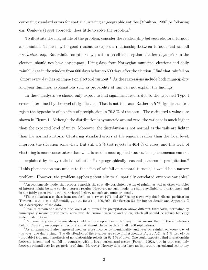
In these analyses we should only expect to find significant results due to the expected Type I

errors determined by the level of significance. That is not the case. Rather, a 5 % significance test

reject the hypothesis of no effect of precipitation in 70.8 % of the cases. The estimated t-values are

shown in Figure 1. Although the distribution is symmetric around zero, the variance is much higher

than the expected level of unity. Moreover, the distribution is not normal as the tails are lighter

than the normal kurtosis. Clustering standard errors at the regional, rather than the local level,

improves the situation somewhat. But still a 5 % test rejects in 46.4 % of cases, and this level of

clustering is more conservative than what is used in most applied studies. The phenomenon can not

be explained by heavy tailed distributions5 or geographically seasonal patterns in precipitation.6

If this phenomenon was unique to the effect of rainfall on electoral turnout, it would be a narrow

problem. However, the problem applies potentially to all spatially correlated outcome variables7

3An econometric model that properly models the spatially correlated patten of rainfall as well as other variablesof interest might be able to yield correct results. However, no such model is readily available to practitioners andin the fairly extensive literature reviewed below, no such attempts are made.

4The estimation uses data from ten elections between 1971 and 2007 using a two way fixed effects specificationTurnoutit = αi + τt + βsRainfalli,t+s + εit for s ∈ [−600, 600]. See Section 5.1 for further details and Appendix Cfor a description of the data.

5Results remain the same if one looks at dummies for precipitation above different thresholds, normalize bymunicipality means or variances, normalize the turnout variable and so on, which all should be robust to heavytailed distributions.

6Parliamentary elections are always held in mid-September in Norway. This means that in the simulationsbehind Figure 1, we compare precipitation at almost the same date in all 1200 replications.

7As an example, I also regressed median gross income by municipality and year on rainfall on every day ofthe year, one day a time. The distribution of the t-values are shown in Appendix Figure A-2. A 5 % test of the(probably) true null hypothesis of no relationship rejects on 62.5 % of days. One could expect to find a relationshipbetween income and rainfall in countries with a large agricultural sector (Paxson, 1992), but in that case onlybetween rainfall over longer periods of time. Moreover, Norway does not have an important agricultural sector any

3

Figure 1: Spurious t-values

0.0

2.0

4.0

6.0

8D

en

sity

−15 −10 −5 0 5 10t−value

Notes: The graph shows the coefficient from two way fixed effects regression of electoral turnouton a dummy for substantial daily precipitation. The dotted orange line shows the distributionwhen controlling for real election day rainfall whereas the solid green line excludes this variable.Standard errors are clustered at the municipal level. Precipitation for 600 days before to 600 daysafter election day employed, but data from +/- 10 days are excluded.

as well as explanatory variables exhibiting patterns similar to rainfall.8

As I argue below, the reason for this odd behavior is the presence of spatio-temporal tends

in the dependent variable: turnout in the eastern part of the country has decreased relative to

national averages whereas it has increased in relative terms in the western part. The underlying

explanation is probably differential development of macro-regional common factors. In some ways

this mimics the intricate spatial patterns detected in earnings data by Barrios et al. (2012), but

here also with a temporal component. In a stylized model with an omitted spatially correlated

variable, I show theoretically that OLS estimates are inconsistent with almost surely diverging

point estimates and t-statistics. Using Monte Carlo simulations, I further show that the test of

the irrelevance of the irrelevant variable is vastly over-rejected. This holds both with large sample

sizes, with several independent clusters of spatially dependent variables, using cross-sectional and

more.8The problem is not unique to rainfall. First, various terrain characteristics such as ruggedness and gradients, the

use of which was popularized by e.g. Duflo and Pande (2007), clearly exhibit spatial correlation. In the empiricalanalysis of violent conflict, for instance, researchers have found strong spatial and spatio-temoral patterns (seee.g. Buhaug and Gleditsch, 2008; Weidmann and Ward, 2010). There is also a vast literature on the spatial andspatio-temporal nature of housing and property prices (see e.g. Holly et al., 2011; Brady, 2014). More examplescould easily be listed. In all these cases, there is a danger of spurious relationships stemming from joint spatialpatterns.

4

panel data, as well as several specifications of the omitted trend including spatial AR processes.

Also, the simulations indicate that neither ordinary clustered standard errors nor Conley (1999)

standard errors solve the problem.

My suggested solution to the problem is to control for the trend using orthogonal polynomials.9

In the cross sectional spatial case, such a trend would be a polynomial in geographical coordinates.

In the case of panel data, we need a time trend whose slope varies geographically, so the slope of the

trend is modeled by a similar polynomial in geographical coordinates. Although any polynomial

can in theory be used, sequences of orthogonal polynomials have good numerical stability. In the

current study, I focus on tensor products of Legendre polynomials, which seem to perform well.

There are a few papers scrutinizing the validity of rainfall as an exogenous source of variation.

Sarsons (2015) look at the relationship between rainfall and conflict in India, where rainfall typically

is believed to be an instrument for income. However, she finds strong effects of rainfall both in

rain-fed and dam-fed regions, possibly invalidating this identification.

Methodologically, the present paper is also closely related to the work of Bertrand et al. (2004).

They show that differences in differences estimation tends to find effects effects of placebo “reforms”

on female wages. In one way, the present paper is a converse to their study as they focus on

outcomes with spatial patterns (wages) whereas I focus on explanatory variables with spatial

patterns. The study by Barrios et al. (2012) also indicate that failing to accounting for spatial

dependency may severely bias the results, but they also focus on standard errors.

The paper is also related to literature on spurious regressions in time series. It is well known

that the presence of non-stationary variables in regressions analyses can lead to spurious regression

(Granger and Newbold, 1974; Phillips, 1986). A less well known result is that this also holds for a

wide range of processes, including autocorrelated stationary processes (Granger et al., 2001; Kim

et al., 2004) – see Ventosa-Santaularia (2009) for a review. The problems I discuss are very similar,

but in the spatial domain.

Also, my suggested solution to estimate spatial or spatio-temporal trends relates to the lit-

erature on estimating time trends (Sims et al., 1990). As this concerns units in space, it also

9A number of papers using rainfall as an exogenous source of variation, e.g. Bruckner and Ciccone (2011) andFujiwara et al. (2016), also include spatially varying trends. However, it is not yet well understood why this isnecessary and hence the practice is not as widespread as it probably should be.

5

relates to the massive literature on spatial statistics10 and the more modest literature on spatial

econometrics.11 The literature on spatio-temporal statistics has a strong focus on space-time au-

toregressive moving average (STARMA) type models (Cliff et al., 1975; Pfeifer and Deutsch, 1980),

characterized by linear dependence lagged in both space and time. The literature on estimating

models with spatially dependent error terms is particularly relevant (Kelejian and Prucha, 1999;

Chudik et al., 2011; Pesaran and Tosetti, 2011). Such models can also be extended to regression

frameworks with spatial autoregressive distributed lags models (Elhorst, 2001). Although these

models may be suited to handle the problem at hand, their main problem is that they are difficult

to identify and estimate by themselves. When we also want to add panel data features, clustered

standard errors, instrumental variables or discontinuity designs, they become intractable and not

useful for practical applications. Hence I have chosen to rely on a simpler approach.

My suggested solution is to allow for a spatially varying time trend. This relates to the literature

on varying coefficients (Hastie and Tibshirani, 1993) and particularly spatially varying coefficients

(Gelfand et al., 2003). Specifically, Hoover et al. (1998) and Huang et al. (2002) estimate varying

coefficients models where they model the coefficients by regularized basis functions as I suggest

(albeit using B-splines rather than polynomial bases).12 However, they consider coefficients varying

in time, not in space. To the best of my knowledge, the only spatial application of the methodology

is Zhu et al. (2014) who study MRI images.

2 The problem

2.1 Rainfall regressions

The use of meteorological data in empirical analyses has skyrocketed in recent years.13 Some of

these take worries of spurious correlations into account by running placebo studies, but this is

not yet widespread. To both study the use of rainfall in applied empirical economics and see how

potential issues of spurious relationships are handled, I surveyed all articles published in three top

10Cressie (1993) and Ripley (2004) provide introductions to parts of the literature.11See e.g LeSage and Pace (2009) for an introduction.12See also Matsui et al. (2011, 2014) for some recent development.13See Dell et al. (2014) for a survey of parts of this literature.

6

economics journals in the period 2000-2017. See Appendix Table A-1 for the full list of articles.

In total, I found 45 articles. The earlier papers typically use data with coarse spatio-temporal

resolution whereas it becomes more common to rely on daily or even intra-daily data with high

spatial resolution over time. Clustering on spatial entities is also very common except in the

earliest papers, but only a few papers go any further in their treatment of spatial dependence

such as applying Conley (1999) standard errors. Moreover, only a handful of papers apply spatio-

temporal time trends that would alleviate the problems of spurious relationships studied herein.

Finally, I found only one paper (Madestam et al., 2013) that re-samples rainfall to check the

validity of their findings.

Starting with Gomez et al. (2007) and Hansford and Gomez (2010), there is also by now a

fairly large literature on the relationship between election day weather and turnout. Beyond the

US, the question has been studied in Japan, Holland, Spain, Italy, Sweden, Germany, Norway,

and South Korea (Horiuchi and Saito, 2009; Eisinga et al., 2012b,a; Artes, 2014; Sforza, 2013; Lo

Prete and Revelli, 2014; Persson et al., 2014; Arnold and Freier, 2016; Lind, 2014; Kang, 2018). In

many studies, it is found that rain on election day reduces turnout, but in Sweden there seems to

be essentially no relationship between the two and in Norway the relationship is positive. It has

also been argued that election day affects political outcomes either by affecting the composition

of voters (Gomez et al., 2007; Lind, 2014) or by affecting the preferences of voters (Meier et al.,

2016). Daily weather conditions have also been found to have an impact on participation in civil

rights riots in the 1960s (Collins and Margo, 2007), Tea Party rallies (Madestam et al., 2013), and

May day demonstrations (Kurrild-Klitgaard, 2013).

2.2 Other explanations

As already illustrated, regressions with rainfall as the independent variable seems to yield a dis-

tribution of t-values that differ markedly from the theoretical standard normal distribution. They

are not normally distributed,14 but the main problem is that the standard deviation is much higher

than unity. In the basic specification shown in Figure 1, the standard deviation of the t-statistics

14We can reject normality for all the t-values for all the four specification shown in Figure 2 using most conventionaltests and significance levels. The reason is mostly the low kurtosis.

7

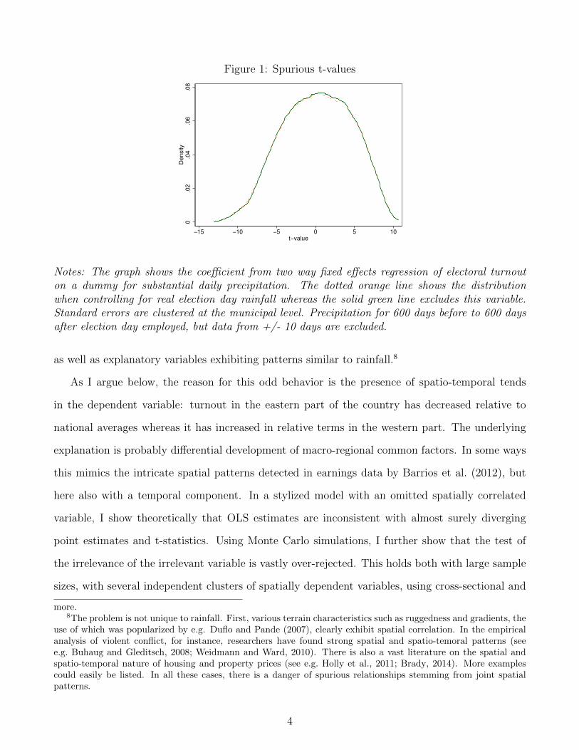
Figure 2: Distribution of the t-values0

.02

.04

.06

.08

Density

−15 −10 −5 0 5 10t−value

(a) No normalization0

.02

.04

.06

.08

Density

−15 −10 −5 0 5 10t−value

(b) Dummy for substantialrain

0.0

2.0

4.0

6.0

8.1

Density

−10 −5 0 5 10t−value

(c) Dummy for positive rain

0.0

2.0

4.0

6.0

8D

ensity

−20 −10 0 10 20t−value

(d) Measured as ranks

Notes: The graph shows the distribution of the t-values when regressing municipal turnout ondaily precipitation for 600 days before and after election day. The dotted orange line shows thedistribution when controlling for real election day rainfall whereas the solid green line excludes thisvariable. The 10 days before and after the actual election day are omitted. Panel (a) shows resultsfrom regressing levels on levels. Panel (b) shows the regression of turnout on a dummy for morethan 25 mm rain while Panel (c) employs a dummy for any rain. Panel (d) shows results froma regression where the rank of turnout is measured on the rank of rain, i.e. both variables areuniform on the unit interval.

is 4.37 – and a test of the hypothesis if it being unity rejects vastly.

Before exploring the explanation based on spatio-temporal trends further, it is worthwhile

dispensing with the alternative explanation of outliers in precipitation. It is well known that

rainfall data has a heavy right tail, which could affect the regression analyses. To show that this

cannot be the sole explanation, Figure 2 shows the distribution of the t-values in a number of

specifications that reduces the leverage of outliers. Panel (a) is the specification shown in the

introduction, where the level of turnout is regressed on the level of rain in millimeters. Panels (b)

and (c) replace the measure of precipitation with dummies for substantial rain, defined as above

2.5 mm, and any rain at all. Finally, in Panel (d) both rainfall and turnout are measured using

their ranks so they both have a uniform distribution on the unit interval. In all four cases, the

distribution of the test statistic is far from the standard normal or t-distributions we would expect.

This should indicate that mere outliers cannot explain the findings.

Another possible explanation could be spatially varying annual patterns in precipitation. Al-

though most Norwegian municipalities have higher average precipitation during winter than sum-

mer, there is some variation to the pattern which is spatially correlated. In a dataset with several

observations each year, this phenomenon can generate spurious correlations between rainfall and

8

Figure 3: Spatio-temporal patterns in turnout

Trend × 1000

under −5 −5 to −3 −3 to −1 −1 to 0 0 to 2 2 to 3

over 3

(a) Trends by municipality

●

●

●

●

●

● ●

●●

●

●

●

●

●●

●

●

● ●

●●

●

●

●

●

●●

●

●

●

●●

●

●●

●●

●

●●

●

●●

●

●

●

●

●

●

●

●

●

●

●●

●

●

●

●●

●

●

●

●

●●

●

●

●

●

●

●

●

●

●

●

●

●

●

●

●

●

●

●

●

●

●

●

●

●

●●

●

●

●

●

●

●

●

●

● ●

●

●

●

●● ●

●

●

●

● ● ●

●

●

●

●

●

● ●

●

●

●

●●

●

●

●

●

●

●●

●

●

●

●

●

●●

●

●

●

●

●

●

●

●

●

●

●●●

●

●

●●

●

●

●

●

●

●

●

●

●

●

●

●

●

●

●

●

● ●

●

●

●●

●

●

●●●

●

●

●

●

●

●

●

●

●

●

● ●●

●

●

●

●

●

●

● ●

●

●

●

● ●

●

●

●

●

●

●

●

●

●

●

●

●

●

●

●

●

●

●

●

●

●

●●

●

●

●

●

●

●

●

●

●●

●

●

●

●

●● ●

●

●

●

●

●

●

●

●

●

●

●

●

●

●

●

●

●

● ●

●

●

●●

●

●

●

●

●

●

●

●●

●

●

●

●

●

●

●

●

●

●

●

●

●

●

●

●●

●

●●

● ●

● ●

●

●●

●

●

●

●

●

●

●

●

●

●

●

●

●●

●

●

●

●

●●

●

●

●

●

●●

●

●

●

●●

● ●

●

● ●

●

●

●

●

●● ●

●

●●

●

●

●

●

●

●●

●

●

●

●

●

●

●

●

●

●

●

●

●

●

●

●

●

●

●

●

●

●

●

●

●

●●

● ●

●

●

●

●

●

●

●

●

●

●

●

●

●

●

●

●

●

●

●

●

●

●

●●

●

●

●

●

●

●

●

●

●

●

●

●●

●

−0.008 −0.006 −0.004 −0.002 0.000 0.002 0.004 0.006

−0.

006

−0.

004

−0.

002

0.00

0

Spatio−temporal trend

Spa

tio−

tem

pora

l tre

nd in

nei

ghbo

rs

(b) Trends in neighboring municipalities

Notes: The figure shows municipality specific coefficients δi from the regression (1). Red areas arestrong negative, blue areas strong positive.

other spatially correlated variables – and the problem would be easily solved by controlling for

seasonality. Parliamentary elections in Norway, however, are always held mid-September. Hence

on election days, municipalities are always at the same stage of their climatic seasonal cycle. In

the simulations, where we consider election day ±t days, we also end up with observations in

the same phase of the cycle. Consequently, seasonal patterns can not be the explanation for the

phenomenon.

2.3 Omitted spatially dependent variables

Rather, it seems that the nature of the problem is omitted variable exhibiting spatio-temporal

trends and potentially spatial non-stationarity15 in the rainfall data in combination with spatio-

15Spatial non-stationarity is commonly found in meteorological data even after demeaning, see e.g. Fuglstad et al.(2015) and Ingebrigtsen et al. (2015). However, to the best of my knowledge no general procedure for formallytesting for stationarity exists.

9

Table 1: Monte Carlo simulations based on actual rainfall

Mean Std. dev. Skewness Share rejected

1) No clustering 0.38 9.13 0.43 0.842) Clustered on region 0.25 3.41 1.20 0.593) Conley standard errors 0.18 3.15 0.62 0.594) Random municipality -0.04 1.00 0.17 0.055) Panel -0.62 7.96 0.12 0.81

Notes: The Table shows the results of Monte Carlo analyses simulating data as in (2) with εi ∼N(0, 1) and 1000 replications. All regressions are cross sectional analyses except the last row whichis based on a two way fixed effects panel data estimator. The cut offs for the Conley standard errorswere chosen as the standard deviation of the coordinates (longitude ±3.5, longitude ±5 degrees).

temporal trends in the turnout data. To explore the latter trends, I run a regression of the type

Turnoutit = αi + τt + δit+ εit (1)

Here δi is an estimate of the municipality specific trend. I have plotted the values of δi in Figure 3.

Panel (a) shows the geographical distribution of temporal trends. It is clear that there is a strong

negative trend in the eastern part of the country and a positive trend in parts of the west and

the center. Panel (b) shows a Moran plot where the municipality specific coefficient δi is plotted

against the average δi in the adjacent municipalities. Again it is clear that there is a spatial

pattern. Formally, Moran’s I statistic is I = 0.456 and the Moran test for no spatial dependency

rejects with a p-value of 2.2× 10−16. We conclude that when controlling for two way fixed effects,

turnout has been declining in the eastern part of the country and increasing in the western part.

As shown in Sections 3.1 and 3.2, this can explain the t-values shown in Figure 2.

Hence it seems that variables with spatial dependence may correlate spuriously with rainfall.

To show this more forcefully, I run some simulations. There are many ways of running these

simulations an obtaining spurious results. Here I have chosen a very simple specification which is

clearly nonsensical, and still correlates strongly with rainfall.

The independent variable is the observed rainfall in Norwegian municipalities on a random day

between January 1st 1968 and November 30th 2012.16 First, I consider a cross sectional setting

16See Appendix C for details on the meteorological data.

10

where I simulate dependent variables

zi = xi + yi + εi (2)

where xi and yi is the longitude and latitude of the municipal centre of municipality i and εi is a

standard normally distributed residual. Regressing zi on observed rainfall yields the results shown

in Row 1 of Table 1. The full distributions are shown in Appendix Figure A-3. As this is cross

sectional data, season patterns are not present in the data. As in the example above, we see

massive over rejection of false null hypotheses: Here the test at the 5 % level rejects in 84 % of

cases.

To account for the spatial pattern, I also attempt to cluster standard errors at the 19 regions

of Norway as well as using Conley (1999) standard errors. Both approaches seems to have about

the same effects of increasing the standard errors. However, as can be seen from Rows 2 and 3 of

Table 1, we still have rejection of the false null in 59 % of cases using a 5 % test. Moreover, we

notice that this tends to yield a heavily skewed distribution of the t-values. First, this indicates

that at least a substantial part of the problems lies in the estimated regression coefficient β, not

in the computation of the standard errors. In some ways, this is unsurprising as biased regression

coefficients are well known results from omitted variables problems. Second, it tells us that the

problem can not be solved by correcting the standard errors alone.

I also ran simulations as above, but where municipalities were assigned rainfall data from a

randomly selected municipality. This maintains the distribution of the independent variable but

removes the spatial pattern. As we can see from Row 4 of Table 1, we now get almost a perfect

replication of he standard normal distribution. This indicates that the cause of the problem is the

spatial correlations and not the skewed distribution of the rainfall data.

A typical way to control for such spatial patterns is to include municipal fixed effects, as

was done in the analysis of the turnout data above. As long as the dependent variable only

exhibits spatial correlation, this solves the problem. If, however, the variable has a spatially

dependent trend, fixed effects can’t solve the problem. To illustrate this, I draw panels starting

on a random day, with observations every four years and totally 10 observations per municipality.

11

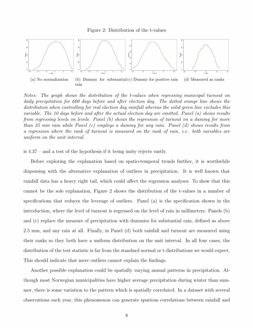
As all observations are on the same date, seasonal patterns are not present in the data. I then

construct a dependent variable as

yit = (xi + yi) t+ εit

Regressing yit on observed rainfall yields the results shown in Row 5 of Table 1. Again, the false

null is over rejected, this time in 81 % of cases for the 5 % test.

3 A general exposition of the problem

3.1 A theoretical approach

To get a better grasp of the nature of the problem at hand, I develop a simple econometric model

that is able to generate the phenomenon and may approximate the problem in real world situations.

The results of the model resemble those found by Granger et al. (2001) in the case of time series,

but certain features are better adapted to a spatial setting. Specifically, we want to show that

a spatially correlated explanatory variable that is in reality irrelevant may seem relevant – hence

generating a pattern of spurious correlation.

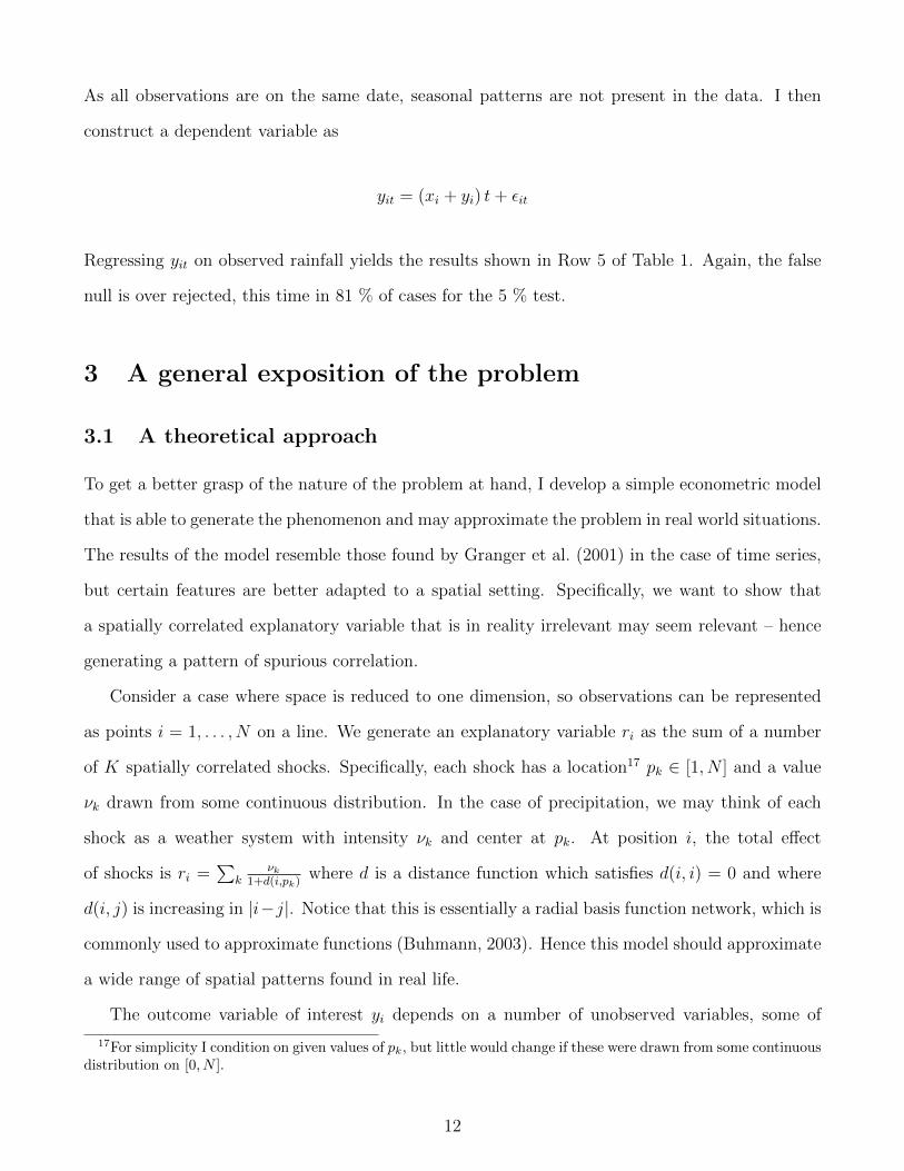
Consider a case where space is reduced to one dimension, so observations can be represented

as points i = 1, . . . , N on a line. We generate an explanatory variable ri as the sum of a number

of K spatially correlated shocks. Specifically, each shock has a location17 pk ∈ [1, N ] and a value

νk drawn from some continuous distribution. In the case of precipitation, we may think of each

shock as a weather system with intensity νk and center at pk. At position i, the total effect

of shocks is ri =∑

kνk

1+d(i,pk)where d is a distance function which satisfies d(i, i) = 0 and where

d(i, j) is increasing in |i−j|. Notice that this is essentially a radial basis function network, which is

commonly used to approximate functions (Buhmann, 2003). Hence this model should approximate

a wide range of spatial patterns found in real life.

The outcome variable of interest yi depends on a number of unobserved variables, some of

17For simplicity I condition on given values of pk, but little would change if these were drawn from some continuousdistribution on [0, N ].

12

Figure 4: The stylized econometric model

0.5

11.

5r i

020

4060

8010

0y i

0 20 40 60 80 100i

(a) The set up

020

4060

8010

0y i

0 .5 1 1.5ri

(b) The relationship

Notes: Panel (a) shows the simulated yi and riagainst the observation number i. Panel (b) showsa scatter plot of yi versus ri as well as a linear fit of the data. Data are simulated for β = 0.

which are spatially correlated. In the theoretical exposition, we model these are resulting in a

spatial trend τi for some trend parameter τ , so the outcome variable is given by

yi = α + βri + τi+ εi. (3)

We may suspects that ri also enters equation (3) with a slope β. Hence we want to test the

hypothesis that β = 0. Using conventional tools, we would disregard the spatial trend τi. The

core of the problem, as we see below, is that a regression of yi on ri mixes up the trend τi and the

signal ri.

In the theoretical exposition, I focus on the metric d(i, j) = |i− j| and the case with only one

shock p, i.e. K = 1. This case is illustrated in Figure 4. As is apparent from the figure, whenever

the “position” of the shock is p 6= N2

, there is scope for the shock to pick up parts of the trend.

We want to show this formally and see how a test is affected by an increasing sample size N . It

turns out that in this case, the problem does not diminish but rather get more acute.

When the data are generated as in equation (3), but where we fail to control for the trend τi

13

in the analysis, the OLS estimator becomes

β = β +1N

∑(ri − r)εi

1N

∑(ri − r)2

+ τ1N

∑(ri − r)i

1N

∑(ri − r)2

(4)

When εi ∼ iid (0, σ2) the first fraction converges in distribution to a well behaved normally

distributed term by application of the central limit theorem. This is handled by ordinary estimation

and hypothesis testing procedures. The second term, which stems from the omitted variable,

however, is the root of the problem. In finite samples it it non-zero unless p = N2

. Moreover, the

problem is exacerbated with growing sample sizes, as the following result demonstrates:

Proposition 1. When N → +∞ and KN→ κ < +∞, we have Pr

(∣∣∣β − β∣∣∣→ +∞)

= 1.

The full proof is provided in Appendices B.1 and B.2. Denote by w the average

w = 1N

∑Ni=1

∑Kk=1

11+|pk−i|

. In Appendix B.1 I show that the expression 1N

∑Ni=1

∑Kk=1

(1

1+|pk−i|− w

)i

converges to a logarithmic function and hence diverges as N → ∞. The proof is based on show-

ing that the expression can be sandwiched between two harmonic sequences which both have

logarithmic growth. Moreover, in Appendix B.2 I show that if KN→ κ ∈ R+, we have that as

N → ∞, the denominator 1N

∑Ni=1

∑Kk=1

(1

1+|pk−i|− w

)2

→ Q ∈ R+. This is based on showing

that∑N

i=1

∑Kk=1

(1

1+|pk−i|− w

)2

is closely related to the sum of reciprocals of squares of natural

numbers. The sum of this sequence is known to converge to π2

6. As a consequence, the sum at

hand also converges to a constant. Consequently, the expression goes to 0 at rate O(

1N

). If on

the other hand we allow K to grow linearly as N grows, the denominator converges to a constant.

In both cases, the estimator β explodes and hence is inconsistent. However, unlike conventional

omitted variables biases, the sign of the bias is random.

In applied research much emphasis is on statistical significance, i.e. the t-values. As the

denominator in (4) converges to a constant, the standard error of β also converge to a constant.

As β−β diverges, this implies that the t-values also diverge. This could hence explain the unusually

high t-values observed above.

One objection to this analysis could be that as N increases, the size of space, and hence the

range of ri, increases. An alternative model could be to restrict space to say [0, 1] and increase the

14

density of observations as N increases. Then the trend should be modeled as τiN

, and the distance

metric for the shocks replaced by∣∣ iN− pk

N

∣∣. However, it is easily seen that in computing OLS

estimates, this does not change the final expression and hence the regression estimate still diverges

as N increases.

The above results depends on the the specification of ri being proportional to the inverse of the

distance. If the weighting decays more quickly, a may be realistic in many applications, the proof

of divergence has to be changed.18 However, it seems that the main insight would go through with

other specifications of the weighting too.

3.2 Monte Carlo evidence

The results presented in Section 3.1 apply to a stylized model. To illustrate that these results

are more general, I now report results from a number of Monte Carlo analyses on varieties of this

model.

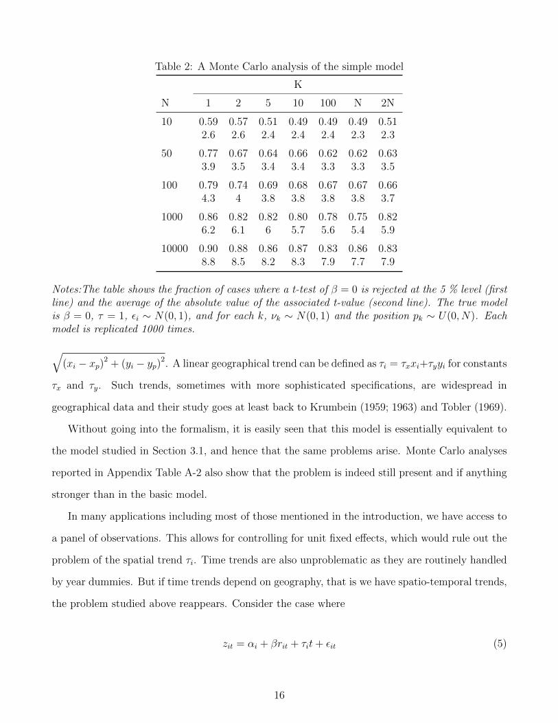
Table 2 shows a Monte Carlo analysis of the model from Section 3.1 for sample sizes between

10 and 10000 and number of shocks varying from 1 to 20000. The simulations are based on a

model where the true β = 0 so the fraction of t-tests rejecting the null should correspond to the

level of the test, here 5 %. First, we recognize the diverging t-values: The larger the sample gets,

the more likely the t-test is to reject. The test at the 5 % level rejects in about half of the cases

for small samples and in more than 80 % of cases in larger samples. 19 Rejections rates and values

of |t| are slightly smaller for larger numbers of shocks, but this is not enought to take levels down

to reasonable magnitudes.

In many real world applications, the assumption of a linear world is too restrictive.20 A more

realistic assumption is a spatial data structure where it is meaningful to talk about the distance

between two observations, and where units tend to be correlated with nearby units. Denoting

observation i’s geographical position (xi, yi), we can use the Euclidean distance function d(i, p) =

18Typically one can show that although the numerator in (4) converges to zero, the denominator converges at ahigher rate so the fraction diverges.

19These numbers could of course be reduced by increasing the noise, i.e. increasing the variance of εi, but thisdoes not reduce the importance of the problem.

20An exception is time series data, but the current modeling of shocks does not seem particularly relevant to thatcase.

15

Table 2: A Monte Carlo analysis of the simple model

K

N 1 2 5 10 100 N 2N

10 0.59 0.57 0.51 0.49 0.49 0.49 0.512.6 2.6 2.4 2.4 2.4 2.3 2.3

50 0.77 0.67 0.64 0.66 0.62 0.62 0.633.9 3.5 3.4 3.4 3.3 3.3 3.5

100 0.79 0.74 0.69 0.68 0.67 0.67 0.664.3 4 3.8 3.8 3.8 3.8 3.7

1000 0.86 0.82 0.82 0.80 0.78 0.75 0.826.2 6.1 6 5.7 5.6 5.4 5.9

10000 0.90 0.88 0.86 0.87 0.83 0.86 0.838.8 8.5 8.2 8.3 7.9 7.7 7.9

Notes:The table shows the fraction of cases where a t-test of β = 0 is rejected at the 5 % level (firstline) and the average of the absolute value of the associated t-value (second line). The true modelis β = 0, τ = 1, εi ∼ N(0, 1), and for each k, νk ∼ N(0, 1) and the position pk ∼ U(0, N). Eachmodel is replicated 1000 times.

√(xi − xp)2 + (yi − yp)2. A linear geographical trend can be defined as τi = τxxi+τyyi for constants

τx and τy. Such trends, sometimes with more sophisticated specifications, are widespread in

geographical data and their study goes at least back to Krumbein (1959; 1963) and Tobler (1969).

Without going into the formalism, it is easily seen that this model is essentially equivalent to

the model studied in Section 3.1, and hence that the same problems arise. Monte Carlo analyses

reported in Appendix Table A-2 also show that the problem is indeed still present and if anything

stronger than in the basic model.

In many applications including most of those mentioned in the introduction, we have access to

a panel of observations. This allows for controlling for unit fixed effects, which would rule out the

problem of the spatial trend τi. Time trends are also unproblematic as they are routinely handled

by year dummies. But if time trends depend on geography, that is we have spatio-temporal trends,

the problem studied above reappears. Consider the case where

zit = αi + βrit + τit+ εit (5)

16

with the trend τi = τxxi + τyyi for constants τx and τy. If we assume a balanced panel so we can

differentiate expression (5), we get

∆zit = β∆rit + τi + ∆εit

which essentially is specification (3). De-meaning of course yields similar results. The only major

difference is that we look at differenced shocks (or deviations from means). However, these have

the exact same properties of spatial correlation as the undifferenced shock, so the issues studied in

Section 3.1 still remain. Monte Carlo simulations of this model also yield very similar conclusions

– the null hypothesis of no relationship which should have been rejected in 5% of cases is rejected

far too often and t-values are typically high.21 Moreover, the problem is exacerbated by increasing

sample sizes. There are some indications that increased panel lengths reduces the problem. As

time periods are independent of each other, increasing T increases the (random) variation in ∆ri

which helps uncover its independence to ∆zit.

The mechanism generating the spurious rejections of hypothesis tests above is that the precip-

itation shocks in sum are non-zero and with opposite sign in different corners of space. With a

spatial trend, the two combines to form spurious correlation. The assumption of a deterministic

spatial (or spatio-temporal) trend may be too strong in certain applications. However, the problem

may persist in more general models of spatial dependence.

Consider a model in one-dimensional space of the form

yi = α + βri + ui

ui = ρui−1 + εi,

(6)

i.e. a simple first order auto-regressive model.22 Unbiased test of the hypothesis β = 0 depends

on E∑

i riui = 0. With the current specification, we have ui =∑i−1

j=0 ρjεi. Say for simplicity that

21See Appendix Table A-3 for details.22To simplify, correlation is only to the left. The model would be essentially unchanged if ui was correlated with

both ui−1 and ui+1.

17

the location p is at an integer. Then

∑i

riui =

N−p∑j=0

ν

1 + juj+p +

p−1∑j=1

ν

1 + jup−j.

Using the autoregressive structure of the residuals, this can be rewritten

∑i

riui =N∑i=1

εi

N−1∑j=0

ν

1 + |p− i+ j|ρj.

With high spatial dependence (i.e. ρ close to unity), the loading on a few of the innovations εi

close to p is going to be large, and these innovations determine the whole estimated β. Even as N

gets large, this effect persists.

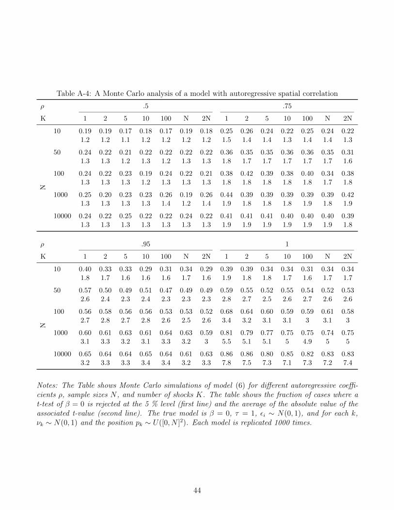
For K > 1, we compare the loading on εi around several clusters. Still, some of the clusters

dominate and hence the bias remains the same if not worse.23 Moreover, when the spatial de-

pendency is high (ρ is close to unity), we get spurious relationships in the vast majority of cases.

Increasing the sample size or the number of shocks does not seem to improve the situation.

4 Detecting and solving the problem

In the case of the weather, the problem of spurious correlations can usually be detected by exam-

ining the weather at counterfactual dates as in Figure 1. With other independent variables, other

placebos may be feasible. If rejection rates differ markedly from the expected rates, some spatial

or spatio-temporal dependency may be the explanation although of course other explanations ob-

viously also exist. The next step should be to try to get some impression of the spatial dependency.

One way to do this is to simply plot maps of spatial values or estimated spatial trends. In some

cases it may also be useful to use testing procedures such as Moran’s I statistic.

If a spatial pattern is found, two possible solutions can be pursued. The ideal solution is to

find the source of the dependency and expand the model specification to take this into account.

If, for instance, geographically varying trends are due to geographical differences in demographic

23Results are reported in Appendix Table A-4

18

patterns (say young people moving toward large cities), one could potentially solve the problem

by adding demographic controls. However, it may not always be easy to find a simple explanation

and there may not be a single explanation for the geographical trend. In such cases, it may be a

better option to attempt to control for the geo-spatial trend. In the time series literature, this is

usually done by simply including the date as a variable, sometimes with a few polynomial terms.

In the case of geographical data, this may be too limiting.

In the cross sectional case, we want to control for some unknown function T (x, y). As the

shape of T is unknown, a flexible estimator in two-dimensional space is called for. Kernel based

and other standard non-parametric estimators are computationally intensive, and as their rate of

convergence is typically below√n, inference of the other variables in the regression can’t always

be made using standard techniques. Consequently, a simpler form may be advisable.

In the case of a panel, we need to estimate a function T (x, y, t). As this is a function of three

variables, a fully flexible non-parametric approach gets even more demanding. At least for short

panels, it seems reasonable that the trend may be kept linear, so we can rewrite T (x, y, t) = U(x, y)t

for some function U . One solution that seems to work well for the electoral turnout data considered

below is one where U is specified as a tensor product of Legendre polynomials.24 The choice of

orthogonal polynomials is to reduce problems of multicollinearity and improve numerical stability.

One justification for choosing Legendre polynomials is their orthogonality property with regard

to an L2 inner product given a uniform spatial distribution of units. Although the distribution

is not exactly uniform, this approach is likely to give better behavior than most other orthogonal

polynomial bases that provide orthogonality given various bell shaped distributions. Still, it seems

that the choice of polynomial base has little effect on the final outcomes.

Given dimensionalities K and L, we can specify

T (x, y, t) = t

K∑k=0

L∑`=0

θk`Pk (x)P` (y) (7)

where Pi(·) is the i’th order Legendre polynomial.25 The (K + 1)(L + 1) parameters θk` can be

24See e.g. Judd (1998, Ch. 6) for an overview of Legendre polynomials and other polynomial basis with applica-tions in economics and Totik (2005) for the mathematical background.

25These polynomials are usually defined recursively with P0(x) = 1, P1(x) = x, and for i ≥ 2, Pi(x) =

19

estimated together with the other parameters in an ordinary regression model.

The choice of the dimensions K and L has to be chosen to make the polynomial (7) provide a

reasonable fit of the data. If K and L are chosen too high, there is both a danger of over fitting

(Hastie et al., 2008, Ch. 7) and loosing so much variation that it becomes impossible to identify

the effect of the variable of interest. Hence we want would like a good fit with a low dimensional

polynomial. To make a good trade off, I recommend to consider choosing K and L by maximizing

a linear penalty function

R2 − ξ(K + 1)(L+ 1) (8)

where R2 is the fit of the model and ξ a penalty on the number of parameters to estimate. This is

closely related to maximizing the AIC and BIC criteria, but varying the degrees of freedom penalty.

Varying the parameter ξ, we can trace out the class of potentially good polynomial compositions.

It is also important to undertake counter factual estimations as in Figure 1 to check that the

polynomial at hand actually solves the problem. If the fit is good enough, most of the placebo

variables should have little effect on the outcome. Another approach could also be to choose K

and L high, but constrain the θk` by employing ridge regression, LASSO, or other versions of

constrained estimation (Belloni et al., 2014; Hastie et al., 2008, Ch. 3).

5 Turnout in Norwegian elections

Let us now return to the application considered in the introduction, the effect of rainfall on electoral

turnout in Norwegian municipal elections. The data are described in Appendix C.

5.1 Specifying the spatio-temporal trend

As argued in Section 4, one way to handle the problem of spation-temporal trends is to control them

out in the estimation. I approximate the trend with the tensor product of Legendre polynomials.

The first step needed is to make a choice of how many polynomial terms to include in each of the two

[(2i− 1)xPi−1(x)− (i− 1)Pi−1(x)] /i where the variable x is normalized to be in the interval [−1, 1].

20

Figure 5: The number of terms in the nonparametric trend model0

24

68

10Lo

ngitu

de te

rms

0 2 4 6 8 10Lattitude terms

0.005.01.015.02.025.03.035.04.045.05.055.06.065.07.075.08.085.09.095.1.105

Incr

ease

d fit

(a) Model fit and number of longiude and latitudeterms

0.0

2.0

4.0

6.0

8.1

Incr

ease

d fit

0 20 40 60 80 100 120Total number of terms

(b) Model fit and total number of terms

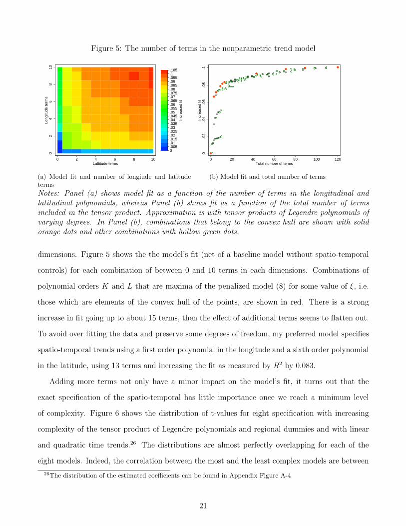
Notes: Panel (a) shows model fit as a function of the number of terms in the longitudinal andlatitudinal polynomials, whereas Panel (b) shows fit as a function of the total number of termsincluded in the tensor product. Approximation is with tensor products of Legendre polynomials ofvarying degrees. In Panel (b), combinations that belong to the convex hull are shown with solidorange dots and other combinations with hollow green dots.

dimensions. Figure 5 shows the the model’s fit (net of a baseline model without spatio-temporal

controls) for each combination of between 0 and 10 terms in each dimensions. Combinations of

polynomial orders K and L that are maxima of the penalized model (8) for some value of ξ, i.e.

those which are elements of the convex hull of the points, are shown in red. There is a strong

increase in fit going up to about 15 terms, then the effect of additional terms seems to flatten out.

To avoid over fitting the data and preserve some degrees of freedom, my preferred model specifies

spatio-temporal trends using a first order polynomial in the longitude and a sixth order polynomial

in the latitude, using 13 terms and increasing the fit as measured by R2 by 0.083.

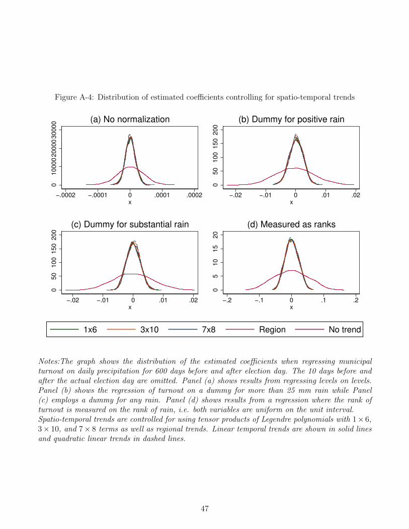
Adding more terms not only have a minor impact on the model’s fit, it turns out that the

exact specification of the spatio-temporal has little importance once we reach a minimum level

of complexity. Figure 6 shows the distribution of t-values for eight specification with increasing

complexity of the tensor product of Legendre polynomials and regional dummies and with linear

and quadratic time trends.26 The distributions are almost perfectly overlapping for each of the

eight models. Indeed, the correlation between the most and the least complex models are between

26The distribution of the estimated coefficients can be found in Appendix Figure A-4

21

.85 and .9.

Moreover, we notice that the distribution of t-values is much more well behaved than the

t-values obtained without controlling for spatio-temporal trends. Although the distribution is

somewhat fatter than the theoretical Student’s t distribution, the distribution is much more sensible

to work with.

Finally, it seems that using region specific trends has a comparable effect in improving es-

timation results to spatio-temporal trends. As argued above there are many cases where it is

implausible that the trend has a spatial discontinuity at regional borders. Still, it seems that this

potential mis-specification has little impact in practice.

5.2 The effect of rainfall on turnout

Table 3 shows the actual estimation results regressing turnout on election day weather. First,

specifications (1) and (2) show the estimation results using a two-way fixed effects specification

without controlling for spatio-temporal trends. The simplest specification indicate that rainfall

does not affect turnout. When we interact rainfall with a time trend, it seems that rainfall suddenly

has a time-varying effect. In Panel A of Appendix Table A-5 I show some additional specifications,

where signs and significance levels are even more erratic. As argued above, this specification is

probably not trustworthy.

In specifications (3) and (4) of Table 3, I show the estimation results from the preferred speci-

fications. The general pattern is that rain seems to increase turnout in Norway – see Lind (2014)

for a discussion of the rationale behind this. Column (1) shows the plain regression of turnout

on precipitation in cm. The effect of 1 cm increase in precipitation is about .3 percentage point

increase in turnout. Columns (2) includes a time interaction. We see that with this specification,

the results seem to be stable over time as the interaction is insignificant. In Panel B of Appendix

Table A-5 I include the same specifications as above. Now, the picture arising is homogenous

across specifications indicating a much more stable specification.

22

Figure 6: Distribution of t-values controlling for spatio-temporal trends

0.0

5.1

.15

.2

−15 −10 −5 0 5 10x

(a) No normalization

0.0

5.1

.15

.2.2

5

−10 −5 0 5 10x

(b) Dummy for positive rain

0.0

5.1

.15

.2

−15 −10 −5 0 5 10x

(c) Dummy for substantial rain0

.05

.1.1

5

−10 0 10 20x

(d) Measured as ranks

1x6 3x10 7x8 Region No trend

Notes:The graph shows the distribution of the t-values when regressing municipal turnout on dailyprecipitation for 600 days before and after election day. The 10 days before and after the actualelection day are omitted. Panel (a) shows results from regressing levels on levels. Panel (b) showsthe regression of turnout on a dummy for more than 2.5 mm rain while Panel (c) employs a dummyfor any rain. Panel (d) shows results from a regression where the rank of turnout is measured onthe rank of rain, i.e. both variables are uniform on the unit interval.Spatio-temporal trends are controlled for using tensor products of Legendre polynomials with 1× 6,3 × 10, and 7 × 8 terms as well as regional trends. The graph also includes the t-values obtainedwithout spatio-temporal trends. Linear temporal trends are shown in solid lines and quadratic lineartrends in dashed lines.

23

Table 3: The effect of precipitation on turnout

Without trend With trend

(1) (2) (3) (4)

Rain (in cm) -0.000339 0.00134** 0.00299*** 0.00283***(-0.50) (2.46) (5.34) (5.29)

Rain positive

Rain above 2.5 mm

Rain × Year 0.00185*** -0.000356(6.96) (-1.56)

Mean dep. var 0.681 0.681 0.681 0.681Obs 4417 4417 4417 4417R2 0.612 0.624 0.698 0.698

Notes: Outcome variable is municipal electoral turnout. All specifications include municipal andyear fixed effects. Specifications (3) and (4) also include the tensor product of Legendrepolynomials with 1× 6 terms to control for spatio-temporal trends. Standard errors are clusteredat the municipality level (using the 2010 municipal structure).t-values in parentheses,and *, **, and *** denotes significant at the 10%, 5%, and 1% levels.

24

6 Conclusion

In this paper, I have shown that when outcomes of interest are regressed on weather data, there is

a danger of spuriously detecting relationships. To illustrate the occurrence of the problem, I have

shown nonsensical relationships such as a relationship between electoral turnout and rainfall 100

days before the election. In such cases, the relationship can be rejected by common sense. But for

more relevant questions, such as whether rain on the day of the election affect turnout, the problems

of spatial correlation remain the same. To give a satisfactory answer in the potentially interesting

cases, we need a proper understanding of the phenomena generating the spurious relationships.

The reason for these relationships, I argue, is that spatial patterns in weather conditions are

likely to align up with spatial or spatio-temporal patterns in the outcomes of interest. I have shown

that this does indeed occur in a simple model of spatially dependent data as well as in an extensive

range of Monte Carlo analyses. Moreover, the analyses reveal that standard techniques, such as

clustering on spatial entities (Moulton, 1986) or using Conley’s (1999) approach to computing

standard errors does solve the problem.

Rather, I suggest introducing controls for spatial or spatio-temporal trends in regressions to

solve the problem. This is a simple remedy that can easily be combined with other techniques, such

as instrumental variables of regression discontinuity designs. In a sample of Norwegian municipal

elections, I show that this reduces the problem of spurious relationships in statistical tests to close

to the theoretical properties.

The question of more sophisticated approaches to controlling for spatial and spatio-temporal

trends, possibly borrowing from the literature on spatial statistics and econometrics is left for future

research. There are probably possibilities to do better, but it is unclear that such approaches are

sufficiently simple to implement that they actually matter for the applied researcher.

In studies of the effect of short term weather changes, as studied in this paper, weather data

are typically available for a large number of periods, of which only a few matter. Then there is

ample supply of placebo data. Such data should regularly be used to test the validity of empirical

approaches used. In studies of the effect of long term weather effects, such as the effect on

agricultural production, surplus data are harder to find. Still it may be possible to run placebo

25

studies by temporally moving the whole or parts of the rainfall pattern.

When placebo data can be constructed, one may also ask whether these they could be used to

construct a more correct null distribution of the parameter of interest, somewhat along the lines of

bootstrapping techniques. Saunders (1993) implements a version of this estimator, but does not

go into its statistical properties and potential advantages compared to ordinary inference.

References

Arnold, F. and R. Freier (2016): “Only conservatives are voting in the rain: Evidence from

German local and state elections,” Electoral Studies, 41, 216 – 221.

Artes, J. (2014): “The rain in Spain: Turnout and partisan voting in Spanish elections,” European

Journal of Political Economy, 34, 126 – 141.

Barrios, T., R. Diamond, G. W. Imbens, and M. Kolesar (2012): “Clustering, Spatial

Correlations, and Randomization Inference,” Journal of the American Statistical Association,

107, 578–591.

Belloni, A., V. Chernozhukov, and C. Hansen (2014): “Inference on Treatment Effects

after Selection among High-Dimensional Controls,” The Review of Economic Studies, 81, 608–

650.

Bertrand, M., E. Duflo, and S. Mullainathan (2004): “How Much Should We Trust

Differences-In-Differences Estimates?” The Quarterly Journal of Economics, 119, 249–275.

Brady, R. R. (2014): “The spatial diffusion of regional housing prices across U.S. states,” Re-

gional Science and Urban Economics, 46, 150 – 166.

Bruckner, M. and A. Ciccone (2011): “Rain and the Democratic Window of Opportunity,”

Econometrica, 79, 923–947.

Buhaug, H. and K. S. Gleditsch (2008): “Contagion or Confusion? Why Conflicts Cluster

in Space1,” International Studies Quarterly, 52, 215–233.

26

Buhmann, M. D. (2003): Radial basis functions: theory and implementations, Cambridge Uni-

versity Press.

Chudik, A., M. H. Pesaran, and E. Tosetti (2011): “Weak and strong cross-section depen-

dence and estimation of large panels,” The Econometrics Journal, 14, C45–C90.

Cliff, A. D., P. Haggett, J. K. Ord, K. A. Bassett, and R. B. Davies (1975): Elements

of Spatial Structure: A Quantitative Approach, Cambridge University Press.

Collins, W. J. and R. A. Margo (2007): “The Economic Aftermath of the 1960s Riots

in American Cities: Evidence from Property Values,” The Journal of Economic History, 67,

849–883.

Conley, T. (1999): “GMM estimation with cross sectional dependence,” Journal of Economet-

rics, 92, 1 – 45.

Cressie, N. A. C. (1993): Statistics for Spatial Data, John Wiley & Sons.

Dell, M., B. F. Jones, and B. A. Olken (2014): “What Do We Learn from the Weather?

The New Climate-Economy Literature,” Journal of Economic Literature, Forthcoming.

Duflo, E. and R. Pande (2007): “Dams,” The Quarterly Journal of Economics, 122, 601–646.

Eisinga, R., M. Grotenhuis, and B. Pelzer (2012a): “Weather conditions and political

party vote share in Dutch national parliament elections, 1971-2010,” International Journal of

Biometeorology, 56, 1161–1165.

——— (2012b): “Weather conditions and voter turnout in Dutch national parliament elections,

1971-2010,” International Journal of Biometeorology, 56, 783–786.

Elhorst, J. P. (2001): “Dynamic Models in Space and Time,” Geographical Analysis, 33, 119–

140.

Fiva, J. H., A. Halse, and G. J. Natvik (2012): “Local Government Dataset,” Dataset

available from http://www.jon.fiva.no/data/FivaHalseNatvik2015.zip.

27

Fuglstad, G.-A., D. Simpson, F. Lindgren, and H. Rue (2015): “Does non-stationary

spatial data always require non-stationary random fields?” Spatial Statistics, 14, Part C, 505–

531.

Fujiwara, T., K. C. Meng, and T. Vogl (2016): “Habit Formation in Voting: Evidence

from Rainy Elections,” American Economic Journal: Applied Economic, Forthcoming.

Gelfand, A. E., H.-J. Kim, C. F. Sirmans, and S. Banerjee (2003): “Spatial Modeling

with Spatially Varying Coefficient Processes,” Journal of the American Statistical Association,

98, 387–396.

Gomez, B. T., T. G. Hansford, and G. A. Krause (2007): “The Republicans Should Pray

for Rain: Weather, Turnout, and Voting in U.S. Presidential Elections,” The Journal of Politics,

69, 649–663.

Granger, C. and P. Newbold (1974): “Spurious regressions in econometrics,” Journal of

Econometrics, 2, 111 – 120.

Granger, C. W. J., N. Hyung, and Y. Jeon (2001): “Spurious regressions with stationary

series,” Applied Economics, 33, 899–904.

Hansford, T. G. and B. T. Gomez (2010): “Estimating the Electoral Effects of Voter

Turnout,” American Political Science Review, 104, 268–288.

Hastie, T. and R. Tibshirani (1993): “Varying-Coefficient Models,” Journal of the Royal

Statistical Society. Series B (Methodological), 55, 757–796.

Hastie, T., R. Tibshirani, and J. Friedman (2008): The elements of statistical learning:

data mining, inference and prediction, Springer, 2 ed.

Holly, S., M. H. Pesaran, and T. Yamagata (2011): “The spatial and temporal diffusion

of house prices in the UK,” Journal of Urban Economics, 69, 2 – 23.

Hoover, D. R., J. A. Rice, C. O. Wu, and L.-P. Yang (1998): “Nonparametric smoothing

estimates of time-varying coefficient models with longitudinal data,” Biometrika, 85, 809–822.

28

Horiuchi, Y. and J. Saito (2009): “Rain, Election, and Money: The Impact of Voter Turnout

on Distributive Policy Outcomes,” Mimeo, Yale (http://ssrn.com/abstract=1906951).

Huang, J. Z., C. O. Wu, and L. Zhou (2002): “Varying-coefficient models and basis function

approximations for the analysis of repeated measurements,” Biometrika, 89, 111–128.

Ingebrigtsen, R., F. Lindgren, I. Steinsland, and S. Martino (2015): “Estimation of a

non-stationary model for annual precipitation in southern Norway using replicates of the spatial

field,” Spatial Statistics, 14, Part C, 338–364.

Judd, K. L. (1998): Numerical methods in economics, MIT Press.

Kang, W. C. (2018): “The Liberals Should Pray for Rain: Weather, Opportunity Costs of Voting

and Electoral Outcomes in South Korea,” Mimeo, ANU.

Kelejian, H. H. and I. R. Prucha (1999): “A Generalized Moments Estimator for the Au-

toregressive Parameter in a Spatial Model,” International Economic Review, 40, 509–533.

Kim, T.-H., Y.-S. Lee, and P. Newbold (2004): “Spurious regressions with stationary pro-

cesses around linear trends,” Economics Letters, 83, 257–262.

Koopmans, T. C. (1949): “Identification Problems in Economic Model Construction,” Econo-

metrica, 17, 125–144.

Krumbein, W. C. (1959): “Trend surface analysis of contour-type maps with irregular control-

point spacing,” Journal of Geophysical Research, 64, 823–834.

——— (1963): “Confidence intervals on low-order polynomial trend surfaces,” Journal of Geo-

physical Research, 68, 5869–5878.

Kurrild-Klitgaard, P. (2013): “It’s the weather, stupid! Individual participation in collective

May Day demonstrations,” Public Choice, 155, 251–271.

LeSage, J. and R. K. Pace (2009): Introduction to Spatial Econometrics, CRC Press.

29

Lind, J. T. (2014): “Rainy Day Politics - An Instrumental Variables Approach to the Effect of

Parties on Political Outcomes,” CESifo Working Paper No. 4911.

Lo Prete, A. and F. Revelli (2014): “Voter Turnout and City Performance,” SIEP Working

Paper 10 (http://www.siepweb.it/siep/images/joomd/1415351423LoPrete Revelli WP SIEP 676.pdf).

Madestam, A., D. Shoag, S. Veuger, and D. Yanagizawa-Drott (2013): “Do Political

Protests Matter? Evidence from the Tea Party Movement,” Quarterly Journal of Economics,

128, 1633–85.

Matsui, H., T. Misumi, and S. Kawano (2011): “Varying-coefficient modeling via regularized

basis functions,” ArXiv e-prints.

——— (2014): “Model selection criteria for the varying-coefficient modelling via regularized basis

expansions,” Journal of Statistical Computation and Simulation, 84, 2156–2165.

Meier, A. N., L. D. Schmid, and A. Stutzer (2016): “Rain, Emotions and Voting for the

Status Quo,” IZA Discussion Paper 10350.

Miller, B. M. (2015): “Does Validity Fall from the Sky? Observant Farmers and the Endogeneity

of Rainfall,” Mimeo, UC San Diego.

Mohr, M. (2008): “New Routines for Gridding of Temperature and Precipitation Observations

for ”seNorge.no”,” Tech. rep., met.no note 08/2008.

Moulton, B. R. (1986): “Random group effects and the precision of regression estimates,”

Journal of Econometrics, 32, 385–397.

Paxson, C. H. (1992): “Using weather variability to estimate the response of savings to transitory

income in Thailand,” American Economic Review, 82, 15–33.

Persson, M., A. Sundell, and R. Ohrvall (2014): “Does Election Day weather affect voter

turnout? Evidence from Swedish elections,” Electoral Studies, 33, 335–342.

Pesaran, M. H. and E. Tosetti (2011): “Large panels with common factors and spatial

correlation,” Journal of Econometrics, 161, 182–202, cited By 61.

30

Pfeifer, P. E. and S. J. Deutsch (1980): “A three-stage iterative procedure for space-time

modeling,” Technometrics, 22, 35–47.

Phillips, P. C. B. (1986): “Understanding spurious regressions in econometrics,” Journal of

Econometrics, 33, 311 – 340.

Ripley, B. D. (2004): Spatial Statistics, John Wiley & Sons, 2nd ed.

Sarsons, H. (2015): “Rainfall and conflict: A cautionary tale,” Journal of Development Eco-

nomics, 115, 62 – 72.

Saunders, Jr, E. M. (1993): “Stock Prices and Wall Street Weather,” The American Economic

Review, 83, 1337–1345.

Sforza, A. (2013): “The Weather Effect: Estimating the effect of voter turnout on

electoral outcomes in Italy,” Mimeo, London School of Economics and Political Sciences

(http://www.bportugal.pt/pt-PT/BdP

Sims, C. A., J. H. Stock, and M. W. Watson (1990): “Inference in linear time series models

with some unit roots,” Econometrica, 58, 113–144.

Tobler, W. R. (1969): “Geographical Filters and their Inverses,” Geographical Analysis, 1,

234–253.

Totik, V. (2005): “Orthogonal Polynomials,” Surveys in Approximation Theory, 1, 70–125.

Tveito, O. E. and E. J. Førland (1999): “Mapping temperatures in Norway applying terrain

information, geostatistics and GIS,” Norwegian Journal of Geography, 53, 202–212.

Ventosa-Santaularia, D. (2009): “Spurious Regression,” Journal of Probability and Statistics,

Article ID 802975.

Weidmann, N. B. and M. D. Ward (2010): “Predicting Conflict in Space and Time,” Journal

of Conflict Resolution, 54, 883–901.

31

Zhu, H., J. Fan, and L. Kong (2014): “Spatially Varying Coefficient Model for Neuroimaging

Data With Jump Discontinuities,” Journal of the American Statistical Association, 109, 1084–

1098.

32

A Empirical literature using rainfall

Table A-1: Empirical work including rainfall in some top journals

Author Title Year Refrence Weather variables Spatial resolutionFixed effects and controls Clustering

Robert Jensen Agricultural Volatility and Investments in Children 2000 AER P&P 90(2): 399‐404 Monthly rainfall Region

Alwyn Young The Razor's Edge: Distortions and Incremental Reform in the People's Republic of China 2000 QJE 115(4): 1091‐1135 Monthly rainfall Province Province

Andrea Ichino and Giovanni Maggi Work Environment and Individual Background: Explaining Regional Shirking Differentials in a Large Italian Firm  2000 QJE 115(3): 1057‐1090  Yearly rainfall and temperature Province Province

Stefan Dercon and Pramila KrishnaIn Sickness and in Health: Risk Sharing within Households in Rural Ethiopia 2000 JPE  108(4): 688‐727  Annual rainfall Village

Carol H. ShiueTransport Costs and the Geography of Arbitrage in Eighteenth‐Century China 2002 AER  92(5): 1406‐1419 Annual aridity index Prefecture

Timothy Besley and Robin BurgessThe Political Economy of Government Responsiveness: Theory and Evidence from India  2002 QJE 117(4): 1415‐1451  Annual rainfall States States

Abhijit V. Banerjee, Paul J. Gertler and Maitreesh Ghatak  Empowerment and Efficiency: Tenancy Reform in West Bengal  2002 JPE  110(2): 239‐280 Annual rainfall District District

Dora L. Costa and Matthew E. Kahn The Rising Price of Nonmarket Goods 2003 AER P&P  93(2): 227‐232Average annual rainfall, average January and July temperature Metropolitan area Metropolitan area

Kaivan Munshi Networks in the Modern Economy: Mexican Migrants in the U. S. Labor Market 2003 QJE  118(2): 549‐599  Annual rainfall Community Individual Community‐year

Andrew D. Foster and Mark R. Rosenzweig  Economic Growth and the Rise of Forests 2003 QJE 118(2): 601‐637 Annual rainfall Village Village Village

Stephen Coate and Michael Conlin A Group Rule: Utilitarian Approach to Voter Turnout: Theory and Evidence 2004 AER  94(5): 1476‐1504 Daily rainfall and snowfall CountyEdward Miguel, Shanker Satyanath and Ernest Sergenti Economic Shocks and Civil Conflict: An Instrumental Variables Approach 2004 JPE 112(4): 725‐753  Monthly rainfall Country

Country FE and time trend Country

Zeynep K. Hansen and Gary D. Libecap Small Farms, Externalities, and the Dust Bowl of the 1930s 2004 JPE  112(3): 665‐694  Annual rainfall County State State

Abhijit Banerjee and Lakshmi IyerHistory, Institutions, and Economic Performance: The Legacy of Colonial Land TenureSystems in India 2005 AER  95(4): 1190‐1213 Mean annual rainfall Spatial cross‐section Region FE Region

Henry S. Farber Is Tomorrow Another Day? The Labor Supply of New York City Cabdrivers 2005 JPE 113(1): 46‐82 Hourly rainfall, daily snowfall, min/max temperature New York City Individual Driver shift

Wolfram Schlenker, W. Michael Hanemann and Anthony C. Fisher

Will U.S. Agriculture Really Benefit from Global Warming? Accounting for Irrigation inthe Hedonic Approach 2005 AER  95(1): 395‐406 Monthly rainfall County

Edward L. Glaeser and Joseph Gyourko Urban Decline and Durable Housing  2005 JPE  113(2): 345‐375 Annual rainfall and temperature City

Seema JayachandranSelling Labor Low: Wage Responses to Productivity Shocks in Developing Countries 2006 JPE 114(3): 538‐575 Annual rainfall District District Region‐year

Aaron S. Edlin and Pinar Karaca‐Mandic The Accident Externality from Driving  2006 JPE 114(5): 931‐955  Annual rainfall and snowfall State  State Michael Conlin, Ted O'Donoghue and Timothy J. Vogelsang Projection Bias in Catalog Orders 2007 AER  97(4): 1217‐1249 Daily temperature and snowfall Zip code

Month‐region, year‐region Household

Esther Duflo and Rohini Pande Dams 2007 QJE 122(2): 601–646  Annual rainfall District DistrictNone, autocorrelation robust method

Henry S. FarberReference‐Dependent Preferences and Labor Supply: The Case of New York City TaxiDrivers 2008 AER  98(3): 1069‐1082

Hourly rainfall, daily snowfall, min/max temperature New York City

Nathan Nunn  The Long‐Term Effects of Africa's Slave Trades  2008 QJE 123(1): 139‐176  Average monthly temperature and rainfall Country Colonizer

Gustavo J. BobonisIs the Allocation of Resources within the Household Efficient? New Evidence from a  Randomized Experiment 2009 JPE 117(3): 453‐503 6 month average Village‐period Household FE Village

Sharon Maccini and Dean YangUnder the Weather: Health, Schooling, and Economic Consequences of Early‐Life Rainfall 2009 AER 99(3): 1006–1026 Monthly rainfall District

District‐season FE and trend Province

Douglas Almond, Lena Edlund and Mårten Palme 

Chernobyl's Subclinical Legacy: Prenatal Exposure to Radioactive Fallout and School Outcomes in Sweden  2009 QJE 124(4): 1729‐1772  Daily rainfall County Sibling County

Gordon Dahl and Stefano DellaVigna  Does Movie Violence Increase Violent Crime? 2009 QJE 124(2): 677‐734 Daily weather conditions NationalJoseph H. Davis, Christopher Hanes and Paul W. Rhode Harvests and Business Cycles in Nineteenth‐Century America  2009 QJE  124(4): 1675‐1727 Monthly rainfall and temperature Cotton belt

Robin Burgess and Dave DonaldsonCan Openness Mitigate the Effects of Weather Shocks? Evidence from India's Famine Era 2010 AER P&P   100(2): 449‐453 Annual rainfall District‐year 2‐way FE District

Jean‐Michel Chevet, Sébastien Lecocq and Michael Visser

Climate, Grapevine Phenology, Wine Production, and Prices: Pauillac (1800‐2009) 2011 AER P&P  101(3): 142‐146

Daily rainfall and temperatures (aggregated) Time series

John S. Felkner and Robert M. Townsend  The Geographic Concentration of Enterprise in Developing Countries 2011 QJE 126(4): 2005‐2061 Annual rainfall variation Village

Various spatial techniques

Jennifer BrownQuitters Never Win: The (Adverse) Incentive Effects of Competing with Superstars 2011 JPE   119(5): 982‐1013  Daily temperature, wind, rainfall Golf course Course*player Player*year

Lori Beaman and Jeremy Magruder Who Gets the Job Referral? Evidence from a Social Networks Experiment 2012 AER  102(7): 3574‐3593 Daily rainfall Time series for study site None None

Andreas Madestam, Daniel Shoag, Stan Veuger, David Yanagizawa‐Drott Do Political Protests Matter? Evidence from the Tea Party Movement 2013 QJE 128(4): 1633–1685 Daily rainfall

Country/congressional district Region State, Conley

William Jack and Tavneet SuriRisk Sharing and Transactions Costs: Evidence from Kenya's Mobile Money Revolution 2014 AER 104(1): 183‐223 Season rainfall Location Location

Mark R. Rosenzweig and Christopher Udry

Rainfall Forecasts, Weather, and Wages over the Agricultural Production Cycle 2014 AER P&P 104(5): 278–283 Monthly rainfall Village Village

Raymond Guiteras, Amir Jina, and A. Mushfiq Mobarak

Satellites, Self‐reports, and Submersion:Exposure to Floods in Bangladesh 2015 AER P&P 105(5): 232–236 Monthly rainfall Distict

Solomon M. Hsiang and Kyle C. Meng Tropical Economics 2015 AER P&P 105(5): 257‐261 Average temperature and rainfall Country Country ConleyMeghan R. Busse, Devin G. Pope, Jaren C. Pope, Jorge Silva‐Risso The Psychological Effect of Weather on Car Purchases 2015 QJE 130(1): 371–414 Daily weather conditions Designated market area DMA*week of year DMA*day

Henry S. FarberWhy you Can’t Find a Taxi in the Rain and Other Labor Supply Lessons from Cab Drivers 2015 QJE 130(4): 1975–2026 Hourly rainfall Central Park Driver

Peter Koudijs Those Who Know Most: Insider Trading in Eighteenth‐Century Amsterdam 2015 JPE 123(6): 1356‐1409   Daily wind, rainfall, temperature Amsterdam, London

Jérôme Adda Economic Activity and the Spread of Viral Diseases: Evidence from High Frequency Data  2016 QJE 131(2): 891–941 Weekly rainfall and temperatures Region Region Region

Alan Barreca, Karen Clay, Olivier Deschenes, Michael Greenstone, and Joseph S. Shapiro

Adapting to Climate Change: The Remarkable Decline in the US Temperature‐Mortality Relationship over the Twentieth Century 2016 JPE 124(1): 105‐159 Daily rainfall and temperature Stat State*month State

Joyce J. Chen, Valerie Mueller, Yuanyuan Jia, and Steven Kuo‐Hsin Tseng

Validating Migration Responses to Flooding Using Satellite andVital Registration Data 2017 AER P&P 107(5): 441–445 Monthly rainfall Subdistrict‐month

Year FE, historical climate Primary sampling unit

Manisha Shah and Bryce Millett Steinberg

Drought of Opportunities: Contemporaneous and Long‐Term Impacts of Rainfall Shockson Human Capital 2017 JPE 125(2):  527‐561  Monthly rainfall District District District

Notes: The table shows the articles found in the survey of the American Economic Review, theQuarterly Journal of Economics, and the Journal of Political Economy 2000-2017. The searchwas a search for the presence of the work “rainfall” somewhere in the article text. A few articlesdiscussing rainfall theoretically, as well as work on rainfall index insurance are not included on thelist.

33

B Proofs

B.1 Proof of divergence of the numerator in (4)

Proof. Let d·e and b·c denote the ceil and floor operators,27 and define the relative position of the lo-

cation of a shock as ζ = pkN

. Finally define λ = dζNe−ζN (so 1−λ = ζN−bζNc). To study the be-

havior of 1N

∑Ni=1

∑Kk=1

(1

1+|pk−i|− w

)i, we need the behavior of∑N

i=1

∑Kk=1

11+|pk−i|

and∑N

i=1

∑Kk=1

i1+|pk−i|

.

1) The behavior of∑N

i=1

∑Kk=1

11+|pk−i|

:

For simplicity of notation, we disregard the subscript k. We split the absolute value in the denom-

inator into the terms with i below and above p = ζN . This yields

∑ 1

|ζN − i|+ 1=

1

dζNe − ζN + 1+

1

dζNe − ζN + 2+ . . .+

1

dζNe − ζN + (N − dζNe)

+1

ζN − bζNc+ 1+

1

ζN − bζNc+ 2+ . . .+

1

ζN − bζNc+ bζNc

=1

1 + λ+

1

2 + λ+ . . .+

1

(N − dζNe) + λ

+1

1 + (1− λ)+

1

2 + (1− λ)+ . . .+

1

bζNc+ (1− λ)

Define

S1N−dζNe =

1

1 + λ+

1

2 + λ+ . . .+

1

(N − dζNe) + λ

and

S2bζNc = +

1

1 + (1− λ)+

1

2 + (1− λ)+ . . .+

1

bζNc+ (1− λ)

The series S1n is a generalized harmonic series of length n. If we define S0

n = 1 + 12

+ . . . 1n

as

the standard harmonic series of length n, we see that S0N−dζNe+1 − 1 < S1

N−dζNe < S0N−dζNe. For

large n we know that S0n → γ + lnn where γ is the Euler–Mascheroni constant (γ ≈ .577). Hence

27That is, for any x ∈ R+, dxe = min {y ∈ N : x ≤ y} and bxc = max {y ∈ N : x ≥ y}.

34

γ+ln N−dζNe+1e

< S1N−dζNe < γ+ln (N − dζNe). From a similar reasoning, γ+ln bζNc+1

e< S2

bζNc <

γ + ln (bζNc). It follows that

2γ + lnN − dζNe+ 1

e+ ln

bζNc+ 1

e<∑ 1

|ζN − i|+ 1< 2γ + ln (N − dζNe) + ln (bζNc)

It follows that 1N

∑1

|ζN−i|+1→ 0 as N → +∞. As this hold for any pk, it also holds for the

sum so w → 0 as N → +∞. Moreover, it also holds for the sum weighted by νk so r → 0 as

N → +∞

2) The behavior of∑N

i=1

∑Kk=1

i1+|pk−i|

:

We proceed by splitting in the same manner, yielding

∑ i

|p− i|+ 1=

dζNedζNe − ζN + 1

+dζNe+ 1

dζNe − ζN + 2+ . . .+

N

dζNe − ζN + (N − dζNe)

+bζNc

ζN − bζNc+ 1+

bζNc − 1

ζN − bζNc+ 2+ . . .+

1

ζN − bζNc+ bζNc

We have

dζNe+ 1

dζNe − ζN + 1+

dζNe+ 2

dζNe − ζN + 2+ . . .+

N

dζNe − ζN + (N − dζNe)

= (dζNe − 1)

(1

dζNe − ζN + 1+

1

dζNe − ζN + 2+ . . .+

1

dζNe − ζN + (N − dζNe)

)+

1

dζNe − ζN + 1+

2

dζNe − ζN + 2+ . . .+

N − dζNedζNe − ζN + (N − dζNe)

= (dζNe − 1)S1N + T 1

N−dζNe

where the serie

T 1n =

1

1 + λ+

2

2 + λ+ . . .+

n

n+ λ

We know that

n

1 + λ< T 1

n < n

35

Similarly,

bζNcζN − bζNc+ 1

+bζNc − 1

ζN − bζNc+ 2+ . . .+

1

ζN − bζNc+ bζNc

= (bζNc+ 1)

(1

ζN − bζNc+ 1+

1

ζN − bζNc+ 2+ . . .+

1

ζN − bζNc+ bζNc

)−(

1

ζN − bζNc+ 1+

2

ζN − bζNc+ 2+ . . .+

bζNcζN − bζNc+ bζNc

)= (bζNc+ 1)S2

N − T 2bζNc

where the series

T 2n =

1

1 + (1− λ)+

2

2 + (1− λ)+ . . .+

n

n+ (1− λ)

We know that

n

2− λ< T 2

n < n

It follows that

1

N

∑ i

|p− i|+ 1=

(dζNe − 1)S1N−dζNe + (bζNc+ 1)S2

bζNc + T 1N−dζNe − T 2

bζNc

N

Hence

1

N

∑(1

|p− i|+ 1− w

)i =

(dζNe − 1

N− N + 1

2N

)S1N−dζNe

+

((bζNc+ 1)

N− N + 1

2N

)S2bζNc +

T 1N−dζNe − T 2

bζNc

N

When N → +∞, we see that the two first parentheses converge to ζ − 12

and the last fraction

to a constant Ξ ∈(− λ

1+λ, 1−λ

2−λ

). Hence the expression converges to a log function, so wk =

1N

∑(1

|p−i|+1− w

)i→ +∞ as N → +∞.

3) Behavior of the numerator:

Then the full numerator can be written as∑K

k=1 wkνk. Define the set K+ = {k : νk > 0} and

36

K− = {k : νk < 0}. Now as N → +∞, the numerator converges to

1

N

∑k∈K+

νkwk +1

N

∑k∈K−

νkwk

At least of the sums diverge. If only one diverge, the numerator converges to either +∞ (only the

first diverge) or −∞ (only the second diverge). Furthermore, if both diverge we have

Pr(∣∣∣∑K

k=1wkνk

∣∣∣→ +∞)

= 1. To see this, notice that for a given realization of {ν2, . . . , νK}

(and the pks if they are taken as random), there is only one value of ν1 that assures convergence.

The probability of this realization is zero as the νks have continuous distributions. Hence with

probability 1 the numerator of (4) diverges.

37

B.2 Proof of convergence of the denominator in (4)

Proof. We want to study the behavior of

√1N2

∑Ni=1

(∑Kk=1

1|pk−i|+1

− w)2

=:√

1N2AN . We have

AN =∑N

i=1

(∑Kk=1

1|pk−i|+1

)2

−Nw2. We know from the proof in Appendix B.1 that w converges

to a log function so w2

N→ 0 as N →∞.

We first study the behavior of∑N

i=1

(1

|pk−i|+1

)2

for any choice of k. We want to show that as

N →∞, it converges to a finite positive value Qk∞. As for the proof in B.1, define λ = dζNe−ζN

(so 1− λ = ζN − bζNc). Then we have

∑(1

|ζN − i|+ 1

)2

=

(1

dζNe − ζN + 1

)2

+

(1

dζNe − ζN + 2

)2

+ . . .

+

(1

dζNe − ζN + (N − dζNe)

)2

+

(1

ζN − bζNc+ 1

)2

+

(1

ζN − bζNc+ 2

)2

+ . . .

+

(1

ζN − bζNc+ bζNc

)2

=

(1

1 + λ

)2

+

(1

2 + λ

)2

+ . . .+

(1

(N − dζNe) + λ

)2

+

(1

1 + (1− λ)

)2

+

(1

2 + (1− λ)

)2

+ . . .+

(1

bζNc+ (1− λ)

)2

Define the series

Q1N−dζNe =

(1

1 + λ

)2

+

(1

2 + λ

)2

+ . . .+

(1

(N − dζNe) + λ

)2

and

Q2bζNc =

(1

1 + (1− λ)

)2

+

(1

2 + (1− λ)

)2

+ . . .+

(1

bζNc+ (1− λ)

)2

and define the sum of the the reciprocals of the squares of natural numbers Q0n =

∑ni=1

(1i

)2.

Then we see that Q01+N−dζNe − 1 ≤ Q1

N−dζNe ≤ Q0N−dζNe and Q0

1+bζNc − 1 ≤ Q2bζNc ≤ Q0

bζNc.

Hence for given ζ we get limN→∞∑(

1|ζN−i|+1

)2

= Qk∞. Moreover, as limn→∞Q0n = π2

6, we have

38

π2

3− 2 ≤ Qk∞ ≤ π2

3.

Consider next the cross terms∑N

i=11

|pk−i|+11

|p′k−i|+1=: Bkk′N for any choices of k 6= k′. As

1|pk−i|+1

> 0 for any pk ∈ [1, N ], we have Bkk′N > 0. Moreover, it follows from the Cauchy-Schwarz

inequality that Bkk′N ≤√Qk∞Qk′∞ ≤ π2

3.

Hence as N → ∞, we have AN →∑K

k=1

∑Kk′=1

√Qk∞Qk′∞, so 0 < An ≤ K2 π2

6. Hence if

KN→ κ ∈ R+, the denominator in (4) converges to a non-zero constant whereas if K

N→ 0, the

denominator in (4) converges to 0.

39

C The data

The meteorological data used in the paper are created by the Norwegian Meteorological Institute

(met.no). The data are based on daily observations of precipitation at all 421 measurement sta-

tions in Norway, and based on spatial interpolation using a residual kriging approach (Tveito and

Førland, 1999; Mohr, 2008). First, each observation is regressed on a number of geographic proper-

ties to separate between a deterministic and a stochastic part. The residuals are then interpolated

using kriging and combined with deterministic parts to obtain a grid of 1× 1 km cells for Norway.

As one would expect, average rainfall is larger along the west coast and in parts of the north.

To get municipal averages, I combine the data with GIS data on municipal boundaries to con-

struct data on average precipitation by municipality for each election year. Municipal boundaries

have changed over time, and GIS data on past municipal borders are essentially non-existent. To

solve this I map municipalities that no longer exist into their current municipality and use weather

data from the present day municipality.

Average precitipation values on election days are shown in Panel (a) of Appendix Figure A-1.

Panel (b) of Appendix Figure A-1 show the average election day precipitation and turnout for the

period 1971-2007. There are no clear geographical trends in average turnout.

My preferred measure is a dummy variable for substantial rain on election day, specified as

above 1/10 of an inch or 2.5 mm. However, other cut off as well as a linear specification yield

comparable results.

Data on electoral turnout taken from the recent collection of Norwegian municipal data made

available by Fiva et al. (2012), originating from Statistics Norway and the Norwegian Social Science

Data Services. Data from the ten municipal elections between 1971 and 2007 were used. The data

on median gross household incomes was taken from Statistics Norway’s StatBank. The sample

covers all municipal medians for the years 1993-2012.

40

Figure A-1: Average rainfall

Notes: The graph shows average precipitation on election day, averaged over the elections 1971-2007. Dark colors indicate high levels of precipitation.

41

D Additional Monte Carlo results

Table A-2: A Monte Carlo analysis of the spatial model

K

N 1 2 5 10 100 N 2N

9 0.37 0.36 0.31 0.32 0.30 0.29 0.251.76 1.71 1.59 1.59 1.56 1.53 1.42

25 0.57 0.58 0.55 0.54 0.54 0.54 0.512.84 2.78 2.57 2.52 2.44 2.49 2.43

49 0.65 0.66 0.66 0.65 0.63 0.66 0.643.8 3.84 3.59 3.47 3.28 3.41 3.35

100 0.73 0.76 0.73 0.74 0.72 0.71 0.755.21 5.12 4.79 4.87 4.61 4.6 4.64

400 0.85 0.85 0.84 0.85 0.85 0.85 0.839.15 8.98 8.5 8.6 8.12 8.56 7.79

1024 0.88 0.90 0.90 0.91 0.89 0.89 0.9013.1 12.9 12.7 12.7 12.3 11.7 12.2

10000 0.95 0.96 0.96 0.94 0.96 0.95 0.9631.5 31.6 31.5 30.3 29.8 31 31.4

Notes:The table shows the fraction of cases where a t-test of β = 0 is rejected at the 5 % level (firstline) and the average of the absolute value of the associated t-value (second line). The true modelis zi = α + β

∑ri + τ (xi + yi) + εi with β = 0, τ = 1, εi ∼ N(0, 1), and for each k, νk ∼ N(0, 1)

and the position pk ∼ U([0, N ]× [0, N ]). Each model is replicated 1000 times.

42

Tab

leA

-3:

AM

onte

Car

loan

alysi

sof

the

pan

eldat

am

odel

T2

5

K1

25

10

100

N2N

12

510

100

N2N

N

90.9

00.8

30.8

20.8

10.8

20.8

10.8

40.5

80.5

70.5

50.5

10.5

40.5

40.5

64.5

14.1

84.2

34.1

64.2

24.1

14.1

82.8

42.8

72.7

32.6

12.6

72.7

32.7

4

25

0.9

30.9

20.8

80.8

90.8

90.8

80.8

70.7

10.7

30.7

20.7

10.7

10.7

10.7

17.2

36.9

06.7

16.5

46.4

46.5

76.5

24.3

24.3

94.5

24.3

64.2

54.2

34.2

8

49

0.9

40.9

10.8

90.9

00.9

10.9

00.8

90.7

90.7

70.7

50.7

80.7

80.7

60.7

59.7

59.1

68.7

88.8

08.9

48.8

78.6

65.9

85.6

65.6

85.7

35.8

85.6

55.5

7

100

0.9

40.9

40.9

20.9

30.9

10.9

20.9

10.8

40.8

50.8

40.8

50.8

50.8

60.8

413.2

911.8

711.8

411.5

011.2

811.4

511.8

68.1

58.3

27.9

28.0

67.9

07.9

07.7

2

400

0.9

60.9

60.9

40.9

50.9

50.9

40.9

50.9

20.9

10.9

00.9

10.9

10.9

00.9

122.0

620.9

419.6

619.1

619.7

319.3

919.6

914.4

314.2

514.2

114.1

714.3

013.5

514.0

2

1024

0.9

70.9

60.9

60.9

70.9

70.9

50.9

60.9

30.9

40.9

40.9

40.9

40.9

40.9

431.1

828.8

428.2

528.7

928.7

027.3

827.0

722.6

420.8

321.1

421.1

421.4

920.8

021.0

8

10000

0.9

90.9

90.9

80.9

80.9

80.9

90.9

80.9

70.9

80.9

80.9

70.9

80.9

80.9

876.8

670.8

865.8

268.7

968.7

667.5

566.9

559.4

957.2

158.5

055.2

556.7

654.9

657.0

6

T10

20

K1

25

10

100

N2N

12

510

100

N2N

N

90.4

90.4

80.5

10.5

20.5

10.4

90.5

00.4

90.4

80.4

90.5

00.4

80.4

70.5

02.4

02.2

82.4

22.4

32.4

42.3

72.4

22.2

12.3

02.3

02.2

32.2

42.2

12.3

1

25

0.6

90.6

70.6

70.6

60.6

90.6

70.6

60.6

60.6

60.6

80.6

60.6

50.6

90.6

43.8

73.8

93.9

13.6

63.7

73.7

53.6

73.5

53.6

33.6

83.6

63.6

13.7

23.5

7

49

0.7

60.7

30.7

60.7

40.7

30.7

80.7

50.7

30.7

30.7

40.7

50.7

30.7

60.7

45.0

95.0

15.1

35.0

95.0

45.4

15.0

24.7

44.7

25.0

34.9

24.7

54.9

65.0

5

100

0.8

20.8

20.8

50.8

20.8

20.8

20.8

10.8

20.8

30.8

10.8

30.8

10.8

30.8

27.0

96.7

87.7

07.3

07.1

67.4

37.0

17.0

76.7

66.7

26.9

76.6

16.7

77.0

3

400

0.9

20.9

00.9

00.9

20.9

10.9

10.9

20.9

20.9

10.9

00.9

00.8

90.9

00.8

914.3

212.6

613.2

313.5

513.3

013.2

312.8

413.2

712.2

412.4

712.8

012.1

613.0

212.0

7

1024

0.9

40.9

40.9

40.9

30.9

30.9

40.9

50.9

50.9

40.9

30.9

20.9

40.9

40.9

220.9

320.3

620.4

719.7

019.8

518.8

220.2

319.5

419.1

719.4

419.4

118.3

118.9

518.0

6

10000

0.9

70.9

80.9

70.9

80.9

70.9

70.9

80.9

70.9

90.9

80.9

80.9

80.9

80.9

853.4

354.4

455.0

152.1

353.2

552.1

653.8

053.6

453.3

052.1

151.0

751.5

251.8

351.2

1

Not

es:

The

Tab

lesh

ows

Mon

teC

arlo

sim

ula

tion

sof

mod

el(5

)fo

rdi

ffer

ent

pan

elle

ngt

hsT

,sa

mpl

esi

zesN

,an

dn

um

ber

ofsh

ocks

K.

The

tabl

esh

ows

the

frac

tion

ofca

ses

whe

rea

t-te

stofβ

=0

isre

ject

edat

the

5%

leve

l(fi

rst

lin

e)an

dth

eav

erag

eof

the

abso

lute

valu

eof

the

asso

ciat

edt-

valu

e(s

econ

dli

ne)

.T

hetr

ue

mod

elisβ

=0,τ

=1,ε i∼N

(0,1

),an

dfo

rea

chk

,ν k∼N

(0,1

)an

dth

epo

siti

onp k∼U

([0,N

]2).

Eac

hm

odel

isre

plic

ated

1000

tim

es.

43

Table A-4: A Monte Carlo analysis of a model with autoregressive spatial correlation

ρ .5 .75

K 1 2 5 10 100 N 2N 1 2 5 10 100 N 2N

N

10 0.19 0.19 0.17 0.18 0.17 0.19 0.18 0.25 0.26 0.24 0.22 0.25 0.24 0.221.2 1.2 1.1 1.2 1.2 1.2 1.2 1.5 1.4 1.4 1.3 1.4 1.4 1.3

50 0.24 0.22 0.21 0.22 0.22 0.22 0.22 0.36 0.35 0.35 0.36 0.36 0.35 0.311.3 1.3 1.2 1.3 1.2 1.3 1.3 1.8 1.7 1.7 1.7 1.7 1.7 1.6

100 0.24 0.22 0.23 0.19 0.24 0.22 0.21 0.38 0.42 0.39 0.38 0.40 0.34 0.381.3 1.3 1.3 1.2 1.3 1.3 1.3 1.8 1.8 1.8 1.8 1.8 1.7 1.8

1000 0.25 0.20 0.23 0.23 0.26 0.19 0.26 0.44 0.39 0.39 0.39 0.39 0.39 0.421.3 1.3 1.3 1.3 1.4 1.2 1.4 1.9 1.8 1.8 1.8 1.9 1.8 1.9

10000 0.24 0.22 0.25 0.22 0.22 0.24 0.22 0.41 0.41 0.41 0.40 0.40 0.40 0.391.3 1.3 1.3 1.3 1.3 1.3 1.3 1.9 1.9 1.9 1.9 1.9 1.9 1.8

ρ .95 1

K 1 2 5 10 100 N 2N 1 2 5 10 100 N 2N

N

10 0.40 0.33 0.33 0.29 0.31 0.34 0.29 0.39 0.39 0.34 0.34 0.31 0.34 0.341.8 1.7 1.6 1.6 1.6 1.7 1.6 1.9 1.8 1.8 1.7 1.6 1.7 1.7

50 0.57 0.50 0.49 0.51 0.47 0.49 0.49 0.59 0.55 0.52 0.55 0.54 0.52 0.532.6 2.4 2.3 2.4 2.3 2.3 2.3 2.8 2.7 2.5 2.6 2.7 2.6 2.6

100 0.56 0.58 0.56 0.56 0.53 0.53 0.52 0.68 0.64 0.60 0.59 0.59 0.61 0.582.7 2.8 2.7 2.8 2.6 2.5 2.6 3.4 3.2 3.1 3.1 3 3.1 3

1000 0.60 0.61 0.63 0.61 0.64 0.63 0.59 0.81 0.79 0.77 0.75 0.75 0.74 0.753.1 3.3 3.2 3.1 3.3 3.2 3 5.5 5.1 5.1 5 4.9 5 5

10000 0.65 0.64 0.64 0.65 0.64 0.61 0.63 0.86 0.86 0.80 0.85 0.82 0.83 0.833.2 3.3 3.3 3.4 3.4 3.2 3.3 7.8 7.5 7.3 7.1 7.3 7.2 7.4

Notes: The Table shows Monte Carlo simulations of model (6) for different autoregressive coeffi-cients ρ, sample sizes N , and number of shocks K. The table shows the fraction of cases where at-test of β = 0 is rejected at the 5 % level (first line) and the average of the absolute value of theassociated t-value (second line). The true model is β = 0, τ = 1, εi ∼ N(0, 1), and for each k,νk ∼ N(0, 1) and the position pk ∼ U([0, N ]2). Each model is replicated 1000 times.

44

E Additional graphs and tables

Figure A-2: Spurious t-values in regressions of income on rainfall

0.0

2.0

4.0

6.0

8.1

Den

sity

−10 −5 0 5 10t−value

Notes: The graph shows the coefficient from two way fixed effects regression of municipal mediangross income on a dummy for substantial daily precipitation. Standard errors are clustered at themunicipal level. Data for the 365 days of the year are used.

45

Figure A-3: Distribution of simulated t-values

0.0

25.0

5D

ensi

ty

−20 −10 0 10 20 30

A. Standard OLS

0.0

7.1

4D

ensi

ty

−5 0 5 10 15 20

B. Clustered standard errors

0.2

.4D

ensi

ty

−4 −2 0 2 4

C. Placebo

Notes: The graphs show the distribution of t-values obtained from the Monte Carlo analyses ofspatial trends on actual rainfall. Panel A shows the distribution of the t-values without cluster-ing in the cross sectional setting (solid green lines) and with a panel (dashed orange). Panel Bshows the values in the corss section clustering at the regional level (solid green) and using Con-ley standard errors (dashed orange). The cut offs for the Conley standard errors were chosen asthe standard deviation of the coordinates (longitude ±3.5, longitude ±5 degrees). Panel C showsthe distribution of the placebo with randomly chosen municipalities (solid green) and the standardnormal distribution (dotted orange).

46

Figure A-4: Distribution of estimated coefficients controlling for spatio-temporal trends

01

00

00

20

00

03

00

00

−.0002 −.0001 0 .0001 .0002x

(a) No normalization

05

01

00

15

02

00

−.02 −.01 0 .01 .02x

(b) Dummy for positive rain

05

01

00

15

02

00

−.02 −.01 0 .01 .02x

(c) Dummy for substantial rain0

51

01

52

0

−.2 −.1 0 .1 .2x

(d) Measured as ranks

1x6 3x10 7x8 Region No trend

Notes:The graph shows the distribution of the estimated coefficients when regressing municipalturnout on daily precipitation for 600 days before and after election day. The 10 days before andafter the actual election day are omitted. Panel (a) shows results from regressing levels on levels.Panel (b) shows the regression of turnout on a dummy for more than 25 mm rain while Panel(c) employs a dummy for any rain. Panel (d) shows results from a regression where the rank ofturnout is measured on the rank of rain, i.e. both variables are uniform on the unit interval.Spatio-temporal trends are controlled for using tensor products of Legendre polynomials with 1× 6,3× 10, and 7× 8 terms as well as regional trends. Linear temporal trends are shown in solid linesand quadratic linear trends in dashed lines.

47

Table A-5: The effect of precipitation on turnout – additional specifications

Panel A: Estimation without spatio-temporal trends

(1) (2) (3) (4) (5) (6)

Rain (in cm) -0.000339 -0.000579 -0.000436 0.00134**(-0.50) (-0.84) (-0.51) (2.46)

Rain positive 0.00546*** 0.00572***(3.55) (3.57)

Rain above 2.5 mm -0.000143 0.000396(-0.12) (0.26)

Rain × Year 0.00185***(6.96)

Mean dep. var 0.681 0.681 0.681 0.681 0.681 0.681Obs 4417 4417 4417 4417 4417 4417R2 0.612 0.613 0.612 0.613 0.612 0.624

Panel B: Estimation with spatio-temporal trends

(1) (2) (3) (4) (5) (6)

Rain (in cm) 0.00299*** 0.00270*** 0.00244*** 0.00283***(5.34) (4.81) (3.58) (5.29)

Rain positive 0.00742*** 0.00618***(5.31) (4.41)

Rain above 2.5 mm 0.00511*** 0.00215*(4.94) (1.69)

Rain × Year -0.000356(-1.56)

Mean dep. var 0.681 0.681 0.681 0.681 0.681 0.681Obs 4417 4417 4417 4417 4417 4417R2 0.698 0.697 0.697 0.699 0.698 0.698

Notes: Outcome variable is municipal electoral turnout. All specifications include municipal and yearfixed effects. All specificationsin Panel B also include the tensor product of Legendre polynomials with1× 6 terms to control for spatio-temporal trends. Standard errors are clustered at the municipality level(using the 2010 municipal structure).t-values in parentheses,and *, **, and *** denotes significant at the 10%, 5%, and 1% levels.

48