SQL / Pro - ProData - Custom AS400 Software - dodbu.com · Either select the iSeries (AS/400) host...

SQL / Pro

By

2809 S. 160th St. Ste. #401 Omaha, NE 68130

Telephone: (402) 697 - 7575 Tollfree: (800) 228 - 6318

Web: http://www.prodatacomputer.com

Email Sales: [email protected] Email Tech Support: [email protected]

Fax: 402.697.7576

http://www.prodatacomputer.com/

mailto:[email protected]?subject=Sales%20Inquiry

mailto:[email protected]?subject=Tech%20Support%20Inquiry

Installation Instructions . . . . . . . . . . . . . . . . . . . . . . . . . . . . . . . . . . . . . . . . . . . 4 UNIT 1 . . . . . . . . . . . . . . . . . . . . . . . . . . . . . . . . . . . . . . . . . . . . . . . . . . . . . . . . . 10

What Is SQL/PRO . . . . . . . . . . . . . . . . . . . . . . . . . . . . . . . . . . . . . . . . . . . . . . . . . . . . . . . . 10 SQL Statement Entry . . . . . . . . . . . . . . . . . . . . . . . . . . . . . . . . . . . . . . . . . . . . . . . . . . . . . . . . . . . 10 File Field Name Selection . . . . . . . . . . . . . . . . . . . . . . . . . . . . . . . . . . . . . . . . . . . . . . . . . . . . . . . . 10 Report Formatting . . . . . . . . . . . . . . . . . . . . . . . . . . . . . . . . . . . . . . . . . . . . . . . . . . . . . . . . . . . . . 10 History . . . . . . . . . . . . . . . . . . . . . . . . . . . . . . . . . . . . . . . . . . . . . . . . . . . . . . . . . . . . . . . . . . . . . 10 Saved Queries . . . . . . . . . . . . . . . . . . . . . . . . . . . . . . . . . . . . . . . . . . . . . . . . . . . . . . . . . . . . . . . . 11 Embed SQL in CL . . . . . . . . . . . . . . . . . . . . . . . . . . . . . . . . . . . . . . . . . . . . . . . . . . . . . . . . . . . . . . 11

UNIT 2 . . . . . . . . . . . . . . . . . . . . . . . . . . . . . . . . . . . . . . . . . . . . . . . . . . . . . . . . . 12 Using SQL/PRO . . . . . . . . . . . . . . . . . . . . . . . . . . . . . . . . . . . . . . . . . . . . . . . . . . . . . . . . . . 12

Starting SQL/PRO . . . . . . . . . . . . . . . . . . . . . . . . . . . . . . . . . . . . . . . . . . . . . . . . . . . . . . . . . . . . . 12 Entering SQL Statements . . . . . . . . . . . . . . . . . . . . . . . . . . . . . . . . . . . . . . . . . . . . . . . . . . . . . . . . 12

Running the SQL statement . . . . . . . . . . . . . . . . . . . . . . . . . . . . . . . . . . . . . . . . . . . . . . . . 14 Selecting the Output Device . . . . . . . . . . . . . . . . . . . . . . . . . . . . . . . . . . . . . . . . . . . . . . . . . . . . . . 14 Selecting the Execution Environment . . . . . . . . . . . . . . . . . . . . . . . . . . . . . . . . . . . . . . . . . . . . . . . . 15 History . . . . . . . . . . . . . . . . . . . . . . . . . . . . . . . . . . . . . . . . . . . . . . . . . . . . . . . . . . . . . . . . . . . . . 15 Saved Queries . . . . . . . . . . . . . . . . . . . . . . . . . . . . . . . . . . . . . . . . . . . . . . . . . . . . . . . . . . . . . . . . 16 Running a Saved Query . . . . . . . . . . . . . . . . . . . . . . . . . . . . . . . . . . . . . . . . . . . . . . . . . . . . . . . . . 18 Changing a Saved Query . . . . . . . . . . . . . . . . . . . . . . . . . . . . . . . . . . . . . . . . . . . . . . . . . . . . . . . . 19 Copying a Saved Query . . . . . . . . . . . . . . . . . . . . . . . . . . . . . . . . . . . . . . . . . . . . . . . . . . . . . . . . . 19 Deleting a Saved Query . . . . . . . . . . . . . . . . . . . . . . . . . . . . . . . . . . . . . . . . . . . . . . . . . . . . . . . . . 20 Printing a Saved Query . . . . . . . . . . . . . . . . . . . . . . . . . . . . . . . . . . . . . . . . . . . . . . . . . . . . . . . . . . 20 Services . . . . . . . . . . . . . . . . . . . . . . . . . . . . . . . . . . . . . . . . . . . . . . . . . . . . . . . . . . . . . . . . . . . . 20 Running a Save Query from the Command Line . . . . . . . . . . . . . . . . . . . . . . . . . . . . . . . . . . . . . . . . 21 Running a Saved Query from a CL Program . . . . . . . . . . . . . . . . . . . . . . . . . . . . . . . . . . . . . . . . . . . 22 Embedding SQL Statements in CL Programs . . . . . . . . . . . . . . . . . . . . . . . . . . . . . . . . . . . . . . . . . . . 22 Retrieving a Saved Query into a Variable . . . . . . . . . . . . . . . . . . . . . . . . . . . . . . . . . . . . . . . . . . . . . 23 Converting Query/400 Queries to SQL/PRO . . . . . . . . . . . . . . . . . . . . . . . . . . . . . . . . . . . . . . . . . . . 23

Unit 3 . . . . . . . . . . . . . . . . . . . . . . . . . . . . . . . . . . . . . . . . . . . . . . . . . . . . . . . . . . 24 Writing SQL/PRO Statements . . . . . . . . . . . . . . . . . . . . . . . . . . . . . . . . . . . . . . . . . . . . . . . 24 The COMMENT ON Statement . . . . . . . . . . . . . . . . . . . . . . . . . . . . . . . . . . . . . . . . . . . . . . . 24 The CREATE COLLECTION Statement . . . . . . . . . . . . . . . . . . . . . . . . . . . . . . . . . . . . . . . . . 24 The CREATE INDEX Statement. . . . . . . . . . . . . . . . . . . . . . . . . . . . . . . . . . . . . . . . . . . . . . . 24 The CREATE TABLE Statement . . . . . . . . . . . . . . . . . . . . . . . . . . . . . . . . . . . . . . . . . . . . . . 25 The CREATE VIEW Statement . . . . . . . . . . . . . . . . . . . . . . . . . . . . . . . . . . . . . . . . . . . . . . . 25 The DROP Statement . . . . . . . . . . . . . . . . . . . . . . . . . . . . . . . . . . . . . . . . . . . . . . . . . . . . . . 25 The GRANT Statement . . . . . . . . . . . . . . . . . . . . . . . . . . . . . . . . . . . . . . . . . . . . . . . . . . . . . 26 The LABEL ON Statement . . . . . . . . . . . . . . . . . . . . . . . . . . . . . . . . . . . . . . . . . . . . . . . . . . 26 The LOCK TABLE Statement . . . . . . . . . . . . . . . . . . . . . . . . . . . . . . . . . . . . . . . . . . . . . . . . 26 The REVOKE Statement . . . . . . . . . . . . . . . . . . . . . . . . . . . . . . . . . . . . . . . . . . . . . . . . . . . . 26 The SELECT Statement . . . . . . . . . . . . . . . . . . . . . . . . . . . . . . . . . . . . . . . . . . . . . . . . . . . . 26 SELECT Clause . . . . . . . . . . . . . . . . . . . . . . . . . . . . . . . . . . . . . . . . . . . . . . . . . . . . . . . . . . 27 FROM Clause 30

WHERE Clause . . . . . . . . . . . . . . . . . . . . . . . . . . . . . . . . . . . . . . . . . . . . . . . . . . . . . . . . . . 33 Simple Conditioning............................................................................................................34

Comparison Operators ........................................................................................................................... 34 Logical Operators .................................................................................................................................. 34

Complex Conditioning.........................................................................................................35 BETWEEN ............................................................................................................................................. 35 LIKE ..................................................................................................................................................... 35 IN ........................................................................................................................................................ 36 EXISTS ................................................................................................................................................. 36 NOT ..................................................................................................................................................... 36 SOME ................................................................................................................................................... 37 ANY...................................................................................................................................................... 37 ALL....................................................................................................................................................... 37

WHERE Clause Examples ....................................................................................................37 GROUP BY Clause ...............................................................................................................39 UNION Clause ..................................................................................................................... 41 ORDER BY Clause................................................................................................................43 INSERT Statement..............................................................................................................48

UNIT 4.................................................................................................................49 Operators and Functions ....................................................................................................49

SQL Operators . . . . . . . . . . . . . . . . . . . . . . . . . . . . . . . . . . . . . . . . . . . . . . . . . . . . . . . . . . . . . . . 49 Comparison Operators ........................................................................................................................... 49 Logical Operators .................................................................................................................................. 49 Arithmetic Operators.............................................................................................................................. 49 SQL Functions ....................................................................................................................................... 50 Scalar Functions .................................................................................................................................... 50 Column Functions.................................................................................................................................. 57

UNIT 5.................................................................................................................60 Embedded Variables ...........................................................................................................60

UNIT 6.................................................................................................................62 Formatting Your Reports ....................................................................................................62 Advanced Report Formatting Techniques........................................................................... 64

Multi-level reports.................................................................................................................................. 64 Date Edits . . . . . . . . . . . . . . . . . . . . . . . . . . . . . . . . . . . . . . . . . . . . . . . . . . . . . . . . . . . . . . . . . . 64 Address Formatting ............................................................................................................................... 65 Standard Headers.................................................................................................................................. 65 Dynamic Reports ................................................................................................................................... 66

UNIT 7.................................................................................................................67 SQL/PRO Security...............................................................................................................67

Accessing SQL/PRO Security................................................................................................................... 67

Appendix A ..........................................................................................................68 De-Installing SQL/PRO.......................................................................................................68

Appendix B ..........................................................................................................68 SQL Keywords.................................................................................................................... 68

Step #1 Installation Instructions

Once you have clicked on the link to start the download process, the following screen will appear.

Click on the Save button to save the installation file to your local computer.

Step #2 Once you have clicked on the Save button, choose the directory C:\Temp on your local computer as the location where the installation file will be saved. Click on the Save button to save the installation file in the selected directory.

Step #3

Once you have clicked the Save button, the installation file will be downloaded to your local computer. A screen showing the progress will appear. Please be patient during this process

Step #4 Once the installation file has been completely downloaded. Open your Windows Explorer, navigate to the C:\Temp directory, Double Click on the installation file to launch the installation process.

Step #5

A splash screen will appear and a series of notices informing you of the process being performed. After which the following screen should appear. Click on the Next button to continue the installation process.

Step #6 The installation process requires a connection being established to your iSeries (AS/400) host computer. The following notice may appear informing you for the need of a connection. Once you have verified the connection to your iSeries (AS/400) host, click the OK button to continue the installation process.

Step #7

Please read the License Agreement and upon accepting the agreement. Click the Yes button to continue the installation process (see image on next page).

Step #8 Either select the iSeries (AS/400) host computer where you wish to install SQL/Pro, or type the IP Address in the space provided of the iSeries (AS/400) host computer. Once you have completed the iSeries (AS/400) host computer selection, click the Next button to continue the installation process.

Step #9 When you see the following screen, type a valid User Profile and Password for the iSeries (AS/400) host computer you are connected to in the space provided. Then click the Next button to continue the installation process.

Step #10

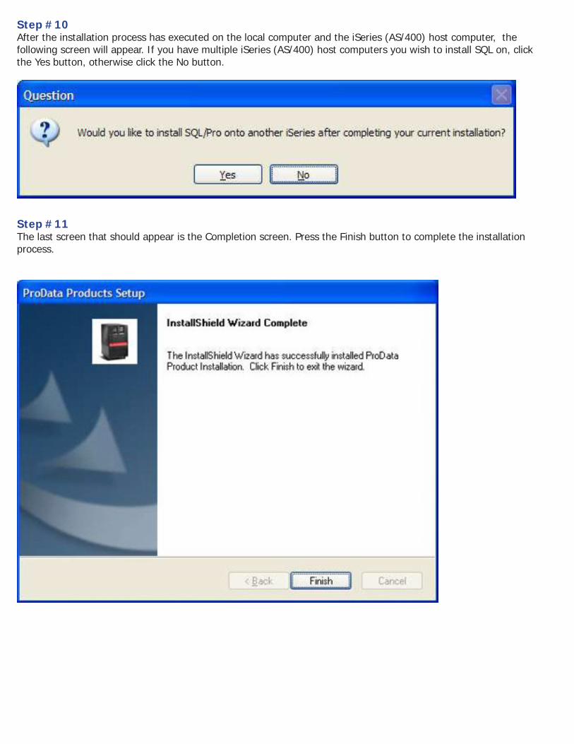
After the installation process has executed on the local computer and the iSeries (AS/400) host computer, the following screen will appear. If you have multiple iSeries (AS/400) host computers you wish to install SQL on, click the Yes button, otherwise click the No button.

Step #11 The last screen that should appear is the Completion screen. Press the Finish button to complete the installation process.

UNIT 1

What Is SQL/PRO Structured Query Language (SQL) is a powerful query language that now is supported on virtually every computer made. SQL/PRO brings the power of SQL to your AS/400 for the lowest cost. SQL provides users - both technical and non-technical - with a simple English-like language that gives them the power to query, print and manipulate any data. You’ll be able to select, organize and summarize your information in nearly any way you can imagine - certainly any way you’ll ever require! You’ll be able to direct your output to the screen, printer or database file. And programmers will appreciate the power of SQL to update files. How easy is SQL to run? The following statement will alphabetically list all records of the CUSTMAST file where state equals California:

SELECT * FROM CUSTMAST WHERE STATE=’CA’ ORDER BY STATE

What could be simpler? Our SQL/PRO interface provides truly easy-to use screens that will have you accessing the power of SQL in no time. But don’t let the ease-of-us (or the low price) fool you - SQL/PRO is powerful! With field name selection, unlimited history, our unique Saved Queries feature, submission to batch and comprehensive services, SQL/PRO is a mighty tool. You’ll find this manual not only instructs you on the workings of SQL/PRO, but it also includes very complete instructions on the writing of SQL statements themselves.

SQL Statement Entry The heart of SQL/PRO is the interactive SQL statement entry screen, where you key in any SQL statement you wish to run. The insert, split, copy, delete and split functions make it easy to enter statements. You’ll have a full 2,720 characters (34 lines by 80) to run your SQL statement. Once the statement is entered you can run it interactively or in batch from this screen.

File Field Name Selection SQL statements require that you specify the names of fields with which you will be working. With SQL/PRO there’s no need to remember field names; just press a function key and you can display the field listing of any file on your system. From this screen, you can select fields to be automatically inserted into your statement.

Report Formatting

When output is directed to a printer SQL does very little in way of report formatting. However, SQL/PRO offers you comprehensive report formatting by creating what is know to QS/400 as a Query Management form (*QMFORM) object. Report formatting criteria is submitted through a series of prompt screens that are automatically linked to your current SQL SELECT statement. The objects created by SQL/PRO are the same objects used by IBM’s SQL/400 Query Manager so, if you ever decide to purchase IBM’s SQL/400, all your queries are immediately usable by the IBM product.

History

SQL/PRO remembers every statement you run for as long as you desire. You can browse through the history to look for previous statements and rerun them. The browsing display shows the first 65 characters of the statement. From

there, you can select to retrieve the entire SQL statement to optionally modify and re-run. At any time you can purge the history field down to any number of entries.

Saved Queries

The Save Queries feature is unique to SQL/PRO. You can name and save any SQL statement you have written. Public access can be indicated for any saved queries making it easy to narrow the users that can use, change or delete query. Queries can be saved directly from the interactive entry screen or indirectly through the history screen. Once saved, you can select and run a Saved Query from the Work With Saved Queries screen interactively or via a job queue. The screen shows all the saved queries alphabetically ordered in a subfile. A special command also lets you run a saved query from a CL program.

Embed SQL in CL A SQL/PRO command lets you embed SQL statements in CL, something IBM’s Sql/400 won’t allow. You can run any SQL statement or an already-created Saved Query from a CL program. Parameters allow full control of the outfile selections. Think about how much easier this is than writing cryptic OPNQRYF commands.

UNIT 2

Using SQL/PRO

Starting SQL/PRO

Make sure that you have added the library SQLPRO to your library list. To start SQL/PRO, enter STRPDSQL at the command line.

Entering SQL Statements

The following statement entry panel will be displayed once you start SQL/PRO. From here you will enter your SQL statements.

Figure 2.1

As you can see from the panel’s lower lines, you can access all of the other functions of SQL/PRO by pressing the appropriate function keys. The cursor is initially located at the first position of the SQL statement entry field. This is where you key your SQL statement. You are allotted up to 2,720 characters (34 lines) for our SQL statement. The Page Up and Page Down keys will roll you through all 234 lines. Four function keys assist you in putting together your SQL statement. The F6 key will insert a blank line at the position of the cursor. F14 will delete the line on which the cursor is placed. F10 will copy a line to the line below it (moving down other lower lines if they contain any data). F15 will split a line at the cursor; the remainder of the line following the cursor will be moved down one line. There is no need to memorize or write down the field names of files that you will be using in an SQL statement. The F17 key will allow you to view and then insert the field names from any file. It starts by prompting you for the name of the file and the library in which it’s found. It then displays a list of the field names, sizes and field descriptions:

Figure 2.2

From here, you can select any fields to be included into your SQL statement by placing a ‘1’ to the left of the field name. Selected field names will be placed at the cursor on the SQL statement entry screen. If more than one field is selected, the fields will be separated by commas. If the statement string goes beyond the 80-column screen width, the line will automatically wrap.

Note: If you use IDDU to create your physical files, the files must be externally described or you will not be able to use them properly with SQL/PRO.

Running the SQL statement

Selecting the Output Device

You have the ability to select an output device of either display, printer or database file. This is performed by selecting option 1 from the Services menu (F13). You’ll be presented a panel that provides for the selection:

Figure 2.3 Enter the number of the selection you wish. The default output device is display. Each time you start SQL/PRO, it will begin with this setting. If you select number 3, Database file, you’ll be presented with the additional panel to define your file criteria:

Figure 2.4

When output is directed to the printer, SQL/PRO uses the print file QPQXPRTF. The default page width is 80 columns. This can be changed to 132 by enter the CHGPRTF command and specifying 132 on the Page Size keyword (width- positions per line).

Selecting the Execution Environment

You are able to run your SQL statement either interactively or in batch, depending upon how you have set it. To set the execution environment, take option 2 of the Service menu (F13). Enter a “B” for batch or “I” for interactive. The default is Interactive: each time you start SQL/PRO, it will begin with this setting.

Figure 2.5

History SQL/PRO has the ability to retain a history of executed SQL statements with the only size limitation being the capacity of your disk. Each time you hit enter to execute an SQL statement from the interactive SQL/PRO screen, the statement is logged into the SQL/PRO history file. This holds true even if the statement fails, as long as you hit enter, the statement is logged. If you key a statement and hit F22 to go into the report formatter but do not actually hit enter, the statement will not be logged. You can review the history by selecting option 5 of the Services Menu (F13). This will give you a summary listing of SQL/PRO statements, with each line showing the SQL statement and the date and time it was run. This display is in chronological order with the initial display showing the most recent page of statements. You can page back and forth through the statements with the roll keys.

Figure 2.6 You can pull up the entire SQL statement by entering a ‘1’ in the option field. A selected statement will be displayed in the original main screen. From here, you can do anything that you are able to do from the main SQL statement entry screen. You can retain as much or as little history as you like. The history file will continue to grow until you run the purge history step from the services menu. ON this step you tell it the number of statements you wish to end up with after the purge.

Saved Queries

A unique feature of SQL/PRO is Saved Queries. This function allows you to name and save any SQL statement that you have successfully run. You’ll find this invaluable for those queries that you run time and time again. Rather than rewrite the SQL statement each time, just pull up the tried and true query. For example, if you frequently run a list of all customers with a balance due, just develop it once and create a Saved Query entry with a meaningful name like BALDUE. From that point on, you only need to select and run BALDUE from the Work With Saved Queries display. In fact, you can even reference the Saved Query in a CL program with the RUNSQLSQ command (more on that later). You can create a Saved Query from any SQL statement you have on the SQL/PRO Statement Entry screen. Go to the Services menu (F13) and select option 3 (Create Saved Query). From here you will get the following panel:

Figure 2.7

Enter the name of the Saved Query (Choose an appropriate name since the list of Saved Queries displays in alphabetical order), a library and a meaningful description. The library defaults to the library specified in your configuration. Then enter the public authority which can be *ALL, *CHANGE, *USE or *EXCLUDE. This parameter default value is part of your configuration. For each of the operations listed, the public requires the corresponding authorities:

» Select or execute a saved query: *USE

» Copy or replace a saved query: *CHANGE

» Delete a saved query: *ALL

If the public is excluded from a saved query it will not be included in the list of saved queries presented by the Work With Saved Queries panel. You can save an existing saved query by specifying ‘Y’ value for Replace. The default is no (‘N’) which will cause an error message if you attempt to save a query under a name that already exists. The current output device information, including any specific database information, will be saved with the Saved Query. If you desire an output device other than the current one, you can change this. Later, when you run a Saved Query, you will be able to override the set output device if necessary. When you save a query a Query Management (*QMQRY) object is created. If you have created a report format, a Query Management Form (*QMFORM) object is also created. This can take several minutes. The save process can be submitted to batch or run interactively by specifying Y or N in the submit to batch parameter. A default value of Y or N can be stored by using the configuration service option from the Services panel. You may wish to create a Saved Query from a statement in your history. To do this, select the statement from the history display to bring it up in the SQL/PRO Statement Entry screen. Then proceed as discussed above as if you had just keyed it. Now to view the Saved Queries, select option 4 (Work With Saved Queries) from the Services menu (F13). Here is a sample of the Work With Saved Queries screen:

Figure 2.8

From here you can run a job, select it, delete it, copy it or print the statement by entering the appropriate number in the option field to the left of the query name. Queries can be saved to libraries of your choice therefore the “Work with Saved Queries” panel allows you to choose the library from which to display saved queries. The library defaults to the target library that has been configured by the user from the Configuration function panel. With the WRKSQ command you can directly access the “Work with Saved Queries” display for saved queries within the library you specify. The format is:

WRKSQ LIB (library_name) All options will be available except Select therefore, you cannot edit a saved query from the WRKSQ command.

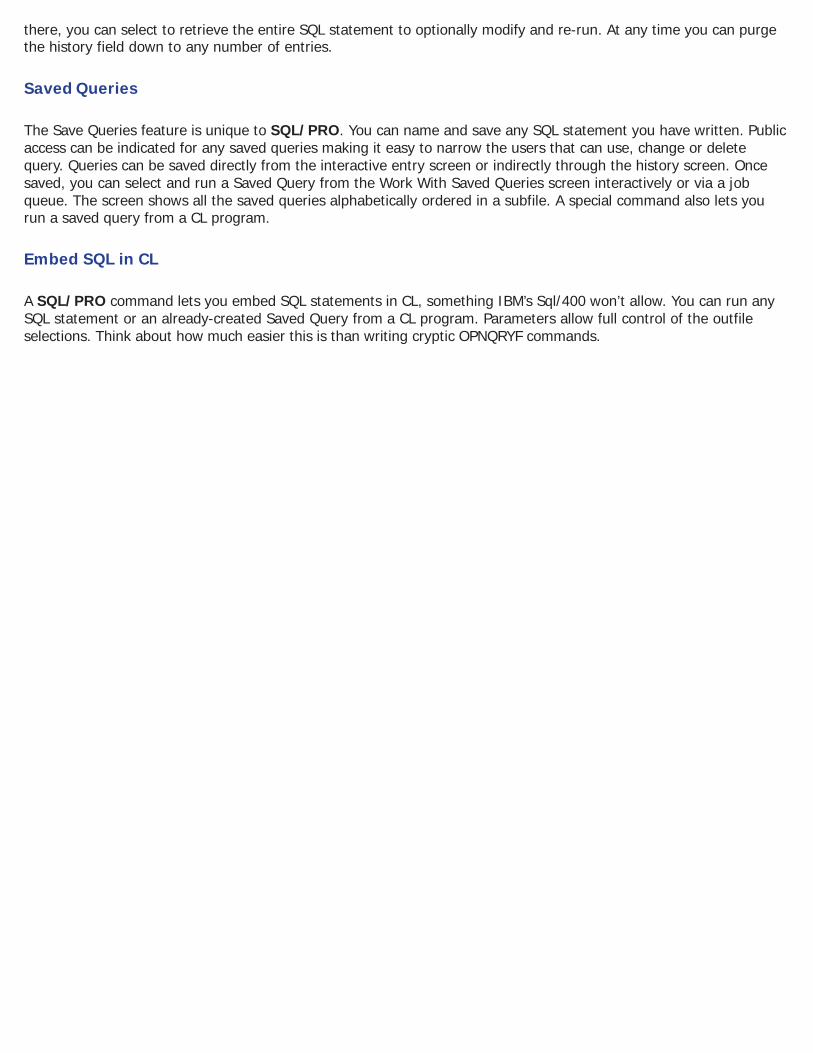
Running a Saved Query You can run a saved query either in batch or interactively. Option 9 runs it interactively and 8 runs it in batch. You can also run a Saved Query by selecting it with option 1 which will copy it into the SQL Statement Entry Screen. Then follow the normal run procedures from there. With either of these three methods, you can run the job using the output device stored in the Saved Query, unless you choose to override the output device on the following screen (which is presented automatically prior to execution):

Figure 2.9

Changing the output parameters will only affect running this current statement. Once completed, the session values that were in effect prior to selecting the Saved Query will be in effect once again. You can also override any value of a Saved Query by selecting it with option 1 and then changing the statement itself, the output device and the execution environment before running the statement.

Changing a Saved Query Changing a Saved Query begins the same as overriding a Saved Query. You select with option 1 to bring the statement into the SQL Statement Entry screen. Make any changes to the statement you want. Then, go to the Services menu and run option 3 to save the query. You will be presented with the name of the query, the description, the public or private authorization and the output device that you specified when you last saved this query. At this point you can change any value before pressing enter. Obviously if you are changing a Saved Query, keep the Query name the same. However, you can change the name to save the query to a new Saved Query name.

Copying a Saved Query The easiest way to copy a Saved Query is with option 3. This will provide you with the following screen from which you can copy to another Saved Query of another name.

Figure 2.10

Deleting a Saved Query

You can delete a Saved Query with option 4. You will be presented with a screen to confirm the deletion. You can also use the DLTSQ command described later in this section.

Printing a Saved Query

You can print a Saved Query with option 6.

Services

In previous sections of this chapter we’ve pointed you to the Services menu. This is it:

Figure 2.11

You’ve already seen how you can select the output device, set the execution options, work with history and create and work with Saved Queries. Option 6, Work with History, allows you to reorganize your history file. SQL/PRO stores history records for each user in a separate member of the history file. Eventually you will want to reorganize your history file to remove old, unwanted entries.

Running a Save Query from the Command Line The command STRQMQRY will allow you to run a Saved Query from the command line. By keying STRQMQRY and pressing F4, you’ll get this panel:

Figure 2.12

Figure 2.13

In this example we are running the Saved Query LSTCSTMST, printing the output and substituting the value ‘AZ’ for the variable STATE. (Refer to chapter 5 for more information about variables.) Just key the name of the Saved Query and any other necessary information and press enter. This will begin running the Saved query as it is set up with SQL/PRO.

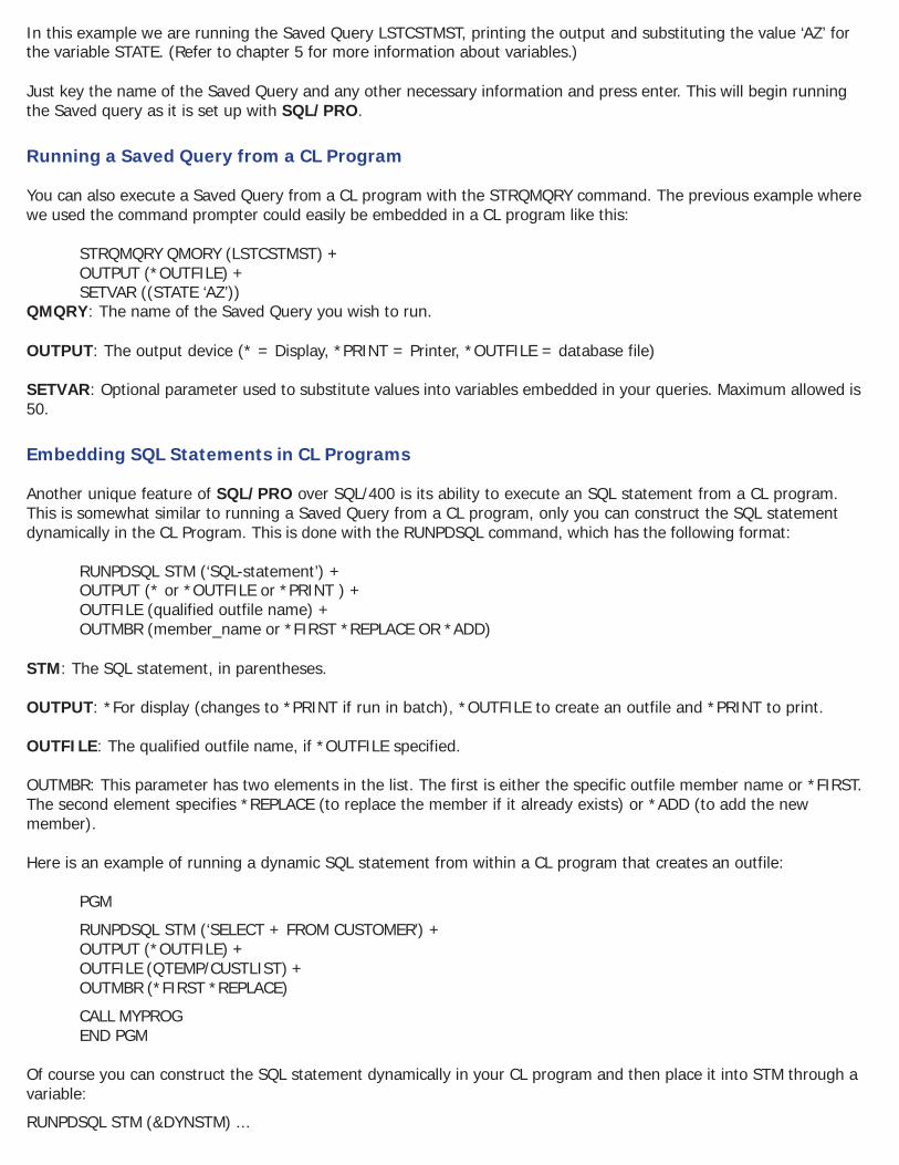
Running a Saved Query from a CL Program You can also execute a Saved Query from a CL program with the STRQMQRY command. The previous example where we used the command prompter could easily be embedded in a CL program like this:

STRQMQRY QMORY (LSTCSTMST) + OUTPUT (*OUTFILE) + SETVAR ((STATE ‘AZ’))

QMQRY: The name of the Saved Query you wish to run. OUTPUT: The output device (* = Display, *PRINT = Printer, *OUTFILE = database file) SETVAR: Optional parameter used to substitute values into variables embedded in your queries. Maximum allowed is 50.

Embedding SQL Statements in CL Programs Another unique feature of SQL/PRO over SQL/400 is its ability to execute an SQL statement from a CL program. This is somewhat similar to running a Saved Query from a CL program, only you can construct the SQL statement dynamically in the CL Program. This is done with the RUNPDSQL command, which has the following format:

RUNPDSQL STM (‘SQL-statement’) + OUTPUT (* or *OUTFILE or *PRINT ) + OUTFILE (qualified outfile name) + OUTMBR (member_name or *FIRST *REPLACE OR *ADD)

STM: The SQL statement, in parentheses. OUTPUT: *For display (changes to *PRINT if run in batch), *OUTFILE to create an outfile and *PRINT to print. OUTFILE: The qualified outfile name, if *OUTFILE specified. OUTMBR: This parameter has two elements in the list. The first is either the specific outfile member name or *FIRST. The second element specifies *REPLACE (to replace the member if it already exists) or *ADD (to add the new member). Here is an example of running a dynamic SQL statement from within a CL program that creates an outfile:

PGM

RUNPDSQL STM (‘SELECT + FROM CUSTOMER’) + OUTPUT (*OUTFILE) + OUTFILE (QTEMP/CUSTLIST) + OUTMBR (*FIRST *REPLACE)

CALL MYPROG END PGM

Of course you can construct the SQL statement dynamically in your CL program and then place it into STM through a variable:

RUNPDSQL STM (&DYNSTM) ...

Retrieving a Saved Query into a Variable

You may have a reason to retrieve a Saved Query statement into a variable. For example, you may want to retrieve one, modify it in a CL program, and then run the modified statement with our RUNPDSQL command. You can do this with the RTVSQLSQ command:

Figure 2.14

Converting Query/400 Queries to SQL/PRO

For those of you who have Query/400 queries SQL/PRO provides the Convert QRYDFN to SQL/PRO (CVTQRYSQL) command which will convert any QUERY/400 query to an SQL/PRO saved query. The converted query will execute through SQL/PRO just as it did through QUERY/400. However, if you need to edit the report format, the report formatter will force you to create your report format from scratch.

Figure 2.15

Unit 3

Writing SQL/PRO Statements

NOTE: This chapter explains using the most common features of SQL’s data manipulation statements. Since SQL/PRO is ANSI compatible (uses industry-accepted standards), you can pick up any inexpensive SQL book form your local bookstore to gain more in-depth education about all the features and statements of SQL.

SQL on the AS/400 is a full function database language. With it you can create a database as well as manipulate the data it contains. You can also access an already existing database. For the purpose of this product we will only concentrate on those statements that allow you to manipulate an existing database. There are other books available which can teach you the full range of SQL. Each of the data manipulation statements will be explained and information regarding restrictions and rules will be provided. It is not necessary to fully comprehend each rule before attempting to use the statements. However, we are providing the information here as a reference. You will find that the more you use SQL, the better your comprehension of it will become. Do not become discouraged if you don’t fully understand each topic. Just try using the statements, and the meanings will become clearer. Most of the limits set by SQL are at such an extreme, that most AS/400 shops will never encounter them. Also, for practical purposes, you probably would not want to reach the level of complexity that would exceed those limits. We will now start our discussion of the data manipulation language statements that are available within SQL/400.

The COMMENT ON Statement The COMMENT ON statement adds or replaces comments in the catalog descriptions of tables, views packages (programs) or columns.The syntax for the COMMENT ON statement is as follows:

COMMENT ON <TABLE> <TABLE NAME or VIEW NAME> IS <STRING CONSTANT> <COLUMN> <TABLE NAME or VIEW NAME/COLUMN NAME> <PACKAGE> <PACKAGE NAME>

Example:

COMMENT ON TABLE CUSTMAST IS ‘TEST FILE’

The CREATE COLLECTION Statement The CREATE COLLECTION statement defines a collection in which tables, views and indexes can be created. A collection is created as one of the following: A library (relates objects and allows you to find them by name), A catalog (contains descriptions and consists of a data dictionary and a set of views and logical files) or A Journal and journal receiver (a journal QSQJRN and journal receiver QSQJRN0001 is created in the collection and records changes to all tables created in the collection). This syntax for the CREATE COLLECTION statement is as follows:

CREATE COLLECTION

The CREATE INDEX Statement The CREATE INDEX statement creates an index on a table.

The syntax for the CREATE INDEX statement is as follows:

CREATE [UNIQUE OR WHERE NOT NULL] INDEX <INDEX NAME> ON <TABLE NAME> (<COLUMN NAME> [ASC OR DESC])

The CREATE TABLE Statement The CREATE TABLE statement allows you to create a table (i.e., physical file) and define the physical attributes of the columns in the table. When this statement is executed, a new, empty table is created with the column information as defined. The first parameter specifies the column name, the second parameter specifies the data type and length for that column and the third parameter specifies if the column can be null.

The syntax for the CREATE TABLE statement is as follows:

CREATE TABLE <TABLE NAME> (<COLUMN NAME> <DATA TYPE>[(LENGTH)] [NOT NULL OR NOT NULL WITH DEFAULT]

Example:

CREATE TABLE CUSTMAST (CUSTNUM NUMERIC (8) NOT NULL, CUSTNAM CHAR (28) NOT NULL, ADDR1 CHAR (38) NOT NULL, ADDR2 CHAR (38) , SLSAMT DECIMAL (8, 2))

The CREATE VIEW Statement The CREATE VIEW statement will create a subset of a file or table. Creating a view is very much like creating a table, in so much as you must define the attributes of the columns. You must have at least one of the following authorities over the table or file in order to create a view of it: SELECT, UPDATE, INSERT or DELETE. If you do not specify column names in the view, then the names are the same as those in the table or file you are creating the view from. Since the view is totally dependent on one or more tables or files for data, it has no data of its own, therefore it requires no storage for the data. Consequently when you update the data in a view, you are actually updating the data in the table or file.

The syntax for the CREATE VIEW statement is as follows:

CREATE VIEW <VIEW NAME> [(COLUMN NAME)] AS <SUBSELECT>

Example:

CREATE VIEW CUSTLIST (CUSTNUM, CUSTNAM) AS SELECT CUSTNUM, CUSTNAM FROM CUSTMAST WHERE CUST NUM > 20000001

The DROP Statement The DROP statement deletes an object. Any object that is directly or indirectly dependent on that object is also deleted. The syntax for the DROP statement is as follows:

DROP <COLLECTION> <COLLECTION NAME> <INDEX> <INDEX NAME> <TABLE> <TABLE NAME> <VIEW> <VIEW NAME> <PACKAGE> <PACKAGE NAME>

The GRANT Statement The GRANT statement grants the privilege to execute statements in a package.

The syntax for the GRANT statement is as follows:

GRANT EXECUTE ON PACKAGE <PACKAGE NAME> TO <AUTHORIZATION NAME>

The LABEL ON Statement The LABEL ON statement adds or replaces labels in the catalog descriptions of tables, views, packages or columns.

The syntax for the LABEL ON statement is as follows:

LABEL ON <TABLE> <TABLE NAME> IS <STRING CONSTANT> <COLUMN> <COLUMN NAME> <VIEW> <VIEW NAME> <PACKAGE> <PACKAGE NAME>

The LOCK TABLE Statement The LOCK TABLE statement acquires a shared or exclusive lock on a specified table. The share mode prevents any concurrent application processes to be executed on the table with the exception of read only operations. The exclusive mode prevents any concurrent operations at all to be executed on the table. The syntax for the LOCK TABLE statement is as follows:

LOCK TABLE <TABLE NAME> IN <SHARE OR EXCLUSIVE> MODE

The REVOKE Statement The Revoke statement removes privileges on a table or view. It can remove all privileges or one or more of the following privileges: SELECT, DELETE, INDEX, INSERT or UPDATE. The syntax for the REVOKE statement is as follows:

REVOKE <PRIVILEGES> ON <TABLE NAME> FROM <AUTHORIZATION NAME> [<ALL>] <VIEW NAME>

The SELECT Statement The SELECT statement allows you to read or list records from a file or files. You can condition how records are selected, sort the resulting table, perform group summary operations and join files together.

The syntax for the SELECT statement is as follows:

SELECT [DISTINCT | ALL <value expression>,... FROM {<library/file>} [<alias>,...

[WHERE <predicate>] [GROUP BY {<field name>,...}] [HAVING <predicate>] [UNION | ALL] [ORDER BY {<field name> | <relative field position>},...]

The clauses above are listed in the order in which they can be used. You are not required to use any of these, except the SELECT and FROM clauses. However, if you do use any, they must be in the order listed.

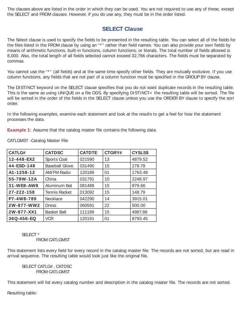
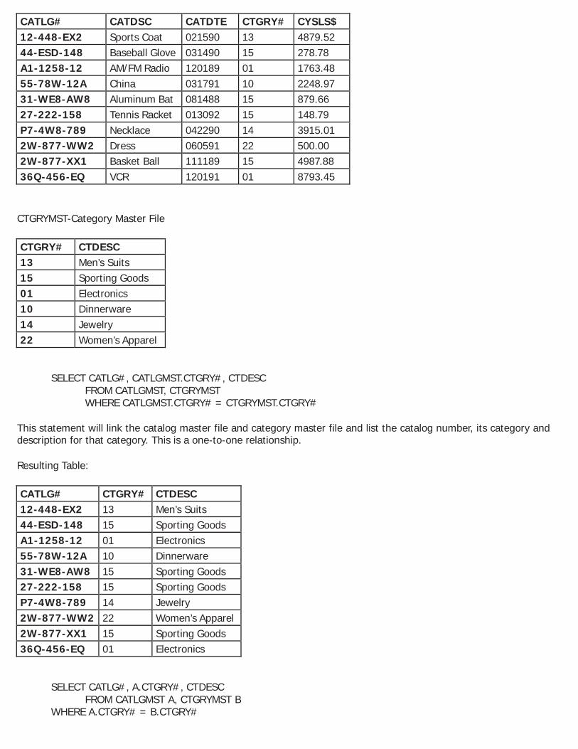
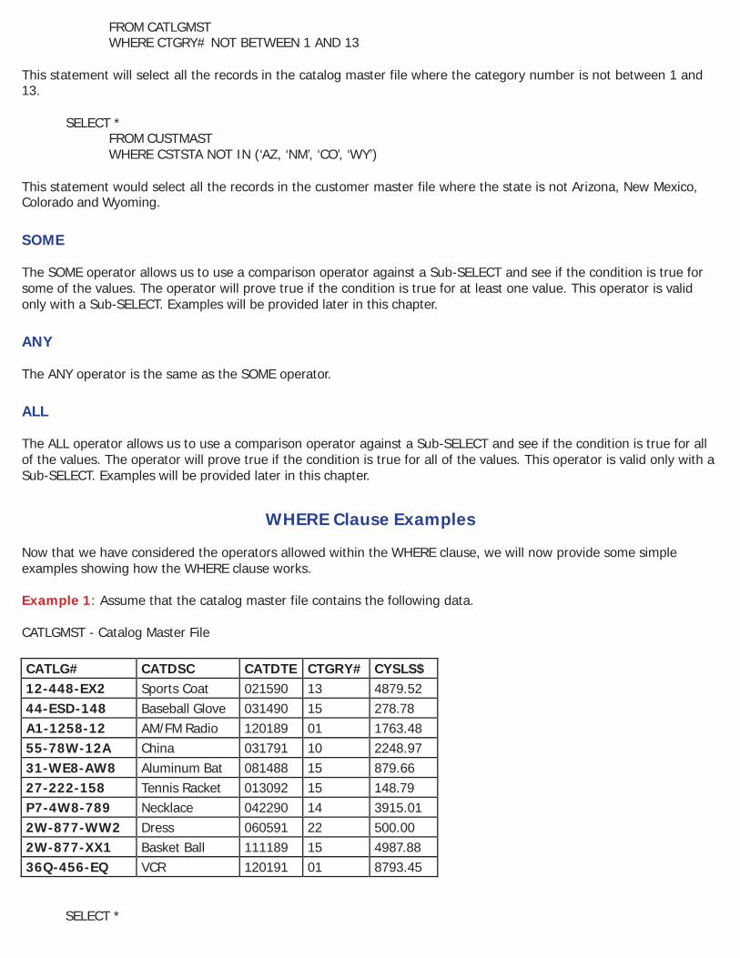
SELECT Clause The Select clause is used to specify the fields to be presented in the resulting table. You can select all of the fields for the files listed in the FROM clause by using an “*” rather than field names. You can also provide your own fields by means of arithmetic functions, built-in functions, column functions, or literals. The total number of fields allowed is 8,000. Also, the total length of all fields selected cannot exceed 32,766 characters. The fields must be separated by commas. You cannot use the “*” (all fields) and at the same time specify other fields. They are mutually exclusive. If you use column functions, any fields that are not part of a column function must be specified in the GROUP BY clause. The DISTINCT keyword on the SELECT clause specifies that you do not want duplicate records in the resulting table. This is the same as using UNIQUE on a file DDS. By specifying DISTINCT< the resulting table will be sorted. The file will be sorted in the order of the fields in the SELECT clause unless you use the ORDER BY clause to specify the sort order. In the following examples, examine each statement and look at the results to get a feel for how the statement processes the data. Example 1: Assume that the catalog master file contains the following data. CATLGMST -Catalog Master File

CATLG# CATDSC CATDTE CTGRY# CYSLS$ 12-448-EX2 Sports Coat 021590 13 4879.52 44-ESD-148 Baseball Glove 031490 15 278.78 A1-1258-12 AM/FM Radio 120189 01 1763.48 55-78W-12A China 031791 10 2248.97 31-WE8-AW8 Aluminum Bat 081488 15 879.66 27-222-158 Tennis Racket 013092 15 148.79 P7-4W8-789 Necklace 042290 14 3915.01 2W-877-WW2 Dress 060591 22 500.00 2W-877-XX1 Basket Ball 111189 15 4987.88 36Q-456-EQ VCR 120191 01 8793.45

SELECT * FROM CATLGMST

This statement lists every field for every record in the catalog master file. The records are not sorted, but are read in arrival sequence. The resulting table would look just like the original file.

SELECT CATLG#, CATDSC FROM CATLGMST

This statement will list every catalog number and description in the catalog master file. The records are not sorted. Resulting table:

CATLG# CATDSC 12-448-EX2 Sports Coat 44-ESD-148 Baseball Glove A1-1258-12 AM/FM Radio 55-78W-12A China 31-WE8-AW8 Aluminum Bat 27-222-158 Tennis Racket P7-4W8-789 Necklace 2W-877-WW2 Dress 2W-877-XX1 Basket Ball 36Q-456-EQ VCR

SELECT *, CYSLS$+LYSLS$ FROM CATLGMST

This statement is invalid since the “*” is used with field names in the SELECT clause.

Example 2: Assume that the catalog master file contains the following data. CATLGMST-

Catalog Master File

CATLG# CYSLS$ LYSLS$ 12-448-EX2 4879.52 7894.22 44-ESD-148 278.78 1489.77 A1-1258-12 1763.48 1589.44 55-78W-12A 2248.97 789.88 31-WE8-AW8 879.66 444.48 27-222-158 148.79 0.00 P7-4W8-789 3915.01 3879.11 2W-877-WW2 550.00 2489.45 2W-877-XX1 4987.88 7265.37 36Q-456-EQ 8793.45 4276.40

SELECT CATLG#, ‘Total Sales:’, CYSLS$+LYSLS$ FROM CATLGMST

This statement will list each catalog number in the catalog master file and the sum of the current sales and last year’s sales. Also, a literal of ‘Total Sales:’ will be listed for each catalog number. Resulting Table:

CATLG# CYSLS$+LYSLS$ 12-448-EX2 Total Sales: 12773.74 44-ESD-148 Total Sales: 1768.55 A1-1258-12 Total Sales: 3352.92 55-78W-12A Total Sales: 3038.85 31-WE8-AW8 Total Sales: 1324.14 27-222-158 Total Sales: 148.79 P7-4W8-789 Total Sales: 7794.12 2W-877-WW2 Total Sales: 2989.45 2W-877-XX1 Total Sales: 12253.25 36Q-456-EQ Total Sales: 13069.85

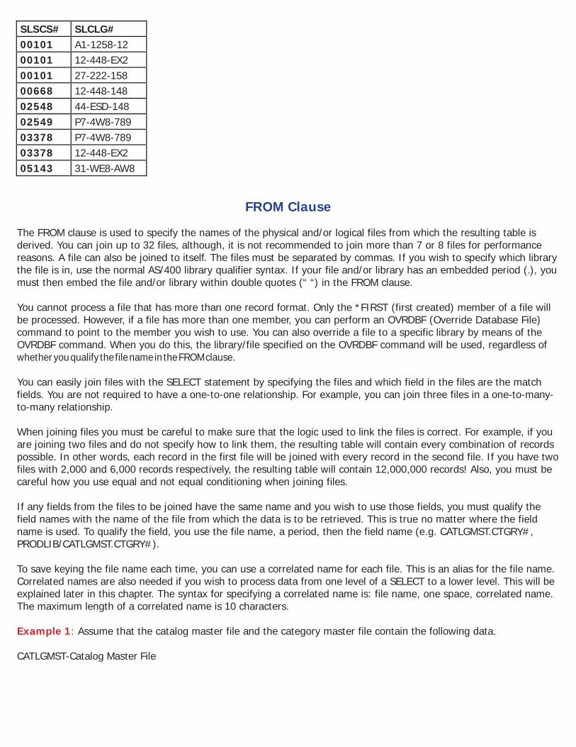
Example 3: Assume that the sales history file contains the following data: SALESHST-Sales History File

SLSO# SLSCS# SLCLG# 13478 00101 12-448-EX2 15897 02548 44-ESD-148 13478 00101 A1-1258-12 12489 03378 12-448-EX2 11457 02143 31-WE8-AW8 14999 00101 27-222-158 16678 03378 P7-4W8-789 14875 00668 12-448-148 15155 02549 P7-4WS-789 17891 02548 44-ESD-148

SELECT DISTINCT SLSCS#, SLCLG# FROM SALESHST

This statement will list every unique occurrence of the customer number and catalog number in the sales history file. The resulting table will be sorted in the order of SLSCS# and SLCLG. Notice that order numbers 15897and 17891 produced only one record in the table. This is because the customer and catalog numbers were the same. Resulting Table:

SLSCS# SLCLG# 00101 A1-1258-12 00101 12-448-EX2 00101 27-222-158 00668 12-448-148 02548 44-ESD-148 02549 P7-4W8-789 03378 P7-4W8-789 03378 12-448-EX2 05143 31-WE8-AW8

FROM Clause The FROM clause is used to specify the names of the physical and/or logical files from which the resulting table is derived. You can join up to 32 files, although, it is not recommended to join more than 7 or 8 files for performance reasons. A file can also be joined to itself. The files must be separated by commas. If you wish to specify which library the file is in, use the normal AS/400 library qualifier syntax. If your file and/or library has an embedded period (.), you must then embed the file and/or library within double quotes (“ “) in the FROM clause. You cannot process a file that has more than one record format. Only the *FIRST (first created) member of a file will be processed. However, if a file has more than one member, you can perform an OVRDBF (Override Database File) command to point to the member you wish to use. You can also override a file to a specific library by means of the OVRDBF command. When you do this, the library/file specified on the OVRDBF command will be used, regardless of whether you qualify the file name in the FROM clause. You can easily join files with the SELECT statement by specifying the files and which field in the files are the match fields. You are not required to have a one-to-one relationship. For example, you can join three files in a one-to-many- to-many relationship. When joining files you must be careful to make sure that the logic used to link the files is correct. For example, if you are joining two files and do not specify how to link them, the resulting table will contain every combination of records possible. In other words, each record in the first file will be joined with every record in the second file. If you have two files with 2,000 and 6,000 records respectively, the resulting table will contain 12,000,000 records! Also, you must be careful how you use equal and not equal conditioning when joining files. If any fields from the files to be joined have the same name and you wish to use those fields, you must qualify the field names with the name of the file from which the data is to be retrieved. This is true no matter where the field name is used. To qualify the field, you use the file name, a period, then the field name (e.g. CATLGMST.CTGRY#, PRODLIB/CATLGMST.CTGRY#). To save keying the file name each time, you can use a correlated name for each file. This is an alias for the file name. Correlated names are also needed if you wish to process data from one level of a SELECT to a lower level. This will be explained later in this chapter. The syntax for specifying a correlated name is: file name, one space, correlated name. The maximum length of a correlated name is 10 characters. Example 1: Assume that the catalog master file and the category master file contain the following data. CATLGMST-Catalog Master File


CTGRYMST-Category Master File

CTGRY# CTDESC 13 Men’s Suits 15 Sporting Goods 01 Electronics 10 Dinnerware 14 Jewelry 22 Women’s Apparel

SELECT CATLG#, CATLGMST.CTGRY#, CTDESC FROM CATLGMST, CTGRYMST WHERE CATLGMST.CTGRY# = CTGRYMST.CTGRY#

This statement will link the catalog master file and category master file and list the catalog number, its category and description for that category. This is a one-to-one relationship. Resulting Table:

CATLG# CTGRY# CTDESC 12-448-EX2 13 Men’s Suits 44-ESD-148 15 Sporting Goods A1-1258-12 01 Electronics 55-78W-12A 10 Dinnerware 31-WE8-AW8 15 Sporting Goods 27-222-158 15 Sporting Goods P7-4W8-789 14 Jewelry 2W-877-WW2 22 Women’s Apparel 2W-877-XX1 15 Sporting Goods 36Q-456-EQ 01 Electronics

SELECT CATLG#, A.CTGRY#, CTDESC FROM CATLGMST A, CTGRYMST B

WHERE A.CTGRY# = B.CTGRY#

This statement is the same as the previous example, but this one uses a correlated name instead of the file names. As you can see, this would be much easier to work with. Example 2: Assume that the order header and order item files contain the following data. ORDERHDR-Order Header File

OHORD# OHCST# 13478 00101 15897 02548 12489 03378 11457 05143 14999 00101 16678 03378 14875 00668 15155 02549 17891 02548

ORDERITM-Order Item File

OHORD# OICLG# OIOQTY OISQTY 13478 12-448-EX 200 195 15897 44-ESD-148 22 22 13478 A1-1258-12 134 144 12489 12-448-EX2 300 300 11457 31-WE8-AW8 15 0 14999 27-222-158 36 36 16678 P7-4W8-789 19 0 14875 12-448-148 87 87 15155 P7-4W8-789 112 0 17891 44-ESD-148 2145 0

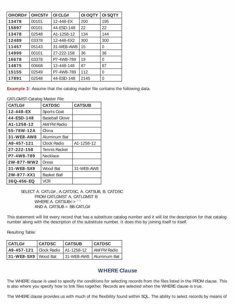
SELECT OHORD#, OHCST#, OICLG#, OIOQTY, OISQTY FROM ORDERHDR, ORDERITM

WHERE OHORD# = OIORD# This statement will link each record in the order header file to each record in the order item file where the order numbers are the same. This is a one-to-many relationship. Resulting Table:

OHORD# OHCST# OICLG# OIOQTY OISQTY 13478 00101 12-448-EX 200 195 15897 00101 44-ESD-148 22 22 13478 02548 A1-1258-12 134 144 12489 03378 12-448-EX2 300 300 11457 05143 31-WE8-AW8 15 0 14999 00101 27-222-158 36 36 16678 03378 P7-4W8-789 19 0 14875 00668 12-448-148 87 87 15155 02549 P7-4W8-789 112 0 17891 02548 44-ESD-148 2145 0

Example 3: Assume that the catalog master file contains the following data. CATLGMST-Catalog Master File

CATLG# CATDSC CATSUB 12-448-EX Sports Coat

44-ESD-148 Baseball Glove

A1-1258-12 AM/FM Radio

55-78W-12A China

31-WE8-AW8 Aluminum Bat

A9-457-121 Clock Radio A1-1258-12 27-222-158 Tennis Racket

P7-4W8-789 Necklace

2W-877-WW2 Dress

31-WE8-SX9 Wood Bat 31-WE8-AW8 2W-877-XX1 Basket Ball

36Q-456-EQ VCR

SELECT A. CATLG#, A.CATDSC, A. CATSUB, B. CATDSC FROM CATLGMST A, CATLGMST B WHERE A. CATSUB<> ‘ ‘ AND A. CATSUB = BB.CATLG#

This statement will list every record that has a substitute catalog number and it will list the description for that catalog number along with the description of the substitute number. It does this by joining itself to itself. Resulting Table:

CATLG# CATDSC CATSUB CATDSC A9-457-121 Clock Radio A1-1258-12 AM/FM Radio 31-WE8-SX9 Wood Bat 31-WE8-AW8 Aluminum Bat

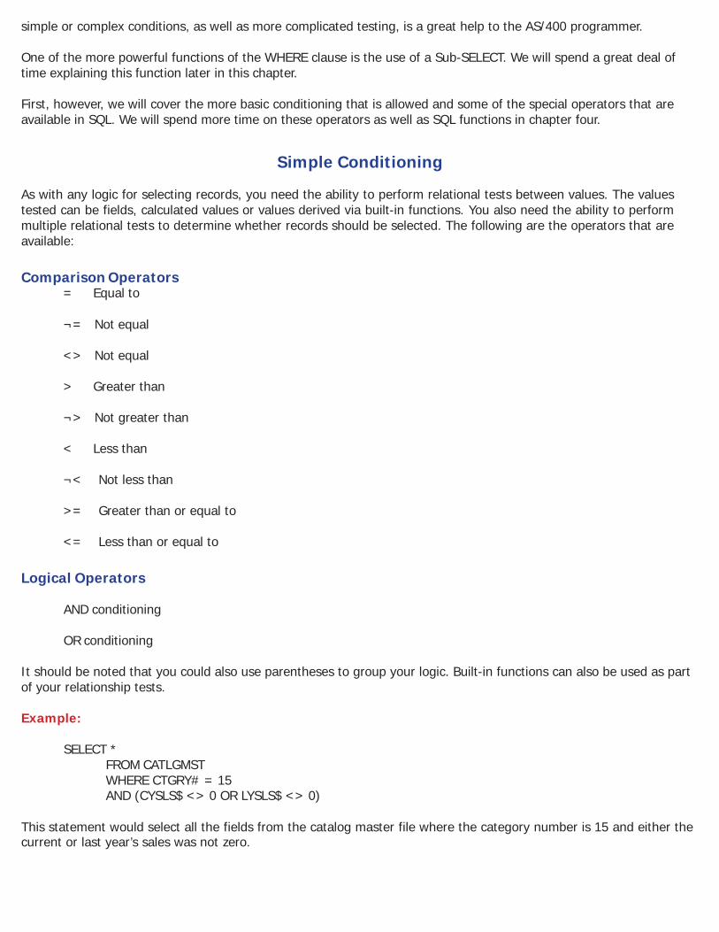
WHERE Clause The WHERE clause is used to specify the conditions for selecting records from the files listed in the FROM clause. This is also where you specify how to link files together. Records are selected when the WHERE clause is true. The WHERE clause provides us with much of the flexibility found within SQL. The ability to select records by means of

simple or complex conditions, as well as more complicated testing, is a great help to the AS/400 programmer. One of the more powerful functions of the WHERE clause is the use of a Sub-SELECT. We will spend a great deal of time explaining this function later in this chapter. First, however, we will cover the more basic conditioning that is allowed and some of the special operators that are available in SQL. We will spend more time on these operators as well as SQL functions in chapter four.

Simple Conditioning As with any logic for selecting records, you need the ability to perform relational tests between values. The values tested can be fields, calculated values or values derived via built-in functions. You also need the ability to perform multiple relational tests to determine whether records should be selected. The following are the operators that are available:

Comparison Operators = Equal to

¬= Not equal

<> Not equal

> Greater than

¬> Not greater than

< Less than

¬< Not less than

>= Greater than or equal to

<= Less than or equal to

Logical Operators

AND conditioning

OR conditioning

It should be noted that you could also use parentheses to group your logic. Built-in functions can also be used as part of your relationship tests. Example:

SELECT * FROM CATLGMST WHERE CTGRY# = 15 AND (CYSLS$ <> 0 OR LYSLS$ <> 0)

This statement would select all the fields from the catalog master file where the category number is 15 and either the current or last year’s sales was not zero.

Complex Conditioning SQL also provides some additional operators for selecting records. The following are the operators available and how they are used.

BETWEEN The BETWEEN operator allows us to test whether a value or expression is between two different values, inclusively. The syntax for the BETWEEN operator is: Value BETWEEN value AND value

The values used can be any field or a calculated value. This operator is valid for both numeric and character data.

It is up to you to insure that the range specified is valid. If the second value (after the AND) is less than the first value, no records would be selected. No error is indicated when this occurs. Examples:

SELECT * FROM CATLGMST WHERE CTGRY# BETWEEN 1 AND 13

This statement would select all the records in the catalog master file where the category number is between 1 and 13. This would be the equivalent of saying:

WHERE CTGRY# >= 1 AND CTGRY# <= 13

SELECT * FROM CUSTMAST WHERE CSTZIP BETWEEN ‘44000’ AND ‘44999’

This statement would select all the records in the customer master file where the zip code is between ‘44000’ and ‘44999.’ This would be the same as saying that the zip code begins with ‘44’. Because CSTZIP is a character field, single quotes or apostrophes are used when specifying the range.

SELECT * FROM CATLGMST WHERE LYSLS$ BETWEEN L2SLS$ AND CYSLS$

This statement would select all the records in the catalog master file where last years sales is between two years ago and the current years sales. If the field LYSLS$ is later than CYCLS$ or earlier than L2SLS$, the record would not be selected.

LIKE The LIKE operator allows us to test a string value to see if it contains certain characters. There are two special characters that you can use to specify how to look for the characters. The first special character is %, which indicates any number of missing characters. The second is , which indicates one character only. By combining the % and _, you can find any combination of characters. When using the LIKE operator there is no provision made for translating a string value. Therefore, the LIKE operator is case sensitive. The syntax for the LIKE operator is:

value LIKE ‘search characters’ Examples:

SELECT * FROM CATLGMST WHERE CATDSC LIKE ‘%Apparel%’

This statement would select all the records in the catalog master file where the description contains the word “Apparel.” There can be any number of characters prior to the word and any number of characters after the word.

SELECT * FROM CATLGMST

WHERE CATDSC LIKE ‘ _o% This statement would select all the records in the catalog master file where the second character in the description is the letter “o.”

IN The IN operator allows you to test a value to see if it exists in a list of values. The list can either be provided or can be derived from a Sub-SELECT. The Sub-SELECT will be explained a little later in this chapter. The syntax for the IN operator is: Value IN (value list or Sub-SELECT) This operator is valid for both numeric and character data. When you provide the values to be tested, they must be separated by commas. Example:

SELECT * FROM CUSTMAST WHERE CSTSTA IN (‘AZ, ‘NM’, ‘CO’, ‘WY’)

This statement would select all the records in the customer master file where the state is either Arizona, New Mexico, Colorado or Wyoming.

EXISTS The EXISTS operator will test to see if any records exist in a Sub-SELECT. If any records were selected by the Sub- SELECT, the condition is true. The syntax for the EXISTS operator is: EXISTS (Sub-SELECT) Examples will be provided later in this chapter.

NOT The NOT operator can be used in connection with the following operators: BETWEEN,IN, LIKE and EXISTS. The NOT operator performs a negative test. If the operator is true, the NOT will make it false and vice-versa. Examples:

SELECT *

SELECT *

FROM CATLGMST WHERE CTGRY# NOT BETWEEN 1 AND 13

This statement will select all the records in the catalog master file where the category number is not between 1 and 13.

SELECT * FROM CUSTMAST WHERE CSTSTA NOT IN (‘AZ, ‘NM’, ‘CO’, ‘WY’)

This statement would select all the records in the customer master file where the state is not Arizona, New Mexico, Colorado and Wyoming.

SOME The SOME operator allows us to use a comparison operator against a Sub-SELECT and see if the condition is true for some of the values. The operator will prove true if the condition is true for at least one value. This operator is valid only with a Sub-SELECT. Examples will be provided later in this chapter.

ANY The ANY operator is the same as the SOME operator.

ALL The ALL operator allows us to use a comparison operator against a Sub-SELECT and see if the condition is true for all of the values. The operator will prove true if the condition is true for all of the values. This operator is valid only with a Sub-SELECT. Examples will be provided later in this chapter.

WHERE Clause Examples Now that we have considered the operators allowed within the WHERE clause, we will now provide some simple examples showing how the WHERE clause works. Example 1: Assume that the catalog master file contains the following data. CATLGMST - Catalog Master File


FROM CATLGMST WHERE CTGRY# = 15

This will select all fields for records in the catalog master file where the catalog group number is equal to 15. Resulting Table:

CATLG# CATDSC CATDTE CTGRY# CYSLS$ 44-ESD-148 Baseball Glove 031490 15 278.78 31-WE8-AW8 Aluminum Bat 081488 15 879.66 27-222-158 Tennis Racket 013092 15 148.79 2W-877-XX1 Basket Ball 111189 15 4987.88

SELECT * FROM CATLGMST WHERE CTGRY# = 15 AND CYSLS$ > 500

This will select all fields for records in the catalog master file where the catalog group number is equal to 15 and the current year sales is greater from $500.00. Resulting Table:

CATLG# CATDSC CATDTE CTGRY# CYSLS$ 31-WE8-AW8 Aluminum Bat 081488 15 879.66 2W-877-XX1 Basket Ball 111189

15 4987.88

SELECT * FROM CATLGMST WHERE CTGRY# = 15 AND SUBSTR (CATLG#, 1,1) = ‘2’ OR CYSLS$ > 500

This will select all fields for records in the catalog master file where the catalog group number is equal to 15 and the first character of the catalog number is a “2” or if the current year sales is greater than $500.00. Resulting Table:

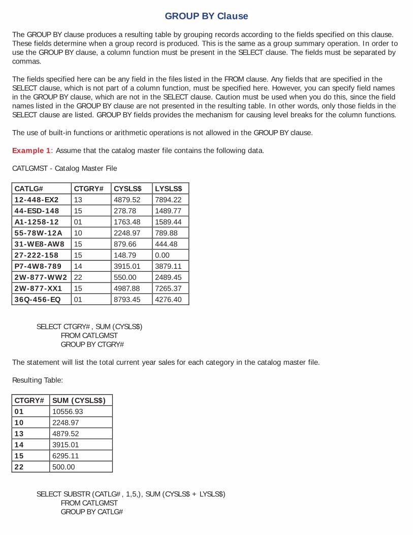
CATLG# CATDSC CATDTE CTGRY# CYSLS$ 12-448-EX2 Sports Coat 021590 13 4879.52 A1-1258-12 AM/FM Radio 120189 01 1763.48 55-78W-12A China 031791 10 2248.97 27-222-158 Tennis Racket 013092 15 148.79 P7-4W8-789 Necklace 042290 14 3915.01 2W-877-XX1 Basket Ball 111189 15 4987.88 36Q-456-EQ VCR 120191 01 8793.45

GROUP BY Clause The GROUP BY clause produces a resulting table by grouping records according to the fields specified on this clause. These fields determine when a group record is produced. This is the same as a group summary operation. In order to use the GROUP BY clause, a column function must be present in the SELECT clause. The fields must be separated by commas. The fields specified here can be any field in the files listed in the FROM clause. Any fields that are specified in the SELECT clause, which is not part of a column function, must be specified here. However, you can specify field names in the GROUP BY clause, which are not in the SELECT clause. Caution must be used when you do this, since the field names listed in the GROUP BY clause are not presented in the resulting table. In other words, only those fields in the SELECT clause are listed. GROUP BY fields provides the mechanism for causing level breaks for the column functions. The use of built-in functions or arithmetic operations is not allowed in the GROUP BY clause. Example 1: Assume that the catalog master file contains the following data. CATLGMST - Catalog Master File

CATLG# CTGRY# CYSLS$ LYSLS$ 12-448-EX2 13 4879.52 7894.22 44-ESD-148 15 278.78 1489.77 A1-1258-12 01 1763.48 1589.44 55-78W-12A 10 2248.97 789.88 31-WE8-AW8 15 879.66 444.48 27-222-158 15 148.79 0.00 P7-4W8-789 14 3915.01 3879.11 2W-877-WW2 22 550.00 2489.45 2W-877-XX1 15 4987.88 7265.37 36Q-456-EQ 01 8793.45 4276.40

SELECT CTGRY#, SUM (CYSLS$) FROM CATLGMST GROUP BY CTGRY#

The statement will list the total current year sales for each category in the catalog master file. Resulting Table:

CTGRY# SUM (CYSLS$) 01 10556.93 10 2248.97 13 4879.52 14 3915.01 15 6295.11 22 500.00

SELECT SUBSTR (CATLG#, 1,5,), SUM (CYSLS$ + LYSLS$) FROM CATLGMST GROUP BY CATLG#

This statement would provide the total current year plus last year’s sales for each catalog number. However, the resulting table will only show the first 5 characters of the catalog number. Resulting Table:

CATLG# SUM(total) A1-12 3352.92 P7-4W 7794.12 12-44 12773.74 2W-87 2989.45 2W-87 12253.25 27-22 148.79 31-WE 1324.14 36Q-4 13069.85 44-ES 1768.55 55-78 3038.85

SELECT CATLG#, SUM (CYSLS$ + LYSLS$) FROM CATLGMST GROUP BY SUM (CYSLS$ + LYSLS$), CATLG#

This statement is invalid. Calculated fields are not allowed in the GROUP BY clause. HAVING Clause The HAVING clause further defines the resulting table by applying conditional test to each group record produced. The HAVING clause works exactly like the WHERE clause. The operators allowed in the WHERE clause are also allowed in the HAVING clause. A simple rule to remember is WHERE chooses records, HAVING chooses groups. A column function must exist in the SELECT clause in order to use the HAVING clause. The group record will only be provided if the HAVING condition is true. You are not required to have a GROUP BY with the HAVING clause, but normally you would. When specifying the test conditions, you must use a column function in the HAVING clause. The column function specified can be for any field(s) in the files. You cannot condition a group by testing non-column function fields. You are allowed to use a Sub-SELECT within the HAVING clause. Example 1: Assume that the catalog master file contains the following data. CATLGMST - Catalog Master File

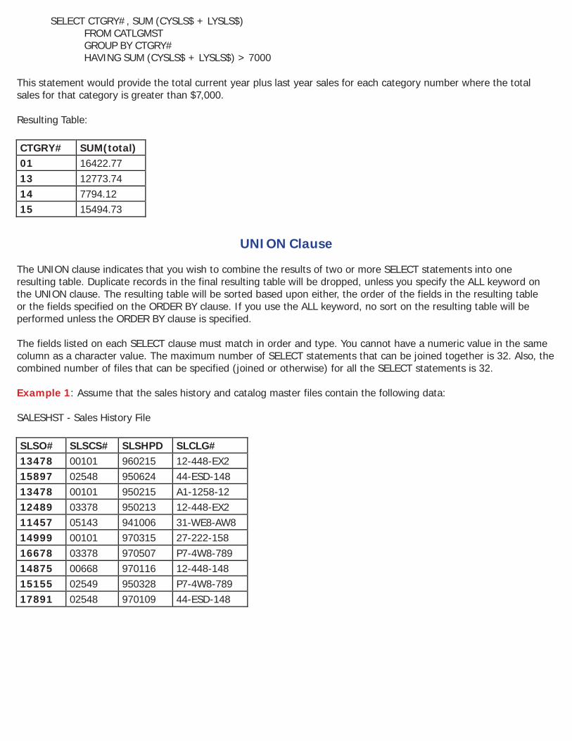
CATLG# CTGRY# CYSLS$ LYSLS$ 12-448-EX2 13 4879.52 7894.22 44-ESD-148 15 278.78 1489.77 A1-1258-12 01 1763.48 1589.44 55-78W-12A 10 2248.97 789.88 31-WE8-AW8 15 879.66 444.48 27-222-158 15 148.79 0.00 P7-4W8-789 14 3915.01 3879.11 2W-877-WW2 22 550.00 2489.45 2W-877-XX1 15 4987.88 7265.37 36Q-456-EQ 01 8793.45 4276.40

SELECT CTGRY#, SUM (CYSLS$ + LYSLS$) FROM CATLGMST GROUP BY CTGRY# HAVING SUM (CYSLS$ + LYSLS$) > 7000

This statement would provide the total current year plus last year sales for each category number where the total sales for that category is greater than $7,000. Resulting Table:

CTGRY# SUM(total) 01 16422.77 13 12773.74 14 7794.12 15 15494.73

UNION Clause The UNION clause indicates that you wish to combine the results of two or more SELECT statements into one resulting table. Duplicate records in the final resulting table will be dropped, unless you specify the ALL keyword on the UNION clause. The resulting table will be sorted based upon either, the order of the fields in the resulting table or the fields specified on the ORDER BY clause. If you use the ALL keyword, no sort on the resulting table will be performed unless the ORDER BY clause is specified. The fields listed on each SELECT clause must match in order and type. You cannot have a numeric value in the same column as a character value. The maximum number of SELECT statements that can be joined together is 32. Also, the combined number of files that can be specified (joined or otherwise) for all the SELECT statements is 32. Example 1: Assume that the sales history and catalog master files contain the following data: SALESHST - Sales History File

SLSO# SLSCS# SLSHPD SLCLG# 13478 00101 960215 12-448-EX2 15897 02548 950624 44-ESD-148 13478 00101 950215 A1-1258-12 12489 03378 950213 12-448-EX2 11457 05143 941006 31-WE8-AW8 14999 00101 970315 27-222-158 16678 03378 970507 P7-4W8-789 14875 00668 970116 12-448-148 15155 02549 950328 P7-4W8-789 17891 02548 970109 44-ESD-148

CATLGMST - Catalog Master File


SELECT DISTINCT SLCLG# FROM SALESHST WHERE SLSHPD >= 970101

UNION SELECT CATLG#

FROM CATLGMST WHERE SUBSTR (DIGITS (CATDTE), 5, 2) >= ‘97’

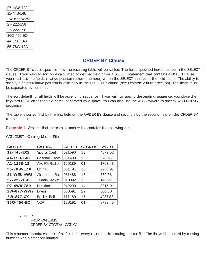
This statement would produce a list of all catalog numbers that have been sold on or since January 1, 1997, or were introduced into the catalog master file after 1997. Records Selected: From SALESHST From CATLGMST

SLCLG# CATLG# P7-4W8-789 2W-877-WW2 12-448-148 27-222-158 27-222-158 36Q-456-EQ 44-ESD-148 55-78W-12A

Final Resulting Table:

P7-4W8-790 12-448-148 2W-877-WW2 27-222-158 36Q-456-EQ 44-ESD-148 55-78W-12A

If you used the UNION ALL instead of just the UNION, you would get the following resulting table.

P7-4W8-790 12-448-148 2W-877-WW2 27-222-158 27-222-158 36Q-456-EQ 44-ESD-148 55-78W-12A

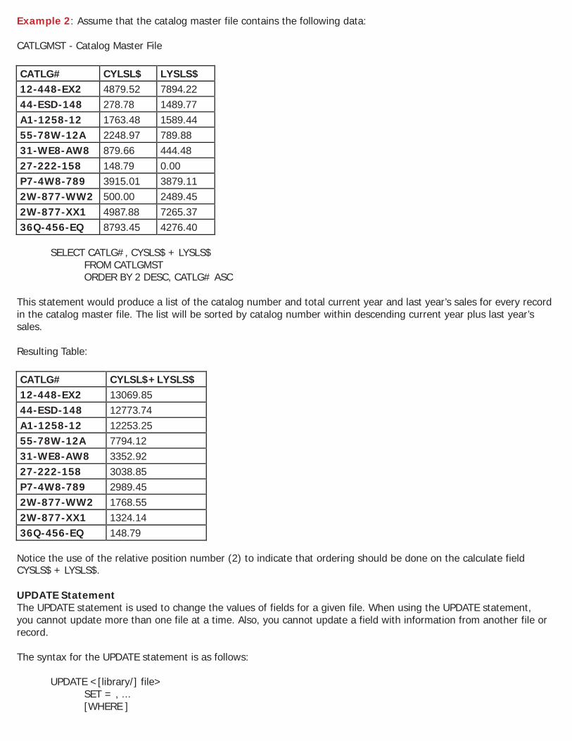
ORDER BY Clause The ORDER BY clause specifies how the resulting table will be sorted. The fields specified here must be in the SELECT clause. If you wish to sort on a calculated or derived field or on a SELECT statement that contains a UNION clause, you must use the field’s relative position (column number) within the SELECT, instead of the field name. The ability to specify a field’s relative position is valid only in the ORDER BY clause (see Example 2 in this section). The fields must be separated by commas. The sort default for all fields will be ascending sequence. If you wish to specify descending sequence, you place the keyword DESC after the field name, separated by a space. You can also use the ASC keyword to specify ASCENDING sequence. The table is sorted first by the first field on the ORDER BY clause and secondly by the second field on the ORDER BY clause, and so. Example 1: Assume that the catalog master file contains the following data: CATLGMST - Catalog Master File


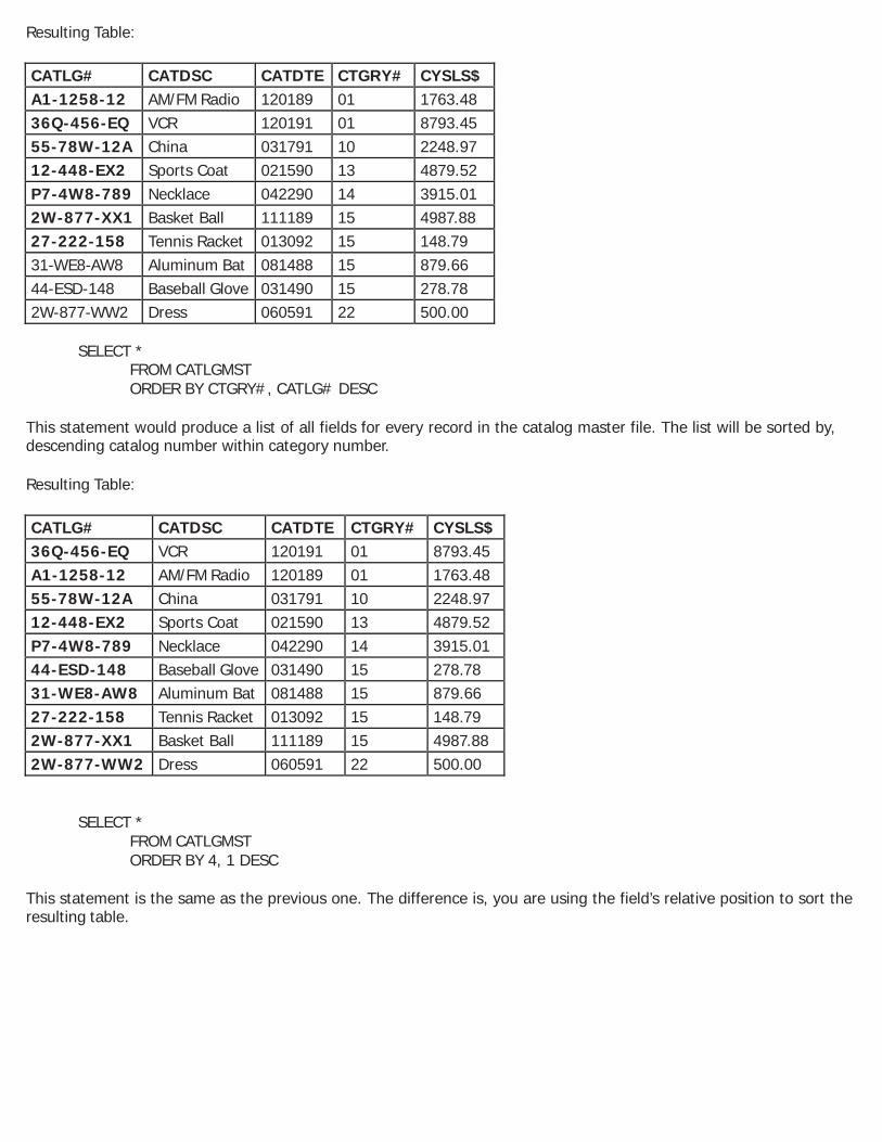
SELECT * FROM CATLGMST ORDER BY CTGRY#, CATLG#

This statement produces a list of all fields for every record in the catalog master file. The list will be sorted by catalog number within category number.

Resulting Table:

CATLG# CATDSC CATDTE CTGRY# CYSLS$ A1-1258-12 AM/FM Radio 120189 01 1763.48 36Q-456-EQ VCR 120191 01 8793.45 55-78W-12A China 031791 10 2248.97 12-448-EX2 Sports Coat 021590 13 4879.52 P7-4W8-789 Necklace 042290 14 3915.01 2W-877-XX1 Basket Ball 111189 15 4987.88 27-222-158 Tennis Racket 013092 15 148.79 31-WE8-AW8 Aluminum Bat 081488 15 879.66 44-ESD-148 Baseball Glove 031490 15 278.78 2W-877-WW2 Dress 060591 22 500.00

SELECT * FROM CATLGMST ORDER BY CTGRY#, CATLG# DESC

This statement would produce a list of all fields for every record in the catalog master file. The list will be sorted by, descending catalog number within category number. Resulting Table:

CATLG# CATDSC CATDTE CTGRY# CYSLS$ 36Q-456-EQ VCR 120191 01 8793.45 A1-1258-12 AM/FM Radio 120189 01 1763.48 55-78W-12A China 031791 10 2248.97 12-448-EX2 Sports Coat 021590 13 4879.52 P7-4W8-789 Necklace 042290 14 3915.01 44-ESD-148 Baseball Glove 031490 15 278.78 31-WE8-AW8 Aluminum Bat 081488 15 879.66 27-222-158 Tennis Racket 013092 15 148.79 2W-877-XX1 Basket Ball 111189 15 4987.88 2W-877-WW2 Dress 060591 22 500.00

SELECT * FROM CATLGMST ORDER BY 4, 1 DESC

This statement is the same as the previous one. The difference is, you are using the field’s relative position to sort the resulting table.

Example 2: Assume that the catalog master file contains the following data: CATLGMST - Catalog Master File

CATLG# CYLSL$ LYSLS$ 12-448-EX2 4879.52 7894.22 44-ESD-148 278.78 1489.77 A1-1258-12 1763.48 1589.44 55-78W-12A 2248.97 789.88 31-WE8-AW8 879.66 444.48 27-222-158 148.79 0.00 P7-4W8-789 3915.01 3879.11 2W-877-WW2 500.00 2489.45 2W-877-XX1 4987.88 7265.37 36Q-456-EQ 8793.45 4276.40

SELECT CATLG#, CYSLS$ + LYSLS$ FROM CATLGMST ORDER BY 2 DESC, CATLG# ASC

This statement would produce a list of the catalog number and total current year and last year’s sales for every record in the catalog master file. The list will be sorted by catalog number within descending current year plus last year’s sales. Resulting Table:

CATLG# CYLSL$+LYSLS$ 12-448-EX2 13069.85 44-ESD-148 12773.74 A1-1258-12 12253.25 55-78W-12A 7794.12 31-WE8-AW8 3352.92 27-222-158 3038.85 P7-4W8-789 2989.45 2W-877-WW2 1768.55 2W-877-XX1 1324.14 36Q-456-EQ 148.79

Notice the use of the relative position number (2) to indicate that ordering should be done on the calculate field CYSLS$ + LYSLS$. UPDATE Statement The UPDATE statement is used to change the values of fields for a given file. When using the UPDATE statement, you cannot update more than one file at a time. Also, you cannot update a field with information from another file or record. The syntax for the UPDATE statement is as follows:

UPDATE <[library/] file> SET = , ... [WHERE ]

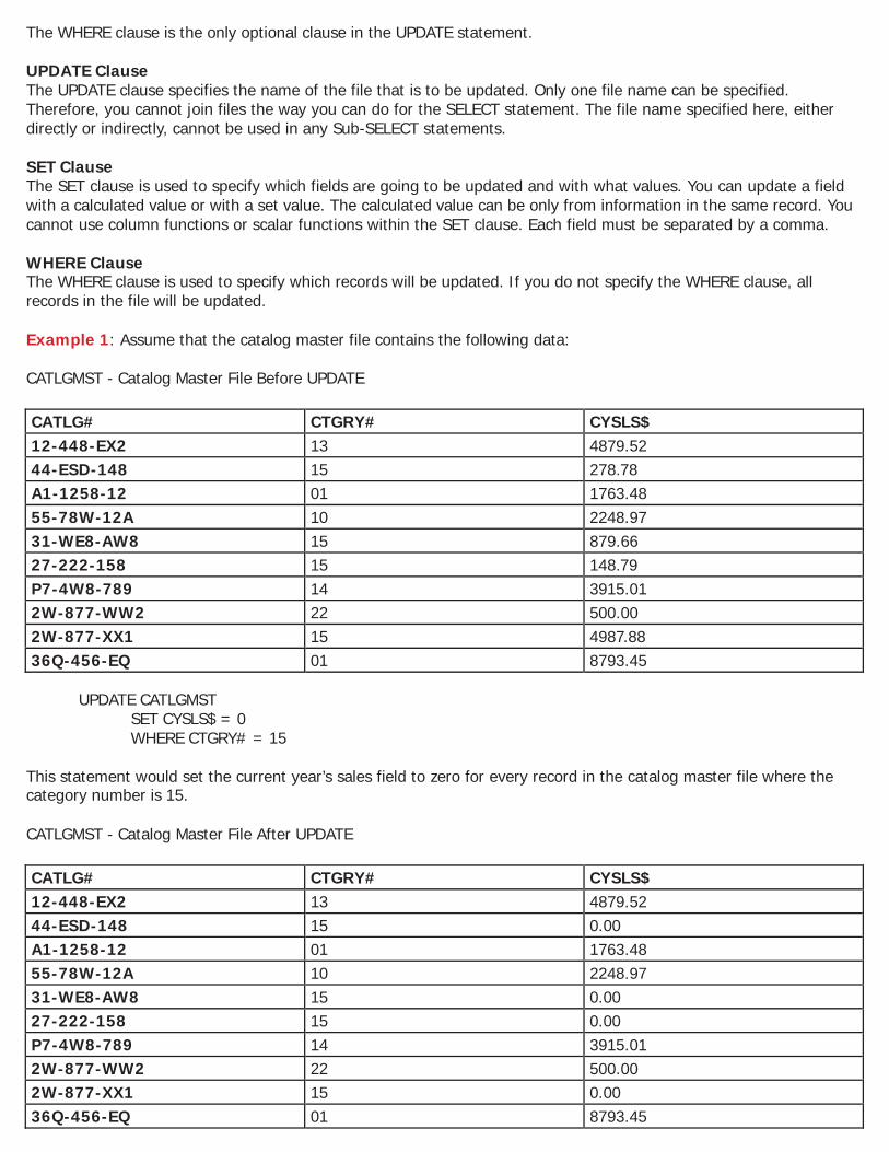
The WHERE clause is the only optional clause in the UPDATE statement. UPDATE Clause The UPDATE clause specifies the name of the file that is to be updated. Only one file name can be specified. Therefore, you cannot join files the way you can do for the SELECT statement. The file name specified here, either directly or indirectly, cannot be used in any Sub-SELECT statements. SET Clause The SET clause is used to specify which fields are going to be updated and with what values. You can update a field with a calculated value or with a set value. The calculated value can be only from information in the same record. You cannot use column functions or scalar functions within the SET clause. Each field must be separated by a comma. WHERE Clause The WHERE clause is used to specify which records will be updated. If you do not specify the WHERE clause, all records in the file will be updated. Example 1: Assume that the catalog master file contains the following data: CATLGMST - Catalog Master File Before UPDATE

CATLG# CTGRY# CYSLS$ 12-448-EX2 13 4879.52 44-ESD-148 15 278.78 A1-1258-12 01 1763.48 55-78W-12A 10 2248.97 31-WE8-AW8 15 879.66 27-222-158 15 148.79 P7-4W8-789 14 3915.01 2W-877-WW2 22 500.00 2W-877-XX1 15 4987.88 36Q-456-EQ 01 8793.45

UPDATE CATLGMST SET CYSLS$ = 0 WHERE CTGRY# = 15

This statement would set the current year’s sales field to zero for every record in the catalog master file where the category number is 15. CATLGMST - Catalog Master File After UPDATE

CATLG# CTGRY# CYSLS$ 12-448-EX2 13 4879.52 44-ESD-148 15 0.00 A1-1258-12 01 1763.48 55-78W-12A 10 2248.97 31-WE8-AW8 15 0.00 27-222-158 15 0.00 P7-4W8-789 14 3915.01 2W-877-WW2 22 500.00 2W-877-XX1 15 0.00 36Q-456-EQ 01 8793.45

Example 2: Assume that the catalog master file contains the following data: CATLGMST - Catalog Master File Before UPDATE

CATLG# CYSLS$ LYSLS$ L2SLS$ 12-448-EX2 4879.52 7894.22 6106.12 44-ESD-148 278.78 1489.77 826.73 A1-1258-12 1763.48 1589.44 2431.64 55-78W-12A 2248.97 789.88 0.00 31-WE8-AW8 879.66 444.48 799.78 27-222-158 148.79 0.00 0.00 P7-4W8-789 3915.01 3879.11 3125.68 2W-877-WW2 500.00 2489.45 0.00 2W-877-XX1 4987.88 7265.37 6241.39 36Q-456-EQ 8793.45 4276.40 0.00

UPDATE CATLGMST SET L2SLS$=LYSLS$ LYSLS$=CYSLS$, CYSLS$=0

This statement would update the two years ago sales field with last year’s sales, then last year’s sales with the current year’s sales and finally set the current year’s sales to zero for every record in the catalog master file. CATLGMST - Catalog Master File After UPDATE

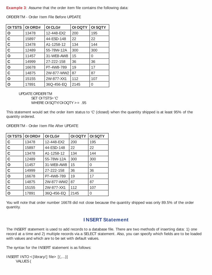
CATLG# CYSLS$ LYSLS$ L2SLS$ 12-448-EX2 0.00 4879.52 7894.22 44-ESD-148 0.00 278.79 1489.77 A1-1258-12 0.00 1763.48 1589.44 55-78W-12A 0.00 2248.97 789.88 31-WE8-AW8 0.00 879.66 444.48 27-222-158 0.00 148.79 0.00 P7-4W8-789 0.00 3915.01 3879.11 2W-877-WW2 0.00 500.00 2489.45 2W-877-XX1 0.00 4987.88 7265.37 36Q-456-EQ 0.00 8793.45 4276.40

Example 3: Assume that the order item file contains the following data: ORDERITM - Order Item File Before UPDATE

OITSTS OIORD# OICLG# OIOQTY OISQTY O 13478 12-448-EX2 200 195 C 15897 44-ESD-148 22 22 C 13478 A1-1258-12 134 144 C 12489 55-78W-12A 300 300 O 11457 31-WE8-AW8 15 0 C 14999 27-222-158 36 36 O 16678 P7-4W8-789 19 17 C 14875 2W-877-WW2 87 87 O 15155 2W-877-XX1 112 107 O 17891 36Q-456-EQ 2145 0

UPDATE ORDERITM SET OITSTS=’C’ WHERE OISQTY/OIOQTY >= .95

This statement would set the order item status to ‘C’ (closed) when the quantity shipped is at least 95% of the quantity ordered. ORDERITM - Order Item File After UPDATE

OITSTS OIORD# OICLG# OIOQTY OISQTY C 13478 12-448-EX2 200 195 C 15897 44-ESD-148 22 22 C 13478 A1-1258-12 134 144 C 12489 55-78W-12A 300 300 O 11457 31-WE8-AW8 15 0 C 14999 27-222-158 36 36 O 16678 P7-4W8-789 19 17 C 14875 2W-877-WW2 87 87 C 15155 2W-877-XX1 112 107 O 17891 36Q-456-EQ 2145 0

You will note that order number 16678 did not close because the quantity shipped was only 89.5% of the order quantity.

INSERT Statement The INSERT statement is used to add records to a database file. There are two methods of inserting data: 1) one record at a time and 2) multiple records via a SELECT statement. Also, you can specify which fields are to be loaded with values and which are to be set with default values. The syntax for the INSERT statement is as follows: INSERT INTO <[library/] file> [(,...)]

VALUES (

UNIT 4

Operators and Functions

SQL Operators In chapter three we briefly covered the operators possible with SQL, now we will go more in depth as to the use of those operators. The SQL operators are grouped into three categories, comparison, logical, and arithmetic (numeric and character). Each category is discussed separately in the following sections.

Comparison Operators Comparison operators return either a true or false value and are most commonly used in the WHERE clause of the SELECT statement to condition which records are chosen from the file or files. Comparison operators are also used in the WHERE clause to form the join specification when two or more files are joined. All of the comparison operators take two operands, which can be of any type, but both operands must be the same type. The SQL comparison operators are:

= Equal to

Not equal

< > Not equal

Greater than

Not Greater than

< Less than

Not less than

>= Greater than or equal to

<= Less than or equal to

Logical Operators Like the comparison operators, the logical operators also return a true or false condition and are most commonly used in the WHERE clause of the SELECT statement. Operands to these operators must be of type logical (true or false value). The logical operators are:

AND syntax: <logical_expr> AND <logical_expr> return: true only if both operands are true, false otherwise.

OR syntax: <logical_expr> OR <logical_expr>

return: false only if both operands are false, true otherwise.

NOT syntax: NOT <logical_expr> return: true if the operand is false, false if the operand is true.

Arithmetic Operators There are two types of arithmetic operators, numeric and character. The numeric operators have an associated precedence or priority of execution. If you do not use parenthesis to group an expression involving numeric operators

this precedence is used to prioritize the order of calculation. The following are the numeric arithmetic operators (their precedence is given in parenthesis with 1 being the highest):

(1) + -

positive sign for a numeric expression negative sign for a numeric expression

(2) ** exponentiation

(3) * /

multiplication division

(4) + -

addition subtraction

There is only one character operator, concatenation. Concatenation adds one character value to the end of another. Programmers familiars with CL will immediately recognize this as the equivalent to the *CAT CL operator. In SQL however, the operator is:

|| OR CONCAT concatenation

SQL Functions SQL also provides some built-in functions that you can use to change how data is presented. The SQL functions are grouped into two categories, scalar and column. Scalar functions operate on a single value and return a value for every record in a SQL statement. Column function operates on a column or group of values returning only a single value for a group of records. In the example,

SELECT ABSVAL (SALES) FROM SALES_FILE the scalar function ABSVAL (absolute value) will return a value for every record in file SALES_FILE, the absolute value of SALES. In the example,

SELECT AVG (SALES) FROM SALES_FILE the column function AVG (compute statistical average) will return only a single value for all the records in SALES_FILE, namely the average of the values in field SALES.

NOTE: Next to each function in the following sections, the earliest release of OS/400, which supports the function, is given in parenthesis. If you attempt to use a function and you are on an earlier release, it will fail.

Scalar Functions Scalar functions are those built-in functions that allow you to change the size and characteristics of a single field. Some scalar functions can be performed on numeric values, some on character values. Scalar functions can be embedded within each other as long as the data type rules are followed. Column functions can be embedded within scalar functions. The following are the scalar functions available: ABSVAL (V2R2) The ABSVAL function returns the absolute value of a number. This function is only valid with numeric fields. The syntax for the ABSVAL function is: ABSVAL (value)

Example:

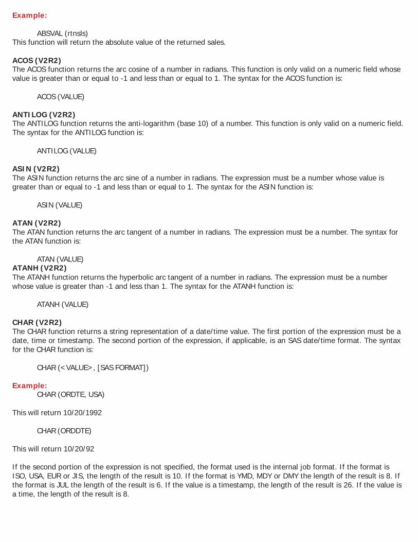
ABSVAL (rtnsls) This function will return the absolute value of the returned sales. ACOS (V2R2) The ACOS function returns the arc cosine of a number in radians. This function is only valid on a numeric field whose value is greater than or equal to -1 and less than or equal to 1. The syntax for the ACOS function is:

ACOS (VALUE) ANTILOG (V2R2) The ANTILOG function returns the anti-logarithm (base 10) of a number. This function is only valid on a numeric field. The syntax for the ANTILOG function is:

ANTILOG (VALUE) ASIN (V2R2) The ASIN function returns the arc sine of a number in radians. The expression must be a number whose value is greater than or equal to -1 and less than or equal to 1. The syntax for the ASIN function is:

ASIN (VALUE) ATAN (V2R2) The ATAN function returns the arc tangent of a number in radians. The expression must be a number. The syntax for the ATAN function is:

ATAN (VALUE) ATANH (V2R2) The ATANH function returns the hyperbolic arc tangent of a number in radians. The expression must be a number whose value is greater than -1 and less than 1. The syntax for the ATANH function is:

ATANH (VALUE) CHAR (V2R2) The CHAR function returns a string representation of a date/time value. The first portion of the expression must be a date, time or timestamp. The second portion of the expression, if applicable, is an SAS date/time format. The syntax for the CHAR function is:

CHAR (<VALUE>, [SAS FORMAT]) Example:

CHAR (ORDTE, USA) This will return 10/20/1992

CHAR (ORDDTE)

This will return 10/20/92 If the second portion of the expression is not specified, the format used is the internal job format. If the format is ISO, USA, EUR or JIS, the length of the result is 10. If the format is YMD, MDY or DMY the length of the result is 8. If the format is JUL the length of the result is 6. If the value is a timestamp, the length of the result is 26. If the value is a time, the length of the result is 8.

COS (V2R2) The COS function returns the cosine of a number. This function is only valid for numeric fields. The syntax for the COS function is:

COS (VALUE) COSH (V2R2) The COSH function returns the hyperbolic cosine of a number. The expression must be a number whose value are specified in radians. The syntax for the COSH function is:

COSH (VALUE) COT (V2R2) The COT function returns the cotangent of a number. The expression must be a number whose value is specified in radians. The syntax for the COT function is:

COT (VALUE) DATE (V2R1M1) The DATE function returns a date from a value. The field must be a date, timestamp, valid string representation of a date, character string with a length of 7 or a positive number less than or equal to 3652059. The syntax for the DATE function is:

DATE (VALUE) If the field is a timestamp then the result would be the date portion of the timestamp. If the field is a number then the result would be the number of days after January 1, 0001. If the field is a character string then the result would be the internal default CCSID converted to a date. DAY (V2R1M1) The DAY function returns the day portion of a value. The field must be a date, timestamp, date duration or timestamp duration. The syntax for the DAY function is: DAY (VALUE) If the field is a date or timestamp then the result would be the day portion of the value which is a number between 1 and 31. If the field is date duration or a timestamp duration then the result would be the day portion of the value, which is a number between -99 and 99. DAYS (V2R1M1) The DAYS function returns a numeric representation of a date. The value must be a date, timestamp or a valid string representation of a date. The result is 1 more than the number of days from January 1, 0001 to the date that would occur if you applied the DATE function to the value. The syntax for the DAYS function is:

DAYS(VALUE) DECIMAL (V1R3) The DECIMAL function allows us to define the size of a numeric field. This is useful, when we wish to present a calculated value with a specific size, instead of the default size. You must be careful that significant digits are not truncated when sizing the value. If this happens, the statement being executed will fail. This syntax for the DECIMAL function is:

DECIMAL (value, size, decimals) Example:

DECIMAL (ORDQTY*PRICE, 9, 2)

This function will multiply the order quantity by the price and place the result in a field with a size of 9.2. DIGITS (V1R3) The DIGITS function allows us to convert a number to a character value. The syntax for the DIGITS function is:

DIGITS(value) Example:

DIGITS(ORDDTE) This function will convert the numeric order entry date to a character value. You will notice that there are no functions to convert a string value into a numeric value. This will severely restrict your ability to manipulate a file with no external definition. EXP (V2R2) The EXP function returns a value that is the base of the natural logarithm raised to the power specified by the value. This function is only valid with numeric values. The syntax for the EXP function is:

EXP(VALUE) FLOAT (V1R3) The FLOAT function allows us to convert a number into a floating point number. The syntax for the FLOAT function is:

FLOAT (value) Example:

FLOAT(ORDQTY*PRICE) This function will multiply the order quantity by the price and present the result as a floating point number. HEX (V2R1M1) The HEX function returns a hexadecimal representation of a value. The value can be a character or numeric data type. The result of the function is a character string that is twice the length attribute of the value. The syntax for the HEX function is:

HEX (VALUE) HOUR (V2R1M1) The HOUR function returns the hour portion of a value. The value must be a time, timestamp, time duration or a timestamp duration. If the value is a time or timestamp then the result will be a number between 0 and 24. If the value is a time duration or timestamp duration then the result will be a number between - 99 and 99. The syntax for the HOUR function is:

HOUR(VALUE) INTEGER (V1R3) The INTEGER function allows us to convert a number into an integer value. The syntax for the INTEGER function is:

INTEGER(value)

Example:

INTEGER(PRICE)

This function will convert the price field into an integer value.

LAND (V2R2) The LAND function returns a string that is the logical AND of the argument strings. This function takes the first argument string, does an AND comparison with the next string, and then continues to do AND comparisons with each successive argument using the previous result. If an argument is shorter than the previous result then it is padded with blanks. This function is only valid with character strings, however they cannot be mixed character strings. There must always be two or more arguments. The resulting length is the same as that of the longest argument. The syntax for the LAND function is:

LAND(VALUE1, VALUE2 [, . . .])

LENGTH (V1R3) The LENGTH function returns the length of a value. The length returned represents the number of positions that are required to store the value, excluding trailing blanks. The value checked can be either numeric or character. The syntax for the LENGTH function is:

LENGTH(value) Example:

LENGTH(CATDSC) This function will return the length of the catalog description field. LN (V2R2) The LN function returns the natural logarithm of a number. The value must be a number. The syntax for the LN function is:

LN(VALUE) LOG (V2R2) The LOG function returns the common logarithm of a number. This function is only valid with numeric values. The syntax for the LOG function is:

LOG(VALUE) LOR (V2R2) The LOR function returns a string that is the logical OR of the argument strings. This function takes the first argument string, does an OR comparison with the next string, and then continues to do OR comparisons for each successive argument using the previous result. If an argument is shorter than the previous result then it is padded with blanks. The arguments must be character strings, however they cannot be mixed character strings. There must be two or more arguments. The resulting length is the same as that of the longest argument. The syntax for the LOR function is:

LOR (VALUE1, VALUE2 [, . . .]) LNOT (V2R2) The LNOT function returns a string that is the logical NOT of the argument string. The argument must be a character string, however it cannot be a mixed character string. The syntax for the LNOT function is:

LNOT(VALUE) MAX (V2R2) The MAX scalar function returns the maximum value in a set of values. This function is only valid with two or more arguments whose data types are compatible. The maximum length allowed for a character string is 255. The result of the function is the largest argument value. The syntax for the MAX scalar function is:

MAX (VALUE1, VALUE2 [, . . .])

MICROSECOND (V2R1M1) The MICROSECOND function returns the microsecond portion of a value. The value must be a timestamp, a string representation of a timestamp or a timestamp duration. The syntax for the MICROSECOND function is:

MICROSECOND(VALUE) MIN (V2R2) The MIN scalar function returns the minimum value for a set of values. This function is only valid with two or more arguments whose data types are compatible. The maximum length allowed for a character string is 255. The result of the function is the largest argument value. The syntax for the MIN scalar function is:

MIN(VALUE1, VALUE2 [, . . .]) MINUTE (V2R1M1) The MINUTE function returns the minute portion of a value. The value must be a time, timestamp, time duration or timestamp duration. The syntax for the MINUTE function is:

MINUTE(VALUE) MOD (V2R2) The MOD function divides the first value by the second value and returns the remainder. The values must be numbers and the second value cannot be a zero. The syntax for the MOD function is:

MOD(VALUE1, VALUE2) MONTH (V2R1M1) The MONTH function returns the month portion of a value. The value must be a date, timestamp, date duration or timestamp duration. If the value is a date or a timestamp, then the result is a number between 1 and 12. If the value is a timestamp duration or a date duration, then the result is a number between -99 and 99. The syntax for the MONTH function is:

MONTH(VALUE) SECOND (V2R1M1) The SECOND function returns the seconds portion of a value. The value must be a time, timestamp, time duration or timestamp duration. If the value is a time or timestamp, then the result is a number between 1 and 59. If the value is a time duration or timestamp duration, then the result is a number between -99 and 99. The syntax for the SECOND function is:

SECOND(VALUE)

SIN (V2R2) The SIN function returns the sine of a number. The value must be a number specified in radians. The syntax for the SIN function is:

SIN(VALUE) SINH (V2R2) The SINH function returns the hyperbolic sine of a number. The value must be a number specified in radians. The syntax for the SINH function is:

SINH(VALUE) SQRT (V2R2) The SQRT function returns the square root of a number. The value must be a positive number. The syntax for the SQRT function is:

SQRT(VALUE)

STRIP (V2R1M1) The STRIP function removes blanks or another specified character from the beginning or end of a string expression. The first value must be a string expression. The second value indicates whether characters are removed from the beginning or end of the string. The possible syntax for the second value are: B for both, L for leading and T for trailing. If no second value is specified then blanks are removed from both the beginning and end of the string. The third value specifies which single character constant is to be removed. If no third value is specified then the default strip character is a blank. The syntax for the STRIP function is:

STRIP ([, STRIP POSITION] [, STRIP CHARACTER]) SUBSTR (V1R3) The SUBSTR function allows us to extract a portion of a string value. The syntax for the SUBSTR function is:

SUBSTR (string,start,length) You must be careful that the starting position and length specified do not exceed the actual length of the string. If this happens, the statement will fail. This is the function that you use if you wish to extract data from a file with no external definition. Example:

SUBSTR (CATLG#,1,10) This function will extract the first 10 characters of the catalog number. TAN (V2R2) The TAN function returns the tangent of a number. The value must be a number specified in radians. The syntax for the TAN function is:

TAN(VALUE) TANH (V2R2) The TANH function returns the hyperbolic tangent of a number. The value must be a number specified in radians. The syntax for the TANH function is:

TANH(VALUE) TIME (V2R1M1) The TIME function returns a time from a value. The value must be a time, timestamp or a valid string representation of a time. The syntax for the TIME function is:

TIME(VALUE) TIMESTAMP (V2R1M1) The TIMESTAMP function returns a timestamp from a value or pair of values. If only one argument is specified then it must be a timestamp, valid string representation of a timestamp or a character string with a length of 14. The character string must be digits representing a valid date and time in the form yyymmddhhmnmss. If both arguments are specified then the first argument must be a date or valid string representation of a date, and the second argument must be a time or valid string representation of a time. The syntax for the TIMESTAMP function is:

TIMESTAMP ([, VALUE2])

TRANSLATE (V2R2) The TRANSLATE function translates the characters of the value to uppercase. The value must be a character string or mixed character string, however, it cannot be a graphic string. The syntax for the TRANSLATE function is:

TRANSLATE(VALUE)

VALUE (V2R1M1) The VALUE function returns the first argument that is not null. There must be two or more arguments and they must have compatible data types. The arguments are evaluated in the order which they are specified. The syntax for the VALUE function is:

VALUE (VALUE1, VALUE2 [, . . .]) XOR (V2R2) The XOR function returns a string that is the logical ‘XOR’ of the argument strings. This function takes the first argument string, does an ‘XOR’ comparison with the next string, and then continues to do ‘XOR’ comparisons for each successive argument using the previous result. If an argument is shorter than the previous result, it is padded with blanks. There must be two or more arguments and they must be character strings, however, they cannot be mixed character strings. The syntax for the XOR function is:

XOR (VALUE1, VALUE2 [, . . .]) YEAR (V2R1M1) The YEAR function returns the year portion of a value. The value must be a date, timestamp, date duration or timestamp duration. If the value is a date or timestamp then the result is a number between 1 and 9999. If the value is a date duration or timestamp duration then the result is a number between -9999 and 9999. The syntax for the YEAR function is:

YEAR(VALUE) ZONED (V2R2) The ZONED function returns a zoned decimal representation of a number. The first argument must be a number. The second argument, if specified, must be a number between 1 and 31. The third argument, if specified, must be a number between 0 and the value of the second argument. If the third argument is not specified then the default is zero. The default for the second argument is either 5 for small integer, 11 for large integer or 15 for floating-point, decimal, numeric or non-zero scale binary. The syntax for the ZONED function is:

ZONED([, PRECISION, SCALE])

Column Functions Column functions perform an operation over a group of records and return a single result for each group (see GROUP BY clause). For example, you can obtain the average amount for a group of invoice records. Column functions can only be used in the SELECT and HAVING clauses. You can obtain a column function figure for an entire file or you can obtain figures for subgroups of records by using the GROUP BY clause.

You cannot embed column functions within each other.

The following are the column functions available:

AVG (V1R3) The AVG function returns the average value for a numeric field in a group of records. The syntax for the AVG function is:

AVG(value)

Examples:

AVG(CYSLS$) This function would return the average of the current year sales for each group selected.

AVG(CYSLS$+LYSLS$) This function would return the average of the total of the current and last year sales for each group selected. COUNT(*) (V1R3) The COUNT function returns the number of records found within a group. The result is a number. There are no values used with the COUNT function. Example:

COUNT (*) MAX (V1R3) The MAX function returns the maximum value encountered for a group of records. This function can be performed on numeric or character fields. When processing a character field, the result cannot exceed 256 characters. The syntax for the MAX function is:

MAX(value) Examples:

MAX (SLSAMT) This function will return the maximum sales amount found for the group selected.

MAX (SUBSTR (DIGITS (ORDTE), 5, 2) This function will return the maximum year found in the order entry date for the group selected. Notice that we used several built-in functions to extract the year. MIN (V1R3) The MIN function returns the minimum value found for a group of records. This function can be performed on numeric and character fields. When processing a character field, the result of the MIN function cannot exceed 256 characters. The syntax for the MIN function is:

MIN(value) Examples:

MIN (SLSAMT) This function will return the minimum sales amount found for the group selected.

MIN (SUBSTR (DIGITS (ORDDDTE), 5, 2) This function will return the minimum year found in the order entry date for the group selected. Notice that we used several built-in functions to extract the year. STDDEV (V2R2) The STDDEV function returns the biased standard deviation for a set of numbers. This function is valid only on numeric fields. The syntax for the STDDEV function is:

STDDEV(value) Examples:

STDDEV (SLSAMT)

This function will return the standard deviation for the total sales amount for each group selected.

SUM (V1R3) The SUM function returns the total value for a group of records. This function is valid only for numeric fields. The syntax for the SUM function is: SUM(value) Example:

SUM(CYSLS$) This function will return the sum of the current year sales for the group selected. VAR (V2R2) The VAR function returns the biased variance for a set of numbers. This function is only valid for numeric fields. The syntax for the VAR function is: VAR(value) Example:

VAR(PRICE) This function will return the variance of price for the group selected.

UNIT 5

Embedded Variables A powerful feature of SQL/PRO is the ability to use variables within your SQL statements. What this means is that you can let the system either prompt you for a value or pass a value through a parameter and its value will be substituted into your SQL statement at execution time. For example, you want your users to be able to create a list of customers for any state they choose. Instead of creating 50 different saved queries (one for each state) you can simply create one query that uses a variable in place of the state value. A variable is defined by starting a string with an ‘&’character. The following SQL statement would be all you would need to create the query for the above example:

SELECT * FROM CUSTMAST WHERE CMSTE = &STATE

A variable can be placed anywhere within an SQL statement (in place of a column name, a file name, an operator or a compare value just to mention a few), but no more than 50 can be used. The user gains the added benefit of being able to run the query in batch. At execution time the system will prompt the user for a value for variable STATE. Since CMSTE is a character data type it is required that the value be submitted within apostrophes. If an SQL statement containing variables is saved, values can be passed to it through the STRQMAQRY command. This way the system doesn’t need to prompt you for the value/s at execution time. To illustrate, here is the STRQMQRY command necessary to run the above statement using AZ as the state:

STRQMQRY QMQRY (LSTCSTMST) OUTPUT (*PRINT) SETVAR ((STATE ‘’’’AZ’’’’))

Since the command processor removes the outer apostrophes and converts embedded double apostrophes to single the SQL statement resolves to look like this:

SELECT * FROM CUSTMAST WHERE CMSTE = ‘AZ’

A CL variable could be used in place of the character constant. The format for the CHGVAR command could look like this:

DCL VAR(&QUOTE) TYPE(*CHAR) LEN(2) VALUE(‘’’’) DCL VAR(&STATE) TYPE(*CHAR) LEN(4)

CHGVAR VAR (&STATE) VALUE (&QUOTE |< ‘AZ’ |< &QUOTE)

NOTE: “|<” is a concatenation symbol

The CHGVAR command (as well as any command that accepts character strings) strips the outermost single apostrophes and converts each inner set of two apostrophes to one. Therefore, the &STATE variable ends up with “AZ” as we desire.

The STRQMQRY command could now be coded as:

STRQMQRY QMQRY (LSTCSTMST) OUTPUT (*PRINT) SETVAR ((STATE &STATE))

This method also allows you to replace the character constant with a CL variable so that different values can be entered at run time from a display file or another program. Passing numeric values is much easier since apostrophes aren’t required. To pass a variable to the following SQL statement:

SELECT * FROM CUSTOMAST WHERE CMPDUE = &PDCTR

This segment of CL code could be used:

CHGVAR VAR (&PASTDUECTR) VALUE (6)

STRQMQRY QMQRY (LSTCSTMST) OUTPUT (*PRINT) SETVAR ((PDCTR &PASTDUECTR))

UNIT 6

Formatting Your Reports Without the Report Designer, SQL/PRO only creates a simple listing using a default report format, which prints the values of the columns of the SELECT statement in the order they occur in the statement. The column names are used as heading constants above each column. This is the extent of the default report format. Now with SQL/PRO’ report Designer you can quickly and easily create sophisticated reports. The SQL/PRO Report Designer allows you to format the results of any SQL SELECT statement. You can also create summary information and perform several arithmetic operations. The Report Designer supports most of the requirements for a standard production report:

» The order of the columns

» The horizontal and vertical position of the information

» Meaningful column and page headings

» Control group summary operations

» Separators to highlight headings and summary data

» Text and summary data for the end of the report

With some advance techniques you can produce reports that are much more sophisticated than you might imagine.

For example:

» Character edits that keep long strings on multiple lines of a report but in the same column

» First and last summary functions

» SQL column data in headers and footers

When a query is saved the report formatting for the query is also saved. The following sample report gives you an idea of what can be done with SQL/PRO report formatting. We will lead you through each step of the format process that would create this report so you can get an overview of how it’s done. The format function is identified by the labels to the right of the report. As we go through each of the functions in detail, refer to this report. To begin designing a report, select F22 (Edit report format) from the main SQL/PRO screen and you will be transferred to the Report Designer main screen where you can specify your report functions and format. Initially SQL/PRO will create a default form for you. A report format record will be created for each column specified in your SELECT statement. If you use the ‘*’ in your SELECT statement, a record will be created for every column in the table. On subsequent requests for report format editing (F22), within the same session, SQL/PRO will present a window informing you that a form already exists. Online help is available from anywhere within the Report Designer. Press the help key or F1 to access the online help. The online help is cursor sensitive, so position your cursor on the phrase in question before accessing help. You can choose to change the existing form or re-create a new default form. Typically you will change an existing form unless you change the file from which you are retrieving your information in which case you would want to recreate a default form. The Edit report format function presents the Report Designer panel.

In this example we are creating a control group for District and summarizing the total order amount for each group.

To add a column use F6. A blank column will be inserted after the column in which the cursor is located. To delete a column use F14. The column in which the cursor is located will be deleted. There must be at least one column in a

report format (the system will not let you delete a column if it is the last one in the report format). F7 displays the Design Report Header window and allows you to enter up to five lines of header text. You can see the prompt at the top of the window requesting for the number of lines to skip before and after the header text prints. If these are left blank the header text will simply print on line one. For every text line entered, a “Justify” option of LEFT, CENTER or, RIGHT must be selected to specify the text alignment on the page. F8 presents the Design Report Footer screen. This screen is exactly the same as the report header except that the text lines entered will print at the bottom of the report. Here, we are placing the name of the saved query. To create control group header text use F10. You will be prompted for break header text for each column with a control break specified in the USASGE column (a maximum of six groups can be created, BREAK1 to BREAK6). Again you are prompted for the number of blank lines to skip before and after the text prints, but you also have two new options: Print on new page and repeat column text. These both default to NO but entering YES in the first option will cause a page break and a YES in the second will reprint the column heading text immediately following the break header. Typically, if YES is specified in Print on new page you would leave the repeat column text at NO since the column text is printed automatically on every new page anyway. Take particular notice of the ‘&1’ in the break text. The ampersand followed by a number tells the report format to print the value of the nth data column from the SQL SELECT statement. In this case the first data column contains the break field DISTRICT. Any number of data columns may be inserted in this way and is not limited to the break fields. F11, like F10, will prompt you for footer text for each break field. Again, the example has an embedded variable, ‘&1’, to pull in the DISTRICT. The justification LEFT tells the report format to print the break footer text to the immediate left of the first summary column. RIGHT, then, will print to the right of the last summary column. The report final text (F9), again, works essentially the same as the other report sections except that the final text allows for ten lines of text instead of the header and footer limitation of five. Function key 22 brings up the Modify Standard Report Defaults screen. You will rarely use this screen if you are happy with the defaults specified. Review the previous report example to see what the standard defaults look like. Now that you know how to create report headers and footers, let’s go over the formatting of the detail data. The main screen has a record for each column in the SQL SELECT statement. Most of the editing can be done from the main report designer screen except that the column header text entry field allows for only 27 characters to be entered. Whenever a column heading exceeds 27 characters or is to list on multiple lines of text, use the Extended Column Edit screen accessible with a 2 option. The extended column edit allows you to enter up to four lines of column heading per data column. There is, however, a limitation of a total of 62 characters per column heading. The Usage edit is the real power option to the report designer. Here is where you specify the break fields (which should correspond tot he ORDER BY fields on the SQL SELECT statement) and the summary functions. The usage options are:

OMIT, AVG, COUNT, FIRST, LAST, MAX, MIN, SUM, BREAK1 - BREAK6 Most of these are obvious and there is help text available if you position the cursor in the usage field and press F1 or HELP. I will however mention two of the more obscure options: OMIT and COUNT. Omit simply specifies that a column is not to appear on the report. COUNT lists the total number of detail lines that were a part of the summary data group break. Notice also that only one usage can be specified per column. The edit code is where you definitely will use the F1 Help function. These SQL edit codes are not the same ones that AS/400 programmers are familiar with from SDA, RPG, and Query/400, but the help text is very straightforward. The edit codes include numeric, date, time and several interesting character edits. The field length and decimal position represents the width to display on the report - it does not have to correspond to the actual physical data length in the file. If a numeric value exceeds the width specified, the report will display all

asterisks in that data column. The column indent is the number of spaces from one data column to the previous data column. The column sequence allows you to override the placement of a data column on a report. You may have keyed a long SQL SELECT statement and no longer want the report column sequence to default to the column placement from the SQL. With the sequence number you can easily move columns on a report without changing the SQL statement. The data type is set on the automatic build of the form but on column adds (F6) you need to specify the appropriate type. Don’t worry about whether not the field is packed or zoned - the report designer sees all numbers as NUMERIC. Version 2 enthusiasts will also be happy to know that DATE and TIME data types are available with SQL/PRO’ Report Designer. The extended column edit screen will automatically be displayed when you select the add function (F6). Remember: The number and data type of report format columns must always agree with that of the SQL SELECT statement. This is where the Display SQL Function (F3) comes in handy. Again, if you add or delete a column from the SQL statement you must also add (F6) or delete (F14) from the report form.

Advanced Report Formatting Techniques

Multi-level reports Many databases have files with one-to-many relationships. An example of a one-to-many relationship is a sales order header and sales order detail. Formatting a report that joins two such files is a problem since the header information is duplicated for every detail record. Forget trying to create a clean report of this nature with Query/400, but with SQL/PRO’s Report Designer and a few simple techniques it can be fairly easy. Using a Sales Order Picklist as an example the following steps describe how to create a multi-level report. On the SQL SELECT:

» Duplicate the break fields.

» Concatenate a blank to the beginning of each break field. If the break is numeric use the SQL digits()

function to convert it to character.

SELECT ORDNBR, ‘ ‘ ||ORDNBR, ORDDTE, LINITM, LINQTY, LINPRC, LINQTY * LINPRC FROM ORDHDR, ORDDTL WHERE ORDHDR.ORDNBR = ORDDTL.ORDNBR ORDER BY ORDNBR

On the Report Design:

» Specify the concatenated ORDER BY duplicate as the break field and set the column width of the break field

to 1 so that only the blank portion of the break will list on the report (you can’t omit a break column)

» Set USAGE to OMIT for all other header fields

» Design a Break header with the header columns specified to print in the header.

Date Edits Dates are a bit of a problem with Report Designer. We do not have the old six digit numeric date edit of Y available to produce a formatted date. But there are two other methods of editing a date: Method One The first way to edit a date is to substring it into its individual month, day, and year fields in the SQL SELECT

statement and concatenate. For instance, to edit a year-month-day date to MM/DD/YY use:

substr (datefld, 3,2) | |’/’| |substr (datefld, 5, 2) | |’/| |substr (datefld, 1,2) Method Two Another way is to use the date edits provided with the Report designer. These edits, through, only work with the new OS/400 Version 2 date types. But you don’t have to wait for date and time fields to be in your database. What you do is convert your old format date into a Version 2 date field by combining Method One to create a date that matches your system date format and then enclose the manually edited date with the SQL DATE () function. Then select any of myriad of date edits available in the Report Designer (see the F1 field text on the main screen). Why go to all this trouble since it uses Method One anyway? By converting your database dates into Version 2 date data type you can then use date math capabilities. This makes calculating such things as the number of days between dates and the maturation of notes a breeze.

Address Formatting A neat trick that the Report Designer will do for you is to format an address. How often have you done lists where a full address was required? But two or three address lines; a name; and the city, state, and zip code takes up too many columns on the report. This leaves too few columns available on the report to print anything else. How would you like to print something like this?:

This technique requires the following steps:

On the SQL SELECT

» Find the longest address line. For example: address line one may be 40 characters but the City, State, and Zip

might exceed 50 with the embedded blanks.

» In the SQL concatenate all fields together adding blank strings so each address line is the length of the longest

line.

For instance, if the name, address line 1, and address line 2 are 40 bytes and the city/state/zip combination is 50 including the concatenated comma and blanks:

Select name ||’ ‘|| ad1||’ ‘|| ad2||’ ‘|| strip (city) ||’,’||state||’ ‘||zip, purch, amtpaid, amtdue

(Notice the column function we use with the city: strip(city). This strips the trailing blanks from the city.)

On the Report Format

» Change the column heading for the concatenated column to something meaningful since by default it will

contain concatenation characters. Here, we change it to Customer address.

» Set the field width to longest field address line (50 in the example).

» Specify the CT character edit code to concatenated address.

» The CT character edit will then wrap the columns to the next line of the report when the column width has

been exceeded (50 in the example).

Standard Headers The Report Designer defaults to automatically printing the current date, time, and page number on the bottom of the report. This works quite well but many users are so used to having the date, time and page at the top of the report

that they now expect it. To do this with the Report Designer is easy; simply enter &DATE, &TIME and &PAGE (all caps) in the report header. The problem with the report formatter though, is that the justify option prints to the left, right, or the center of the report. Users want the date, time, and page at opposite ends of the report. So - fake it. Put the &DATE and &TIME on the first line of the report header left justified. Then put the &PAGE on the second line of the report right justified. Finally, put your report title on line three and center it. Remember, through, if you use &DATE, &TIME and &PAGE on a report for a saved query and later run the query with the STRQMQRY command, you could end up with date, time and/or page on the report twice (wherever you place it and at the bottom of each page). This is because the STRQMQRY command will place the date, time, and page number at the bottom of every page of any query report if the DATETIME and PAGE parameter values are set to *YES (the default).

Dynamic Reports One of the most powerful features of SQL/PRO is its support of variables allowing us to create dynamic reports. All that is required is to create an SQL SELECT statement that has variable selection criterion in the WHERE clause.

SELECT CUSNBR, NAME, ADDRESS FROM CUSMAS WHERE &WHERE

Any word prefixed by an ampersand is seen as a variable to SQL/PRO. The Variable is then set at run time in the STRQMQRY command by keying the variable name in the VAR parameter (make sure to use the same case as is specified in the SQL but without the ampersand) and the dynamic selection in the VALUE parameter. Note that triple quotes are required for character strings; numeric data should have NO quotes or else the system will see the value as a string.

STRQMQRY QMQRY (YOURQRY) QMFORM (YOURQRY) VAR (WHERE) + VALUE (‘’’AMTDUE > 100.00 ‘’’)

This powerful feature allows you to create reports where the user can dynamically set the selection criterion. But the report header should contain the selection criterion or else the user will not know what it is. The solution to this problem is to list the selection criterion on the report by putting the variable on the report header or footer. To do this you need to add the variable to the column list of the SQL SELECT since the Report Designer only supports variable data from the SELECT list.

SELECT CUSNBR, NAME, ADDRESS, PHONE FROM CUSMAS WHERE & PHONE

Then put that data column in the report header or footer and OMIT in the USAGE column in the detail data. The dynamic selection will then always print on the report. You can make slick use of this technique by coding a command or HLL screen with a wide range of prompts to assist the user through the entry of the selection logic.

UNIT 7

SQL/PRO Security

Accessing SQL/PRO Security Make sure that you are signed on as security officer (QSECOFR) and have added the library PDSQL30 to your library list. Enter STRPDSQL on the command line. Now press F13 for the Services menu.

Figure 7.1 Option 7: Security will appear at the bottom of the list. Take option 7 to work with security settings.

Figure 7.2

When you elect to do an Add or Change the next screen appears. Place a “Y” or “N” in each field to denote the functions that the profile will have access to.

Figure 7.3 *PUBLIC is the default user profile. It is initially set up to have no authorities. This profile is used as the default if a user’s individual or group profile is not found. When a user starts SQL/PRO the security program will first look for the user profile then the group profile of the person signing on. The profile being used will appear in the upper right hand corner of the main SQL/PRO screen.

Appendix A

De-Installing SQL/PRO If you ever decide to de-install SQL/PRO, you should follow these steps:

1. Remove SQLPRO from your library list. 2. Remove SQLPRO from your system.

Note: If you are only temporarily removing SQL/PRO, make sure to make a backup copy first. Then reinstall SQL/PRO from this backup. If you do not, you will lose your Saved Queries and history.

Appendix B

SQL Keywords The following words are considered SQL keywords and therefore cannot be used to name objects.

ALL AND ANY AS ASC AUTHORIZATION AVG BEGIN BETWEEN BY CHAR CHARACTER CHECK CLOSE COBOL COMMENT COMMIT CONNECT CONTINUE COUNT CREATE CURRENT CURSOR DATE DEC DECIMAL DECLARE DEFAULT DELETE DESC DISTINCT DOUBLE DROP END ESCAPE EXEC EXISTS FETCH FLOAT FOR FOREIGN FORTRAN FOUND FROM GO GOTO GRANT GROUP HAVING IN INDICATOR INSERT INT INTEGER INTO IS KEY LANGUAGE LIKE MAX MIN MODULE NOT NULL NUMERIC OF ON OPEN OPTION OR ORDER PASCAL PLI PRECISION PRIMARY PRIVILEGES PROCEDURE PUBLIC REAL REFERENCES REVOKE ROLLBACK SCHEMA SECTION SELECT SET SMALLINT SOME SQL SQLCODE SQLERROR SUM TABLE TIME TIMESTAMP TO UNION UNIQUE UPDATE USER VALUES VIEW WHENEVER WHERE WITH WORK

Date post:	03-Apr-2018
Category:	Documents
Upload:	dinhdiep
View:	234 times
Download:	1 times

SQL / Pro - ProData - Custom AS400 Software - dodbu.com · Either select the iSeries (AS/400) host...

Documents