71
1 Big Data Analysis Project Group #18 Aaron Fuhrman Jessica Demuro Wilson Tapia AJW Consultants, Inc. The Pennsylvania State University 12/9/14
| Date post: | 15-Jul-2015 |
| Category: |
Documents |
| Upload: | aaron-fuhrman |
| View: | 81 times |
| Download: | 0 times |

1
Big Data Analysis Project
Group #18
Aaron Fuhrman
Jessica Demuro
Wilson Tapia
AJW Consultants, Inc.
The Pennsylvania State University
12/9/14

2
Big Data Analysis Project
Aaron Fuhrman
Jessica Demuro
Wilson Tapia
AJW Consultants, Inc.
The Pennsylvania State University
12/9/14
Table of Contents
1.)
Introduction………………………………………………………………………………….2
2.) Methods………………………………………………………………………………….5
2.1) Moving Average and Exponential Smoothing………………………………....3
2.2) Regression Analysis…………….………………………………………………4
2.3) K-Means Clustering…………………………….……………………………...4
2.4) Regression……………………………………………………………………. 7
3) Results……………………………………………………………………………………5
Introduction:
This assignment uses predictive analytics methods to analyze the given transaction data
and make meaningful recommendations for the store manager to improve sales. Predictive analytics calculations including moving average, exponential smoothing, linear regression and
kmeans clustering are used and included in this report. There is a wide variety of data included
in the transaction data that varies from week to week.
The first calculation in this analysis is a moving average and exponentia l smoothing
calculation which calculates the prediction error for weeks 10 through 20 of the given data. The
Mean Squared Error, Mean Absolute Deviation, and Tracking Signal are then calculated from the
given data. The next calculation involves a regression analysis of the given transaction data. Lastly, the kmeans clustering algorithm is used to cluster the customers in the database based on
their buying patterns. The data is then analyzed and used to make a final conclusion about the
relationships existing among the customers and transaction data.

3
Problem Description:
The customer base and transaction data is to be analyzed in order to develop appropriate strategies to increase sales. To do this, a series of predictive analytic methods will be used. Some
of these methods include moving average and exponential smoothing, regression and kmeans
calculations. After these tests are performed, they will be analyzed in order to make
recommendations to the management.
Methodology:
A variety of predictive analytics methods were used in this project. They are described in
detail below.
2.1 Moving Average and Exponential Smoothing
This part of the database analysis entailed the forecast of the items being sold and also the
error of this forecast compared to the actual value for weeks 1020. More specifically, we had to
calculate the Mean Absolute Deviation (MAD), Mean Square Error (MSE) and the Tracking
Signal (TS). To obtain these numbers we had to first create a forecast of the data by using two
methods. One was a moving average and the other exponential smoothing. For the moving
average we used an 3pt moving average which created a prediction for the following week. To
create this forecast we calculated the average of the previous three weeks and used that number as the prediction for the next. This method was repeated until we received a forecast for weeks 12
through 20. Theoretically, the more points this moving average contains, the more accurate it
becomes. As a subset, we chose cereal and cat food to represent the process. The exponential
smoothing uses an alpha value, the forecast and the actual value for the previous week to predict
the next. One important piece of information to note is that the forecast must be integers. You
will always round up to the next whole integer if a decimal was present. The reason behind this is
because you cannot purchase half or a piece of an item so a full item must be purchased to fill the void. What the alpha value does in the exponential smoothing is give a weight to how much the
previous actual value affects the forecast for the new value. In this case we chose an alpha value
of .2. This alpha value was chosen arbitrarily with the constraint that it had to be between 0 and
1. We used the results with the actual values to create a graph and 2 Tables that used the weeks
and the amount of units bought (Figures A1 thought A6 and Tables 14)
Using the forecasted values and the actual values, we were able to obtain the MAD, MSE,
and TS. The MAD measures the parameters of the data. In other words by how much does the
forecast deviate from the actual values without regard to sign. The Mean Square Error measures the difference between the forecast and the actual values. Last we have the Tracking Signal
which measures the bias in the forecast. The MAD was calculated by taking the differences
between the actual and forecast and summing all this differences without regard to sign, in other
words, taking the absolute value of each difference before adding it to the rest.. Lastly, the
differences were divided by the number of inputs ,or averaged, and this gave you your MAD. The
MSE was calculated in a similar manner, except instead of taking the absolute value of these
numbers, they were squared and then again averaged. For the last item, the TS was calculated but

4
summing all of the differences between the actual values and forecasted values and dividing this sum by the MAD of that respective tem. When translated to excel, the main functions used were
ABS, ROUNDUP, sqr, and other basic mathematical computations.
2.2 Regression Analysis
Using all 104 weeks of the transaction data for the top 10 items, pivot tables were created
in excel. Once the top 10 items where obtained, a regression analysis was done in minitab which summarized the ANOVA table, correlation coefficient, Rsq, Fvalues, fitted models and the
regression equation. A table was created that compared the different item types and the R square
value. For question #3 a pivot table was used. However we use only 60 weeks of the data and the
top three items sold. Regression was done in Minitab to obtain the regression equation. In
question #4 we used this regression equation and plugged the range of weeks (6180) into the
equation. Different values were then obtained.
2.3 kMeans Clustering
The kmeans clustering algorithm was used to cluster the customers based on their buying
patterns. The information obtained was used to identify any correlation between the customer’s
buying patterns and demographic information. Three different sets of two items were chosen and
clustered with k=3. First, the items of eggs and ice cream (items 12 and 13) were chosen. A pivot
table was then made in Excel to display each customer ID with the units of eggs and ice cream purchased. The data was then pasted into the sample kmeans Excel spreadsheet provided, which
then calculated the centroids based on the designated amount of clusters. In the first calculation
containing eggs and ice cream, the items were also clustered with k=4,5, and 6 as well.
2.4 Regression
Figure 2.1: Top 10 selling items over two years (104 weeks)

5
This screenshot was created in microsoft excel with a pivot table by using the “ item
type” as columns the “weeks” as rows and the sum of units bought as the value, it shows
the top 10 items that where sold the most in the 104 weeks
Table 2.1: Shows the ranking of the top 10 item type sold with the total of their unit
bought in the 2 years.
Item Type Ranking Total Volume
17 1 7776

6
12 2 6879
3 3 6254
8 4 5165
5 5 4961
2 6 4006
4 7 3930
13 8 3538
9 9 3382
11 10 2365
The graphs below represent the time series plot of the top 10 items sold and their units
bought in the 104 weeks.
Graph 2.1: Time series plot of the Weeks vs Number of units bought on item 17

7
Graph 2.2: Time series plot of the Weeks vs Number of units bought on item 12
Graph 2.3: Time series plot of the Weeks vs Number of units bought on item 3

8
Graph 2.4: Time series plot of the Weeks vs Number of units bought on item 8
Graph 2.5: Time series plot of the Weeks vs Number of units bought on item 5

9
Graph 2.6: Time series plot of the Weeks vs Number of units bought on item 2
Graph 2.7: Time series plot of the Weeks vs Number of units bought on item 4

10
Graph 2.8: Time series plot of the Weeks vs Number of units bought on item 13
Graph 2.9: Time series plot of the Weeks vs Number of units bought on item 9

11
Graph 2.10: Time series plot of the Weeks vs Number of units bought on item 11
The regression analysis was performed using minitab . Minitab summarized for us the analysis of variances, ANOVA table, correlation coefficient, Rsq, Fvalues, fitted models and the regression
equation

12
The Simple Linear Regression Analysis of each one of the items against the week are shown
below. This was done by carrying out a detailed Analysis of Variance which shows values like
degrees of freedom, correlation coefficient, Pvalues, Fvalues and the Regression Equation.
They were all done using Minitab.
Regression Analysis: 2 versus Weeks
Analysis of Variance
Source DF Adj SS Adj MS FValue PValue Regression 1 745.1 745.1 2.70 0.104 Weeks 1 745.1 745.1 2.70 0.104 Error 102 28196.8 276.4 Total 103 28942.0
Model Summary S Rsq Rsq(adj) Rsq(pred) 16.6265 2.57% 1.62% 0.00%
Coefficients
Term Coef SE Coef TValue PValue VIF Constant 43.20 3.28 13.15 0.000 Weeks 0.0892 0.0543 1.64 0.104 1.00
Regression Equation
Y = 43.20 0.0892 Weeks
Fits and Diagnostics for Unusual Observations
Obs 2 Fit Resid Std Resid 40 73.00 39.63 33.37 2.02 R 44 0.00 39.28 39.28 2.37 R 45 0.00 39.19 39.19 2.37 R 46 0.00 39.10 39.10 2.36 R 47 0.00 39.01 39.01 2.36 R 49 0.00 38.83 38.83 2.35 R 50 0.00 38.74 38.74 2.34 R 51 0.00 38.65 38.65 2.34 R

13
52 0.00 38.56 38.56 2.33 R 101 72.00 34.19 37.81 2.31 R
R Large residual
Regression Analysis: 3 versus Weeks
Analysis of Variance
Source DF Adj SS Adj MS FValue PValue Regression 1 1042 1042 0.71 0.402 Weeks 1 1042 1042 0.71 0.402 Error 102 150216 1473 Total 103 151258
Model Summary
S Rsq Rsq(adj) Rsq(pred) 38.3758 0.69% 0.00% 0.00%
Coefficients
Term Coef SE Coef TValue PValue VIF Constant 65.67 7.58 8.66 0.000 Weeks 0.105 0.125 0.84 0.402 1.00
Regression Equation
Y = 65.67 0.105 Weeks
Fits and Diagnostics for Unusual Observations
Std Obs 3Fit Resid Resid 2 167.00 65.46 101.54 2.70 R 22 250.00 63.35 186.65 4.91 R 80 167.00 57.23 109.77 2.89 R 96 156.00 55.55 100.45 2.66 R
R Large residual

14
Regression Analysis: 4 versus Weeks
Analysis of Variance
Source DF Adj SS Adj MS FValue PValue Regression 1 37.6 37.63 0.09 0.766 Weeks 1 37.6 37.63 0.09 0.766 Error 102 43035.7 421.92 Total 103 43073.3
Model Summary
S Rsq Rsq(adj) Rsq(pred) 20.5407 0.09% 0.00% 0.00%
Coefficients
Term Coef SE Coef TValue PValue VIF Constant 38.84 4.06 9.57 0.000 Weeks 0.0200 0.0671 0.30 0.766 1.00
Regression Equation Y = 38.84 0.0200 Weeks
Fits and Diagnostics for Unusual Observations
Std Obs 4Fit Resid Resid 98 104.00 36.88 67.12 3.32 R
R Large residual
Regression Analysis: 5 versus Weeks
Analysis of Variance
Source DF Adj SS Adj MS FValue PValue Regression 1 2430 2429.9 5.65 0.019 Weeks 1 2430 2429.9 5.65 0.019

15
Error 102 43872 430.1 Total 103 46302
Model Summary
S Rsq Rsq(adj) Rsq(pred) 20.7392 5.25% 4.32% 2.04%
Coefficients
Term Coef SE Coef TValue PValue VIF Constant 56.15 4.10 13.71 0.000 Weeks 0.1610 0.0677 2.38 0.019 1.00
Regression Equation
Y = 56.15 0.1610 Weeks
Fits and Diagnostics for Unusual Observations
Obs 5 Fit Resid Std Resid 44 0.00 49.07 49.07 2.38 R 45 0.00 48.91 48.91 2.37 R 46 0.00 48.75 48.75 2.36 R 47 0.00 48.59 48.59 2.35 R 49 0.00 48.27 48.27 2.34 R 50 0.00 48.10 48.10 2.33 R 51 0.00 47.94 47.94 2.32 R 52 0.00 47.78 47.78 2.32 R 84 88.00 42.63 45.37 2.21 R 88 87.00 41.99 45.01 2.20 R
R Large residual
Regression Analysis: 8 versus Weeks
Analysis of Variance
Source DF Adj SS Adj MS FValue PValue Regression 1 7345 7345.1 14.97 0.000 Weeks 1 7345 7345.1 14.97 0.000

16
Error 102 50042 490.6 Total 103 57387
Model Summary
S Rsq Rsq(adj) Rsq(pred) 22.1497 12.80% 11.94% 9.99%
Coefficients
Term Coef SE Coef TValue PValue VIF Constant 64.36 4.38 14.71 0.000 Weeks 0.2799 0.0723 3.87 0.000 1.00
Regression Equation
Y = 64.36 0.2799 Weeks
Fits and Diagnostics for Unusual Observations
Obs 8 Fit Resid Std Resid 44 0.00 52.04 52.04 2.36 R 45 0.00 51.76 51.76 2.35 R 46 0.00 51.48 51.48 2.34 R 47 0.00 51.20 51.20 2.32 R 49 0.00 50.64 50.64 2.30 R 50 0.00 50.36 50.36 2.28 R 51 0.00 50.08 50.08 2.27 R 52 0.00 49.80 49.80 2.26 R
R Large residual
Regression Analysis: 9 versus Weeks
Analysis of Variance
Source DF Adj SS Adj MS FValue PValue Regression 1 2660 2660.0 12.48 0.001 Weeks 1 2660 2660.0 12.48 0.001 Error 102 21742 213.2 Total 103 24402

17
Model Summary
S Rsq Rsq(adj) Rsq(pred) 14.5999 10.90% 10.03% 8.04%
Coefficients
Term Coef SE Coef TValue PValue VIF Constant 41.36 2.88 14.34 0.000 Weeks 0.1685 0.0477 3.53 0.001 1.00
Regression Equation
Y = 41.36 0.1685 Weeks
Fits and Diagnostics for Unusual Observations
Obs 9 Fit Resid Std Resid 9 69.00 39.85 29.15 2.03 R 27 76.00 36.82 39.18 2.71 R 44 0.00 33.95 33.95 2.34 R 45 0.00 33.78 33.78 2.33 R 46 0.00 33.61 33.61 2.31 R 47 0.00 33.45 33.45 2.30 R 49 0.00 33.11 33.11 2.28 R 50 0.00 32.94 32.94 2.27 R 51 0.00 32.77 32.77 2.26 R 52 0.00 32.60 32.60 2.24 R 88 57.00 26.54 30.46 2.11 R
R Large residual
Regression Analysis: 11 versus Weeks
Analysis of Variance
Source DF Adj SS Adj MS FValue PValue Regression 1 104.4 104.4 0.46 0.499 Weeks 1 104.4 104.4 0.46 0.499 Error 102 23169.6 227.2 Total 103 23274.0

18
Model Summary
S Rsq Rsq(adj) Rsq(pred) 15.0716 0.45% 0.00% 0.00%
Coefficients
Term Coef SE Coef TValue PValue VIF Constant 24.49 2.98 8.23 0.000 Weeks 0.0334 0.0492 0.68 0.499 1.00
Regression Equation
Y = 24.49 0.0334 Weeks
Fits and Diagnostics for Unusual Observations
Std Obs 11 Fit Resid Resid 88 102.00 21.56 80.44 5.40 R 101 52.00 21.12 30.88 2.09 R 104 67.00 21.02 45.98 3.11 R
R Large residual
Regression Analysis: 12 versus Weeks
Analysis of Variance
Source DF Adj SS Adj MS FValue PValue Regression 1 11 10.85 0.01 0.935 Weeks 1 11 10.85 0.01 0.935 Error 102 164700 1614.71 Total 103 164711
Model Summary
S Rsq Rsq(adj) Rsq(pred) 40.1834 0.01% 0.00% 0.00%

19
Coefficients
Term Coef SE Coef TValue PValue VIF Constant 65.58 7.94 8.26 0.000 Weeks 0.011 0.131 0.08 0.935 1.00
Regression Equation
Y = 65.58 + 0.011 Weeks
Fits and Diagnostics for Unusual Observations
Std Obs 12 Fit Resid Resid 27 154.00 65.87 88.13 2.21 R 38 152.00 65.99 86.01 2.15 R 41 148.00 66.02 81.98 2.05 R 77 147.00 66.41 80.59 2.02 R 81 171.00 66.45 104.55 2.63 R 96 219.00 66.61 152.39 3.85 R
R Large residual
Regression Analysis: 13 versus Weeks
Analysis of Variance
Source DF Adj SS Adj MS FValue PValue Regression 1 939.3 939.3 2.97 0.088 Weeks 1 939.3 939.3 2.97 0.088 Error 102 32214.7 315.8 Total 103 33154.0
Model Summary
S Rsq Rsq(adj) Rsq(pred) 17.7716 2.83% 1.88% 0.00%
Coefficients

20
Term Coef SE Coef TValue PValue VIF Constant 39.27 3.51 11.19 0.000 Weeks 0.1001 0.0580 1.72 0.088 1.00
Regression Equation
Y = 39.27 0.1001 Weeks
Fits and Diagnostics for Unusual Observations
Std Obs 13Fit Resid Resid 1 82.00 39.17 42.83 2.46 R 9 83.00 38.37 44.63 2.55 R 101 82.00 29.16 52.84 3.03 R
R Large residual
Regression Analysis: 17 versus Weeks
Analysis of Variance
Source DF Adj SS Adj MS FValue PValue Regression 1 74 73.74 0.07 0.788 Weeks 1 74 73.74 0.07 0.788 Error 102 103299 1012.73 Total 103 103372
Model Summary
S Rsq Rsq(adj) Rsq(pred) 31.8235 0.07% 0.00% 0.00%
Coefficients
Term Coef SE Coef TValue PValue VIF Constant 76.24 6.29 12.13 0.000 Weeks 0.028 0.104 0.27 0.788 1.00

21
Regression Equation Y = 76.24 0.028 Weeks
Fits and Diagnostics for Unusual Observations
Obs 17 Fit Resid Std Resid 44 0.00 75.01 75.01 2.37 R 45 0.00 74.98 74.98 2.37 R 46 0.00 74.95 74.95 2.37 R 47 0.00 74.92 74.92 2.37 R 49 0.00 74.87 74.87 2.36 R 50 0.00 74.84 74.84 2.36 R 51 0.00 74.81 74.81 2.36 R 52 0.00 74.78 74.78 2.36 R 104 136.00 73.32 62.68 2.01 R
R Large residual
Table 2.2: Correlation coefficient and Adjusted correlation coefficient of the top 10 item
types sold.
Item Type R^2 Adj_R^2
17 0.07% 0.00%
12 2.83% 1.88%
3 0.01% 0.00%
8 0.45% 0.00%
5 10.90% 10.03%
2 12.80% 11.94%
4 5.25% 4.32%
13 0.09% 0.00%
9 0.69% 0.00%

22
11 2.57% 1.62%
The correlation coefficients above are shown in percentage.

23
3) Figure 3.1: Top 3 selling items over two years (60 weeks)
In order to perform question #3 team constructed a pivot table in excel from the transactional
data. In the pivot table we used Item Type as a Column, Weeks as Rows, and Sum of units bough

24
in the . From this we obtained that the top values where 17,12 & 3 with a grand total of 4487, 3815, and 3526 respectably. We used Minitab to obtain “The Fitted Line Plot” and the
regression analysis for the top three weeks. From this analysis we were able to obtain the desire
equations for question#4. We also perform an OLS regression analysis in excel as well.
Grand Total 3526 3815 4487 11828
Row Labels 3 12 17
Grand
Total
Graph 3.1: Fitted Line Plot the first 60 weeks vs. number of units sold for item 17
Regression Analysis: 17 versus Weeks
The regression equation is

25
Y = 85.11 + 0.0423 Weeks
S = 22.5467 RSq = 0.1% RSq(adj) = 0.0%
Analysis of Variance
Source DF SS MS F P
Regression 1 27.0 27.017 0.05 0.819
Error 50 25417.7 508.353
Total 51 25444.7
Graph 3.2: Fitted Line Plot the first 60 weeks vs. number of units sold for item 12
Regression Analysis: 12 versus Weeks
The regression equation is
Y = 76.18 0.1012 Weeks

26
S = 33.5337 RSq = 0.3% RSq(adj) = 0.0%
Analysis of Variance
Source DF SS MS F P
Regression 1 154.6 154.61 0.14 0.712
Error 50 56225.4 1124.51
Total 51 56380.1
Graph 3.3: Fitted Line Plot the first 60 weeks vs. number of units sold for item 3
Regression Analysis: 3 versus Weeks
The regression equation is
Y = 81.59 0.4956 Weeks
S = 38.3690 RSq = 4.8% RSq(adj) = 2.9%

27
Analysis of Variance
Source DF SS MS F P
Regression 1 3711.2 3711.19 2.52 0.119
Error 50 73608.9 1472.18
Total 51 77320.1
The fitted line charts and the regression analysis was performed for the top 3 items sold in the
first 60 weeks (butter, snacks and eggs). The regression analysis performed in minitab provides
us the ANOVA table, the regression equation and the Rsq and AdjRsq
4)
For question #4 our group predicted the total weekly sales quantity for weeks 61 through
80. For this question we used the solution from question #3 and copy the equation for item 17, 12
and 3. Since we have the equation as you can observe from above we replace the numbers 61 through 80 in “Weeks” to predict the sales for each week. For this question Microsoft Excel was
used.
TABLE 4.1: The forecasted sales from week 61 to 80 for Item 17
Weeks Formula for item 17 Answer
61 Y = 85.11 + 0.0423 Weeks 87.6903
62 Y = 85.11 + 0.0423 Weeks 87.7326
63 Y = 85.11 + 0.0423 Weeks 87.7749
64 Y = 85.11 + 0.0423 Weeks 87.8172
65 Y = 85.11 + 0.0423 Weeks 87.8595
66 Y = 85.11 + 0.0423 Weeks 87.9018
67 Y = 85.11 + 0.0423 Weeks 87.9441
68 Y = 85.11 + 0.0423 Weeks 87.9864

28
69 Y = 85.11 + 0.0423 Weeks 88.0287
70 Y = 85.11 + 0.0423 Weeks 88.071
71 Y = 85.11 + 0.0423 Weeks 88.1133
72 Y = 85.11 + 0.0423 Weeks 88.1556
73 Y = 85.11 + 0.0423 Weeks 88.1979
74 Y = 85.11 + 0.0423 Weeks 88.2402
75 Y = 85.11 + 0.0423 Weeks 88.2825
76 Y = 85.11 + 0.0423 Weeks 88.3248
77 Y = 85.11 + 0.0423 Weeks 88.3671
78 Y = 85.11 + 0.0423 Weeks 88.4094
79 Y = 85.11 + 0.0423 Weeks 88.4517
80 Y = 85.11 + 0.0423 Weeks 88.494
TABLE 4.12: The forecasted sales from week 61 to 80 for Item 12
Weeks Formula for item 12 Answer
61 Y = 76.18 0.1012 Weeks 70.0068
62 Y = 76.18 0.1012 Weeks 69.9056
63 Y = 76.18 0.1012 Weeks 69.8044
64 Y = 76.18 0.1012 Weeks 69.7032
65 Y = 76.18 0.1012 Weeks 69.602
66 Y = 76.18 0.1012 Weeks 69.5008
67 Y = 76.18 0.1012 Weeks 69.3996

29
68 Y = 76.18 0.1012 Weeks 69.2984
69 Y = 76.18 0.1012 Weeks 69.1972
70 Y = 76.18 0.1012 Weeks 69.096
71 Y = 76.18 0.1012 Weeks 68.9948
72 Y = 76.18 0.1012 Weeks 68.8936
73 Y = 76.18 0.1012 Weeks 68.7924
74 Y = 76.18 0.1012 Weeks 68.6912
75 Y = 76.18 0.1012 Weeks 68.59
76 Y = 76.18 0.1012 Weeks 68.4888
77 Y = 76.18 0.1012 Weeks 68.3876
78 Y = 76.18 0.1012 Weeks 68.2864
79 Y = 76.18 0.1012 Weeks 68.1852
80 Y = 76.18 0.1012 Weeks 68.084
TABLE 4.13: The forecasted sales from week 61 to 80 for Item 3
Weeks Formula for item 3 Answer
61 Y = 81.59 0.4956 Weeks 51.3584
62 Y = 81.59 0.4956 Weeks 50.8628
63 Y = 81.59 0.4956 Weeks 50.3672
64 Y = 81.59 0.4956 Weeks 49.8716
65 Y = 81.59 0.4956 Weeks 49.376
66 Y = 81.59 0.4956 Weeks 48.8804

30
67 Y = 81.59 0.4956 Weeks 48.3848
68 Y = 81.59 0.4956 Weeks 47.8892
69 Y = 81.59 0.4956 Weeks 47.3936
70 Y = 81.59 0.4956 Weeks 46.898
71 Y = 81.59 0.4956 Weeks 46.4024
72 Y = 81.59 0.4956 Weeks 45.9068
73 Y = 81.59 0.4956 Weeks 45.4112
74 Y = 81.59 0.4956 Weeks 44.9156
75 Y = 81.59 0.4956 Weeks 44.42
76 Y = 81.59 0.4956 Weeks 43.9244
77 Y = 81.59 0.4956 Weeks 43.4288
78 Y = 81.59 0.4956 Weeks 42.9332
79 Y = 81.59 0.4956 Weeks 42.4376
80 Y = 81.59 0.4956 Weeks 41.942
The calculations were done using Microsoft Excel and the regression equations were
performed by question #3 (Minitab).
Discussion from regression:
A Ranking was made from the top 10 items bought in the retail store the total volume of the item
17 which is the most sold item was 7776 units and the lowest item 11 sold 2365 in two years.
A time series was performed for each item type and it was observed that from week 4449
and 5255 there were no units bought in the retail store, this probability means that store was
closed during those weeks or it was in maintenance.

31
Rsquared is a statistical measure of how close the data are to the fitted regression line. It
is also known as the coefficient of determination, or the coefficient of multiple determination for
multiple regression is measured in percentage between 0100. From the data observe the item
with a greater R^2 is item 2 which is around %12.80 and item 5 which is %10.9 usually is better
to take a look at the adjusted Rsquared which has less errors and is more exact. However from
this data we can conclude that most of this items have low regression items which is not good for
the data and because of this the fitted values will be off..
The top 3 items bought for week 160 are 17,12 and 3. The quantity of units bought are
4487, 3815 and 3526. The fitted value did not show any trend in the plot. After obtaining the
regression equation we predicted the total weekly sales quantity for weeks 6180 for each item
and we then obtained from the results that the top item sold was 17, then 12 and 3 respectively.
Question 5:
Kmeans clustering was performed for three sets of items. As mentioned above in the
methods section, eggs and ice cream were the first set of items chosen. Using excel, the data was clustered separately into three, four, five and six clusters and the centroid of each cluster was
then found. The resulting scatter plot of eggs and ice cream with k=3 is shown below in figure
5.1 . As shown below, cluster 1 represents the customers that purchase a moderate amount of
these items. Cluster 2 represents the customers that purchase low volumes of eggs and ice cream
and cluster 3 contains the customers that purchase these items in abundance.

32
Figure 5.1: K means clustering for Eggs vs. Ice cream for K=3
Figure 5.2: K means clustering for Eggs vs. Ice cream for K=4

33
Figure 5.2 shows the K means clustering for eggs vs ice cream for k=4. Cluster number 1 represents the customers that bought a moderate amount of eggs and ice cream. Cluster 2
represents a smaller cluster of customers that bought a more moderate amount of ice cream but a
much larger amount of eggs. Cluster 3 represents customers that bought a minimum of each item
and cluster 4 represents the customers that bought a more moderate amount of eggs but a very
high amount of ice cream.
Figure 5.3: K means clustering for Eggs vs. Ice cream for k=5
Figure 5.4: K means clustering for Eggs vs. Ice cream for K=6
The same analysis was repeated for the Pizza vs Snacks example as well and the results
are shown below in figure 5.5. Pizza and snacks were chosen together because they are very similar and they are two items that often go together as for parties etc. Cluster 1 as shown in blue
represents the customers that purchased a low volume of pizza and snacks. Cluster 2 as shown in
red represents the customers that purchased a high volume of snacks and pizza, whereas cluster 3
represents the customers that purchased a moderate amount of these items. Pizza is represented
on the x axis and snacks on the y axis.

34
Figure 5.5: K Means clustering for Pizza vs. Snacks for k=3
Figure 5.6: K means clustering for BBQ vs Cereal for K=3
BBQ and cereal were chosen as two random items that would not normally go together.
Cluster 1 in blue represents customers who bought a low volume of both items. Cluster 2 in red
represents customers who bought a low volume of BBQ (xaxis) and a higher volume of cereal

35
(located on the yaxis). Cluster 3 in green represents customers who bought a moderate amount of both items.
Question 6:
Out of the 494 families in the data and the ones that responded, it was found that only 9
families did not have any TV’s in their homes. This is a mere 2% of the data and is important for
advertisement purposes. If 98% of your customers have a television in their homes, the chance of
catching their attention through a television advertisements would most likely be the greatest.
The average income of the data was equivalent to 6 which represents the $25,000$35,000 range.
This range is lower on the income scale and it is an important thing to acknowledge from the
store owner’s perspective. In order to be successful, it is important to know information about
your customers and the financial background they are coming from. Figure 6.1 below is a bar
graph that shows the distribution of the customers in the database according to their income
number which is found in the data dictionary, as you can see the majority of the customers fall in
between income range 6 and 7.
The countifs function was used on the demographics data in Excel to calculate the number
of households with dogs and cats. It was found that 169 households had one or more dogs and 79
had one or more cats. Those totals together are only equal to about half of the families in the
database which can be important to store owners because maybe money can be saved by cutting
back on animal sections in the store etc. It was also found that 488 of the families had at least one
child, that is merely 99% of the customers. Every household that had a cat or dog also had at least
one child. This is important for many purposes such as advertising methods, sales, and coupon
distribution.
As far as magazine subscriptions, it was found that the highest amount of subscriptions
was 125 for Reader’s Digest and the sma llest was 12 for Cosmopolitan, followed by 13 for
Glamour. Not a lot of information can be obtained from this information besides the fact that
advertisements through magazines would not be the best option for the store because not enough
of the customers have subscriptions.

36
Figure 6.1 Distribution of customers by income range

37
Contents
1Table of Contents
1.) Introduction……………………………………………………………………………….37
2) Summary………….………………………………………………………...……………...37
3.) Methods…………………………………………………………………………………...38
2.1) Description of Data………………...…………………………………………….38
2.2) Database and Table Schema………………………………….…………………..38
2.3) Queries……………………………………………………….…………………..42
3.) Results……………………………………………………………………………………42
3.1) Description……………………………...……………………………………….4260
4.) Discussion………………………………………………………………………………..61
4.1) Gender………………………………………………………………………….62
4.2) Income………………………………………………………………………….63
4.4) Weeks of the year………………………………………………………………...63
5.) Conclusion……………………………………………………………………………….66
6.) Appendix: Query Results and Graphs……………………………………...……………6671 1 Introduction
By using Microsoft Access the group will be able to provide an essential data analysis of
the store for the transaction and demographics data, in order to make effective recommendations
about areas for additional research and effective marketing and management strategies. With this
new database the retail store will be able to make better decisions for the growth of their
business.

38
The group will analyze the data from the transaction and the demographics tables and draw conclusions by pointing out the correlated items to obtain predictions. The trends will be
shown in graphics later on. Finally the group will advise the retail store on some
recommendations for improvement
Microsoft Access will be the method that the group will use to analyze the data. The first
objective is to create the tables in order to do the relationships. The demographics and transaction
data will be broken down into four tables, which are
∙ Demographics
∙ Transaction
∙ ItemType
∙ CouponID
Each table is conformed by a primary key and foreign keys to make relationships within
the tables, there will not be redundancy in any of this tables, our group made sure to put time and
effort in order to apply organized tables to link relationships.
From this relationships queries will be performed to obtain a sense strategy the company
should apply to increase the sales. The idea of creating queries is to obtain a presentable and
organized data in order to run reports for the retail store in an efficient manner.
Twenty queries will be generated in Microsoft Access, after the data is organized the
most influential categories will be exported to Microsoft Excel to highlight the key components
and trends in the data. After obtaining the results it will be easy from the team to obtain
conclusions and recommendations for the retail store.
Given the variety and amount of data, A number of analysis and visualization techniques where done in order to generate conclusions. The goal is to take the wide variety of useless data
and transformed into a meaningful one. By carefully creating queries by visualization techniques
it will be easier to obtain conclusions since they will be able to connect each other
Summary
The objective of this assignment was to analyze the transaction and customer demographic
data given in the project description, in order to draw conclusions by performing queries on the given data and be able to give recommendations and predict future trends. Microsoft Access, and
Microsoft Excel were used in order to visualize and evaluate the data. Using these methods, the
most useful data was considered and these observations were used to formulate strategies to
improve the store business strategy.
In the demographics tables many attributes were examined in great detail such as income,
gender, work hours, and ethnicity. A relationship was made with the transaction data in order to
understand the patterns. It was found that income, work hours , gender and weeks are key
attributes that have a large impact on purchasing items from the store.

39
2. Methods
2.1 Description of Data
From this report two sets of data are given which are the transaction and the
demographics data. The transaction data has relevant information, the primary Key in the table is the customer ID, This will allow the data analyst to view the transaction made by the customer
including the week and the day that he made this purchase.
The customer ID listed in the transaction table is located in the demographics table as well. By having this link the retail store can obtain personal information about the specific
customer such as ethnicity, family size, income, education level, among others.
The analyst can use the demographics data to analyze the customer base and profile of the customer which will allow the manager to obtain a better knowledge of the group that is coming
to the retail store and what items are their buying and in what date is the transaction being made.
With this information the analyst can observe behaviors and trends that customers have with their
personal information. From this, a variety of conclusions can be done.
2.2 Access Database and Table Schema
Tables were provided from the data received from our retail stored from this project
concerning the transaction and the demographics data. The team focused on efficiency while
creating these tables by adding the minimum number of tables and attributes. The concise tables
are: Transaction, Demographics, ItemType and CouponID. Each of them has their own primary
key, after doing the relationship among the tables it was easy to create queries and reports. With
this results it is very helpful to analyzing trends and relationships.
1.) Demographics table: This table captures all of the customer demographic data
provided. The primary key is the unique customer ID number. The table also
contains info about the customer’s family, income, education level and
subscriptions to magazines.

40
Figure 1: Demographics Table
2.) Transaction table: The transaction table uses the unique transaction ID as the
primary key. It organizes the information contained in each individual customer
transaction. Information contained in this table includes the type and number of
the item being purchased, the day and week of the purchase and coupon usage.

41
Figure 2: Transaction Table
3.) Coupon table: The coupon table uses a unique Coupon ID as the primary key. This
table contains information about the coupons available to the customers and their
dollar value.
Figure 3: Coupon Table
4.) Item table: The item table uses the unique item type as the primary key. The data
dictionary includes 24 item types unique to each value.
Figure 4: Item Table
After the creation of the database tables, the relationships amongst them were made and defined.
The referential integrity was enforced amongst them and is shown below in Figure 4. The
primary keys of each table are included in the other tables as foreign keys.

42
Figure 4: Database Schema
2.3 Queries

43
A total of 20 queries were executed in Microsoft Access in order to analyze the
relationships among the various data categories. A wide range of the data categories were
considered and the most important ones were included in the queries. For example, it was
decided that the education level of customers was not a key area of concern, since the items listed
in the database are generic and widely used by the general public and most likely are not affected
by education level. The results of these queries, along with the SQL code produced are displayed
below.
3.0 Results
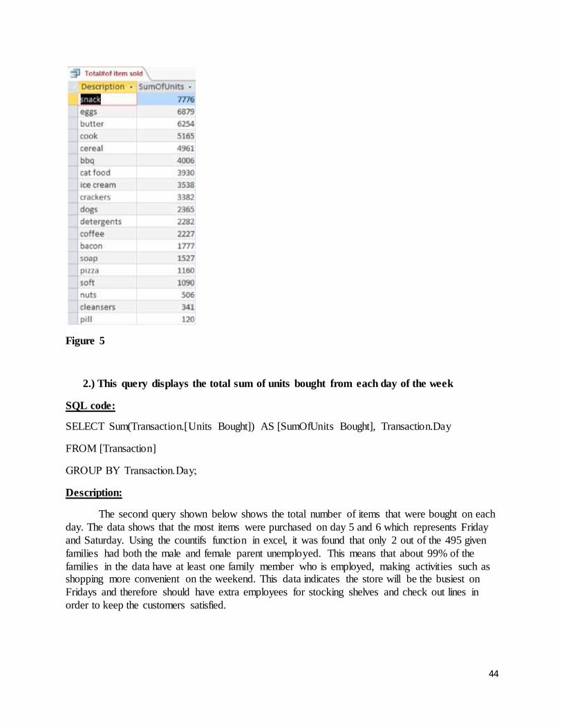
1.) This query displays the sum of the units bought for each item in descending order
SQL code:
SELECT ItemType.Description, Sum(Transaction.[Units Bought]) AS [SumOfUnits Bought]
FROM ItemType INNER JOIN [Transaction] ON ItemType.[Item Type] = Transaction.[Item Type]
GROUP BY ItemType.Description
ORDER BY Sum(Transaction.[Units Bought]) DESC;
Description:
The first query shown below is a calculation of the total number of units sold per item.
This table shows that snacks are the most sold item and pills are the least sold item. This
information is important to store management and vital for their success. It is important to have a
large enough inventory of these products to satisfy the customer demand. The placement of these products in the store can be important for advertisement purposes such as leading customers to
buy other products.
44
Figure 5
2.) This query displays the total sum of units bought from each day of the week
SQL code:
SELECT Sum(Transaction.[Units Bought]) AS [SumOfUnits Bought], Transaction.Day
FROM [Transaction]
GROUP BY Transaction.Day;
Description:
The second query shown below shows the total number of items that were bought on each
day. The data shows that the most items were purchased on day 5 and 6 which represents Friday
and Saturday. Using the countifs function in excel, it was found that only 2 out of the 495 given
families had both the male and female parent unemployed. This means that about 99% of the
families in the data have at least one family member who is employed, making activities such as shopping more convenient on the weekend. This data indicates the store will be the busiest on
Fridays and therefore should have extra employees for stocking shelves and check out lines in
order to keep the customers satisfied.

45
Figure 6
3.) This query counts the number of families of size 4, 5 and 6 with cable TV.
SQL code:
SELECT Count(Demographics.[Cable TV]) AS [CountOfCable TV], Demographics.[Family
Size]
FROM Demographics
GROUP BY Demographics.[Family Size], Demographics.[Cable TV], Demographics.[Family
Size]
HAVING (((Demographics.[Cable TV])=1) AND ((Demographics.[Family Size])>=4));
Figure 7
Description:
This query provides a count of families of size 4, 5 and 6 that have cable TV. The results
show that 16 families of 6 or more people, 24 families of 5 people and 59 families of 4 people
have cable TV. These totals refer strictly to the larger family size indicating that there is most
likely a variety of aged people living in the households. This information could be useful to
television marketers who are looking to attract a specific age range of people within these larger
families.
4.) This query displays the days of the week in descending order based upon when part
time (working less than 35 hours a week) women shop the most SQL code:

46
SELECT Transaction.Day, Sum(Transaction.[Units Bought]) AS [SumOfUnits Bought], Demographics.[Female Work Hours]
FROM CouponID INNER JOIN (Demographics INNER JOIN [Transaction] ON
Demographics.[Customer ID] = Transaction.[Custome ID]) ON CouponID.CouponID =
Transaction.CouponID
GROUP BY Transaction.Day, Demographics.[Female Work Hours]
HAVING (((Demographics.[Female Work Hours])=3))
ORDER BY Sum(Transaction.[Units Bought]) DESC;
Description:
The fourth query shown below shows the days of the week that the women who work part
time tend to shop on the most. The results show the majority of them tend to do their shopping
towards the end of the week, with the most shopping done on Saturdays. This is similar to the
results shown above in figure 6, which shows the most items being sold on Friday and Saturday. These results relate back to the importance of having extra staff on the weekends in order to keep
the customers satisfied and in and out of the store in a timely fashion.
Figure 8
5.) This query displays the days of the week in descending order based upon when part
time (working less than 35 hours a week) men shop the most
SQL code:
SELECT Transaction.Day, Sum(Transaction.[Units Bought]) AS [SumOfUnits Bought],
Demographics.[Male Work Hours] FROM Demographics INNER JOIN [Transaction] ON Demographics.[Customer ID] =
Transaction.[Custome ID]
GROUP BY Transaction.Day, Demographics.[Male Work Hours]

47
HAVING (((Demographics.[Male Work Hours])=3))
ORDER BY Sum(Transaction.[Units Bought]) DESC;
Description:
The fifth query shown below shows the days of the week that the men who work part time
tend to shop the most. The male work hours column that is equal to 2 refers back to the data dictionary which shows a value of 2 equaling work hours of less than 35 hours a week. The
results show that the majority of part time working men tend to do their shopping towards the end
of the week on days 5 and 6. In this regard, the data displays the same results as shown above for
part time working women. The analysis also showed the major difference in parttime working
males who shopped compared to women. As shown below in figure X, the most shopping was
done on day 6 by 366 male citizens in comparison with the 1750 female shoppers on day 6. This
information is important to the store owner because it tells them about the shopping crowd they
will be expecting.
Figure 9
6.) This query displays the top 5 customer ID’s of the people who purchased the most
ice cream
SQL code:
SELECT TOP 5 Transaction.[Custome ID], Transaction.[Item Type], Sum(Transaction.[Units Bought]) AS [SumOfUnits Bought]
FROM [Transaction]
GROUP BY Transaction.[Custome ID], Transaction.[Item Type]
HAVING (((Transaction.[Item Type])=13))
ORDER BY Sum(Transaction.[Units Bought]) DESC;

48
Description:
The sixth query shown below shows the top 5 customers that bought the most of item 13
which is ice cream. It shows the most ice cream bought by a single customer was equal to 90.
This information can be used to analyze specific demographic information about these customers
and to form any relationship among them that could increase sales in the future. This information
can be evaluated for any item and is also important for the distribution of coupons to increase the
chance of the best customer’s returning to the store. The customers will in turn be rewarded for
their top purchases.
Figure 10
7.) This query displays the items in order from the most to least purchased for
customers that make an income of $15,00$20,000.
SQL code:
SELECT Count(ItemType.[Item Type]) AS [CountOfItem Type], ItemType.Description,
Sum(Transaction.[Units Bought]) AS [SumOfUnits Bought], Demographics.Income
FROM ItemType INNER JOIN (Demographics INNER JOIN [Transaction] ON
Demographics.[Customer ID] = Transaction.[Custome ID]) ON ItemType.[Item Type] =
Transaction.[Item Type]
GROUP BY ItemType.Description, Demographics.Income
HAVING (((Demographics.Income)=4))
ORDER BY Sum(Transaction.[Units Bought]) DESC;

49
Figure 11 below shows the most purchased items by customers within the income range of 1520,000
Description:
The query number #7 shows The most purchased item by customers who make between
$15,000 and $20,000 is eggs, followed by snacks and butter. Furthermore, since the total number
of transactions for each item is fairly close to the total number of each item purchased, these
customers are more likely to only buy one item at a time. Encouraging “buying in bulk” by offering discounts when customers purchase more than one item could increase the number of
items bought per transaction.
8.) This query displays the number of items sold in order from highest to lowest for
customers with an income range of greater than $75,000
SQL Code:
SELECT Count(ItemType.[Item Type]) AS [CountOfItem Type], ItemType.Description,
Sum(Transaction.[Units Bought]) AS [SumOfUnits Bought], Demographics.Income
FROM ItemType INNER JOIN (Demographics INNER JOIN [Transaction] ON
Demographics.[Customer ID] = Transaction.[Custome ID]) ON ItemType.[Item Type] =
Transaction.[Item Type]
GROUP BY ItemType.Description, Demographics.Income
HAVING (((Demographics.Income)=11))
ORDER BY Sum(Transaction.[Units Bought]) DESC;
Description:

50
Query number 8 shows the most purchased item for customers with an income range greater than $75,000 is cat food. This information may be useful to analyze other important
demographic information about the customers in this income range such as number of pets. The
following top selling items are snacks, cereal and crackers which are common to all of the
income ranges. This shows that these common items are most likely immune to income
discrepancies and are purchased by a majority of the customers.
Figure 12 below shows the most purchased items by customers within the income range of
greater than 75,000
9.) This query displays the number of items sold in order from highest to lowest for
customers with an income range of $55,000$65,000.
SQL Code:
SELECT Count(ItemType.[Item Type]) AS [CountOfItem Type], ItemType.Description,
Sum(Transaction.[Units Bought]) AS [SumOfUnits Bought], Demographics.Income

51
FROM ItemType INNER JOIN (Demographics INNER JOIN [Transaction] ON
Demographics.[Customer ID] = Transaction.[Custome ID]) ON ItemType.[Item Type] =
Transaction.[Item Type]
GROUP BY ItemType.Description, Demographics.Income
HAVING (((Demographics.Income)=9))
ORDER BY Sum(Transaction.[Units Bought]) DESC;
Description:
As shown in Figure 13 below, for customers that make an income between
$55,00065,000 eggs were the top selling item followed by snacks and butter. These are common, everyday grocery items, the same that were observed to be purchased very frequently
by many other customer demographics, including lower income groups. This suggests that these
items may be immune to income discrepancies and are widely consumed by households within a
wide range of financial situations.
Figure 14
10.) This query displays the day of the week that retired women shop the most

52
SQL Code:
SELECT Transaction.Day, Count(Demographics.[Female Work Hours]) AS [CountOfFemale
Work Hours], Demographics.[Female Work Hours]
FROM Demographics INNER JOIN [Transaction] ON Demographics.[Customer ID] =
Transaction.[Custome ID]
GROUP BY Transaction.Day, Demographics.[Female Work Hours]
HAVING (((Demographics.[Female Work Hours])=4))
ORDER BY Count(Demographics.[Female Work Hours]) DESC;
Description:
The results below show that the majority of retired women shop on Fridays and Saturdays. This is similar to the shopping patterns found where it shows the most items are sold
at the store on Fridays and Saturdays.
11.) This query displays the days of the week that retired men shop the most
SQL Code:
SELECT Transaction.Day, Count(Demographics.[Male Work Hours]) AS [CountOfMale Work
Hours], Demographics.[Male Work Hours]
FROM Demographics INNER JOIN [Transaction] ON Demographics.[Customer ID] =
Transaction.[Custome ID]
GROUP BY Transaction.Day, Demographics.[Male Work Hours]
HAVING (((Demographics.[Male Work Hours])=4))
ORDER BY Count(Demographics.[Male Work Hours]) DESC;
Description:

53
The table below shows the days in which retired men go shopping the most in order from highest to lowest. The results show that the majority of retired men go shopping on Fridays
which is the same as the results of retired women.
12.) This query shows how the sales for one particular item, pizza, vary from
week to week. (Appendix 1)
SQL code:
SELECT Count(Transaction.[Item Type]) AS [CountOfItem Type], Transaction.Week,
Transaction.[Item Type]
FROM [Transaction]
GROUP BY Transaction.Week, Transaction.[Item Type], Transaction.[Item Type]
HAVING (((Transaction.[Item Type])=16))
ORDER BY Count(Transaction.[Item Type]) DESC;
Explanation:
This query showed how the sales of one particular item, in this case pizza, vary from
week to week. In this case, the sales don’t fluctuate too much among each other for any of the given weeks. The sales of pizza are pretty steady as shown which means there should be a
constant inventory of it in the store.
13.) This query shows an average of each unit bought for families with children.
An average value of units bought is given for values 18, which the data dictionary indicates
are all families with children. As expected, the numbers increase as the number of children
in the family increases. The results are shown in Appendix I. SQL Code:
SELECT Demographics.Children, Transaction.[Item Type], Avg(Transaction.[Units Bought])
AS [AvgOfUnits Bought]
FROM ItemType INNER JOIN (Demographics INNER JOIN [Transaction] ON

54
Demographics.[Customer ID] = Transaction.[Custome ID]) ON ItemType.[Item Type] = Transaction.[Item Type]
GROUP BY Demographics.Children, Transaction.[Item Type]
HAVING ((Not (Demographics.Children)=0));
14. This query shows the number of coupons and of what origin, that each ethnicity
used
SQL Code:
SELECT Demographics.Ethnicity, Count(CouponID.CouponOrigin) AS CountOfCouponOrigin,
CouponID.CouponOriginFROM ItemType INNER JOIN (Demographics INNER JOIN
(CouponID INNER JOIN [Transaction] ON CouponID.CouponID = Transaction.CouponID) ON
Demographics.[Customer ID] = Transaction.[Custome ID]) ON ItemType.[Item Type] =
Transaction.[Item Type]GROUP BY Demographics.Ethnicity, CouponID.CouponOrigin;
Description:

55
This query shows the number of coupons that each ethnicity used. As the data dictionary states the ethnicity value of 1 represents white people and coupon origin 19 represents ActNow.
As the figure above shows for example, there was one person from the white ethnic group that
used a coupon from ActNow. This information could be very important to the store owner in
order to target specific demographic areas with specific coupons. This information also shows
black people (ethnicity value 2) are the largest ethnic group that used zero coupons with 4271
people using zero. This information could also be useful to target these people with more
coupons and try to increase the store’s sales.
15. Top items that people of Ethnicity number 3 bought (Hispanic)
SQL Code:
SELECT ItemType.Description, Demographics.Ethnicity, Sum(Transaction.[Units Bought]) AS
[SumOfUnits Bought]
FROM ItemType INNER JOIN (Demographics INNER JOIN [Transaction] ON
Demographics.[Customer ID] = Transaction.[Custome ID]) ON ItemType.[Item Type] = Transaction.[Item Type]
GROUP BY ItemType.Description, Demographics.Ethnicity
HAVING (((Demographics.Ethnicity)=3))
ORDER BY Sum(Transaction.[Units Bought]) DESC;
Description:
The results shown below show that the top purchased item by people of ethnicity number
, which according to the data dictionary is Hispanic, was cereal which was followed by snacks
and detergents.

56
16. Top purchased items by ethnicity number 2 (Blacks)
SQL Code:
SELECT ItemType.Description, Demographics.Ethnicity, Sum(Transaction.[Units Bought]) AS
[SumOfUnits Bought]
FROM ItemType INNER JOIN (Demographics INNER JOIN [Transaction] ON
Demographics.[Customer ID] = Transaction.[Custome ID]) ON ItemType.[Item Type] = Transaction.[Item Type]
GROUP BY ItemType.Description, Demographics.Ethnicity
HAVING (((Demographics.Ethnicity)=2))
ORDER BY Sum(Transaction.[Units Bought]) DESC;
Description:
The results shown below show that the top purchased item by people of ethnicity number
2, which according to the data dictionary is Black, was eggs which was followed by snacks and
butter.

57
17.) This query displays the total number of items sold in the weeks of the summer
SQL Code:
SELECT ItemType.Description, Transaction.Week, Sum(Transaction.[Item Type]) AS
[SumOfItem Type]
FROM ItemType INNER JOIN [Transaction] ON ItemType.[Item Type] = Transaction.[Item Type]
WHERE (((Transaction.Week)>=26 And (Transaction.Week)<=38)) OR
(((Transaction.Week)>=78 And (Transaction.Week)<=90))
GROUP BY ItemType.Description, Transaction.Week
ORDER BY Transaction.Week, Sum(Transaction.[Item Type]) DESC;
Description:
This query shows that the customer’s buying behaviors are very similar to the buying
behaviours they exhibit throughout the rest of the year. The top selling item as shown below is
snacks which is common among all of the evaluations. The following top selling items are eggs,

o
58
crackers and ice cream. This informati n shows that it may be beneficial to the company to offer
sales on these items throughout the weeks of summer.
(rest displayed in access file!)
18.) This query displays the number of items sold in order from highest to lowest
for customers with an income range of greater than $45,000$55,000
SQL Code:
SELECT Count(ItemType.[Item Type]) AS [CountOfItem Type], ItemType.Description,

o
59
Sum(Transaction.[Units Bought]) AS [SumOfUnits Bought], Demographics.Income
FROM ItemType INNER JOIN (Dem graphics INNER JOIN [Transaction] ON
Demographics.[Customer ID] = Transaction.[Custome ID]) ON ItemType.[Item Type] =
Transaction.[Item Type]
GROUP BY ItemType.Description, Demographics.Income
HAVING (((Demographics.Income)=8))
ORDER BY Sum(Transaction.[Units Bought]) DESC;
Description:
Query 18 shows the top selling item for customers with an income range between
$45,000 and $55,000 was cat food followed by snacks, butter, eggs and cereal.
19.) This query shows the number of each item that was sold per day for days 17.

o
60
SQL Code:
SELECT Transaction.Day, ItemType.Description, Sum(Transaction.[Units Bought]) AS
[SumOfUnits Bought]
FROM ItemType INNER JOIN (Coup nID INNER JOIN [Transaction] ON
CouponID.CouponID = Transaction.CouponID) ON ItemType.[Item Type] = Transaction.[Item
Type]
GROUP BY Transaction.Day, ItemType.Description;
Description:
The results from query 18 shown below show the sum of each item purchased on days 17. For example as shown in figure X below, 181 units of bacon were purchased on Monday in
comparison to 193 units of bacon sold on Tuesday. The sum of units of ice cream bought
significantly increases on days 5 and 6 which is Friday and Saturday. This makes sense because
its the weekend and people will have a greater chance of wanting ice cream on weekends for
activities such as party’s etc. This variety in purchases shown can be important to store owners to
predict sales and inventory.

o
61

62
20. This query shows the top 5 items sold on day 6 (Saturday)
SQL code:
SELECT Top 5 Transaction.Day, ItemType.Description, Sum(Transaction.[Units Bought]) AS
[SumOfUnits Bought]
FROM ItemType INNER JOIN (CouponID INNER JOIN [Transaction] ON
CouponID.CouponID = Transaction.CouponID) ON ItemType.[Item Type] = Transaction.[Ite m Type]
GROUP BY Transaction.Day, ItemType.Description
HAVING (((Transaction.Day)=6))
ORDER BY Sum(Transaction.[Units Bought]) DESC;
Description:
As shown below in figure X, the top 5 items bought on Saturdays are snacks, eggs, butter,
cereal and cook. This information can be very important to store store owners to predict inventory
and sales. This information can also help in the planning of item sales which would draw in
additional customers to the store.
2.5 Discussion:
Once the database, queries and graphs were created, important trends were observed from the data. A summary of the data analysis is provided in 4 main categories
∙ Gender
∙ Income
∙ Week of the year
∙ Work hours
Work hours: The different work hours among the customers in the database were examined for any
potential buying patterns or trends. It was found that the most popular day to shop for part time men

63
and women was on Saturdays. Although the number of women part time shoppers greatly surpassed
the number of males with a count of 1750 compared to 366, it was found that both genders preferred to do their shopping on Saturdays.
As shown in query 10 and 11, the same calculation was done for retired males and females
and the results showed that the most popular day to shop for both genders was on Friday. In this
case, the amount of Friday shoppers for both male and females nearly doubled the Saturday
shoppers but Saturdays were still the second busiest day to shop. All of these results show that the
stores are the busiest on the weekends. This concept is very important for store managers to
recognize in order to have the proper staff on hand to keep customers happy and to have a fully
stocked inventory to avoid running out of items.
Gender
Specific trends related to gender were discovered when analyzing the queries our group
created, which lead us to many important conclusions. The female customers in the data bought a
much higher amount of items compared to men making them the bigger overall shoppers in the
database. From the given query results we can see the comparison between male and female part
time workers and their shopping habits (Units bought vs Hours of work). This particular example shows that in total on Saturday’s the women bought 1750 items while men just bought 366 items.
This difference in gender is surprisingly high.
The same pattern was not present when we analyzed the shopping patterns of retired males
and females. From the queries obtained we can observe that the retired men spent a similar
amount of time shopping as women and the total of their items bought were also very similar. In
other words, retired men shop as equal as retired female. We also found that the most frequent
day that retired individuals go shopping is on Friday and then Saturday. This may be the result of
some kind of sales that may occur in the shop on these days. The total number of items retired males bought on Fridays was 4232 in comparison to 4297 for retired females.
Income
After finalizing the queries and the results, the group came to the conclusion that
customers income did infact have a large influence on the customers buying behavior. At first
we can see from query #7 that customers with a low income, between $15,000$20,000 most
commonly bought item was eggs followed by snacks and butter. The count of the item purchased was also very close to the sum of units bought, indicating that the majority of these customers
buy each item one at time. One way to possibly increase these numbers is to increase the
coupons distributed for these items to these specific demographic regions.
As a commonality item among most of the data, item number 17 which was snacks
seemed to be the most popular. However, the most purchased item within each income range
differed slightly. From the lowest income group to the highest income group, the most frequently
purchased items were as follows: snacks, cat food, eggs, cereal, and cat food. Although the

a
64
distinct reason for these observations is not clear, more research may be beneficial to the store.
Knowing that these are the most frequently purchased items, management at the retail store could
make some rearrangements to the store layout. For example, they could place these items towards
the front of the store so that customers could find them easily, or they could place these items in
the back of the store so that customers would have to walk past many different items on their
way, and potentially buy some items that they weren’t looking for. Overall, customer income does have an affect on customer’s overall buying behavior at the store, both with the coupons
they use and the items they purchase.
Weeks of the year:
Another factor that was analyzed from the data was how the sales of certain items changed
from week to week. One of our queries (number 12), showed the different sales from one week to
another for item number 16 which was pizza. As the results given in Appendix I show, regardless
of season or week, the sales in pizza did not differ much from one another. There were one or two fluctuating weeks in the whole results but this fluctuation could have been a result of a birthday
party or another special occasion that happens once or twice a year. There were no major
fluctuations in pizza sales from one week to another.
The group also analyzed the top selling items in the weeks of the summer and it was found
that snacks were the highest selling item followed by eggs and crackers. These items are
commonality items that were found in many of our analysis as the top sellers. From one week to
another there were slight changes within the units of these items purchased but nothing drastic. This means that the store does not need to make any special preparations for the summer season
and can save money that may have been spent here and spend it elsewhere.
Figure A1: Sum of Units bought by day of the week
This pie chart shows the percentage of items bought by day. From this chart we can clearly
tell that the most sales occur on fridays and thursdays. This is very useful in determining when the

65
perfect day would be to restock the store. This information was obtained from a query created in
access showing the relation of the amount of items bought by each day.
Figure A2: Graphs showing Ice cream and Soft Drinks during the summer
The two graphs shown here were created by finding the relation of items sold during the summer. I then specifically selected Ice Cream and Soft Drinks as my 2 choices for comparison
because they both seem to have a similar pattern over the summer. For the most part they tend to have
similar spikes around the s me time periods of the 1st and 2nd summers. This information can help
stores prepare and plan their inventory for the these time periods to optimize sales.
Figure A3: Pie Chart of percentage of items sold by item type
This Pie chart can also help the stores prepare their stock. They can use this to rank how popular an item type is. The more popular the item type is, tells you that you should consider
having a wider range of this specific type. You can try stocking different flavors or different brands.

a
66
Also for the items that are not so popular, you can consider either advertising it better so that it sells
more, or even slowly decrease the amount of this item you stock on the shelves.
Figure A4: Graph of the Items most bought by people with Income 10 Stores should design their stores and inventory around the customers of the area. If there is
a vast number of a specific demographic for example this figure, taking the items that they mostly
buy can give insight on how to design your store around your customers. This idea optimizes
revenue and helps gain loyal customers.
Figure A5
These two pie charts show the percentage of items bought by males and females, respectively,
who work over 35 hours. Using this information you can better understand your customers needs
and cater to them. For example, since most males that work over 35 hrs shop on a wednesday, you

67
can then make small changes that would make the shop a more suitable environment for that
customer without losing the other customers interest completely.
Conclusion:
This project served as great practice in taking a large quantity of meaningless data,
analyzing, and then transforming it into meaningful information.The first part of the project was
used to see how reliable this data is. The calculations from the MAD and MSE show that this
data is in fact reliable. The method prefered would be the exponential smoothing with alpha=0.2
because the MAD values are lower for the ES than the 3pt moving average for both chosen items.
Also the TS was reasonably low so there also seemed to be very little bias. Many relationships
were established among the various categories of data in order to observe basic patterns and trends. The queries created in Access proved to be one of the most essential parts of this project.
The queries allowed the analyst to view only specific and desirable attributes of the data and
make conclusions about the data from these results. This also allows the analyst to obtain very
specific information bout the data and to observe how specific attributes interact with one
another.
Another crucial takeaway from this project is the importance of data visualization. The use
of various charts and graphics to display data makes patterns and trends a lot easier to interpret. In
conclusion, data analysis as a whole can be complicated but it is absolutely vital in order to make valuable and correct conclusions from large volumes of data.
Appendix I:
Table A1: 3 Point Moving average for cat food

a
68
Table A22: Exponential smoothing for cat food (alpha=0.2)
Figure A6: Graph Exponential Smoothing for cat food (alpha=0.2)
Table A3: 3 Point Moving average for cereal

69
Table A4: Exponential smoothing for cereal (alpha=0.2)
Figure A7: Graph Exponential Smoothing for cereal (alpha=0.2)

70
Full query results located in Access file

71
Roles
Wilson: Moving Average and Exponential Smoothing, Query graphs,
Jessica: Kmeans graphs and question 6 (open ended question), Queries and descriptions
Aaron: Regression, Queries and descriptions


