305
Ocean Engineering & Oceanography 5 Srinivasan Chandrasekaran Dynamic Analysis and Design of Offshore Structures

Ocean Engineering & Oceanography 5
Srinivasan Chandrasekaran
Dynamic Analysis and Design of Offshore Structures

Ocean Engineering & Oceanography
Volume 5
Series editors
Manhar R. Dhanak, Florida Atlantic University SeaTech, Dania Beach, USANikolas I. Xiros, New Orleans, USA

More information about this series at http://www.springer.com/series/10524

Srinivasan Chandrasekaran
Dynamic Analysisand Design of OffshoreStructures
123

Srinivasan ChandrasekaranDepartment of Ocean EngineeringIndian Institute of Technology MadrasChennai, Tamil NaduIndia
ISSN 2194-6396 ISSN 2194-640X (electronic)Ocean Engineering & OceanographyISBN 978-81-322-2276-7 ISBN 978-81-322-2277-4 (eBook)DOI 10.1007/978-81-322-2277-4
Library of Congress Control Number: 2015930819
Springer New Delhi Heidelberg New York Dordrecht London© Springer India 2015This work is subject to copyright. All rights are reserved by the Publisher, whether the whole or partof the material is concerned, specifically the rights of translation, reprinting, reuse of illustrations,recitation, broadcasting, reproduction on microfilms or in any other physical way, and transmissionor information storage and retrieval, electronic adaptation, computer software, or by similar ordissimilar methodology now known or hereafter developed.The use of general descriptive names, registered names, trademarks, service marks, etc. in thispublication does not imply, even in the absence of a specific statement, that such names are exemptfrom the relevant protective laws and regulations and therefore free for general use.The publisher, the authors and the editors are safe to assume that the advice and information in thisbook are believed to be true and accurate at the date of publication. Neither the publisher nor theauthors or the editors give a warranty, express or implied, with respect to the material containedherein or for any errors or omissions that may have been made.
Printed on acid-free paper
Springer (India) Pvt. Ltd. is part of Springer Science+Business Media (www.springer.com)

ToMy parents, teachers, family membersand friends

Preface
Offshore structures are unique in the field of engineering, as they pose manychallenges in the development and conceptualization of design. As innovativeplatform geometries are envisaged to alleviate the encountered environmental loadsefficiently, detailed understanding of their analysis and basic design becomesimportant. Structural dynamics, being an important domain of offshore engineering,require intensive teaching and guidance to illustrate the fundamental concepts, inparticular as applied to ocean structures. With the vast experience of teaching thissubject and guiding research, a humble attempt is made to present the basics in aclosed form, which will be useful for graduate students and researchers. Chapters inthis book are organized such that the reader gets an overall idea of various types ofoffshore plants, basic engineering requirements, fundamentals of structuraldynamics and their applications to preliminary design. Numerical examples andapplication problems are chosen to illustrate the use of experimental, numerical andanalytical studies in the design and development of new structural form for deep-water oil exploration. This book is an effort in the direction of capacity building ofpracticing and consulting offshore structural engineers who need to understand thebasic concepts of dynamic analysis of offshore structures through a simple andstraightforward approach.
Video lectures of the courses available at the following websites: (i) http://nptel.ac.in/courses/114106035; (ii) http://nptel.ac.in/courses/114106036; and (iii) http://nptel.ac.in/courses/114106037, which also substitute the classroom mode ofunderstanding of the contents of this book.
My sincere thanks are due to my professors, colleagues and my students whohave given their valuable input and feedback to develop the contents of this book.In particular, I wish to express my thanks to Mrs. Indira and Ms. Madhavi for theireditorial assistance and graphic art support extended during the preparation ofmanuscript of the book. Author acknowledges the support extended by Centre ofContinuing Education, Indian Institute of Technology Madras for publishing thisbook.
vii

I also owe a lot of thanks to all the authors and publishers who have earlierattempted to publish books on structural dynamics and allied topics, based on whichI developed my concepts on the said subject.
Srinivasan Chandrasekaran
viii Preface

Contents
1 Introduction to Offshore Platforms . . . . . . . . . . . . . . . . . . . . . . . 11.1 Introduction . . . . . . . . . . . . . . . . . . . . . . . . . . . . . . . . . . . 11.2 Types of Offshore Platforms. . . . . . . . . . . . . . . . . . . . . . . . 2
1.2.1 Bottom-supported Structures. . . . . . . . . . . . . . . . . . 31.2.2 Compliant Structures . . . . . . . . . . . . . . . . . . . . . . . 71.2.3 Floating Platform . . . . . . . . . . . . . . . . . . . . . . . . . 13
1.3 New-generation Offshore Platforms . . . . . . . . . . . . . . . . . . . 151.3.1 Buoyant Leg Structure (BLS) . . . . . . . . . . . . . . . . . 161.3.2 Triceratops . . . . . . . . . . . . . . . . . . . . . . . . . . . . . . 171.3.3 Floating, Storage and Regasification
Units (FSRUs) . . . . . . . . . . . . . . . . . . . . . . . . . . . 19
2 Environmental Forces . . . . . . . . . . . . . . . . . . . . . . . . . . . . . . . . . 252.1 Introduction . . . . . . . . . . . . . . . . . . . . . . . . . . . . . . . . . . . 252.2 Wind Force . . . . . . . . . . . . . . . . . . . . . . . . . . . . . . . . . . . 262.3 Wave Forces . . . . . . . . . . . . . . . . . . . . . . . . . . . . . . . . . . 302.4 Wave Theories . . . . . . . . . . . . . . . . . . . . . . . . . . . . . . . . . 312.5 Current Forces . . . . . . . . . . . . . . . . . . . . . . . . . . . . . . . . . 382.6 Earthquake Loads . . . . . . . . . . . . . . . . . . . . . . . . . . . . . . . 382.7 Ice and Snow Loads . . . . . . . . . . . . . . . . . . . . . . . . . . . . . 392.8 Marine Growth . . . . . . . . . . . . . . . . . . . . . . . . . . . . . . . . . 412.9 Mass . . . . . . . . . . . . . . . . . . . . . . . . . . . . . . . . . . . . . . . . 412.10 Damping . . . . . . . . . . . . . . . . . . . . . . . . . . . . . . . . . . . . . 422.11 Dead Load . . . . . . . . . . . . . . . . . . . . . . . . . . . . . . . . . . . . 422.12 Live Load . . . . . . . . . . . . . . . . . . . . . . . . . . . . . . . . . . . . 422.13 Impact Load . . . . . . . . . . . . . . . . . . . . . . . . . . . . . . . . . . . 432.14 General Design Requirements . . . . . . . . . . . . . . . . . . . . . . . 432.15 Steel Structures . . . . . . . . . . . . . . . . . . . . . . . . . . . . . . . . . 442.16 Allowable Stress Method . . . . . . . . . . . . . . . . . . . . . . . . . . 452.17 Limit State Method . . . . . . . . . . . . . . . . . . . . . . . . . . . . . . 452.18 Fabrication and Installation Loads . . . . . . . . . . . . . . . . . . . . 48
ix
2.19 Lifting Force . . . . . . . . . . . . . . . . . . . . . . . . . . . . . . . . . . 492.20 Load-Out Force . . . . . . . . . . . . . . . . . . . . . . . . . . . . . . . . 502.21 Transportation Forces . . . . . . . . . . . . . . . . . . . . . . . . . . . . 502.22 Launching and Upending Force . . . . . . . . . . . . . . . . . . . . . 532.23 Accidental Load . . . . . . . . . . . . . . . . . . . . . . . . . . . . . . . . 54
3 Introduction to Structural Dynamics . . . . . . . . . . . . . . . . . . . . . . 633.1 Introduction . . . . . . . . . . . . . . . . . . . . . . . . . . . . . . . . . . . 633.2 Fundamentals of Structural Dynamics . . . . . . . . . . . . . . . . . 643.3 Mathematical Model of Structural System . . . . . . . . . . . . . . 653.4 Single-Degree-of-Freedom Model . . . . . . . . . . . . . . . . . . . . 663.5 Equation of Motion . . . . . . . . . . . . . . . . . . . . . . . . . . . . . . 66
3.5.1 Simple Harmonic Motion Method (SHM Method). . . 673.5.2 Newton’s Law . . . . . . . . . . . . . . . . . . . . . . . . . . . 673.5.3 Energy Method. . . . . . . . . . . . . . . . . . . . . . . . . . . 683.5.4 Rayleigh’s Method . . . . . . . . . . . . . . . . . . . . . . . . 683.5.5 D’Alembert’s Principle . . . . . . . . . . . . . . . . . . . . . 69
3.6 Un-damped Free Vibration . . . . . . . . . . . . . . . . . . . . . . . . . 693.7 Damped Free Vibration . . . . . . . . . . . . . . . . . . . . . . . . . . . 70
3.7.1 Viscous Damping . . . . . . . . . . . . . . . . . . . . . . . . . 713.7.2 Coulomb Damping . . . . . . . . . . . . . . . . . . . . . . . . 723.7.3 Under-damped Systems . . . . . . . . . . . . . . . . . . . . . 743.7.4 Critically Damped Systems . . . . . . . . . . . . . . . . . . 753.7.5 Over-damped Systems . . . . . . . . . . . . . . . . . . . . . . 763.7.6 Half Power Method. . . . . . . . . . . . . . . . . . . . . . . . 77
3.8 Forced Vibration . . . . . . . . . . . . . . . . . . . . . . . . . . . . . . . . 783.8.1 Un-damped Forced Vibration . . . . . . . . . . . . . . . . . 793.8.2 Damped Forced Vibration . . . . . . . . . . . . . . . . . . . 80
3.9 Steady-State Response . . . . . . . . . . . . . . . . . . . . . . . . . . . . 823.10 Two-Degrees-of-Freedom Model . . . . . . . . . . . . . . . . . . . . . 833.11 Un-damped Free Vibrations and Principal
Modes of Vibration . . . . . . . . . . . . . . . . . . . . . . . . . . . . . . 843.12 Multi-degrees-of-Freedom . . . . . . . . . . . . . . . . . . . . . . . . . 893.13 Equation of Motion for Multi-degrees-of-Freedom System . . . 893.14 Influence Coefficients . . . . . . . . . . . . . . . . . . . . . . . . . . . . 913.15 Eigenvalue Problem. . . . . . . . . . . . . . . . . . . . . . . . . . . . . . 933.16 Dynamic Matrix Method . . . . . . . . . . . . . . . . . . . . . . . . . . 943.17 Dunkerley’s Method . . . . . . . . . . . . . . . . . . . . . . . . . . . . . 953.18 Matrix Iteration Method . . . . . . . . . . . . . . . . . . . . . . . . . . . 953.19 Stodola’s Method . . . . . . . . . . . . . . . . . . . . . . . . . . . . . . . 963.20 Mode Superposition Method. . . . . . . . . . . . . . . . . . . . . . . . 973.21 Mode Truncation . . . . . . . . . . . . . . . . . . . . . . . . . . . . . . . 98
3.21.1 Static Correction for Higher Mode Response . . . . . . 983.22 Rayleigh–Ritz Method—Analytical Approach . . . . . . . . . . . . 99
x Contents

4 Damping in Offshore Structures . . . . . . . . . . . . . . . . . . . . . . . . . 1554.1 Introduction . . . . . . . . . . . . . . . . . . . . . . . . . . . . . . . . . . . 1554.2 Damping Models: Rayleigh Damping . . . . . . . . . . . . . . . . . 157
4.2.1 Example Problem . . . . . . . . . . . . . . . . . . . . . . . . . 1604.3 Caughey Damping . . . . . . . . . . . . . . . . . . . . . . . . . . . . . . 161
4.3.1 Critical Problems Associatedwith Caughey Damping . . . . . . . . . . . . . . . . . . . . . 164
4.3.2 Example Problem . . . . . . . . . . . . . . . . . . . . . . . . . 1644.4 Classical Damping Matrix by Damping Matrix
Superpositioning . . . . . . . . . . . . . . . . . . . . . . . . . . . . . . . . 1664.4.1 Critical Issues . . . . . . . . . . . . . . . . . . . . . . . . . . . . 1674.4.2 Example Problem . . . . . . . . . . . . . . . . . . . . . . . . . 167
4.5 Evaluation of Damping from Experimental Results . . . . . . . . 169
5 Hydrodynamic Response of Perforated Offshore Members . . . . . . 1735.1 Fluid–Structure Interaction . . . . . . . . . . . . . . . . . . . . . . . . . 1735.2 Vertical Cylinders in Uniform Flow . . . . . . . . . . . . . . . . . . 1745.3 Flow in Deep Waters. . . . . . . . . . . . . . . . . . . . . . . . . . . . . 1745.4 Horizontal Cylinder in Uniform Flow . . . . . . . . . . . . . . . . . 1765.5 Horizontal Cylinder in Shear Flow . . . . . . . . . . . . . . . . . . . 1765.6 Blockage Factor . . . . . . . . . . . . . . . . . . . . . . . . . . . . . . . . 1765.7 Wave–Structure Interaction (WSI) . . . . . . . . . . . . . . . . . . . . 1775.8 Perforated Cylinders . . . . . . . . . . . . . . . . . . . . . . . . . . . . . 177
5.8.1 Wave Forces on Perforated Members. . . . . . . . . . . . 1775.8.2 Wave Forces on Offshore Structures
with Perforated Members . . . . . . . . . . . . . . . . . . . . 1795.8.3 Critical Review. . . . . . . . . . . . . . . . . . . . . . . . . . . 180
5.9 Experimental Investigations on Perforated Cylinders . . . . . . . 1815.10 Experimental Investigations on Perforated TLP Model . . . . . . 1855.11 Numerical Studies on Perforated Cylinders . . . . . . . . . . . . . . 189
5.11.1 Development of the Numerical Models . . . . . . . . . . 189
6 Introduction to Stochastic Dynamics . . . . . . . . . . . . . . . . . . . . . . 2036.1 Introduction . . . . . . . . . . . . . . . . . . . . . . . . . . . . . . . . . . . 203
6.1.1 Mean Value of the Response Process . . . . . . . . . . . 2056.2 Auto-Covariance of the Response Process . . . . . . . . . . . . . . 2076.3 Response Spectrum . . . . . . . . . . . . . . . . . . . . . . . . . . . . . . 2086.4 Stochastic Process . . . . . . . . . . . . . . . . . . . . . . . . . . . . . . . 210
6.4.1 Example of Stochastic Modeling . . . . . . . . . . . . . . . 2106.4.2 Example of a Stochastic Process . . . . . . . . . . . . . . . 211
6.5 Return Period . . . . . . . . . . . . . . . . . . . . . . . . . . . . . . . . . . 2126.6 Safety and Reliability . . . . . . . . . . . . . . . . . . . . . . . . . . . . 2136.7 Reliability Framework . . . . . . . . . . . . . . . . . . . . . . . . . . . . 213
Contents xi
6.8 Ultimate Limit State and Reliability Approach . . . . . . . . . . . 2156.9 Short-term Reliability of Single Load Effect . . . . . . . . . . . . . 216
6.9.1 Up-Crossing Approach . . . . . . . . . . . . . . . . . . . . . 2166.10 Long-term Reliability of Single Load Effect . . . . . . . . . . . . . 2186.11 Levels of Reliability . . . . . . . . . . . . . . . . . . . . . . . . . . . . . 2196.12 Reliability Methods . . . . . . . . . . . . . . . . . . . . . . . . . . . . . . 220
6.12.1 Advantages of Reliability Methods (ASC-83) . . . . . . 2206.13 Stochastic Models . . . . . . . . . . . . . . . . . . . . . . . . . . . . . . . 221
6.13.1 First-Order Second-Moment Method (FOSM) . . . . . . 2216.13.2 Advanced FOSM . . . . . . . . . . . . . . . . . . . . . . . . . 222
6.14 Fatigue and Fracture . . . . . . . . . . . . . . . . . . . . . . . . . . . . . 2246.15 Fatigue Assessment . . . . . . . . . . . . . . . . . . . . . . . . . . . . . . 225
6.15.1 SN Approach . . . . . . . . . . . . . . . . . . . . . . . . . . . . 2256.16 Miner’s Rule . . . . . . . . . . . . . . . . . . . . . . . . . . . . . . . . . . 2276.17 Fatigue Loading and Fatigue Analysis . . . . . . . . . . . . . . . . . 2286.18 Time Domain Fatigue Analysis . . . . . . . . . . . . . . . . . . . . . . 229
6.18.1 Rain Flow Counting . . . . . . . . . . . . . . . . . . . . . . . 2296.19 Deterministic Fatigue Analysis . . . . . . . . . . . . . . . . . . . . . . 2316.20 Spectral Fatigue Analysis . . . . . . . . . . . . . . . . . . . . . . . . . . 232
6.20.1 Narrowband Spectrum . . . . . . . . . . . . . . . . . . . . . . 2336.20.2 Broadband Spectrum . . . . . . . . . . . . . . . . . . . . . . . 234
6.21 Stress Concentration Factor (SCF). . . . . . . . . . . . . . . . . . . . 2386.22 Crack Propagation. . . . . . . . . . . . . . . . . . . . . . . . . . . . . . . 238
6.22.1 Step-by-Step Procedure to Compute the FatigueCrack Propagation. . . . . . . . . . . . . . . . . . . . . . . . . 239
7 Applications in Preliminary Analysis and Design . . . . . . . . . . . . . 2437.1 Free Vibration Response of Offshore Triceratops . . . . . . . . . 2437.2 New Structural Form . . . . . . . . . . . . . . . . . . . . . . . . . . . . . 2447.3 Model Details . . . . . . . . . . . . . . . . . . . . . . . . . . . . . . . . . . 2457.4 Experimental Studies . . . . . . . . . . . . . . . . . . . . . . . . . . . . . 247
7.4.1 Free-floating Studies . . . . . . . . . . . . . . . . . . . . . . . 2477.4.2 Free-decay Studies on Tethered Triceratops . . . . . . . 247
7.5 Analytical Studies . . . . . . . . . . . . . . . . . . . . . . . . . . . . . . . 2477.6 Empirical Prediction . . . . . . . . . . . . . . . . . . . . . . . . . . . . . 2497.7 Wave Directionality Effects on Offshore Triceratops . . . . . . . 2507.8 Discussions of Experimental Studies . . . . . . . . . . . . . . . . . . 2507.9 Springing and Ringing Responses of Tension
Leg Platforms . . . . . . . . . . . . . . . . . . . . . . . . . . . . . . . . . . 2567.9.1 Springing and Ringing. . . . . . . . . . . . . . . . . . . . . . 256
7.10 Evolution of Platform Geometry . . . . . . . . . . . . . . . . . . . . 2577.11 Mathematical Development . . . . . . . . . . . . . . . . . . . . . . . . 2587.12 Analytical Model of TLP . . . . . . . . . . . . . . . . . . . . . . . . . . 2597.13 Hydrodynamic Forces on TLP . . . . . . . . . . . . . . . . . . . . . . 262
xii Contents

7.14 Dynamics of Triangular TLP . . . . . . . . . . . . . . . . . . . . . . . 2637.14.1 Mass Matrix . . . . . . . . . . . . . . . . . . . . . . . . . . . . . 2637.14.2 Stiffness Matrix . . . . . . . . . . . . . . . . . . . . . . . . . . 2647.14.3 Damping Matrix . . . . . . . . . . . . . . . . . . . . . . . . . . 264
7.15 Ringing Response . . . . . . . . . . . . . . . . . . . . . . . . . . . . . . . 2657.16 Springing Response. . . . . . . . . . . . . . . . . . . . . . . . . . . . . . 2697.17 Significance of Springing and Ringing Response. . . . . . . . . . 273
References. . . . . . . . . . . . . . . . . . . . . . . . . . . . . . . . . . . . . . . . . . . . . 277
Index . . . . . . . . . . . . . . . . . . . . . . . . . . . . . . . . . . . . . . . . . . . . . . . . 285
Contents xiii
Figures
Fig. 1.1 Deep-water drilling semisubmersible with verticalriser storage . . . . . . . . . . . . . . . . . . . . . . . . . . . . . . . . . . 2
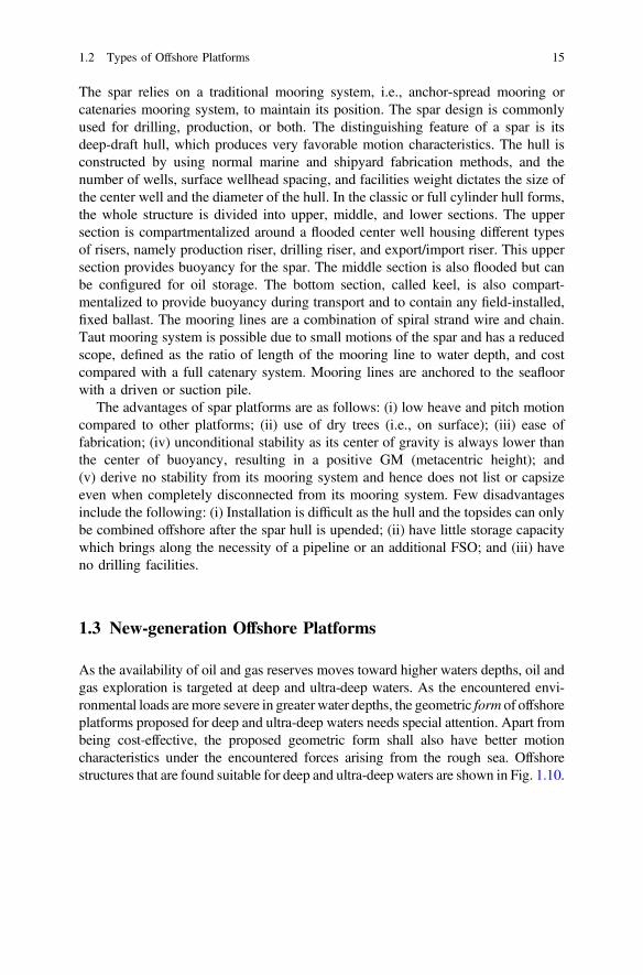
Fig. 1.2 Bullwinkle steel jacket . . . . . . . . . . . . . . . . . . . . . . . . . . . 5Fig. 1.3 Hibernia gravity base structure . . . . . . . . . . . . . . . . . . . . . 7Fig. 1.4 Lena guyed tower in Mississippi Canyon Block. . . . . . . . . . 9Fig. 1.5 Articulated tower . . . . . . . . . . . . . . . . . . . . . . . . . . . . . . . 10Fig. 1.6 Tension leg platform . . . . . . . . . . . . . . . . . . . . . . . . . . . . 10Fig. 1.7 Semisubmersible . . . . . . . . . . . . . . . . . . . . . . . . . . . . . . . 11Fig. 1.8 FPSO platform . . . . . . . . . . . . . . . . . . . . . . . . . . . . . . . . 11Fig. 1.9 SPAR platform . . . . . . . . . . . . . . . . . . . . . . . . . . . . . . . . 12Fig. 1.10 Different types of ultra-deep-water structures. . . . . . . . . . . . 16Fig. 1.11 Buoyant tower in the fabrication yard. . . . . . . . . . . . . . . . . 17Fig. 1.12 Load out and installed structure in offshore field . . . . . . . . . 18Fig. 1.13 Conceptual view of triceratops. . . . . . . . . . . . . . . . . . . . . . 18Fig. 2.1 Definition of wave parameters . . . . . . . . . . . . . . . . . . . . . . 32Fig. 2.2 Wave theory selection chart (Sarpakaya
and Issacson 1981). . . . . . . . . . . . . . . . . . . . . . . . . . . . . . 32Fig. 2.3 Bottom-supported cylinder . . . . . . . . . . . . . . . . . . . . . . . . 36Fig. 2.4 Lifts under different conditions. a Derrick and structure
on land. b Derrick on land, structure on floating barge.c Derrick and structure in the sea. . . . . . . . . . . . . . . . . . . . 49
Fig. 2.5 Different phases of jacket load-out by skidding . . . . . . . . . . 51Fig. 2.6 Motion of floating objects during installation . . . . . . . . . . . 52Fig. 2.7 View of launch barge and jacket undergoing motion . . . . . . 53Fig. 2.8 Launching and upending. . . . . . . . . . . . . . . . . . . . . . . . . . 53Fig. 3.1 Single-degree-of-freedom model . . . . . . . . . . . . . . . . . . . . 65Fig. 3.2 Free body diagram of single-degree-of-freedom model . . . . . 66Fig. 3.3 Un-damped free vibration of single-degree-of-freedom
model. . . . . . . . . . . . . . . . . . . . . . . . . . . . . . . . . . . . . . . 69Fig. 3.4 Damped free vibration of single-degree-of-freedom model. . . 71Fig. 3.5 Displacement of a system in coulomb damping . . . . . . . . . . 72Fig. 3.6 Response of under-damped system. . . . . . . . . . . . . . . . . . . 74Fig. 3.7 Response of critically damped system. . . . . . . . . . . . . . . . . 76
xv
Fig. 3.8 Response of over-damped system. . . . . . . . . . . . . . . . . . . . 77Fig. 3.9 Half power bandwidth method. . . . . . . . . . . . . . . . . . . . . . 78Fig. 3.10 Damped single degree of freedom under external
excitation . . . . . . . . . . . . . . . . . . . . . . . . . . . . . . . . . . . . 78Fig. 3.11 Steady-state response of damped single-degree-of-freedom
system . . . . . . . . . . . . . . . . . . . . . . . . . . . . . . . . . . . . . . 82Fig. 3.12 Variation of frequency ratio with phase angle for damped
vibration . . . . . . . . . . . . . . . . . . . . . . . . . . . . . . . . . . . . . 83Fig. 3.13 Variation of dynamic magnification factor with frequency
ratio for damped vibration. . . . . . . . . . . . . . . . . . . . . . . . . 83Fig. 3.14 Two-degrees-of-freedom system models. a Mass and
stiffness in series; b two pendulums connectedwith a bar of stiffness k . . . . . . . . . . . . . . . . . . . . . . . . . . 84
Fig. 3.15 Spring–mass un-damped two-degrees-of-freedom system. . . . 85Fig. 3.16 Un-damped multi-degrees-of-freedom model . . . . . . . . . . . . 91Fig. 4.1 Damping models a mass proportional damping
b stiffness proportional damping . . . . . . . . . . . . . . . . . . . . 157Fig. 4.2 Rayleigh damping . . . . . . . . . . . . . . . . . . . . . . . . . . . . . . 159Fig. 4.3 Example problem 4.2.1. . . . . . . . . . . . . . . . . . . . . . . . . . . 160Fig. 4.4 Example problem 4.3.2. . . . . . . . . . . . . . . . . . . . . . . . . . . 165Fig. 4.5 Example problem 4.4.2. . . . . . . . . . . . . . . . . . . . . . . . . . . 167Fig. 4.6 Free vibration experiment—heave acceleration
of model with perforated column . . . . . . . . . . . . . . . . . . . . 169Fig. 4.7 Free vibration experiment—surge acceleration of model
with perforated column. . . . . . . . . . . . . . . . . . . . . . . . . . . 169Fig. 5.1 Flow in deep waters . . . . . . . . . . . . . . . . . . . . . . . . . . . . . 175Fig. 5.2 Experimental setup to study response on perforated
cylinder . . . . . . . . . . . . . . . . . . . . . . . . . . . . . . . . . . . . . 181Fig. 5.3 Perforated cylinders considered for the study:
a inner cylinder; b outer cylinder (A); c outer cylinder (B);and d outer cylinder (C) . . . . . . . . . . . . . . . . . . . . . . . . . . 182
Fig. 5.4 Force variation in cylinders (WH = 5 cm). . . . . . . . . . . . . . 183Fig. 5.5 Force variation in cylinders (WH = 25 cm) . . . . . . . . . . . . . 184Fig. 5.6 Front view of TLP model: a without perforated cover;
b with perforated cover . . . . . . . . . . . . . . . . . . . . . . . . . . 185Fig. 5.7 Experimental setup: a components of the model;
b instrumentation . . . . . . . . . . . . . . . . . . . . . . . . . . . . . . . 186Fig. 5.8 Free surge acceleration with PC. . . . . . . . . . . . . . . . . . . . . 187Fig. 5.9 Free heave acceleration with PC . . . . . . . . . . . . . . . . . . . . 187Fig. 5.10 Surge RAO for 7-cm wave . . . . . . . . . . . . . . . . . . . . . . . . 188Fig. 5.11 Heave RAO for 7-cm wave. . . . . . . . . . . . . . . . . . . . . . . . 188Fig. 5.12 Tether tension variation for 7-cm wave. . . . . . . . . . . . . . . . 188Fig. 5.13 Perforated outer cylinder. . . . . . . . . . . . . . . . . . . . . . . . . . 189
xvi Figures
Fig. 5.14 Perforations along the circumference and length(Chandrasekaran et al. 2014) . . . . . . . . . . . . . . . . . . . . . . . 190
Fig. 5.15 Inner cylinder with perforated outer cylinder . . . . . . . . . . . . 190Fig. 5.16 Domain of inner cylinder generated with volumetric
control (Chandrasekaran et al. 2014) . . . . . . . . . . . . . . . . . 191Fig. 5.17 Domain of inner cylinder with perforated outer cylinder
generated with volumetric control(Chandrasekaran et al. 2014) . . . . . . . . . . . . . . . . . . . . . . . 191
Fig. 5.18 Simulation of inner cylinder (Chandrasekaran et al. 2014). . . 192Fig. 5.19 Simulation of inner cylinder with perforated outer cylinder
(Chandrasekaran et al. 2014) . . . . . . . . . . . . . . . . . . . . . . . 192Fig. 5.20 Force on inner cylinder (WH = 10 cm; WP = 1.6 s)
in numerical simulation . . . . . . . . . . . . . . . . . . . . . . . . . . 193Fig. 5.21 Force on inner cylinder with perforated outer cylinder
in numerical simulation (WH = 10 cm; WP = 1.6 s) . . . . . . 193Fig. 5.22 Comparison of forces on inner cylinder with and
without perforated outer cylinder . . . . . . . . . . . . . . . . . . . . 194Fig. 5.23 Horizontal velocity variation for various percentages
of perforation with wave steepness 0.0051 . . . . . . . . . . . . . 196Fig. 5.24 Horizontal velocity variation for various percentages
of perforation with wave steepness 0.0103 . . . . . . . . . . . . . 196Fig. 5.25 Horizontal velocity variation for various percentages
of perforation with wave steepness 0.0164 . . . . . . . . . . . . . 197Fig. 5.26 Horizontal velocity at mean sea level for various
wave steepness . . . . . . . . . . . . . . . . . . . . . . . . . . . . . . . . 198Fig. 5.27 Change in horizontal velocity between sections
and perforation ratio 11 %, and H/L 0.0962 . . . . . . . . . . . . 198Fig. 5.28 Change in horizontal velocity between sections
and steep wave . . . . . . . . . . . . . . . . . . . . . . . . . . . . . . . . 199Fig. 5.29 Change in horizontal velocity between sections
and medium steep wave . . . . . . . . . . . . . . . . . . . . . . . . . . 199Fig. 5.30 Change in horizontal velocity between section
and low-steep wave . . . . . . . . . . . . . . . . . . . . . . . . . . . . . 200Fig. 6.1 Amplitude amplification for various damping ratios . . . . . . . 210Fig. 6.2 Typical S–N curve . . . . . . . . . . . . . . . . . . . . . . . . . . . . . . 226Fig. 6.3 Spatial definition of notch, hot spot and surface
in a plane surface. . . . . . . . . . . . . . . . . . . . . . . . . . . . . . . 228Fig. 6.4 Hot spot stresses . . . . . . . . . . . . . . . . . . . . . . . . . . . . . . . 228Fig. 6.5 Example of rain flow counting . . . . . . . . . . . . . . . . . . . . . 230Fig. 7.1 Details of the scaled model . . . . . . . . . . . . . . . . . . . . . . . . 246Fig. 7.2 Model installed in the wave flume . . . . . . . . . . . . . . . . . . . 247Fig. 7.3 Analytical model of single BLS, free-floating triceratops,
and tethered triceratops. . . . . . . . . . . . . . . . . . . . . . . . . . . 248Fig. 7.4 Components of triceratops. . . . . . . . . . . . . . . . . . . . . . . . . 252
Figures xvii
Fig. 7.5 Plan and elevation of the scaled model . . . . . . . . . . . . . . . . 253Fig. 7.6 Instrumentation for different wave approach angles . . . . . . . 253Fig. 7.7 Surge/sway RAOs of triceratops . . . . . . . . . . . . . . . . . . . . 254Fig. 7.8 Heave RAOs of triceratops . . . . . . . . . . . . . . . . . . . . . . . . 254Fig. 7.9 Pitch/Roll RAOs of BLS . . . . . . . . . . . . . . . . . . . . . . . . . 255Fig. 7.10 Pitch/Roll RAO’s of deck . . . . . . . . . . . . . . . . . . . . . . . . . 255Fig. 7.11 Schematics of springing and ringing. . . . . . . . . . . . . . . . . . 256Fig. 7.12 Frequency range of TLPs relative to dominant
wave frequency . . . . . . . . . . . . . . . . . . . . . . . . . . . . . . . . 257Fig. 7.13 a PM spectrum for wave height elevation. b Impact wave
profile with impact wave at t = 10 s.c Non-impact wave profile . . . . . . . . . . . . . . . . . . . . . . . . 260
Fig. 7.14 a Plan and b elevation of example TLP . . . . . . . . . . . . . . . 261Fig. 7.15 Response of square TLPs to impact waves.
a Response of TLP1. b Response of TLP2.c Response of TLP3. d Response of TLP4. . . . . . . . . . . . . . 266
Fig. 7.16 Response of equivalent triangular TLPs to impact waves(T0 per tether same). a Response of TLP1. b Responseof TLP2. c Response of TLP3. d Response of TLP4 . . . . . . . 267
Fig. 7.17 Response of equivalent triangular TLPs to impact waves(total T0 same). a Response of TLP1. b Response of TLP2.c Response of TLP3. d Response of TLP4. . . . . . . . . . . . . . 268
Fig. 7.18 Response of square TLPs to non-impact waves.a Response of TLP1. b Response of TLP2.c Response of TLP3. d Response of TLP4. . . . . . . . . . . . . . 270
Fig. 7.19 Response of equivalent triangular TLPs to non-impact wave.a Response of TLP1. b Response of TLP2.c Response of TLP3. d Response of TLP4. . . . . . . . . . . . . . 271
Fig. 7.20 Response of equivalent triangular TLPs to non-impactwaves (total T0 same). a Response of TLP1.b Response of TLP2. c Response of TLP3.d Response of TLP4. . . . . . . . . . . . . . . . . . . . . . . . . . . . . 272
xviii Figures
Tables
Table 1.1 Offshore jacket platforms constructed worldwide . . . . . . . . . 4Table 1.2 Gravity platforms constructed worldwide
(Courtesy: Pennwell Publishing Co.) . . . . . . . . . . . . . . . . . . 6Table 2.1 Forces on members of different geometric shapes
using Froude–Krylov theory. . . . . . . . . . . . . . . . . . . . . . . . 37Table 2.2 Numerical values of C1–C4 . . . . . . . . . . . . . . . . . . . . . . . . 37Table 2.3 Typical live load values used in platform design
(Graff 1995). . . . . . . . . . . . . . . . . . . . . . . . . . . . . . . . . . . 43Table 2.4 Impact factor for live loads . . . . . . . . . . . . . . . . . . . . . . . . 43Table 2.5 Coefficient for resistance to stresses . . . . . . . . . . . . . . . . . . 45Table 2.6 Load factors . . . . . . . . . . . . . . . . . . . . . . . . . . . . . . . . . . . 45Table 2.7 Conditions specified for various limit states . . . . . . . . . . . . . 47Table 4.1 Results of free vibration experiment . . . . . . . . . . . . . . . . . . 170Table 5.1 Flow regimes in uniform flow . . . . . . . . . . . . . . . . . . . . . . 174Table 5.2 Reduced velocity range . . . . . . . . . . . . . . . . . . . . . . . . . . . 175Table 5.3 Geometric details of cylinders considered for the study . . . . . 182Table 5.4 Hydrodynamic forces for 25 cm wave height (N) . . . . . . . . . 183Table 5.5 Force reduction in inner cylinder . . . . . . . . . . . . . . . . . . . . 184Table 5.6 Details of TLP model . . . . . . . . . . . . . . . . . . . . . . . . . . . . 185Table 5.7 Comparison of mass of acrylic and aluminum
perforated covers . . . . . . . . . . . . . . . . . . . . . . . . . . . . . . . 186Table 5.8 Results of free-vibration experiment . . . . . . . . . . . . . . . . . . 187Table 5.9 Average surge response reduction . . . . . . . . . . . . . . . . . . . . 188Table 5.10 Details of cylinders . . . . . . . . . . . . . . . . . . . . . . . . . . . . . . 190Table 5.11 Details of perforations . . . . . . . . . . . . . . . . . . . . . . . . . . . . 190Table 5.12 Forces on inner cylinder (WH = 10 cm) . . . . . . . . . . . . . . . 194Table 5.13 Forces on inner cylinder with perforated
outer cylinder (WH = 10 cm) . . . . . . . . . . . . . . . . . . . . . . . 194Table 6.1 Merits and demerits of FOSM of reliability . . . . . . . . . . . . . 222Table 6.2 Rain flow counting . . . . . . . . . . . . . . . . . . . . . . . . . . . . . . 231Table 6.3 C conversion table . . . . . . . . . . . . . . . . . . . . . . . . . . . . . . 239Table 6.4 Fatigue crack propagation . . . . . . . . . . . . . . . . . . . . . . . . . 239
xix

Table 7.1 Mass properties of free-floating and tethered . . . . . . . . . . . . 245Table 7.2 Details of prototype and model of free-floating
and tethered triceratops . . . . . . . . . . . . . . . . . . . . . . . . . . . 246Table 7.3 Natural periods of the structure. . . . . . . . . . . . . . . . . . . . . . 249Table 7.4 Details of model and prototype of free-floating
and tethered triceratops . . . . . . . . . . . . . . . . . . . . . . . . . . . 251Table 7.5 Natural period of the structure(s) . . . . . . . . . . . . . . . . . . . . 252Table 7.6 Geometric properties of square TLPs considered . . . . . . . . . . 262Table 7.7 Natural wave periods and frequencies of equivalent
triangular TLPs with T0 per tether same. . . . . . . . . . . . . . . . 262Table 7.8 Values of coefficients for interpolation of Cm . . . . . . . . . . . . 262
xx Tables

Notations
qa Mass density of airCw Wind pressure coefficienth Phase anglev(t) Gust componentFD Drag forceFL Lift forcevz Wind speed at elevation of z m above MSLV10 Wind speed at 10 m above MSLFg Average gust factorLu Integral length scaleδ Surface drag coefficient/logarithmic decrementxp Peak frequencyr2z Variance of U(t)H Wave heightk Wave lengthd Water depthη Wave surface elevationk Wave numberx Wave circular frequencyf Cyclic frequencyq Density of fluidCd Drag coefficientsCm Inertia coefficientsDx Distance between the column membersS0 Intensity of earthquakexg Natural frequency of the groundng Damping of the ground�F0 Force amplitude on the structuref(t) Excitation force[k] Stiffness
xxi

[m] Mass element[c] Damping elementW Vertical loadx0 Initial displacements_x0 Initial velocitiesωn Natural frequencyA Areaµ Coefficient of absolute viscosityxd Damped vibration frequencyξ Damping ratioCc Critical dampingt Time periodpo Amplitude of varying load f(t)aij Flexibility influence coefficientx::
Accelerationm* Generalized massω* Generalized frequencyU/S UpstreamD/S DownstreamY Depth of immersionCBF Blockage factorS Center to center distance of the cylinderD Diameter of the cylinderT DraftFB Total buoyancya Area of perforationd Water depthg Acceleration due to gravityHFXðxÞ The transfer functionhFX(t) Impulse response functionCX(s) Auto-covarianceRX(s) Auto-correlationFm(m) Cumulative distribution function{fm(m)} Probability density functionPf Probability of failureHs Significant wave heightTp Spectral peak perioduc Current velocityuw Mean wave speedG(x) Performance functionβHL Reliability indexsg Stress range in each groupng Number of cycles in each groupDRC Fatigue damage estimated by range counting
xxii Notations

DRFC Rain flow countingDLCC Level crossing countingDPC Peak countingDNB Narrow band approximationng Number of cyclesD Total damageσ StressVCG Vertical center of gravityAw Water plane areaΔ DisplacementGMLa Lateral meta-centric heightsGMLo Longitudinal meta-centric heightsI Moment of InertiaRAO Response amplitude operator
Notations xxiii

About the Author
Srinivasan Chandrasekaran is a faculty member of the Department of OceanEngineering at Indian Institute of Technology Madras, Chennai, India. He hasteaching, research and industrial experience of about 23 years during which he hassupervised many sponsored research projects and offshore consultancy assignmentsboth in India and abroad. His areas of current research are dynamic analysis anddesign of offshore platforms, development of geometric forms of compliant offshorestructures for ultra-deep water oil exploration and production, sub-sea engineering,rehabilitation and retrofitting of offshore platforms, structural health monitoring ofocean structures, seismic analysis and design of structures and risk analyses, andreliability studies of offshore and petroleum engineering plants. He has also been avisiting fellow under the invitation of Ministry of Italian University Research toUniversity of Naples Federico II, Italy, for a period of 2 years during which heconducted research on advanced nonlinear modeling and analysis of structuresunder different environment loads with experimental verifications. He has published110 research papers in international journals and refereed conferences organized byprofessional societies around the world. He has also authored three textbooks whichare quite popular among graduate students of civil and ocean engineering. He is amember of many national and international professional bodies and delivered manyinvited lectures and keynote addresses in the international conferences, workshopsand seminars organized in India and abroad.
xxv
Chapter 1Introduction to Offshore Platforms
Abstract This chapter deals with the evolution of platform and various types ofoffshore platforms and their structural action under different environmental loads.The newly evolved structural forms and their discrete characteristics are discussedin this chapter. This chapter also gives the reader a good understanding about thestructural action of different forms in the offshore. An overview of the constructionstages of offshore plants and their foundation systems is presented.
Keywords Offshore structures � Bottom-supported structures � Compliantplatforms � Tension leg platforms � Triceratops � Floating � Storage and regasificationunit
1.1 Introduction
Offshore structures are being challenged to counteract the depletion of oil resourceswith the new set of discoveries. By 2010, the increase in drilling platforms inducedthe demand for offshore structures in deep sea. Hence, the quest on the research anddevelopment of the deep-water structures has resulted in the recent advancementand thrust in this area. Expansion of the structures from shallow to deep watersmakes the accessibility difficult, and hence, the structures demand higher deck areasconsisting of additional space for third-party drilling equipment. Specific challengesin Arctic regions in shallow waters that arise due to low temperature, remoteness,ice conditions, ecosystem, and safety necessitate an adaptive design of offshoreplatforms addressing these factors.
Development of offshore platforms depends on various factors:
• Structural geometry with a stable configuration• Easy to fabricate, install, and decommission• Low CAPEX• Early start of production• High return on investment by increased and uninterrupted production
© Springer India 2015S. Chandrasekaran, Dynamic Analysis and Design of Offshore Structures,Ocean Engineering & Oceanography 5, DOI 10.1007/978-81-322-2277-4_1
1
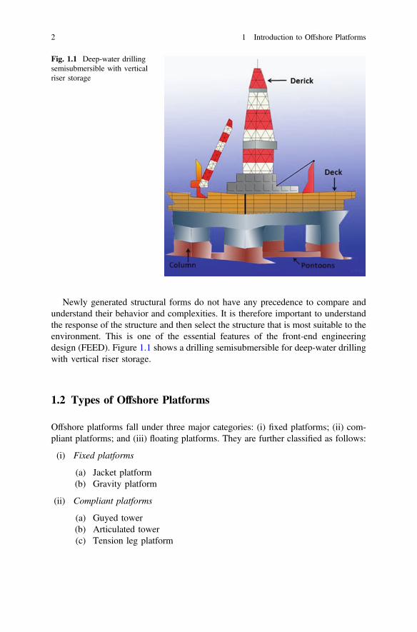
Newly generated structural forms do not have any precedence to compare andunderstand their behavior and complexities. It is therefore important to understandthe response of the structure and then select the structure that is most suitable to theenvironment. This is one of the essential features of the front-end engineeringdesign (FEED). Figure 1.1 shows a drilling semisubmersible for deep-water drillingwith vertical riser storage.
1.2 Types of Offshore Platforms
Offshore platforms fall under three major categories: (i) fixed platforms; (ii) com-pliant platforms; and (iii) floating platforms. They are further classified as follows:
(i) Fixed platforms
(a) Jacket platform(b) Gravity platform
(ii) Compliant platforms
(a) Guyed tower(b) Articulated tower(c) Tension leg platform
Fig. 1.1 Deep-water drillingsemisubmersible with verticalriser storage
2 1 Introduction to Offshore Platforms
(iii) Floating platforms
(a) Semisubmersible(b) Floating Production Unit (FPU)(c) Floating storage and offloading (FSO)(d) Floating production, storage and offloading (FPSO) System(e) Spar
1.2.1 Bottom-supported Structures
Energy is the driving force of the progress of civilization. Industrial advancementswere first stoked by coal and then by oil and gas. Oil and gas are essential com-modities in world trade. Oil exploration that initially started ashore has nowmoved tomuch deeper waters owing to the paucity of the resources at shallow waters (Bhat-tacharyya et al. 2003). Until date, there are more than 20,000 offshore platforms ofvarious kinds installed around the world. Geologists and geophysicists search for thepotential oil reserve within the ground under ocean seafloor, and engineers take theresponsibility of transporting the oil from the offshore site to the shore location(Dawson 1983). There are five major areas of operation from exploration to trans-portation of oil: (i) exploration; (ii) exploration drilling; (iii) development drilling;(iv) production operations; and (v) transportation (Chandrasekaran and Bhattachar-yya 2011; Clauss et al. 1992; Clauss and Birk 1996). Ever since the first offshorestructure was constructed, more advanced design technologies emerged for buildinglarger platforms that cater to deeper water requirements; each design is unique to thespecific site (Ertas and Eskwaro-Osire 1991). A precise classification of the offshoreplatform is difficult because of the large variety of parameters involved, such asfunctional aspects, geometric form, construction, and installation methods. However,the platforms are broadly classified based on the geometric configurations, in general(Chandrasekaran 2013a, b, c). Offshore installations are constructed for varied pur-poses: (i) exploratory and production drilling; (ii) preparing water or gas injectioninto reservoir; (iii) processing oil and gas; (iv) cleaning the produced oil for disposalinto sea; and (v) accommodation facilities. They are not classified on the basis of theirfunctional use but based on their geometric (structural) form (Sadehi 1989, 2001,2007; Sarpkaya and Isaacson 1981). As the platforms are aimed for greater waterdepths, their structural form changes significantly; alternatively, the same formcannot be used at a different water depth. It means that the geometric evolution of theplatform needs to be adaptive to counteract the environmental loads at the chosenwater depths (Patel 1989). Furthermore, the technological complexities faced by newoffshore platforms including analysis and design, topside details, construction, andinstallation are not available in the open domain; they are protected and owned by therespective companies/agencies as part of their copyright. Because of such practices,knowledge on the complexities in designing the offshore plants is not available to thepracticing young engineers, in particular. Hence, prior to the knowledge of FEED, it
1.2 Types of Offshore Platforms 3
is necessary to understand different structural forms of offshore structures, which aresuccessful in the past. As it is well known that each platform is unique in many ways,learning about their structural configurations, limitations with respect to the sea statesand water depth, construction complexities, decommissioning issues, and theirstructural action will be an important stage in the pre-FEED (Hsu 1981; Paik andThayamballi 2007).
The present trend is to design and install offshore platforms in regions that areinaccessible and difficult to use the existing technologies (Anagnostopoulos 1982).The structural form of every platform is largely derived on the basis of structuralinnovativeness but not on the basis of the functional advantages. Revisiting theexisting platforms constructed around the world will impart decent knowledge tooffshore engineers (Gerwick 1986; Graff 1981a, b). Offshore platforms are classi-fied either as bottom-supported or floating. Bottom-supported platforms can befurther classified as fixed or compliant-type structures; compliant means flexible(mobility). Compliancy changes the dynamic behavior of such platforms. Floatingstructures are classified as neutrally buoyant type (e.g., semisubmersibles, FPSO,mono-column spars) and positively buoyant type (e.g., tension leg platforms). It isimportant to note that buoyancy plays a very important role in floating-type offshorestructures, as the classifications are done based on buoyancy (Bea et al. 1999).Table 1.1 shows the list of jacket platforms constructed worldwide.
Fixed-type platforms are called template-type structures, which consist of thefollowing:
• A jacket or a welded space frame, which is designed to facilitate pile driving andalso acts as a lateral bracing for the piles
• Piles, which are permanently anchored to the seabed to resist the lateral andvertical loads that are transferred from the platform
• A superstructure consisting of the deck to support other operational activities
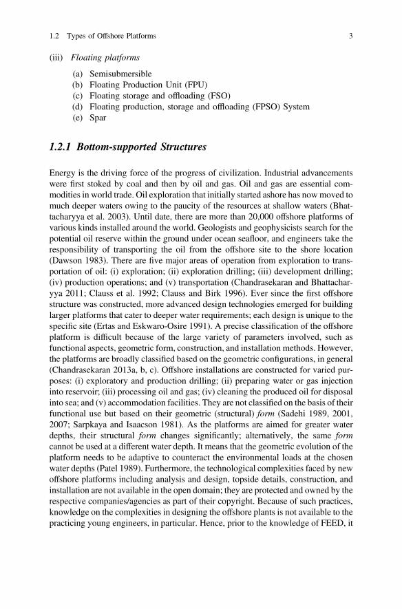
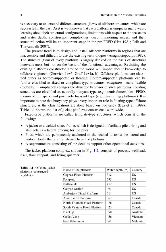
The jacket platform complex, shown in Fig. 1.2, consists of process, wellhead,riser, flare support, and living quarters.
Table 1.1 Offshore jacketplatforms constructedworldwide
Name of the platform Water depth (m) Country
Cognac Fixed Platform 312 US
Pompano 393 US
Bullwinkle 412 US
Canyon Station 91 US
Amberjack Fixed Platform 314 US
Alma Fixed Platform 67 Canada
North Triumph Fixed Platform 76 Canada
South Venture Fixed Platform 23 Canada
Blacktip 50 Australia
CaNguVang 56 Vietnam
East Belumut A 61 Malaysia
4 1 Introduction to Offshore Platforms
The advantages of offshore jacket platforms are as follows: (i) support large deckloads; (ii) possibility of being constructed in sections and transported; (iii) suitablefor large field and long-term production (supports a large number of wells);(iv) piles used for foundation result in good stability; and (v) not influenced byseafloor scour. Few disadvantages are as follows: (i) cost increases exponentiallywith increase in water depth; (ii) high initial and maintenance costs; (iii) notreusable; and (iv) steel structural members are subjected to corrosion, causingmaterial degradation in due course of service life.
1.2.1.1 Gravity Platform
In addition to steel jackets, concrete was also prominently used to build someoffshore structures. These structures are called gravity platforms or gravity-basedstructures (GBS). A gravity platform relies on the weight of the structure to resistthe encountered loads instead of piling (API-RP2A 1989). In regions where drivingpiles become difficult, structural forms are designed to lie on its own weight to resistthe environmental loads. These structures have foundation elements that contributesignificantly to the required weight and spread over a large area of the seafloor toprevent failure due to overturning moments caused by lateral loads. Gravity plat-forms are capable of supporting large topside loads during tow-out, which mini-mizes the hookup work during installation. Additional large storage spaces forhydrocarbons add up to their advantage. Their salient advantages include the fol-lowing: (i) constructed onshore and transported; (ii) towed to the site of installation;(iii) quick installation by flooding; and (iv) use of traditional methods and labor forinstallation. Table 1.2 shows the list of gravity platforms constructed worldwide.These platforms are also known to be responsible for seabed scouring due to largefoundations, causing severe environmental impact (Chandrasekaran 2013a).
Gravity platforms had serious limitations, namely (i) not suitable for sites of poorsoil conditions, as this would lead to significant settlement of foundation; (ii) long
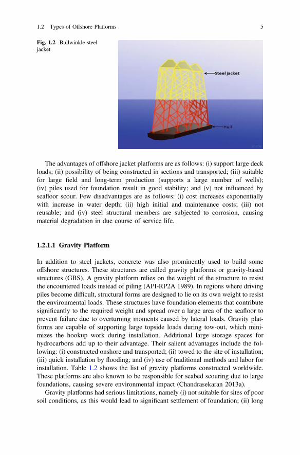
Fig. 1.2 Bullwinkle steeljacket
1.2 Types of Offshore Platforms 5
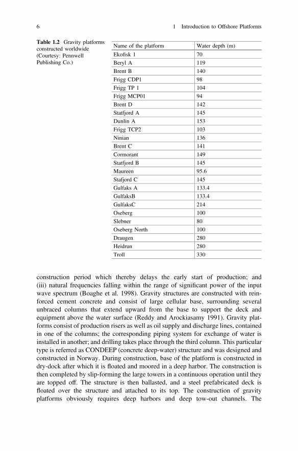
construction period which thereby delays the early start of production; and(iii) natural frequencies falling within the range of significant power of the inputwave spectrum (Boaghe et al. 1998). Gravity structures are constructed with rein-forced cement concrete and consist of large cellular base, surrounding severalunbraced columns that extend upward from the base to support the deck andequipment above the water surface (Reddy and Arockiasamy 1991). Gravity plat-forms consist of production risers as well as oil supply and discharge lines, containedin one of the columns; the corresponding piping system for exchange of water isinstalled in another; and drilling takes place through the third column. This particulartype is referred as CONDEEP (concrete deep-water) structure and was designed andconstructed in Norway. During construction, base of the platform is constructed indry-dock after which it is floated and moored in a deep harbor. The construction isthen completed by slip-forming the large towers in a continuous operation until theyare topped off. The structure is then ballasted, and a steel prefabricated deck isfloated over the structure and attached to its top. The construction of gravityplatforms obviously requires deep harbors and deep tow-out channels. The
Table 1.2 Gravity platformsconstructed worldwide(Courtesy: PennwellPublishing Co.)
Name of the platform Water depth (m)
Ekofisk 1 70
Beryl A 119
Brent B 140
Frigg CDP1 98
Frigg TP 1 104
Frigg MCP01 94
Brent D 142
Statfjord A 145
Dunlin A 153
Frigg TCP2 103
Ninian 136
Brent C 141
Cormorant 149
Statfjord B 145
Maureen 95.6
Stafjord C 145
Gulfaks A 133.4
GulfaksB 133.4
GulfaksC 214
Oseberg 100
Slebner 80
Oseberg North 100
Draugen 280
Heidrun 280
Troll 330
6 1 Introduction to Offshore Platforms
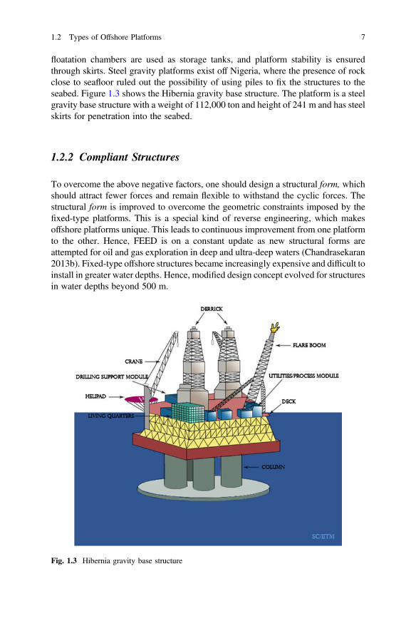
floatation chambers are used as storage tanks, and platform stability is ensuredthrough skirts. Steel gravity platforms exist off Nigeria, where the presence of rockclose to seafloor ruled out the possibility of using piles to fix the structures to theseabed. Figure 1.3 shows the Hibernia gravity base structure. The platform is a steelgravity base structure with a weight of 112,000 ton and height of 241 m and has steelskirts for penetration into the seabed.
1.2.2 Compliant Structures
To overcome the above negative factors, one should design a structural form, whichshould attract fewer forces and remain flexible to withstand the cyclic forces. Thestructural form is improved to overcome the geometric constraints imposed by thefixed-type platforms. This is a special kind of reverse engineering, which makesoffshore platforms unique. This leads to continuous improvement from one platformto the other. Hence, FEED is on a constant update as new structural forms areattempted for oil and gas exploration in deep and ultra-deep waters (Chandrasekaran2013b). Fixed-type offshore structures became increasingly expensive and difficult toinstall in greater water depths. Hence, modified design concept evolved for structuresin water depths beyond 500 m.
Fig. 1.3 Hibernia gravity base structure
1.2 Types of Offshore Platforms 7
A compliant tower is similar to that of a traditional platform, which extends fromsurface to the sea bottom and transparent to waves. A compliant tower is designed toremain flexible (adaptive) with the forces of waves, wind, and current. Classificationunder compliant structure includes those structures that extend to the ocean bottomand are anchored directly to the seafloor by piles and/or guidelines (Mather 2000).Guyed towers, articulated tower and tension leg platform (TLP) fall under this cate-gory. The structural action of complaint platforms is significantly different from thatof the fixed ones, as they resist lateral loads not by their weight but by their relativemovement. In fact, instead of resisting the lateral loads, the structural geometryenables the platform to move in line with the wave forces. To facilitate the productionoperation, they are position-restrained by cables/tethers or guy wires. By attachingthe wires to the complaint tower, majority of the lateral loads are counteracted by thehorizontal component of the tension in the cables; the vertical component adds to theweight and improves stability (Chakrabarti 1994; Dawson 1983).
1.2.2.1 Guyed Towers
Guyed tower is a slender structure made up of truss members that rest on the oceanfloor and is held in place by a symmetric array of catenary guylines. The foundationof the tower is supported with the help of spud can arrangement, which is similar tothe inverted cone placed under suction. The structural action of the guyed towermakes its innovation more interesting, which is one of the successful formimprovements in the offshore structural design. The upper part of the guy wire is alead cable, which acts as a stiff spring in moderate seas. The lower portion is aheavy chain, which is attached with clump weights. Under normal operating con-ditions, the weights will remain at the bottom, and the tower-deck motion will benearly insignificant. However, during a severe storm, the weights on the storm-wardside will lift off the bottom, softening the guying system and permitting the towerand guying system to absorb the large wave loads. Since the guylines are attachedto the tower below mean water level close to the center of applied environmentalforces, large overturning moments will not be transmitted through the structure tothe base. This feature has evolved in the design of the tower to be of a constantsquare cross section along its length, reducing the structural steel weight as com-pared with that of a conventional platform (Moe and Verley 1980).
Exxon in 1983 installed the first guyed tower named Lena guyed tower in theMississippi Canyon Block in a 300 m water depth. Though the structural formresembles a jacket structure, it is compliant and is moored by catenary anchor lines.The tower has a natural period of 28 s in sway mode while bending, and torsionmodes have a period of 3.9 and 5.7 s, respectively. The tower consists of 12buoyancy tanks of diameter 6 m and length of about 35 m. Around 20 guylines areattached to the tower with clump weights of about 180 ton to facilitate the holdingof the tower in position. The advantages of guyed towers are (i) low cost (lowerthan steel jacket); (ii) good stability as guylines and clump weights improverestoring force; and (iii) possible reuse. The disadvantages are as follows: (i) high
8 1 Introduction to Offshore Platforms
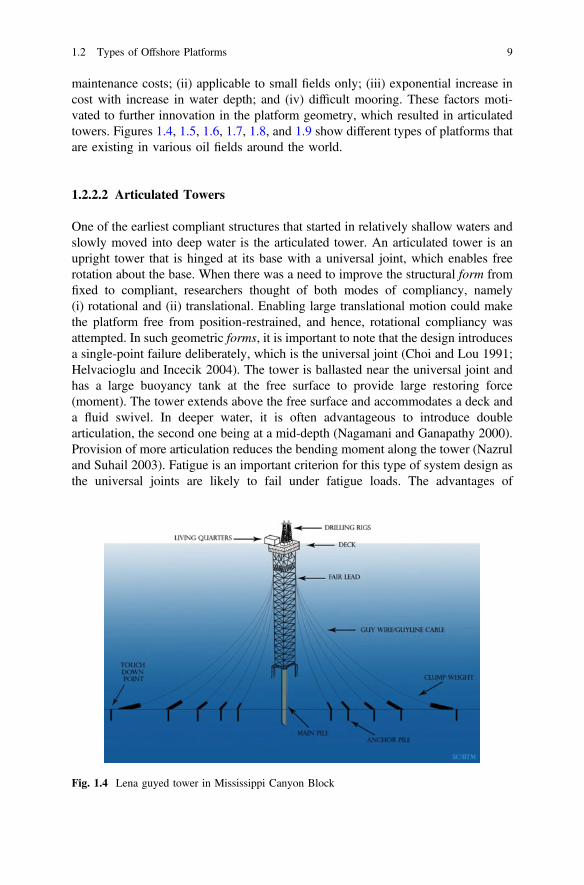
maintenance costs; (ii) applicable to small fields only; (iii) exponential increase incost with increase in water depth; and (iv) difficult mooring. These factors moti-vated to further innovation in the platform geometry, which resulted in articulatedtowers. Figures 1.4, 1.5, 1.6, 1.7, 1.8, and 1.9 show different types of platforms thatare existing in various oil fields around the world.
1.2.2.2 Articulated Towers
One of the earliest compliant structures that started in relatively shallow waters andslowly moved into deep water is the articulated tower. An articulated tower is anupright tower that is hinged at its base with a universal joint, which enables freerotation about the base. When there was a need to improve the structural form fromfixed to compliant, researchers thought of both modes of compliancy, namely(i) rotational and (ii) translational. Enabling large translational motion could makethe platform free from position-restrained, and hence, rotational compliancy wasattempted. In such geometric forms, it is important to note that the design introducesa single-point failure deliberately, which is the universal joint (Choi and Lou 1991;Helvacioglu and Incecik 2004). The tower is ballasted near the universal joint andhas a large buoyancy tank at the free surface to provide large restoring force(moment). The tower extends above the free surface and accommodates a deck anda fluid swivel. In deeper water, it is often advantageous to introduce doublearticulation, the second one being at a mid-depth (Nagamani and Ganapathy 2000).Provision of more articulation reduces the bending moment along the tower (Nazruland Suhail 2003). Fatigue is an important criterion for this type of system design asthe universal joints are likely to fail under fatigue loads. The advantages of
Fig. 1.4 Lena guyed tower in Mississippi Canyon Block
1.2 Types of Offshore Platforms 9
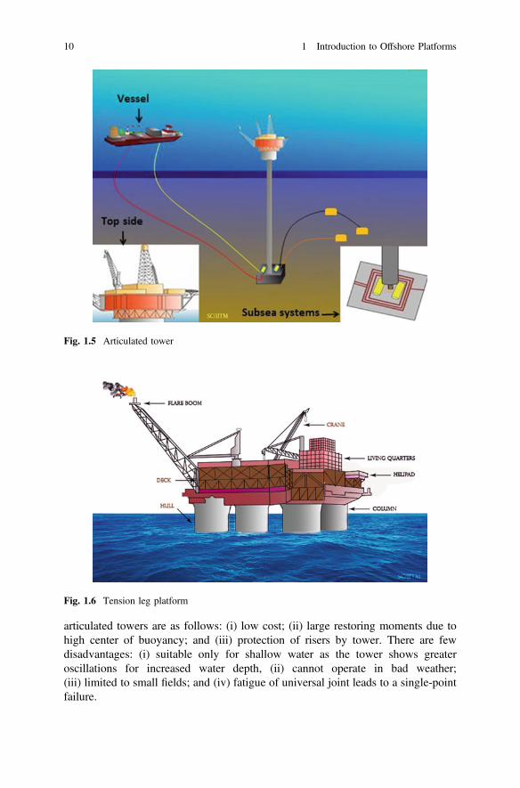
articulated towers are as follows: (i) low cost; (ii) large restoring moments due tohigh center of buoyancy; and (iii) protection of risers by tower. There are fewdisadvantages: (i) suitable only for shallow water as the tower shows greateroscillations for increased water depth, (ii) cannot operate in bad weather;(iii) limited to small fields; and (iv) fatigue of universal joint leads to a single-pointfailure.
Fig. 1.5 Articulated tower
Fig. 1.6 Tension leg platform
10 1 Introduction to Offshore Platforms
In both the above structural forms of complaint towers, it is seen that thestructure (tower) extends through the water depth, making it expensive for deepwaters. Therefore, successive structural forms are motivated toward the basicconcept of not extending the tower to the full water depth but only to retain it nearthe free surface level. In such kinds of structural geometry, it is inevitable to makethe platform weight dominant. To improve the installing features and decommis-sioning procedures, the geometry is attempted to be buoyancy dominant instead of
Fig. 1.7 Semisubmersible
Fig. 1.8 FPSO platform
1.2 Types of Offshore Platforms 11
weight dominant (buoyancy force exceeds the weight by manifold). While thisenabled easy fabrication and installation, it also demanded skilled labor and highexpertise for installation and commissioning of such platforms. The evolvedstructural geometry is TLPs (Vannucci 1996; de Boom et al. 1984; Yan et al. 2009;Yoneya and Yoshida 1982; Demirbilek 1990).
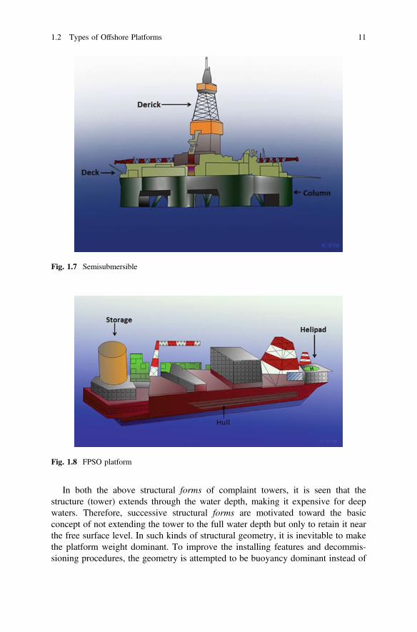
1.2.2.3 Tension Leg Platform
A TLP is a vertically moored compliant platform. Taut mooring lines verticallymoor the floating platform, with its excess buoyancy; they are called tendons ortethers. The structure is vertically restrained, while it is compliant in the horizontaldirection, which permits surge, sway, and yaw motions. The structural actionresulted in low vertical force in rough seas, which is the key design factor(Chandrasekaran and Jain 2002a, b; Rijken et al. 1991). Substantial pretension isrequired to prevent the tendons from falling slack even in the deepest trough, whichis achieved by increasing the free-floating draft (Chandrasekaran et al. 2006b).Typical natural periods of the TLP are kept away from the range of wave excitationperiods and typically for TLP resonance periods of 132 s (surge/sway) and 92 s(yaw) as well as 3.1 s (heave) and 3.5 s (pitch/roll), which are achieved throughproper design (Nordgren 1987). The main challenge for the TLP designers is tokeep the natural periods in heave and pitch below the range of significant waveenergy, which is achieved by an improved structural form (Paik and Roesset 1996;Kobayashi et al. 1987; Low 2009). TLP technology preserves many of the
Fig. 1.9 SPAR platform
12 1 Introduction to Offshore Platforms
operational advantages of a fixed platform while reducing the cost of production inwater depths up to about 1,500 m (Iwaski 1981; Haritos 1985; Chandrasekaranet al. 2004, 2007a; Chandrasekaran and Jain 2004). Its production and maintenanceoperations are similar to those of fixed platforms. TLPs are weight sensitive buthave limitations in accommodating heavy payloads (Tabeshpour et al. 2006;Yoshida et al. 1984). Usually, a TLP is fabricated and towed to an offshore well sitewherein the tendons are already installed on a prepared seabed. Then, the TLP isballasted down so that the tendons may be attached to the TLP at its four corners.The mode of transportation of TLP allows the deck to be joined to the TLP atdockside before the hull is taken offshore (Bar-Avi 1999).
The advantages of TLPS are as follows: (i) mobile and reusable; (ii) stable as theplatform has minimal vertical motion; (iii) low increase in cost with increase in waterdepth; (iv) deep-water capability; and (v) low maintenance cost. Few disadvantagesare, namely (i) high initial cost; (ii) high subsea cost; (iii) fatigue of tension legs;(iv) difficult maintenance of subsea systems; and (v) little or no storage.
1.2.3 Floating Platform
Semisubmersibles, FPSO systems, FPUs, FSO systems, and spar platforms aregrouped under this category.
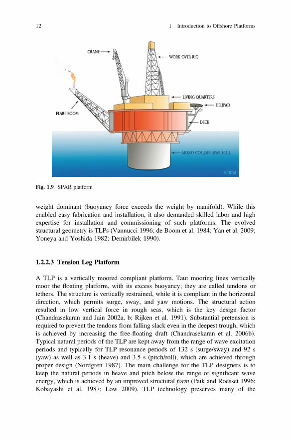
1.2.3.1 Semisubmersible
Semisubmersible marine structures are well known in the oil and gas industries andbelong to the category of neutrally buoyant structure. These structures are typicallymoveable only by towing. These semisubmersibles have a relatively low transitdraft, with a large water plane area, which allows them to be floated to a stationinglocation. On location, it is ballasted, usually by seawater, to assume a relativelydeep draft or semisubmerged condition, with a smaller water plane area, foroperation. Semisubmersible platforms have the principal characteristic of remainingin a substantially stable position and have minimal motions in all the degrees offreedom due to environmental forces such as the wind, waves, and currents. Themain parts of the semisubmersibles are the pontoons, columns, deck, and themooring lines. The columns bridge the deck and the pontoons, i.e., the deck issupported by columns. Flotation of semisubmersibles is accomplished with pon-toons. The pontoons provide a relatively large water plane area, as is desirable fortransit. When submerged for stationing and operations, the columns connecting thepontoons to the upper deck present a lower water plane area, thereby attracting lesswave loads and thus reducing the motions.
The advantages of semisubmersibles are as follows: (i) mobility with high transitspeed (*10kts); (ii) stable as they showminimal response towave action; and (iii) largedeck area. Few disadvantages are as follows: (i) high initial and operating costs;
1.2 Types of Offshore Platforms 13
(ii) limited deck load (low reserve buoyancy); (iii) structural fatigue; (iv) expensive tomove large distances; (v) availability of limited dry-docking facilities; and (vi) difficultto handle mooring systems and land BOP stack and riser in rough seas.
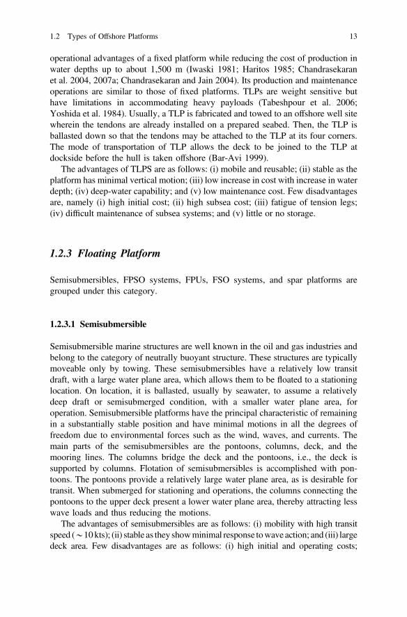
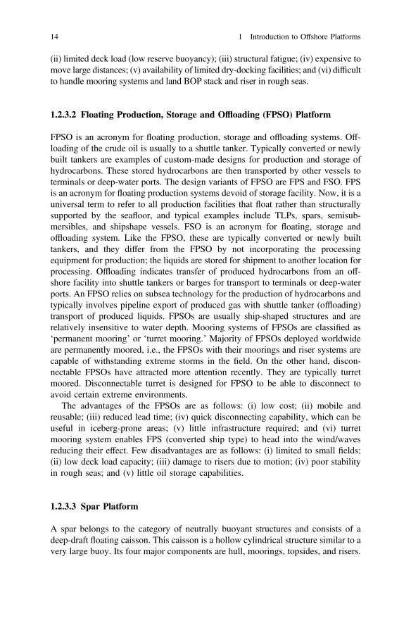
1.2.3.2 Floating Production, Storage and Offloading (FPSO) Platform
FPSO is an acronym for floating production, storage and offloading systems. Off-loading of the crude oil is usually to a shuttle tanker. Typically converted or newlybuilt tankers are examples of custom-made designs for production and storage ofhydrocarbons. These stored hydrocarbons are then transported by other vessels toterminals or deep-water ports. The design variants of FPSO are FPS and FSO. FPSis an acronym for floating production systems devoid of storage facility. Now, it is auniversal term to refer to all production facilities that float rather than structurallysupported by the seafloor, and typical examples include TLPs, spars, semisub-mersibles, and shipshape vessels. FSO is an acronym for floating, storage andoffloading system. Like the FPSO, these are typically converted or newly builttankers, and they differ from the FPSO by not incorporating the processingequipment for production; the liquids are stored for shipment to another location forprocessing. Offloading indicates transfer of produced hydrocarbons from an off-shore facility into shuttle tankers or barges for transport to terminals or deep-waterports. An FPSO relies on subsea technology for the production of hydrocarbons andtypically involves pipeline export of produced gas with shuttle tanker (offloading)transport of produced liquids. FPSOs are usually ship-shaped structures and arerelatively insensitive to water depth. Mooring systems of FPSOs are classified as‘permanent mooring’ or ‘turret mooring.’ Majority of FPSOs deployed worldwideare permanently moored, i.e., the FPSOs with their moorings and riser systems arecapable of withstanding extreme storms in the field. On the other hand, discon-nectable FPSOs have attracted more attention recently. They are typically turretmoored. Disconnectable turret is designed for FPSO to be able to disconnect toavoid certain extreme environments.
The advantages of the FPSOs are as follows: (i) low cost; (ii) mobile andreusable; (iii) reduced lead time; (iv) quick disconnecting capability, which can beuseful in iceberg-prone areas; (v) little infrastructure required; and (vi) turretmooring system enables FPS (converted ship type) to head into the wind/wavesreducing their effect. Few disadvantages are as follows: (i) limited to small fields;(ii) low deck load capacity; (iii) damage to risers due to motion; (iv) poor stabilityin rough seas; and (v) little oil storage capabilities.
1.2.3.3 Spar Platform
A spar belongs to the category of neutrally buoyant structures and consists of adeep-draft floating caisson. This caisson is a hollow cylindrical structure similar to avery large buoy. Its four major components are hull, moorings, topsides, and risers.
14 1 Introduction to Offshore Platforms
The spar relies on a traditional mooring system, i.e., anchor-spread mooring orcatenaries mooring system, to maintain its position. The spar design is commonlyused for drilling, production, or both. The distinguishing feature of a spar is itsdeep-draft hull, which produces very favorable motion characteristics. The hull isconstructed by using normal marine and shipyard fabrication methods, and thenumber of wells, surface wellhead spacing, and facilities weight dictates the size ofthe center well and the diameter of the hull. In the classic or full cylinder hull forms,the whole structure is divided into upper, middle, and lower sections. The uppersection is compartmentalized around a flooded center well housing different typesof risers, namely production riser, drilling riser, and export/import riser. This uppersection provides buoyancy for the spar. The middle section is also flooded but canbe configured for oil storage. The bottom section, called keel, is also compart-mentalized to provide buoyancy during transport and to contain any field-installed,fixed ballast. The mooring lines are a combination of spiral strand wire and chain.Taut mooring system is possible due to small motions of the spar and has a reducedscope, defined as the ratio of length of the mooring line to water depth, and costcompared with a full catenary system. Mooring lines are anchored to the seafloorwith a driven or suction pile.
The advantages of spar platforms are as follows: (i) low heave and pitch motioncompared to other platforms; (ii) use of dry trees (i.e., on surface); (iii) ease offabrication; (iv) unconditional stability as its center of gravity is always lower thanthe center of buoyancy, resulting in a positive GM (metacentric height); and(v) derive no stability from its mooring system and hence does not list or capsizeeven when completely disconnected from its mooring system. Few disadvantagesinclude the following: (i) Installation is difficult as the hull and the topsides can onlybe combined offshore after the spar hull is upended; (ii) have little storage capacitywhich brings along the necessity of a pipeline or an additional FSO; and (iii) haveno drilling facilities.
1.3 New-generation Offshore Platforms
As the availability of oil and gas reserves moves toward higher waters depths, oil andgas exploration is targeted at deep and ultra-deep waters. As the encountered envi-ronmental loads aremore severe in greater water depths, the geometric form of offshoreplatforms proposed for deep and ultra-deep waters needs special attention. Apart frombeing cost-effective, the proposed geometric form shall also have better motioncharacteristics under the encountered forces arising from the rough sea. Offshorestructures that are found suitable for deep and ultra-deep waters are shown in Fig. 1.10.
1.2 Types of Offshore Platforms 15
1.3.1 Buoyant Leg Structure (BLS)
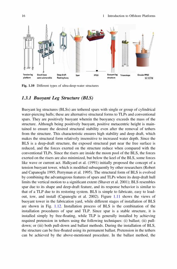
Buoyant leg structures (BLSs) are tethered spars with single or group of cylindricalwater-piercing hulls; these are alternative structural forms to TLPs and conventionalspars. They are positively buoyant wherein the buoyancy exceeds the mass of thestructure. Although being positively buoyant, positive metacentric height is main-tained to ensure the desired structural stability even after the removal of tethersfrom the structure. This characteristic ensures high stability and deep draft, whichmakes the structural form relatively insensitive to increased water depth. Since theBLS is a deep-draft structure, the exposed structural part near the free surface isreduced, and the forces exerted on the structure reduce when compared with theconventional TLPs. Since the risers are inside the moon pool of the BLS, the forcesexerted on the risers are also minimized, but below the keel of the BLS, some forceslike wave or current act. Halkyard et al. (1991) initially proposed the concept of atension buoyant tower, which is modified subsequently by other researchers (Robertand Capanoglu 1995; Perryman et al. 1995). The structural form of BLS is evolvedby combining the advantageous features of spars and TLPs where its deep-draft hulllimits the vertical motion to a significant extent (Shaver et al. 2001); BLS resemblesspar due to its shape and deep-draft feature, and its response behavior is similar tothat of a TLP due to its restoring system. BLS is simple to fabricate, easy to load-out, tow, and install (Capanoglu et al. 2002). Figure 1.11 shows the views ofbuoyant tower in the fabrication yard, while different stages of installation of BLSare shown in Fig. 1.12. Installation process of BLS is the combination of theinstallation procedures of spar and TLP. Since spar is a stable structure, it isinstalled simply by free-floating, while TLP is generally installed by achievingrequired pretension in tethers using the following techniques: (i) ballast; (ii) pull-down; or (iii) both pull-down and ballast methods. During the installation of BLS,the structure can be free-floated using its permanent ballast. Pretension in the tetherscan be achieved by the above-mentioned procedure. In the ballast method, the
Fig. 1.10 Different types of ultra-deep-water structures
16 1 Introduction to Offshore Platforms
structure is additionally ballasted until it achieves the required draft; tethers are thenattached from the structure to the seafloor. Additional ballast is removed from thestructure to enable pretension in the tethers. In the pull-down method, free-floatingstructure is pulled down until it achieves the required draft; excess buoyancy that istransferred to the tethers helps to achieve the desired pretension. Pull-down andballast methods are the combination of the above-mentioned procedures. BLSimposes improved motion characteristics and more convenient riser systems, asthey consist of simple hulls in comparison with spars or TLPs. BLS is moreeconomic than TLPs or spars due to the reduced cost of commissioning. The firstbuoyant tower drilling production platform, CX-15 for Peru’s Corvina offshorefield, is installed in September 2012 at a water depth of more than 250 m with aproduction capacity of 12,200 barrels per day.
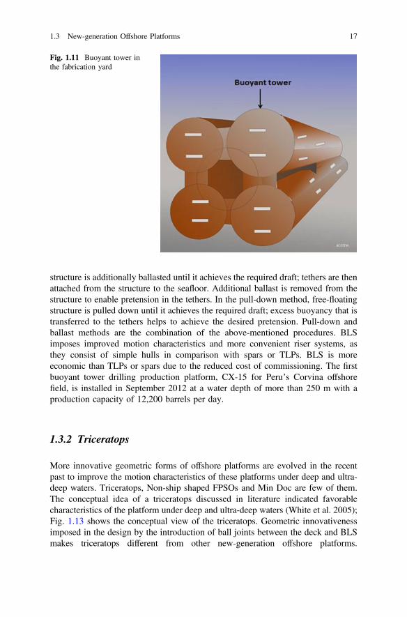
1.3.2 Triceratops
More innovative geometric forms of offshore platforms are evolved in the recentpast to improve the motion characteristics of these platforms under deep and ultra-deep waters. Triceratops, Non-ship shaped FPSOs and Min Doc are few of them.The conceptual idea of a triceratops discussed in literature indicated favorablecharacteristics of the platform under deep and ultra-deep waters (White et al. 2005);Fig. 1.13 shows the conceptual view of the triceratops. Geometric innovativenessimposed in the design by the introduction of ball joints between the deck and BLSmakes triceratops different from other new-generation offshore platforms.
Fig. 1.11 Buoyant tower inthe fabrication yard
1.3 New-generation Offshore Platforms 17
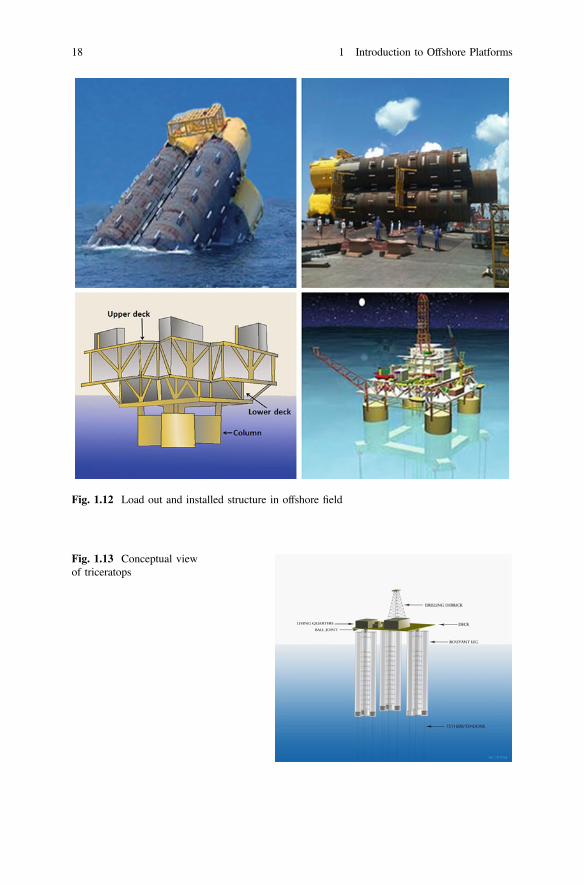
Fig. 1.12 Load out and installed structure in offshore field
Fig. 1.13 Conceptual viewof triceratops
18 1 Introduction to Offshore Platforms
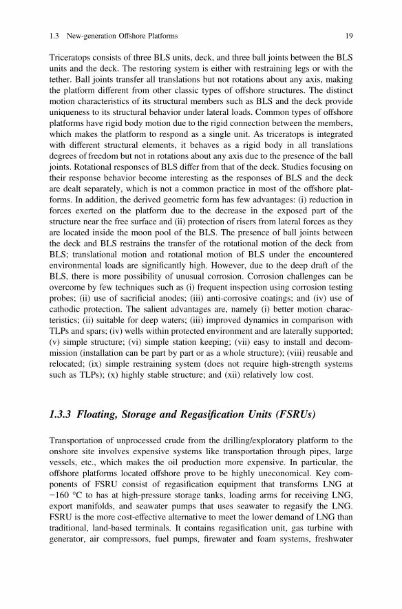
Triceratops consists of three BLS units, deck, and three ball joints between the BLSunits and the deck. The restoring system is either with restraining legs or with thetether. Ball joints transfer all translations but not rotations about any axis, makingthe platform different from other classic types of offshore structures. The distinctmotion characteristics of its structural members such as BLS and the deck provideuniqueness to its structural behavior under lateral loads. Common types of offshoreplatforms have rigid body motion due to the rigid connection between the members,which makes the platform to respond as a single unit. As triceratops is integratedwith different structural elements, it behaves as a rigid body in all translationsdegrees of freedom but not in rotations about any axis due to the presence of the balljoints. Rotational responses of BLS differ from that of the deck. Studies focusing ontheir response behavior become interesting as the responses of BLS and the deckare dealt separately, which is not a common practice in most of the offshore plat-forms. In addition, the derived geometric form has few advantages: (i) reduction inforces exerted on the platform due to the decrease in the exposed part of thestructure near the free surface and (ii) protection of risers from lateral forces as theyare located inside the moon pool of the BLS. The presence of ball joints betweenthe deck and BLS restrains the transfer of the rotational motion of the deck fromBLS; translational motion and rotational motion of BLS under the encounteredenvironmental loads are significantly high. However, due to the deep draft of theBLS, there is more possibility of unusual corrosion. Corrosion challenges can beovercome by few techniques such as (i) frequent inspection using corrosion testingprobes; (ii) use of sacrificial anodes; (iii) anti-corrosive coatings; and (iv) use ofcathodic protection. The salient advantages are, namely (i) better motion charac-teristics; (ii) suitable for deep waters; (iii) improved dynamics in comparison withTLPs and spars; (iv) wells within protected environment and are laterally supported;(v) simple structure; (vi) simple station keeping; (vii) easy to install and decom-mission (installation can be part by part or as a whole structure); (viii) reusable andrelocated; (ix) simple restraining system (does not require high-strength systemssuch as TLPs); (x) highly stable structure; and (xii) relatively low cost.
1.3.3 Floating, Storage and Regasification Units (FSRUs)
Transportation of unprocessed crude from the drilling/exploratory platform to theonshore site involves expensive systems like transportation through pipes, largevessels, etc., which makes the oil production more expensive. In particular, theoffshore platforms located offshore prove to be highly uneconomical. Key com-ponents of FSRU consist of regasification equipment that transforms LNG at−160 °C to has at high-pressure storage tanks, loading arms for receiving LNG,export manifolds, and seawater pumps that uses seawater to regasify the LNG.FSRU is the more cost-effective alternative to meet the lower demand of LNG thantraditional, land-based terminals. It contains regasification unit, gas turbine withgenerator, air compressors, fuel pumps, firewater and foam systems, freshwater
1.3 New-generation Offshore Platforms 19
systems, cranes, lubrication oil system, lifeboats, and helipad. The LNG is stored at−160° in double-walled insulated tanks to limit boil-off. The outer walls of the tankare made of prestressed reinforced concrete or steel to limit the temperature duringstorage period. Despite the high-quality insulation, a small amount of heat stillpenetrates the LNG tanks, causing minor evaporation. The resulting boil-off gas iscaptured and fed back into the LNG tank using compressor and recondensingsystems. This recycling process prevents any natural gas from escaping the terminalunder normal operating conditions. The LNG is subsequently extracted from thetanks, pressurized, and regasified using heat exchangers. The tanks are equippedwith submerged pumps that transfer the LNG toward other high-pressure pumps.The compressed LNG (at around 80 times atmospheric pressure) is then turned backinto a gaseous state in vaporizers. Once returned to its gaseous state, the natural gasis treated in a number of ways, including metering and odorizing, before it is fedinto the transmission network.
The LNG is warmed using the heat from the seawater. This is done in a heatexchanger (with no contact between the gas and the seawater), resulting in a slightdrop in the temperature of the seawater, which reaches 6 °C at the end of thedischarge pipe, quickly becoming imperceptible once diluted. Natural gas isodorless. Although non-toxic, it is inflammable and is odorized to ensure even theslightest leak can be identified. This is done by injecting tetrahydrothiophene(THT), which is an odorant detectable in very small doses, at the terminal before thenatural gas is distributed.
Gas turbine equipped at the topside of the FSRU uses multiple units of gener-ating capacity of up to 10–12 MW. The instrument air system provides air for theplant and the instrument air in process control and maintenance. Inert gas (nitrogen)is generated on demand by a membrane package using dry, compressed air. Abackup inert gas supply system consisting of compressor seals, cooling medium,expansion drums, and utility stations is also provided. The oil pump provides high-pressure oil to the engine. The fuel is pumped from the fuel tank to the primary fuelfilter/water separator, which is then pressurized to 650 kPa gauge pressure by thefuel transfer pump. The pressurized fuel is passed through the secondary/tertiaryfuel filter. Water supply for the fire-fighting systems is supplied by firewater pumpsat a pumping rate of about 600–5,000 m3/h at the discharge flange at a pressure ofabout 18 bar. A film-forming fluoroprotein (FFFP) concentrate system is providedto enhance the effectiveness of the deluge water spray that protects the separatormodule, which has high potential for hydrocarbon pool fires. FFFP is a naturalprotein foaming agent that is biodegradable and non-toxic. The freshwater makersystem will utilize a reverse osmosis process to desalinate the seawater at the rate of5 m3/h. The saline effluent from the freshwater is directed overboard through theseawater discharge caissons, while the freshwater will be stored in a freshwatertank. Water delivered to the accommodation module is further sterilized in a UVsterilization plant before stored in a potable water header tank. The lubricationsystem contains an oil cooler, oil filter, gear-driven oil pump, pre-lube pump, and anoil pan that meets offshore tilt requirements. The internal lubrication system isdesigned to provide a constant supply of filtered, high-pressure oil. This system
20 1 Introduction to Offshore Platforms

meets the tilt requirements for non-emergency offshore operations. Lubrication oilshould have special features in offshore requirements such as (i) water solubility;(ii) non-sheering on water surface; (iii) excellent lubrication properties; (iv) bio-degradable; and (v) non-toxic to aquatic environment.
Exercise
1. With the depletion of onshore and offshore shallow water reserves,the______________________________________ of oil in deep waters hasbecome a challenge to offshore industry.
2. An offshore structure has no ________________ access to dry land and may berequired to stay in ____________ in all weather conditions.
3. _________________________ differs from the other fixed structures strictly byweight contained in their base structure.
4. Most floating production systems and virtually all semisubmersibles, FPSs andFPSOs, produce oil and gas from the wells on the seabed called__________________________.
5. _____________________ generally show very high displacements, whichdemands protection of the well casings from the environment.
6. The tension leg platform is heave restrained by _________________.7. Deep-water floating production systems are generally concentrated in
________________.8. Offshore structures are classified by two independent parameters, namely
__________ and _____________.9. A mobile offshore drilling unit [MODU] configuration is largely determined by
two parameters, namely________________ and ________________.10. Production units have several functions such as ________, _________,
_________, _________, _________, and __________.11. Functional requirements for offshore facilities are determined by the primary
variables _________, __________, and ______________.12. Functional operation of offshore structures influences the _______________ of
the structure.13. List two desirable characteristics of exploratory drilling platforms deployed in
extreme sea states: _____________ and ____________.14. Three of the most common forms of drilling platforms are ____________,
_______________, and __________.15. Drilling platforms with _______________ and _____________ are set on the
seafloor by ___________________.16. Semisubmersibles have good ______________________ in severe environ-
ments and stay longer in drilling modes.17. Jack-up rigs are usually _______________ during transit and are _________
from one site to the other.
1.3 New-generation Offshore Platforms 21

18. In shallow waters, the most common type of production platform is____________________.
19. Production techniques may originate from _________________, and drillingmay be performed with _____________________.
20. Storage capacity of the structure is governed by the ____________ and_______________.
21. Bottom-founded structure with notable exception in terms of constructionmaterial is ________________.
22. Bottom-supported structures are also called as ____________.23. Fixed structure behaves as a _________________ and usually resists the lateral
loads encountered.24. __________________ bottom-supported structures are usually designed such
that their lowest natural frequency is below the energy content of the__________.
25. ______, ___________, and ____________ cause the offshore structures todeflect.
26. ____________ is achieved through taut moorings anchored to the seabed.27. Floating structures have various __________________________.28. __________ such as semisubmersible, spars, and drill ships are _____________
unrestrained and are allowed to have ___________ degrees of freedom such as______________________________________________________.
29. ________________ such as tension leg platform, tethered buoyant towers, orbuoyant leg structures are ______________ to the seabed and _________restrained.
30. Match the following:
1. Payload of bottom-supported structure (a) Resisted by vessel inertia and stability,mooring strength
2. Regulatory and design practices: floatingstructure
(b) Buoyancy
3. Environmental loads of floating structure (c) Resisted by foundation bearing capacity
4. Construction of bottom-supportedstructure
(d) Resisted by strength of the structureand foundation, compliant structure inertia
5. Payload of floating structure (e) Tubular space frame: fabrication yards
6. Installation of bottom-supported structure (f) Plate and frame displacement hull :ship yards
7. Regulatory and design practices: bottom-supported
(g) Barge (dry) transport and launch, upend,piled foundation
8. Construction of floating structure (h) Wet or dry transport, towing to siteand attachment to preinstalled moorings
9. Installation of floating structure (i) Oil industry practices and governmentpetroleum regulation
10. Environmental loads ofbottom-supported structure
(j) Oil industry practices, governmentpetroleum regulation, and coast guard andinternational maritime regulations
22 1 Introduction to Offshore Platforms

31. _______________ platform is typically controlled by their functional gravityloads and lateral force and overturning moments due to wind, wave, andcurrent.
32. For floating structure, it is necessary to evaluate __________ loads due to_____________.
33. ___________ is a term used to define a system for keeping the facility within aspecified distance at the desired location.
34. Jack-up rigs are primarily used for __________; similar to __________ withmovable legs.
35. Semisubmersibles are __________ type of offshore structures, which are pri-marily designed for _________ and ____________purposes.
36. Drill ships are primarily used for ______________.37. Tension leg platform is primarily designed for _______________, which is
developed from semisubmersibles that are _____________ to the seafloor withtethers.
38. __________ is designed primarily for production with a composition of steelframed tubular structure attached to seabed with piles driven into seafloors.
39. _______ are typically large reinforced concrete, bottom-mounted structurewhich resist the lateral loads by its self-weight.
40. ________________ is a structure designed for small field production, which iscomposed of slender truss steel structure supported by __________ foundation.
Answers
1. Exploration and production2. Fixed access; position3. Gravity-based structure4. Subsea wells5. Floating platforms6. Vertical tendons or tethers7. Gulf of Mexico8. Functions and configurations9. Variable deck payload and transit speed requirements
10. Processing, drilling, work over, accommodation, oil storage, and riser support11. Reservoir and fluid characteristics, water depth, and ocean environment12. Configuration13. Limited structural motions and good station keeping14. Drill ships, jack-up barges, and semisubmersibles15. Buoyant legs and pontoons; ballasting16. Motion characteristics17. Buoyant; towed18. Fixed piled structures or jacket structures
Exercise 23

19. Wet or dry tress; subsea blowout preventer (BOP) or surface BOP.20. Size of the shuttle tankers and frequency of the ships21. Gravity-based structure22. Fixed structure23. Rigid body24. Compliant; waves25. Waves, wind, and current26. Compliancy27. Degrees of compliancy28. Neutrally buoyant structures; dynamically; six; heave surge, sway, pitch, roll,
and yaw29. Positively buoyant structures; tethered; heave30. 1(c); 2(j); 3(a); 4(e); 5(b); 6(g); 7(i); 8(f); 9(h); 10(d)31. Fixed32. Inertial; acceleration33. Station keeping34. Exploratory drilling; barge35. Floating; exploratory and production36. Exploratory drilling37. Production; tethered38. Fixed jacketed structure39. Gravity-based structures40. Guyed tower; spud can
24 1 Introduction to Offshore Platforms
Chapter 2Environmental Forces
Abstract This chapter deals with different types of environmental loads on offshorestructures. It also includes code information regarding the loads. Step-by-stepmethod for load estimate on a cylindrical member and an example structure isdetailed. The procedure for estimating wave loads is illustrated through examples.Solved numerical examples and exercise are given at the end for practice.
Keywords Wind forces � Wave forces � Aerodynamic admittance function �Current forces �Wave theories �Marine growth � Design requirements � Allowablestress method � Limit state method � Fabrication and erection loads
2.1 Introduction
Loads acting on offshore structures are classified into the following categories:
• Permanent loads or dead loads• Operating loads or live loads• Other environmental loads including earthquake loads• Construction and installation loads• Accidental loads
While the design of buildings onshore is influenced mainly by the permanentand operating loads, the design of offshore structures is dominated by environ-mental loads, especially waves, and the loads arising in the various stages ofconstruction and installation. In civil engineering, earthquakes are normallyregarded as accidental loads (see Eurocode 8), but in offshore engineering, they aretreated as environmental loads.
Environmental loads are those caused by environmental phenomena. Theseinclude wind, waves, current, tides, earthquakes, temperature, ice, seabed move-ment, and marine growth. Their characteristic parameters, defining design loadvalues, are determined in special studies on the basis of available data. According to
© Springer India 2015S. Chandrasekaran, Dynamic Analysis and Design of Offshore Structures,Ocean Engineering & Oceanography 5, DOI 10.1007/978-81-322-2277-4_2
25
US and Norwegian regulations (or codes of practice), the mean recurrence intervalfor the corresponding design event must be 100 years, while according to theBritish rules, it should be 50 years or greater. The different loads to be consideredwhile designing the structure are wind loads, wave load, mass, damping, ice load,seismic load, current load, dead load, live load, impact load, etc.
2.2 Wind Force
Wind forces on offshore structures are caused by complex fluid-dynamics phe-nomenon, which is generally difficult to calculate with high accuracy. Most widelyused engineering approaches to estimate wind forces on offshore structures arebased on few observations as listed below:
• When stream of air flows with constant velocity (v), it will generate force on theflat plate of area (A).
• The plate will be placed orthogonal to the flow direction.• This force will be proportional to (Av2).• The proportionality constant is independent of the area, which is verified by
experimental studies.
Hence, the wind force on a plate orthogonal to the wind flow direction can bedetermined by the net wind pressure as given below:
pw ¼ 12qaCwv
2 ð2:1Þ
where qa is mass density of air (1.25 kg/m3), and Cw is wind pressure coefficient. Itis important to note that the mass density of air increases due to the water spray(splash) up to a height of 20–20 m above MSL. Hence, the total wind-induced forceon the plate is given by:
Fw ¼ pwA ð2:2Þ
If the plate has an angle ðhÞ with respect to the wind direction, then theappropriate projected area, normal to the flow direction, should be used in the aboveequation. The wind pressure coefficient Cw is determined under controlled sta-tionary wind flow conditions in a wind tunnel. It depends on the Reynolds number;typical values of 0.7–1.2 are used for cylindrical members. Natural wind has twocomponents: (i) mean wind component (which is static component) and (ii) fluc-tuating, gust component (which is a dynamic component). The gust component isgenerated by the turbulence of the flow field in all the three spatial directions. Foroffshore locations, mean wind speed is much greater than the gust component,which means that in most of the design cases, a static analysis will suffice. The windvelocity is given by:
26 2 Environmental Forces
vðtÞ ¼ �vþ vðtÞ ð2:3Þ
where �vffiffiffiffiffiffiffiffiffiffiffiffiffiffiffia2 þ b2
pis the mean wind velocity and v(t) is the gust component. The
spatial dependence of the mean component is only through the vertical coordinate,while v(t) is homogeneous in both space and time. Wind force in the directionsparallel (drag force) and normal to the wind direction (lift force) is given by:
FD ¼ 12qCD�vzA
FL ¼ 12qCL�vzA
ð2:4Þ
Wind spectrum above water surface is given by 1/7th power law, which is:
vz ¼ V10z10
h i 17
ð2:5Þ
where vz is the wind speed at elevation of z m above MSL, V10 is the wind speed at10 m above MSL, and 10 m is called the reference height. Power law is purelyempirical and most widely used. It is tested with the actual field measurements andfound to be in good agreement. As Eq. (2.5) gives mean wind component, the gustcomponent can be obtained by multiplying a gust factor with the sustained windspeed. Average gust factor (Fg) is in the range of 1.35–1.45; variation of the gustfactor along the height is negligible. The sustained wind speed, which is to be usedin the design, is the one minute average wind speed, according to the US WeatherBureau. The product of sustained wind speed and the gust factor will give thefastest mile velocity. 200 year sustained wind velocity of 125 miles per hour is to beused for the design of offshore structures.
Wind produces a low-frequency excitation. The fluctuating component ismodeled probabilistically. Drag force on the members is caused by the encounteredwaves and wind. Wave forces alone acting on the member will cause inertia anddrag forces, while earthquake forces cause only inertia forces on the members.Hence, vibration of the structure induced by wind and waves is different from thatcaused by earthquakes. For the design of members under wind loads, most of theinternational codes prefer quasi-static analysis. Very slender and flexible structuresare wind-prone; for members under wave action, de-amplification takes place inflexible structures due to compliancy. While considering wind as a dynamic pro-cess, the following parameters are important:
• Length of the record: The record can be continuous, intermittent or a selectivewhose values are usually above the threshold ones. For the record to be con-tinuous, average values of the wind velocity is lesser than that of the intermittentbecause of the longer length of the record when compared with the former.
• Wind spectrum: It is used as input for the structural analysis, which defines thefluctuating wind component.
• Gust component: It is approximated by the aerodynamic admittance function.
2.2 Wind Force 27
Aerodynamic admittance function is an intelligent way to define the cross-spectrum in the analysis, indirectly. There are two reasons for using the aerodynamicadmittance function: (i) to bypass the rigorous random analysis and (ii) possibility ofan accurate measurement of this function through wind-tunnel experiments. In thismanner, the spatial variations of wind velocity are handled intelligently in the design.Force due to wind is given by:
FwðtÞ ¼ 12qaCwv
2A
¼ 12qaCwA �vþ vðtÞ½ �2
¼ 12qaCwA �v2 þ vðtÞð Þ2þ2�vvðtÞ
h iby neglecting higher powers of gust component,
ffi �Fw þ qaCwA�vvðtÞ
ð2:6Þ
In the above equation, wind force is expressed as a sum of mean component and thegust component. Wind is considered as an ergodic process; the (one-sided) powerspectral density of the wind process is then related to the wind spectrum as:
SþF ðxÞ ¼ qaCw A �v½ �2SþUðxÞ ð2:7Þ
Substituting Eq. (2.2) in Eq. (2.7) and rearranging the terms, we get:
SþF ðxÞ ¼4 �Fw½ �2½�v�2 v
xffiffiffiA
p
2p�v
� �� �2SþUðxÞ ð2:8Þ
In the above equation, force and the response spectra are connected by the aero-dynamic admittance function, which varies as below:
forx
ffiffiffiA
p
2p�v) 0; v
xffiffiffiA
p
2p�v
� �) 1
forx
ffiffiffiA
p
2p�v) 1; v
xffiffiffiA
p
2p�v
� �) 0
ð2:9Þ
Aerodynamic admittance function is proposed through an empirical relationship byDavenport (1977):
vðxÞ ¼ 1
1þ ð2xÞ4=3h i
8<:
9=; ð2:10Þ
28 2 Environmental Forces
Wind spectra for the design of offshore structures are listed below with thedetails. For the reference height of z = 10 m, wind spectra as applied to offshorestructures are expressed in terms of circular frequency as given below:
Sþu xð Þ ¼ fGþu fð Þ ð2:11Þ
(i) Davenport spectrum
xSþu xð ÞdU
2p
¼ 4h2
1þ h2� �4=3 ð2:12Þ
(ii) Harris spectrum
xSþu xð ÞdU
2p
¼ 4h
2þ h2� �5=6 ð2:13Þ
Derivable variable h is given by:
h ¼ xLu2pU10
¼ dLuU10
; 0\h\1 ð2:14Þ
where Lu is integral length scale (=1,200 m for Davenport and 1,800 m for Harrisspectrum), d is surface drag coefficient referred to �U10. For offshore locations,d ¼ 0:001. It is important to note that none of these spectrum used in the analysis ofwind speed is recorded offshore; they are based on onshore records. Hence, theseapplications to offshore locations are questionable. They have serious problemwhen used for low-frequency flexible structures. Alternatively, for large floatingstructures, following spectra are recommended by Dyrbye and Hassen (1997):
(a) Kaimal spectrum
xSþu xð Þr2u
¼ 6:8 h
1þ 10:2 hð Þ5=3ð2:15Þ
where r2u is the variance of U(t) at reference height of 10 m?(b) API (2000) spectrum
xSþu xð Þru zð Þ2 ¼
xxp
�1þ 1:5 x
xp
�h i5=3 ð2:16Þ
2.2 Wind Force 29
where xp is peak frequency and r2z is the variance of U(t), which is notassumed as independent.
0:01� xpz
U zð Þ � 0:1 ð2:17Þ
Usually, a value of 0.025 is obtained in lieu of the values computed from theabove equation. Standard deviation and speed are given by:
ru zð Þ ¼ 0:15U zð Þ ZsZ
� �0:125:Z� Zs
0:15U zð Þ ZsZ
� �0:275:Z[ Zs
(ð2:18Þ
where Zs is the thickness of the surface layer, which is usually taken as 20 m.
2.3 Wave Forces
Wind-generated sea surface waves shall be represented as a combination of series ofregular waves. Regular waves of different magnitude and wave lengths from dif-ferent directions are combined to represent the sea surface elevation. Water particlekinematics of regular waves is expressed by the sea surface elevation by variouswave theories (Srinivasan and Bhattacharyya 2012). Among all the theories, Airy’swave theory is commonly used because it assumes linearity between the kinematicquantities and the wave height, which makes the wave theory simple. Airy’s theoryassumes a sinusoidal wave form of wave height (H), which is small in comparisonwith the wave length (k) and water depth (d) as given below:
gðx; tÞ ¼ H2cosðkx� xtÞ
k ¼ 2pk
_uðx; tÞ ¼ xH2
coshðkyÞsinhðkdÞ cosðkx� xtÞ
_vðx; tÞ ¼ xH2
sinhðkyÞsinhðkdÞ sinðkx� xtÞ
€uðx; tÞ ¼ x2H2
coshðkyÞsinhðkdÞ sinðkx� xtÞ
€vðx; tÞ ¼ �x2H2
sinhðkyÞsinhðkdÞ cosðkx� xtÞ
ð2:19Þ
30 2 Environmental Forces
Airy’s theory is valid up to mean sea level only. However, due to the variablesubmergence effect, the submerged length of the members will be continuouslychanging. This will attract additional forces due to their variable submergence atany given time. To compute the water particle kinematics up to the actual level ofsubmergence, stretching modifications suggested by various researchers are used.
(a) Wheeler suggested the following modification in the horizontal water particlevelocity and acceleration to include the actual level of submergence of themember:
_uðx; tÞ ¼ xH2
cosh ky ddþg
h i �sinhðkdÞ cosðkx� xtÞ
€uðx; tÞ ¼ x2H2
cosh ky ddþg
h i �sinhðkdÞ sinðkx� xtÞ
ð2:20Þ
(b) Chakrabarti suggested the modification as given below:
_uðx; tÞ ¼ xH2
cosh kyð Þsinhðkðd þ gÞÞ cosðkx� xtÞ
€uðx; tÞ ¼ x2H2
cosh kyð Þsinhðkðd þ gÞÞ sinðkx� xtÞ
ð2:21Þ
The sea state, in a short term, which is typically 3 h, is assumed as zero-mean,ergodic Gaussian process. This can be defined completely by a wave spectrum. ForNorth Sea, Johnswap spectrum is recommended. For open sea conditions, Peirson–Moskowitz (P–M) spectrum is recommended. In a long term, variation of sea stateis slower than the short-term fluctuations. It is often approximated by a series ofstationary, non-zero-mean Gaussian process, which is specified by the significantwave height (Hs) and peak wave period (Tp). Following are a few relevant spectra,applicable in the design of offshore platforms.
2.4 Wave Theories
Wave theories serve to calculate the particle velocities, accelerations, and thedynamic pressure as functions of the surface elevation of the waves. For long-crested regular waves, the flow can be considered two-dimensional and are char-acterized by parameters such as wave height (H), period (T) and water depth (d), asshown in Fig. 2.1. k ¼ 2p=L denotes the wave number, x ¼ 2p=T denotes thewave circular frequency, and f ¼ 1=T denotes the cyclic frequency. Different wavetheories available are as follows:
2.3 Wave Forces 31
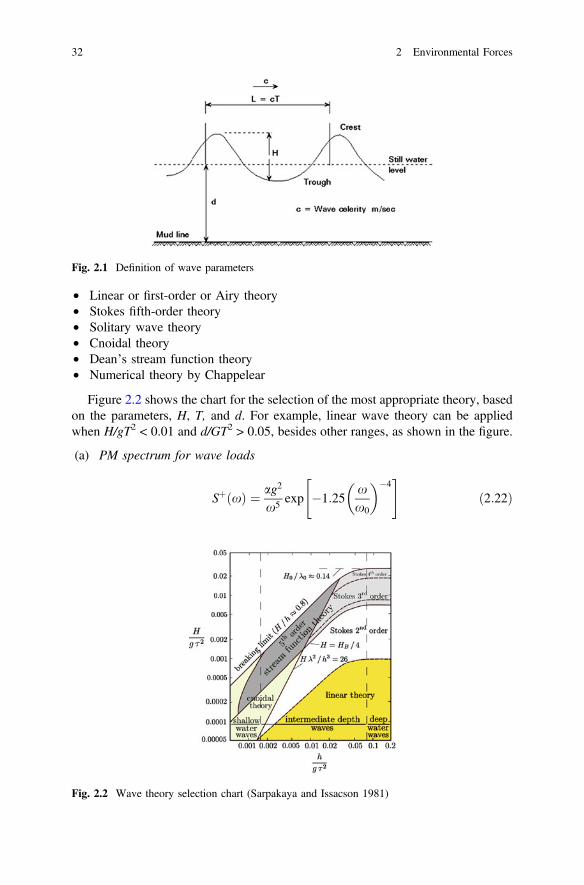
• Linear or first-order or Airy theory• Stokes fifth-order theory• Solitary wave theory• Cnoidal theory• Dean’s stream function theory• Numerical theory by Chappelear
Figure 2.2 shows the chart for the selection of the most appropriate theory, basedon the parameters, H, T, and d. For example, linear wave theory can be appliedwhen H/gT2 < 0.01 and d/GT2 > 0.05, besides other ranges, as shown in the figure.
(a) PM spectrum for wave loads
Sþ xð Þ ¼ ag2
x5 exp �1:25xx0
� �4" #
ð2:22Þ
Fig. 2.1 Definition of wave parameters
Fig. 2.2 Wave theory selection chart (Sarpakaya and Issacson 1981)
32 2 Environmental Forces
where a is Phillips constant ffi 0.0081.(b) Modified PM spectrum (2 parameters Hs;x0)
Sþ xð Þ ¼ 516
Hsx4
0
x5 exp �1:25xx0
� �4" #
ð2:23Þ
(c) International Ship Structures Congress (ISSC) spectrum (2 parameters Hs, �x)
Sþ xð Þ ¼ 0:1107Hsx�4
x5 exp �0:4427x�x
��4� �
x ¼ M1
M0
ð2:24Þ
where M1 and M0 are spectral moments.(d) Johnswap spectrum (5 parameters Hs;x0o; c; sa; sbÞ
Sþ xð Þ ¼ ag2
x5 exp �1:25xx0
� �4" #
caðxÞ ð2:25Þ
where c is the peakness parameter.
a xð Þ ¼ exp � x� x0ð Þ22r2x2
0
" #ð2:26Þ
where �r is spectral width parameter and is given by:
ra ¼ 0:07; x�x0 ð2:27Þ
rb ¼ 0:09; x[x0 ð2:28Þ
The modified Phillips constant is given by:
a ¼ 3:25� 10�3H2sx
40 1� 0:287 ln cð Þ½ � ð2:29Þ
c ¼ 5 forTpffiffiffiffiffiHs
p � 3:6 ð2:30Þ
¼ exp 5:75� 1:15TpffiffiffiffiffiHs
p� �
forTpffiffiffiffiffiHs
p [ 3:6 ð2:31Þ
Hs ¼ 4ffiffiffiffiffiffim0
p ð2:32Þ
where c varies from 1 to 7.
2.4 Wave Theories 33
Main force components, rising from the wave loads, are grouped as follows:(i) Froude–Krylov force, which is caused by the pressure effects due to the undisturbedincident waves; (ii) diffraction force, which is caused by the pressure effects due tothe presence of the structure in the fluid-flow domain; (iii) hydrodynamic addedmass and potential damping forces, which is caused by the pressure effects due tothe motion of the structural components in ideal fluid; and (iv) viscous drag force,which is caused by the pressure effects due to the relative velocity between thewater particle and the structural component. For slender structures, Froude–Krylovforce and diffraction forces are idealized by a single inertia term. Velocity andacceleration do not differ significantly from the values of the cylinder axis whenD=k < 0.2. When the waves act on the slender structures, the structure oscillates,which will set up waves radiating away from it. Reaction forces are then set up in thefluid, which will be proportional to the acceleration and velocity of the structure.Reaction force proportional to the acceleration of the structure will result in an addedmass term, contributing to the inertia force. Reaction force proportional to thevelocity results in the potential damping force. If the structure is compliant, the addedmass forces associated with the relative acceleration between the fluid particles andthe structures are included. Drag force is computed by replacing the water particlevelocity with the relative velocity term. The total force acting normal to the axis of themember is given by:
qn ¼ q dV � an þ ðCm � 1Þq dVðan � x::nÞ þ 1
2qCd dAðvn � _xnÞ vn � _xnj j
¼ CmqdV � an � ðCm � 1ÞqdV x::n þ 1
2qCd dAðvn � _xnÞ vn � _xnj j
ð2:33Þ
where q is density of fluid, (Cd, Cm) are the drag and inertia coefficients, (vn, an) arevelocity and acceleration of the water particle normal to the axis of the member, _x;€xare the velocity and acceleration of the structure, and (dA, dV) are exposed area anddisplaced volume of water per unit length, respectively.
The above equation has two main issues: first, the relative motion formulation isvalid only if the structure motion is of large amplitude; second, the relative velocityformation of the drag produces both excitation and damping forces. In the aboveequation, the most critical aspect is the evaluation of the drag and inertia coeffi-cients, which is dependent on flow conditions, Keulegan–Carpenter number, andReynolds number. The recommended value of drag coefficient is 0.6–1.2, while thatof the inertia coefficient is 1.2–2.0, as seen in the literature (APR RP 2A). As in thecase of bottom-supported structures (gravity platforms), when the diameter of themember is very large, incident waves are disturbed by the presence of the structure.In such cases, viscous force becomes less significant due to the smaller values of theratio of wave height to member diameter (H/D ≪ 1). In such cases, the aboveequations cannot be applied; it is recommended that the analyzer should usenumerical methods to determine the forces on the members.
Offshore structures have large plane area. Larger topside is required foraccommodating the equipment layout as discussed in the previous chapter. As the
34 2 Environmental Forces
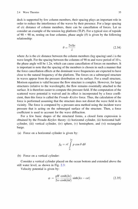
deck is supported by few column members, their spacing plays an important role inorder to reduce the interference of the waves by their presence. For a large spacingof c/c distance of column members, there can be cancellation of forces. Let usconsider an example of the tension leg platform (TLP). For a typical size of topsideof 90 × 90 m, resting on four columns, phase angle (h) is given by the followingrelationship:
h ¼ 2pDxk
ð2:34Þ
where Dx is the c/c distance between the column members (leg spacing) and λ is thewave length. For the spacing between the columns of 90 m and wave period of 10 s,the phase angle will be 1.2π, which can cause cancellation of forces on members. Itis important to note that the spacing of the members is chosen in such a manner thatthe force cancellation effects at the dominant wave frequencies are expected to haveclose to the natural frequency of the platform. The forces on a submerged structurein waves appear from the pressure distribution on its surface. For a small structure,Morison equation is valid because the flow structure is complex. However, for largestructures (relative to the wavelength), the flow remains essentially attached to thesurface. It is therefore easier to compute this pressure field. If the computation of thescattered wave potential is waived and its effect is incorporated by a force coeffi-cient, then this force is called the Froude–Krylov force. Thus, the calculation of theforce is performed assuming that the structure does not distort the wave field in itsvicinity. The force is computed by a pressure-area method using the incident wavepressure that is acting on the submerged surface of the structure. Then, a forcecoefficient is used to account for the wave diffraction.
For a few basic shapes of the structural forms, a closed form expression isobtained by the Froude–Krylov theory: (i) horizontal cylinder, (ii) horizontal half-cylinder, (iii) vertical cylinder, (iv) sphere, (v) hemisphere, and (vi) rectangularbarge.
(a) Force on a horizontal cylinder is given by:
fH ¼ r‘Z2p0
p cos h dh
(b) Force on a vertical cylinder:
Consider a vertical cylinder placed on the ocean bottom and extended above thestill water level, as shown in Fig. 2.3:
Velocity potential is given by:
u ¼ gH2x
coshðksÞcoshðkdÞ sinhðkx� xtÞ ð2:35Þ
2.4 Wave Theories 35
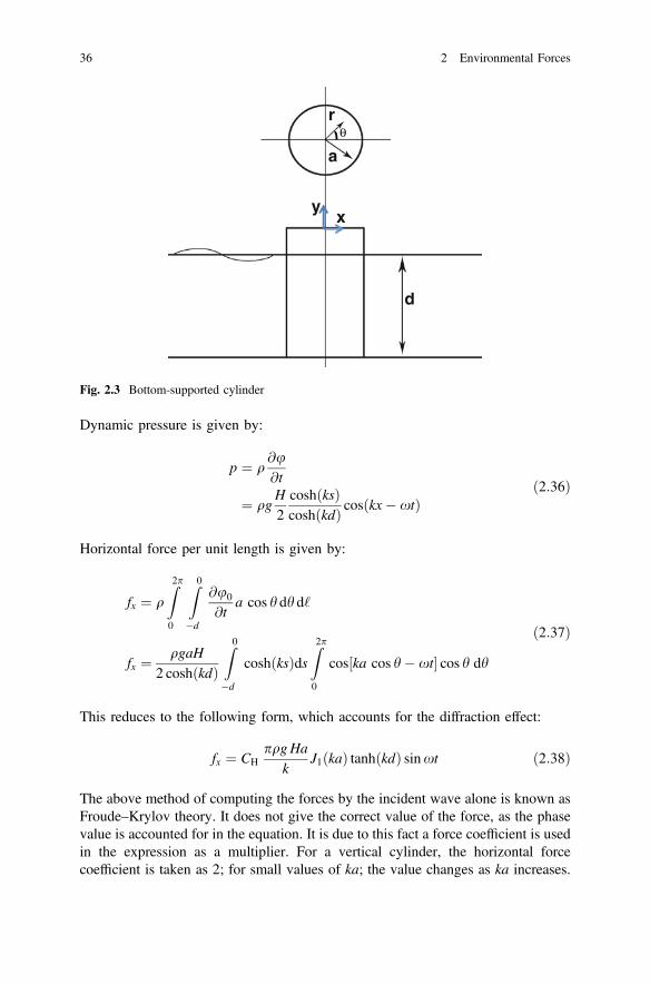
Dynamic pressure is given by:
p ¼ q@u@t
¼ qgH2coshðksÞcoshðkdÞ cosðkx� xtÞ
ð2:36Þ
Horizontal force per unit length is given by:
fx ¼ qZ2p0
Z0
�d
@u0
@ta cos h dh d‘
fx ¼ qgaH2 coshðkdÞ
Z0
�d
coshðksÞdsZ2p0
cos½ka cos h� xt� cos h dh
ð2:37Þ
This reduces to the following form, which accounts for the diffraction effect:
fx ¼ CHpqgHa
kJ1ðkaÞ tanhðkdÞ sinxt ð2:38Þ
The above method of computing the forces by the incident wave alone is known asFroude–Krylov theory. It does not give the correct value of the force, as the phasevalue is accounted for in the equation. It is due to this fact a force coefficient is usedin the expression as a multiplier. For a vertical cylinder, the horizontal forcecoefficient is taken as 2; for small values of ka; the value changes as ka increases.
r
a
d
xy
θ
Fig. 2.3 Bottom-supported cylinder
36 2 Environmental Forces
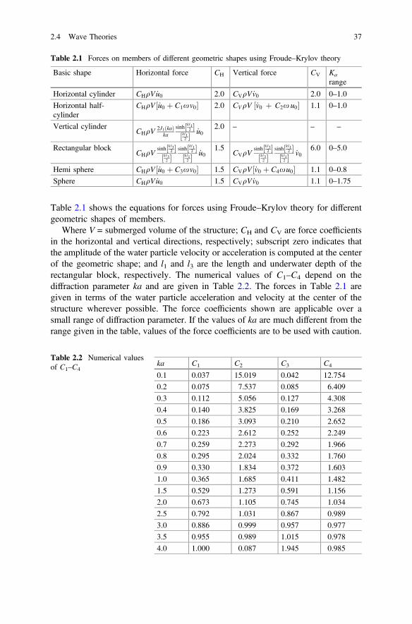
Table 2.1 shows the equations for forces using Froude–Krylov theory for differentgeometric shapes of members.
Where V = submerged volume of the structure; CH and CV are force coefficientsin the horizontal and vertical directions, respectively; subscript zero indicates thatthe amplitude of the water particle velocity or acceleration is computed at the centerof the geometric shape; and l1 and l3 are the length and underwater depth of therectangular block, respectively. The numerical values of C1–C4 depend on thediffraction parameter ka and are given in Table 2.2. The forces in Table 2.1 aregiven in terms of the water particle acceleration and velocity at the center of thestructure wherever possible. The force coefficients shown are applicable over asmall range of diffraction parameter. If the values of ka are much different from therange given in the table, values of the force coefficients are to be used with caution.
Table 2.1 Forces on members of different geometric shapes using Froude–Krylov theory
Basic shape Horizontal force CH Vertical force CV Ka
range
Horizontal cylinder CHqV _u0 2.0 CVqV _v0 2.0 0–1.0
Horizontal half-cylinder
CHqV _u0 þ C1xv0½ � 2.0 CVqV ½_v0 þ C2x u0� 1.1 0–1.0
Vertical cylinderCHqV
2J1ðkaÞka
sinh k‘12½ �
k‘12½ � _u0
2.0 – – –
Rectangular blockCHqV
sinhk‘32½ �
k‘32½ �
sinh k‘12½ �
k‘12½ � _u0
1.5CVqV
sinhk‘32½ �
k‘32½ �
sinh k‘12½ �
k‘12½ � _v0
6.0 0–5.0
Hemi sphere CHqV _u0 þ C3xv0½ � 1.5 CVqV _v0 þ C4xu0½ � 1.1 0–0.8
Sphere CHqV _u0 1.5 CVqV _v0 1.1 0–1.75
Table 2.2 Numerical valuesof C1–C4
ka C1 C2 C3 C4
0.1 0.037 15.019 0.042 12.754
0.2 0.075 7.537 0.085 6.409
0.3 0.112 5.056 0.127 4.308
0.4 0.140 3.825 0.169 3.268
0.5 0.186 3.093 0.210 2.652
0.6 0.223 2.612 0.252 2.249
0.7 0.259 2.273 0.292 1.966
0.8 0.295 2.024 0.332 1.760
0.9 0.330 1.834 0.372 1.603
1.0 0.365 1.685 0.411 1.482
1.5 0.529 1.273 0.591 1.156
2.0 0.673 1.105 0.745 1.034
2.5 0.792 1.031 0.867 0.989
3.0 0.886 0.999 0.957 0.977
3.5 0.955 0.989 1.015 0.978
4.0 1.000 0.087 1.945 0.985
2.4 Wave Theories 37
2.5 Current Forces
The presence of current in water produces the following distinct effects: Currentvelocity should be added vectorially to the horizontal water particle velocity beforecomputing the drag force, because drag force depends on the square of the waterparticle velocity. Current decreases slowly with the increase in depth, but even asmall magnitude of current velocity can cause significant drag force. This effect isinsignificant and generally neglected. Current makes the structure itself to generatewaves, which in turn creates diffraction forces. However, these values are negligiblefor realistic value of current acting on the normal-sized members. The presence ofcurrent is alternatively accounted by increasing the wave height to 10–15 % andneglects the presence of current per se.
2.6 Earthquake Loads
Offshore platforms which do not have stiff connection with the seabed are indirectlyinfluenced by earthquakes; those which are bottom-supported are affected byearthquakes directly. Compliant structures that are position-restrained by tetherswill be subjected to dynamic tether tension variations under the presence ofearthquake forces. This will give rise to the dynamic tether tension variations,which in turn shall affect the response of the platform under lateral loads. Earth-quakes give rise to the horizontal and vertical motions for a typical duration of15–30 s. Earthquake acceleration exhibits random characteristics due to (i) thenature of the mechanism causing earthquakes; (ii) wave propagation; (iii) reflection;and (iv) deflection. Effects of earthquake forces give rise to horizontal and verticalmotions with durations of 15–30 s. Earthquake loads exhibit random characteristicsdue to the nature of the mechanism causing earthquake, wave propagation,reflection, and deflection. Earthquakes can result in inertia forces due to theacceleration and damping forces due to the motion of the water particles.
In case of the analysis of compliant structures like TLPs, earthquake forces arehandled in an indirect manner. Water waves generated due to the ground motion areneglected. Stiffness of TLP tether is modeled as axial tension members; slackeningof tethers is neglected. The dynamic tether tension variation, caused by the hori-zontal motion of the earthquakes, is used to update the stiffness matrix of the TLPusing the following equation (Chandrasekaran and Gaurav 2008):
DT ¼ AE‘
xðtÞ � xgðtÞ� � ð2:39Þ
where x(t) is the instantaneous response vector of TLP and xg(t) is the grounddisplacement vector, which is given by:
38 2 Environmental Forces
xgðtÞ ¼
x1gðtÞ0
x3gðtÞ000
8>>>>>><>>>>>>:
9>>>>>>=>>>>>>;
ð2:40Þ
where x1g and x3g are the horizontal and vertical ground displacements, respec-tively. Ground motions can be generated using Kanai-Tajimi ground accelerationspectrum (K-T spectrum), which is given by:
Sx::gx::gðxÞ ¼ x4
g þ 4n2gx2gx
2
x2g � x2
�2þ 4n2gx2
gx2
264
375S0
S0 ¼2ngr2g
pxgð1þ 4n2gÞ
ð2:41Þ
where S0 is the intensity of earthquake, xg is the natural frequency of the ground, ngis the damping of the ground, and r2g is the variance of the ground acceleration.These are the three parameters on which K-T spectrum depends on, which need to bechosen for any analytical studies on TLP under seismic action. The above threeparameters should be estimated from the representative earthquake records byestablished estimation processes (Chandrasekaran et al. 2006). For example, anearthquake occurred in GoM, approximately at 250 miles WSW of Anna Maria,Florida on September 10, 2006 at 14:56:07 (coordinated universal time). The signalwas epicentered 26.34N, 86.57W. Incidentally, MARS TLP was operating in theMississippi Canyon Block, which is also located in GoM. The three parameters S0,xg, and ng are chosen such that the real earthquake is simulated for analysis purposes(Chandrasekaran and Gaurav 2008). Studies showed that the dynamic tether tensionvariations caused by the earthquake forces are in the order of about 65 % more thanthat of the normal values. Even structures with rigid degrees of freedom like heaveare excited, which may result in the loss of functionality of the platform.
2.7 Ice and Snow Loads
Ice loads are dominant in offshore structures in the Arctic regions. Prediction of iceloads is associated with a significant degree of uncertainty, as there are various iceconditions that exist in the service life of an offshore platform. They are level ice,broken ice, ice ridges, and icebergs. Offshore structures show different types of
2.6 Earthquake Loads 39
failure under ice loads, namely creep, cracking, buckling, spalling, and crushing. Iceloads exhibit random variations in both space and time. They are classified into:(i) total or global loads and (ii) local loads or pressure. Global loads affect the overallmotion and stability of the platform, while local loads affect the members at con-nections. In the level ice condition, frequency of interaction between the structureand ice is important; number of interactions per unit time is important to quantify theice loads on offshore platforms. Total ice force can result in a periodic loading andcan cause dynamic amplification in flexible/slender structures. Current codes includeequations for the extreme static ice loads, which depend on the geometric shape ofthe structure. Studies show that ice loads in a conical structure are lesser than that ofthe cylindrical structure (Sanderson 1988). This is because a well-designed coneshape can change the ice-failure mode from crushing to bending. Estimating (pre-dicting) ice forces on offshore platforms has a lot of uncertainties. Ice forces oftencontrol the design of the platform in operational conditions, in particular. The designice loads use varying factors for level ice, first-year ridge ice, and multi-year ridgeice; the factored values are 2, 5, and 7, respectively.
There are four approaches for addressing ice forces on offshore platforms:(a) experimental studies on scaled models; (b) numerical studies; (c) field studies;and (d) data mining. Experimental studies use scaling laws to determine the iceloads and ice–structure interaction. This method claims many advantages due to thecapability of testing many types of structural shapes in large testing facilities.However, such tests are expensive apart from a strong disagreement of the modelice not being accurately scaled as of the sea ice. As the ice failure is dependent onthe geometric shape significantly, ice-failure behavior cannot be accurately studied.This may result in overprediction of ice loads. Numerical modeling uses high-endsoftware to model ice forces for different interaction scenarios, which makes it verycost-effective and instructive. However, limited validation of results with that of theexperiments is reported in the literature. The more practical way to estimate iceloads is from data mining. Previous platforms can be visited to determine the iceloads through field measurements. This will give a real picture of the ice loads. Inthe frequency domain approach, excitation caused by ice loads is modeled assinusoidal pseudo-excitation, and the response is characterized by the transferfunction. Ice force spectrum on a narrow conical structure is given by:
Sþðf Þ ¼ A�F20�T ð�dÞ
f cexp � B
�T ðaÞf b
� �ð2:42Þ
where A (=10) and B (=5.47) are constants; �F0 is the force amplitude on thestructure; �T ¼ Lb=v is the period of ice; Lb is ice-breaking length, which is typically4–10 times of thickness of ice; v is the velocity; and a; b; c; d are constants whosevalues are typically 0.64, 0.64, 3.5, and 2.5, respectively. Force amplitude on thestructure is given by:
40 2 Environmental Forces
�F0 ¼ C rf h2 D
Lc
� 0:34
ð2:43Þ
where C is the constant; rf is bending strength of ice (0.7 MPa); h is the icethickness; D is the diameter of the ice cone, and Lc is the characteristic length of ice,which is given by the following equation:
Lc ¼ Eh3
12gqw
� �0:25ð2:44Þ
where E is Young’s modulus of ice (=0.5 GPa) and qw is density of water.
2.8 Marine Growth
Marine growth or biofouling is the ubiquitous attachments of soft and hard bio-particles on the surface of a submerged structure. It ranges from seaweeds to hardshelled barnacles. Its growth on the surface of the structure increases its diameterand affects its roughness. Its main effect is to increase the wave forces on themembers by increasing not only exposed areas and volumes, but also the dragcoefficient due to higher surface roughness. In addition, it increases the unit mass ofthe member, resulting in higher gravity loads and in lower member frequencies.Depending upon the geographic location, the thickness of marine growth can reach0.3 m or more. It is accounted for in the design through appropriate increases in thediameters and masses of the submerged members.
2.9 Mass
Mass is contributed by the structural mass and hydrodynamic added mass of thestructure. For a slender structure, mass of the displaced volume of the structure willbe significant and should be considered in the analysis. Added mass depends on thesubmerged volume of the platform, which also varies with respect to period ofvibration. This is due to the variation in buoyancy, which in turn changes the tethertension variation that affects the natural frequency of motion. Based on theequipment layout plan and the chosen structural form, one can compute the mass ofthe platform readily. It is also important to establish the fact that a desired pro-portion between center of buoyancy and center of mass is maintained to ensurestability under free-floating conditions. This is important to enable smooth con-struction process in case of floating.
2.7 Ice and Snow Loads 41
2.10 Damping
For steel offshore structures, structural damping is usually considered to vary from0.2 to 0.5 % of that of the critical damping (Adams and Baltrop 1991). For concretestructures, it can be of the order 0.5–1.5 %. Hydrodynamic damping originates fromthe radiation damping and viscous damping effects. Radiation damping is deter-mined using potential theory. It exhibits a strong dependence on frequency andsubmergence effects. Literature shows that the drag damping is lower for structureswith large diameter column members (*0.1 %). Damping ratio for offshorestructures (wet structures), including the effects of added mass, can be expressed asa ratio of that of the dry structures, as given below:
nwet ¼ nwetðm�
dryÞ ðx�dryÞ
ðm�wetÞ ðx�
wetÞð2:45Þ
where m* and x* are generalized mass and frequency, respectively (Naess andMoan 2013). Literature shows that the total damping ratio is about 2 % for the firstthree modes of bottom-supported structures.
2.11 Dead Load
Dead load is the weight of the overall platform in air, which includes piling,superstructure, jacket, stiffeners, piping, conductors, corrosion anodes, deck, rail-ing, grout, and other appurtenances. Dead load excludes the following: weight ofthe drilling equipment placed on the platform including the derrick, draw works,mud pumps, mud tanks, etc.; weight of production or treatment equipment locatedon the platform including separators, compressors, piping manifolds, and storagetanks; weight of drilling supplies that cause variable loads during drilling such asdrilling mud, water, fuel, casing, etc.; weight of treatment supplies employed duringproduction such as fluid in the separator, storage in the tanks; drilling load, which isapproximate combination of derrick load, pipe storage, rotary table load, etc.
2.12 Live Load
Live loads are acting in addition to the equipment loads. They include load causedby impacts of vessels and boats on the platform. Dynamic amplification factor isapplied to such loads to compute the enhanced live loads. Live loads are generallydesignated as factor times of the applied static load. These factors are assigned bythe designer depending on the type of platform. Table 2.3 gives the live load factorsthat are used in the platform design.
42 2 Environmental Forces
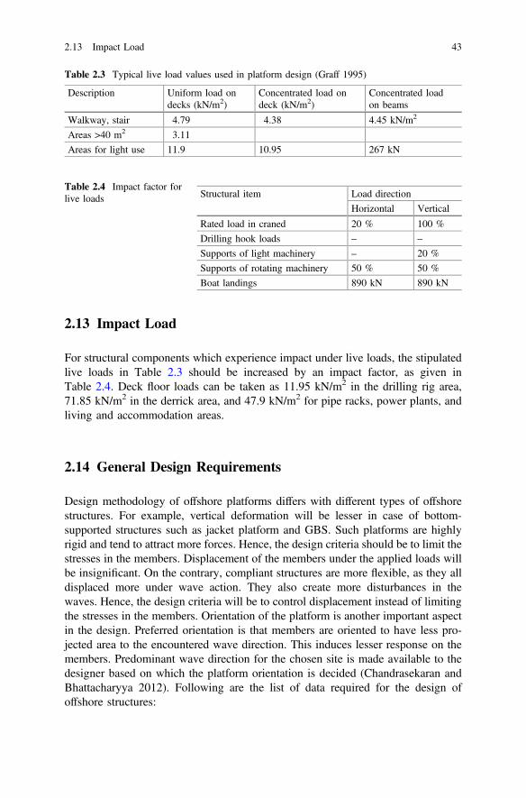
2.13 Impact Load
For structural components which experience impact under live loads, the stipulatedlive loads in Table 2.3 should be increased by an impact factor, as given inTable 2.4. Deck floor loads can be taken as 11.95 kN/m2 in the drilling rig area,71.85 kN/m2 in the derrick area, and 47.9 kN/m2 for pipe racks, power plants, andliving and accommodation areas.
2.14 General Design Requirements
Design methodology of offshore platforms differs with different types of offshorestructures. For example, vertical deformation will be lesser in case of bottom-supported structures such as jacket platform and GBS. Such platforms are highlyrigid and tend to attract more forces. Hence, the design criteria should be to limit thestresses in the members. Displacement of the members under the applied loads willbe insignificant. On the contrary, compliant structures are more flexible, as they alldisplaced more under wave action. They also create more disturbances in thewaves. Hence, the design criteria will be to control displacement instead of limitingthe stresses in the members. Orientation of the platform is another important aspectin the design. Preferred orientation is that members are oriented to have less pro-jected area to the encountered wave direction. This induces lesser response on themembers. Predominant wave direction for the chosen site is made available to thedesigner based on which the platform orientation is decided (Chandrasekaran andBhattacharyya 2012). Following are the list of data required for the design ofoffshore structures:
Table 2.3 Typical live load values used in platform design (Graff 1995)
Description Uniform load ondecks (kN/m2)
Concentrated load ondeck (kN/m2)
Concentrated loadon beams
Walkway, stair 4.79 4.38 4.45 kN/m2
Areas >40 m2 3.11
Areas for light use 11.9 10.95 267 kN
Table 2.4 Impact factor forlive loads Structural item Load direction
Horizontal Vertical
Rated load in craned 20 % 100 %
Drilling hook loads – –
Supports of light machinery – 20 %
Supports of rotating machinery 50 % 50 %
Boat landings 890 kN 890 kN
2.13 Impact Load 43
• Land topographical survey of sufficient area covering the chosen site for plat-form installation
• Hydrographical survey of the proposed location (hydrographic charts are usedfor this purpose)
• Information regarding silting at the site• Wind rose diagram showing information on wind velocities, duration, pre-
dominant direction round the year• Cyclonic tracking data showing details of the past cyclonic storm such as wind
velocities, direction, peak velocity period, etc., are indicated.• Oceanographic data including general tide data, tide table, wave data, local
current, seabed characteristics, temperature, rainfall, and humidity• Seismicity level and values of acceleration• Structural data of existing similar structures, preferably in the close vicinity• Soil investigation report
2.15 Steel Structures
The analysis of an offshore structure is an extensive task, embracing considerationof the different stages, i.e., execution, installation, and in-service stages, during itslife. Many disciplines such as structural, geotechnical, naval architecture, andmetallurgy are involved. The analytical models used in offshore engineering are insome respects similar to those adopted for other types of steel structures. Only thesalient features of offshore models are presented here. The same model is usedthroughout the analysis with only minor adjustments to suit the specific conditions,e.g., at supports in particular, relating to each analysis. Stick models (beam ele-ments assembled in frames) are used extensively for tubular structures (jackets,bridges, and flare booms) and lattice trusses (modules and decks). Each member is(normally) rigidly fixed at its ends to other elements in the model. If more accuracyis required, particularly for the assessment of natural vibration modes, local flexi-bility of the connections may be represented by a joint stiffness matrix. In additionto its geometrical and material properties, each member is characterized byhydrodynamic coefficients, e.g., relating to drag, inertia, and marine growth, toallow wave forces to be automatically generated. Integrated decks and hulls offloating platforms, involving large bulkheads, are described by plate elements. Thecharacteristics assumed for the plate elements depend on the principal state of stressto which they are subjected. Membrane stresses are taken when the element issubjected merely to axial load and shear. Plate stresses are adopted when bendingand lateral pressure is to be taken into account. After developing a preliminarymodel for analysis, member stresses are checked for preliminary sizing under dif-ferent environmental loads.
The verification of an element consists of comparing its characteristic resistance(s)to a design force or stress. It includes (i) a strength check where the characteristicresistance is related to the yield strength of the element and (ii) a stability check for
44 2 Environmental Forces
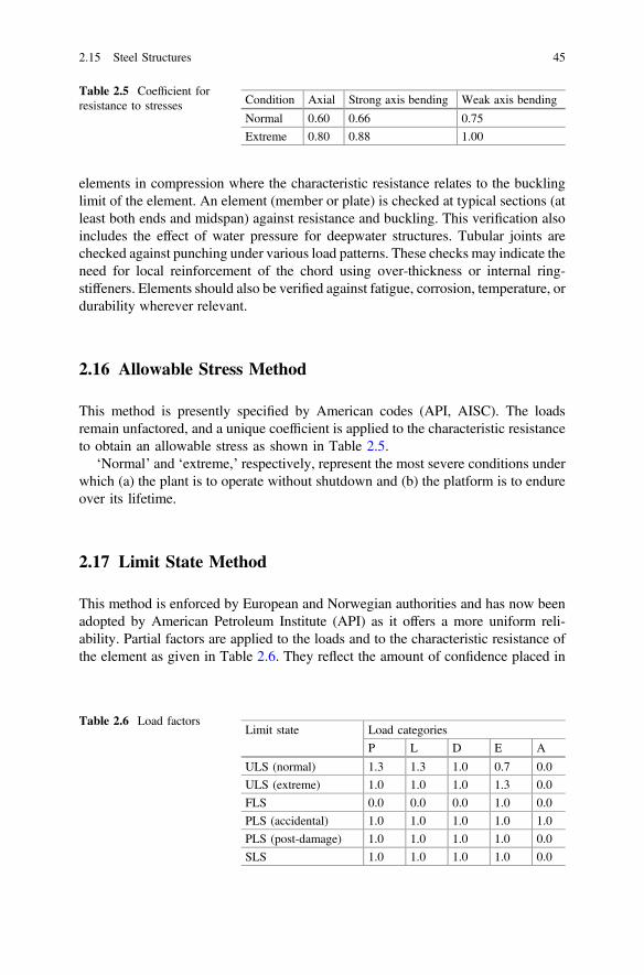
elements in compression where the characteristic resistance relates to the bucklinglimit of the element. An element (member or plate) is checked at typical sections (atleast both ends and midspan) against resistance and buckling. This verification alsoincludes the effect of water pressure for deepwater structures. Tubular joints arechecked against punching under various load patterns. These checks may indicate theneed for local reinforcement of the chord using over-thickness or internal ring-stiffeners. Elements should also be verified against fatigue, corrosion, temperature, ordurability wherever relevant.
2.16 Allowable Stress Method
This method is presently specified by American codes (API, AISC). The loadsremain unfactored, and a unique coefficient is applied to the characteristic resistanceto obtain an allowable stress as shown in Table 2.5.
‘Normal’ and ‘extreme,’ respectively, represent the most severe conditions underwhich (a) the plant is to operate without shutdown and (b) the platform is to endureover its lifetime.
2.17 Limit State Method
This method is enforced by European and Norwegian authorities and has now beenadopted by American Petroleum Institute (API) as it offers a more uniform reli-ability. Partial factors are applied to the loads and to the characteristic resistance ofthe element as given in Table 2.6. They reflect the amount of confidence placed in
Table 2.5 Coefficient forresistance to stresses Condition Axial Strong axis bending Weak axis bending
Normal 0.60 0.66 0.75
Extreme 0.80 0.88 1.00
Table 2.6 Load factorsLimit state Load categories
P L D E A
ULS (normal) 1.3 1.3 1.0 0.7 0.0
ULS (extreme) 1.0 1.0 1.0 1.3 0.0
FLS 0.0 0.0 0.0 1.0 0.0
PLS (accidental) 1.0 1.0 1.0 1.0 1.0
PLS (post-damage) 1.0 1.0 1.0 1.0 0.0
SLS 1.0 1.0 1.0 1.0 0.0
2.15 Steel Structures 45
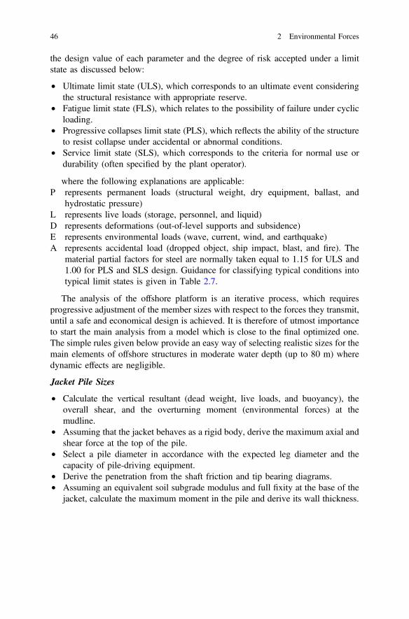
the design value of each parameter and the degree of risk accepted under a limitstate as discussed below:
• Ultimate limit state (ULS), which corresponds to an ultimate event consideringthe structural resistance with appropriate reserve.
• Fatigue limit state (FLS), which relates to the possibility of failure under cyclicloading.
• Progressive collapses limit state (PLS), which reflects the ability of the structureto resist collapse under accidental or abnormal conditions.
• Service limit state (SLS), which corresponds to the criteria for normal use ordurability (often specified by the plant operator).
where the following explanations are applicable:P represents permanent loads (structural weight, dry equipment, ballast, and
hydrostatic pressure)L represents live loads (storage, personnel, and liquid)D represents deformations (out-of-level supports and subsidence)E represents environmental loads (wave, current, wind, and earthquake)A represents accidental load (dropped object, ship impact, blast, and fire). The
material partial factors for steel are normally taken equal to 1.15 for ULS and1.00 for PLS and SLS design. Guidance for classifying typical conditions intotypical limit states is given in Table 2.7.
The analysis of the offshore platform is an iterative process, which requiresprogressive adjustment of the member sizes with respect to the forces they transmit,until a safe and economical design is achieved. It is therefore of utmost importanceto start the main analysis from a model which is close to the final optimized one.The simple rules given below provide an easy way of selecting realistic sizes for themain elements of offshore structures in moderate water depth (up to 80 m) wheredynamic effects are negligible.
Jacket Pile Sizes
• Calculate the vertical resultant (dead weight, live loads, and buoyancy), theoverall shear, and the overturning moment (environmental forces) at themudline.
• Assuming that the jacket behaves as a rigid body, derive the maximum axial andshear force at the top of the pile.
• Select a pile diameter in accordance with the expected leg diameter and thecapacity of pile-driving equipment.
• Derive the penetration from the shaft friction and tip bearing diagrams.• Assuming an equivalent soil subgrade modulus and full fixity at the base of the
jacket, calculate the maximum moment in the pile and derive its wall thickness.
46 2 Environmental Forces
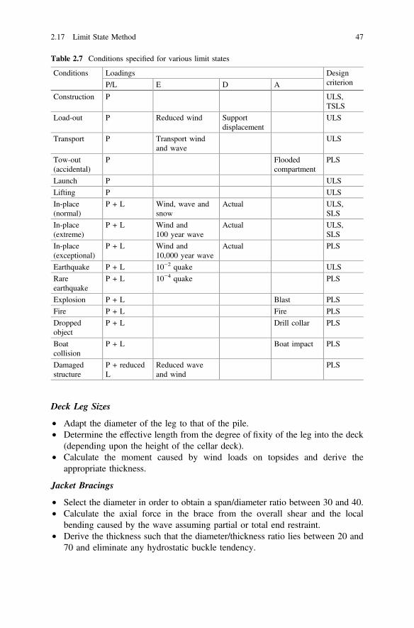
Deck Leg Sizes
• Adapt the diameter of the leg to that of the pile.• Determine the effective length from the degree of fixity of the leg into the deck
(depending upon the height of the cellar deck).• Calculate the moment caused by wind loads on topsides and derive the
appropriate thickness.
Jacket Bracings
• Select the diameter in order to obtain a span/diameter ratio between 30 and 40.• Calculate the axial force in the brace from the overall shear and the local
bending caused by the wave assuming partial or total end restraint.• Derive the thickness such that the diameter/thickness ratio lies between 20 and
70 and eliminate any hydrostatic buckle tendency.
Table 2.7 Conditions specified for various limit states
Conditions Loadings DesigncriterionP/L E D A
Construction P ULS,TSLS
Load-out P Reduced wind Supportdisplacement
ULS
Transport P Transport windand wave
ULS
Tow-out(accidental)
P Floodedcompartment
PLS
Launch P ULS
Lifting P ULS
In-place(normal)
P + L Wind, wave andsnow
Actual ULS,SLS
In-place(extreme)
P + L Wind and100 year wave
Actual ULS,SLS
In-place(exceptional)
P + L Wind and10,000 year wave
Actual PLS
Earthquake P + L 10−2 quake ULS
Rareearthquake
P + L 10−4 quake PLS
Explosion P + L Blast PLS
Fire P + L Fire PLS
Droppedobject
P + L Drill collar PLS
Boatcollision
P + L Boat impact PLS
Damagedstructure
P + reducedL
Reduced waveand wind
PLS
2.17 Limit State Method 47
Deck Framing
• Select spacing between stiffeners (typically 500–800 mm).• Derive the plate thickness from formulae accounting for local plastification
under the wheel footprint of the design forklift truck.• Determine by straight beam formulae the sizes of the main girders under
‘blanket’ live loads and/or the respective weight of the heaviest equipment.
The static in-place analysis is the basic and generally the simplest of all analyses.The structure is modeled as it stands during its operational life and subjected topseudo-static loads. This analysis is always carried at the very early stage of theproject, often from a simplified model, to size the main elements of the structure.The main model should account for eccentricities and local reinforcements at thejoints. For example, a typical model for North Sea jacket may feature over 800nodes and 4,000 members. The contribution of appurtenances, such as risers,J-tubes, caissons, conductors, boat-fenders, etc., to the overall stiffness of thestructure is normally neglected. They are therefore analyzed separately and theirreactions applied as loads at the interfaces with the main structure. Since theirbehavior is nonlinear, foundations are often analyzed separately from the structuralmodel. They are represented by an equivalent load-dependent secant stiffnessmatrix; coefficients are determined by an iterative process where the forces anddisplacements at the common boundaries of structural and foundation models areequated. This matrix may need to be adjusted to the mean reaction corresponding toeach loading condition. The static in-place analysis is performed under differentconditions where the loads are approximated by their pseudo-static equivalent. Thebasic loads relevant to a given condition are multiplied by the appropriate loadfactors and combined to produce the most severe effect in each individual elementof the structure. A dynamic analysis is normally mandatory for every offshorestructure, but can be restricted to the main modes in the case of stiff structures.
2.18 Fabrication and Installation Loads
These loads are temporary and arise during fabrication and installation of theplatform or its components. During fabrication, various structural componentsgenerate lifting forces, while in the installation, phase forces are generated duringplatform load-out, transportation to the site, launching and upending, as well asduring lifts related to installation. According to the Det Norske Veritas (DNV)rules, the return period for computing design environmental conditions for instal-lation and fabrication loads is three times as that of the duration of the corre-sponding phase. API-RP2A, on the other hand, leaves this design return period upto the owner, while the BS6235 rules recommend a minimum recurrence interval of10 years for the design environmental loads associated with transportation of thestructure to the offshore site.
48 2 Environmental Forces
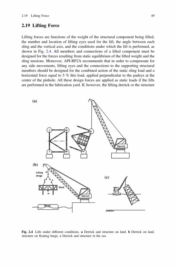
2.19 Lifting Force
Lifting forces are functions of the weight of the structural component being lifted,the number and location of lifting eyes used for the lift, the angle between eachsling and the vertical axis, and the conditions under which the lift is performed, asshown in Fig. 2.4. All members and connections of a lifted component must bedesigned for the forces resulting from static equilibrium of the lifted weight and thesling tensions. Moreover, API-RP2A recommends that in order to compensate forany side movements, lifting eyes and the connections to the supporting structuralmembers should be designed for the combined action of the static sling load and ahorizontal force equal to 5 % this load, applied perpendicular to the padeye at thecenter of the pinhole. All these design forces are applied as static loads if the liftsare performed in the fabrication yard. If, however, the lifting derrick or the structure
Fig. 2.4 Lifts under different conditions. a Derrick and structure on land. b Derrick on land,structure on floating barge. c Derrick and structure in the sea
2.19 Lifting Force 49
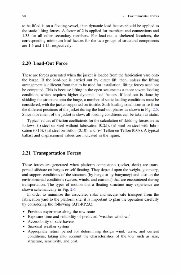
to be lifted is on a floating vessel, then dynamic load factors should be applied tothe static lifting forces. A factor of 2 is applied for members and connections and1.35 for all other secondary members. For load-out at sheltered locations, thecorresponding minimum load factors for the two groups of structural componentsare 1.5 and 1.15, respectively.
2.20 Load-Out Force
These are forces generated when the jacket is loaded from the fabrication yard ontothe barge. If the load-out is carried out by direct lift, then, unless the liftingarrangement is different from that to be used for installation, lifting forces need notbe computed. This is because lifting in the open sea creates a more severe loadingcondition, which requires higher dynamic load factors. If load-out is done byskidding the structure onto the barge, a number of static loading conditions must beconsidered, with the jacket supported on its side. Such loading conditions arise fromthe different positions of the jacket during the load-out phases as shown in Fig. 2.5.Since movement of the jacket is slow, all loading conditions can be taken as static.
Typical values of friction coefficients for the calculation of skidding forces are asfollows: (i) steel on steel without lubrication (0.25); (ii) steel on steel with lubri-cation (0.15); (iii) steel on Teflon (0.10); and (iv) Teflon on Teflon (0.08). A typicalballast and displacement values are indicated in the figure.
2.21 Transportation Forces
These forces are generated when platform components (jacket, deck) are trans-ported offshore on barges or self-floating. They depend upon the weight, geometry,and support conditions of the structure (by barge or by buoyancy) and also on theenvironmental conditions (waves, winds, and currents) that are encountered duringtransportation. The types of motion that a floating structure may experience areshown schematically in Fig. 2.6.
In order to minimize the associated risks and secure safe transport from thefabrication yard to the platform site, it is important to plan the operation carefullyby considering the following (API-RP2A):
• Previous experience along the tow route• Exposure time and reliability of predicted ‘weather windows’• Accessibility of safe havens• Seasonal weather system• Appropriate return period for determining design wind, wave, and current
conditions, taking into account the characteristics of the tow such as size,structure, sensitivity, and cost.
50 2 Environmental Forces
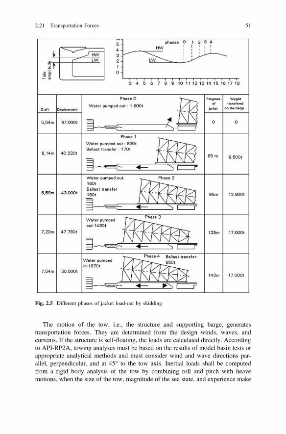
The motion of the tow, i.e., the structure and supporting barge, generatestransportation forces. They are determined from the design winds, waves, andcurrents. If the structure is self-floating, the loads are calculated directly. Accordingto API-RP2A, towing analyses must be based on the results of model basin tests orappropriate analytical methods and must consider wind and wave directions par-allel, perpendicular, and at 45° to the tow axis. Inertial loads shall be computedfrom a rigid body analysis of the tow by combining roll and pitch with heavemotions, when the size of the tow, magnitude of the sea state, and experience make
Fig. 2.5 Different phases of jacket load-out by skidding
2.21 Transportation Forces 51
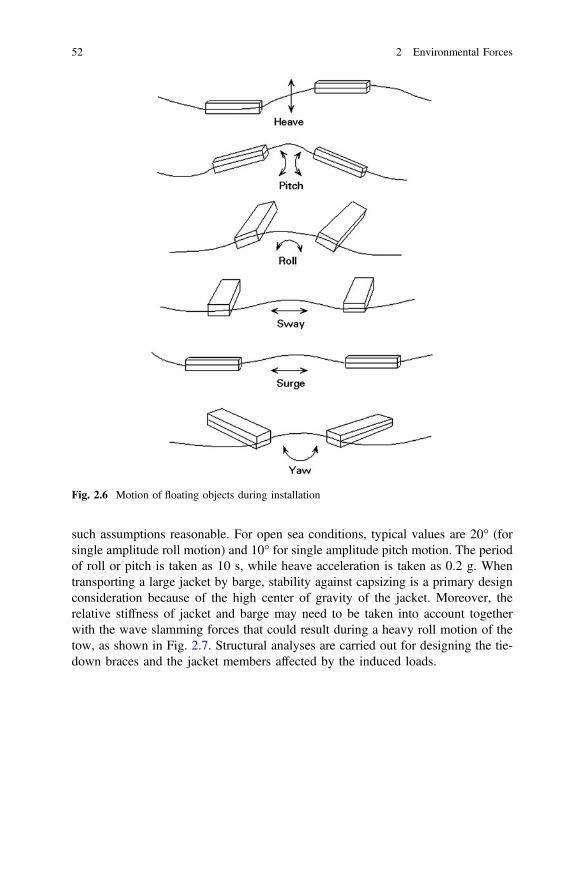
such assumptions reasonable. For open sea conditions, typical values are 20° (forsingle amplitude roll motion) and 10° for single amplitude pitch motion. The periodof roll or pitch is taken as 10 s, while heave acceleration is taken as 0.2 g. Whentransporting a large jacket by barge, stability against capsizing is a primary designconsideration because of the high center of gravity of the jacket. Moreover, therelative stiffness of jacket and barge may need to be taken into account togetherwith the wave slamming forces that could result during a heavy roll motion of thetow, as shown in Fig. 2.7. Structural analyses are carried out for designing the tie-down braces and the jacket members affected by the induced loads.
Fig. 2.6 Motion of floating objects during installation
52 2 Environmental Forces
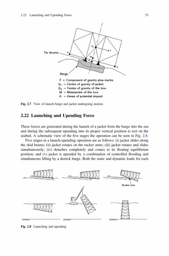
2.22 Launching and Upending Force
These forces are generated during the launch of a jacket from the barge into the seaand during the subsequent upending into its proper vertical position to rest on theseabed. A schematic view of the five stages the operation can be seen in Fig. 2.8.
Five stages in a launch-upending operation are as follows: (i) jacket slides alongthe skid beams; (ii) jacket rotates on the rocker arms; (iii) jacket rotates and slidessimultaneously; (iv) detaches completely and comes to its floating equilibriumposition; and (v) jacket is upended by a combination of controlled flooding andsimultaneous lifting by a derrick barge. Both the static and dynamic loads for each
Fig. 2.7 View of launch barge and jacket undergoing motion
Fig. 2.8 Launching and upending
2.22 Launching and Upending Force 53
stage of the above under the action of wind, waves, and current need to be includedin the analysis.
To start the launch, the barge must be ballasted to an appropriate draft and trimangle and subsequently the jacket must be pulled toward the stern by a winch.Sliding of the jacket starts as soon as the downward force (gravity component andwinch pull) exceeds the friction force. As the jacket slides, its weight is supportedon the two legs that are part of the launch trusses. The support length keepsdecreasing and reaches a minimum, equal to the length of the rocker beams, whenrotation starts. It is generally at this instant that the most severe launching forcesdevelop as reactions to the weight of the jacket. During the last two stages, variablehydrostatic forces arise, which have to be considered at all members affected.Buoyancy calculations are required for every stage of the operation to ensure fullycontrolled, stable motion. Computer programs are available to perform the stressanalyses required for launching and upending and also to portray the whole oper-ation graphically.
2.23 Accidental Load
According to the DNV rules, accidental loads are ill-defined with respect tointensity and frequency, which may occur as a result of an accident or exceptionalcircumstances. Examples of accidental loads are loads due to collision with vessels,fire or explosion, dropped objects, and unintended flooding of buoyancy tanks.Special measures are normally taken to reduce the risk from accidental loads. Forexample, protection of wellheads or other critical equipment from a dropped objectcan be provided by specially designed, impact resistant covers. An accidental loadcan be disregarded if its annual probability of occurrence is less than 10−4. Thisnumber is the estimate of order of magnitude and is extremely difficult to compute.
Exercise
1. The design stages of various offshore platform are _________, ___________,and ______________.
2. The data collected during the FEED stage will be further verified to make surethe _________ and _________ of such data for further use.
3. Loads on offshore structures are ____________ and ___________.4. Gravity loads are arising from _________ and __________either permanent or
temporary.5. Seismic loads are arising from derived type ___________.6. Gravity loads are _____________, ______________, _____________,
______________, and ___________.
54 2 Environmental Forces

7. Environmental loads are _____________, ______________, _____________,______________, __________, and ___________.
8. The fluid loads are weight of fluid on the platform during _______________.9. The wind speed at 10 m above ________________ is normally provided (V0).
10. Wind speed obtained shall be ____________ to the height above for the cal-culation of wind speed.
11. The wind speed may be classified as ____________ and ________________.12. ____________ are measured in an average less than 1 min in duration.13. Wind loads shall be calculated as per ___________ guidelines.14. Wind-driven waves are a major source of ______________on offshore
platforms.15. Sustained wind speeds measured for ______________ duration shall be used to
compute global platform wind loads and gust wind which is measured for_________ duration shall be used to compute the wind loads to design indi-vidual members.
16. The wind pressure can be calculated as fw = ___________________.17. The total force on the platform can be calculated as Fx = ______________.18.
Calculate wind load on oblique directions Fθ =19. In_____________________, a discrete set of design waves (maximum) and
associated periods will be selected to generate loads on the structure.20. In the spectral method, an energy spectrum of the sea state for the location will
be taken and a ___________________ for the response will be generated.21. Transfer function will be used to compute the ___________ in the structural
members.22. Sea-state energy spectra available for use are ________, ___________, and
___________.23. Tides may be classified as___________, _____________, and
_________________.24. Combination of astronomical tide, wind tide, and pressure differential tide are
called ____________.25. The forces exerted by waves are most dominant in governing the jacket
structures design especially the______________.
Exercise 55

26. The wave loads exerted on the jacket is applied laterally on all members, and itgenerates __________________ on the structure.
27. Period of wind-generated waves in the open sea can be in the order of_______________.
28. Waves are called ______________ and contain most part of ____________.29. Relationship between significant wave height (Hs) and the maximum wave
height (Hmax) is ____________________.30. Match the design wave height for various regions is tabulated below:
I. Bay of Bengal (a) 11 m for 1 year and 24 m for 100 years
II. Gulf of Mexico (b) 6 m for 1 year and 12 m for 100 years
III. South China Sea (c) 5 m for 1 year and 12 m for 100 years
IV. Arabian Sea (d) 14 m for 1 year and 22 m for 100 years
V. Gulf of Thailand (e) 12 m for 1 year and 24 m for 100 years
VI. Persian Gulf (f) 8 m for 1 year and 18 m for 100 years
VII. North Sea (g) 8 m for 1 year and 18 m for 100 years
31. Draw the current profile of wave-driven currents and tidal currents.32. Name some standard spectrum available in the literature.33. Ocean currents are classified into few types based on their nature they are
_______________, __________________, and______________________________.
34. Write down the expression for current variation along the depth and explain theterms involved in it.
35. Marine growth is an important part in increasing the loads on________________.
36. Growth of marine algae increases the ______________ and__________________which in turn increase the wave or current loading.
37. The thickness of marine growth generally _____________ with depth from themean sea level, and it is maximum in the _____________.
38. Splash Zone is a region where the water levels _______________ between lowto high.
39. Write down the expression for Morison equation and explain the termsappropriately.
40. Algebraic sum of wave and current loads is different from calculation of loadby adding the horizontal water particle velocity with the current velocity andcomputing the loads. This is because of____________________________________________.
41. Interaction between the wave and current modifies the____________________________.
42. Name some wave theories.43. API-RP2A recommends to use a chart for such selection based on
___________ and ______________.44. The reserve buoyancy is defined as buoyancy in ______________________.
56 2 Environmental Forces

45. The buoyancy force can be calculated using ________________method and______________ method.
46. Sketch a jacket structure and mark the MSL, LAT, and HAT in the jacketstructure.
47. Write down the empirical equation to estimate the force Fice.48. Platforms located in the vicinity of the river mouth will be subjected to
______________.49. Write down the empirical equation to estimate the force Fmud.50. Scour is removal of seafloor soils caused by ____________ and
__________________.51. Explain the force regime.52. P-M spectral method describes the fully developed sea determined by
_______________ parameter that is __________________.53. In P-M spectrum, fetch and duration are considered _____________.54. ______________________spectrum is on basis of the assumption that the
spectrum is narrow banded, and individual wave height and wave period followRayleigh distribution.
55. ISSC spectrum suggested modification in form of the___________________________.
56. _____________________ proposed modification in the P-M spectrum in termsof ________________________ and ____________________.
57. Write down the expression for Morison equation for force per unit lengthexperienced by the structure due to its motion through the water.
58. Site-dependent databases are being developed to characterize the time varyingfluid induced loads of ________, ___________, and ______________.
59. Explain the linear wave theory with the neat sketch and write the expression forvelocity potential.
60. List the assumptions based on which the Morison equation is derived.
Answers
1. front end engineering design (FEED) or concept selection; basic design;detailed design
2. authenticity and reliability3. gravity loads and environmental loads4. dead weight of structure and facilities5. gravity loads6. structural dead loads; facility dead loads; fluid loads; live loads; and drilling
loads7. wind loads; wave loads; current loads; buoyancy loads; ice loads; and mud
loads8. operation
Exercise 57
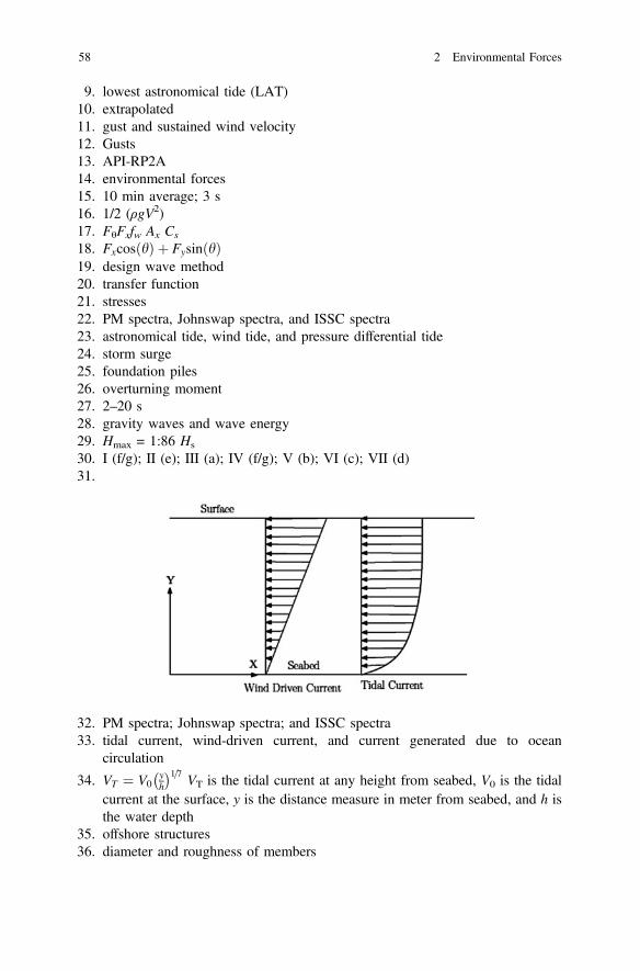
9. lowest astronomical tide (LAT)10. extrapolated11. gust and sustained wind velocity12. Gusts13. API-RP2A14. environmental forces15. 10 min average; 3 s16. 1/2 (ρgV2)17. FθFxfw Ax Cs
18. FxcosðhÞ þ FysinðhÞ19. design wave method20. transfer function21. stresses22. PM spectra, Johnswap spectra, and ISSC spectra23. astronomical tide, wind tide, and pressure differential tide24. storm surge25. foundation piles26. overturning moment27. 2–20 s28. gravity waves and wave energy29. Hmax = 1:86 Hs
30. I (f/g); II (e); III (a); IV (f/g); V (b); VI (c); VII (d)31.
32. PM spectra; Johnswap spectra; and ISSC spectra33. tidal current, wind-driven current, and current generated due to ocean
circulation
34. VT ¼ V0yh
� �1=7VT is the tidal current at any height from seabed, V0 is the tidal
current at the surface, y is the distance measure in meter from seabed, and h isthe water depth
35. offshore structures36. diameter and roughness of members
58 2 Environmental Forces
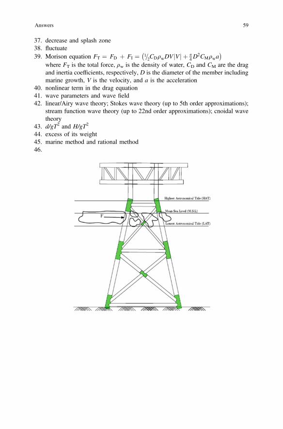
37. decrease and splash zone38. fluctuate39. Morison equation FT ¼ FD þ FI ¼ 1=2CDqwDV Vj j þ p
4D2CMqwa
� �where FT is the total force, ρw is the density of water, CD and CM are the dragand inertia coefficients, respectively, D is the diameter of the member includingmarine growth, V is the velocity, and a is the acceleration
40. nonlinear term in the drag equation41. wave parameters and wave field42. linear/Airy wave theory; Stokes wave theory (up to 5th order approximations);
stream function wave theory (up to 22nd order approximations); cnoidal wavetheory
43. d/gT2 and H/gT2
44. excess of its weight45. marine method and rational method46.
Answers 59
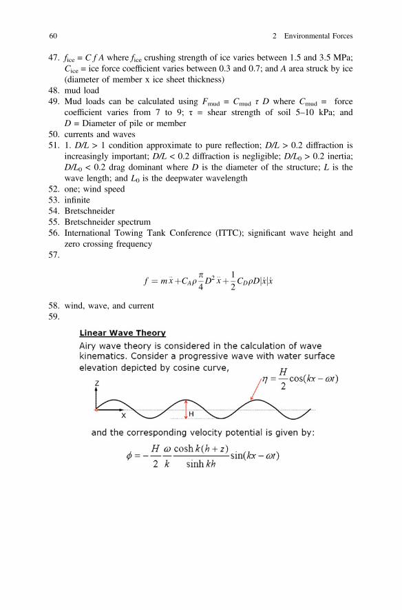
47. fice = C f A where fice crushing strength of ice varies between 1.5 and 3.5 MPa;Cice = ice force coefficient varies between 0.3 and 0.7; and A area struck by ice(diameter of member x ice sheet thickness)
48. mud load49. Mud loads can be calculated using Fmud = Cmud τ D where Cmud = force
coefficient varies from 7 to 9; τ = shear strength of soil 5–10 kPa; andD = Diameter of pile or member
50. currents and waves51. 1. D/L > 1 condition approximate to pure reflection; D/L > 0.2 diffraction is
increasingly important; D/L < 0.2 diffraction is negligible; D/L0 > 0.2 inertia;D/L0 < 0.2 drag dominant where D is the diameter of the structure; L is thewave length; and L0 is the deepwater wavelength
52. one; wind speed53. infinite54. Bretschneider55. Bretschneider spectrum56. International Towing Tank Conference (ITTC); significant wave height and
zero crossing frequency57.
f ¼ mx::þCAq
p4D2 x
::þ 12CDqDj _xj _x
58. wind, wave, and current59.
60 2 Environmental Forces

60. Assumptions are as follows:
• Flow is assumed to be not disturbed by the presence of the structure.• Force calculation is empirical calibrated by experimental results.• Suitable coefficients need to be used depending on the shape of the body or
structure.• Validity range shall be checked before use and generally suitable for most
jacket type structures where D/L ≪ 0.2 where D is the diameter of thestructural member and L is the wave length.
Answers 61
Chapter 3Introduction to Structural Dynamics
Abstract This chapter deals with introduction to structural dynamics and itsapplication to offshore structures. Basics of single degree of freedom are discussedto highlight the conventional mathematical model of single degree of freedom. Freevibration analysis and forced vibration analysis are discussed with focus on fewimportant dynamic characteristics of the single-degree-of-freedom and multi-degrees-of-freedom models. Solved numerical examples of determining naturalfrequencies and mode shapes of different mathematical model of single-degree-of-freedom and multi-degrees-of-freedom systems are included.
Keywords Single-degree-of-freedom � Multi-degrees-of-freedom � Un-dampedfree vibration � Forced vibration � Structural damping � Half power method �Influence coefficient method � Dunkerley’s method � Stodla method � Modesuperposition � Mode truncation � Static correction
3.1 Introduction
For understanding the advantages of the offshore structural forms and action, it isnecessary to convert the structure into simple basic mathematical models fordynamic analysis. However, it is important to note that complexities arising fromthe mechanical and process equipment that forms a major part of topside activity ofoffshore structures pose serious limitation to such idealized mathematical modelsconsidered for dynamic analysis. Dynamic loads are defined as time-varying loadswhose magnitude, direction of application, or position vary continuously with time.As repose to these applied loads, response of the structure also varies with respectto time. Basic approaches to evaluate the response of structures to such dynamicloads are (i) deterministic and (ii) non-deterministic. In deterministic approach, inwhich the time history of the loading is fully known with the highly varying andirregular load magnitude, loading can be classified as prescribed dynamic loading.In non-deterministic approach, in which the time history of the loading is not
© Springer India 2015S. Chandrasekaran, Dynamic Analysis and Design of Offshore Structures,Ocean Engineering & Oceanography 5, DOI 10.1007/978-81-322-2277-4_3
63
completely known but can be defined in statistical sense, the loading is termed asrandom dynamic loading. Deterministic analyses lead to displacement time historycorresponding to the given (completely known) load time history. Other aspectssuch as stress, strain, and internal forces are derived from the established dis-placement patterns. In case of non-deterministic analyses, results obtained willprovide statistical information of the displacement pattern under the action of astatistically defined loading (random loads). Other aspects such as stress, strain, andinternal forces such as bending moment and shear shall be computed directly bysimilar independent non-deterministic analyses rather than from deriving them fromthe displacement results as in the earlier case.
Essential characteristics of dynamic loading are their time-varying nature andpresence of inertia force. Inertia force is the force, which resists acceleration, whichis the most essential characteristic of dynamic analysis as they represent a signif-icant portion of the total load. As the applied load is time-varying, dynamic analysisis never a single solution like static analysis and the response is then evaluated.
3.2 Fundamentals of Structural Dynamics
All bodies having mass and elasticity are capable of vibration. Mass is an inherentproperty of a body, and elasticity causes relative motion of the parts. Due to anexternal force, the body gets vibrated, and the internal inherent forces in the form ofelastic energy are developed, and this tries to bring back the structure to its originalposition. At equilibrium, the total energy is converted to kinetic energy, and then, thebody continues to move in the opposite direction. Then, kinetic energy is convertedinto strain or elastic energy due to which the body returns to its equilibrium position.By this way, the vibratory motion is repeated indefinitely with the exchange ofenergy. Thus, any motion, which repeats itself after an interval of time, is calledvibration. The major factors that cause vibration are the unbalanced centrifugal forcein the system, elastic property of the system, and external excitation.
Before getting into the subject, it is necessary to understand some terminologies.A motion, which repeats itself after an equal interval of time, is called periodicmotion. The time taken to complete one cycle is called the time period, and thenumber of cycles per unit time is called frequency. Free vibrations are the vibrationswhich are caused due to initial displacement with the absence of an external force,and their frequency is called natural frequency. The mode, which has the lowestnatural frequency, is called the fundamental mode of vibration. When the frequencyof the external vibration matches with the natural frequency of a vibrating body, theamplitude of vibration becomes excessively large, and this is known as resonance.Degree of freedom is defined as the number of independent displacement compo-nents of a structural system that are necessary at any given time to represent the effectof all significant inertia forces present in the system. Systems, which have infinitenumber of degrees of freedom, are called continuous systems, and systems with finitenumber of degrees of freedom are called discrete or lumped systems.
64 3 Introduction to Structural Dynamics
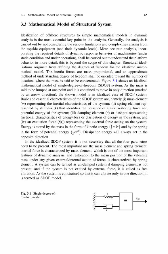
3.3 Mathematical Model of Structural System
Idealization of offshore structures to simple mathematical models in dynamicanalysis is the most essential key point in the analysis. Generally, the analysis iscarried out by not considering the serious limitations and complexities arising fromthe topside equipment (and their dynamic loads). More accurate analysis, incor-porating the required details of dynamic response behavior of machineries (understatic condition and under operation), shall be carried out to understand the platformbehavior in more detail; this is beyond the scope of this chapter. Structural ideal-izations originate from defining the degrees of freedom for the idealized mathe-matical model. The inertia forces are mass proportional, and an approximatemethod of understanding degree of freedom shall be oriented toward the number oflocations where the mass is said to be concentrated. Figure 3.1 shows an idealizedmathematical model of single-degree-of-freedom (SDOF) system. As the mass issaid to be lumped at one point and it is contained to move in only direction (markedby an arrow direction), the shown model is an idealized case of SDOF system.Basic and essential characteristics of the SDOF system are, namely (i) mass element(m) representing the inertial characteristics of the system; (ii) spring element rep-resented by stiffness (k) that identifies the presence of elastic restoring force andpotential energy of the system; (iii) damping element (c) or dashpot representingfrictional characteristics of energy loss or dissipation of energy in the system; and(iv) an excitation force (f(t)) representing the external force acting on the system.Energy is stored by the mass in the form of kinetic energy 1
2m _x2� �
and by the springin the form of potential energy 1
2 kx2
� �. Dissipation energy will always act in the
opposite direction.In the idealized SDOF system, it is not necessary that all the four parameters
need to be present. The most important are the mass element and spring element;inertial force is characterized by mass element, which is one of the most importantfeatures of dynamic analysis, and restoration to the mean position of the vibratingmass under any given external/internal action of forces is characterized by springelement. A system can be termed as un-damped system if damping element is notpresent, and if the system is not excited by external force, it is called as freevibration. As the system is constrained so that it can vibrate only in one direction, itis termed as SDOF model.
Fig. 3.1 Single-degree-of-freedom model
3.3 Mathematical Model of Structural System 65
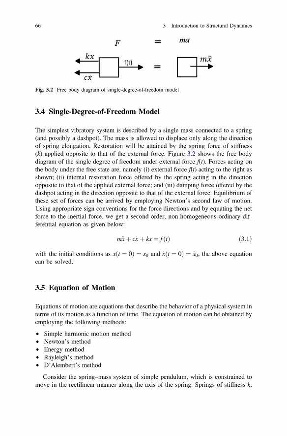
3.4 Single-Degree-of-Freedom Model
The simplest vibratory system is described by a single mass connected to a spring(and possibly a dashpot). The mass is allowed to displace only along the directionof spring elongation. Restoration will be attained by the spring force of stiffness(k) applied opposite to that of the external force. Figure 3.2 shows the free bodydiagram of the single degree of freedom under external force f(t). Forces acting onthe body under the free state are, namely (i) external force f(t) acting to the right asshown; (ii) internal restoration force offered by the spring acting in the directionopposite to that of the applied external force; and (iii) damping force offered by thedashpot acting in the direction opposite to that of the external force. Equilibrium ofthese set of forces can be arrived by employing Newton’s second law of motion.Using appropriate sign conventions for the force directions and by equating the netforce to the inertial force, we get a second-order, non-homogeneous ordinary dif-ferential equation as given below:
m€xþ c _xþ kx ¼ f ðtÞ ð3:1Þ
with the initial conditions as x t ¼ 0ð Þ ¼ x0 and _xðt ¼ 0Þ ¼ _x0, the above equationcan be solved.
3.5 Equation of Motion
Equations of motion are equations that describe the behavior of a physical system interms of its motion as a function of time. The equation of motion can be obtained byemploying the following methods:
• Simple harmonic motion method• Newton’s method• Energy method• Rayleigh’s method• D’Alembert’s method
Consider the spring–mass system of simple pendulum, which is constrained tomove in the rectilinear manner along the axis of the spring. Springs of stiffness k,
Fig. 3.2 Free body diagram of single-degree-of-freedom model
66 3 Introduction to Structural Dynamics
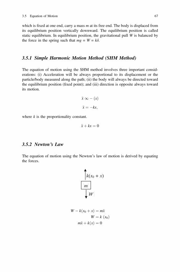
which is fixed at one end, carry a mass m at its free end. The body is displaced fromits equilibrium position vertically downward. The equilibrium position is calledstatic equilibrium. In equilibrium position, the gravitational pull W is balanced bythe force in the spring such that mg = W = kδ.
3.5.1 Simple Harmonic Motion Method (SHM Method)
The equation of motion using the SHM method involves three important consid-erations: (i) Acceleration will be always proportional to its displacement or theparticle/body measured along the path; (ii) the body will always be directed towardthe equilibrium position (fixed point); and (iii) direction is opposite always towardits motion.
€x 1� ðxÞ
€x ¼ �kx;
where k is the proportionality constant.
€xþ kx ¼ 0
3.5.2 Newton’s Law
The equation of motion using the Newton’s law of motion is derived by equatingthe forces.
W � kðx0 þ xÞ ¼ m€x
W ¼ k ðx0Þm€xþ k xð Þ ¼ 0
3.5 Equation of Motion 67
3.5.3 Energy Method
In a conservative system, the total sum of the energy is constant. In the vibratorysystem, the energy is partly potential and partly constant. The kinetic energy is afunction of the velocity, and the potential energy is a function of displacement.
K:E: ¼ 12m _x2
P:E: ¼ 12kx2
ddt
12m _x2 þ 1
2kx2
� �¼ 0
_x m€xþ kx½ � ¼ 0
m€xþ kx ¼ 0
3.5.4 Rayleigh’s Method
It is assumed that maximum kinetic energy at the mean position is equal to themaximum potential energy at the extreme position. If the motion is assumed to besimple harmonic, then
x ¼ A sinxnt
where x = displacement of the body from mean position to the extreme position.
_x ¼ xnA cosxnt
Maximum velocity at mean position
_x ¼ Axn
So, maximum kinetic energy at the mean position = 12m _x2 ¼ 1
2mx2nA
2
Maximum kinetic energy at the extreme position = 12 kA
2
12mx2
nA2 ¼ 1
2kA2
xn ¼ffiffiffiffikm
r
These methods are widely used for the determination of the natural frequency of thesystem.
68 3 Introduction to Structural Dynamics
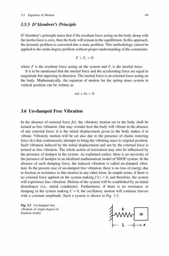
3.5.5 D’Alembert’s Principle
D’Alembert’s principle states that if the resultant force acting on the body along withthe inertia force is zero, then the body will remain in the equilibrium. In this approach,the dynamic problem is converted into a static problem. This methodology cannot beapplied to the multi-degree problem without proper understanding of the constraints.
F þ Fi ¼ 0
where F is the resultant force acting on the system and Fi is the inertial force.It is to be mentioned that the inertial force and the accelerating force are equal in
magnitude but opposing in direction. The inertial force is an external force acting onthe body. Mathematically, the equation of motion for the spring–mass system invertical position can be written as
m€xþ kx ¼ 0
3.6 Un-damped Free Vibration
In the absence of external force f(t), the vibratory motion set in the body shall betermed as free vibration. One may wonder how the body will vibrate in the absenceof any external force; it is the initial displacement given to the body makes it tovibrate. Vibratory motion will be set also due to the presence of elastic restoringforce (kx) that continuously attempts to bring the vibrating mass to original position.Such vibration induced by the initial displacement and not by the external force istermed as free vibration. The whole action of restoration may also be influenced bythe presence of dashpot in the system. As explained earlier, there is no necessity ofthe presence of dashpot in an idealized mathematical model of SDOF system. In theabsence of such damping force, the induced vibration is called un-damped vibra-tion. In the present case of un-damped free vibration, there is no loss of energy dueto friction or resistance to this motion in any other form. In simple terms, if there isno external force applied on the system making f ðtÞ ¼ 0, and therefore, the systemwill experience free vibration. Motion of the system will be established by an initialdisturbance (i.e., initial conditions). Furthermore, if there is no resistance ordamping in the system making C = 0, the oscillatory motion will continue foreverwith a constant amplitude. Such a system is shown in Fig. 3.3.
Fig. 3.3 Un-damped freevibration of single-degree-of-freedom model
3.5 Equation of Motion 69
Based on the free body diagram explained earlier, equation of motion forun-damped free system can be written as follows:
m€xþ kx ¼ 0 ð3:2Þ
Dividing by mass throughout, we get the following form:
€xþ km¼ 0
€xþ x2 ¼ 0
where
x2 ¼ km
For the second-order differential equation as shown above, auxiliary equation isgiven as follows:
D2 þ x2 ¼ 0
D ¼ �ix
Complimentary function is given as follows:
xðtÞ ¼ C1 cosxt þ C2 sinxt ð3:3Þ
Using the initial condition as explained earlier, the above equation reduces to thefollowing form:
xðtÞ ¼ x0 cosxt þ _x0xsinxt ð3:4Þ
where x0 and _x0 are initial displacements and velocities, respectively, and ωn is thenatural frequency of the said vibrating motion. It can be easily seen that the naturalfrequency is dependent on the mass of the system and spring constant or restoringforce coefficient of the system; it is independent of the said initial displacementgiven to preset the vibrating motion to the body.
3.7 Damped Free Vibration
While discussing the above case of free vibration of SDOF model, one may wonderabout the duration of such vibration being setup by the given initial displacement.The duration of such vibration is hypothetically infinite, as no external (or) internalagency is responsible to control such induced vibration. But in practice, one can
70 3 Introduction to Structural Dynamics
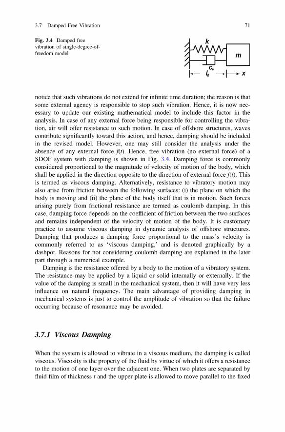
notice that such vibrations do not extend for infinite time duration; the reason is thatsome external agency is responsible to stop such vibration. Hence, it is now nec-essary to update our existing mathematical model to include this factor in theanalysis. In case of any external force being responsible for controlling the vibra-tion, air will offer resistance to such motion. In case of offshore structures, wavescontribute significantly toward this action, and hence, damping should be includedin the revised model. However, one may still consider the analysis under theabsence of any external force f(t). Hence, free vibration (no external force) of aSDOF system with damping is shown in Fig. 3.4. Damping force is commonlyconsidered proportional to the magnitude of velocity of motion of the body, whichshall be applied in the direction opposite to the direction of external force f(t). Thisis termed as viscous damping. Alternatively, resistance to vibratory motion mayalso arise from friction between the following surfaces: (i) the plane on which thebody is moving and (ii) the plane of the body itself that is in motion. Such forcesarising purely from frictional resistance are termed as coulomb damping. In thiscase, damping force depends on the coefficient of friction between the two surfacesand remains independent of the velocity of motion of the body. It is customarypractice to assume viscous damping in dynamic analysis of offshore structures.Damping that produces a damping force proportional to the mass’s velocity iscommonly referred to as ‘viscous damping,’ and is denoted graphically by adashpot. Reasons for not considering coulomb damping are explained in the laterpart through a numerical example.
Damping is the resistance offered by a body to the motion of a vibratory system.The resistance may be applied by a liquid or solid internally or externally. If thevalue of the damping is small in the mechanical system, then it will have very lessinfluence on natural frequency. The main advantage of providing damping inmechanical systems is just to control the amplitude of vibration so that the failureoccurring because of resonance may be avoided.
3.7.1 Viscous Damping
When the system is allowed to vibrate in a viscous medium, the damping is calledviscous. Viscosity is the property of the fluid by virtue of which it offers a resistanceto the motion of one layer over the adjacent one. When two plates are separated byfluid film of thickness t and the upper plate is allowed to move parallel to the fixed
Fig. 3.4 Damped freevibration of single-degree-of-freedom model
3.7 Damped Free Vibration 71
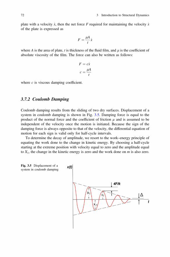
plate with a velocity _x, then the net force F required for maintaining the velocity _xof the plate is expressed as
F ¼ lAt_x
where A is the area of plate, t is thickness of the fluid film, and l is the coefficient ofabsolute viscosity of the film. The force can also be written as follows:
F ¼ c_x
c ¼ lAt
where c is viscous damping coefficient.
3.7.2 Coulomb Damping
Coulomb damping results from the sliding of two dry surfaces. Displacement of asystem in coulomb damping is shown in Fig. 3.5. Damping force is equal to theproduct of the normal force and the coefficient of friction µ and is assumed to beindependent of the velocity once the motion is initiated. Because the sign of thedamping force is always opposite to that of the velocity, the differential equation ofmotion for each sign is valid only for half-cycle intervals.
To determine the decay of amplitude, we resort to the work–energy principle ofequating the work done to the change in kinetic energy. By choosing a half-cyclestarting at the extreme position with velocity equal to zero and the amplitude equalto X1, the change in the kinetic energy is zero and the work done on m is also zero.
Fig. 3.5 Displacement of asystem in coulomb damping
72 3 Introduction to Structural Dynamics
12k X2
1 � X2�1
� �� Fd X1 þ X�1ð Þ ¼ 0
or
12k X1 þ X�1ð Þ ¼ Fd
where X−1 is the amplitude after the half-cycle as shown in Fig. 3.5. By repeatingthis procedure for the next half-cycle, a further decrease in amplitude of 2Fd=k willbe found, so that the decay in amplitude per cycle is a constant and is given asfollows:
X1 � X2 ¼ 4Fd
k
The motion will cease when the amplitude becomes less than D; at this position,spring force is insufficient to overcome the static friction force, which is generallygreater than the kinetic friction force. It can also be shown that the frequency ofoscillation is the same as that of the un-damped system. Amplitude of the coulombdamping system decays linearly with time. For damped free vibration of SDOFsystem, equation of motion is given as follows:
m€xþ c _xþ kx ¼ 0 ð3:5Þ
This is a second-order, homogeneous, ordinary differential equation (ODE). If allparameters (mass, spring stiffness, and viscous damping) are constants, then theequation becomes linear with constant coefficients that can be solved by a simplecharacteristic equation method. The characteristic equation for this problem is givenas follows:
ms2 þ csþ k ¼ 0 ð3:6Þ
This determines two independent roots that fall into one of the following threecases:
1. If c2 � 4mk\0, the system is termed under-damped. The roots of the charac-teristic equation are complex conjugates, corresponding to oscillatory motionwith an exponential decay in amplitude.
2. If c2 � 4mk ¼ 0, the system is termed critically damped. The roots of thecharacteristic equation are repeated, corresponding to simple decaying motionwith at most one overshoot of the system’s resting position.
3. If c2 � 4mk[ 0, the system is termed over-damped. The roots of the charac-teristic equation are purely real and distinct, corresponding to simple expo-nentially decaying motion.
3.7 Damped Free Vibration 73
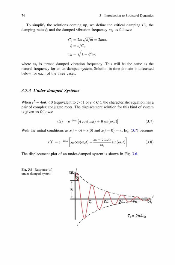
To simplify the solutions coming up, we define the critical damping Cc, thedamping ratio ξ, and the damped vibration frequency xd as follows:
Cc ¼ 2mffiffiffiffiffiffiffiffiffik=m
p¼ 2mxn
n ¼ c=Cc
xd ¼ffiffiffiffiffiffiffiffiffiffiffiffiffi1� n2
qxn
where xd is termed damped vibration frequency. This will be the same as thenatural frequency for an un-damped system. Solution in time domain is discussedbelow for each of the three cases.
3.7.3 Under-damped Systems
When c2 � 4mk\0 (equivalent to ξ < 1 or c < Cc), the characteristic equation has apair of complex conjugate roots. The displacement solution for this kind of systemis given as follows:
xðtÞ ¼ e�nxnt A cos xdtð Þ þ B sin xdtð Þ½ � ð3:7Þ
With the initial conditions as x(t = 0) = x(0) and _xðt ¼ 0Þ ¼ _x, Eq. (3.7) becomes
xðtÞ ¼ e�nxnt x0 cos xdtð Þ þ _x0 þ nxnx0xd
sin xdtð Þ� �
ð3:8Þ
The displacement plot of an under-damped system is shown in Fig. 3.6.
Fig. 3.6 Response ofunder-damped system
74 3 Introduction to Structural Dynamics
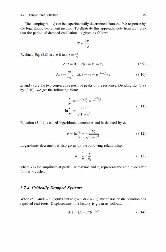
The damping ratio ξ can be experimentally determined from the free response bythe logarithmic decrement method. To illustrate this approach, note from Eq. (3.8)that the period of damped oscillations is given as follows:
T ¼ 2pxd
Evaluate Eq. (3.8) at t = 0 and t ¼ 2pxd
At t ¼ 0; xðtÞ ¼ x1 ¼ x0 ð3:9Þ
At t ¼ 2pxd
; xðtÞ ¼ x2 ¼ e�nxn2pxd x0 ð3:10Þ
x1 and x2 are the two consecutive positive peaks of the response. Dividing Eq. (3.9)by (3.10), we get the following form:
x1x2
¼ e�nxn2pxd ¼ e
2pnffiffiffiffiffiffi1�n2
p
lnx1x2
¼ 2pnffiffiffiffiffiffiffiffiffiffiffiffiffi1� n2
p ð3:11Þ
Equation (3.11) is called logarithmic decrement and is denoted by d.
d ¼ lnx1x2
¼ 2pnffiffiffiffiffiffiffiffiffiffiffiffiffi1� n2
p ð3:12Þ
Logarithmic decrement is also given by the following relationship:
d ¼ 1nln
xxn
ð3:13Þ
where x is the amplitude at particular maxima and xn represents the amplitude afterfurther n cycles.
3.7.4 Critically Damped Systems
When c2 � 4mk ¼ 0 (equivalent to ξ = 1 or c = Cc), the characteristic equation hasrepeated real roots. Displacement time history is given as follows:
xðtÞ ¼ Aþ Btð Þe�xnt ð3:14Þ
3.7 Damped Free Vibration 75
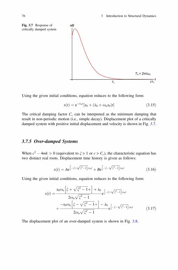
Using the given initial conditions, equation reduces to the following form:
xðtÞ ¼ e�xnt x0 þ _x0 þ xnx0ð Þt½ � ð3:15Þ
The critical damping factor Cc can be interpreted as the minimum damping thatresult in non-periodic motion (i.e., simple decay). Displacement plot of a criticallydamped system with positive initial displacement and velocity is shown in Fig. 3.7.
3.7.5 Over-damped Systems
When c2 � 4mk[ 0 (equivalent to ξ > 1 or c > Cc), the characteristic equation hastwo distinct real roots. Displacement time history is given as follows:
xðtÞ ¼ Ae �nþffiffiffiffiffiffiffiffin2�1
p xnt þ Be �n�
ffiffiffiffiffiffiffiffin2�1
p xnt ð3:16Þ
Using the given initial conditions, equation reduces to the following form:
xðtÞ ¼x0xn nþ
ffiffiffiffiffiffiffiffiffiffiffiffiffin2 � 1
pþ
h iþ _x0
2xn
ffiffiffiffiffiffiffiffiffiffiffiffiffin2 � 1
p e �nþffiffiffiffiffiffiffiffin2�1
p xnt
þ�x0xn n�
ffiffiffiffiffiffiffiffiffiffiffiffiffin2 � 1
pþ
h i� _x0
2xn
ffiffiffiffiffiffiffiffiffiffiffiffiffin2 � 1
p e �n�ffiffiffiffiffiffiffiffin2�1
p xnt ð3:17Þ
The displacement plot of an over-damped system is shown in Fig. 3.8.
Fig. 3.7 Response ofcritically damped system
76 3 Introduction to Structural Dynamics
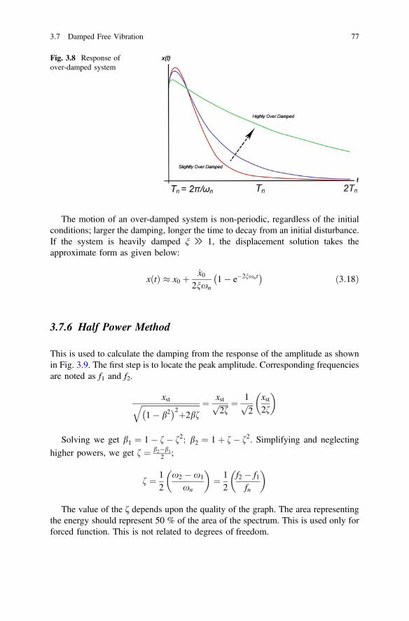
The motion of an over-damped system is non-periodic, regardless of the initialconditions; larger the damping, longer the time to decay from an initial disturbance.If the system is heavily damped ξ ≫ 1, the displacement solution takes theapproximate form as given below:
xðtÞ � x0 þ _x02nxn
1� e�2nxnt� � ð3:18Þ
3.7.6 Half Power Method
This is used to calculate the damping from the response of the amplitude as shownin Fig. 3.9. The first step is to locate the peak amplitude. Corresponding frequenciesare noted as f1 and f2.
xstffiffiffiffiffiffiffiffiffiffiffiffiffiffiffiffiffiffiffiffiffiffiffiffiffiffiffiffiffiffi1� b2� �2þ2bf
q ¼ xstffiffiffiffiffi2f
p ¼ 1ffiffiffi2
p xst2f
� �
Solving we get b1 ¼ 1� f� f2; b2 ¼ 1þ f� f2. Simplifying and neglectinghigher powers, we get f ¼ b2�b1
2 ;
f ¼ 12
x2 � x1
xn
� �¼ 1
2f2 � f1fn
� �
The value of the ζ depends upon the quality of the graph. The area representingthe energy should represent 50 % of the area of the spectrum. This is used only forforced function. This is not related to degrees of freedom.
Fig. 3.8 Response ofover-damped system
3.7 Damped Free Vibration 77
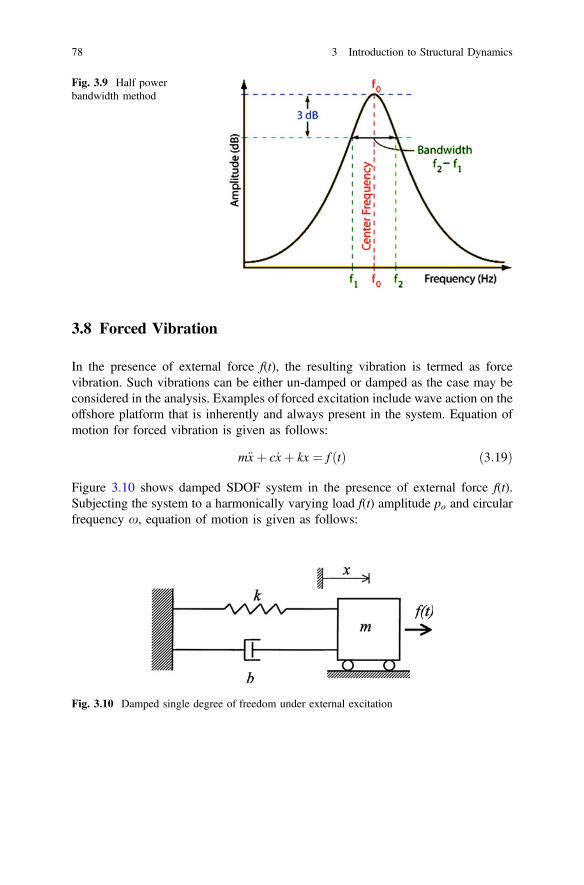
3.8 Forced Vibration
In the presence of external force f(t), the resulting vibration is termed as forcevibration. Such vibrations can be either un-damped or damped as the case may beconsidered in the analysis. Examples of forced excitation include wave action on theoffshore platform that is inherently and always present in the system. Equation ofmotion for forced vibration is given as follows:
m€xþ c _xþ kx ¼ f ðtÞ ð3:19Þ
Figure 3.10 shows damped SDOF system in the presence of external force f(t).Subjecting the system to a harmonically varying load f(t) amplitude po and circularfrequency x, equation of motion is given as follows:
Fig. 3.9 Half powerbandwidth method
Fig. 3.10 Damped single degree of freedom under external excitation
78 3 Introduction to Structural Dynamics
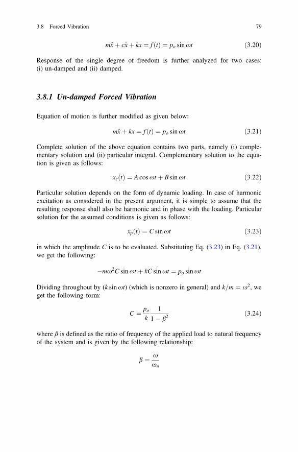
m€xþ c _xþ kx ¼ f ðtÞ ¼ po sinxt ð3:20Þ
Response of the single degree of freedom is further analyzed for two cases:(i) un-damped and (ii) damped.
3.8.1 Un-damped Forced Vibration
Equation of motion is further modified as given below:
m€xþ kx ¼ f ðtÞ ¼ po sinxt ð3:21Þ
Complete solution of the above equation contains two parts, namely (i) comple-mentary solution and (ii) particular integral. Complementary solution to the equa-tion is given as follows:
xcðtÞ ¼ A cosxt þ B sinxt ð3:22Þ
Particular solution depends on the form of dynamic loading. In case of harmonicexcitation as considered in the present argument, it is simple to assume that theresulting response shall also be harmonic and in phase with the loading. Particularsolution for the assumed conditions is given as follows:
xpðtÞ ¼ C sinxt ð3:23Þ
in which the amplitude C is to be evaluated. Substituting Eq. (3.23) in Eq. (3.21),we get the following:
�mx2C sinxt þ kC sinxt ¼ po sinxt
Dividing throughout by (k sinxt) (which is nonzero in general) and k=m ¼ x2, weget the following form:
C ¼ pok
1
1� b2ð3:24Þ
where β is defined as the ratio of frequency of the applied load to natural frequencyof the system and is given by the following relationship:
b ¼ xxn
3.8 Forced Vibration 79
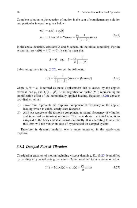
Complete solution to the equation of motion is the sum of complementary solutionand particular integral as given below:
xðtÞ ¼ xcðtÞ þ xpðtÞxðtÞ ¼ A cosxt þ B sinxt þ po
k1
½1� b2� sinxtð3:25Þ
In the above equation, constants A and B depend on the initial conditions. For thesystem at rest fxð0Þ ¼ _xð0Þ ¼ 0g, it can be seen that
A ¼ 0 and B ¼ pok
b
1� b2
Substituting these in Eq. (3.25), we get the following:
xðtÞ ¼ pok
1
½1� b2� ðsinxt � b sinxntÞ ð3:26Þ
where po=k ¼ xst is termed as static displacement that is caused by the appliedexternal load po and 1=ð1� b2Þ is the magnification factor (MF) representing theamplification effect of the harmonically applied loading. Equation (3.26) containstwo distinct terms:
(i) sinxt term represents the response component at frequency of the appliedloading which is called steady-state response
(ii) b sinxnt represents the response component at natural frequency of vibrationand is termed as transient response. This depends on the initial conditionsassigned to the body and shall vanish eventually. It is interesting to note thatthis term will not vanish in case of hypothetical un-damped system.
Therefore, in dynamic analysis, one is more interested in the steady-stateresponse.
3.8.2 Damped Forced Vibration
Considering equation of motion including viscous damping, Eq. (3.20) is modifiedby dividing it by m and noting that c=m ¼ 2nxn; modified form is given as below:
€xðtÞ þ 2nxn _xðtÞ þ x2xðtÞ ¼ p0msinxt ð3:27Þ
80 3 Introduction to Structural Dynamics
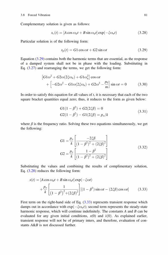
Complementary solution is given as follows:
xcðtÞ ¼ ½A cosxdt þ B sinxdt� expð�nxntÞ ð3:28Þ
Particular solution is of the following form:
xpðtÞ ¼ G1 cosxt þ G2 sinxt ð3:29Þ
Equation (3.29) contains both the harmonic terms that are essential, as the responseof a damped system shall not be in phase with the loading. Substituting inEq. (3.27) and rearranging the terms, we get the following form:
G1x2 þ G2x 2nxnð Þ þ G1x2n
cosxt
þ �G2x2 � G1x 2nxnð Þ þ G2x2 � p0m
h isinxt ¼ 0 ð3:30Þ
In order to satisfy this equation for all values of t, it is necessary that each of the twosquare bracket quantities equal zero; thus, it reduces to the form as given below:
G1ð1� b2Þ þ G2ð2nbÞ ¼ 0
G2ð1� b2Þ � G1ð2nbÞ ¼ po=kð3:31Þ
where β is the frequency ratio. Solving these two equations simultaneously, we getthe following:
G1 ¼ pok
�2nb
ð1� b2Þ2 þ ð2nbÞ2" #
G2 ¼ pok
1� b2
ð1� b2Þ2 þ ð2nbÞ2" # ð3:32Þ
Substituting the values and combining the results of complimentary solution,Eq. (3.28) reduces the following form:
xðtÞ ¼ ½A cosxdt þ B sinxdt� exp �nxtð Þ
þ pok
1
1� b2� �2þ 2nbð Þ2
" #½ð1� b2Þ sinxt � ð2nbÞ cosxt� ð3:33Þ
First term on the right-hand side of Eq. (3.33) represents transient response whichdamps out in accordance with expð�nxntÞ; second term represents the steady-stateharmonic response, which will continue indefinitely. The constants A and B can beevaluated for any given initial conditions, x(0) and _xð0Þ. As explained earlier,transient response will not be of primary inters, and therefore, evaluation of con-stants A&B is not discussed further.
3.8 Forced Vibration 81
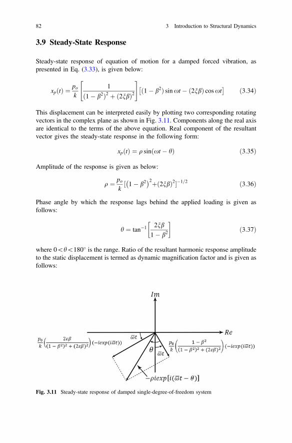
3.9 Steady-State Response
Steady-state response of equation of motion for a damped forced vibration, aspresented in Eq. (3.33), is given below:
xpðtÞ ¼ pok
1
ð1� b2Þ2 þ ð2nbÞ2" #
ð1� b2Þ sinxt � ð2nbÞ cosxt ð3:34Þ
This displacement can be interpreted easily by plotting two corresponding rotatingvectors in the complex plane as shown in Fig. 3.11. Components along the real axisare identical to the terms of the above equation. Real component of the resultantvector gives the steady-state response in the following form:
xpðtÞ ¼ q sinðxt � hÞ ð3:35Þ
Amplitude of the response is given as below:
q ¼ pok½ 1� b2� �2þ 2nbð Þ2��1=2 ð3:36Þ
Phase angle by which the response lags behind the applied loading is given asfollows:
h ¼ tan�1 2nb
1� b2
� �ð3:37Þ
where 0\h\180� is the range. Ratio of the resultant harmonic response amplitudeto the static displacement is termed as dynamic magnification factor and is given asfollows:
Fig. 3.11 Steady-state response of damped single-degree-of-freedom system
82 3 Introduction to Structural Dynamics
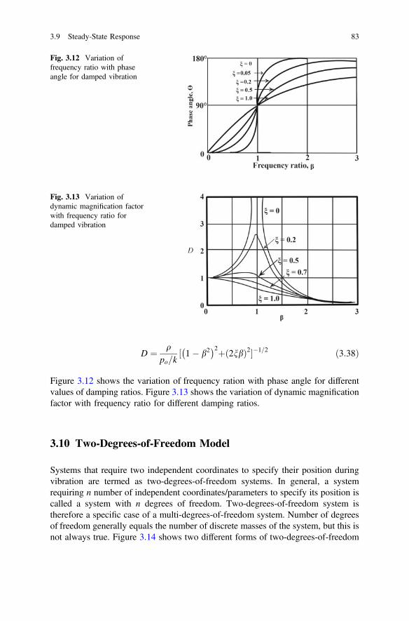
D ¼ qpo=k
½ 1� b2� �2þ 2nbð Þ2��1=2 ð3:38Þ
Figure 3.12 shows the variation of frequency ration with phase angle for differentvalues of damping ratios. Figure 3.13 shows the variation of dynamic magnificationfactor with frequency ratio for different damping ratios.
3.10 Two-Degrees-of-Freedom Model
Systems that require two independent coordinates to specify their position duringvibration are termed as two-degrees-of-freedom systems. In general, a systemrequiring n number of independent coordinates/parameters to specify its position iscalled a system with n degrees of freedom. Two-degrees-of-freedom system istherefore a specific case of a multi-degrees-of-freedom system. Number of degreesof freedom generally equals the number of discrete masses of the system, but this isnot always true. Figure 3.14 shows two different forms of two-degrees-of-freedom
Fig. 3.12 Variation offrequency ratio with phaseangle for damped vibration
Fig. 3.13 Variation ofdynamic magnification factorwith frequency ratio fordamped vibration
3.9 Steady-State Response 83
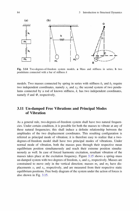
models. Two masses connected by spring in series with stiffness k1 and k2 requiretwo independent coordinates, namely x1 and x2; the second system of two pendu-lums connected by a rod of known stiffness, k, has two independent coordinates,namely θ and Φ, respectively.
3.11 Un-damped Free Vibrations and Principal Modesof Vibration
As a general rule, two-degrees-of-freedom system shall have two natural frequen-cies. Under certain condition, it is possible for both the masses to vibrate at any ofthese natural frequencies; this shall induce a definite relationship between theamplitudes of the two displacement coordinates. This resulting configuration isreferred as principal mode of vibration; it is therefore easy to realize that a two-degrees-of-freedom model shall have two principal modes of vibrations. Undernormal mode of vibration, both the masses pass through their respective meanequilibrium position simultaneously and reach their extreme position simulta-neously as well. In case of forced harmonic excitation, resultant vibration of themasses takes place at the excitation frequency. Figure 3.15 shows a spring–massun-damped system with two degrees of freedom, x1 and x2, respectively. Masses areconstrained to move only in the vertical direction; masses m1 and m2 have dis-placements x1 and x1, respectively, and are measured from their respective staticequilibrium positions. Free body diagram of the system under the action of forces isalso shown in Fig. 3.15.
(a) (b)
m1
m2m1
m2
k1
k2
k
O
C
B
φ φθ
θ
Fig. 3.14 Two-degrees-of-freedom system models. a Mass and stiffness in series; b twopendulums connected with a bar of stiffness k
84 3 Introduction to Structural Dynamics
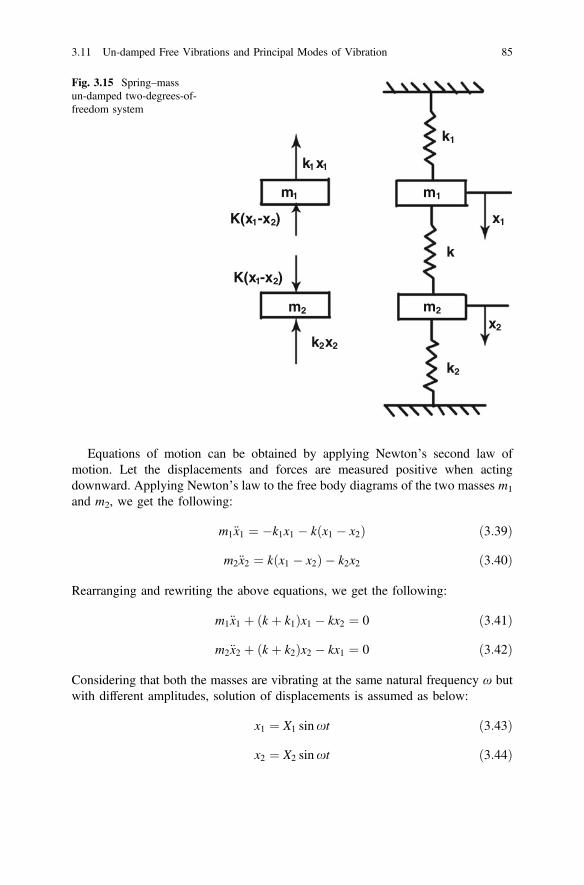
Equations of motion can be obtained by applying Newton’s second law ofmotion. Let the displacements and forces are measured positive when actingdownward. Applying Newton’s law to the free body diagrams of the two masses m1
and m2, we get the following:
m1€x1 ¼ �k1x1 � k x1 � x2ð Þ ð3:39Þ
m2€x2 ¼ k x1 � x2ð Þ � k2x2 ð3:40Þ
Rearranging and rewriting the above equations, we get the following:
m1€x1 þ k þ k1ð Þx1 � kx2 ¼ 0 ð3:41Þ
m2€x2 þ k þ k2ð Þx2 � kx1 ¼ 0 ð3:42Þ
Considering that both the masses are vibrating at the same natural frequency ω butwith different amplitudes, solution of displacements is assumed as below:
x1 ¼ X1 sinxt ð3:43Þ
x2 ¼ X2 sinxt ð3:44Þ
m1 m1
m2m2
k1
k2
k
x1
x2
k1x1
k2x2
K(x1-x2)
K(x1-x2)
Fig. 3.15 Spring–massun-damped two-degrees-of-freedom system
3.11 Un-damped Free Vibrations and Principal Modes of Vibration 85
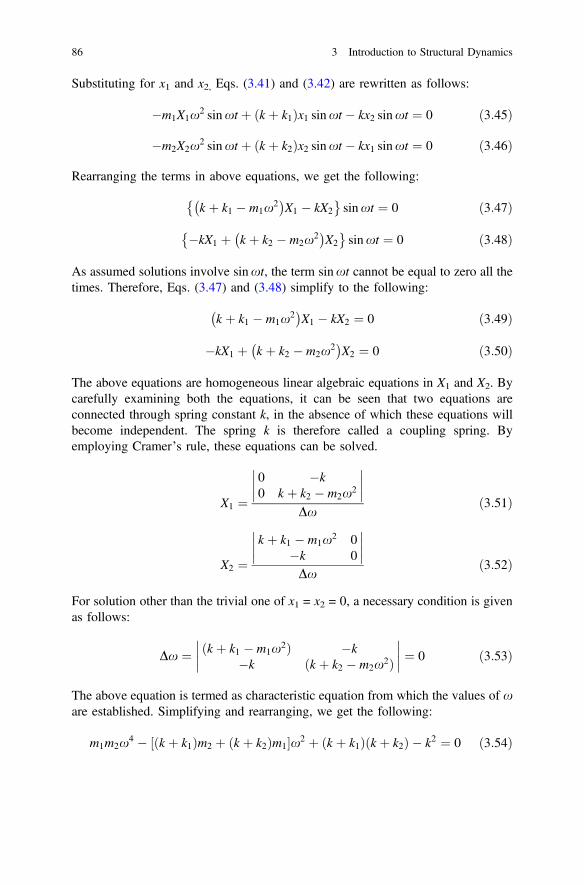
Substituting for x1 and x2, Eqs. (3.41) and (3.42) are rewritten as follows:
�m1X1x2 sinxt þ k þ k1ð Þx1 sinxt � kx2 sinxt ¼ 0 ð3:45Þ
�m2X2x2 sinxt þ k þ k2ð Þx2 sinxt � kx1 sinxt ¼ 0 ð3:46Þ
Rearranging the terms in above equations, we get the following:
k þ k1 � m1x2� �X1 � kX2
� �sinxt ¼ 0 ð3:47Þ
�kX1 þ k þ k2 � m2x2� �X2
� �sinxt ¼ 0 ð3:48Þ
As assumed solutions involve sinxt, the term sinxt cannot be equal to zero all thetimes. Therefore, Eqs. (3.47) and (3.48) simplify to the following:
k þ k1 � m1x2� �X1 � kX2 ¼ 0 ð3:49Þ
�kX1 þ k þ k2 � m2x2� �X2 ¼ 0 ð3:50Þ
The above equations are homogeneous linear algebraic equations in X1 and X2. Bycarefully examining both the equations, it can be seen that two equations areconnected through spring constant k, in the absence of which these equations willbecome independent. The spring k is therefore called a coupling spring. Byemploying Cramer’s rule, these equations can be solved.
X1 ¼0 �k0 k þ k2 � m2x2
Dxð3:51Þ
X2 ¼k þ k1 � m1x2 0
�k 0
Dxð3:52Þ
For solution other than the trivial one of x1 = x2 = 0, a necessary condition is givenas follows:
Dx ¼ ðk þ k1 � m1x2Þ �k�k ðk þ k2 � m2x2Þ
¼ 0 ð3:53Þ
The above equation is termed as characteristic equation from which the values of xare established. Simplifying and rearranging, we get the following:
m1m2x4 � k þ k1ð Þm2 þ k þ k2ð Þm1½ �x2 þ k þ k1ð Þ k þ k2ð Þ � k2 ¼ 0 ð3:54Þ
86 3 Introduction to Structural Dynamics
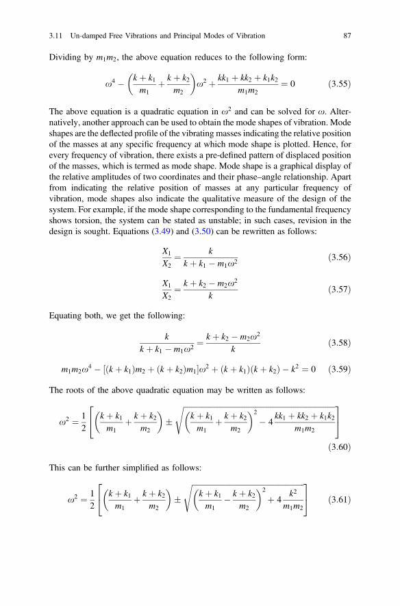
Dividing by m1m2, the above equation reduces to the following form:
x4 � k þ k1m1
þ k þ k2m2
� �x2 þ kk1 þ kk2 þ k1k2
m1m2¼ 0 ð3:55Þ
The above equation is a quadratic equation in x2 and can be solved for x. Alter-natively, another approach can be used to obtain the mode shapes of vibration. Modeshapes are the deflected profile of the vibrating masses indicating the relative positionof the masses at any specific frequency at which mode shape is plotted. Hence, forevery frequency of vibration, there exists a pre-defined pattern of displaced positionof the masses, which is termed as mode shape. Mode shape is a graphical display ofthe relative amplitudes of two coordinates and their phase–angle relationship. Apartfrom indicating the relative position of masses at any particular frequency ofvibration, mode shapes also indicate the qualitative measure of the design of thesystem. For example, if the mode shape corresponding to the fundamental frequencyshows torsion, the system can be stated as unstable; in such cases, revision in thedesign is sought. Equations (3.49) and (3.50) can be rewritten as follows:
X1
X2¼ k
k þ k1 � m1x2 ð3:56Þ
X1
X2¼ k þ k2 � m2x2
kð3:57Þ
Equating both, we get the following:
kk þ k1 � m1x2 ¼
k þ k2 � m2x2
kð3:58Þ
m1m2x4 � k þ k1ð Þm2 þ k þ k2ð Þm1½ �x2 þ k þ k1ð Þ k þ k2ð Þ � k2 ¼ 0 ð3:59Þ
The roots of the above quadratic equation may be written as follows:
x2 ¼ 12
k þ k1m1
þ k þ k2m2
� ��
ffiffiffiffiffiffiffiffiffiffiffiffiffiffiffiffiffiffiffiffiffiffiffiffiffiffiffiffiffiffiffiffiffiffiffiffiffiffiffiffiffiffiffiffiffiffiffiffiffiffiffiffiffiffiffiffiffiffiffiffiffiffiffiffiffiffiffiffiffiffiffiffiffiffiffiffiffiffiffiffik þ k1m1
þ k þ k2m2
� �2
� 4kk1 þ kk2 þ k1k2
m1m2
s24
35
ð3:60Þ
This can be further simplified as follows:
x2 ¼ 12
k þ k1m1
þ k þ k2m2
� ��
ffiffiffiffiffiffiffiffiffiffiffiffiffiffiffiffiffiffiffiffiffiffiffiffiffiffiffiffiffiffiffiffiffiffiffiffiffiffiffiffiffiffiffiffiffiffiffiffiffiffiffiffiffiffiffiffiffiffiffik þ k1m1
� k þ k2m2
� �2
þ 4k2
m1m2
s24
35 ð3:61Þ
3.11 Un-damped Free Vibrations and Principal Modes of Vibration 87
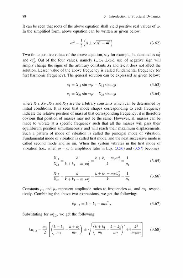
It can be seen that roots of the above equation shall yield positive real values of ω.In the simplified form, above equation can be written as given below:
x2 ¼ 12
A�ffiffiffiffiffiffiffiffiffiffiffiffiffiffiffiffiA2 � 4B
p� �ð3:62Þ
Two finite positive values of the above equation, say for example, be denoted as x21
and x22. Out of the four values, namely (�x1;�x2), use of negative sign will
simply change the signs of the arbitrary constants X1 and X2; it does not affect thesolution. Lesser value of the above frequency is called fundamental frequency (orfirst harmonic frequency). The general solution can be expressed as given below:
x1 ¼ X11 sinx1t þ X12 sinx2t ð3:63Þ
x2 ¼ X21 sinx1t þ X22 sinx2t ð3:64Þ
where X11;X12;X21 and X22 are the arbitrary constants which can be determined byinitial conditions. It is seen that mode shapes corresponding to each frequencyindicate the relative position of mass at that corresponding frequency; it is thereforeobvious that position of masses may not be the same. However, all masses can bemade to vibrate at a specific frequency such that all the masses will pass theirequilibrium position simultaneously and will reach their maximum displacements.Such a pattern of mode of vibration is called the principal mode of vibration.Fundamental mode of vibration is called first mode, and the next successive mode iscalled second mode and so on. When the system vibrates in the first mode ofvibration (i.e., when x ¼ x1), amplitude ratio in Eqs. (3.56) and (3.57) becomes
X11
X21¼ k
k þ k1 � m1x21¼ k þ k2 � m2x2
1
k¼ 1
l1ð3:65Þ
X12
X22¼ k
k þ k1 � m1x22¼ k þ k2 � m2x2
2
k¼ 1
l2ð3:66Þ
Constants l1 and l2 represent amplitude ratios to frequencies x1 and x2, respec-tively. Combining the above two expressions, we get the following:
kl1;2 ¼ k þ k1 � mx21;2 ð3:67Þ
Substituting for x21;2; we get the following:
kl1;2 ¼m1
2k þ k1m1
� k þ k2m2
� ��
ffiffiffiffiffiffiffiffiffiffiffiffiffiffiffiffiffiffiffiffiffiffiffiffiffiffiffiffiffiffiffiffiffiffiffiffiffiffiffiffiffiffiffiffiffiffiffiffiffiffiffiffiffiffiffiffiffik þ k1m1
� k þ k2m2
� �2
þ4k2
m1m2
s24
35 ð3:68Þ
88 3 Introduction to Structural Dynamics
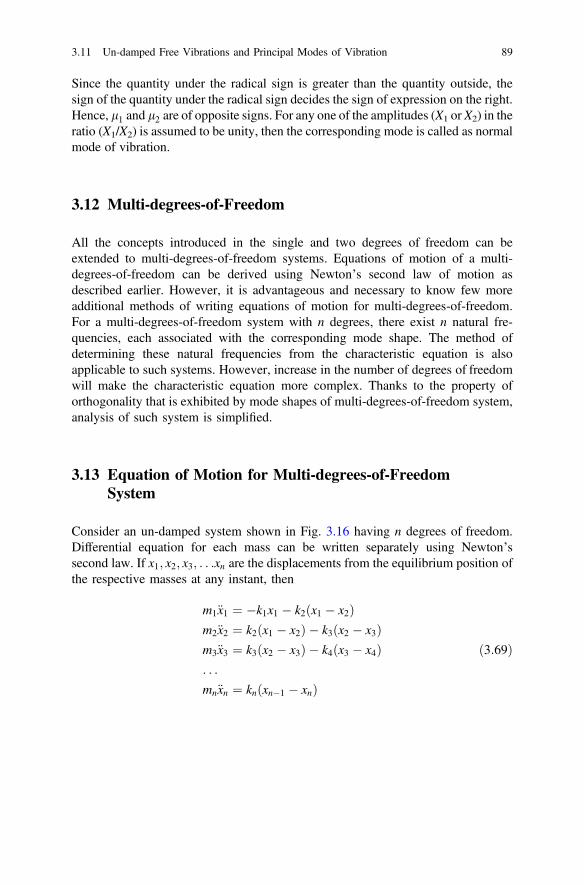
Since the quantity under the radical sign is greater than the quantity outside, thesign of the quantity under the radical sign decides the sign of expression on the right.Hence, l1 and l2 are of opposite signs. For any one of the amplitudes (X1 or X2) in theratio (X1/X2) is assumed to be unity, then the corresponding mode is called as normalmode of vibration.
3.12 Multi-degrees-of-Freedom
All the concepts introduced in the single and two degrees of freedom can beextended to multi-degrees-of-freedom systems. Equations of motion of a multi-degrees-of-freedom can be derived using Newton’s second law of motion asdescribed earlier. However, it is advantageous and necessary to know few moreadditional methods of writing equations of motion for multi-degrees-of-freedom.For a multi-degrees-of-freedom system with n degrees, there exist n natural fre-quencies, each associated with the corresponding mode shape. The method ofdetermining these natural frequencies from the characteristic equation is alsoapplicable to such systems. However, increase in the number of degrees of freedomwill make the characteristic equation more complex. Thanks to the property oforthogonality that is exhibited by mode shapes of multi-degrees-of-freedom system,analysis of such system is simplified.
3.13 Equation of Motion for Multi-degrees-of-FreedomSystem
Consider an un-damped system shown in Fig. 3.16 having n degrees of freedom.Differential equation for each mass can be written separately using Newton’ssecond law. If x1; x2; x3; . . .xn are the displacements from the equilibrium position ofthe respective masses at any instant, then
m1€x1 ¼ �k1x1 � k2ðx1 � x2Þm2€x2 ¼ k2 x1 � x2ð Þ � k3ðx2 � x3Þm3€x3 ¼ k3 x2 � x3ð Þ � k4 x3 � x4ð Þ. . .
mn€xn ¼ kn xn�1 � xnð Þ
ð3:69Þ
3.11 Un-damped Free Vibrations and Principal Modes of Vibration 89
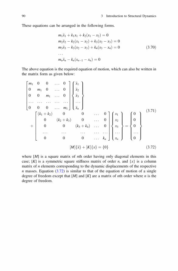
These equations can be arranged in the following forms.
m1€x1 þ k1x1 þ k2 x1 � x2ð Þ ¼ 0
m2€x2 � k2 x1 � x2ð Þ þ k3 x2 � x3ð Þ ¼ 0
m3€x3 � k3 x2 � x3ð Þ þ k4 x3 � x4ð Þ ¼ 0
. . .
mn€xn � kn xn�1 � xnð Þ ¼ 0
ð3:70Þ
The above equation is the required equation of motion, which can also be written inthe matrix form as given below:
m1 0 0 . . . 0
0 m1 0 . . . 0
0 0 m1 . . . 0
. . . . . . . . . . . . . . .
0 0 0 . . . m1
26666664
37777775
€x1€x2€x3. . .
€xn
8>>>>>><>>>>>>:
9>>>>>>=>>>>>>;
þ
ðk1 þ k2Þ 0 0 . . . 0
0 ðk2 þ k3Þ 0 . . . 0
0 0 ðk3 þ k4Þ . . . 0
. . . . . . . . . . . . . . .
0 0 0 . . . kn
26666664
37777775
x1x2x3. . .
xn
8>>>>>><>>>>>>:
9>>>>>>=>>>>>>;
¼
0
0
0
. . .
0
8>>>>>><>>>>>>:
9>>>>>>=>>>>>>;
ð3:71Þ
½M�f€xg þ ½K�fxg ¼ f0g ð3:72Þ
where [M] is a square matrix of nth order having only diagonal elements in thiscase; [K] is a symmetric square stiffness matrix of order n, and {x} is a columnmatrix of n elements corresponding to the dynamic displacements of the respectiven masses. Equation (3.72) is similar to that of the equation of motion of a singledegree of freedom except that [M] and [K] are a matrix of nth order where n is thedegree of freedom.
90 3 Introduction to Structural Dynamics
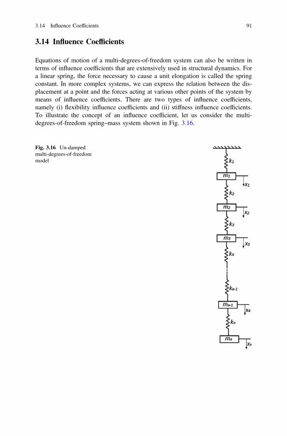
3.14 Influence Coefficients
Equations of motion of a multi-degrees-of-freedom system can also be written interms of influence coefficients that are extensively used in structural dynamics. Fora linear spring, the force necessary to cause a unit elongation is called the springconstant. In more complex systems, we can express the relation between the dis-placement at a point and the forces acting at various other points of the system bymeans of influence coefficients. There are two types of influence coefficients,namely (i) flexibility influence coefficients and (ii) stiffness influence coefficients.To illustrate the concept of an influence coefficient, let us consider the multi-degrees-of-freedom spring–mass system shown in Fig. 3.16.
Fig. 3.16 Un-dampedmulti-degrees-of-freedommodel
3.14 Influence Coefficients 91
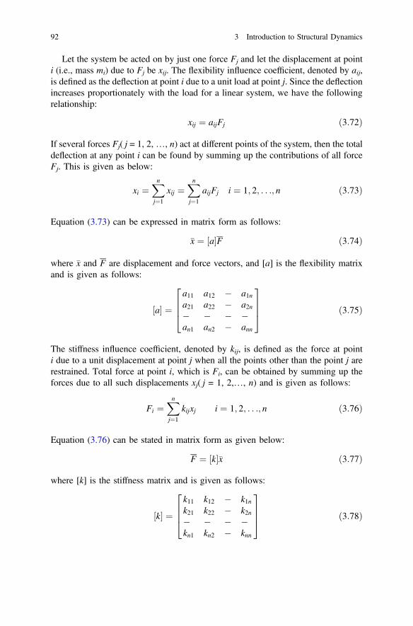
Let the system be acted on by just one force Fj and let the displacement at pointi (i.e., mass mi) due to Fj be xij. The flexibility influence coefficient, denoted by aij,is defined as the deflection at point i due to a unit load at point j. Since the deflectionincreases proportionately with the load for a linear system, we have the followingrelationship:
xij ¼ aijFj ð3:72Þ
If several forces Fj( j = 1, 2,…, n) act at different points of the system, then the totaldeflection at any point i can be found by summing up the contributions of all forceFj. This is given as below:
xi ¼Xnj¼1
xij ¼Xnj¼1
aijFj i ¼ 1; 2; . . .; n ð3:73Þ
Equation (3.73) can be expressed in matrix form as follows:
�x ¼ ½a�F ð3:74Þ
where �x and F are displacement and force vectors, and [a] is the flexibility matrixand is given as follows:
½a� ¼a11 a12 � a1na21 a22 � a2n� � � �an1 an2 � ann
2664
3775 ð3:75Þ
The stiffness influence coefficient, denoted by kij, is defined as the force at pointi due to a unit displacement at point j when all the points other than the point j arerestrained. Total force at point i, which is Fi, can be obtained by summing up theforces due to all such displacements xj( j = 1, 2,…, n) and is given as follows:
Fi ¼Xnj¼1
kijxj i ¼ 1; 2; . . .; n ð3:76Þ
Equation (3.76) can be stated in matrix form as given below:
F ¼ ½k��x ð3:77Þ
where [k] is the stiffness matrix and is given as follows:
½k� ¼k11 k12 � k1nk21 k22 � k2n� � � �kn1 kn2 � knn
2664
3775 ð3:78Þ
92 3 Introduction to Structural Dynamics
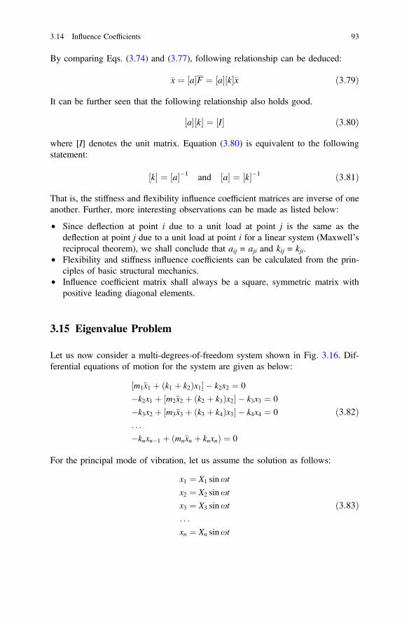
By comparing Eqs. (3.74) and (3.77), following relationship can be deduced:
�x ¼ ½a�F ¼ ½a�½k��x ð3:79Þ
It can be further seen that the following relationship also holds good.
½a�½k� ¼ ½I� ð3:80Þ
where [I] denotes the unit matrix. Equation (3.80) is equivalent to the followingstatement:
½k� ¼ ½a��1 and ½a� ¼ ½k��1 ð3:81Þ
That is, the stiffness and flexibility influence coefficient matrices are inverse of oneanother. Further, more interesting observations can be made as listed below:
• Since deflection at point i due to a unit load at point j is the same as thedeflection at point j due to a unit load at point i for a linear system (Maxwell’sreciprocal theorem), we shall conclude that aij = aji and kij = kji.
• Flexibility and stiffness influence coefficients can be calculated from the prin-ciples of basic structural mechanics.
• Influence coefficient matrix shall always be a square, symmetric matrix withpositive leading diagonal elements.
3.15 Eigenvalue Problem
Let us now consider a multi-degrees-of-freedom system shown in Fig. 3.16. Dif-ferential equations of motion for the system are given as below:
½m1€x1 þ k1 þ k2ð Þx1� � k2x2 ¼ 0
�k2x1 þ ½m2€x2 þ k2 þ k3ð Þx2� � k3x3 ¼ 0
�k3x2 þ ½m3€x3 þ k3 þ k4ð Þx3� � k4x4 ¼ 0
. . .
�knxn�1 þ ðmn€xn þ knxnÞ ¼ 0
ð3:82Þ
For the principal mode of vibration, let us assume the solution as follows:
x1 ¼ X1 sinxt
x2 ¼ X2 sinxt
x3 ¼ X3 sinxt
. . .
xn ¼ Xn sinxt
ð3:83Þ
3.14 Influence Coefficients 93
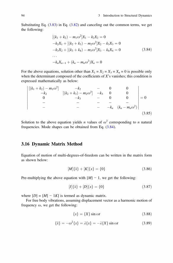
Substituting Eq. (3.83) in Eq. (3.82) and canceling out the common terms, we getthe following:
½ k1 þ k2ð Þ � m1x2�X1 � k2X2 ¼ 0
�k2X1 þ ½ k2 þ k3ð Þ � m2x2�X2 � k3X3 ¼ 0
�k3X2 þ ½ k3 þ k4ð Þ � m3x2�X3 � k4X4 ¼ 0
. . .
�knXn�1 þ ðkn � mnx2ÞXn ¼ 0
ð3:84Þ
For the above equations, solution other than X1 = X2 = X3 = Xn = 0 is possible onlywhen the determinant composed of the coefficients of X’s vanishes; this condition isexpressed mathematically as below:
½ðk1 þ k2Þ � m1x2� �k2 � 0 0�k2 ½ðk2 þ k3Þ � m2x2� �k3 0 00 �k3 � 0 0� � � � �� � � �kn ðkn � mnx2Þ
¼ 0
ð3:85Þ
Solution to the above equation yields n values of ω2 corresponding to n naturalfrequencies. Mode shapes can be obtained from Eq. (3.84).
3.16 Dynamic Matrix Method
Equation of motion of multi-degrees-of-freedom can be written in the matrix formas shown below:
½M�f€xg þ ½K�fxg ¼ f0g ð3:86Þ
Pre-multiplying the above equation with [M] − 1, we get the following:
½I�f€xg þ ½D�fxg ¼ f0g ð3:87Þ
where [D] = [M] − 1K] is termed as dynamic matrix.For free body vibrations, assuming displacement vector as a harmonic motion of
frequency ω, we get the following:
fxg ¼ fXg sinxt ð3:88Þ
f€xg ¼ �x2fxg ¼ kfxg ¼ �kfXg sinxt ð3:89Þ
94 3 Introduction to Structural Dynamics
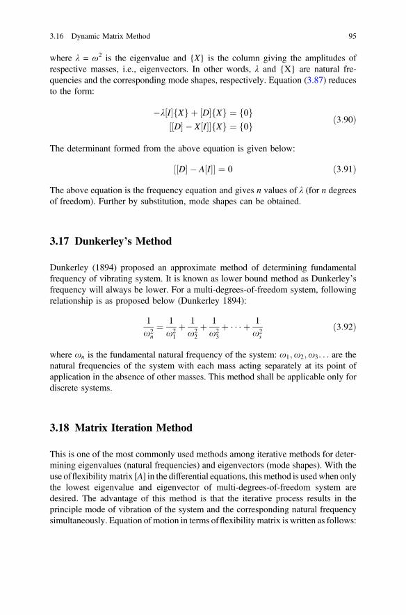
where λ = ω2 is the eigenvalue and {X} is the column giving the amplitudes ofrespective masses, i.e., eigenvectors. In other words, λ and {X} are natural fre-quencies and the corresponding mode shapes, respectively. Equation (3.87) reducesto the form:
�k½I�fXg þ ½D�fXg ¼ f0g½½D� � X½I��fXg ¼ f0g ð3:90Þ
The determinant formed from the above equation is given below:
½½D� � A½I�� ¼ 0 ð3:91Þ
The above equation is the frequency equation and gives n values of λ (for n degreesof freedom). Further by substitution, mode shapes can be obtained.
3.17 Dunkerley’s Method
Dunkerley (1894) proposed an approximate method of determining fundamentalfrequency of vibrating system. It is known as lower bound method as Dunkerley’sfrequency will always be lower. For a multi-degrees-of-freedom system, followingrelationship is as proposed below (Dunkerley 1894):
1x2
n¼ 1
x21þ 1x2
2þ 1x2
3þ � � � þ 1
x2s
ð3:92Þ
where xn is the fundamental natural frequency of the system: x1;x2;x3. . . are thenatural frequencies of the system with each mass acting separately at its point ofapplication in the absence of other masses. This method shall be applicable only fordiscrete systems.
3.18 Matrix Iteration Method
This is one of the most commonly used methods among iterative methods for deter-mining eigenvalues (natural frequencies) and eigenvectors (mode shapes). With theuse offlexibilitymatrix [A] in the differential equations, thismethod is usedwhen onlythe lowest eigenvalue and eigenvector of multi-degrees-of-freedom system aredesired. The advantage of this method is that the iterative process results in theprinciple mode of vibration of the system and the corresponding natural frequencysimultaneously. Equation of motion in terms offlexibility matrix is written as follows:
3.16 Dynamic Matrix Method 95
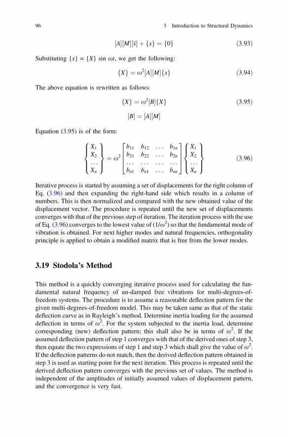
½A�½M�½€x� þ fxg ¼ f0g ð3:93Þ
Substituting {x} = {X} sin ωt, we get the following:
fXg ¼ x2½A�½M�fxg ð3:94Þ
The above equation is rewritten as follows:
fXg ¼ x2½B�fXg ð3:95Þ
½B� ¼ ½A�½M�
Equation (3.95) is of the form:
X1
X2
. . .Xn
8>><>>:
9>>=>>; ¼ x2
b11 b12 . . . b1nb21 b22 . . . b2n. . . . . . . . . . . .bn1 bn1 . . . bnn
2664
3775
X1
X2
. . .Xn
8>><>>:
9>>=>>; ð3:96Þ
Iterative process is started by assuming a set of displacements for the right column ofEq. (3.96) and then expanding the right-hand side which results in a column ofnumbers. This is then normalized and compared with the new obtained value of thedisplacement vector. The procedure is repeated until the new set of displacementsconverges with that of the previous step of iteration. The iteration process with the useof Eq. (3.96) converges to the lowest value of (1/ω2) so that the fundamental mode ofvibration is obtained. For next higher modes and natural frequencies, orthogonalityprinciple is applied to obtain a modified matrix that is free from the lower modes.
3.19 Stodola’s Method
This method is a quickly converging iterative process used for calculating the fun-damental natural frequency of un-damped free vibrations for multi-degrees-of-freedom systems. The procedure is to assume a reasonable deflection pattern for thegiven multi-degrees-of-freedom model. This may be taken same as that of the staticdeflection curve as in Rayleigh’s method. Determine inertia loading for the assumeddeflection in terms of ω2. For the system subjected to the inertia load, determinecorresponding (new) deflection pattern; this shall also be in terms of ω2. If theassumed deflection pattern of step 1 converges with that of the derived ones of step 3,then equate the two expressions of step 1 and step 3 which shall give the value of ω2.If the deflection patterns do not match, then the derived deflection pattern obtained instep 3 is used as starting point for the next iteration. This process is repeated until thederived deflection pattern converges with the previous set of values. The method isindependent of the amplitudes of initially assumed values of displacement pattern,and the convergence is very fast.
96 3 Introduction to Structural Dynamics
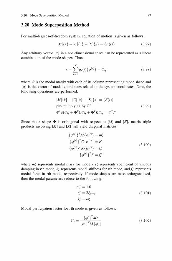
3.20 Mode Superposition Method
For multi-degrees-of-freedom system, equation of motion is given as follows:
½M�f€xg þ ½C�f _xg þ ½K�fxg ¼ fFðtÞg ð3:97Þ
Any arbitrary vector {x} in a non-dimensional space can be represented as a linearcombination of the mode shapes. Thus,
x ¼XNr¼1
qrðtÞfuðrÞg ¼ Uq ð3:98Þ
where U is the modal matrix with each of its column representing mode shape and{q} is the vector of modal coordinates related to the system coordinates. Now, thefollowing operations are performed:
½M�f€xg þ ½C�f _xg þ ½K�fxg ¼ fFðtÞgpre-multiplying by UT
UTMU€qþ UTCU _qþ UTKUq ¼ UTF
ð3:99Þ
Since mode shape U is orthogonal with respect to [M] and [K], matrix tripleproducts involving [M] and [K] will yield diagonal matrices.
fuðrÞgTMfuðrÞg ¼ m�r
fuðrÞgTCfuðrÞg ¼ c�rfuðrÞgTKfuðrÞg ¼ k�r
fuðrÞgTF ¼ f �r
ð3:100Þ
where m�r represents modal mass for mode r; c�r represents coefficient of viscous
damping in rth mode, k�r represents modal stiffness for rth mode, and f �r representsmodal force in rth mode, respectively. If mode shapes are mass-orthogonalized,then the modal parameters reduce to the following:
m�r ¼ 1:0
c�r ¼ 2nrxr
k�r ¼ x2r
ð3:101Þ
Modal participation factor for rth mode is given as follows:
Cr ¼ furgTMr
furgTMfurg ð3:102Þ
3.20 Mode Superposition Method 97
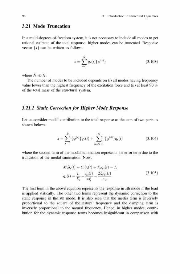
3.21 Mode Truncation
In a multi-degrees-of-freedom system, it is not necessary to include all modes to getrational estimate of the total response; higher modes can be truncated. Responsevector {x} can be written as follows:
x ¼XN̂r¼1
qrðtÞfuðrÞg ð3:103Þ
where N̂ N.The number of modes to be included depends on (i) all modes having frequency
value lower than the highest frequency of the excitation force and (ii) at least 90 %of the total mass of the structural system.
3.21.1 Static Correction for Higher Mode Response
Let us consider modal contribution to the total response as the sum of two parts asshown below:
x ¼X̂Nr¼1
fuðrÞgqrðtÞ þXN
S¼N̂þ1
fuðSÞgqsðtÞ ð3:104Þ
where the second term of the modal summation represents the error term due to thetruncation of the modal summation. Now,
Ms€qsðtÞ þ Cs _qsðtÞ þ KsqsðtÞ ¼ fs
qsðtÞ ¼ fsKs
� €qsðtÞx2
s� 2ns _qsðtÞ
xs
ð3:105Þ
The first term in the above equation represents the response in sth mode if the loadis applied statically. The other two terms represent the dynamic correction to thestatic response in the sth mode. It is also seen that the inertia term is inverselyproportional to the square of the natural frequency and the damping term isinversely proportional to the natural frequency. Hence, in higher modes, contri-bution for the dynamic response terms becomes insignificant in comparison with
98 3 Introduction to Structural Dynamics
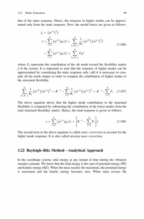
that of the static response. Hence, the response in higher modes can be approxi-mated only from the static response. Now, the modal forces are given as follows:
fs ¼ fuðsÞgT f
x ¼XN̂r¼1
fuðrÞgqrðtÞ þXN
S¼N̂þ1
1KS
fuðSÞgfuðsÞgT f
¼XN̂r¼1
fuðrÞgqrðtÞ þXN
S¼N̂þ1
FSf
ð3:106Þ
where FS represents the contribution of the sth mode toward the flexibility matrixf of the system. It is important to note that the response of higher modes can beapproximated by considering the static response only; still it is necessary to com-pute all the mode shapes in order to compute the contribution of higher modes tothe structural flexibility.
XNS¼N̂þ1
1KS
fuðSÞgfuðsÞgT ¼ K�1 �XN̂r¼1
1Kr
fuðrÞgfuðrÞgT ¼ K�1�XN̂r¼1
Fr ð3:107Þ
The above equation shows that the higher mode contribution to the structuralflexibility is computed by subtracting the contribution of the lower modes from thetotal structural flexibility matrix. Hence, the total response is given as follows:
x ¼XN̂r¼1
fuðrÞgqrðtÞ þ K�1 �XN̂r¼1
Fr
" #f ð3:108Þ
The second term in the above equation is called static correction to account for thehigher mode response. It is also called missing mass correction.
3.22 Rayleigh–Ritz Method—Analytical Approach
In the coordinate system, total energy at any instant of time during the vibrationremains constant. We know that the total energy is the sum of potential energy (PE)and kinetic energy (KE). When the mass reaches the maximum, the potential energyis maximum and the kinetic energy becomes zero. When mass crosses the
3.21 Mode Truncation 99
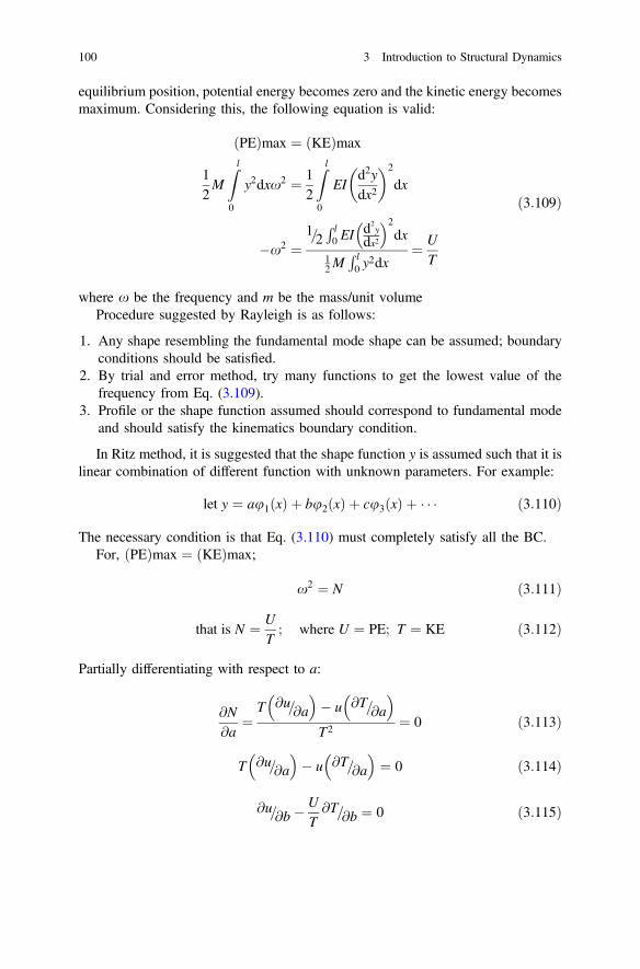
equilibrium position, potential energy becomes zero and the kinetic energy becomesmaximum. Considering this, the following equation is valid:
ðPEÞmax ¼ ðKEÞmax
12MZ l
0
y2dxx2 ¼ 12
Z l
0
EId2ydx2
� �2
dx
�x2 ¼1=2R l0 EI
d2y
dx2� �2
dx
12MR l0 y
2dx¼ U
T
ð3:109Þ
where x be the frequency and m be the mass/unit volumeProcedure suggested by Rayleigh is as follows:
1. Any shape resembling the fundamental mode shape can be assumed; boundaryconditions should be satisfied.
2. By trial and error method, try many functions to get the lowest value of thefrequency from Eq. (3.109).
3. Profile or the shape function assumed should correspond to fundamental modeand should satisfy the kinematics boundary condition.
In Ritz method, it is suggested that the shape function y is assumed such that it islinear combination of different function with unknown parameters. For example:
let y ¼ au1ðxÞ þ bu2ðxÞ þ cu3ðxÞ þ � � � ð3:110Þ
The necessary condition is that Eq. (3.110) must completely satisfy all the BC.For, ðPEÞmax ¼ ðKEÞmax;
x2 ¼ N ð3:111Þ
that is N ¼ UT; where U ¼ PE; T ¼ KE ð3:112Þ
Partially differentiating with respect to a:
@N@a
¼T @u=@a
� �� u @T=@a
� �T2 ¼ 0 ð3:113Þ
T @u=@a
� �� u @T=@a
� �¼ 0 ð3:114Þ
@u=@b�UT@T=@b ¼ 0 ð3:115Þ
100 3 Introduction to Structural Dynamics
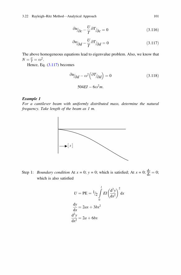
@u=@c�UT@T=@c ¼ 0 ð3:116Þ
@u=@d � UT@T=@d ¼ 0 ð3:117Þ
The above homogeneous equations lead to eigenvalue problem. Also, we know thatN ¼ U
T ¼ x2:
Hence, Eq. (3.117) becomes
@u=@d � x2 @T=@d
� �¼ 0 ð3:118Þ
504EI � 6x2m:
Example 1For a cantilever beam with uniformly distributed mass, determine the naturalfrequency. Take length of the beam as 1 m.
x[ ]
Step 1: Boundary condition At x = 0; y = 0; which is satisfied; At x = 0; dydx ¼ 0;
which is also satisfied
U ¼ PE ¼ 1=2
Z l
0
EId2ydx2
� �2
dx
dydx
¼ 2axþ 3bx2
d2ydx2
¼ 2aþ 6bx
3.22 Rayleigh–Ritz Method—Analytical Approach 101
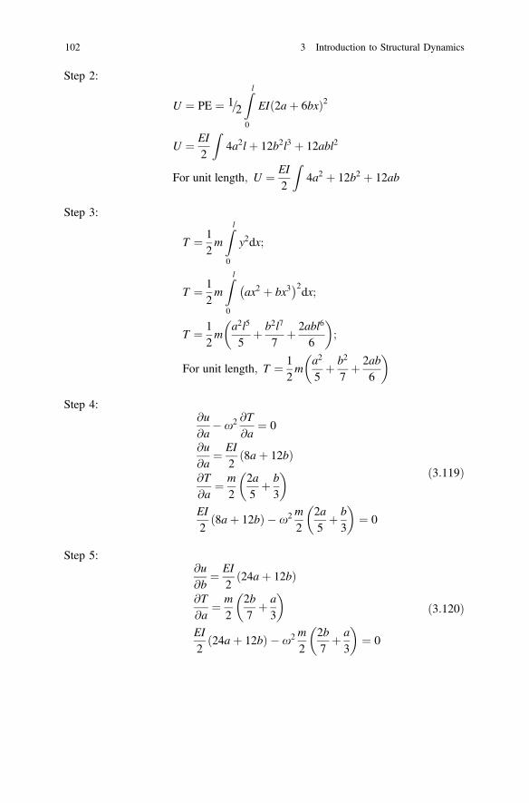
Step 2:
U ¼ PE ¼ 1=2
Z l
0
EI 2aþ 6bxð Þ2
U ¼ EI2
Z4a2lþ 12b2l3 þ 12abl2
For unit length; U ¼ EI2
Z4a2 þ 12b2 þ 12ab
Step 3:
T ¼ 12mZ l
0
y2dx;
T ¼ 12mZ l
0
ax2 þ bx3� �2
dx;
T ¼ 12m
a2l5
5þ b2l7
7þ 2abl6
6
� �;
For unit length; T ¼ 12m
a2
5þ b2
7þ 2ab
6
� �
Step 4:@u@a
� x2 @T@a
¼ 0
@u@a
¼ EI2
8aþ 12bð Þ@T@a
¼ m2
2a5þ b3
� �EI2
8aþ 12bð Þ � x2 m2
2a5þ b3
� �¼ 0
ð3:119Þ
Step 5:@u@b
¼ EI2
24aþ 12bð Þ@T@a
¼ m2
2b7þ a3
� �EI2
24aþ 12bð Þ � x2 m2
2b7þ a3
� �¼ 0
ð3:120Þ
102 3 Introduction to Structural Dynamics
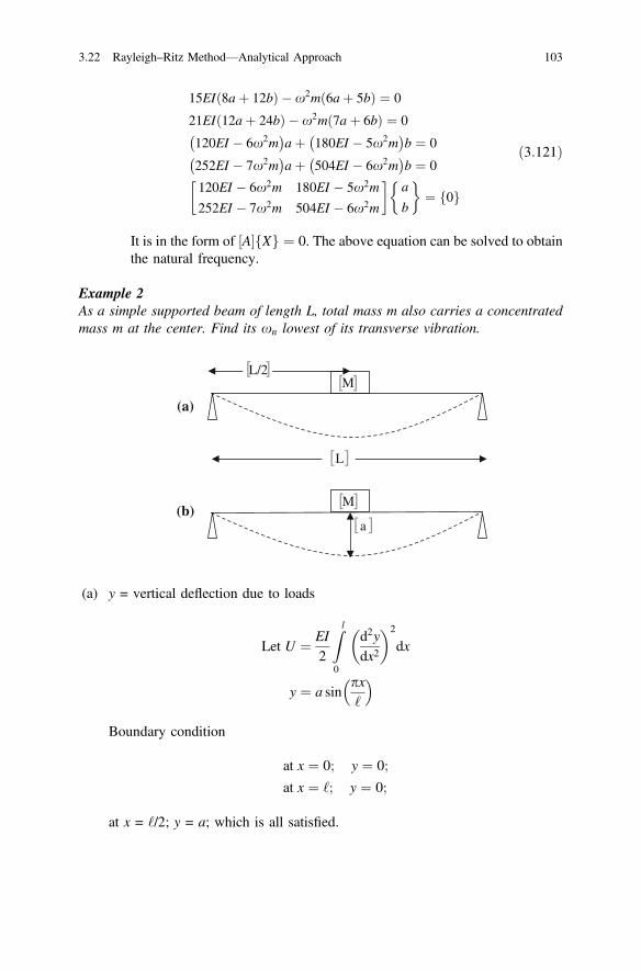
15EIð8aþ 12bÞ � x2mð6aþ 5bÞ ¼ 0
21EIð12aþ 24bÞ � x2m 7aþ 6bð Þ ¼ 0
120EI � 6x2m� �
aþ 180EI � 5x2m� �
b ¼ 0
252EI � 7x2m� �
aþ 504EI � 6x2m� �
b ¼ 0
120EI � 6x2m 180EI � 5x2m
252EI � 7x2m 504EI � 6x2m
� �a
b
� �¼ 0f g
ð3:121Þ
It is in the form of ½A�fXg ¼ 0. The above equation can be solved to obtainthe natural frequency.
Example 2As a simple supported beam of length L, total mass m also carries a concentratedmass m at the center. Find its xn lowest of its transverse vibration.
M
L
M
a
(a)
(b)
[ ]
[ ]
[ ]
L/2[ ]
[ ]
(a) y = vertical deflection due to loads
Let U ¼ EI2
Z l
0
d2ydx2
� �2
dx
y ¼ a sinpx‘
� �
Boundary condition
at x ¼ 0; y ¼ 0;
at x ¼ ‘; y ¼ 0;
at x = ‘/2; y = a; which is all satisfied.
3.22 Rayleigh–Ritz Method—Analytical Approach 103
dydx
¼ p‘
� �a cos
px‘
� �dydx
¼ � p‘
� �2a sin
px‘
� �
U ¼ EI2
Z l
0
p‘
� �2a sin
px‘
� �� �2dx
¼ EI2
Z l
0
p2
‘2
� �2
a2 sin2px‘
� �dx
letpx‘¼ h; cos 2h ¼ 1� 2 sin2 h;
sin2 h ¼ 12
1� cos 2h2
� �¼ 1
21� cos
2px‘
� �� �¼ 1
2
Z l
0
1� cos2px‘
� �� �dx
U ¼ EI2
p4
‘4
� �a2
12
Z l
0
1� cos2px‘
� �� �dx
U ¼ EI2
p‘
� �4‘a2
(a) Kinetic energy due to momentDeflection at middle = aLet the displacement x ¼ a cosxt; velocity =�ax sinxt; max velocity = j�axjKE due to concentrated mass M ¼ 1
2MV2 ¼ 12M a2x2ð Þ
(b) Due to mass of the beam m
T ¼ 12
m‘
� �Z‘0
y2dx ¼ 12
m‘
� �x2Z‘0
y2dx
¼ 12
m‘
� �x2 a2
2
� �Z‘0
1� cos2px‘
� �dx
T ¼ mx2a2
4
where m is the total mass of the entire beam.
104 3 Introduction to Structural Dynamics
Total KE ¼ 12Ma2x2 þ 1
4M x2a2� � ¼ 1
2x2a2 M þM
2
� �KEð Þmax ¼ PEð Þmax
x2 ¼EI ‘=2� �
p=‘� �4
M þ M4
� �
Comparison by Dunkerley’s Method
(a) Deflects due to central load, M
y11 ¼ 48EIM‘3
(b) Deflects due to total load,
y22 ¼ 48EIm‘3
1x2
� �¼ M‘3
48EIþ m‘3
p4EI
x2 ¼ EI p=‘� �4‘=2
1:013M þ M2
� �
Exercise
1. All bodies possess ___________ and _________________ which results invibration of the body.
2. At equilibrium, whole of elastic energy is converted into___________________ and the body continues to move in opposite directionbecause of it.
3. Whole of the kinetic energy is converted into___________________________ due to which the body again returns to theequilibrium position.
4. Any motion which repeats itself after an interval of time is called____________________.
5. A motion that repeats itself after equal interval of time is called__________________.
3.22 Rayleigh–Ritz Method—Analytical Approach 105

6. Number of cycles per unit time is called ________________.7. Maximum displacement of a vibrating body from the equilibrium position is
called ___________________________.8. When system vibrates without any external force, it is called
________________________.9. Natural frequency is expressed in ______________________ (units).
10. Minimum number of ________________________________ required tospecify the motion of system at any instant is known as___________________________.
11. Degree of freedom may vary between ______________________.12. ________________ beam is an example for infinite degrees of freedom.13. Motion of simple pendulum is an example for
_______________________________.14. Resistance offered to the motion of the vibrating body is called
___________________.15. When there is phase difference in the system, the vibrating motion can be
expressed as ____________________________________ (Hint: equation ofresponse).
16. When the frequency of external excitation is equal to natural frequency of thevibrating body, then the system is in ______________________ and amplitudeof vibration becomes extensively ____________________.
17. Mechanical system consists of _________________, __________________,and ______________________.
18. Continuous system is also called _____________________.19. In a vibrating system, there is an exchange of energy from
___________________.20. Energy is stored by mass in the form ________________ and spring in the
form of __________________.21. Sketch the basic vibratory system with SDOF.22. In the vibratory system, if the amount of external excitation is known in
magnitude, it is called ______________________________________.23. If system vibrates indefinitely and the amplitude decays because of
_________________ and vanishes continuously, such kind of vibration iscalled ________________________________.
24. _____________________________________ occurs as a result of interfer-ence between two waves of slightly different frequencies moving along thesame straight line in the same direction.
25. If springs with stiffness k1 and k2 are connected in parallel, their effectivestiffness is equal to ____________________.
26. ‘Mass develops an inertia force proportional to its acceleration and opposite indirection.’ This is stated by _____________________________.
106 3 Introduction to Structural Dynamics

27. The tension leg platform is heave restrained by _________________.28. Match the design wave height for various regions is tabulated below:
I. Bay of Bengal (a) 11 m for 1 yr and 24 m for 100 yrs
II. Gulf of Mexico (b) 6 m for 1 yr and 12 m for 100 yr
III. South China Sea (c) 5 m for 1 yr and 12 m for 100 yrs
IV. Arabian Sea (d) 14 m for 1 yr and 22 m for 100 yrs
V. Gulf of Thailand (e) 12 m for 1 yr and 24 m for 100 yrs
VI. Persian Gulf (f) 8 m for on 1 yr and 18 m for 100 yrs
VII. North Sea (g) 8 m for 1 yr and 18 m for 100 yrs
29. Growth of marine algae increases the ______________ and__________________which in turn increase the wave or current loading.
30. In P-M spectrum fetch and duration are considered _____________.31. Algebraic sum of wave and current loads is different from calculation of load
by adding the horizontal water particle velocity with the current velocity andcomputing the loads. This is because of____________________________________________.
32. Seismic loads are arising from derived type ___________.
Answers
1. Mass; restoring capacity (elasticity)2. Kinetic energy3. Elastic or strain energy4. Vibration or oscillation5. Periodic motion6. Frequency7. Amplitude8. Free vibration9. rad/s or hertz
10. Independent coordinates; degrees of freedom11. Zero to infinity12. Cantilever13. Simple harmonic motion14. Damping (friction)15. x = A sin (ωt + φ)16. Resonance; large
Exercise 107
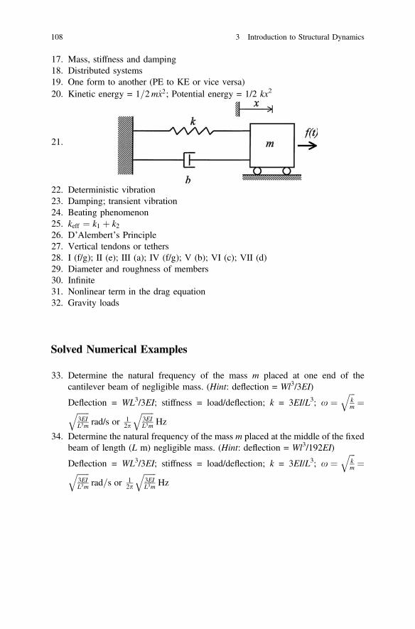
17. Mass, stiffness and damping18. Distributed systems19. One form to another (PE to KE or vice versa)20. Kinetic energy = 1=2m _x2; Potential energy = 1/2 kx2
21.
22. Deterministic vibration23. Damping; transient vibration24. Beating phenomenon25. keff ¼ k1 þ k226. D’Alembert’s Principle27. Vertical tendons or tethers28. I (f/g); II (e); III (a); IV (f/g); V (b); VI (c); VII (d)29. Diameter and roughness of members30. Infinite31. Nonlinear term in the drag equation32. Gravity loads
Solved Numerical Examples
33. Determine the natural frequency of the mass m placed at one end of thecantilever beam of negligible mass. (Hint: deflection = Wl3/3EI)
Deflection = WL3/3EI; stiffness = load/deflection; k = 3EI/L3; x ¼ffiffiffikm
q¼ffiffiffiffiffiffi
3EIL3m
qrad/s or 1
2p
ffiffiffiffiffiffi3EIL3m
qHz
34. Determine the natural frequency of the mass m placed at the middle of the fixedbeam of length (L m) negligible mass. (Hint: deflection = Wl3/192EI)
Deflection = WL3/3EI; stiffness = load/deflection; k = 3EI/L3; x ¼ffiffiffikm
q¼ffiffiffiffiffiffi
3EIL3m
qrad=s or 1
2p
ffiffiffiffiffiffi3EIL3m
qHz
108 3 Introduction to Structural Dynamics
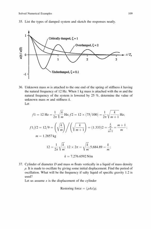
35. List the types of damped system and sketch the responses neatly.
36. Unknown mass m is attached to the one end of the spring of stiffness k havingthe natural frequency of 12 Hz. When 1 kg mass is attached with the m and thenatural frequency of the system is lowered by 25 %, determine the value ofunknown mass m and stiffness k.Let
f 1 ¼ 12 Hz ¼ 12p
ffiffiffiffikm
rHz; f 2 ¼ 12 75=100ð Þ ¼ 1
2p
ffiffiffiffiffiffiffiffiffiffiffiffik
mþ 1
rHz;
f 1=f 2 ¼ 12=9 ¼ffiffiffiffikm
r !, ffiffiffiffiffiffiffiffiffiffiffiffik
mþ 1
r !¼ 1:333ð Þ2 ¼
kmk
mþ1
¼ mþ 1m
;
m ¼ 1:2857 kg
12 ¼ 12p
ffiffiffiffikm
r; 12 2p ¼
ffiffiffiffikm
r; 5;684:89 ¼ k
m;
k ¼ 7;276:6592N/m
37. Cylinder of diameter D and mass m floats vertically in a liquid of mass densityρ. It is made to oscillate by giving some initial displacement. Find the period ofoscillation. What will be the frequency if salty liquid of specific gravity 1.2 isused?Let us assume x is the displacement of the cylinder
Restoring force ¼ ðqAxÞg;
Solved Numerical Examples 109
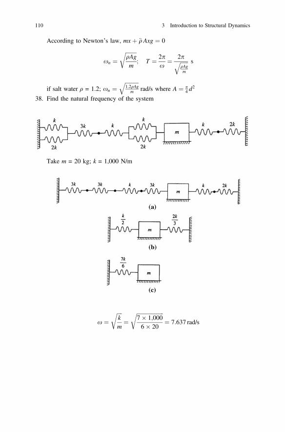
According to Newton’s law, mxþ €qAxg ¼ 0
xn ¼ffiffiffiffiffiffiffiffiqAgm
r; T ¼ 2p
x¼ 2pffiffiffiffiffiffi
qAgm
q s
if salt water ρ = 1.2; xn ¼ffiffiffiffiffiffiffiffiffiffi1:2qAg
m
qrad/s where A ¼ p
4 d2
38. Find the natural frequency of the system
Take m = 20 kg; k = 1,000 N/m
x ¼ffiffiffiffikm
r¼
ffiffiffiffiffiffiffiffiffiffiffiffiffiffiffiffiffiffiffiffi7 1;0006 20
r¼ 7:637 rad/s
110 3 Introduction to Structural Dynamics
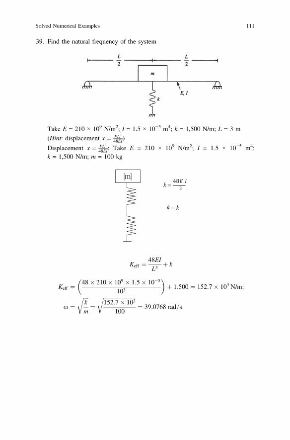
39. Find the natural frequency of the system
Take E = 210 × 109 N/m2; I = 1.5 × 10⁻⁵ m4; k = 1,500 N/m; L = 3 m(Hint: displacement x ¼ PL3
48EI)
Displacement x ¼ PL348EI; Take E = 210 × 109 N/m2; I = 1.5 × 10⁻⁵ m4;
k = 1,500 N/m; m = 100 kg
m[ ]
Keff ¼ 48EIL3
þ k
Keff ¼ 48 210 109 1:5 10�5
103
� �þ 1;500 ¼ 152:7 103 N/m;
x ¼ffiffiffiffikm
r¼
ffiffiffiffiffiffiffiffiffiffiffiffiffiffiffiffiffiffiffiffiffiffiffiffi152:7 103
100
r¼ 39:0768 rad=s
Solved Numerical Examples 111
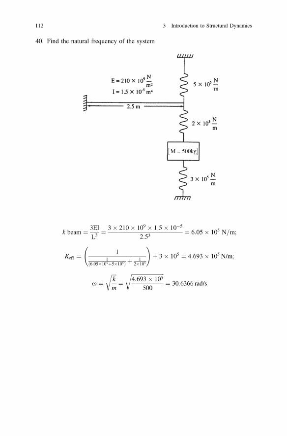
40. Find the natural frequency of the system
M = 500kg[ ]
k beam ¼ 3EIL3 ¼ 3 210 109 1:5 10�5
2:53¼ 6:05 105 N=m;
Keff ¼ 11
6:05105þ5105ð Þ þ 12105
!þ 3 105 ¼ 4:693 105 N/m;
x ¼ffiffiffiffikm
r¼
ffiffiffiffiffiffiffiffiffiffiffiffiffiffiffiffiffiffiffiffiffiffiffiffi4:693 105
500
r¼ 30:6366 rad/s
112 3 Introduction to Structural Dynamics
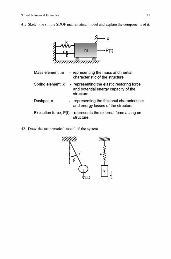
41. Sketch the simple SDOF mathematical model and explain the components of it.
42. Draw the mathematical model of the system
Solved Numerical Examples 113
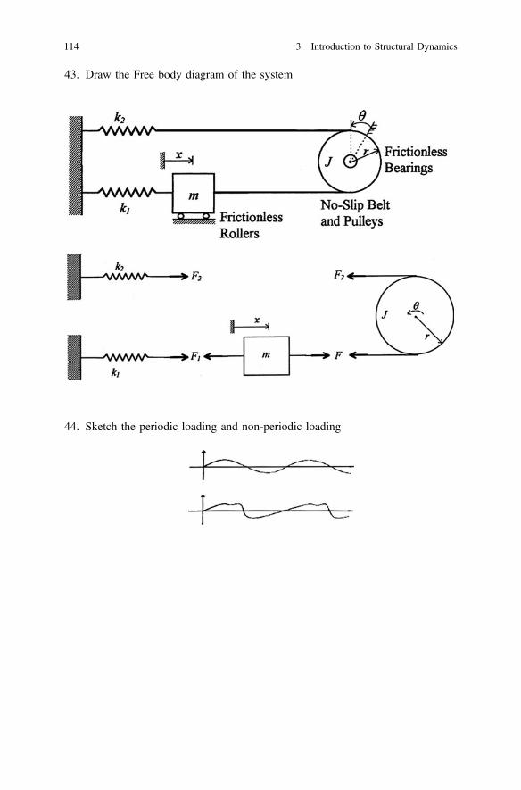
43. Draw the Free body diagram of the system
44. Sketch the periodic loading and non-periodic loading
114 3 Introduction to Structural Dynamics
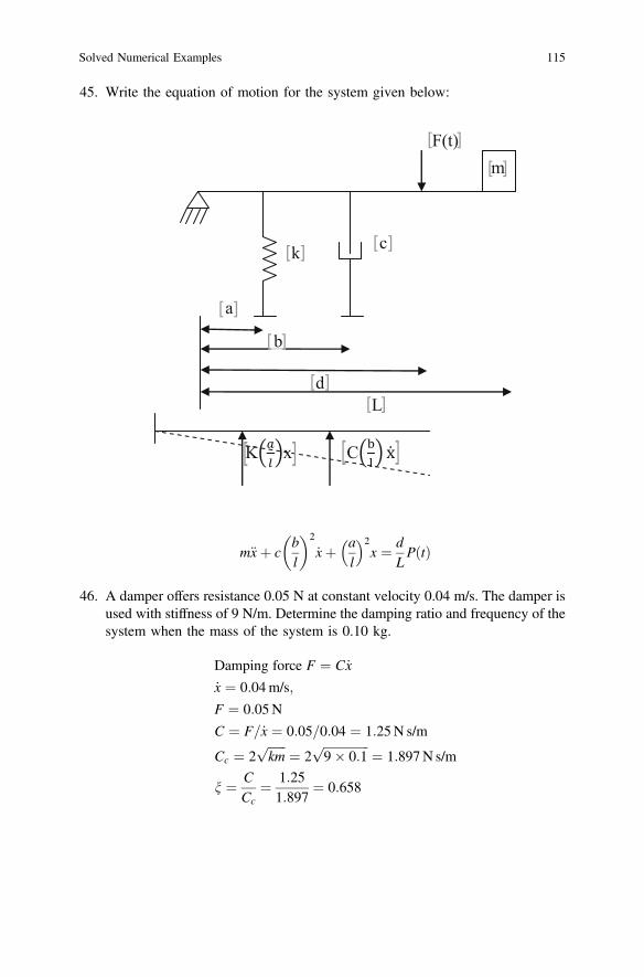
45. Write the equation of motion for the system given below:
[ ]
[ ]
[ ][ ]
[ ]
[ ]
[ ][ ]
[ ][ ]
m€xþ cbl
� �2
_xþ al
� �2x ¼ d
LPðtÞ
46. A damper offers resistance 0.05 N at constant velocity 0.04 m/s. The damper isused with stiffness of 9 N/m. Determine the damping ratio and frequency of thesystem when the mass of the system is 0.10 kg.
Damping force F ¼ C _x
_x ¼ 0:04m/s;
F ¼ 0:05N
C ¼ F=_x ¼ 0:05=0:04 ¼ 1:25N s/m
Cc ¼ 2ffiffiffiffiffiffikm
p¼ 2
ffiffiffiffiffiffiffiffiffiffiffiffiffiffiffi9 0:1
p¼ 1:897N s/m
n ¼ CCc
¼ 1:251:897
¼ 0:658
Solved Numerical Examples 115
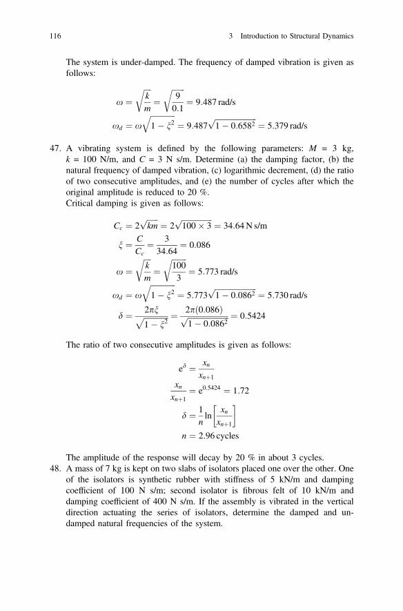
The system is under-damped. The frequency of damped vibration is given asfollows:
x ¼ffiffiffiffikm
r¼
ffiffiffiffiffiffiffi90:1
r¼ 9:487 rad/s
xd ¼ xffiffiffiffiffiffiffiffiffiffiffiffiffi1� n2
q¼ 9:487
ffiffiffiffiffiffiffiffiffiffiffiffiffiffiffiffiffiffiffiffiffiffi1� 0:6582
p¼ 5:379 rad/s
47. A vibrating system is defined by the following parameters: M = 3 kg,k = 100 N/m, and C = 3 N s/m. Determine (a) the damping factor, (b) thenatural frequency of damped vibration, (c) logarithmic decrement, (d) the ratioof two consecutive amplitudes, and (e) the number of cycles after which theoriginal amplitude is reduced to 20 %.Critical damping is given as follows:
Cc ¼ 2ffiffiffiffiffiffikm
p¼ 2
ffiffiffiffiffiffiffiffiffiffiffiffiffiffiffiffi100 3
p¼ 34:64N s/m
n ¼ CCc
¼ 334:64
¼ 0:086
x ¼ffiffiffiffikm
r¼
ffiffiffiffiffiffiffiffi1003
r¼ 5:773 rad/s
xd ¼ xffiffiffiffiffiffiffiffiffiffiffiffiffi1� n2
q¼ 5:773
ffiffiffiffiffiffiffiffiffiffiffiffiffiffiffiffiffiffiffiffiffiffi1� 0:0862
p¼ 5:730 rad/s
d ¼ 2pnffiffiffiffiffiffiffiffiffiffiffiffiffi1� n2
p ¼ 2pð0:086Þffiffiffiffiffiffiffiffiffiffiffiffiffiffiffiffiffiffiffiffiffiffi1� 0:0862
p ¼ 0:5424
The ratio of two consecutive amplitudes is given as follows:
ed ¼ xnxnþ1
xnxnþ1
¼ e0:5424 ¼ 1:72
d ¼ 1nln
xnxnþ1
� �n ¼ 2:96 cycles
The amplitude of the response will decay by 20 % in about 3 cycles.48. A mass of 7 kg is kept on two slabs of isolators placed one over the other. One
of the isolators is synthetic rubber with stiffness of 5 kN/m and dampingcoefficient of 100 N s/m; second isolator is fibrous felt of 10 kN/m anddamping coefficient of 400 N s/m. If the assembly is vibrated in the verticaldirection actuating the series of isolators, determine the damped and un-damped natural frequencies of the system.
116 3 Introduction to Structural Dynamics
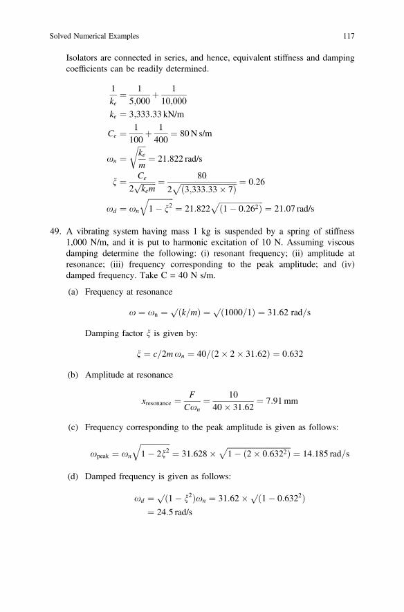
Isolators are connected in series, and hence, equivalent stiffness and dampingcoefficients can be readily determined.
1ke
¼ 15;000
þ 110;000
ke ¼ 3;333:33 kN/m
Ce ¼ 1100
þ 1400
¼ 80N s/m
xn ¼ffiffiffiffikem
r¼ 21:822 rad/s
n ¼ Ce
2ffiffiffiffiffiffiffiffikem
p ¼ 80
2ffiffiffiffiffiffiffiffiffiffiffiffiffiffiffiffiffiffiffiffiffiffiffiffiffiffiffiffiffið3;333:33 7Þp ¼ 0:26
xd ¼ xn
ffiffiffiffiffiffiffiffiffiffiffiffiffi1� n2
q¼ 21:822
ffiffiffiffiffiffiffiffiffiffiffiffiffiffiffiffiffiffiffiffiffiffiffið1� 0:262Þ
p¼ 21:07 rad/s
49. A vibrating system having mass 1 kg is suspended by a spring of stiffness1,000 N/m, and it is put to harmonic excitation of 10 N. Assuming viscousdamping determine the following: (i) resonant frequency; (ii) amplitude atresonance; (iii) frequency corresponding to the peak amplitude; and (iv)damped frequency. Take C = 40 N s/m.
(a) Frequency at resonance
x ¼ xn ¼ pk=mð Þ ¼ p
1000=1ð Þ ¼ 31:62 rad=s
Damping factor n is given by:
n ¼ c=2mxn ¼ 40=ð2 2 31:62Þ ¼ 0:632
(b) Amplitude at resonance
xresonance ¼ FCxn
¼ 1040 31:62
¼ 7:91mm
(c) Frequency corresponding to the peak amplitude is given as follows:
xpeak ¼ xn
ffiffiffiffiffiffiffiffiffiffiffiffiffiffiffi1� 2n2
q¼ 31:628
ffiffiffiffiffiffiffiffiffiffiffiffiffiffiffiffiffiffiffiffiffiffiffiffiffiffiffiffiffiffiffiffiffi1� ð2 0:6322Þ
p¼ 14:185 rad=s
(d) Damped frequency is given as follows:
xd ¼ pð1� n2Þxn ¼ 31:62pð1� 0:6322Þ¼ 24:5 rad/s
Solved Numerical Examples 117

50. A body of mass 70 kg is suspended from a spring which deflects 2 cm underthe load. It is subjected to damping whose value is tuned to be 0.23 times of thevalue that required for critical damping. Find the natural frequency of the un-damped and damped vibrations and ratio of successive amplitudes for dampedvibrations. If the body is subjected to a periodic disturbing force of 700 N andof frequency equal to 0.78 the natural un-damped frequency, find the amplitudeof forced vibrations and the phase difference with respect to the disturbingforce.Spring stiffness k ¼ force=deflection ¼ ð70 9:81Þ=ð2 10�2Þ ¼ 34; 335N/m
n ¼ C=Cc ¼ 0:23
Un-damped natural frequency is given as follows:
xn ¼ffiffiffiffikm
r¼
ffiffiffiffiffiffiffiffiffiffiffiffiffiffiffiffiffiffiffiffiffiffiffiffiffiffiffiffiffiffið34:335 103Þ
70
r¼ 22:15 rad/s
Damped natural frequency is given as follows:
xd ¼ pð1� n2Þxn
¼ 22:15ffiffiffiffiffiffiffiffiffiffiffiffiffiffiffiffiffiffiffiffiffiffiffið1� 0:232Þ
p¼ 21:57 rad/s
Logarithmic decrement is given as follows:
d ¼ 2pn=pð1� n2Þ
¼ 2p 0:23=ffiffiffiffiffiffiffiffiffiffiffiffiffiffiffiffiffiffiffiffiffiffiffið1� 0:232Þ
p¼ 1:48
Ratio of successive amplitudes is given as follows:
A1
A2¼ ed ¼ e1:48 ¼ 4:39
The relation is valid. Hence,
A= F=kð Þ ¼ 1ffiffiffiffiffiffiffiffiffiffiffiffiffiffiffiffiffiffiffiffiffiffiffiffið1� b2Þ2 þ
qð2 n bÞ2
Given that F = 700 N, k = 34.335 × 10³ N/m, β = 0.78
A ¼700
34;335ffiffiffiffiffiffiffiffiffiffiffiffiffiffiffiffiffiffiffiffiffiffiffiffiffiffiffiffiffiffið1� 0:782Þ2 þ
qð2 0:23 0:78Þ2
¼ 0:038m
118 3 Introduction to Structural Dynamics
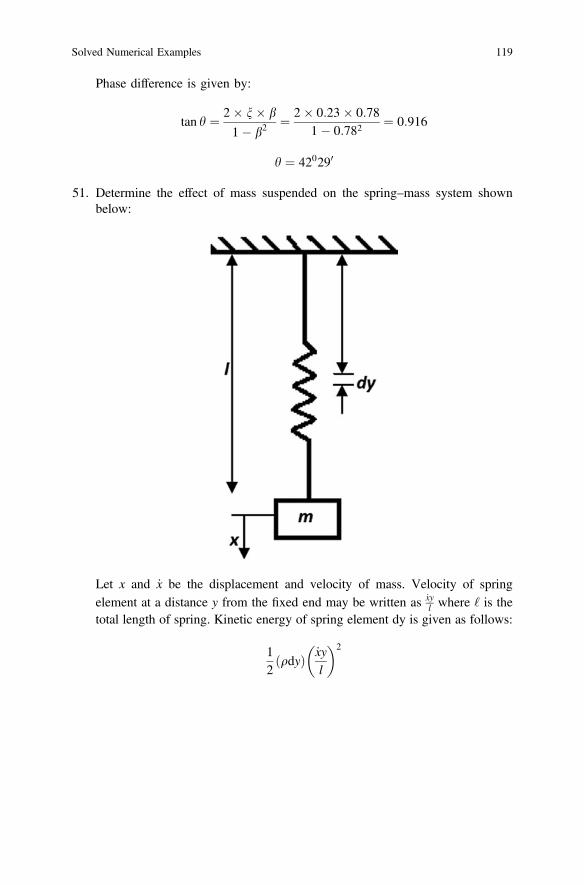
Phase difference is given by:
tan h ¼ 2 n b
1� b2¼ 2 0:23 0:78
1� 0:782¼ 0:916
h ¼ 420290
51. Determine the effect of mass suspended on the spring–mass system shownbelow:
Let x and _x be the displacement and velocity of mass. Velocity of springelement at a distance y from the fixed end may be written as _xy
l where ‘ is thetotal length of spring. Kinetic energy of spring element dy is given as follows:
12
qdyð Þ _xyl
� �2
Solved Numerical Examples 119
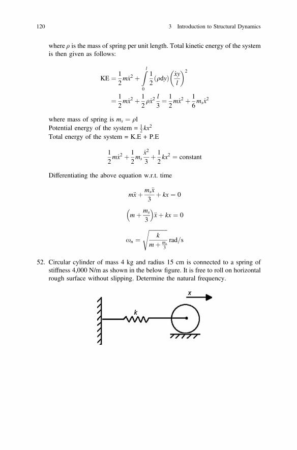
where ρ is the mass of spring per unit length. Total kinetic energy of the systemis then given as follows:
KE ¼ 12m _x2 þ
Z l
0
12
qdyð Þ _xyl
� �2
¼ 12m _x2 þ 1
2q _x2
l3¼ 1
2m _x2 þ 1
6ms _x
2
where mass of spring is ms ¼ qlPotential energy of the system = 1
2 kx2
Total energy of the system = K.E + P.E
12m _x2 þ 1
2ms
_x2
3þ 12kx2 ¼ constant
Differentiating the above equation w.r.t. time
m€xþ ms€x3
þ kx ¼ 0
mþ ms
3
� �€xþ kx ¼ 0
xn ¼ffiffiffiffiffiffiffiffiffiffiffiffiffi
kmþ ms
3
srad=s
52. Circular cylinder of mass 4 kg and radius 15 cm is connected to a spring ofstiffness 4,000 N/m as shown in the below figure. It is free to roll on horizontalrough surface without slipping. Determine the natural frequency.
120 3 Introduction to Structural Dynamics
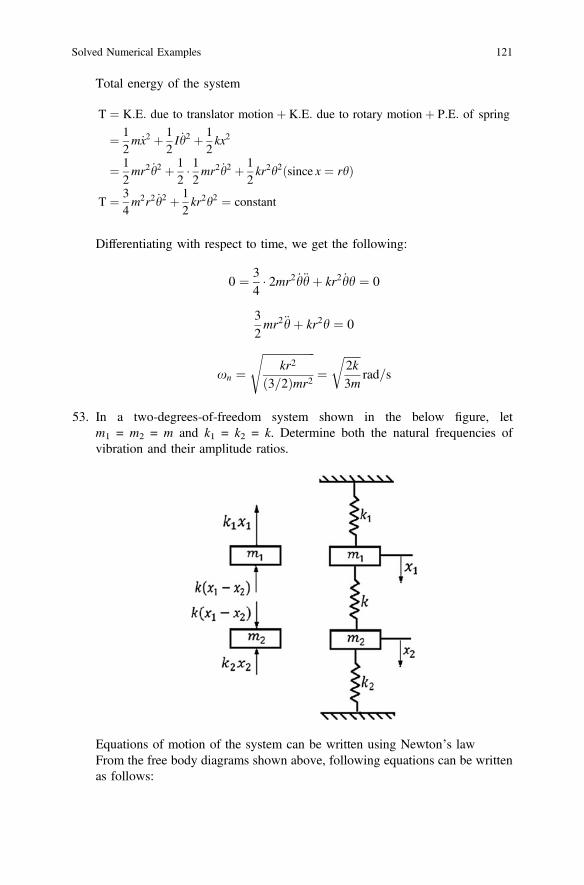
Total energy of the system
T ¼ K:E: due to translator motionþ K:E: due to rotary motionþ P:E: of spring
¼ 12m _x2 þ 1
2I _h2 þ 1
2kx2
¼ 12mr2 _h2 þ 1
2� 12mr2 _h2 þ 1
2kr2h2ðsince x ¼ rhÞ
T ¼ 34m2r2 _h2 þ 1
2kr2h2 ¼ constant
Differentiating with respect to time, we get the following:
0 ¼ 34� 2mr2 _h€hþ kr2 _hh ¼ 0
32mr2€hþ kr2h ¼ 0
xn ¼ffiffiffiffiffiffiffiffiffiffiffiffiffiffiffiffiffiffiffi
kr2
ð3=2Þmr2
s¼
ffiffiffiffiffiffi2k3m
rrad=s
53. In a two-degrees-of-freedom system shown in the below figure, letm1 = m2 = m and k1 = k2 = k. Determine both the natural frequencies ofvibration and their amplitude ratios.
Equations of motion of the system can be written using Newton’s lawFrom the free body diagrams shown above, following equations can be writtenas follows:
Solved Numerical Examples 121
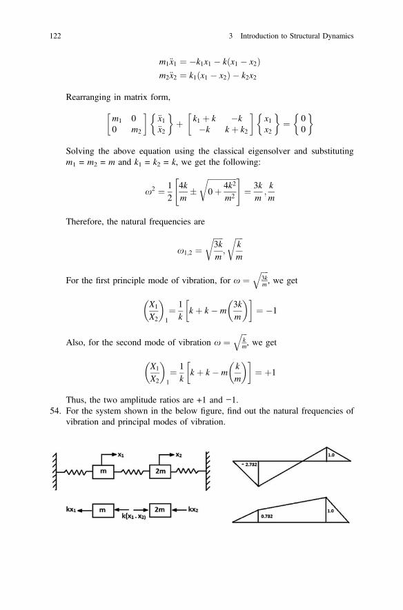
m1€x1 ¼ �k1x1 � kðx1 � x2Þm2€x2 ¼ k1ðx1 � x2Þ � k2x2
Rearranging in matrix form,
m1 00 m2
� �€x1€x2
� �þ k1 þ k �k
�k k þ k2
� �x1x2
� �¼ 0
0
� �
Solving the above equation using the classical eigensolver and substitutingm1 = m2 = m and k1 = k2 = k, we get the following:
x2 ¼ 12
4km
�ffiffiffiffiffiffiffiffiffiffiffiffiffiffiffi0þ 4k2
m2
r" #¼ 3k
m;km
Therefore, the natural frequencies are
x1;2 ¼ffiffiffiffiffi3km
r;
ffiffiffiffikm
r
For the first principle mode of vibration, for x ¼ffiffiffiffi3km
q, we get
X1
X2
� �1¼ 1
kk þ k � m
3km
� �� �¼ �1
Also, for the second mode of vibration x ¼ffiffiffikm
q, we get
X1
X2
� �1¼ 1
kk þ k � m
km
� �� �¼ þ1
Thus, the two amplitude ratios are +1 and −1.54. For the system shown in the below figure, find out the natural frequencies of
vibration and principal modes of vibration.
122 3 Introduction to Structural Dynamics
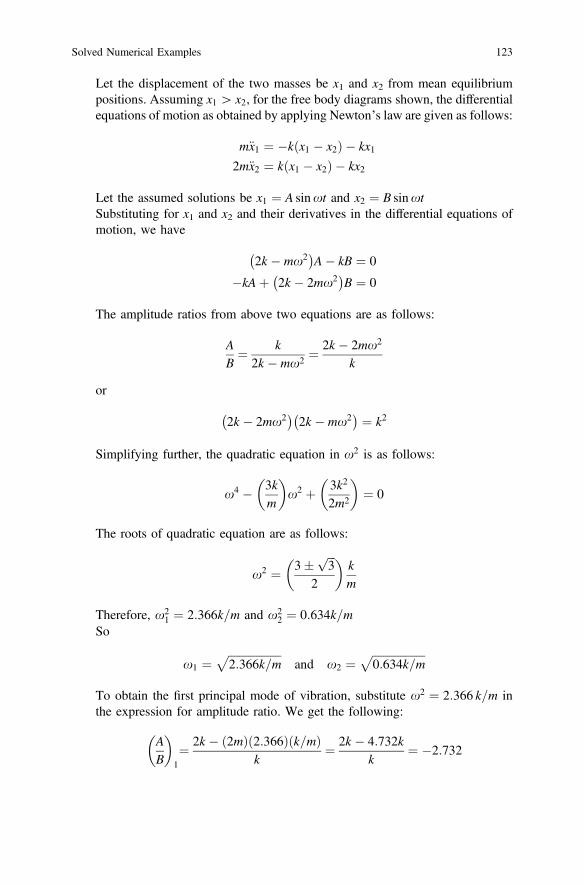
Let the displacement of the two masses be x1 and x2 from mean equilibriumpositions. Assuming x1 [ x2, for the free body diagrams shown, the differentialequations of motion as obtained by applying Newton’s law are given as follows:
m€x1 ¼ �k x1 � x2ð Þ � kx12m€x2 ¼ k x1 � x2ð Þ � kx2
Let the assumed solutions be x1 ¼ A sinxt and x2 ¼ B sinxtSubstituting for x1 and x2 and their derivatives in the differential equations ofmotion, we have
2k � mx2� �A� kB ¼ 0
�kAþ 2k � 2mx2� �B ¼ 0
The amplitude ratios from above two equations are as follows:
AB¼ k
2k � mx2 ¼2k � 2mx2
k
or
2k � 2mx2� �2k � mx2� � ¼ k2
Simplifying further, the quadratic equation in x2 is as follows:
x4 � 3km
� �x2 þ 3k2
2m2
� �¼ 0
The roots of quadratic equation are as follows:
x2 ¼ 3� ffiffiffi3
p
2
� �km
Therefore, x21 ¼ 2:366k=m and x2
2 ¼ 0:634k=mSo
x1 ¼ffiffiffiffiffiffiffiffiffiffiffiffiffiffiffiffiffiffiffi2:366k=m
pand x2 ¼
ffiffiffiffiffiffiffiffiffiffiffiffiffiffiffiffiffiffiffi0:634k=m
pTo obtain the first principal mode of vibration, substitute x2 ¼ 2:366 k=m inthe expression for amplitude ratio. We get the following:
AB
� �1¼ 2k � 2mð Þ 2:366ð Þðk=mÞ
k¼ 2k � 4:732k
k¼ �2:732
Solved Numerical Examples 123
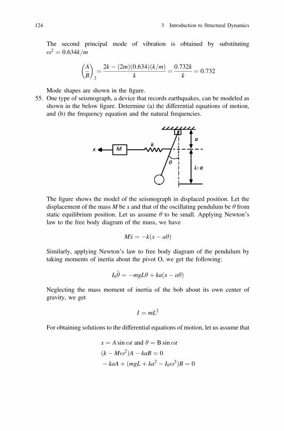
The second principal mode of vibration is obtained by substitutingx2 ¼ 0:634k=m
AB
� �2¼ 2k � 2mð Þ 0:634ð Þðk=mÞ
k¼ 0:732k
k¼ 0:732
Mode shapes are shown in the figure.55. One type of seismograph, a device that records earthquakes, can be modeled as
shown in the below figure. Determine (a) the differential equations of motion,and (b) the frequency equation and the natural frequencies.
The figure shows the model of the seismograph in displaced position. Let thedisplacement of the massM be x and that of the oscillating pendulum be θ fromstatic equilibrium position. Let us assume θ to be small. Applying Newton’slaw to the free body diagram of the mass, we have
M€x ¼ �kðx� ahÞ
Similarly, applying Newton’s law to free body diagram of the pendulum bytaking moments of inertia about the pivot O, we get the following:
I0€h ¼ �mgLhþ kaðx� ahÞ
Neglecting the mass moment of inertia of the bob about its own center ofgravity, we get
I ¼ mL2
For obtaining solutions to the differential equations of motion, let us assume that
x ¼ A sinxt and h ¼ B sinxt
ðk �Mx2ÞA� kaB ¼ 0
� kaAþ ðmgLþ ka2 � I0x2ÞB ¼ 0
124 3 Introduction to Structural Dynamics
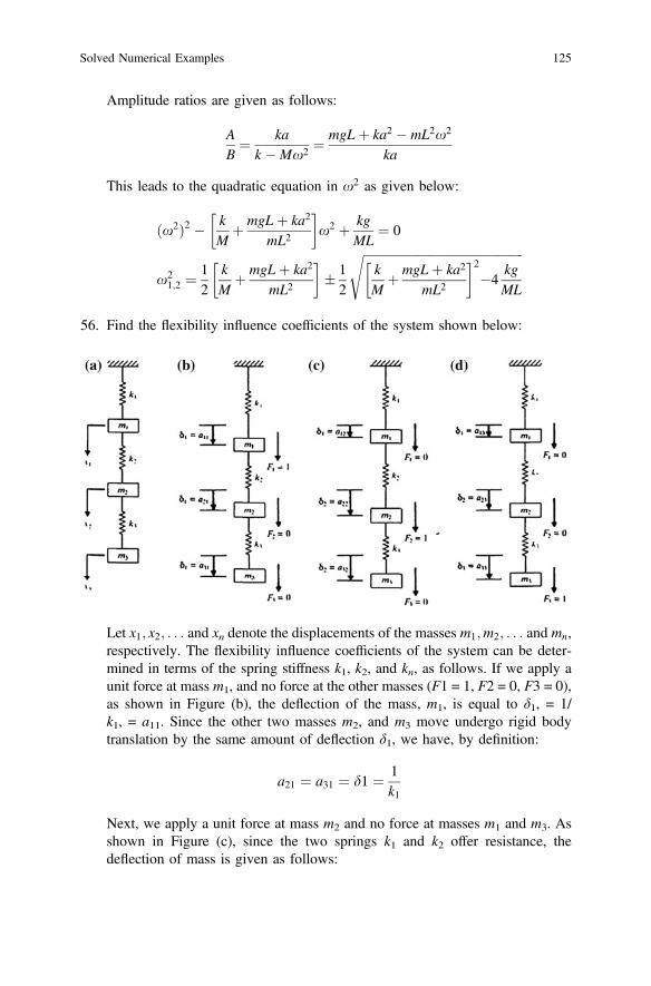
Amplitude ratios are given as follows:
AB¼ ka
k �Mx2 ¼mgLþ ka2 � mL2x2
ka
This leads to the quadratic equation in x2 as given below:
ðx2Þ2 � kM
þ mgLþ ka2
mL2
� �x2 þ kg
ML¼ 0
x21;2 ¼
12
kM
þ mgLþ ka2
mL2
� �� 12
ffiffiffiffiffiffiffiffiffiffiffiffiffiffiffiffiffiffiffiffiffiffiffiffiffiffiffiffiffiffiffiffiffiffiffiffiffiffiffiffiffiffiffiffiffiffiffiffiffiffiffiffikM
þ mgLþ ka2
mL2
� �2�4
kgML
s
56. Find the flexibility influence coefficients of the system shown below:
Let x1; x2; . . . and xn denote the displacements of the masses m1;m2; . . . and mn,respectively. The flexibility influence coefficients of the system can be deter-mined in terms of the spring stiffness k1, k2, and kn, as follows. If we apply aunit force at mass m1, and no force at the other masses (F1 = 1, F2 = 0, F3 = 0),as shown in Figure (b), the deflection of the mass, m1, is equal to δ1, = 1/k1, = a11. Since the other two masses m2, and m3 move undergo rigid bodytranslation by the same amount of deflection δ1, we have, by definition:
a21 ¼ a31 ¼ d1 ¼ 1k1
Next, we apply a unit force at mass m2 and no force at masses m1 and m3. Asshown in Figure (c), since the two springs k1 and k2 offer resistance, thedeflection of mass is given as follows:
Solved Numerical Examples 125
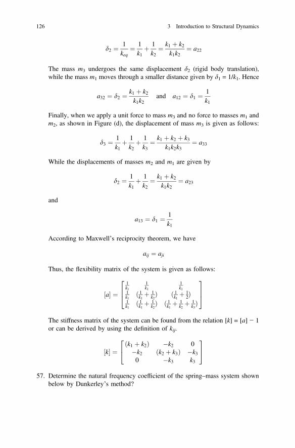
d2 ¼ 1keq
¼ 1k1
þ 1k2
¼ k1 þ k2k1k2
¼ a22
The mass m3 undergoes the same displacement δ2 (rigid body translation),while the mass m1 moves through a smaller distance given by δ1 = 1/k1. Hence
a32 ¼ d2 ¼ k1 þ k2k1k2
and a12 ¼ d1 ¼ 1k1
Finally, when we apply a unit force to mass m3 and no force to masses m1 andm2, as shown in Figure (d), the displacement of mass m3 is given as follows:
d3 ¼ 1k1
þ 1k2
þ 1k3
¼ k1 þ k2 þ k3k1k2k3
¼ a33
While the displacements of masses m2 and m1 are given by
d2 ¼ 1k1
þ 1k2
¼ k1 þ k2k1k2
¼ a23
and
a13 ¼ d1 ¼ 1k1
According to Maxwell’s reciprocity theorem, we have
aij ¼ aji
Thus, the flexibility matrix of the system is given as follows:
½a� ¼1k1
1k1
1k1
1k1
ð 1k1 þ 1k2Þ ð 1k1 þ 1
2Þ1k1
ð 1k1 þ 1k2Þ ð 1k1 þ 1
k2þ 1
k3Þ
264
375
The stiffness matrix of the system can be found from the relation [k] = [a] − 1or can be derived by using the definition of kij.
½k� ¼ðk1 þ k2Þ �k2 0
�k2 ðk2 þ k3Þ �k30 �k3 k3
24
35
57. Determine the natural frequency coefficient of the spring–mass system shownbelow by Dunkerley’s method?
126 3 Introduction to Structural Dynamics
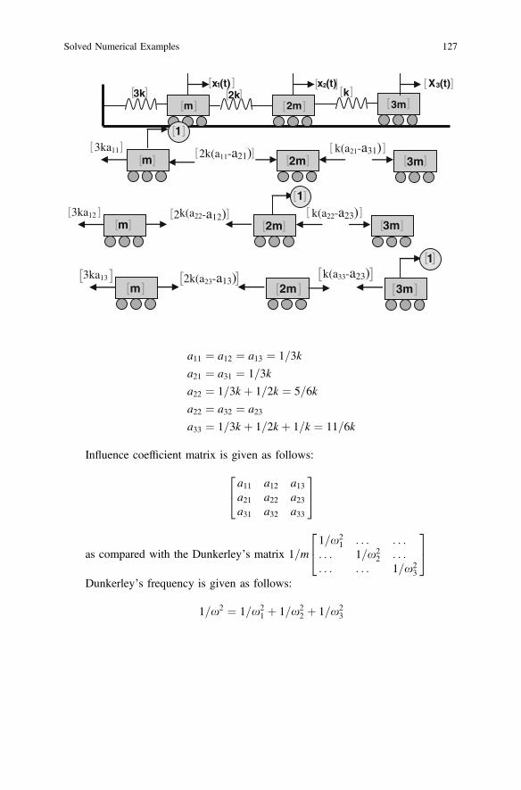
x1(t)3k 2k k
x2(t)
m 2m 3m
X3(t)
m
1
2m 3m3ka11 2k(a11-a21) k(a21-a31)
m
1
2m 3m3ka12 2k(a22-a12) k(a22-a23)
[ ][ ]
[ ][ ]
[ ][ ]
[ ]
[ ]
[ ][ ][ ]
[ ]
[ ][ ]
[ ][ ]
[ ]
[ ]
[ ][ ]
[ ]
[ ]
[ ]
m
1
2m 3m3ka13 2k(a23-a13) k(a33-a23)
[ ] [ ] [ ]
[ ][ ][ ][ ]
a11 ¼ a12 ¼ a13 ¼ 1=3k
a21 ¼ a31 ¼ 1=3k
a22 ¼ 1=3k þ 1=2k ¼ 5=6k
a22 ¼ a32 ¼ a23a33 ¼ 1=3k þ 1=2k þ 1=k ¼ 11=6k
Influence coefficient matrix is given as follows:
a11 a12 a13a21 a22 a23a31 a32 a33
24
35
as compared with the Dunkerley’s matrix 1=m1=x2
1 . . . . . .. . . 1=x2
2 . . .. . . . . . 1=x2
3
24
35
Dunkerley’s frequency is given as follows:
1=x2 ¼ 1=x21 þ 1=x2
2 þ 1=x23
Solved Numerical Examples 127
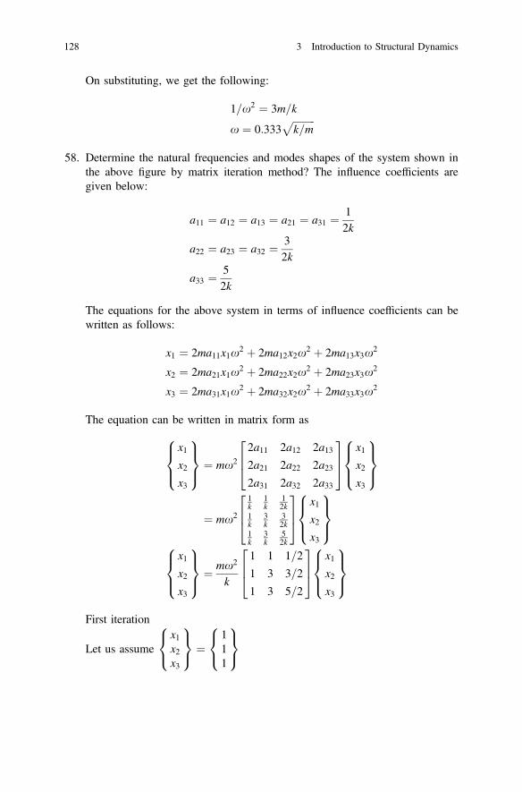
On substituting, we get the following:
1=x2 ¼ 3m=k
x ¼ 0:333ffiffiffiffiffiffiffiffiffik=m
p58. Determine the natural frequencies and modes shapes of the system shown in
the above figure by matrix iteration method? The influence coefficients aregiven below:
a11 ¼ a12 ¼ a13 ¼ a21 ¼ a31 ¼ 12k
a22 ¼ a23 ¼ a32 ¼ 32k
a33 ¼ 52k
The equations for the above system in terms of influence coefficients can bewritten as follows:
x1 ¼ 2ma11x1x2 þ 2ma12x2x2 þ 2ma13x3x2
x2 ¼ 2ma21x1x2 þ 2ma22x2x2 þ 2ma23x3x2
x3 ¼ 2ma31x1x2 þ 2ma32x2x2 þ 2ma33x3x2
The equation can be written in matrix form as
x1x2x3
8><>:
9>=>; ¼ mx2
2a11 2a12 2a132a21 2a22 2a232a31 2a32 2a33
264
375
x1x2x3
8><>:
9>=>;
¼ mx2
1k
1k
12k
1k
3k
32k
1k
3k
52k
264
375
x1x2x3
8><>:
9>=>;
x1x2x3
8><>:
9>=>; ¼ mx2
k
1 1 1=2
1 3 3=2
1 3 5=2
264
375
x1x2x3
8><>:
9>=>;
First iteration
Let us assumex1x2x3
8<:
9=; ¼
111
8<:
9=;
128 3 Introduction to Structural Dynamics

111
8<:
9=; ¼ mx2
k
1 1 1=21 3 3=21 3 5=2
24
35 ¼ 2:5
mx2
k
12:22:6
8<:
9=;
Second iteration
12:22:6
8<:
9=; ¼ mx2
k
1 1 1=21 3 3=21 3 5=2
24
35 1
2:22:6
8<:
9=; ¼ 4:5
mx2
k
12:5553:133
8<:
9=;
Third iteration
12:5553:133
8<:
9=; ¼ mx2
k
1 1 1=21 3 3=21 3 5=2
24
35 1
2:5553:133
8<:
9=; ¼ 5:12
mx2
k
12:613:22
8<:
9=;
Fourth iteration
12:613:22
8<:
9=; ¼ mx2
k
1 1 1=21 3 3=21 3 5=2
24
35 1
2:613:22
8<:
9=; ¼ 5:22
mx2
k
12:613:23
8<:
9=;
So
1 ¼ 5:22mx2
k; x2 ¼ 1
5:22km
Thus x1 ¼ 0:437ffiffiffikm
q.
To find the second principle mode, the orthogonality relation is used as
x1x2x3
8><>:
9>=>; ¼ mx2
k
1 1 1=2
1 3 3=2
1 3 5=2
264
375 0 �m2
m1
x2x1
� ��m3m1
x3x1
� �0 1 0
0 0 1
2664
3775
x1x2x3
8><>:
9>=>;
¼ mx2
k
1 1 1=2
1 3 3=2
1 3 5=2
264
375
0 � 2:611
� � � 12 3:23ð Þ
0 1 0
0 0 1
264
375
x1x2x3
8><>:
9>=>;
¼ mx2
k
0 �1:61 �1:11
0 0:39 �0:11
0 0:39 1:89
264
375
x1x2x3
8><>:
9>=>;
Solved Numerical Examples 129
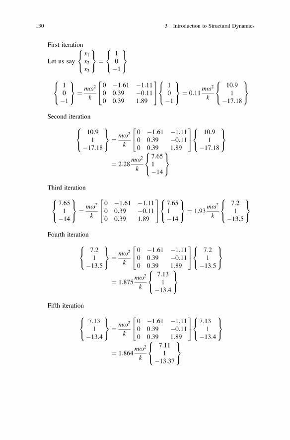
First iteration
Let us sayx1x2x3
8<:
9=; ¼
10�1
8<:
9=;
10�1
8<:
9=; ¼ mx2
k
0 �1:61 �1:110 0:39 �0:110 0:39 1:89
24
35 1
0�1
8<:
9=; ¼ 0:11
mx2
k
10:91
�17:18
8<:
9=;
Second iteration
10:91
�17:18
8<:
9=; ¼ mx2
k
0 �1:61 �1:110 0:39 �0:110 0:39 1:89
24
35 10:9
1�17:18
8<:
9=;
¼ 2:28mx2
k
7:651�14
8<:
9=;
Third iteration
7:651
�14
8<:
9=; ¼ mx2
k
0 �1:61 �1:110 0:39 �0:110 0:39 1:89
24
35 7:65
1�14
8<:
9=; ¼ 1:93
mx2
k
7:21
�13:5
8<:
9=;
Fourth iteration
7:21
�13:5
8<:
9=; ¼ mx2
k
0 �1:61 �1:110 0:39 �0:110 0:39 1:89
24
35 7:2
1�13:5
8<:
9=;
¼ 1:875mx2
k
7:131
�13:4
8<:
9=;
Fifth iteration
7:131
�13:4
8<:
9=; ¼ mx2
k
0 �1:61 �1:110 0:39 �0:110 0:39 1:89
24
35 7:13
1�13:4
8<:
9=;
¼ 1:864mx2
k
7:111
�13:37
8<:
9=;
130 3 Introduction to Structural Dynamics
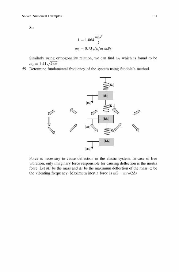
So
1 ¼ 1:864mx2
kx2 ¼ 0:73
ffiffiffiffiffiffiffiffiffik=m
prad/s
Similarly using orthogonality relation, we can find x3 which is found to bex3 ¼ 1:41
ffiffiffiffiffiffiffiffiffik=m
p59. Determine fundamental frequency of the system using Stodola’s method.
K1
K2
K3
M1
M2
M3
x1
x2
x3
[ ]
[ ]
[ ]
[ ]
[ ]
[ ]
[ ]
[ ]
[ ]
Force is necessary to cause deflection in the elastic system. In case of freevibration, only imaginary force responsible for causing deflection is the inertiaforce. Let Mr be the mass and Δr be the maximum deflection of the mass. ω bethe vibrating frequency. Maximum inertia force is m€x ¼ mrx2Dr
Solved Numerical Examples 131
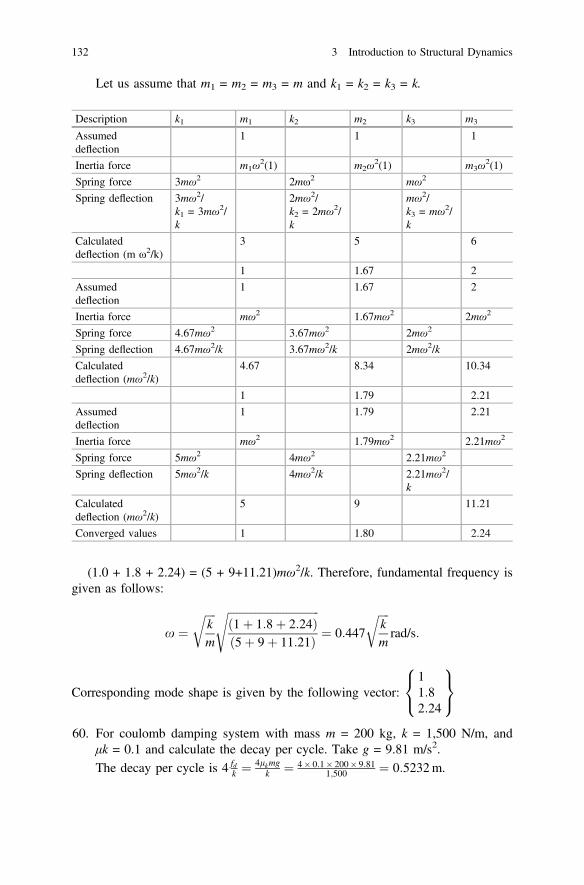
Let us assume that m1 = m2 = m3 = m and k1 = k2 = k3 = k.
(1.0 + 1.8 + 2.24) = (5 + 9+11.21)mω2/k. Therefore, fundamental frequency isgiven as follows:
x ¼ffiffiffiffikm
r ffiffiffiffiffiffiffiffiffiffiffiffiffiffiffiffiffiffiffiffiffiffiffiffiffiffiffiffiffiffiffiffiffið1þ 1:8þ 2:24Þð5þ 9þ 11:21Þ
s¼ 0:447
ffiffiffiffikm
rrad/s:
Corresponding mode shape is given by the following vector:11:82:24
8<:
9=;
60. For coulomb damping system with mass m = 200 kg, k = 1,500 N/m, andμk = 0.1 and calculate the decay per cycle. Take g = 9.81 m/s2.The decay per cycle is 4 fd
k ¼ 4lkmgk ¼ 4 0:1 200 9:81
1;500 ¼ 0:5232m.
Description k1 m1 k2 m2 k3 m3
Assumeddeflection
1 1 1
Inertia force m1ω2(1) m2ω
2(1) m3ω2(1)
Spring force 3mω2 2mω2 mω2
Spring deflection 3mω2/k1 = 3mω2/k
2mω2/k2 = 2mω2/k
mω2/k3 = mω2/k
Calculateddeflection (m ω2/k)
3 5 6
1 1.67 2
Assumeddeflection
1 1.67 2
Inertia force mω2 1.67mω2 2mω2
Spring force 4.67mω2 3.67mω2 2mω2
Spring deflection 4.67mω2/k 3.67mω2/k 2mω2/k
Calculateddeflection (mω2/k)
4.67 8.34 10.34
1 1.79 2.21
Assumeddeflection
1 1.79 2.21
Inertia force mω2 1.79mω2 2.21mω2
Spring force 5mω2 4mω2 2.21mω2
Spring deflection 5mω2/k 4mω2/k 2.21mω2/k
Calculateddeflection (mω2/k)
5 9 11.21
Converged values 1 1.80 2.24
132 3 Introduction to Structural Dynamics
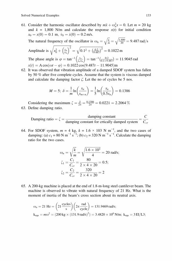
61. Consider the harmonic oscillator described by m€xþ x2nx ¼ 0. Let m = 20 kg
and k = 1,800 N/m and calculate the response x(t) for initial conditionx0 ¼ xð0Þ ¼ 0:1 m; _v0 ¼ _xð0Þ ¼ 0:2m/s.
The natural frequency of the oscillator is xn ¼ffiffiffikm
q¼
ffiffiffiffiffiffiffiffi1;80020
q¼ 9:487 rad=s
Amplitude is
ffiffiffiffiffiffiffiffiffiffiffiffiffiffiffiffiffiffiffiffiffiffix20 þ vo
xn
� �2r¼
ffiffiffiffiffiffiffiffiffiffiffiffiffiffiffiffiffiffiffiffiffiffiffiffiffiffiffiffi0:12 þ 0:2
9:487
� �2q¼ 0:1022m
The phase angle is u ¼ tan�1 voxoxn
� �¼ tan�1 0:2
0:19:487
� � ¼ 11:9045 rad
xðtÞ ¼ Acos xt � uð Þ ¼ 0:1022 cos 9:487t � 11:9045ð Þm62. It was observed that vibration amplitude of a damped SDOF system has fallen
by 50 % after five complete cycles. Assume that the system is viscous dampedand calculate the damping factor ζ. Let the no of cycles be 5 nos.
M ¼ 5; d ¼ 1mln
xnxmþn
� �¼ 1
5ln
xn0:5xn
� �¼ 0:1386
Considering the maximum f ¼ d2p ¼ 0:1386
2p ¼ 0:0221 ¼ 2:2064%63. Define damping ratio.
Damping ratio ¼ f ¼ damping constantdamping constant for crtically damped system
¼ CCcr
64. For SDOF system, m = 4 kg, k = 1.6 × 10³ N m−1, and the two cases ofdamping: (a) c1 = 80 N m−1 s−1; (b) c2 = 320 N m−1 s−1. Calculate the dampingratio for the two cases.
xn ¼ffiffiffiffikm
r¼
ffiffiffiffiffiffiffiffiffiffiffiffiffiffiffiffiffiffiffi1:6 103
4
r¼ 20 rad/s;
f1 ¼C1
Ccr¼ 80
2 4 20¼ 0:5;
f2 ¼C2
Ccr¼ 320
2 4 20¼ 2
65. A 200-kg machine is placed at the end of 1.8-m-long steel cantilever beam. Themachine is observed to vibrate with natural frequency of 21 Hz. What is themoment of inertia of the beam’s cross section about its neutral axis.
xn ¼ 21 Hz ¼ 21cycles
s
� �2p
radcycle
� �¼ 131:9469 rad/s;
kequ ¼ mx2 ¼ ð200 kg 131:9 rad/sð Þ2Þ ¼ 3:4820 106 N/m; kequ ¼ 3EI=L3;
Solved Numerical Examples 133
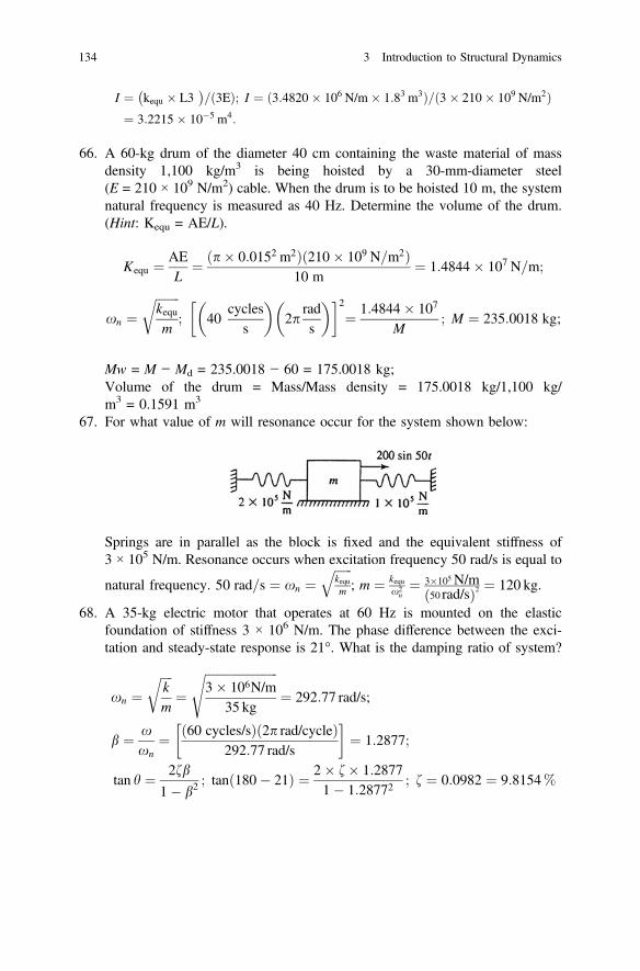
I ¼ kequ L3� �
= 3Eð Þ; I ¼ ð3:4820 106 N/m 1:83 m3Þ=ð3 210 109 N/m2Þ¼ 3:2215 10�5 m4:
66. A 60-kg drum of the diameter 40 cm containing the waste material of massdensity 1,100 kg/m3 is being hoisted by a 30-mm-diameter steel(E = 210 × 109 N/m2) cable. When the drum is to be hoisted 10 m, the systemnatural frequency is measured as 40 Hz. Determine the volume of the drum.(Hint: Kequ = AE/L).
Kequ ¼ AEL
¼ p 0:0152 m2ð Þ 210 109 N=m2ð Þ10 m
¼ 1:4844 107 N=m;
xn ¼ffiffiffiffiffiffiffiffikequm
r; 40
cycless
� �2p
rads
� �� �2¼ 1:4844 107
M; M ¼ 235:0018 kg;
Mw = M − Md = 235.0018 − 60 = 175.0018 kg;Volume of the drum = Mass/Mass density = 175.0018 kg/1,100 kg/m3 = 0.1591 m3
67. For what value of m will resonance occur for the system shown below:
Springs are in parallel as the block is fixed and the equivalent stiffness of3 × 105 N/m. Resonance occurs when excitation frequency 50 rad/s is equal to
natural frequency. 50 rad=s ¼ xn ¼ffiffiffiffiffiffikequm
q; m ¼ kequ
x2n¼ 3105 N/m
50 rad/sð Þ2 ¼ 120 kg.
68. A 35-kg electric motor that operates at 60 Hz is mounted on the elasticfoundation of stiffness 3 × 10⁶ N/m. The phase difference between the exci-tation and steady-state response is 21°. What is the damping ratio of system?
xn ¼ffiffiffiffikm
r¼
ffiffiffiffiffiffiffiffiffiffiffiffiffiffiffiffiffiffiffiffiffiffiffiffi3 106N/m
35 kg
s¼ 292:77 rad/s;
b ¼ xxn
¼ 60 cycles/sð Þ 2p rad/cycleð Þ292:77 rad/s
� �¼ 1:2877;
tan h ¼ 2fb
1� b2; tanð180� 21Þ ¼ 2 f 1:2877
1� 1:28772; f ¼ 0:0982 ¼ 9:8154%
134 3 Introduction to Structural Dynamics
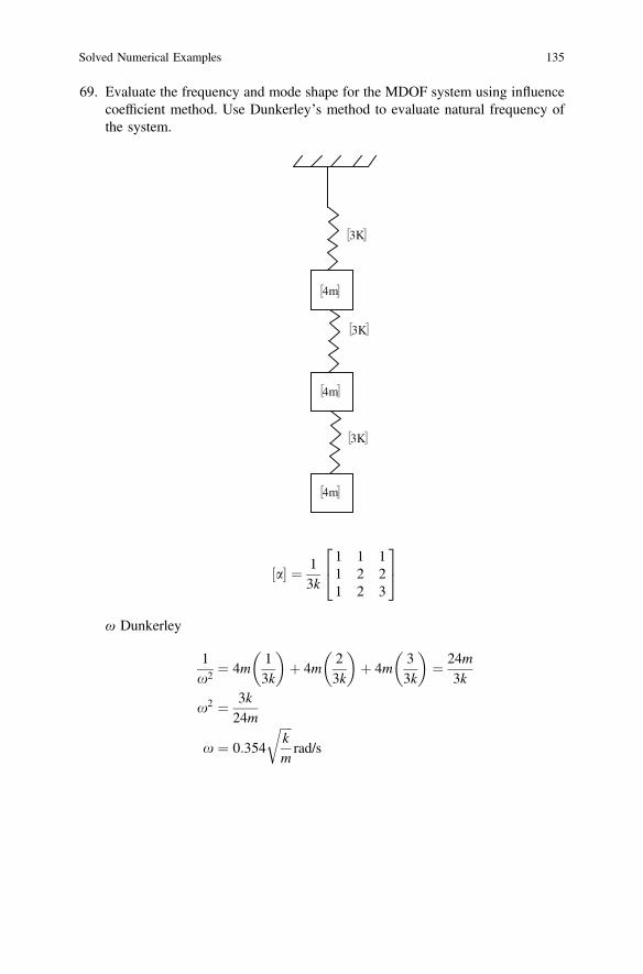
69. Evaluate the frequency and mode shape for the MDOF system using influencecoefficient method. Use Dunkerley’s method to evaluate natural frequency ofthe system.
4m
4m
4m
3K
3K
3K
[ ]
[ ]
[ ]
[ ]
[ ]
[ ]
½a� ¼ 13k
1 1 11 2 21 2 3
24
35
ω Dunkerley
1x2 ¼ 4m
13k
� �þ 4m
23k
� �þ 4m
33k
� �¼ 24m
3k
x2 ¼ 3k24m
x ¼ 0:354
ffiffiffiffikm
rrad/s
Solved Numerical Examples 135
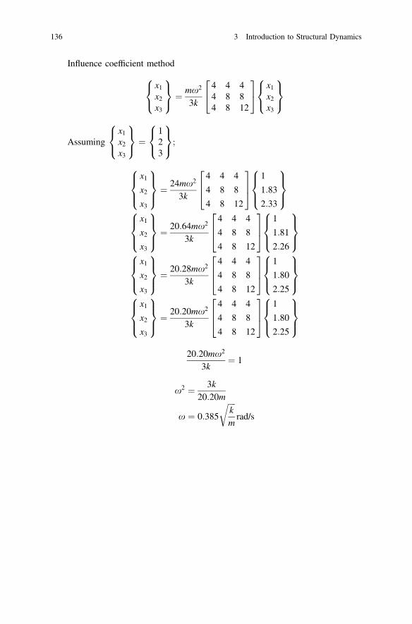
Influence coefficient method
x1x2x3
8<:
9=; ¼ mx2
3k
4 4 44 8 84 8 12
24
35 x1
x2x3
8<:
9=;
Assumingx1x2x3
8<:
9=; ¼
123
8<:
9=;;
x1x2x3
8><>:
9>=>; ¼ 24mx2
3k
4 4 4
4 8 8
4 8 12
264
375
1
1:83
2:33
8><>:
9>=>;
x1x2x3
8><>:
9>=>; ¼ 20:64mx2
3k
4 4 4
4 8 8
4 8 12
264
375
1
1:81
2:26
8><>:
9>=>;
x1x2x3
8><>:
9>=>; ¼ 20:28mx2
3k
4 4 4
4 8 8
4 8 12
264
375
1
1:80
2:25
8><>:
9>=>;
x1x2x3
8><>:
9>=>; ¼ 20:20mx2
3k
4 4 4
4 8 8
4 8 12
264
375
1
1:80
2:25
8><>:
9>=>;
20:20mx2
3k¼ 1
x2 ¼ 3k20:20m
x ¼ 0:385
ffiffiffiffikm
rrad/s
136 3 Introduction to Structural Dynamics
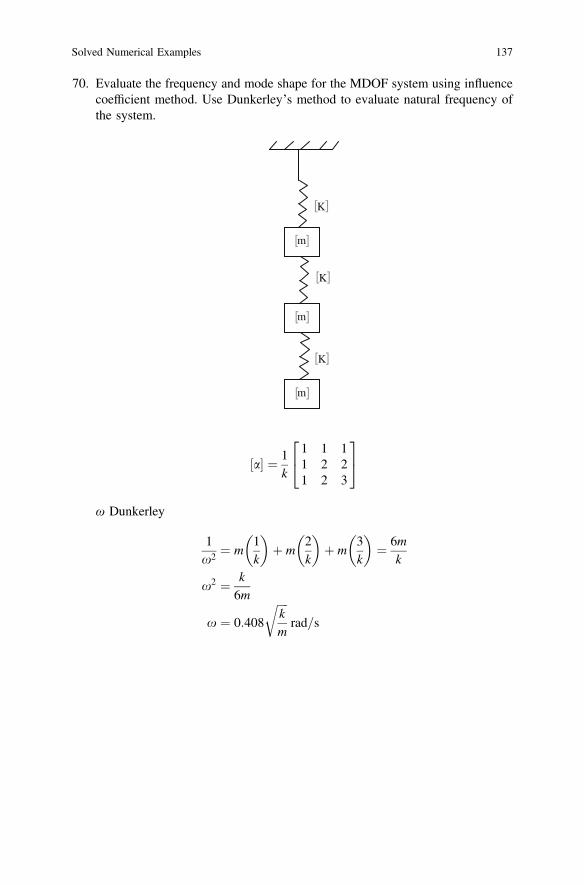
70. Evaluate the frequency and mode shape for the MDOF system using influencecoefficient method. Use Dunkerley’s method to evaluate natural frequency ofthe system.
K
K
K
m
m
m
[ ]
[ ]
[ ]
[ ]
[ ]
[ ]
½a� ¼ 1k
1 1 11 2 21 2 3
24
35
ω Dunkerley
1x2 ¼ m
1k
� �þ m
2k
� �þ m
3k
� �¼ 6m
k
x2 ¼ k6m
x ¼ 0:408
ffiffiffiffikm
rrad=s
Solved Numerical Examples 137
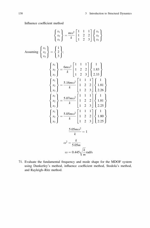
Influence coefficient method
x1x2x3
8<:
9=; ¼ mx2
k
1 1 11 2 21 2 3
24
35 x1
x2x3
8<:
9=;
Assumingx1x2x3
8<:
9=; ¼
123
8<:
9=;;
x1x2x3
8><>:
9>=>; ¼ 6mx2
k
1 1 1
1 2 2
1 2 3
264
375
1
1:83
2:33
8><>:
9>=>;
x1x2x3
8><>:
9>=>; ¼ 5:16mx2
k
1 1 1
1 2 2
1 2 3
264
375
1
1:81
2:26
8><>:
9>=>;
x1x2x3
8><>:
9>=>; ¼ 5:07mx2
k
1 1 1
1 2 2
1 2 3
264
375
1
1:81
2:25
8><>:
9>=>;
x1x2x3
8><>:
9>=>; ¼ 5:05mx2
k
1 1 1
1 2 2
1 2 3
264
375
1
1:80
2:25
8><>:
9>=>;
5:05mx2
k¼ 1
x2 ¼ k5:05m
x ¼ 0:445
ffiffiffiffikm
rrad/s
71. Evaluate the fundamental frequency and mode shape for the MDOF systemusing Dunkerley’s method, influence coefficient method, Stodola’s method,and Rayleigh–Ritz method.
138 3 Introduction to Structural Dynamics
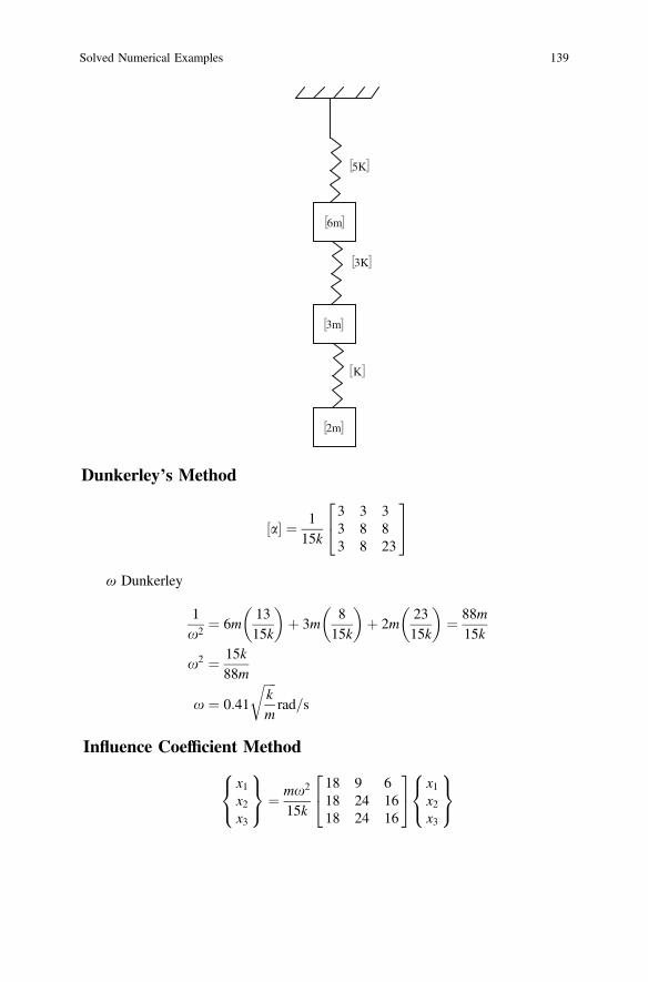
6m
3m
2m
5K
3K
K
[ ]
[ ]
[ ]
[ ]
[ ]
[ ]
Dunkerley’s Method
½a� ¼ 115k
3 3 33 8 83 8 23
24
35
ω Dunkerley
1x2 ¼ 6m
1315k
� �þ 3m
815k
� �þ 2m
2315k
� �¼ 88m
15k
x2 ¼ 15k88m
x ¼ 0:41
ffiffiffiffikm
rrad=s
Influence Coefficient Method
x1x2x3
8<:
9=; ¼ mx2
15k
18 9 618 24 1618 24 16
24
35 x1
x2x3
8<:
9=;
Solved Numerical Examples 139
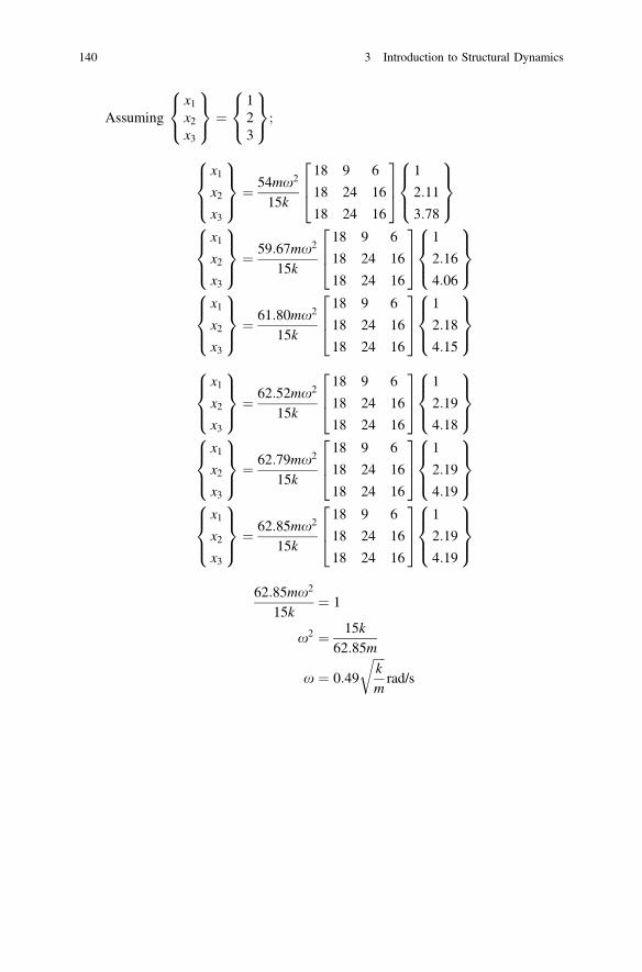
Assumingx1x2x3
8<:
9=; ¼
123
8<:
9=;;
x1x2x3
8><>:
9>=>; ¼ 54mx2
15k
18 9 6
18 24 16
18 24 16
264
375
1
2:11
3:78
8><>:
9>=>;
x1x2x3
8><>:
9>=>; ¼ 59:67mx2
15k
18 9 6
18 24 16
18 24 16
264
375
1
2:16
4:06
8><>:
9>=>;
x1x2x3
8><>:
9>=>; ¼ 61:80mx2
15k
18 9 6
18 24 16
18 24 16
264
375
1
2:18
4:15
8><>:
9>=>;
x1x2x3
8><>:
9>=>; ¼ 62:52mx2
15k
18 9 6
18 24 16
18 24 16
264
375
1
2:19
4:18
8><>:
9>=>;
x1x2x3
8><>:
9>=>; ¼ 62:79mx2
15k
18 9 6
18 24 16
18 24 16
264
375
1
2:19
4:19
8><>:
9>=>;
x1x2x3
8><>:
9>=>; ¼ 62:85mx2
15k
18 9 6
18 24 16
18 24 16
264
375
1
2:19
4:19
8><>:
9>=>;
62:85mx2
15k¼ 1
x2 ¼ 15k62:85m
x ¼ 0:49
ffiffiffiffikm
rrad/s
140 3 Introduction to Structural Dynamics
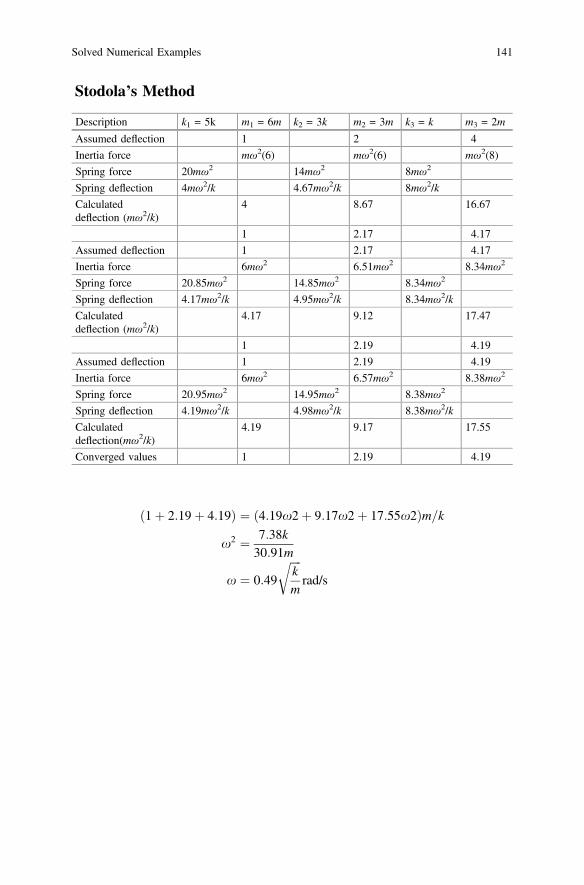
Stodola’s Method
ð1þ 2:19þ 4:19Þ ¼ ð4:19x2þ 9:17x2þ 17:55x2Þm=kx2 ¼ 7:38k
30:91m
x ¼ 0:49
ffiffiffiffikm
rrad/s
Description k1 = 5k m1 = 6m k2 = 3k m2 = 3m k3 = k m3 = 2m
Assumed deflection 1 2 4
Inertia force mω2(6) mω2(6) mω2(8)
Spring force 20mω2 14mω2 8mω2
Spring deflection 4mω2/k 4.67mω2/k 8mω2/k
Calculateddeflection (mω2/k)
4 8.67 16.67
1 2.17 4.17
Assumed deflection 1 2.17 4.17
Inertia force 6mω2 6.51mω2 8.34mω2
Spring force 20.85mω2 14.85mω2 8.34mω2
Spring deflection 4.17mω2/k 4.95mω2/k 8.34mω2/k
Calculateddeflection (mω2/k)
4.17 9.12 17.47
1 2.19 4.19
Assumed deflection 1 2.19 4.19
Inertia force 6mω2 6.57mω2 8.38mω2
Spring force 20.95mω2 14.95mω2 8.38mω2
Spring deflection 4.19mω2/k 4.98mω2/k 8.38mω2/k
Calculateddeflection(mω2/k)
4.19 9.17 17.55
Converged values 1 2.19 4.19
Solved Numerical Examples 141
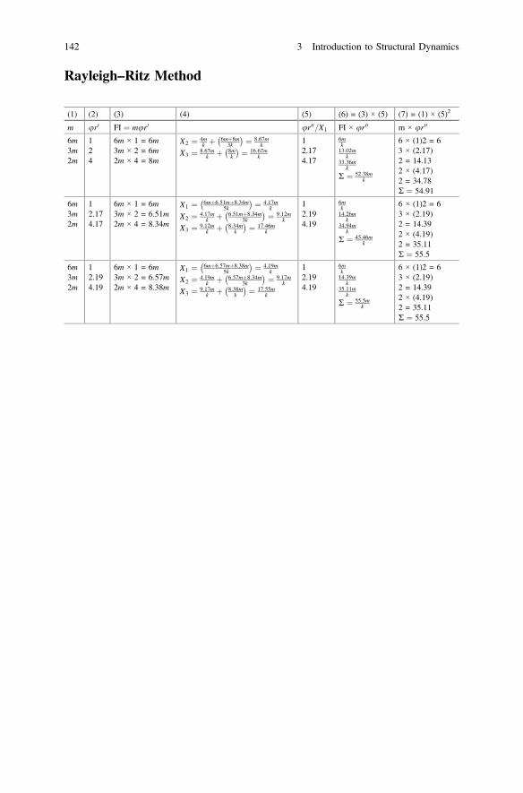
Rayleigh–Ritz Method
(1) (2) (3) (4) (5) (6) = (3) × (5) (7) = (1) × (5)2
m ur0 FI ¼ mur0 ur00=X1 FI × ur00 m × ur00
6m3m2m
124
6m × 1 = 6m3m × 2 = 6m2m × 4 = 8m
X2 ¼ 4mk þ 6mþ8m
3k
� � ¼ 8:67mk
X3 ¼ 8:67mk þ 8m
k
� � ¼ 16:67mk
12.174.17
6mk13:02m
k33:36m
k
R ¼ 52:38mk
6 × (1)2 = 63 × (2.17)2 = 14.132 × (4.17)2 = 34.78R ¼ 54:91
6m3m2m
12.174.17
6m × 1 = 6m3m × 2 = 6.51m2m × 4 = 8.34m
X1 ¼ 6mþ6:51mþ8:34m5k
� � ¼ 4:17mk
X2 ¼ 4:17mk þ 6:51mþ8:34m
3k
� � ¼ 9:12mk
X3 ¼ 9:12mk þ 8:34m
k
� � ¼ 17:46mk
12.194.19
6mk14:26m
k34:94m
k
R ¼ 45:46mk
6 × (1)2 = 63 × (2.19)2 = 14.392 × (4.19)2 = 35.11R ¼ 55:5
6m3m2m
12.194.19
6m × 1 = 6m3m × 2 = 6.57m2m × 4 = 8.38m
X1 ¼ 6mþ6:57mþ8:38m5k
� � ¼ 4:19mk
X2 ¼ 4:19mk þ 6:57mþ8:34m
3k
� � ¼ 9:17mk
X3 ¼ 9:17mk þ 8:38m
k
� � ¼ 17:55mk
12.194.19
6mk14:39m
k35:11m
k
R ¼ 55:5mk
6 × (1)2 = 63 × (2.19)2 = 14.392 × (4.19)2 = 35.11R ¼ 55:5
142 3 Introduction to Structural Dynamics
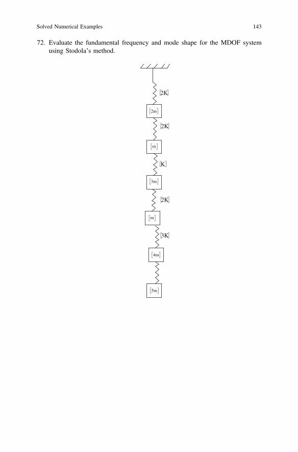
72. Evaluate the fundamental frequency and mode shape for the MDOF systemusing Stodola’s method.
2m
m
3m
2K
2K
K
2K
m
3K
4m
5m
[ ]
[ ]
[ ]
[ ]
[ ]
[ ]
[ ]
[ ]
[ ]
[ ]
[ ]
Solved Numerical Examples 143
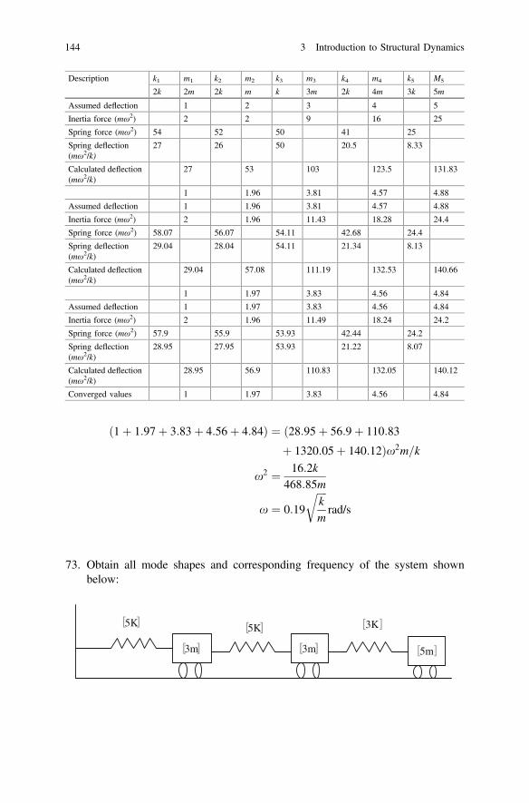
ð1þ 1:97þ 3:83þ 4:56þ 4:84Þ ¼ ð28:95þ 56:9þ 110:83
þ 1320:05þ 140:12Þx2m=k
x2 ¼ 16:2k468:85m
x ¼ 0:19
ffiffiffiffikm
rrad/s
73. Obtain all mode shapes and corresponding frequency of the system shownbelow:
Description k1 m1 k2 m2 k3 m3 k4 m4 k5 M5
2k 2m 2k m k 3m 2k 4m 3k 5m
Assumed deflection 1 2 3 4 5
Inertia force (mω2) 2 2 9 16 25
Spring force (mω2) 54 52 50 41 25
Spring deflection(mω2/k)
27 26 50 20.5 8.33
Calculated deflection(mω2/k)
27 53 103 123.5 131.83
1 1.96 3.81 4.57 4.88
Assumed deflection 1 1.96 3.81 4.57 4.88
Inertia force (mω2) 2 1.96 11.43 18.28 24.4
Spring force (mω2) 58.07 56.07 54.11 42.68 24.4
Spring deflection(mω2/k)
29.04 28.04 54.11 21.34 8.13
Calculated deflection(mω2/k)
29.04 57.08 111.19 132.53 140.66
1 1.97 3.83 4.56 4.84
Assumed deflection 1 1.97 3.83 4.56 4.84
Inertia force (mω2) 2 1.96 11.49 18.24 24.2
Spring force (mω2) 57.9 55.9 53.93 42.44 24.2
Spring deflection(mω2/k)
28.95 27.95 53.93 21.22 8.07
Calculated deflection(mω2/k)
28.95 56.9 110.83 132.05 140.12
Converged values 1 1.97 3.83 4.56 4.84
3m 3m 5m
5K 5K 3K[ ]
[ ]
[ ]
[ ]
[ ]
[ ]
144 3 Introduction to Structural Dynamics
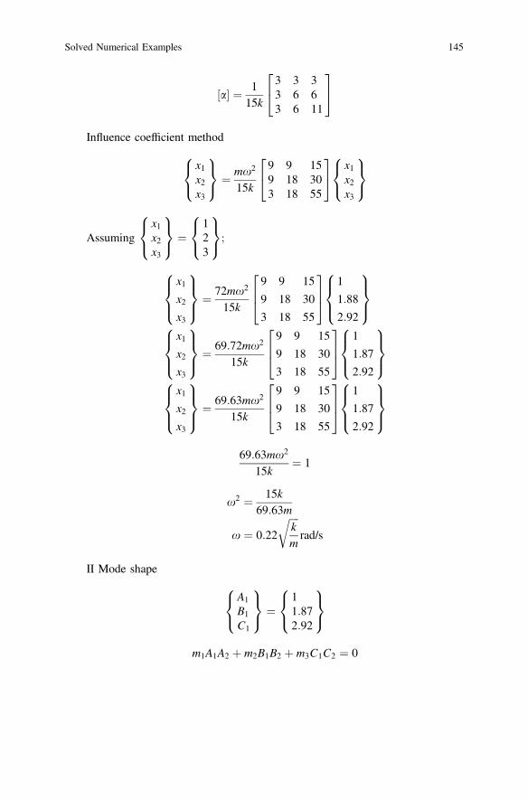
½a� ¼ 115k
3 3 33 6 63 6 11
24
35
Influence coefficient method
x1x2x3
8<:
9=; ¼ mx2
15k
9 9 159 18 303 18 55
24
35 x1
x2x3
8<:
9=;
Assumingx1x2x3
8<:
9=; ¼
123
8<:
9=;;
x1x2x3
8><>:
9>=>; ¼ 72mx2
15k
9 9 15
9 18 30
3 18 55
264
375
1
1:88
2:92
8><>:
9>=>;
x1x2x3
8><>:
9>=>; ¼ 69:72mx2
15k
9 9 15
9 18 30
3 18 55
264
375
1
1:87
2:92
8><>:
9>=>;
x1x2x3
8><>:
9>=>; ¼ 69:63mx2
15k
9 9 15
9 18 30
3 18 55
264
375
1
1:87
2:92
8><>:
9>=>;
69:63mx2
15k¼ 1
x2 ¼ 15k69:63m
x ¼ 0:22
ffiffiffiffikm
rrad/s
II Mode shape
A1
B1
C1
8<:
9=; ¼
11:872:92
8<:
9=;
m1A1A2 þ m2B1B2 þ m3C1C2 ¼ 0
Solved Numerical Examples 145
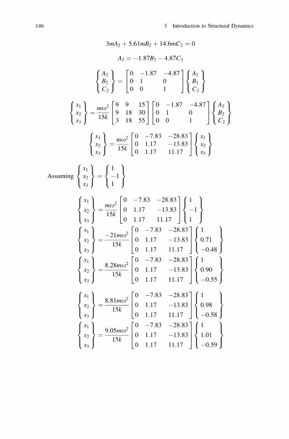
3mA2 þ 5:61mB2 þ 14:6mC2 ¼ 0
A2 ¼ �1:87B2 � 4:87C2
A2
B2
C2
8<:
9=; ¼
0 �1:87 �4:870 1 00 0 1
24
35 A2
B2
C2
8<:
9=;
x1x2x3
8<:
9=; ¼ mx2
15k
9 9 159 18 303 18 55
24
35 0 �1:87 �4:87
0 1 00 0 1
24
35 A2
B2
C2
8<:
9=;
x1x2x3
8<:
9=; ¼ mx2
15k
0 �7:83 �28:830 1:17 �13:830 1:17 11:17
24
35 x1
x2x3
8<:
9=;
Assumingx1x2x3
8<:
9=; ¼
1�11
8<:
9=;
x1x2x3
8><>:
9>=>; ¼ mx2
15k
0 �7:83 �28:83
0 1:17 �13:83
0 1:17 11:17
264
375
1
�1
1
8><>:
9>=>;
x1x2x3
8><>:
9>=>; ¼ �21mx2
15k
0 �7:83 �28:83
0 1:17 �13:83
0 1:17 11:17
264
375
1
0:71
�0:48
8><>:
9>=>;
x1x2x3
8><>:
9>=>; ¼ 8:28mx2
15k
0 �7:83 �28:83
0 1:17 �13:83
0 1:17 11:17
264
375
1
0:90
�0:55
8><>:
9>=>;
x1x2x3
8><>:
9>=>; ¼ 8:81mx2
15k
0 �7:83 �28:83
0 1:17 �13:83
0 1:17 11:17
264
375
1
0:98
�0:58
8><>:
9>=>;
x1x2x3
8><>:
9>=>; ¼ 9:05mx2
15k
0 �7:83 �28:83
0 1:17 �13:83
0 1:17 11:17
264
375
1
1:01
�0:59
8><>:
9>=>;
146 3 Introduction to Structural Dynamics
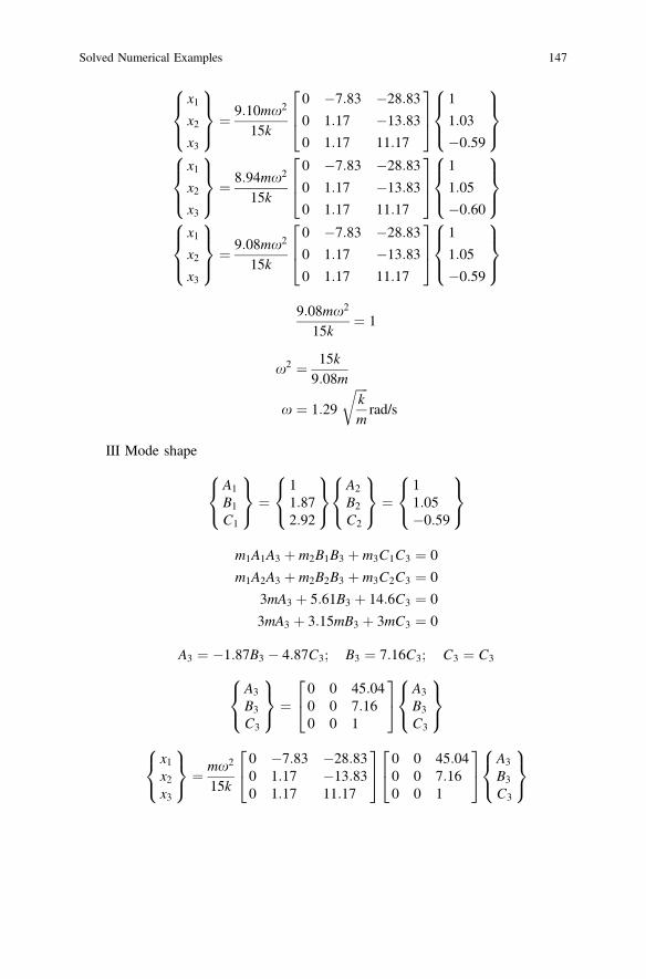
x1x2x3
8><>:
9>=>; ¼ 9:10mx2
15k
0 �7:83 �28:83
0 1:17 �13:83
0 1:17 11:17
264
375
1
1:03
�0:59
8><>:
9>=>;
x1x2x3
8><>:
9>=>; ¼ 8:94mx2
15k
0 �7:83 �28:83
0 1:17 �13:83
0 1:17 11:17
264
375
1
1:05
�0:60
8><>:
9>=>;
x1x2x3
8><>:
9>=>; ¼ 9:08mx2
15k
0 �7:83 �28:83
0 1:17 �13:83
0 1:17 11:17
264
375
1
1:05
�0:59
8><>:
9>=>;
9:08mx2
15k¼ 1
x2 ¼ 15k9:08m
x ¼ 1:29
ffiffiffiffikm
rrad/s
III Mode shape
A1
B1
C1
8<:
9=; ¼
11:872:92
8<:
9=;
A2
B2
C2
8<:
9=; ¼
11:05�0:59
8<:
9=;
m1A1A3 þ m2B1B3 þ m3C1C3 ¼ 0
m1A2A3 þ m2B2B3 þ m3C2C3 ¼ 0
3mA3 þ 5:61B3 þ 14:6C3 ¼ 0
3mA3 þ 3:15mB3 þ 3mC3 ¼ 0
A3 ¼ �1:87B3 � 4:87C3; B3 ¼ 7:16C3; C3 ¼ C3
A3
B3
C3
8<:
9=; ¼
0 0 45:040 0 7:160 0 1
24
35 A3
B3
C3
8<:
9=;
x1x2x3
8<:
9=; ¼ mx2
15k
0 �7:83 �28:830 1:17 �13:830 1:17 11:17
24
35 0 0 45:04
0 0 7:160 0 1
24
35 A3
B3
C3
8<:
9=;
Solved Numerical Examples 147
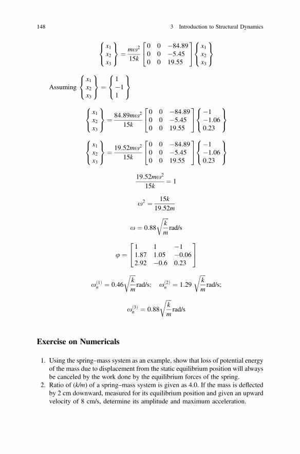
x1x2x3
8<:
9=; ¼ mx2
15k
0 0 �84:890 0 �5:450 0 19:55
24
35 x1
x2x3
8<:
9=;
Assumingx1x2x3
8<:
9=; ¼
1�11
8<:
9=;
x1x2x3
8<:
9=; ¼ 84:89mx2
15k
0 0 �84:890 0 �5:450 0 19:55
24
35 �1
�1:060:23
8<:
9=;
x1x2x3
8<:
9=; ¼ 19:52mx2
15k
0 0 �84:890 0 �5:450 0 19:55
24
35 �1
�1:060:23
8<:
9=;
19:52mx2
15k¼ 1
x2 ¼ 15k19:52m
x ¼ 0:88
ffiffiffiffikm
rrad/s
u ¼1 1 �11:87 1:05 �0:062:92 �0:6 0:23
24
35
xð1Þn ¼ 0:46
ffiffiffiffikm
rrad/s; xð2Þ
n ¼ 1:29
ffiffiffiffikm
rrad/s;
xð3Þn ¼ 0:88
ffiffiffiffikm
rrad/s
Exercise on Numericals
1. Using the spring–mass system as an example, show that loss of potential energyof the mass due to displacement from the static equilibrium position will alwaysbe canceled by the work done by the equilibrium forces of the spring.
2. Ratio of (k/m) of a spring–mass system is given as 4.0. If the mass is deflectedby 2 cm downward, measured for its equilibrium position and given an upwardvelocity of 8 cm/s, determine its amplitude and maximum acceleration.
148 3 Introduction to Structural Dynamics
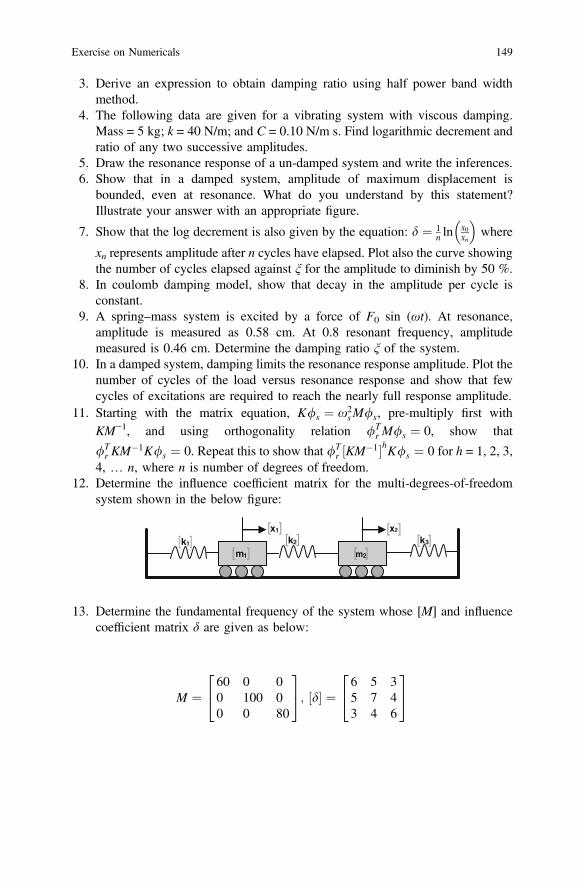
3. Derive an expression to obtain damping ratio using half power band widthmethod.
4. The following data are given for a vibrating system with viscous damping.Mass = 5 kg; k = 40 N/m; and C = 0.10 N/m s. Find logarithmic decrement andratio of any two successive amplitudes.
5. Draw the resonance response of a un-damped system and write the inferences.6. Show that in a damped system, amplitude of maximum displacement is
bounded, even at resonance. What do you understand by this statement?Illustrate your answer with an appropriate figure.
7. Show that the log decrement is also given by the equation: d ¼ 1n ln
x0xn
� �where
xn represents amplitude after n cycles have elapsed. Plot also the curve showingthe number of cycles elapsed against ξ for the amplitude to diminish by 50 %.
8. In coulomb damping model, show that decay in the amplitude per cycle isconstant.
9. A spring–mass system is excited by a force of F0 sin (ωt). At resonance,amplitude is measured as 0.58 cm. At 0.8 resonant frequency, amplitudemeasured is 0.46 cm. Determine the damping ratio ξ of the system.
10. In a damped system, damping limits the resonance response amplitude. Plot thenumber of cycles of the load versus resonance response and show that fewcycles of excitations are required to reach the nearly full response amplitude.
11. Starting with the matrix equation, K/s ¼ x2sM/s, pre-multiply first with
KM−1, and using orthogonality relation /Tr M/s ¼ 0, show that
/Tr KM
�1K/s ¼ 0. Repeat this to show that /Tr KM�1½ �hK/s ¼ 0 for h = 1, 2, 3,
4, … n, where n is number of degrees of freedom.12. Determine the influence coefficient matrix for the multi-degrees-of-freedom
system shown in the below figure:
k1 k2 k3
m1 m2
x2x1
[ ][ ]
[ ][ ]
[ ]
[ ][ ]
13. Determine the fundamental frequency of the system whose [M] and influencecoefficient matrix δ are given as below:
M ¼60 0 00 100 00 0 80
24
35; ½d� ¼ 6 5 3
5 7 43 4 6
24
35
Exercise on Numericals 149

14. What do you understand by mode shapes? Give its physical interpretation.15. Why fundamental frequency is of great importance in structural dynamics?16. A continuous structure has ________ number of degrees of freedom.17. In structural dynamics, mass element represents ______ characteristics of the
structure and _______ represents elastic restoring force.18. A sketch of the body, isolated from all other bodies, in which all forces external
to the body are shown is called _______.19. An alternate approach which states that the system may be set in a state of
dynamic equilibrium is called __________.20. Degree of freedom of a system is the number of independent coordinates
necessary to describe its position. True or false. If false, rewrite the correctstatement.
21. It is observed experimentally that amplitude of free vibration of certainstructure modeled as single degree of freedom decreases from 1 to 0.4 in 10cycles. What is the % of critical damping?
22. The simplest form of periodic motion is ________.23. What are the essential characteristics of a dynamic loading?24. It is not always possible to obtain rigorous mathematical solutions for engi-
neering problems. Should you agree to this statement, then which provides areasonable link between the real physical system and mathematically feasiblesolution?
25. It is not always of freedom, damping element represents only dissipation ofenergy. Such pure elements do not exist in physical world this statement, thenwhich provides a ra mathematical model.
26. Do both the figures shown below represent mathematical models that aredynamically equivalent? Explain your answer briefly.
27. In a SDOF model, spring is considered a linear spring. In other words, force–displacement properties of the system are taken as linear. Is it a hypotheticalsituation compared to the real dynamic behavior of structures? Explain.
28. Find time period of the structure shown in the below figure. Cross section ofthe column is circular of 50 mm diameter, made of steel. Take Est as 2 × 10⁵ N/mm2, mass as 100 kg, length of the column as 2 m.
150 3 Introduction to Structural Dynamics
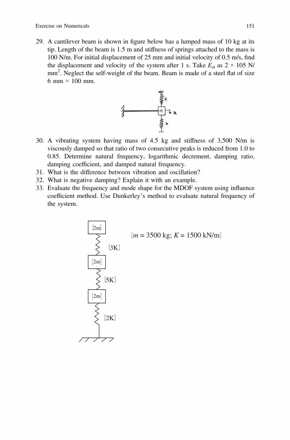
29. A cantilever beam is shown in figure below has a lumped mass of 10 kg at itstip. Length of the beam is 1.5 m and stiffness of springs attached to the mass is100 N/m. For initial displacement of 25 mm and initial velocity of 0.5 m/s, findthe displacement and velocity of the system after 1 s. Take Est as 2 × 10⁵ N/mm2. Neglect the self-weight of the beam. Beam is made of a steel flat of size6 mm × 100 mm.
30. A vibrating system having mass of 4.5 kg and stiffness of 3,500 N/m isviscously damped so that ratio of two consecutive peaks is reduced from 1.0 to0.85. Determine natural frequency, logarithmic decrement, damping ratio,damping coefficient, and damped natural frequency.
31. What is the difference between vibration and oscillation?32. What is negative damping? Explain it with an example.33. Evaluate the frequency and mode shape for the MDOF system using influence
coefficient method. Use Dunkerley’s method to evaluate natural frequency ofthe system.
2m
2m
2m
2K
3K
5K
m = 3500 kg; K = 1500 kN/m[ ]
[ ]
[ ]
[ ]
[ ]
[ ]
[ ]
Exercise on Numericals 151
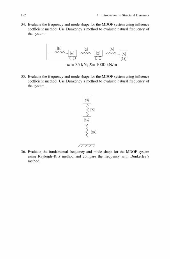
34. Evaluate the frequency and mode shape for the MDOF system using influencecoefficient method. Use Dunkerley’s method to evaluate natural frequency ofthe system.
m 2 5
K 2 K[ ][ ]
[ ][ ]
[ ][ ]
m = 35 kN; K= 1000 kN/m
35. Evaluate the frequency and mode shape for the MDOF system using influencecoefficient method. Use Dunkerley’s method to evaluate natural frequency ofthe system.
5m
2m
2K
K
[ ]
[ ]
[ ]
[ ]
36. Evaluate the fundamental frequency and mode shape for the MDOF systemusing Rayleigh–Ritz method and compare the frequency with Dunkerley’smethod.
152 3 Introduction to Structural Dynamics
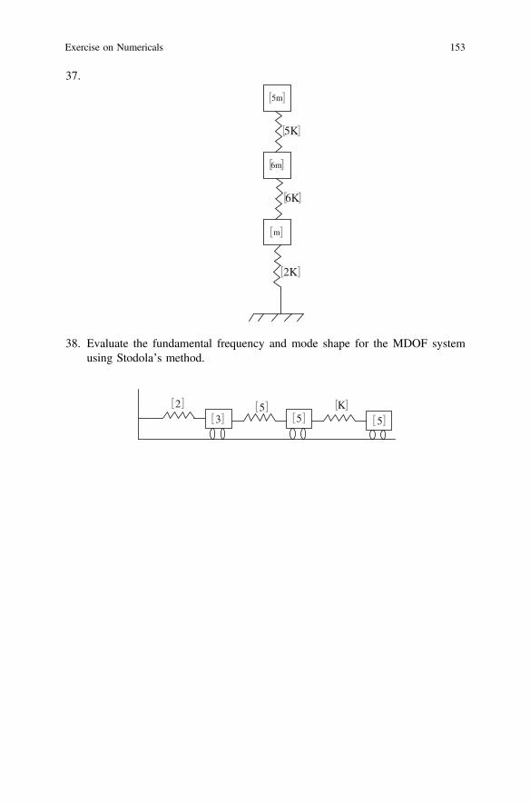
37.
5m
6m
m
2K
5K
6K
[ ]
[ ]
[ ]
[ ]
[ ]
[ ]
38. Evaluate the fundamental frequency and mode shape for the MDOF systemusing Stodola’s method.
3 5 5
2 5 K[ ][ ]
[ ][ ]
[ ][ ]
Exercise on Numericals 153
Chapter 4Damping in Offshore Structures
Abstract This chapter deals with the methods of estimating damping in offshorestructures. Different types of damping models, their comparison, and suitability tooffshore structures are discussed in detail. Example problems are solved, andestimation of damping using different models is explained.
Keywords Structural damping � Viscous damping � Coulomb damping � Rayleighdamping � Caughey damping
4.1 Introduction
Under ideal conditions of no damping, if the system is set to vibration, it will beexcited indefinitely at constant amplitude at its natural frequency. But in real time,any system set to vibration comes to rest, necessarily after passage of time; dampingoffered by the presence of air may be one of the reasons. As such, un-dampedsystems are hypothetical, since damping is inherently present in the atmosphere.Further, ocean structures are under the influence of waves and current, which offerssignificant amount of damping to the structural system that is set in vibration. Thebasic types of damping are, namely (i) coulomb damping and (ii) viscous damping.Coulomb damping results from sliding of two surfaces; it is also called dry dampingor friction damping. The damping force is the product of the normal force and thecoefficient of friction between the body surface and the plane of motion. Note thatthe damping force in this case is independent of velocity of motion of the bodywhich is under vibration. In case of viscous damping, the damping force accountsfor the viscosity of the system. The presence of fluid medium around the bodysignificantly influences the damping force acting on the body. Damping force willbe proportional to the magnitude of the velocity and has the unit of N/(m s).Viscous damping seems to be more relevant to offshore structural systems due tothe inherent presence of liquid medium around the body.
© Springer India 2015S. Chandrasekaran, Dynamic Analysis and Design of Offshore Structures,Ocean Engineering & Oceanography 5, DOI 10.1007/978-81-322-2277-4_4
155
The frictional forces are not conservative, as they cannot be derived from apotential function that is based on the displacement (response) of the vibratingsystem. However, these forces are highly responsible for dissipation of energy orconversion of energy from one form to the other. This results in reduction inresponse to the structural system. The energy consumed by the friction forces isconverted into heat energy and dissipated by conduction, by convection to the fluidsurrounding the structure and by radiation.
The frictional forces in a system may arise due to any one of the followingphysical processes (Wilson 1984). There can be friction among the materials,leading to internal viscous damping. This is highly practical due to the use of modernmaterials such as composites in offshore structures. At the connections or joints, dueto the presence of materials of different composition, bimetallic coupling can resultin friction forces. There can also be friction between two structural components,leading to structural damping. There can be friction between the structural membersand fluid surrounding them, leading to external viscous damping. Lastly, there canbe friction between the structural members at their supports which are in contact withthem. This leads to coulomb damping. However, it is very difficult to quantify thesedamping forces in a given system, as the causes for such forces are diverse.
Structural damping is usually considered to be 0.2–0.5 % of that of the criticaldamping for steel platforms (Adams and Baltrop 1991). For concrete, this can be ofthe order of 0.5–1.5 %. Hydrodynamic damping originates from the waves sur-rounding the offshore structures. They are found in two common forms, namely (i)radiation damping and (ii) viscous damping. Radiation damping is determined bypotential theory. It exhibits a strong dependence on frequency and submergenceeffects. Literature shows that the drag damping is lower for a larger diametervertical column members in offshore structures; this is of the order 0.1 %. Dampingratio of the marine structure, including the effect of added mass can be expressed asthe ratio of the dry structure, as given below:
nwet ¼ ndrym�
dryx�dry
m�wetx
�wet
� �ð4:1Þ
where m* and x� are generalized mass and frequency, respectively (Naess andMoan 2013). Literature also shows that the total damping ratio is about 2 % for thefirst three modes for gravity platforms.
Classical damping is an approximate idealization if similar damping is distrib-uted throughout the structure. However, in offshore structures, uniform distributionof damping throughout the structure is not applicable due to many reasons:(i) variation in material properties of members at connections, (ii) use of compositesfor variety of members, and (iii) deck and the substructure shall be even isolated sothat the large displacements of the deck under wind forces do not influence the
156 4 Damping in Offshore Structures
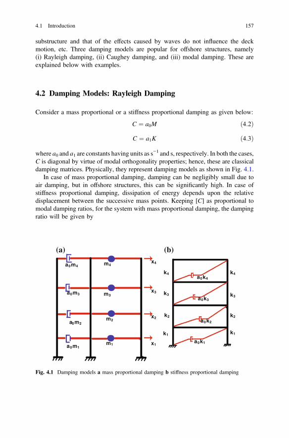
substructure and that of the effects caused by waves do not influence the deckmotion, etc. Three damping models are popular for offshore structures, namely(i) Rayleigh damping, (ii) Caughey damping, and (iii) modal damping. These areexplained below with examples.
4.2 Damping Models: Rayleigh Damping
Consider a mass proportional or a stiffness proportional damping as given below:
C ¼ a0M ð4:2Þ
C ¼ a1K ð4:3Þ
where a0 and a1 are constants having units as s−1 and s, respectively. In both the cases,
C is diagonal by virtue of modal orthogonality properties; hence, these are classicaldamping matrices. Physically, they represent damping models as shown in Fig. 4.1.
In case of mass proportional damping, damping can be negligibly small due toair damping, but in offshore structures, this can be significantly high. In case ofstiffness proportional damping, dissipation of energy depends upon the relativedisplacement between the successive mass points. Keeping [C] as proportional tomodal damping ratios, for the system with mass proportional damping, the dampingratio will be given by
m1
m2
m3
m4x4
x3
x2
x1a0m1
a0m2
a0m3
a0m4
a0k1
a0k2
a0k3
a0k4
k1
k2
k3
k4
k1
k2
k3
k4
(a) (b)
Fig. 4.1 Damping models a mass proportional damping b stiffness proportional damping
4.1 Introduction 157
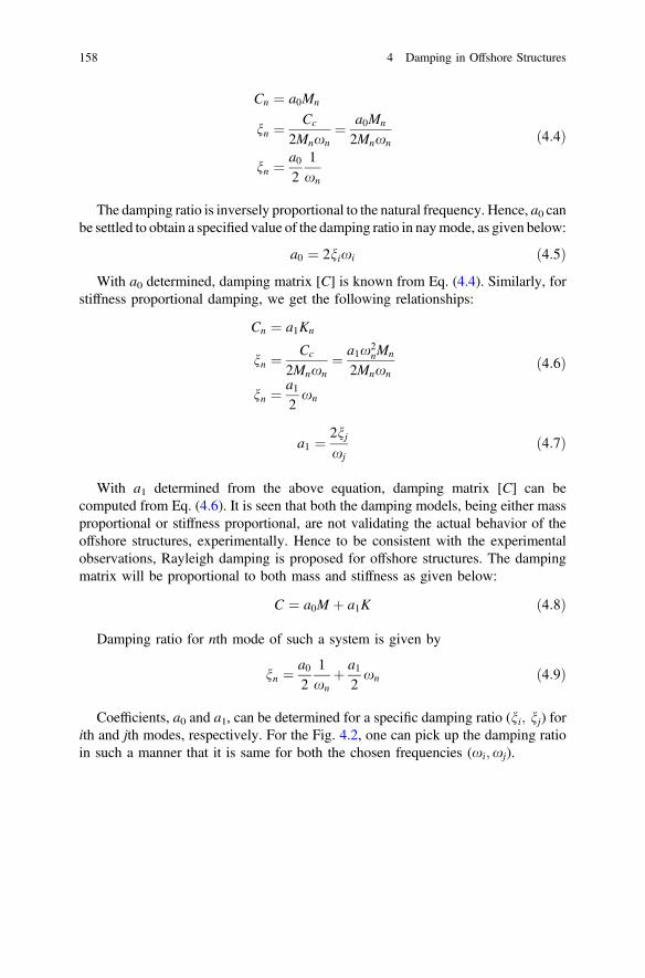
Cn ¼ a0Mn
nn ¼Cc
2Mnxn¼ a0Mn
2Mnxn
nn ¼a02
1xn
ð4:4Þ
The damping ratio is inversely proportional to the natural frequency. Hence, a0 canbe settled to obtain a specified value of the damping ratio in naymode, as given below:
a0 ¼ 2nixi ð4:5ÞWith a0 determined, damping matrix [C] is known from Eq. (4.4). Similarly, for
stiffness proportional damping, we get the following relationships:
Cn ¼ a1Kn
nn ¼Cc
2Mnxn¼ a1x2
nMn
2Mnxn
nn ¼a12xn
ð4:6Þ
a1 ¼2njxj
ð4:7Þ
With a1 determined from the above equation, damping matrix [C] can becomputed from Eq. (4.6). It is seen that both the damping models, being either massproportional or stiffness proportional, are not validating the actual behavior of theoffshore structures, experimentally. Hence to be consistent with the experimentalobservations, Rayleigh damping is proposed for offshore structures. The dampingmatrix will be proportional to both mass and stiffness as given below:
C ¼ a0M þ a1K ð4:8Þ
Damping ratio for nth mode of such a system is given by
nn ¼a02
1xn
þ a12xn ð4:9Þ
Coefficients, a0 and a1, can be determined for a specific damping ratio (ni; nj) forith and jth modes, respectively. For the Fig. 4.2, one can pick up the damping ratioin such a manner that it is same for both the chosen frequencies (xi;xj).
158 4 Damping in Offshore Structures
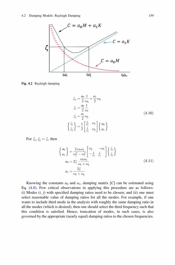
nn ¼a02
1xn
þ a12xn
ni ¼a02
1xi
nj ¼a12xj
ninj
� �¼ 1
2
1xi
xi
1xj
xj
" #a0a1
� �ð4:10Þ
For ni; nj ¼ n, then
a0a1
� �¼ 2xixj
x2j � x2
i
xj �xi
� 1xj
1xi
" #ninj
� �
a0 ¼ 2nxixj
xi þ xj
a1 ¼ 2nxi þ xj
ð4:11Þ
Knowing the constants a0 and a1, damping matrix [C] can be estimated usingEq. (4.8). Few critical observations in applying this procedure are as follows:(i) Modes (i, j) with specified damping ratios need to be chosen; and (ii) one mustselect reasonable value of damping ratios for all the modes. For example, if onewants to include third mode in the analysis with roughly the same damping ratio inall the modes (which is desired), then one should select the third frequency such thatthis condition is satisfied. Hence, truncation of modes, in such cases, is alsogoverned by the appropriate (nearly equal) damping ratios to the chosen frequencies.
Fig. 4.2 Rayleigh damping
4.2 Damping Models: Rayleigh Damping 159
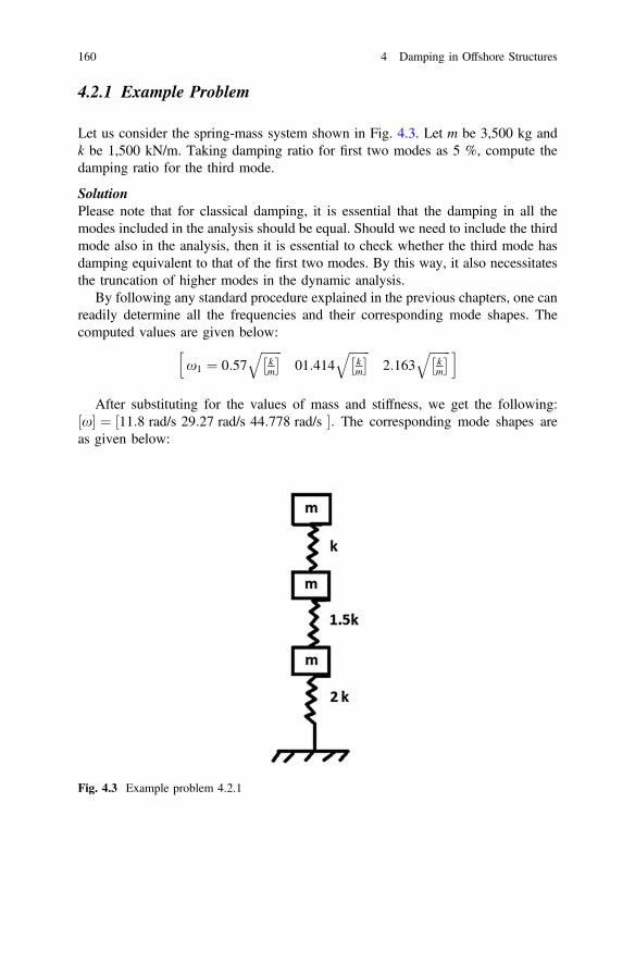
4.2.1 Example Problem
Let us consider the spring-mass system shown in Fig. 4.3. Let m be 3,500 kg andk be 1,500 kN/m. Taking damping ratio for first two modes as 5 %, compute thedamping ratio for the third mode.
SolutionPlease note that for classical damping, it is essential that the damping in all themodes included in the analysis should be equal. Should we need to include the thirdmode also in the analysis, then it is essential to check whether the third mode hasdamping equivalent to that of the first two modes. By this way, it also necessitatesthe truncation of higher modes in the dynamic analysis.
By following any standard procedure explained in the previous chapters, one canreadily determine all the frequencies and their corresponding mode shapes. Thecomputed values are given below:
x1 ¼ 0:57ffiffiffiffiffiffiffikm
� �q01:414
ffiffiffiffiffiffiffikm
� �q2:163
ffiffiffiffiffiffiffikm
� �qh i
After substituting for the values of mass and stiffness, we get the following:x½ � ¼ 11:8 rad/s 29:27 rad/s 44:778 rad/s½ �: The corresponding mode shapes areas given below:
Fig. 4.3 Example problem 4.2.1
160 4 Damping in Offshore Structures
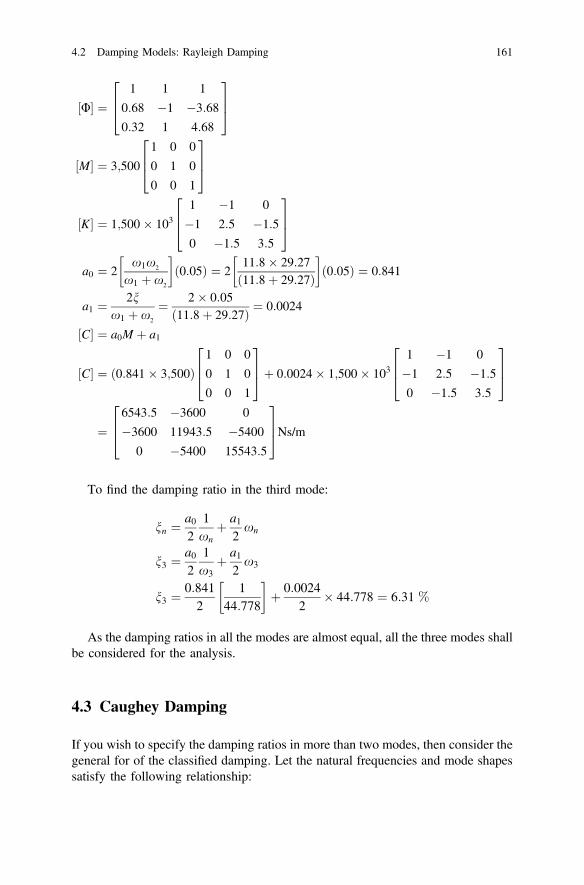
U½ � ¼1 1 1
0:68 �1 �3:68
0:32 1 4:68
264
375
M½ � ¼ 3;500
1 0 0
0 1 0
0 0 1
264
375
K½ � ¼ 1;500� 1031 �1 0
�1 2:5 �1:5
0 �1:5 3:5
264
375
a0 ¼ 2x1x2
x1 þ x2
� �ð0:05Þ ¼ 2
11:8� 29:27ð11:8þ 29:27Þ
� �ð0:05Þ ¼ 0:841
a1 ¼ 2nx1 þ x2
¼ 2� 0:05ð11:8þ 29:27Þ ¼ 0:0024
½C� ¼ a0M þ a1
½C� ¼ ð0:841� 3;500Þ1 0 0
0 1 0
0 0 1
264
375þ 0:0024� 1;500� 103
1 �1 0
�1 2:5 �1:5
0 �1:5 3:5
264
375
¼6543:5 �3600 0
�3600 11943:5 �5400
0 �5400 15543:5
264
375Ns/m
To find the damping ratio in the third mode:
nn ¼a02
1xn
þ a12xn
n3 ¼a02
1x3
þ a12x3
n3 ¼0:8412
144:778
� �þ 0:0024
2� 44:778 ¼ 6:31 %
As the damping ratios in all the modes are almost equal, all the three modes shallbe considered for the analysis.
4.3 Caughey Damping
If you wish to specify the damping ratios in more than two modes, then consider thegeneral for of the classified damping. Let the natural frequencies and mode shapessatisfy the following relationship:
4.2 Damping Models: Rayleigh Damping 161
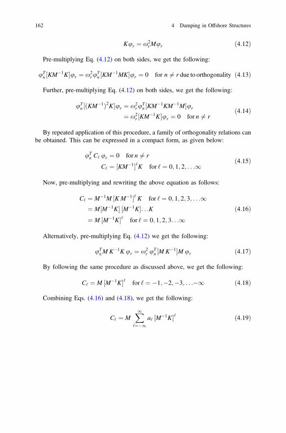
Kur ¼ x2rMur ð4:12Þ
Pre-multiplying Eq. (4.12) on both sides, we get the following:
uTn ½KM�1K�ur ¼ x2
ruTn ½KM�1MK�ur ¼ 0 for n 6¼ r due to orthogonality ð4:13Þ
Further, pre-multiplying Eq. (4.12) on both sides, we get the following:
uTn ½ðKM�1Þ2K�ur ¼ x2
ruTn ½KM�1KM�1M�ur
¼ x2r ½KM�1K�ur ¼ 0 for n 6¼ r
ð4:14Þ
By repeated application of this procedure, a family of orthogonality relations canbe obtained. This can be expressed in a compact form, as given below:
uTn C‘ ur ¼ 0 for n 6¼ r
C‘ ¼ ½KM�1�‘K for ‘ ¼ 0; 1; 2; . . .1ð4:15Þ
Now, pre-multiplying and rewriting the above equation as follows:
C‘ ¼ M�1M ½K M�1�‘ K for ‘ ¼ 0; 1; 2; 3; . . .1¼ M½M�1K� ½M�1K�. . .K¼ M ½M�1K�‘ for ‘ ¼ 0; 1; 2; 3. . .1
ð4:16Þ
Alternatively, pre-multiplying Eq. (4.12) we get the following:
uTnM K�1K ur ¼ x2
r uTn ½MK�1�M ur ð4:17Þ
By following the same procedure as discussed above, we get the following:
C‘ ¼ M ½M�1K�‘ for ‘ ¼ �1;�2;�3; . . .�1 ð4:18Þ
Combining Eqs. (4.16) and (4.18), we get the following:
C‘ ¼ MX1‘¼�1
a‘ ½M�1K�‘ ð4:19Þ
162 4 Damping in Offshore Structures
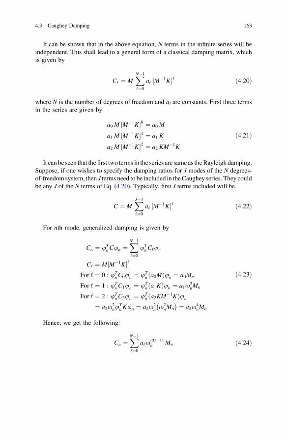
It can be shown that in the above equation, N terms in the infinite series will beindependent. This shall lead to a general form of a classical damping matrix, whichis given by
C‘ ¼ MXN�1
‘¼0
a‘ ½M�1K�‘ ð4:20Þ
where N is the number of degrees of freedom and al are constants. First three termsin the series are given by
a0 M ½M�1K�0 ¼ a0 M
a1 M ½M�1K�1 ¼ a1 K
a2 M ½M�1K�2 ¼ a2 KM�1K
ð4:21Þ
It can be seen that thefirst two terms in the series are same as theRayleigh damping.Suppose, if one wishes to specify the damping ratios for J modes of the N degrees-of-freedom system, then J terms need to be included in theCaughey series. They couldbe any J of the N terms of Eq. (4.20). Typically, first J terms included will be
C ¼ MXJ�1
‘¼0
a‘ ½M�1K�‘ ð4:22Þ
For nth mode, generalized damping is given by
Cn ¼ uTnCun ¼
XN�1
‘¼0
uTnC‘un
C‘ ¼ M½M�1K�‘For ‘ ¼ 0 : uT
nC0un ¼ uTn ða0MÞun ¼ a0Mn
For ‘ ¼ 1 : uTnC1un ¼ uT
n ða1KÞun ¼ a1x2nMn
For ‘ ¼ 2 : uTnC2un ¼ uT
n ða2KM�1KÞun
¼ a2x2nu
TnKun ¼ a2x
2n x2
nMn ¼ a2x
4nMn
ð4:23Þ
Hence, we get the following:
Cn ¼XN�1
‘¼0
a‘xð2‘�1Þn Mn ð4:24Þ
4.3 Caughey Damping 163
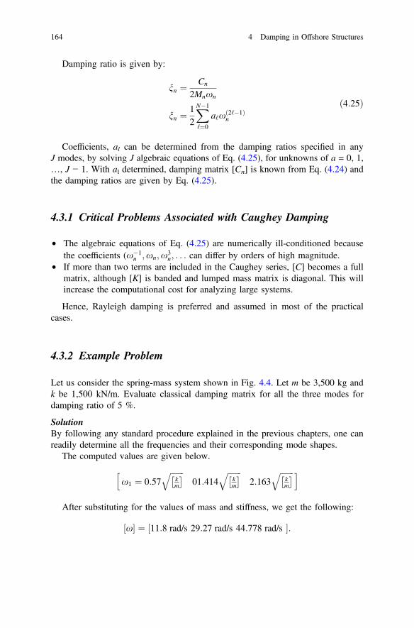
Damping ratio is given by:
nn ¼Cn
2Mnxn
nn ¼12
XN�1
‘¼0
a‘xð2‘�1Þn
ð4:25Þ
Coefficients, al can be determined from the damping ratios specified in anyJ modes, by solving J algebraic equations of Eq. (4.25), for unknowns of a = 0, 1,…, J − 1. With al determined, damping matrix [Cn] is known from Eq. (4.24) andthe damping ratios are given by Eq. (4.25).
4.3.1 Critical Problems Associated with Caughey Damping
• The algebraic equations of Eq. (4.25) are numerically ill-conditioned becausethe coefficients (x�1
n ;xn;x3n; . . . can differ by orders of high magnitude.
• If more than two terms are included in the Caughey series, [C] becomes a fullmatrix, although [K] is banded and lumped mass matrix is diagonal. This willincrease the computational cost for analyzing large systems.
Hence, Rayleigh damping is preferred and assumed in most of the practicalcases.
4.3.2 Example Problem
Let us consider the spring-mass system shown in Fig. 4.4. Let m be 3,500 kg andk be 1,500 kN/m. Evaluate classical damping matrix for all the three modes fordamping ratio of 5 %.
SolutionBy following any standard procedure explained in the previous chapters, one canreadily determine all the frequencies and their corresponding mode shapes.
The computed values are given below.
x1 ¼ 0:57ffiffiffiffiffiffiffikm
� �q01:414
ffiffiffiffiffiffiffikm
� �q2:163
ffiffiffiffiffiffiffikm
� �qh i
After substituting for the values of mass and stiffness, we get the following:
x½ � ¼ 11:8 rad/s 29:27 rad/s 44:778 rad/s½ �:
164 4 Damping in Offshore Structures
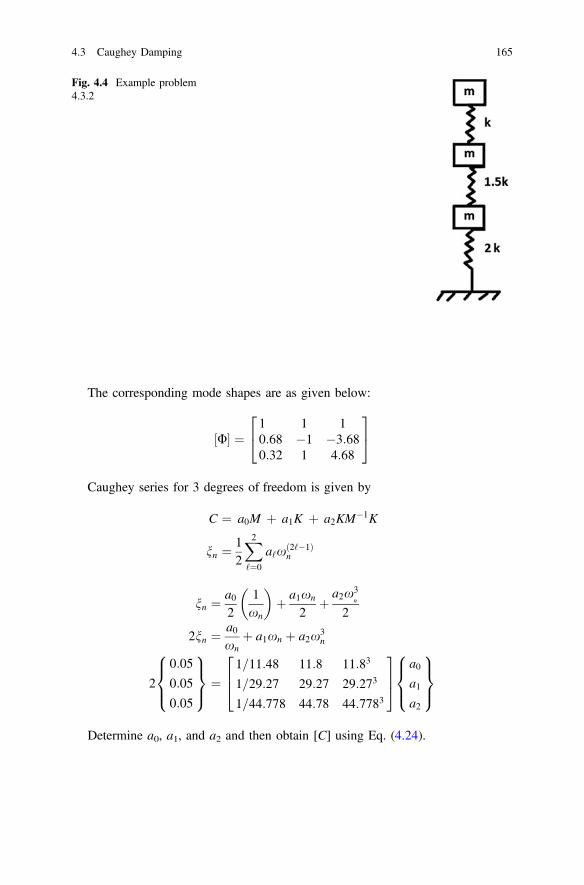
The corresponding mode shapes are as given below:
U½ � ¼1 1 10:68 �1 �3:680:32 1 4:68
24
35
Caughey series for 3 degrees of freedom is given by
C ¼ a0M þ a1K þ a2KM�1K
nn ¼12
X2‘¼0
a‘xð2‘�1Þn
nn ¼a02
1xn
� �þ a1xn
2þ a2x3
n
2
2nn ¼a0xn
þ a1xn þ a2x3n
2
0:05
0:05
0:05
8><>:
9>=>; ¼
1=11:48 11:8 11:83
1=29:27 29:27 29:273
1=44:778 44:78 44:7783
264
375
a0a1a2
8><>:
9>=>;
Determine a0, a1, and a2 and then obtain [C] using Eq. (4.24).
Fig. 4.4 Example problem4.3.2
4.3 Caughey Damping 165
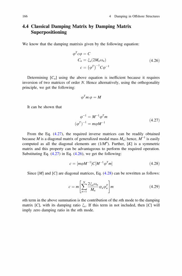
4.4 Classical Damping Matrix by Damping MatrixSuperpositioning
We know that the damping matrixis given by the following equation:
uTcu ¼ C
Cn ¼ nnð2MnxnÞc ¼ uT
�1Cu�1
ð4:26Þ
Determining [Cn] using the above equation is inefficient because it requiresinversion of two matrices of order N. Hence alternatively, using the orthogonalityprinciple, we get the following:
uTmu ¼ M
It can be shown that
u�1 ¼ M�1uTm
ðuTÞ�1 ¼ muM�1ð4:27Þ
From the Eq. (4.27), the required inverse matrices can be readily obtainedbecause M is a diagonal matrix of generalized modal mass Mn; hence, M
−1 is easilycomputed as all the diagonal elements are (1/Mn). Further, [K] is a symmetricmatrix and this property can be advantageous to perform the required operation.Substituting Eq. (4.27) in Eq. (4.26), we get the following:
c ¼ ½muM�1�C½M�1uTm� ð4:28Þ
Since [M] and [C] are diagonal matrices, Eq. (4.28) can be rewritten as follows:
c ¼ mXNn¼1
2nnxn
Mnunu
Tn
" #m ð4:29Þ
nth term in the above summation is the contribution of the nth mode to the dampingmatrix [C], with its damping ratio nn. If this term in not included, then [C] willimply zero damping ratio in the nth mode.
166 4 Damping in Offshore Structures
4.4.1 Critical Issues
• It is practical to include any first J modes even though N degrees of freedomexist.
• Lack of damping in modes (J + 1) to N does not create any numerical problemsin an unconditionally stable time-stepping procedure is chosen to integrate theequation of motion.
4.4.2 Example Problem
Let us consider the spring-mass system shown in Fig. 4.5. Let m be 3,500 kg andk be 1,500 kN/m. Determine damping matrix by superimposing the dampingmatrices for first two modes, each with 5 % damping ratio.
SolutionBy following any standard procedure explained in the previous chapters, one canreadily determine all the frequencies and their corresponding mode shapes.
The computed values are given below.
x1 ¼ 0:57ffiffiffiffiffiffiffikm
� �q01:414
ffiffiffiffiffiffiffikm
� �q2:163
ffiffiffiffiffiffiffikm
� �qh i
After substituting for the values of mass and stiffness, we get the following:
x½ � ¼ 11:8 rad/s 29:27 rad/s 44:778 rad/s½ �:
Fig. 4.5 Example problem4.4.2
4.4 Classical Damping Matrix by Damping Matrix Superpositioning 167
The corresponding mode shapes are as given below:
U½ � ¼1 1 1
0:68 �1 �3:680:32 1 4:68
24
35
The damping matrix is given by Eq. (4.29). Individual term of the matrix is nowdetermined as below:
c1 ¼ 2ð0:05Þð11:8Þ1:0
mu1uT1m
¼ 2ð0:05Þð11:8Þ1:0
ð3;500Þ1 0 0
0 1 0
0 0 1
264
375
1
0:68
0:32
8><>:
9>=>; 1 0:68 0:32½ �ð3;500Þ
1 0 0
0 1 0
0 0 1
264
375
c1 ¼ 10614:46 9:83 4:63
9:83 6:68 3:15
4:63 3:15 1:48
264
375 ð4:30Þ
Similarly, for the second mode, we get the following:
c1 ¼ 2ð0:05Þð29:27Þ1:0
mu2uT2m
¼ 2ð0:05Þð29:27Þ1:0
ð3;500Þ1 0 0
0 1 0
0 0 1
264
375
1
�1
0� 1
8><>:
9>=>; 1 �1 �1½ �ð3;500Þ
1 0 0
0 1 0
0 0 1
264
375
c1 ¼ 35:86� 1061 �1 �1
�1 1 1
�1 1 1
264
375 ð4:31Þ
Now, the total damping matrix, after superpositioning two modes, is given by
C ¼ C1 þ C2
½C� ¼ 10650:32 �26:03 �31:23
�26:03 42:54 39:01
�31:23 39:01 37:34
264
375 ð4:32Þ
Please note that the [C], as computed from the above method, implies that thereis no damping in the third mode, as only first two modes are considered.
168 4 Damping in Offshore Structures
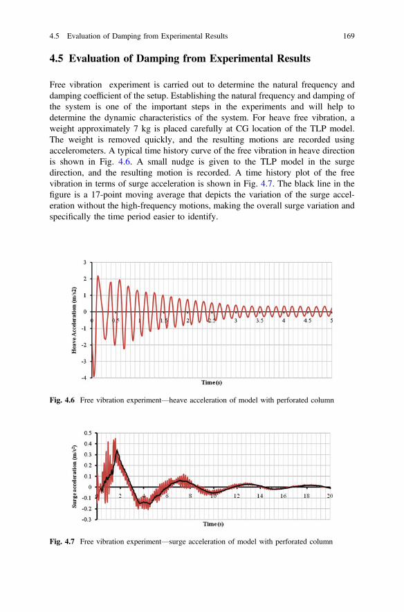
4.5 Evaluation of Damping from Experimental Results
Free vibration experiment is carried out to determine the natural frequency anddamping coefficient of the setup. Establishing the natural frequency and damping ofthe system is one of the important steps in the experiments and will help todetermine the dynamic characteristics of the system. For heave free vibration, aweight approximately 7 kg is placed carefully at CG location of the TLP model.The weight is removed quickly, and the resulting motions are recorded usingaccelerometers. A typical time history curve of the free vibration in heave directionis shown in Fig. 4.6. A small nudge is given to the TLP model in the surgedirection, and the resulting motion is recorded. A time history plot of the freevibration in terms of surge acceleration is shown in Fig. 4.7. The black line in thefigure is a 17-point moving average that depicts the variation of the surge accel-eration without the high-frequency motions, making the overall surge variation andspecifically the time period easier to identify.
Fig. 4.6 Free vibration experiment—heave acceleration of model with perforated column
Fig. 4.7 Free vibration experiment—surge acceleration of model with perforated column
4.5 Evaluation of Damping from Experimental Results 169
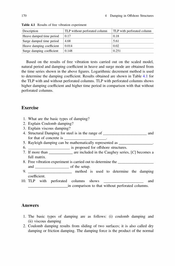
Based on the results of free vibration tests carried out on the scaled model,natural period and damping coefficient in heave and surge mode are obtained fromthe time series shown in the above figures. Logarithmic decrement method is usedto determine the damping coefficient. Results obtained are shown in Table 4.1 forthe TLP with and without perforated columns. TLP with perforated columns showshigher damping coefficient and higher time period in comparison with that withoutperforated columns.
Exercise
1. What are the basic types of damping?2. Explain Coulomb damping?3. Explain viscous damping?4. Structural Damping for steel is in the range of ______________________ and
for that of concrete is _____________________.5. Rayleigh damping can be mathematically represented as _________________.6. _____________________ is proposed for offshore structures.7. If more than ____________ are included in the Caughey series, [C] becomes a
full matrix.8. Free vibration experiment is carried out to determine the __________________
and _________________ of the setup.9. ______________________ method is used to determine the damping
coefficient.10. TLP with perforated columns shows ____________________ and
____________________in comparison to that without perforated columns.
Answers
1. The basic types of damping are as follows: (i) coulomb damping and(ii) viscous damping
2. Coulomb damping results from sliding of two surfaces; it is also called drydamping or friction damping. The damping force is the product of the normal
Table 4.1 Results of free vibration experiment
Description TLP without perforated column TLP with perforated column
Heave damped time period 0.17 0.18
Surge damped time period 4.68 5.61
Heave damping coefficient 0.014 0.02
Surge damping coefficient 0.148 0.251
170 4 Damping in Offshore Structures

force and the coefficient of friction between the body surface and the plane ofmotion. Note that the damping force in this case is independent of velocity ofmotion of the body which is under vibration.
3. Viscous damping, the damping force accounts for the viscosity of the system.The presence of fluid medium around the body significantly influences thedamping force acting on the body. Damping force will be proportional to themagnitude of the velocity and has the unit of N/(m s). Viscous damping seemsto be more relevant to offshore structural systems due to the inherent presenceof liquid medium around the body.
4. 0.2–0.5 % and 0.5–1.5 %.5. C = a0 M + a1K6. Rayleigh damping7. Two terms.8. Natural frequency and damping coefficient9. Logarithmic decrement
10. Higher damping coefficient and higher time period
Answers 171
Chapter 5Hydrodynamic Response of PerforatedOffshore Members
Abstract This chapter deals with hydrodynamic response of perforated cylindersunder regular waves through computational fluid dynamics (CFD). The chapterdeals with a brief introduction of fluid–structure interaction (FSI) and wave–structure interaction. Variations in water particle kinematics along the depth whenencountered by perforated members are discussed in detail as they find a lot ofrecent applications in the retrofitting and rehabilitation of offshore structuralmembers.
Keywords Hydrodynamic response � Experimental studies � Perforatedcylinders � Wave–structure interaction � Water particle kinematics � Retrofitting �Rehabilitation � Offshore structures � Tension leg platforms
5.1 Fluid–Structure Interaction
Fluid–structure interaction (FSI) plays an important role for structures placed in thepath of flowing fluid. The presence of structure alters fluid flow field in its vicinity.Degree of compliance offered by the structure adds further complexity due to thereaction it offers to the excited force. Even though structures remain flexible (e.g.,TLP) in certain degrees of freedom, dynamics becomes important. It is not theirdeformation capacity that is looked upon in this context. FSI becomes moreimportant when the flow is steady flow, may be in the form of current or a verticalshear. But in real sea state, structures experience large oscillating forces in the flowdirection. When structures are placed in the flowing fluid, the flow pattern is altered.Restraints are developed in the fluid medium to maintain the position of thestructure. Forces acting on the structures in fluid medium shall be classified as drag(acting in-line with the direction of flow) and lift (transverse to the direction offlow). Further, drag force can be classified as higher and smaller frequency com-ponents. These components will be functions of the geometry of the structure andflow conditions. Lift forces contain oscillatory components with multiple
© Springer India 2015S. Chandrasekaran, Dynamic Analysis and Design of Offshore Structures,Ocean Engineering & Oceanography 5, DOI 10.1007/978-81-322-2277-4_5
173
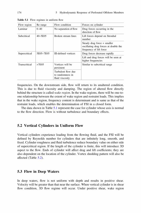
frequencies. On the downstream side, flow will return to its unaltered condition.This is due to fluid viscosity and damping. The region of altered flow directlybehind the structure is called wake region. In the wake regions, there will be one-to-one relationship between the extent of wake region and restraint loads. This impliesthat in the wake region, frequency content is determinant and is same as that of therestraint loads, which enables the determination of FSI in a closed form.
The data shown in Table 5.1 represent the case for cylinder whose axis is normalto the flow direction. Flow is without turbulence and boundary effects.
5.2 Vertical Cylinders in Uniform Flow
Vertical cylinders experience loading from the flowing fluid, and the FSI will bedefined by Reynolds number for cylinders that are infinitely long, smooth, andfixed. Cylinder roughness and fluid turbulence reduce boundary value on either sideof supercritical region. If the length of the cylinder is finite, this will introduce 3Daspect to the flow. Ends of cylinder will affect drag and lift coefficients; they arealso dependent on the location of the cylinder. Vortex shedding pattern will also beaffected (Table 5.2).
5.3 Flow in Deep Waters
In deep waters, flow is not uniform with depth and results in positive shear.Velocity will be greater than that near the surface. When vertical cylinder is in shearflow condition, 3D flow regime will occur. Under positive shear, wake region
Table 5.1 Flow regimes in uniform flow
Flow region Re range Flow condition Forces on cylinder
Laminar 0–40 No separation of flow Drag forces occurring in thedirection of flow
Subcritical 40–5E05 Broken stream lines Lift forces depend on Strouhalnumber
Steady drag force + smalleroscillating drag forces at double thefrequency of lift force
Supercritical 5E05–7E05 III-defined vortices Drag forces decrease rapidly
Lift and drag forces will be seen athigher frequencies
Transcritical >7E05 Vortices will bepersistent
Similar to subcritical range
Turbulent flow dueto randomness influid viscosity
174 5 Hydrodynamic Response of Perforated Offshore Members
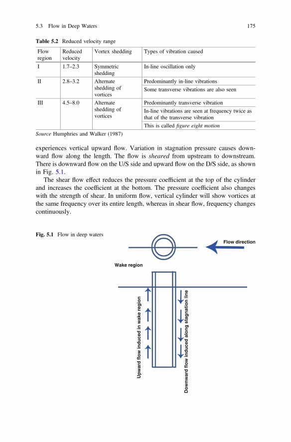
experiences vertical upward flow. Variation in stagnation pressure causes down-ward flow along the length. The flow is sheared from upstream to downstream.There is downward flow on the U/S side and upward flow on the D/S side, as shownin Fig. 5.1.
The shear flow effect reduces the pressure coefficient at the top of the cylinderand increases the coefficient at the bottom. The pressure coefficient also changeswith the strength of shear. In uniform flow, vertical cylinder will show vortices atthe same frequency over its entire length, whereas in shear flow, frequency changescontinuously.
Table 5.2 Reduced velocity range
Flowregion
Reducedvelocity
Vortex shedding Types of vibration caused
I 1.7–2.3 Symmetricshedding
In-line oscillation only
II 2.8–3.2 Alternateshedding ofvortices
Predominantly in-line vibrations
Some transverse vibrations are also seen
III 4.5–8.0 Alternateshedding ofvortices
Predominantly transverse vibration
In-line vibrations are seen at frequency twice asthat of the transverse vibration
This is called figure eight motion
Source Humphries and Walker (1987)
Wake region
Flow direction
Up
war
d f
low
ind
uce
d in
wak
e re
gio
n
Do
wn
war
d f
low
ind
uce
d a
lon
g s
tag
nat
ion
lin
e
Fig. 5.1 Flow in deep waters
5.3 Flow in Deep Waters 175
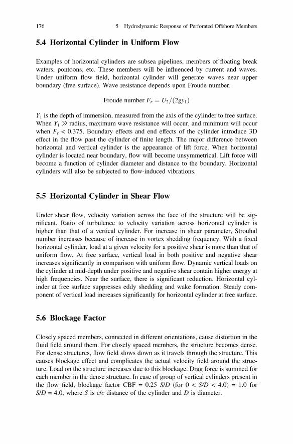
5.4 Horizontal Cylinder in Uniform Flow
Examples of horizontal cylinders are subsea pipelines, members of floating breakwaters, pontoons, etc. These members will be influenced by current and waves.Under uniform flow field, horizontal cylinder will generate waves near upperboundary (free surface). Wave resistance depends upon Froude number.
Froude number Fr ¼ U2= 2gy1ð Þ
Y1 is the depth of immersion, measured from the axis of the cylinder to free surface.When Y1 ≫ radius, maximum wave resistance will occur, and minimum will occurwhen Fr < 0.375. Boundary effects and end effects of the cylinder introduce 3Deffect in the flow past the cylinder of finite length. The major difference betweenhorizontal and vertical cylinder is the appearance of lift force. When horizontalcylinder is located near boundary, flow will become unsymmetrical. Lift force willbecome a function of cylinder diameter and distance to the boundary. Horizontalcylinders will also be subjected to flow-induced vibrations.
5.5 Horizontal Cylinder in Shear Flow
Under shear flow, velocity variation across the face of the structure will be sig-nificant. Ratio of turbulence to velocity variation across horizontal cylinder ishigher than that of a vertical cylinder. For increase in shear parameter, Strouhalnumber increases because of increase in vortex shedding frequency. With a fixedhorizontal cylinder, load at a given velocity for a positive shear is more than that ofuniform flow. At free surface, vertical load in both positive and negative shearincreases significantly in comparison with uniform flow. Dynamic vertical loads onthe cylinder at mid-depth under positive and negative shear contain higher energy athigh frequencies. Near the surface, there is significant reduction. Horizontal cyl-inder at free surface suppresses eddy shedding and wake formation. Steady com-ponent of vertical load increases significantly for horizontal cylinder at free surface.
5.6 Blockage Factor
Closely spaced members, connected in different orientations, cause distortion in thefluid field around them. For closely spaced members, the structure becomes dense.For dense structures, flow field slows down as it travels through the structure. Thiscauses blockage effect and complicates the actual velocity field around the struc-ture. Load on the structure increases due to this blockage. Drag force is summed foreach member in the dense structure. In case of group of vertical cylinders present inthe flow field, blockage factor CBF = 0.25 S/D (for 0 < S/D < 4.0) = 1.0 forS/D = 4.0, where S is c/c distance of the cylinder and D is diameter.
176 5 Hydrodynamic Response of Perforated Offshore Members
5.7 Wave–Structure Interaction (WSI)
When waves past cylinder, it causes oscillating in-line force on the cylinder. Inaddition, free surface also changes in case of a submerged cylinder. Large structuresplaced in wave field alter incident waves in its vicinity. If the dimension of thestructure is large compared to the wave length, flow remains attached to thestructure. When waves pass a cylinder, it causes oscillating in-line force on thecylinder. In addition, free surface also changes in case of a submerged cylinder.Several procedures can be used to explain the potential function generated in thevicinity, knowing the incident wave potential. Flow around the structure is assumedto remain attached. Separation is neglected and the fluid is assumed to be incom-pressible and irrotational, and structure is assumed to be rigid. Wave amplitude isassumed to be small. Fluid flow in the neighborhood is described by velocitypotential. Velocity potential under linear theory is given by:
U ¼ u eð�ixtÞ ð5:1Þ
where φ is spatial part of total velocity potential and ω is incident wave frequency.Total potential is the sum of potential of incident wave component and potential ofscattered wave component. Scattered wave component is normally represented bycontinuous distribution of waves. It is assumed as superposition of numerouswaves. Boundary value problem, defined in terms of Laplace partial differentialequations, is transformed into original partial differential equations, in potentialtheory. Boundary condition includes ocean floor, free surface, submerged surface ofthe structure, and radiation condition, as flow approaches infinity.
5.8 Perforated Cylinders
5.8.1 Wave Forces on Perforated Members
Several analytical studies are reported in the literature highlighting the wave forceson porous bodies. Wang and Ren (1994) are one of the earliest to study waveinteraction with a concentric surface-piercing porous outer cylinder protecting animpermeable inner cylinder. Free-surface elevation, net hydrodynamic forces, andwave-induced overturning moments on both cylinders are examined. Based on theanalytical investigations carried out, it is seen that inner cylinder experienced moreforces from long-period waves in comparison with that from short-period waves withdecrease in annular spacing between the outer perforated cylinder and inner cylinder.Results showed that the existence of exterior porous cylinder reduces hydrodynamicforce on the inner cylinder. Cylindrical breakwater is porous in the vicinity of the freesurface and impermeable at some distance below the free surface; significantreduction is reported in wave field and hydrodynamic forces experienced by the innercylinder (William and Li 1998). Interaction of waves with arrays of bottom-mounted,
5.7 Wave–Structure Interaction (WSI) 177
surface-piercing circular cylinders is investigated through numerical studies(Williams and Li 2000). It is shown that the porosity of the structure results in asignificant reduction in both the hydrodynamic loads experienced by the cylindersand the associated wave run-up. William et al. (2000) investigated the interaction ofwaves and free-floating circular cylinder with porous side walls. The porous region isbounded on top and bottom by impermeable end caps, which resulted in an enclosedfluid region within the structure. It is found that the permeability, size, and location ofthe porous region have a significant influence on the horizontal component of thehydrodynamic excitation and reaction loads, while their influence on the verticalcomponents is relatively minor. Neelamani et al. (2002) carried out experimentalinvestigations of seawater intake structure consisting of a perforated square caissonencircling a vertical suction through physical model studies. They found that the ratioof force on perforated caisson to the force on caisson with 10% porosity is reduced toa maximum of 60 % with increase in the porosity of the caisson from 1.6 to 16.9 %.This ratio is found to increase with the increase in relative wave height and decreasewith increase in relative width. Neelamani and Muni (2002) examined wave forceson a vertical cylinder protected by vertical and inclined perforated barriers;numerical studies showed that there is a significant reduction in forces on the verticalcylinder due to perforated barriers.
Song and Tao (2007) studied 3D short-crested wave interaction with a con-centric porous cylindrical structure. It is recommended that porous effect should bechosen lesser than 2 in order to provide meaningful protection to the interiorcylinder from the wave impact. Vijayalakshmi et al. (2008) carried out experimentalinvestigations on perforated circular cylinder encircling an impermeable cylinder ata constant water depth for regular and random waves. Porosity of the outer cylinderis varied from 4.54 to 19.15 % to study its influence on variations in wave forces inthe vicinity of the chosen twin-cylinder system. Numerical method is developed onthe basis of the application of boundary integral equation on a porous body withappropriate boundary conditions; porosity is modeled using the resistance coeffi-cient and added mass coefficient for regular waves. It is seen that the resistancecoefficient increased with the increase in porosity and wave height except for aporosity of 4.54 %; added mass coefficient is almost negligible. Based on theexperimental results, porosity of 10–15 % is recommended to have significant effecton force reduction. Sankarbabu et al. (2007) investigated the influence of hydro-dynamic wave forces on a group of cylinders, wave run-up, and free-surface ele-vation in their vicinity. Results showed that the forces on inner cylinders arereduced in the presence of an outer porous cylinder when compared to that of thedirect wave impact. Sankarbabu et al. (2007) investigated the hydrodynamic per-formance of a dual cylindrical caisson breakwater (DCBW) that is formed by a rowof caissons; these caissons consist of porous outer cylinder circumscribing animpermeable inner cylinder. Based on the analytical studies carried out, it is seenthat an optimum ratio of radius of inner cylinder to the outer exists as 0.5 for asatisfactory hydrodynamic performance of the DCBW; it shows improved stabilityand wave transformation in its vicinity. Further, they concluded that the influence ofporosity on the variation of forces, run-up on the caissons, and the surface elevation
178 5 Hydrodynamic Response of Perforated Offshore Members
in the vicinity of the DCBW are found to be significant up to a value of 1.0; anyfurther increase in this value results in lesser variation of the above parameters.Zhao et al. (2009) studied the interaction of waves and a porous cylinder with aninner horizontal porous plate; effects of porosity and position of the inner plate areinvestigated. It is shown that increase in porosity reduces wave exciting forces andefficiency of wave dissipation; inner plate eliminates the sloshing mode in surge andpitch degrees of freedom. The arrangement is recommended for effective waveenergy dissipation when located at still water surface.
5.8.2 Wave Forces on Offshore Structures with PerforatedMembers
Ker and Lee (2002) examined the coupling problems associated with wave–structureinteraction (WSI) of linear waves and porous tension leg platform (TLP),analytically. They found that the drag force in the porous body changes the responsebehavior of TLP significantly; at resonance frequencies, this change is significant.They also found that for long-period waves, porous TLP remains relatively trans-parent and is similar to that of an impermeable one, while it dissipates most of thewave energy for short-period waves. Zhong and Wang (2006) carried out analyticalstudies on solitary waves interacting with surface-piercing concentric porous cyl-inders. It was found that the hydrodynamic forces on inner cylinder increase and thatof the exterior cylinder decrease with the decrease in the annular spacing. Forces on asingle porous cylinder are reduced significantly in comparison with that of animpermeable cylinder of the same diameter. Further, it is also shown that for largerporosity of the outer cylinder, larger hydrodynamic forces are encountered on theinner cylinder and lesser on the outer cylinder. Existence of exterior porous cylinderreduces hydrodynamic force on the interior cylinder. Vijayalakshmi et al. (2007)verified this fact through experimental investigations by measuring wave forces andrun-up on the twin, concentric perforated cylinders; results are compared with thosepredicted by the boundary integral method and found satisfactory. Porous effects onthin permeable plates are well quantified by Li et al. (2006); predicted values ofporous effects of reflection and transmission coefficients that are estimated usinganalytical model are validated with experimental results. Jayalekshmi et al. (2010)investigated the dynamic response of a TLP under random waves and the effect ofriser dynamics on platform behavior; an in-house finite element code is developed bythe authors to perform the analysis. A random sea state is generated using the PMspectrum. Water particle kinematics is calculated using Airy’s linear wave theory,and the load is evaluated using the relative form of the Morrison equation; variablesubmergence and current forces are also taken into account.
Adrezin et al. (1996) carried out dynamic analysis of complaint offshore struc-tures and reiterated the fact that coupled motion analysis induces significantresponse in all active degrees of freedom of TLP under linear waves. Kim et al.(2007) discussed various nonlinearities associated with the analysis of TLPs under
5.8 Perforated Cylinders 179
regular waves; the effect of these nonlinearities on the dynamic response andvarious strategies to solve the equation of motion for the fully coupled dynamicanalysis are discussed in detail (Chakrabarti 1984, 1987, 1994). Zeng et al. (2007)conducted parametric studies of TLPs with large amplitude motion. Dynamicresponse predicted by linear and nonlinear models are compared; they showed thatthe nonlinear responses of TLP, considering the effects induced by large amplitudemotions, differ from that of the linear model, significantly. Two different approa-ches for response calculations are compared with wave approach angle as one of theprimary factors in the parametric study. Kurian et al. (2008) conducted parametricstudies on TLPs under random waves. Authors used PM spectrum, Airy wavetheory, relative form of Morrison equation, and Newmark-Beta time integrationscheme to obtain the response in time domain. Mass, damping and stiffnessmatrices that are required to calculate the response are derived from the literature(Chandrasekaran and Jain 2002; Chandrasekaran et al. 2004). Although coefficientsused in the process of determining response are on the basis of recommendationsmade by other authors, both numerical and experimental investigations carried outby the authors are considered valid due to a close comparison of the same. Studiesare also carried out by researchers to illustrate the influence of wave approach angleon the response of TLP in regular sea (Chandrasekaran et al. 2007; Kim et al. 2007).Numerical studies carried out on triangular TLP under a variety of wave approachangles showed that nonlinear Stokes’s fifth-order wave theory is well suited fordeep-sea structures such as TLPs to estimate dynamic response. Significance ofother nonlinearities caused by change in tether tension and variable submergenceeffect is on the dynamic response of TLPs are also highlighted in the studies.Experimental studies carried out on the response analysis of TLPs showed the scaleeffect on the response quantities; variations between the analytical and experimentalresults are attributed to the boundary effect on the scaled model during experiments(Joseph et al. 2004).
5.8.3 Critical Review
A detailed review of the literature on wave interaction on porous cylinders ispresented. Influence of porous region on the forces experienced by inner cylinder inthe presence of perforated outer cover is highlighted. Both experimental and ana-lytical studies carried out by various researchers show a common agreement ofsignificant force reduction on the inner cylinder with perforated outer cover. Severalstudies highlighting the dynamic response of offshore TLPs under regular andrandom waves are also discussed; various nonlinearities associated with theresponse behavior of TLPs under waves are presented. Few experimental investi-gations carried out on dynamic response of TLP with perforated members are alsodiscussed. It is seen from the above review that experimental investigations ondynamic response of TLPs with perforated outer cover are scarce in the literature;hence, the current research study justifies the defined objectives.
180 5 Hydrodynamic Response of Perforated Offshore Members
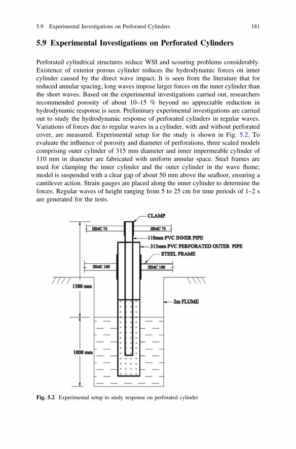
5.9 Experimental Investigations on Perforated Cylinders
Perforated cylindrical structures reduce WSI and scouring problems considerably.Existence of exterior porous cylinder reduces the hydrodynamic forces on innercylinder caused by the direct wave impact. It is seen from the literature that forreduced annular spacing, long waves impose larger forces on the inner cylinder thanthe short waves. Based on the experimental investigations carried out, researchersrecommended porosity of about 10–15 % beyond no appreciable reduction inhydrodynamic response is seen. Preliminary experimental investigations are carriedout to study the hydrodynamic response of perforated cylinders in regular waves.Variations of forces due to regular waves in a cylinder, with and without perforatedcover, are measured. Experimental setup for the study is shown in Fig. 5.2. Toevaluate the influence of porosity and diameter of perforations, three scaled modelscomprising outer cylinder of 315 mm diameter and inner impermeable cylinder of110 mm in diameter are fabricated with uniform annular space. Steel frames areused for clamping the inner cylinder and the outer cylinder in the wave flume;model is suspended with a clear gap of about 50 mm above the seafloor, ensuring acantilever action. Strain gauges are placed along the inner cylinder to determine theforces. Regular waves of height ranging from 5 to 25 cm for time periods of 1–2 sare generated for the tests.
Fig. 5.2 Experimental setup to study response on perforated cylinder
5.9 Experimental Investigations on Perforated Cylinders 181
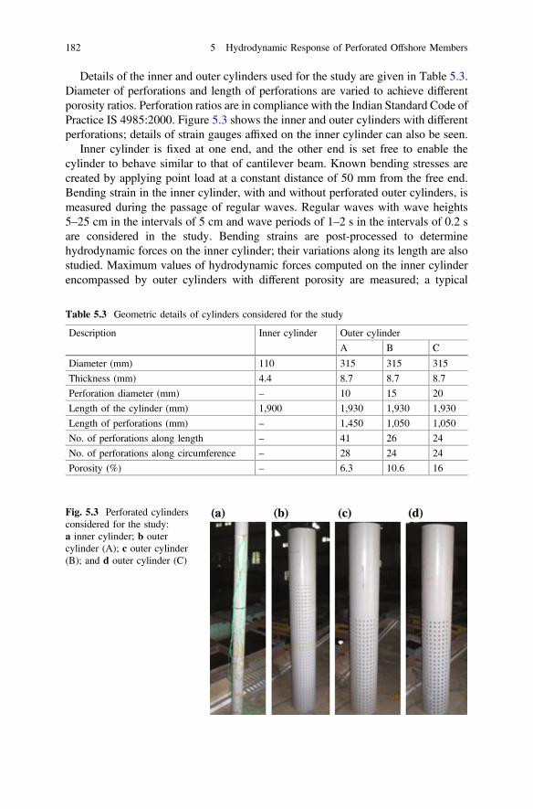
Details of the inner and outer cylinders used for the study are given in Table 5.3.Diameter of perforations and length of perforations are varied to achieve differentporosity ratios. Perforation ratios are in compliance with the Indian Standard Code ofPractice IS 4985:2000. Figure 5.3 shows the inner and outer cylinders with differentperforations; details of strain gauges affixed on the inner cylinder can also be seen.
Inner cylinder is fixed at one end, and the other end is set free to enable thecylinder to behave similar to that of cantilever beam. Known bending stresses arecreated by applying point load at a constant distance of 50 mm from the free end.Bending strain in the inner cylinder, with and without perforated outer cylinders, ismeasured during the passage of regular waves. Regular waves with wave heights5–25 cm in the intervals of 5 cm and wave periods of 1–2 s in the intervals of 0.2 sare considered in the study. Bending strains are post-processed to determinehydrodynamic forces on the inner cylinder; their variations along its length are alsostudied. Maximum values of hydrodynamic forces computed on the inner cylinderencompassed by outer cylinders with different porosity are measured; a typical
Table 5.3 Geometric details of cylinders considered for the study
Description Inner cylinder Outer cylinder
A B C
Diameter (mm) 110 315 315 315
Thickness (mm) 4.4 8.7 8.7 8.7
Perforation diameter (mm) – 10 15 20
Length of the cylinder (mm) 1,900 1,930 1,930 1,930
Length of perforations (mm) – 1,450 1,050 1,050
No. of perforations along length – 41 26 24
No. of perforations along circumference – 28 24 24
Porosity (%) – 6.3 10.6 16
Fig. 5.3 Perforated cylindersconsidered for the study:a inner cylinder; b outercylinder (A); c outer cylinder(B); and d outer cylinder (C)
182 5 Hydrodynamic Response of Perforated Offshore Members
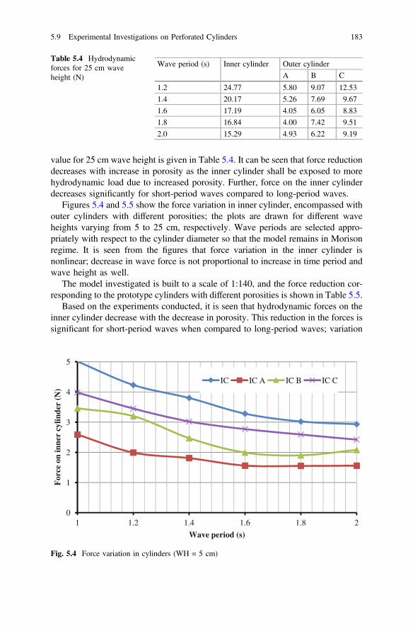
value for 25 cm wave height is given in Table 5.4. It can be seen that force reductiondecreases with increase in porosity as the inner cylinder shall be exposed to morehydrodynamic load due to increased porosity. Further, force on the inner cylinderdecreases significantly for short-period waves compared to long-period waves.
Figures 5.4 and 5.5 show the force variation in inner cylinder, encompassed withouter cylinders with different porosities; the plots are drawn for different waveheights varying from 5 to 25 cm, respectively. Wave periods are selected appro-priately with respect to the cylinder diameter so that the model remains in Morisonregime. It is seen from the figures that force variation in the inner cylinder isnonlinear; decrease in wave force is not proportional to increase in time period andwave height as well.
The model investigated is built to a scale of 1:140, and the force reduction cor-responding to the prototype cylinders with different porosities is shown in Table 5.5.
Based on the experiments conducted, it is seen that hydrodynamic forces on theinner cylinder decrease with the decrease in porosity. This reduction in the forces issignificant for short-period waves when compared to long-period waves; variation
Table 5.4 Hydrodynamicforces for 25 cm waveheight (N)
Wave period (s) Inner cylinder Outer cylinder
A B C
1.2 24.77 5.80 9.07 12.53
1.4 20.17 5.26 7.69 9.67
1.6 17.19 4.05 6.05 8.83
1.8 16.84 4.00 7.42 9.51
2.0 15.29 4.93 6.22 9.19
0
1
2
3
4
5
1 1.2 1.4 1.6 1.8 2
For
ce o
n in
ner
cylin
der
(N)
Wave period (s)
IC IC A IC B IC C
Fig. 5.4 Force variation in cylinders (WH = 5 cm)
5.9 Experimental Investigations on Perforated Cylinders 183
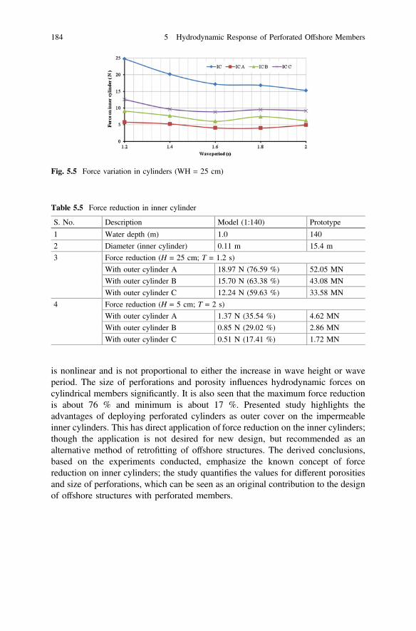
is nonlinear and is not proportional to either the increase in wave height or waveperiod. The size of perforations and porosity influences hydrodynamic forces oncylindrical members significantly. It is also seen that the maximum force reductionis about 76 % and minimum is about 17 %. Presented study highlights theadvantages of deploying perforated cylinders as outer cover on the impermeableinner cylinders. This has direct application of force reduction on the inner cylinders;though the application is not desired for new design, but recommended as analternative method of retrofitting of offshore structures. The derived conclusions,based on the experiments conducted, emphasize the known concept of forcereduction on inner cylinders; the study quantifies the values for different porositiesand size of perforations, which can be seen as an original contribution to the designof offshore structures with perforated members.
Table 5.5 Force reduction in inner cylinder
S. No. Description Model (1:140) Prototype
1 Water depth (m) 1.0 140
2 Diameter (inner cylinder) 0.11 m 15.4 m
3 Force reduction (H = 25 cm; T = 1.2 s)
With outer cylinder A 18.97 N (76.59 %) 52.05 MN
With outer cylinder B 15.70 N (63.38 %) 43.08 MN
With outer cylinder C 12.24 N (59.63 %) 33.58 MN
4 Force reduction (H = 5 cm; T = 2 s)
With outer cylinder A 1.37 N (35.54 %) 4.62 MN
With outer cylinder B 0.85 N (29.02 %) 2.86 MN
With outer cylinder C 0.51 N (17.41 %) 1.72 MN
Fig. 5.5 Force variation in cylinders (WH = 25 cm)
184 5 Hydrodynamic Response of Perforated Offshore Members
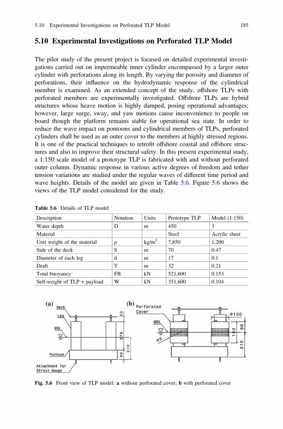
5.10 Experimental Investigations on Perforated TLP Model
The pilot study of the present project is focused on detailed experimental investi-gations carried out on impermeable inner cylinder encompassed by a larger outercylinder with perforations along its length. By varying the porosity and diameter ofperforations, their influence on the hydrodynamic response of the cylindricalmember is examined. As an extended concept of the study, offshore TLPs withperforated members are experimentally investigated. Offshore TLPs are hybridstructures whose heave motion is highly damped, posing operational advantages;however, large surge, sway, and yaw motions cause inconvenience to people onboard though the platform remains stable for operational sea state. In order toreduce the wave impact on pontoons and cylindrical members of TLPs, perforatedcylinders shall be used as an outer cover to the members at highly stressed regions.It is one of the practical techniques to retrofit offshore coastal and offshore struc-tures and also to improve their structural safety. In this present experimental study,a 1:150 scale model of a prototype TLP is fabricated with and without perforatedouter column. Dynamic response in various active degrees of freedom and tethertension variations are studied under the regular waves of different time period andwave heights. Details of the model are given in Table 5.6. Figure 5.6 shows theviews of the TLP model considered for the study.
Table 5.6 Details of TLP model
Description Notation Units Prototype TLP Model (1:150)
Water depth D m 450 3
Material Steel Acrylic sheet
Unit weight of the material ρ kg/m3 7,850 1,200
Side of the deck S m 70 0.47
Diameter of each leg d m 17 0.1
Draft T m 32 0.21
Total buoyancy FB kN 521,600 0.153
Self-weight of TLP + payload W kN 351,600 0.104
Fig. 5.6 Front view of TLP model: a without perforated cover; b with perforated cover
5.10 Experimental Investigations on Perforated TLP Model 185
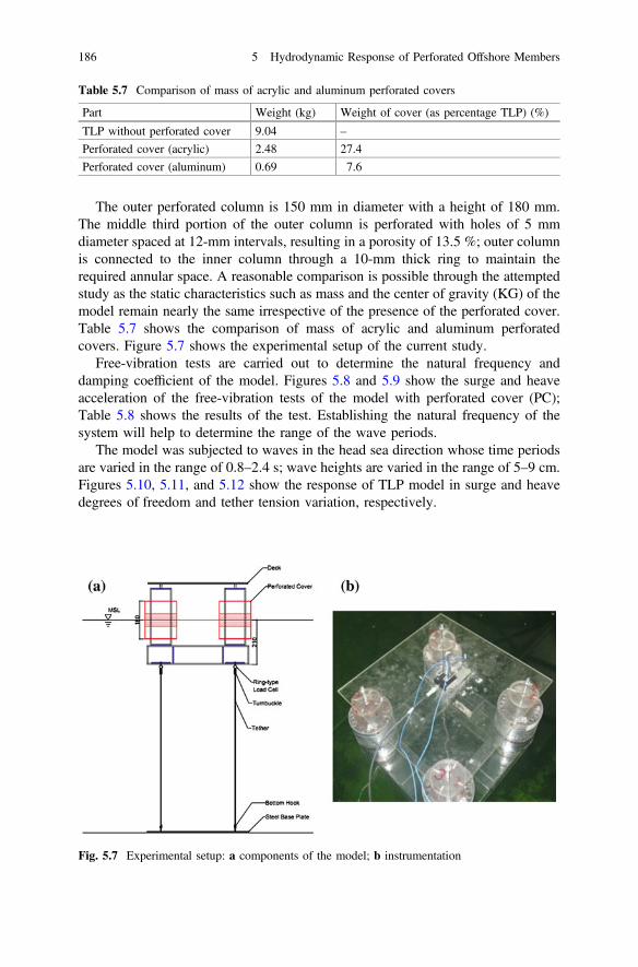
The outer perforated column is 150 mm in diameter with a height of 180 mm.The middle third portion of the outer column is perforated with holes of 5 mmdiameter spaced at 12-mm intervals, resulting in a porosity of 13.5 %; outer columnis connected to the inner column through a 10-mm thick ring to maintain therequired annular space. A reasonable comparison is possible through the attemptedstudy as the static characteristics such as mass and the center of gravity (KG) of themodel remain nearly the same irrespective of the presence of the perforated cover.Table 5.7 shows the comparison of mass of acrylic and aluminum perforatedcovers. Figure 5.7 shows the experimental setup of the current study.
Free-vibration tests are carried out to determine the natural frequency anddamping coefficient of the model. Figures 5.8 and 5.9 show the surge and heaveacceleration of the free-vibration tests of the model with perforated cover (PC);Table 5.8 shows the results of the test. Establishing the natural frequency of thesystem will help to determine the range of the wave periods.
The model was subjected to waves in the head sea direction whose time periodsare varied in the range of 0.8–2.4 s; wave heights are varied in the range of 5–9 cm.Figures 5.10, 5.11, and 5.12 show the response of TLP model in surge and heavedegrees of freedom and tether tension variation, respectively.
Table 5.7 Comparison of mass of acrylic and aluminum perforated covers
Part Weight (kg) Weight of cover (as percentage TLP) (%)
TLP without perforated cover 9.04 –
Perforated cover (acrylic) 2.48 27.4
Perforated cover (aluminum) 0.69 7.6
Fig. 5.7 Experimental setup: a components of the model; b instrumentation
186 5 Hydrodynamic Response of Perforated Offshore Members
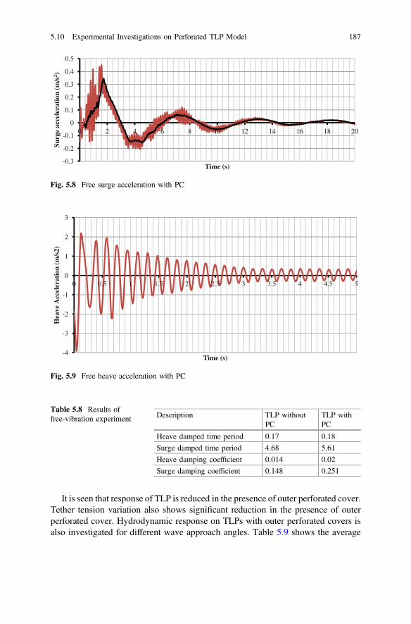
It is seen that response of TLP is reduced in the presence of outer perforated cover.Tether tension variation also shows significant reduction in the presence of outerperforated cover. Hydrodynamic response on TLPs with outer perforated covers isalso investigated for different wave approach angles. Table 5.9 shows the average
-0.3
-0.2
-0.1
0
0.1
0.2
0.3
0.4
0.5
0 2 4 6 8 10 12 14 16 18 20
Surg
e ac
cele
rati
on (m
/s2 )
Time (s)
Fig. 5.8 Free surge acceleration with PC
-4
-3
-2
-1
0
1
2
3
0 0.5 1 1.5 2 2.5 3 3.5 4 4.5 5
Hea
ve A
ccel
erat
ion
(m/s
2)
Time (s)
Fig. 5.9 Free heave acceleration with PC
Table 5.8 Results offree-vibration experiment Description TLP without
PCTLP withPC
Heave damped time period 0.17 0.18
Surge damped time period 4.68 5.61
Heave damping coefficient 0.014 0.02
Surge damping coefficient 0.148 0.251
5.10 Experimental Investigations on Perforated TLP Model 187
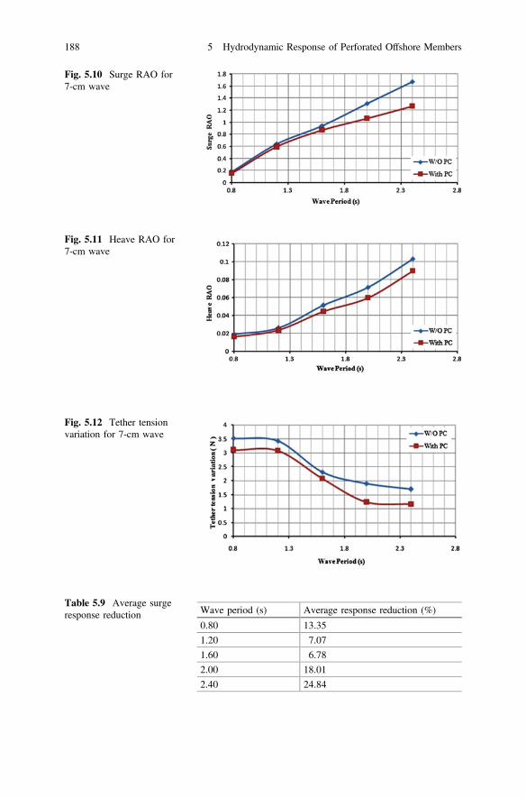
Fig. 5.10 Surge RAO for7-cm wave
Fig. 5.11 Heave RAO for7-cm wave
Fig. 5.12 Tether tensionvariation for 7-cm wave
Table 5.9 Average surgeresponse reduction Wave period (s) Average response reduction (%)
0.80 13.35
1.20 7.07
1.60 6.78
2.00 18.01
2.40 24.84
188 5 Hydrodynamic Response of Perforated Offshore Members

reduction in surge response for different wave periods; the maximum responsereduction seen is about 24 % due to the presence of outer perforated cylinders.
Presented study highlights the advantages of deploying perforated columnmembers for TLP as outer cover on the impermeable inner cylinders. This has directapplication of force reduction on the inner cylinders; though the application is notdesired for new design, but recommended as an alternative method of retrofitting ofoffshore structures.
5.11 Numerical Studies on Perforated Cylinders
Numerical studies on perforated cylinders are carried out through simulation inSTAR-CCM+ software. An attempt is made to simulate the hydrodynamic responseof perforated cylinder with porosity 6.3 %, which is similar to that of perforatedouter cylinder, designated as A in the experimental studies. Simulation throughSTAR-CCM+ software is chosen due to the numerical capabilities enabled indifferent modules to simulate viscous drag and turbulence effects that are caused byperforations. Details of the simulation, as attempted through several stages of thenumerical modeling, are discussed in steps; various settings such as mesh andphysics models used in the study and their significance are also presented.
5.11.1 Development of the Numerical Models
A model of the perforated cylinder is CATIA V5. Figure 5.13 shows the model ofthe perforated outer cylinder generated in the software. Table 5.10 shows the detailsof both inner and perforated outer cylinder, while Table 5.11 shows the details ofthe perforations. Using ‘Pocket’ tool, perforations are created along the circum-ference and length of the outer cylinder using ‘Circular pattern’ and ‘Rectangularpattern’ tools, respectively. Figures 5.14 and 5.15 show images of outer perforatedcylinder and the assembly of inner with perforated outer cylinder, respectively.
Fig. 5.13 Perforated outercylinder
5.10 Experimental Investigations on Perforated TLP Model 189
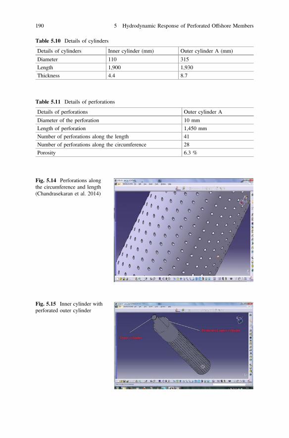
Table 5.10 Details of cylinders
Details of cylinders Inner cylinder (mm) Outer cylinder A (mm)
Diameter 110 315
Length 1,900 1,930
Thickness 4.4 8.7
Table 5.11 Details of perforations
Details of perforations Outer cylinder A
Diameter of the perforation 10 mm
Length of perforation 1,450 mm
Number of perforations along the length 41
Number of perforations along the circumference 28
Porosity 6.3 %
Fig. 5.15 Inner cylinder withperforated outer cylinder
Fig. 5.14 Perforations alongthe circumference and length(Chandrasekaran et al. 2014)
190 5 Hydrodynamic Response of Perforated Offshore Members
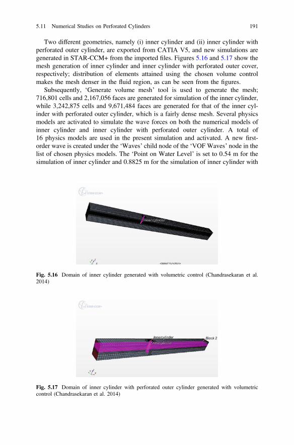
Two different geometries, namely (i) inner cylinder and (ii) inner cylinder withperforated outer cylinder, are exported from CATIA V5, and new simulations aregenerated in STAR-CCM+ from the imported files. Figures 5.16 and 5.17 show themesh generation of inner cylinder and inner cylinder with perforated outer cover,respectively; distribution of elements attained using the chosen volume controlmakes the mesh denser in the fluid region, as can be seen from the figures.
Subsequently, ‘Generate volume mesh’ tool is used to generate the mesh;716,801 cells and 2,167,056 faces are generated for simulation of the inner cylinder,while 3,242,875 cells and 9,671,484 faces are generated for that of the inner cyl-inder with perforated outer cylinder, which is a fairly dense mesh. Several physicsmodels are activated to simulate the wave forces on both the numerical models ofinner cylinder and inner cylinder with perforated outer cylinder. A total of16 physics models are used in the present simulation and activated. A new first-order wave is created under the ‘Waves’ child node of the ‘VOF Waves’ node in thelist of chosen physics models. The ‘Point on Water Level’ is set to 0.54 m for thesimulation of inner cylinder and 0.8825 m for the simulation of inner cylinder with
Fig. 5.16 Domain of inner cylinder generated with volumetric control (Chandrasekaran et al.2014)
Fig. 5.17 Domain of inner cylinder with perforated outer cylinder generated with volumetriccontrol (Chandrasekaran et al. 2014)
5.11 Numerical Studies on Perforated Cylinders 191
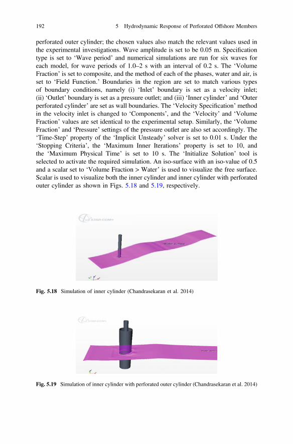
perforated outer cylinder; the chosen values also match the relevant values used inthe experimental investigations. Wave amplitude is set to be 0.05 m. Specificationtype is set to ‘Wave period’ and numerical simulations are run for six waves foreach model, for wave periods of 1.0–2 s with an interval of 0.2 s. The ‘VolumeFraction’ is set to composite, and the method of each of the phases, water and air, isset to ‘Field Function.’ Boundaries in the region are set to match various typesof boundary conditions, namely (i) ‘Inlet’ boundary is set as a velocity inlet;(ii) ‘Outlet’ boundary is set as a pressure outlet; and (iii) ‘Inner cylinder’ and ‘Outerperforated cylinder’ are set as wall boundaries. The ‘Velocity Specification’ methodin the velocity inlet is changed to ‘Components’, and the ‘Velocity’ and ‘VolumeFraction’ values are set identical to the experimental setup. Similarly, the ‘VolumeFraction’ and ‘Pressure’ settings of the pressure outlet are also set accordingly. The‘Time-Step’ property of the ‘Implicit Unsteady’ solver is set to 0.01 s. Under the‘Stopping Criteria’, the ‘Maximum Inner Iterations’ property is set to 10, andthe ‘Maximum Physical Time’ is set to 10 s. The ‘Initialize Solution’ tool isselected to activate the required simulation. An iso-surface with an iso-value of 0.5and a scalar set to ‘Volume Fraction > Water’ is used to visualize the free surface.Scalar is used to visualize both the inner cylinder and inner cylinder with perforatedouter cylinder as shown in Figs. 5.18 and 5.19, respectively.
Fig. 5.18 Simulation of inner cylinder (Chandrasekaran et al. 2014)
Fig. 5.19 Simulation of inner cylinder with perforated outer cylinder (Chandrasekaran et al. 2014)
192 5 Hydrodynamic Response of Perforated Offshore Members
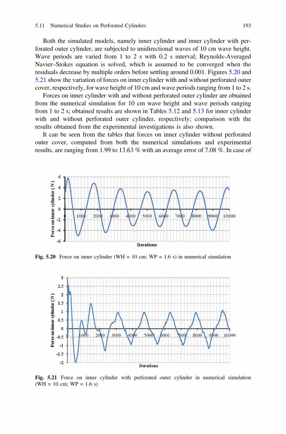
Both the simulated models, namely inner cylinder and inner cylinder with per-forated outer cylinder, are subjected to unidirectional waves of 10 cm wave height.Wave periods are varied from 1 to 2 s with 0.2 s interval; Reynolds-AveragedNavier–Stokes equation is solved, which is assumed to be converged when theresiduals decrease by multiple orders before settling around 0.001. Figures 5.20 and5.21 show the variation of forces on inner cylinder with and without perforated outercover, respectively, for wave height of 10 cm and wave periods ranging from 1 to 2 s.
Forces on inner cylinder with and without perforated outer cylinder are obtainedfrom the numerical simulation for 10 cm wave height and wave periods rangingfrom 1 to 2 s; obtained results are shown in Tables 5.12 and 5.13 for inner cylinderwith and without perforated outer cylinder, respectively; comparison with theresults obtained from the experimental investigations is also shown.
It can be seen from the tables that forces on inner cylinder without perforatedouter cover, computed from both the numerical simulations and experimentalresults, are ranging from 1.99 to 13.63 % with an average error of 7.08 %. In case of
Fig. 5.20 Force on inner cylinder (WH = 10 cm; WP = 1.6 s) in numerical simulation
Fig. 5.21 Force on inner cylinder with perforated outer cylinder in numerical simulation(WH = 10 cm; WP = 1.6 s)
5.11 Numerical Studies on Perforated Cylinders 193
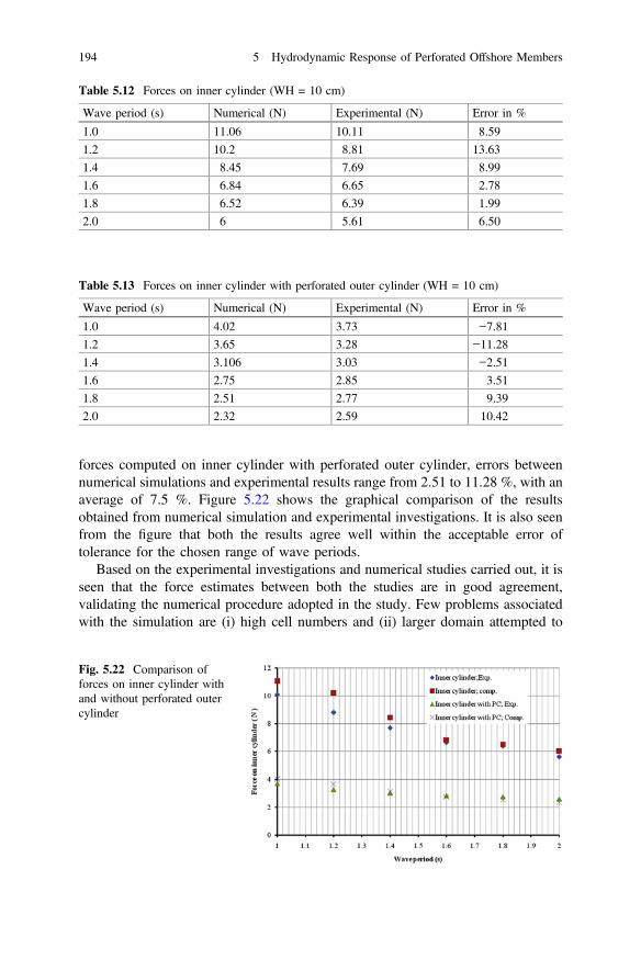
forces computed on inner cylinder with perforated outer cylinder, errors betweennumerical simulations and experimental results range from 2.51 to 11.28 %, with anaverage of 7.5 %. Figure 5.22 shows the graphical comparison of the resultsobtained from numerical simulation and experimental investigations. It is also seenfrom the figure that both the results agree well within the acceptable error oftolerance for the chosen range of wave periods.
Based on the experimental investigations and numerical studies carried out, it isseen that the force estimates between both the studies are in good agreement,validating the numerical procedure adopted in the study. Few problems associatedwith the simulation are (i) high cell numbers and (ii) larger domain attempted to
Table 5.12 Forces on inner cylinder (WH = 10 cm)
Wave period (s) Numerical (N) Experimental (N) Error in %
1.0 11.06 10.11 8.59
1.2 10.2 8.81 13.63
1.4 8.45 7.69 8.99
1.6 6.84 6.65 2.78
1.8 6.52 6.39 1.99
2.0 6 5.61 6.50
Table 5.13 Forces on inner cylinder with perforated outer cylinder (WH = 10 cm)
Wave period (s) Numerical (N) Experimental (N) Error in %
1.0 4.02 3.73 −7.81
1.2 3.65 3.28 −11.28
1.4 3.106 3.03 −2.51
1.6 2.75 2.85 3.51
1.8 2.51 2.77 9.39
2.0 2.32 2.59 10.42
Fig. 5.22 Comparison offorces on inner cylinder withand without perforated outercylinder
194 5 Hydrodynamic Response of Perforated Offshore Members
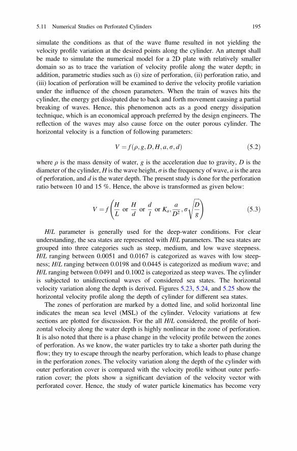
simulate the conditions as that of the wave flume resulted in not yielding thevelocity profile variation at the desired points along the cylinder. An attempt shallbe made to simulate the numerical model for a 2D plate with relatively smallerdomain so as to trace the variation of velocity profile along the water depth; inaddition, parametric studies such as (i) size of perforation, (ii) perforation ratio, and(iii) location of perforation will be examined to derive the velocity profile variationunder the influence of the chosen parameters. When the train of waves hits thecylinder, the energy get dissipated due to back and forth movement causing a partialbreaking of waves. Hence, this phenomenon acts as a good energy dissipationtechnique, which is an economical approach preferred by the design engineers. Thereflection of the waves may also cause force on the outer porous cylinder. Thehorizontal velocity is a function of following parameters:
V ¼ f ðq; g;D;H; a; r; dÞ ð5:2Þ
where ρ is the mass density of water, g is the acceleration due to gravity, D is thediameter of the cylinder,H is the wave height, σ is the frequency of wave, a is the areaof perforation, and d is the water depth. The present study is done for the perforationratio between 10 and 15 %. Hence, the above is transformed as given below:
V ¼ fHL
orHd
ordlor Ka;
aD2 ; r
ffiffiffiffiDg
s !ð5:3Þ
H/L parameter is generally used for the deep-water conditions. For clearunderstanding, the sea states are represented with H/L parameters. The sea states aregrouped into three categories such as steep, medium, and low wave steepness.H/L ranging between 0.0051 and 0.0167 is categorized as waves with low steep-ness; H/L ranging between 0.0198 and 0.0445 is categorized as medium wave; andH/L ranging between 0.0491 and 0.1002 is categorized as steep waves. The cylinderis subjected to unidirectional waves of considered sea states. The horizontalvelocity variation along the depth is derived. Figures 5.23, 5.24, and 5.25 show thehorizontal velocity profile along the depth of cylinder for different sea states.
The zones of perforation are marked by a dotted line, and solid horizontal lineindicates the mean sea level (MSL) of the cylinder. Velocity variations at fewsections are plotted for discussion. For the all H/L considered, the profile of hori-zontal velocity along the water depth is highly nonlinear in the zone of perforation.It is also noted that there is a phase change in the velocity profile between the zonesof perforation. As we know, the water particles try to take a shorter path during theflow; they try to escape through the nearby perforation, which leads to phase changein the perforation zones. The velocity variation along the depth of the cylinder withouter perforation cover is compared with the velocity profile without outer perfo-ration cover; the plots show a significant deviation of the velocity vector withperforated cover. Hence, the study of water particle kinematics has become very
5.11 Numerical Studies on Perforated Cylinders 195
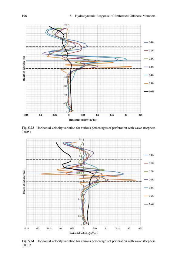
Fig. 5.24 Horizontal velocity variation for various percentages of perforation with wave steepness0.0103
Fig. 5.23 Horizontal velocity variation for various percentages of perforation with wave steepness0.0051
196 5 Hydrodynamic Response of Perforated Offshore Members
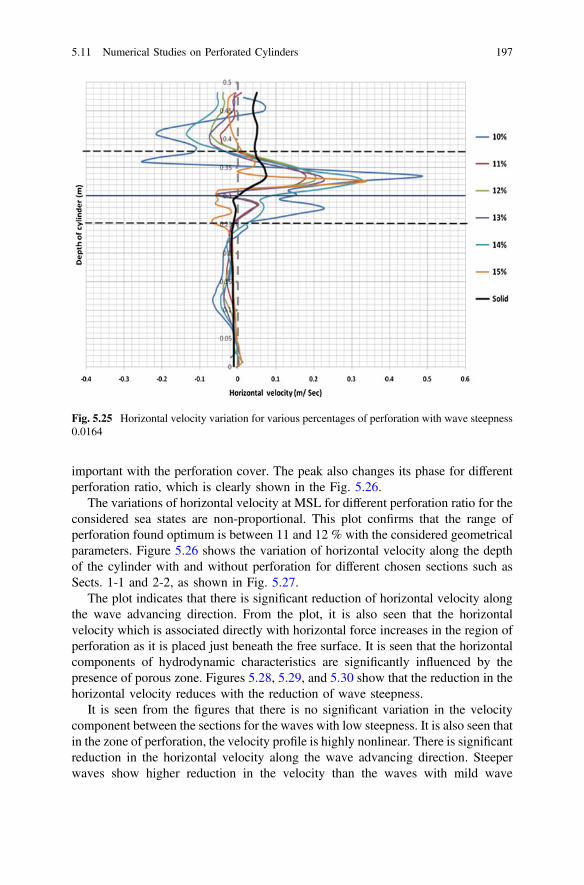
important with the perforation cover. The peak also changes its phase for differentperforation ratio, which is clearly shown in the Fig. 5.26.
The variations of horizontal velocity at MSL for different perforation ratio for theconsidered sea states are non-proportional. This plot confirms that the range ofperforation found optimum is between 11 and 12 % with the considered geometricalparameters. Figure 5.26 shows the variation of horizontal velocity along the depthof the cylinder with and without perforation for different chosen sections such asSects. 1-1 and 2-2, as shown in Fig. 5.27.
The plot indicates that there is significant reduction of horizontal velocity alongthe wave advancing direction. From the plot, it is also seen that the horizontalvelocity which is associated directly with horizontal force increases in the region ofperforation as it is placed just beneath the free surface. It is seen that the horizontalcomponents of hydrodynamic characteristics are significantly influenced by thepresence of porous zone. Figures 5.28, 5.29, and 5.30 show that the reduction in thehorizontal velocity reduces with the reduction of wave steepness.
It is seen from the figures that there is no significant variation in the velocitycomponent between the sections for the waves with low steepness. It is also seen thatin the zone of perforation, the velocity profile is highly nonlinear. There is significantreduction in the horizontal velocity along the wave advancing direction. Steeperwaves show higher reduction in the velocity than the waves with mild wave
Fig. 5.25 Horizontal velocity variation for various percentages of perforation with wave steepness0.0164
5.11 Numerical Studies on Perforated Cylinders 197
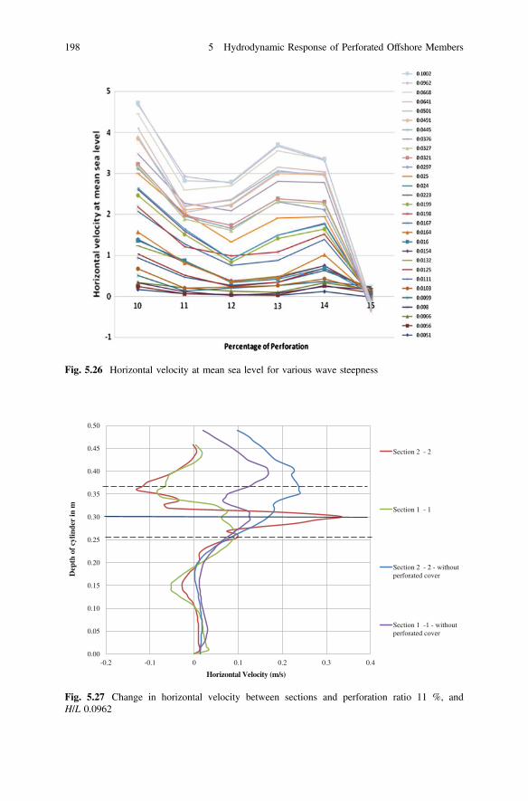
Fig. 5.26 Horizontal velocity at mean sea level for various wave steepness
0.00
0.05
0.10
0.15
0.20
0.25
0.30
0.35
0.40
0.45
0.50
-0.2 -0.1 0 0.1 0.2 0.3 0.4
Dep
th o
f cy
linde
r in
m
Horizontal Velocity (m/s)
Section 2 - 2
Section 1 - 1
Section 2 - 2 - without perforated cover
Section 1 -1 - without perforated cover
Fig. 5.27 Change in horizontal velocity between sections and perforation ratio 11 %, andH/L 0.0962
198 5 Hydrodynamic Response of Perforated Offshore Members
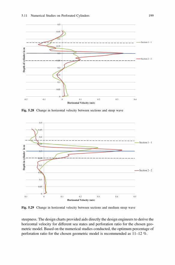
steepness. The design charts provided aids directly the design engineers to derive thehorizontal velocity for different sea states and perforation ratio for the chosen geo-metric model. Based on the numerical studies conducted, the optimum percentage ofperforation ratio for the chosen geometric model is recommended as 11–12 %.
0
0.05
0.1
0.15
0.2
0.25
0.3
0.35
0.4
0.45
0.5
-0.2 -0.1 0 0.1 0.2 0.3 0.4
Dep
th o
f cy
linde
r in
m
Horizontal Velocity (m/s)
Section 1 - 1
Section 2 - 2
Fig. 5.28 Change in horizontal velocity between sections and steep wave
0
0.05
0.1
0.15
0.2
0.25
0.3
0.35
0.4
0.45
0.5
-0.1 0 0.1 0.2 0.3 0.4 0.5
Dep
th in
cyl
inde
r in
m
Horizontal Velocity (m/s)
Section 1 - 1
Section 2 - 2
Fig. 5.29 Change in horizontal velocity between sections and medium steep wave
5.11 Numerical Studies on Perforated Cylinders 199
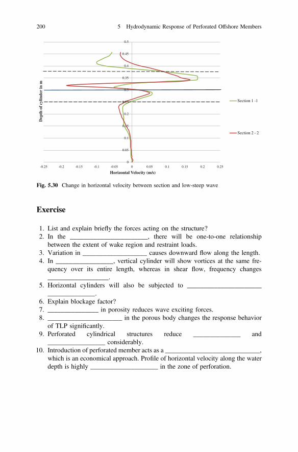
Exercise
1. List and explain briefly the forces acting on the structure?2. In the _______________________, there will be one-to-one relationship
between the extent of wake region and restraint loads.3. Variation in ___________________ causes downward flow along the length.4. In _________________, vertical cylinder will show vortices at the same fre-
quency over its entire length, whereas in shear flow, frequency changes__________________.
5. Horizontal cylinders will also be subjected to ____________________________________.
6. Explain blockage factor?7. _______________ in porosity reduces wave exciting forces.8. ______________________ in the porous body changes the response behavior
of TLP significantly.9. Perforated cylindrical structures reduce ______________ and
_________________ considerably.10. Introduction of perforated member acts as a ____________________________,
which is an economical approach. Profile of horizontal velocity along the waterdepth is highly ____________________ in the zone of perforation.
0
0.05
0.1
0.15
0.2
0.25
0.3
0.35
0.4
0.45
0.5
-0.25 -0.2 -0.15 -0.1 -0.05 0 0.05 0.1 0.15 0.2 0.25
Dep
th o
f cy
linde
r in
m
Horizontal Velocity (m/s)
Section 1 -1
Section 2 - 2
Fig. 5.30 Change in horizontal velocity between section and low-steep wave
200 5 Hydrodynamic Response of Perforated Offshore Members

Answers
1. Forces acting on the structures in fluid medium shall be classified as drag(acting in-line with the direction of flow) and lift (transverse to the direction offlow). Further, drag force can be classified as higher and smaller frequencycomponents. These components will be functions of the geometry of thestructure and flow conditions. Lift forces contain oscillatory components withmultiple frequencies. On the downstream side, flow will return to its unalteredcondition. This is due to fluid viscosity and damping. The region of altered flowdirectly behind the structure is called wake region.
2. Wake regions.3. Stagnation pressure.4. Uniform flow; continuously.5. Flow-induced vibrations.6. Closely spaced members, connected in different orientations, cause distortion in
the fluid field around them. For closely spaced members, the structure becomesdense. For dense structures, flow field slows down as it travels through thestructure. This causes blockage effect and complicates the actual velocity fieldaround the structure. Load on the structure increases due to this blockage.
7. Increase.8. Drag force.9. Wave–structure interaction and scouring problems.
10. Good energy dissipation technique; Nonlinear.
Answers 201
Chapter 6Introduction to Stochastic Dynamics
Abstract This chapter deals with introduction to stochastic dynamics and itsapplication to offshore structures. This chapter introduces the basics of reliabilityapproach to the ultimate load design, levels of reliability, methods of reliability,reliability estimates, and limitation. The limitations and advantages of stochasticmodels are also explained. A quick preview about FOSM and advanced FOSM isalso given in this chapter. Introduction to fatigue and fracture assessment is alsoprovided.
Keywords Stochastic dynamics � Ultimate load � Reliability � FOSM � AdvancedFOSM � Offshore structures
6.1 Introduction
In most of the cases, offshore structures are exposed to the environmental loads thatcan be modeled as a piecewise stationary process. A stationary process is one forwhich the statistical properties such as mean value and standard deviation are samefor all points in time (or) position. Hence, the following equation holds good:
mx ¼ E X tð Þ½ � ¼ constant ð6:1Þ
For the condition mx = mx(t) to be satisfied, autocorrelation function is given by:
RXðsÞ ¼ E½XðtÞXðt þ sÞ� to remain function of s only ð6:2Þ
To check whether the following are independent of time:
m̂xðtÞ ¼ 1N
XNj¼1
xjðtÞ ð6:3Þ
© Springer India 2015S. Chandrasekaran, Dynamic Analysis and Design of Offshore Structures,Ocean Engineering & Oceanography 5, DOI 10.1007/978-81-322-2277-4_6
203
R̂xðt; t þ sÞ ¼ 1N
XNj¼1
xjðtÞxjðt þ sÞ ð6:4Þ
If they remain independent of time, the process is said to be a stationary process.Stationary process is defined by satisfying the condition given in Eq. (6.1):
The auto-covariance function should be as follows:
CXðsÞ ¼ E½ðXðtÞ � mxÞðXðt þ sÞ � mxÞ� ¼ function of s only ð6:5Þ
For a stationary process, transfer between the load and the response can bemodeled as linear, time-invariant, while the system can be characterized by atransfer function. Hence, the relationship between variance spectrum of theresponse (called response spectrum) and variance spectrum of load (called loadspectrum) is determined by a transfer function.
Let F(t) denote a stochastic load process. Assuming that F(t) acts as a linear,time-invariant system, which has an impulse response function hFX(t), for eachrealization f(t) of F(t), we get the corresponding realization x(t) of the response X(t).Hence,
xðtÞ ¼Z1�1
hFXðsÞ f ðt � sÞds
¼Z10
hFXðsÞ f ðt � sÞds
because hFXðsÞ ¼ 0 for s\0
ð6:6Þ
Equation (6.6) establishes the connection between the realization of the loadprocess and the corresponding realization of the response process. This connectioncan also be described as below:
XðtÞ ¼Z10
hFXðsÞFðt � sÞds ð6:7Þ
The above equation interprets that there exists a relation between all the cor-responding pairs of realization of F(t) and X(t). It is important to note that theimpulse response function or the transfer function, which determines the connectionbetween the load and the response, is completely defined by the properties of thelinear system. This remains independent of any given load. In the term of hFX(t),index FX is to be understood only as the visual indicator for the connection betweenF(t) and X(t). For example, if Y(t) is the response of the load process G(t), acting onthe same linear system, then hGY(t) = hFX(t).
204 6 Introduction to Stochastic Dynamics
6.1.1 Mean Value of the Response Process
Assuming that f1(t),…, fN(t) is the sequence of realization of F(t), let x1(t),…, xN(t),which denotes the corresponding response realization, then
1N
XNj¼1
xjðtÞ ¼ 1N
XNj¼1
Z10
hFXðsÞfjðt � sÞds ð6:8Þ
¼Z10
hFXðsÞ1N
XNj¼1
Z10
fjðt � sÞds8<:
9=; ð6:9Þ
This leads to the following relationship:
E½XðtÞ� ¼ limN!1
1N
XNj¼1
xjðtÞ ¼Z10
hFXðsÞ limN!1
1N
XNj¼1
fjðt � sÞ( )
ds ð6:10Þ
¼Z10
hFXðsÞE½Fðt � sÞ� ds ð6:11Þ
If F(t) is a stationary process, then mF = E[F(t)] is a constant. Then,
E½XðtÞ� ¼ mF
Z10
hFXðsÞds ð6:12Þ
It can be seen that the above equation is independent of time. Hence,
mX ¼ E X tð Þ½ � ¼ constant ð6:13Þ
Let HFXðxÞ be the transfer function that corresponds to the impulse responsefunction of hFX(t). Then,
HFXð0Þ ¼Z10
hFXðsÞds
E½XðtÞ� ¼ mFHFXð0Þ ¼ mX
ð6:14Þ
6.1 Introduction 205
For the system, whose equation of motion is given by:
m€uþ c _uþ ku ¼ P0 cosðxtÞ ð6:15Þ
The transfer function for the linear system, described by the above equation ofmotion, is given by HFXðxÞ. For the steady-state response of the system under thegiven excitation load, the dynamic amplification factor D is given by:
D ¼ 1ffiffiffiffiffiffiffiffiffiffiffiffiffiffiffiffiffiffiffiffiffiffiffiffiffiffiffiffiffiffiffiffiffiffiffiffiffiffið1� b2Þ2 þ ð2nbÞ2
q ð6:16Þ
For a weakly damped system, we also know that the maximum amplificationfactor is given by:
Dmax ¼ 12n
ð6:17Þ
For ξ = 2 %,Dmax = 25, which implies that, even small oscillating forces may leadto large responses. For the analysis of structural response to various forcing fre-quencies, it is therefore better to introduce a complex-valued function as given below:
HðxÞ ¼ HðxÞj je�iu
uðtÞ ¼ HðxÞj jP0 cosðxt � uÞ ð6:18Þ
In the above equation, HðxÞ gives the amplitude amplification and ϕ gives thephase shift. For example, if HðxÞ ¼ 0:001, for a particular frequency x, then aforce amplitude of 100 N will give rise to the displacement of 0.1 m at thisfrequency. The generalized expression for the steady-state response of the oscil-lating system is given by:
upðtÞ ¼ q cosðxt � uÞq
xstatic¼ q
P0=K
� � ¼ D
Hence,
upðtÞ ¼ P0
K1ffiffiffiffiffiffiffiffiffiffiffiffiffiffiffiffiffiffiffiffiffiffiffiffiffiffiffiffiffiffiffiffiffiffiffiffiffiffi
ð1� b2Þ2 þ ð2nbÞ2q cosðxt � uÞ
ð6:19Þ
Comparing Eqs. (6.18) and (6.19), we get
HðxÞ ¼ 1K
1ffiffiffiffiffiffiffiffiffiffiffiffiffiffiffiffiffiffiffiffiffiffiffiffiffiffiffiffiffiffiffiffiffiffiffiffiffiffið1� b2Þ2 þ ð2nbÞ2
q ð6:20Þ
206 6 Introduction to Stochastic Dynamics
where HðxÞ is called the transfer function or frequency response function, whichmaps the response behavior of the linear system to the external forcing function. Itis seen that this function is proportional to the dynamic amplification factor. Itcontains all relevant information about the dynamic amplification. Incorporatingalso the information related to the phase shift, transfer function is modified as:
HðxÞ ¼ 1K
1ffiffiffiffiffiffiffiffiffiffiffiffiffiffiffiffiffiffiffiffiffiffiffiffiffiffiffiffiffiffiffiffiffiffiffiffiffiffið1� b2Þ2 þ ð2nbÞ2
q e�iu ð6:21Þ
The reason, why it is easier to use e�i/, in comparison to sinϕ or cosϕ is that
ddtðeiuÞ ¼ i
dudt
ðeiuÞ; where eiu factor does not changeeiu1eiu2 ¼ eiðu1þu2Þ ¼ eiu3 ; where the product of two factors are of the same kind:
The above two properties give many advantages in the derivations. Further,HFX(0) = (1/k) and mX = (mF/K). This means that the mean value of the response isequal to the product of the mean value of the load and the system response to astatic load of unit size; hence, the following equation holds good:
mX ¼ HFXð0ÞmF ð6:22Þ
It is seen from the above equation that, for the excitation force with zero meanvalue, response also has zero mean value.
6.2 Auto-Covariance of the Response Process
It is seen from the above section that for mF = 0, mX is also zero. Hence, for F(t) tobe a stationary process, it is convenient to assume F′(t) = F(t) − mF, which also haszero mean value. Let X′(t) be the response to the load process, F′(t). Then,
X 0ðtÞ ¼Z10
hFXðsÞ F0ðt � sÞ ds
¼Z10
hFXðsÞFðt � sÞds�Z10
hFXðsÞ mF ds
¼ XðtÞ � mX ð6:23Þ
6.1 Introduction 207
For X′(t) to have a zero mean value, F(t) and F′(t) have the same auto-covariance.Then, the following relation holds good:
xjðtÞxjðt þ sÞ ¼Z10
hFXðs1Þ fjðt � s1Þ ds1�Z10
hFXðs2Þ fjðt þ s� s2Þds2
¼Z10
Z10
hFXðs1ÞhFXðs2Þ fjðt � s1Þ fjðt þ s� s2Þds1ds2 ð6:24Þ
It is also known that:
E½XðtÞXðt þ sÞ� ¼ limN!1
1N
XNj¼1
xjðtÞxjðt þ sÞ ð6:25Þ
Hence, Eq. (6.24) can be rewritten as:
¼Z10
Z10
hFXðs1ÞhFXðs2Þ limN!1
1N
XNj¼1
fjðt � s1Þfjðt þ s� s2Þds1ds2
¼Z10
Z10
hFXðs1ÞhFXðs2ÞE½Fðt � s1ÞFðt þ s� s2Þ�ds1ds2
¼Z10
Z10
hFXðs1ÞhFXðs2ÞCFðsþ s1 � s2Þds1ds2
ð6:26Þ
Since F(t) is assumed to be stationary, E½XðtÞXðt þ sÞ� will also be independentof time. The auto-covariance CX(τ) will be as same as the auto-correlation RX(τ), asthe process is a zero mean process. Then, the following relation holds good:
CXðsÞ ¼Z10
Z10
hFXðs1ÞhFXðs2ÞCFðsþ s1 þ s2Þds1ds2: ð6:27Þ
6.3 Response Spectrum
Let SX(ω) be the variance spectrum of the response of the process X(t) and SF(ω) bethe variance spectrum of the load process F(t), then variance spectrum of X(t) willbe defined by the Fourier transform of the auto-covariance of the response, which isgiven by
208 6 Introduction to Stochastic Dynamics
SXðxÞ ¼ 12p
Z1�1
CXðsÞe�ixsds
SXðxÞ ¼Z10
hFXðs1Þ
Z10
hFXðs2Þ12p
Z1�1
CFðsþ s1 � s2Þe�ixsdsds2ds1
Put sþ s1 � s2 ¼ h; dh ¼ ds; then
SXðxÞ ¼Z10
hFXðs1Þ
Z10
hFXðs2Þ12p
Z1�1
CFðhÞe�ixhdheixðs1�s2Þds2ds1
ð6:28Þ
SXðxÞ ¼ HFXð�xÞHFXðxÞSFðxÞ because eð�ixÞ� ¼ eix and hFXðtÞ is a real function.Imposing the above condition, we get:
HFXð�xÞ ¼Z10
hFXðtÞeixtdt ¼Z10
hFXðtÞe�ixt�dt
Z10
hFXðtÞe�ixt�dt ¼ HFXðxÞ�
SXðxÞ ¼ HFXðxÞj j2SFðxÞ
ð6:29Þ
The above equation gives the relationship between the response spectrum SXðxÞand the load spectrum SFðxÞ. Please note that Eq. (6.29) does not contain infor-mation about the phase shift between the load and the response; only amplitudeamplification is known. From the response spectrum, one can compute several otherstatistical quantities that are important for assessing the response. For example,standard deviation of the response is obtained as follows:
mX ¼ HFXð0ÞmF
r2X ¼Z1�1
HFXðxÞj j2SFðxÞdxð6:30Þ
For X(t) be the response of a linear system with transfer function HFXðxÞ to astationary load process F(t), RHS of the Eq. (6.30) for standard deviation is to becomputed numerically. For very less damping, HFXðxÞj j2 becomes narrow aroundthe resonance frequency, xr. This implies that the main contribution to the integralEq. (6.30) comes from a small interval around xr, which is evident from theFig. 6.1.
If SF(ω) varies much slower than that of HFXðxÞj j2, then it is often possible toreplace SF(ω) in Eq. (6.30) by S0 = SF(ωr). Hence, Eq. (6.30) can be rewritten as
6.3 Response Spectrum 209
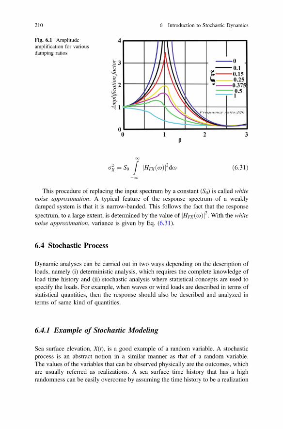
r2X ¼ S0
Z1�1
HFXðxÞj j2dx ð6:31Þ
This procedure of replacing the input spectrum by a constant (S0) is called whitenoise approximation. A typical feature of the response spectrum of a weaklydamped system is that it is narrow-banded. This follows the fact that the responsespectrum, to a large extent, is determined by the value of HFXðxÞj j2. With the whitenoise approximation, variance is given by Eq. (6.31).
6.4 Stochastic Process
Dynamic analyses can be carried out in two ways depending on the description ofloads, namely (i) deterministic analysis, which requires the complete knowledge ofload time history and (ii) stochastic analysis where statistical concepts are used tospecify the loads. For example, when waves or wind loads are described in terms ofstatistical quantities, then the response should also be described and analyzed interms of same kind of quantities.
6.4.1 Example of Stochastic Modeling
Sea surface elevation, X(t), is a good example of a random variable. A stochasticprocess is an abstract notion in a similar manner as that of a random variable.The values of the variables that can be observed physically are the outcomes, whichare usually referred as realizations. A sea surface time history that has a highrandomness can be easily overcome by assuming the time history to be a realization
Fig. 6.1 Amplitudeamplification for variousdamping ratios
210 6 Introduction to Stochastic Dynamics
of ergodic stationary process. The assumption implies that the statistical informa-tion about the process is in fact contained in a single realization of the process. Forexample, cumulative distribution function (CDF) FX(t)(x) assumes the values lesserthan or equal to x, as given below:
FXðtÞðxÞ ¼ limT!1
T½xðtÞ� x�T
where T denotes the record length and T ½xðtÞ� x� denotes the total amount of timeduring T where ½xðtÞ� x�. The quantity X(t) is called as a stochastic process if X(t) isa random variable for each value of t in an interval (a, b).
6.4.2 Example of a Stochastic Process
Assume X as a random variable, which is normally distributed with a mean valuem and standard deviation σ (>0). Its probability density function is given by:
fXðxÞ ¼ 1ffiffiffiffiffiffi2p
prexp � 1
2x� mr
h i2� �
If g(t) is known, which is a real function defined for (−∞ < t < ∞), then
g tð Þ ¼ cosðxtÞ
where ω is a positive constant. Hence, X(t) = Xg(t) is also a stochastic processdefined for the same interval (−∞ < t <∞). Realization of the process is then givenas a product of g(t) with an outcome x of the random variable X. In that case, thefollowing equation holds good:
xðtÞ ¼ xgðtÞ
Hence, if g(t) = cos(ωt); its realization could be harmonic function of the sameperiod, but with a different amplitude. Hence, the mean value is given by:
mXðtÞ ¼ E X g tð Þ½ � ¼ E X½ �g tð Þ ¼ mg tð ÞrXðtÞ ¼
ffiffiffiffiffiffiffiffiffiffiffiffiffiffiffiffiffiffiffiffiffiffiffiffiffiffiffiffiffiffiffiffiffiffiffiffiffiffiffiE½X gðtÞ2 � mgðtÞ2�
q¼
ffiffiffiffiffiffiffiffiffiffiffiffiffiffiffiffiffiffiffiffiffiffiffiffiffiffiffiffiffiffiffiffiffiffiffiffiffiffiffiffiffiE½X2�gðtÞ2 � m2gðtÞ2
q¼
ffiffiffiffiffiffiffiffiffiffiffiffiffiffiffiffiffiffiffiffiffiffiffiffiffiffiffiffiffiffiffiffiffiE½X2 � m2 gðtÞj j�
p¼ r gðtÞj j
6.4 Stochastic Process 211
For each value of t, g(t) is a constant; Hence X(t) = Xg(t) is also normallydistributed if g tð Þ 6¼ 0
The probability density function of X(t) becomes:
f XðtÞðxÞ ¼ 1ffiffiffiffiffiffi2p
pr gðtÞj j exp � 1
2x� mgðtÞr gðtÞj j
� �2( )
:
6.5 Return Period
Let Z be a random variable. Then,
p ¼ Prob Z[ z½ � ¼ 1� FZ zð Þ ð6:32Þ
Assuming that we can make series of observations of Z, mean number ofobservations to the first observed or measured value of X exceeds z is called thereturn period for exceedance of z, which is denoted by �RðzÞ.
�RðzÞ ¼ 1p¼ 1
1� FZðzÞ ð6:33Þ
This equation can be described as an average of (1/p) trails conducted before anevent of probability p occurs. �RðzÞ refers to the number of observations, and theseare assumed to be statistically independent. If return period needs to be explained interms of time, one needs to know the time interval between the observations. If theobservation interval is Dt, then the return period, in terms of time, is given by:
RðzÞ ¼ Dt �RðzÞ ð6:34Þ
The observation interval must be chosen sufficiently long such that individualobservations become approximately independent. For example, a design load with aprobability of 10−2 being exceeded during 1 year is often used in offshore struc-tures. If we let F(t) denote the relevant load process considered for the design and ξdenote the corresponding load level, then
ProbðZ[ nÞ ¼ 0:01; where Z ¼ max ðFðtÞÞ; 0� tÞ� 1 year:
Return period of exceedance of ξ then becomes as follows:
�RðzÞ ¼ 1ProbðZ[ nÞ ¼
10:01
¼ 100 years ð6:35Þ
212 6 Introduction to Stochastic Dynamics
Reference period, in this case, is 1 year, and therefore, return period ofexceedance is 100 years. It is important to note that the time-varying loads, causedby waves, cannot be considered stationary over an extended period. This means thatthe quantities such as yearly maxima must be computed using long-term statistics.Return periods are also computed based on the risk associated. This is a commonpractice in case of earthquake loads and seismic design of structures. For example,design basis earthquake (DBE) has a risk level of 10 % at occurrence of 50 yearsand that of maximum credible earthquake (MCE) is 2 %. Based on the risk asso-ciated, return period is computed as below:
R ¼ 1� 1� 1T
n
For DBE, 0:1 ¼ 1� 1� 1T
50yields return period ðTÞ as 475 years
ForMCE, 0:02 ¼ 1� 1� 1T
50yields a retrun period of 2;500 years:
ð6:36Þ
6.6 Safety and Reliability
Safety is a measure used to indicate the reliability. But this demands a traditionalway of analysis. Reliability offers probabilistic meaning to this traditional concept.Extension of reliability analysis also includes the consequences of failure. Safetyassessment and risk characterization are vital for offshore plants. Since risk is therealization of hazard and hazard scenario is unavoidable in any process industry, themost important aspect of reliability is to account for all uncertainties that makethe structure vulnerable to failure under a pre-defined limit state. Accuracy of thereliability studies depends on how accurately these uncertainties are accounted forin the analysis. Many assumptions are made during the reliability analyses, whichinfluence the accuracy of the reliability studies. Furthermore, it is also important tonote that analytical formulation of the limit state surface and integration of theprobability density function within the domain of interest is also very complex.
6.7 Reliability Framework
In the general sense, offshore platform should perform its intended function for aspecified period of time under specific conditions. In the mathematical sense ornarrow sense, reliability is estimating the probability of the structure for notattaining the limit state of collapse within the specified conditions, for the specifiedperiod of time.
6.5 Return Period 213
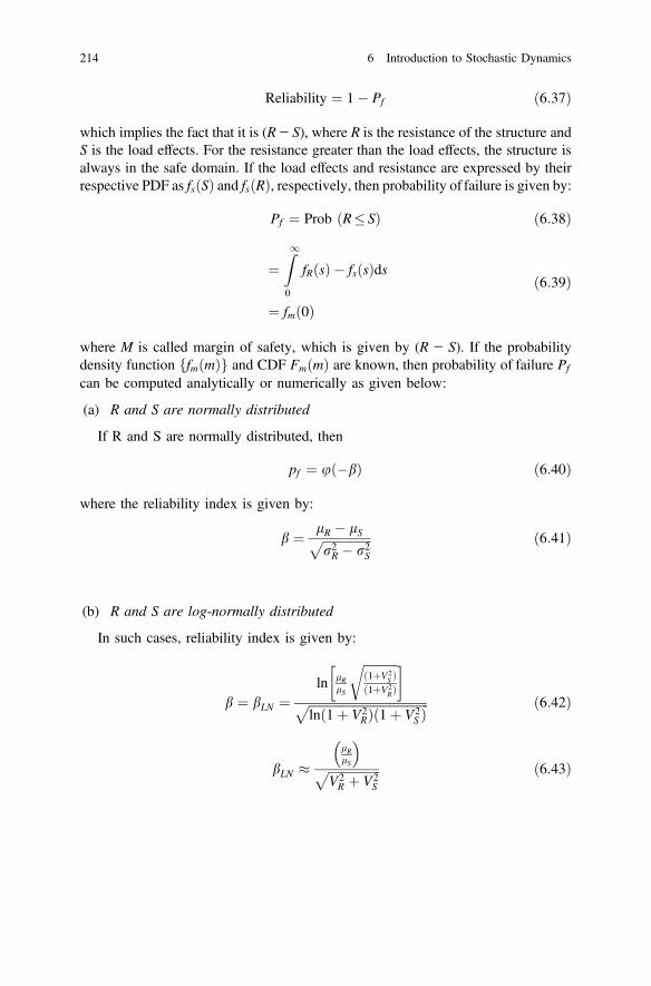
Reliability ¼ 1� Pf ð6:37Þ
which implies the fact that it is (R − S), where R is the resistance of the structure andS is the load effects. For the resistance greater than the load effects, the structure isalways in the safe domain. If the load effects and resistance are expressed by theirrespective PDF as fsðSÞ and fsðRÞ, respectively, then probability of failure is given by:
Pf ¼ Prob ðR� SÞ ð6:38Þ
¼Z10
fRðsÞ � fsðsÞds
¼ fmð0Þð6:39Þ
where M is called margin of safety, which is given by (R − S). If the probabilitydensity function ffmðmÞg and CDF FmðmÞ are known, then probability of failure Pf
can be computed analytically or numerically as given below:
(a) R and S are normally distributed
If R and S are normally distributed, then
pf ¼ u �bð Þ ð6:40Þ
where the reliability index is given by:
b ¼ lR � lSffiffiffiffiffiffiffiffiffiffiffiffiffiffiffiffir2R � r2S
p ð6:41Þ
(b) R and S are log-normally distributed
In such cases, reliability index is given by:
b ¼ bLN ¼ln lR
lS
ffiffiffiffiffiffiffiffiffiffiffið1þV2
S Þð1þV2
RÞ
r ffiffiffiffiffiffiffiffiffiffiffiffiffiffiffiffiffiffiffiffiffiffiffiffiffiffiffiffiffiffiffiffiffiffiffiffiffiffiffilnð1þ V2
RÞð1þ V2S Þ
p ð6:42Þ
bLN �lRlS
� �ffiffiffiffiffiffiffiffiffiffiffiffiffiffiffiffiffiV2R þ V2
S
p ð6:43Þ
214 6 Introduction to Stochastic Dynamics
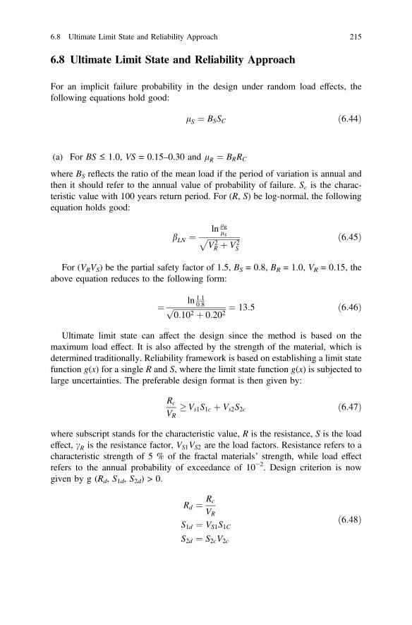
6.8 Ultimate Limit State and Reliability Approach
For an implicit failure probability in the design under random load effects, thefollowing equations hold good:
lS ¼ BSSC ð6:44Þ
(a) For BS ≤ 1.0, VS = 0.15–0.30 and lR ¼ BRRC
where BS reflects the ratio of the mean load if the period of variation is annual andthen it should refer to the annual value of probability of failure. Sc is the charac-teristic value with 100 years return period. For (R, S) be log-normal, the followingequation holds good:
bLN ¼ln lR
lSffiffiffiffiffiffiffiffiffiffiffiffiffiffiffiffiffiV2R þ V2
S
p ð6:45Þ
For (VRVS) be the partial safety factor of 1.5, BS = 0.8, BR = 1.0, VR = 0.15, theabove equation reduces to the following form:
¼ ln 1:10:8ffiffiffiffiffiffiffiffiffiffiffiffiffiffiffiffiffiffiffiffiffiffiffiffiffiffiffi
0:102 þ 0:202p ¼ 13:5 ð6:46Þ
Ultimate limit state can affect the design since the method is based on themaximum load effect. It is also affected by the strength of the material, which isdetermined traditionally. Reliability framework is based on establishing a limit statefunction g(x) for a single R and S, where the limit state function g(x) is subjected tolarge uncertainties. The preferable design format is then given by:
Rc
VR�Vs1S1c þ Vs2S2c ð6:47Þ
where subscript stands for the characteristic value, R is the resistance, S is the loadeffect, cR is the resistance factor, VS1VS2 are the load factors. Resistance refers to acharacteristic strength of 5 % of the fractal materials’ strength, while load effectrefers to the annual probability of exceedance of 10−2. Design criterion is nowgiven by g (Rd, S1d, S2d) > 0.
Rd ¼ Rc
VR
S1d ¼ VS1S1CS2d ¼ S2cV2c
ð6:48Þ
6.8 Ultimate Limit State and Reliability Approach 215
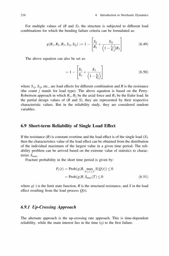
For multiple values of (R and S), the structure is subjected to different loadcombinations for which the bending failure criteria can be formulated as:
gðR1;R2;R3; S1j; S2jÞ :¼ 1� SijR1
þ S2j
1� S1jR2
� �R3
24
35 ð6:49Þ
The above equation can also be set as:
¼ 1� X1
X1þ X3
1� X1R4
� �24
35 ð6:50Þ
where S1j, S2j, etc., are load effects for different combination and R is the resistance(the count j stands for load type). The above equation is based on the Perry-Robertson approach in which R1, R2 be the axial force and R3 be the Euler load. Inthe partial design values of (R and S), they are represented by their respectivecharacteristic values. But in the reliability study, they are considered randomvariables.
6.9 Short-term Reliability of Single Load Effect
If the resistance (R) is constant overtime and the load effect is of the single load (S),then the characteristics value of the load effect can be obtained from the distributionof the individual maximum of the largest value in a given time period. The reli-ability problem can be arrived based on the extreme value of statistics to charac-terize Smax.
Fracture probability in the short time period is given by:
Pf ðtÞ ¼ ProbðgðR; max0� t� T
SðQðtÞÞ� 0
¼ ProbðgðR; Smax Tð Þ� 0 ð6:51Þ
where g(·) is the limit state function, R is the structural resistance, and S in the loadeffect resulting from the load process Q(t).
6.9.1 Up-Crossing Approach
The alternate approach is the up-crossing rate approach. This is time-dependentreliability, while the main interest lies in the time (tf) to the first failure.
216 6 Introduction to Stochastic Dynamics
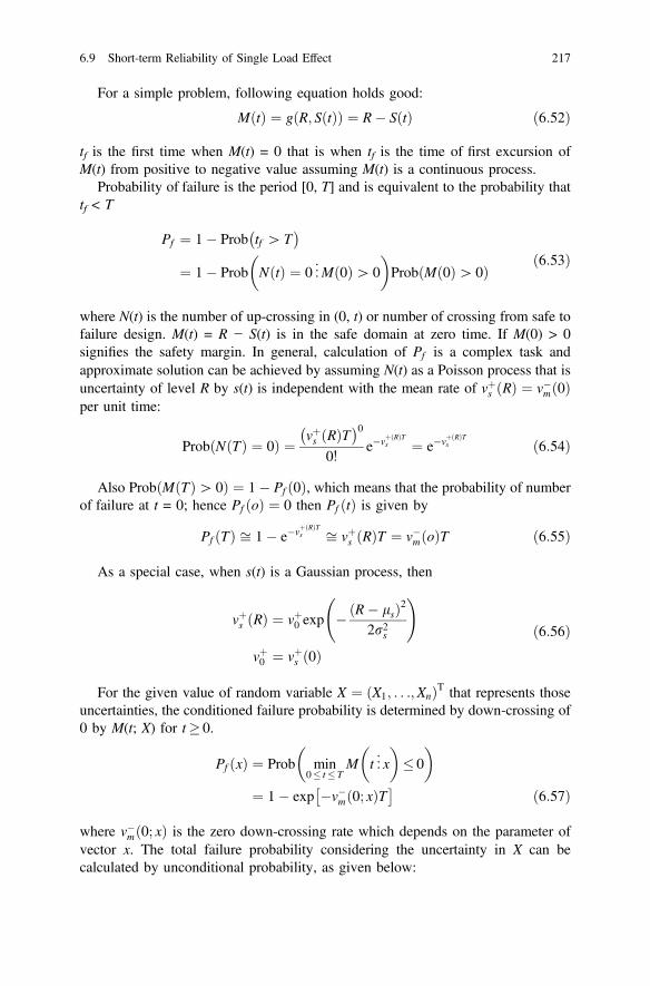
For a simple problem, following equation holds good:
MðtÞ ¼ g R; SðtÞð Þ ¼ R� SðtÞ ð6:52Þ
tf is the first time when M(t) = 0 that is when tf is the time of first excursion ofM(t) from positive to negative value assuming M(t) is a continuous process.
Probability of failure is the period [0, T] and is equivalent to the probability thattf < T
Pf ¼ 1� Prob tf [ T� �
¼ 1� Prob N tð Þ ¼ 0 ...M 0ð Þ[ 0
� �Prob M 0ð Þ[ 0ð Þ ð6:53Þ
where N(t) is the number of up-crossing in (0, t) or number of crossing from safe tofailure design. M(t) = R − S(t) is in the safe domain at zero time. If M(0) > 0signifies the safety margin. In general, calculation of Pf is a complex task andapproximate solution can be achieved by assuming N(t) as a Poisson process that isuncertainty of level R by s(t) is independent with the mean rate of vþs Rð Þ ¼ v�m 0ð Þper unit time:
Prob N Tð Þ ¼ 0ð Þ ¼ vþs Rð ÞT� �00!
e�vþ Rð ÞTs ¼ e�vþ Rð ÞT
s ð6:54Þ
Also Prob M Tð Þ[ 0ð Þ ¼ 1� Pf ð0Þ, which means that the probability of numberof failure at t = 0; hence Pf oð Þ ¼ 0 then Pf ðtÞ is given by
Pf Tð Þ ffi 1� e�vþ Rð ÞTs ffi vþs Rð ÞT ¼ v�m oð ÞT ð6:55Þ
As a special case, when s(t) is a Gaussian process, then
vþs Rð Þ ¼ vþ0 exp �ðR� lsÞ22r2s
!
vþ0 ¼ vþs 0ð Þð6:56Þ
For the given value of random variable X ¼ ðX1; . . .;XnÞT that represents thoseuncertainties, the conditioned failure probability is determined by down-crossing of0 by M(t; X) for t� 0.
Pf xð Þ ¼ Prob min0� t�T
M t ...x
� �� 0
� �¼ 1� exp �v�m 0; xð ÞT � ð6:57Þ
where v�m 0; xð Þ is the zero down-crossing rate which depends on the parameter ofvector x. The total failure probability considering the uncertainty in X can becalculated by unconditional probability, as given below:
6.9 Short-term Reliability of Single Load Effect 217
Pf ¼Zx
Pf xð Þfx xð Þdx ð6:58Þ
The integral represents expected value of Pf ðxÞ. Hence, Pf can be calculated as arandom value, as shown below:
Pf ffi 1N
XNi¼1
Pf ðxiÞ: ð6:59Þ
6.10 Long-term Reliability of Single Load Effect
For a non-stationary process M(t; x) which could be for a long-term, failureprobability is given by:
Pf xð Þ ¼ 1� exp �ZT0
v�m 0; t; xð Þdt8<:
9=; ð6:60Þ
where v�m 0; t; xð Þ is the mean down-crossing rate which depends as the sea state andchanges with time. For the given set of properties of the sea states, let W be thecaptured value, which is given by
W ¼ Hs;Tp; uc; uw;wave*
;wind*
; current*
� �
where Hs is the significant wave height, Tp spectral peak period, uc current velocity,
uw mean wave speed, and wave*
;wind*
; current*
are wave, wind, current direction.Pre-requisite of the long-term failure probability is to impose an ergodicityassumption on the environmental process W = W(t), then
Pf xð Þ ¼ 1� exp �TZw
v�m 0;w; xð Þfx wð Þdw8<:
9=; ð6:61Þ
where v�m 0;w; xð Þ derives mean zero down-crossing rate of M for the sea stateW = w:
fw wð Þ ¼ PDF ofW ð6:62Þ
218 6 Introduction to Stochastic Dynamics
The full long-term failure probability occurring for both environment variabilityand parameter uncertainty is given by:
Pf ¼Zx
Pf xð Þfx xð Þdx: ð6:63Þ
6.11 Levels of Reliability
Reliability studies are considered in different levels in the literature. Level I isfocusing on the probability aspects of the problem. Suitable characteristic values ofthe random variables are introduced in the safety analysis. Main objective of thislevel of study is to minimize the deviation of the design values from that of thetarget value. For example, load-resistance factor design (LRFD) is of level I ofreliability. Level II has two values for each parameter to be defined in the analysis,namely mean and standard deviation. Level III is a complete analysis of theproblem addressing the multi-dimensional probability density function of randomvariables, which is extended over the safety domain. Reliability is expressed interms of suitable safety indices. In level IV, engineering economics is also appliedin the reliability study. This level of reliability study is usually applied to structuresof strategic importance. The study includes cost-benefit analysis, rehabilitation,consequence of failure, and return on capital investment.
Reliability methods offer many advantages: (i) they account for the uncertainties;(ii) they are rational methods to estimate safety; and (iii) they offer decision-makingsupport for non-economic and better balanced design. Optimal distribution ofmaterial among various components of structure can be benefitted through a con-stant update mechanism, on the basis of which FEED function of engineeringjudgment are circumscribed. Reliability studies expand the knowledge of uncer-tainties in the response of the structure. There are few obstacles in implementing thereliability studies to the offshore plants in operation. They are classified as inertial,cultural, and philosophical. Different types of variables used in reliability studyare, namely (i) elementary variables (static variables) like material properties,(ii) geometry of the platform, (iii) boundary conditions, and (iv) issues related to thelocation and behavior dependent data.
Failure modes such as limit stress and limit displacement depend upon thesystem variables, which are in turn dependent on location behavior and failuremodes. There are different steps of reliability, namely elementary level, componentlevel, system level, and detailed field investigation. The first step is handled bystochastic modeling, while the second step can be handled by probabilistic study offailure of components. In case of system-level studies, probabilistic studies on thefailure of the whole system can be investigated. One of the serious limitations ofreliability study is that it requires a large amount of data on the failure scenario.Other parameters that influence the accuracy of the results of the reliability studiesare as follows:
6.10 Long-term Reliability of Single Load Effect 219
1. Separation of two variables, namely safety domain and failure domain.2. Nature of variables, namely external or internal and whether they are inde-
pendent or not.3. Effect of time indicating the static content or the cyclic (dynamic) content.4. Form of the performance function, which is dependent on the physical model of
the system.
6.12 Reliability Methods
The main interest is to develop a reliability method in relation to modeling thematerials and structures. The primary advantage of the reliability method instructures is to calculate the reliability estimates by nominal or conditional prob-ability; reliability index; serviceability of failure to stochastic date description.Three fields of application are particularly targeted; they are as follows:
1. Exceptionally highly innovative structures for which experience accumulated inlast few certainties are inadequate. Reliability methods were first used fordesigning offshore platform.
2. Design of ordinary-type structures with codes whose current evolutions offerpossibility of calibration of partial coefficients using reliability methods.
3. Monitoring of structures during the life span so that repair strategies can beoptimized through reliability.
6.12.1 Advantages of Reliability Methods (ASC-83)
The advantages of reliability methods are as listed below
• Offer a realistic procession of uncertainties and the methods for evaluating thesafety factors that are often too arbitrary.
• Offer decision-making support for more economic and better balanced design.• Analyze failure modes and measure the reliability provided by application and
regulations.• Allow the optimal distribution of material and arrange various components of
the structure.• Benefit from the experience acquired in design by updating on the basis of
feedback from the experience.• Expand the knowledge of uncertainty in response to the structure.
There are some obstacles in the implementation of these advantages. They are asfollows:
220 6 Introduction to Stochastic Dynamics
• These methods demand new approach and call to our thinking and workingpattern.
• Because it is more of a probabilistic approach and lesser statistical approach, itdemands more mathematical concepts rather than engineering skills.
• They explicitly underscore the acceptance of risk, and using safety coefficients,they demand the judgment and decision.
• One should have minimum statistical knowledge of elementary properties ofvariables, and we need to use these in modeling.
6.13 Stochastic Models
The stochastic modeling essentially helps to establish variability by best-suitedprobability density function. They can be done by two approaches, namely natu-ralist’s approach and physicist’s approach. Reliability is also an observation of thesample that estimates μ, SD, and variance. This often gives ad hoc estimates orestimates by interval. These estimates are themselves a random variable, sincebased on this best judgment, PDF has to be determined. Alternatively, as per thephysicist’s approach, this seeks to understand the variability of the material’sbehavior on a microscopic scale. Results of reliability calculation depend on thequantity of data. But these data are always insufficient due to limitations that arisefrom the size of test samples, infinite domain, and distribution trails. Reliabilityanalysis also requires failure scenario, which separates the situation that thedesigner decides as acceptable from those of the other. Complexities of reliabilityare mainly due to the nature of the random variables, effect of time, mechanicalmodels and the form of performance function chosen for the analysis.
6.13.1 First-Order Second-Moment Method (FOSM)
In this case, first-order Taylor series approximation of the limit stat function is usedfor the analysis. Only second moments of the random variables are used to estimatethe probability of failure. Limit state function is defined as:
M ¼ R� S ð6:64Þ
where R and S are statistically independent and assumed to be normally distributed.Hence, following relationship holds good:
lm ¼ lR � lS ð6:65Þ
rm ¼ rR2 þ rS2 ð6:66Þ
6.12 Reliability Methods 221
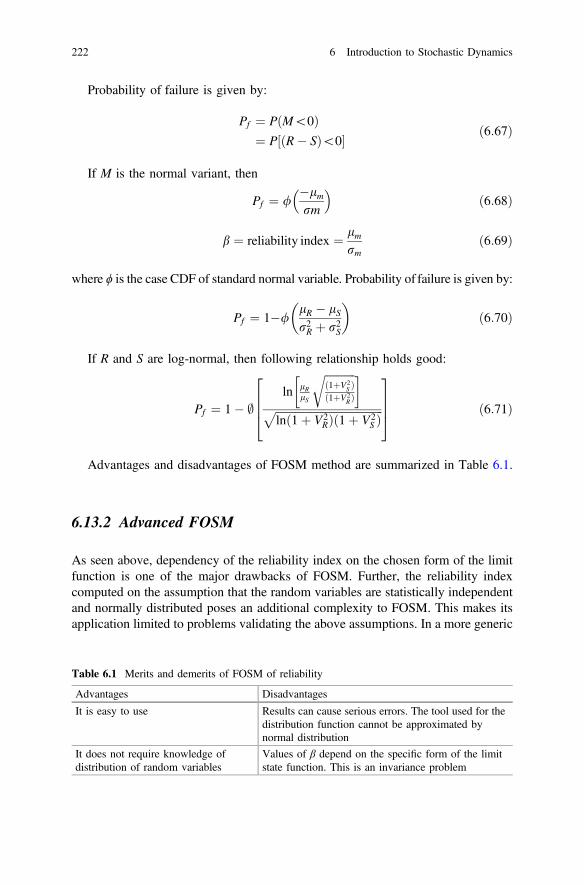
Probability of failure is given by:
Pf ¼ P M\0ð Þ¼ P R� Sð Þ\0½ � ð6:67Þ
If M is the normal variant, then
Pf ¼ /�lmrm
� �ð6:68Þ
b ¼ reliability index ¼ lmrm
ð6:69Þ
where ϕ is the case CDF of standard normal variable. Probability of failure is given by:
Pf ¼ 1�/lR � lSr2R þ r2S
� �ð6:70Þ
If R and S are log-normal, then following relationship holds good:
Pf ¼ 1� ;ln lR
lS
ffiffiffiffiffiffiffiffiffiffiffið1þV2
S Þð1þV2
RÞ
r ffiffiffiffiffiffiffiffiffiffiffiffiffiffiffiffiffiffiffiffiffiffiffiffiffiffiffiffiffiffiffiffiffiffiffiffiffiffiffilnð1þ V2
RÞð1þ V2S Þ
p2664
3775 ð6:71Þ
Advantages and disadvantages of FOSM method are summarized in Table 6.1.
6.13.2 Advanced FOSM
As seen above, dependency of the reliability index on the chosen form of the limitfunction is one of the major drawbacks of FOSM. Further, the reliability indexcomputed on the assumption that the random variables are statistically independentand normally distributed poses an additional complexity to FOSM. This makes itsapplication limited to problems validating the above assumptions. In a more generic
Table 6.1 Merits and demerits of FOSM of reliability
Advantages Disadvantages
It is easy to use Results can cause serious errors. The tool used for thedistribution function cannot be approximated bynormal distribution
It does not require knowledge ofdistribution of random variables
Values of β depend on the specific form of the limitstate function. This is an invariance problem
222 6 Introduction to Stochastic Dynamics
form, advanced FOSM gives reliability index; Hasofer Lind method is one of theadvanced FOSMs, which is discussed below.
The key point of the method is to estimate a design point, which is the minimumdistance of failure from the origin. The minimum distance is the safety index (βHL).The method actually transforms the random variable into a reduced form, which canbe given as:
Xi ¼ xi � xirxi
for i ¼ 1; 2; . . .; nf g ð6:72Þ
This reduced variable will have a zero mean and unit standard deviation, whichis a special process of distribution. Hence, the performance function G(x) = 0 isconverted into G(x′) = 0 to enable the mapping between the required domains.Reliability index βHL is given by:
bHL ¼ffiffiffiffiffiffiffiffiffixdxTd
qð6:73Þ
where xd is the minimum distance of the design point from the origin, which is alsoreferred as a check point.
Following cases are specific:
Case 1: Limit state function is linear
Let us considerM ¼ R� S ð6:74Þ
The reduced values are computed for the domain mapping, as discussed below:
R ¼ R� lRrR
ð6:75Þ
S ¼ S� lSrS
ð6:76Þ
M ¼ ðrR þ lRÞ � ðrS þ lSÞ ð6:77Þ
As the limit state function moves closer to the origin, failure region is mapped.Reliability index is given by:
b ¼ lR � lSffiffiffiffiffiffiffiffiffiffiffiffiffiffiffiffiffiffiffir2R þ Rr2R
p ð6:78Þ
6.13 Stochastic Models 223
Case 2: Limit state function is nonlinear
In such cases, computing the minimum distance for calculating the reliability indexactually becomes an optimization problem.
bHL ¼ D ¼ pxð Þt xð Þ ð6:79Þ
The above function is to be minimized subject to the condition that G(x) = 0 formany random variables (x1, x2,…, xn), which originates from the safe state of thedomain; G(x) < 0 indicates failure. Hence G(x) > 0 denotes the minimum distancefrom the origin to a point on the limit state function, which is called design point.The problem is now reduced to determining the coordinates of the design point,geometrically or analytically. By this definition, reliability index becomes invariantas the minimum distance remains constant regardless of the shape of the limit statefunction. Using the Lagrange multipliers, one can find the minimum distance asgiven below:
bHL ¼ �Pni¼1 x
0di
@G@0xdiffiffiffiffiffiffiffiffiffiffiffiffiffiffiffiffiffiffiffiffiffiffiffiffiffiPn
i¼1@G@Xdi
� �2r ð6:80Þ
where @G@Xdi
is the partial derivative, evaluated at the design point with coordinates(xdi, xd2, …).
6.14 Fatigue and Fracture
Fatigue design of marine structures requires a description of long-term variation oflocal stress caused by wave action, variable buoyancy, slamming, and vortexshedding. Main contribution to fatigue damage is caused by the frequency of loadoccurring that are of the order of 10–20 % of that of extreme load effects in theservice life. Fatigue failures are catastrophic as they come without warning andcause significant damage. Physical process of fatigue consists of initiation of crack,stable crack growth, and unstable crack growth until rupture. Once the crack isinitiated, it will tend to grow in a direction orthogonal to the direction of theoscillatory tensile stresses. Fatigue is a challenging failure mode to deal withbecause the initiation process of fatigue is unpredictable; difficulties exist in map-ping the studies carried out in the lab scale to real structures. Fatigue failure iscontrolled by the following: (i) design, material, and structural detailing to addressthe probability of crack initiation; (ii) regular inspection during construction andoperation; and (iii) following repair procedures as advised by the design loads. Incase of design, the limiting conditions are already defined in advance, which are
224 6 Introduction to Stochastic Dynamics
referred as limit states. This will include the case of failure at some defined extremeloads, which will include fatigue life requirements. Commonly checked limit statefor marine structures are strength under extreme loading, fatigue life, fracture, anddeflection. It is a common practice to present the results of strength, fatigue, andfracture as unity check.
Let U ¼ actual or factored loadAcceptable load which is used for strength check.
For fatigue, the unity check is U ¼ ffiffiffiffiffiffiffiffiffiffiffiffiffiffiffiffiffiffiffiffiffiffiffiffiffiffiffiffiffiffiffiffiffiffiffiffiffiffiffiffiDesign life damagem
pwhere
m ¼ �slope�1 of S–Ncurve:
6.15 Fatigue Assessment
When the steel member is subjected to large fluctuating tensile stress, small cracksdevelop; these cracks grow in size and further progress, which make the structure tobreak. For machinery design where the stress fluctuation is similar throughout thedesign life, cyclic stresses are kept below the endurance limit. But for structures,this method is not permissible as the mixture of large-amplitude and small-ampli-tude stresses occur due to environmental loads. Hence, it becomes necessary todesign the structures for intended fatigue life. Common design approach is nothingbut the usage of S–N curve. These curves are based on experiments conducted ondifferent types of structures. Fatigue failure can be detected by the occurrence ofvisible cracks, thickness of the crack, and complete loss of load-carrying capacity.
6.15.1 SN Approach
Test on the steel specimen subjected to fluctuating loading showed that the numberof cycles to failure (N) is inversely proportional to the stress range that is maximumand minimum stress, let it will be S, which is the power of m:
N / 1sm
N ¼ ASm�1
If measures are taken to prevent corrosion, then for constant amplitude of stresscycling there is a cutoff stress below which no fatigue occurs. This is found to be2 × 108 cycles. For variable amplitude stress cycling, which is the most general casewith the marine structures, the cutoff value of stress decreases as the fatigue crackgrows. The slope of S–N curve changes beyond 107 cycles from m to m + 2. Thiseffect is significant if one is looking for the higher order of fatigue lives. Hence, forpreliminary analysis, S–N curve can be taken as linear, which often simplifies the
6.14 Fatigue and Fracture 225
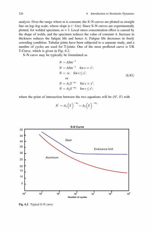
analysis. Over the range where m is constant, the S–N curves are plotted as straightline on log–log scale, whose slope is (−1/m). Since S–N curves are experimentallyplotted, for welded specimen, m = 3. Local stress concentration effect is caused bythe shape of welds, and the specimen reduces the value of constant A. Increase inthickness reduces the fatigue life and hence A. Fatigue life decreases in freelycorroding condition. Tubular joints have been subjected to a separate study, and anumber of cycles are used for T-joints. One of the most proffered curve is UKT-Curve, which is given in Fig. 6.2.
S–N curve may be typically be formulated as
N ¼ ASm�1
N ¼ ASm�1 for s[ s0;N ¼ 1 for s� s0;
or
N ¼ A1S�m1 for s[ s0;
N ¼ A2S�m2 for s� s0;
ð6:81Þ
where the point of intersection between the two equations will be (N′, S′) with
N0 ¼ A1 S
0� ��m1¼ A2 S
0� ��m2
103 104 105 10
6 10
7 10
8 10
9
Number of cycles
5
15
25
35
45
10
20
30
40
50
Aluminium
Steel
Endurance limit
S-N Curve
Fig. 6.2 Typical S–N curve
226 6 Introduction to Stochastic Dynamics
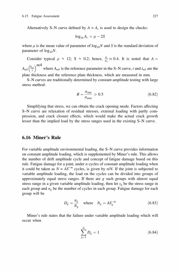
Alternatively S–N curve defined by A = Ac is used to design the checks:
log10 Ac ¼ l� 2S
where μ is the mean value of parameter of log10N and S is the standard deviation ofparameter of log10N.
Consider typical μ ≈ 12; S ≈ 0.2; hence, AclA
� 0:4. It is noted that A ¼
Areftreft
� �m=4where Aref is the reference parameter in the S–N curve, t and tref are the
plate thickness and the reference plate thickness, which are measured in mm.S–N curves are traditionally determined by constant amplitude testing with large
stress method:
R ¼ rmin
rmax[ 0:5 ð6:82Þ
Simplifying that stress, we can obtain the crack opening mode. Factors affectingS–N curve are relaxation of residual stresses, external loading with partly com-pression, and crack closure effects, which would make the actual crack growthlesser than the implied load by the stress ranges used in the existing S–N curve.
6.16 Miner’s Rule
For variable amplitude environmental loading, the S–N curve provides informationon constant amplitude loading, which is supplemented by Miner’s rule. This allowsthe number of drift amplitude cycle and concept of fatigue damage based on thisrule. Fatigue damage for a joint, under n cycles of constant amplitude loading whenit could be taken as N = AS−m cycles, is given by n/N. If the joint is subjected tovariable amplitude loading, the load on the cycles can be divided into groups ofapproximately equal stress ranges. If there are g such groups with almost equalstress range in a given variable amplitude loading, then let sg be the stress range ineach group and ng be the number of cycles in each group. Fatigue damage for eachgroup will be
Dg ¼ ngNg
where Ng ¼ AS�mg ð6:83Þ
Miner’s rule states that the failure under variable amplitude loading which willoccur when
XGg¼1
Dg ¼ 1 ð6:84Þ
6.15 Fatigue Assessment 227
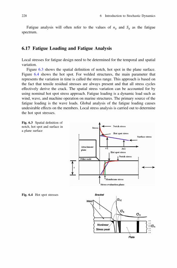
Fatigue analysis will often refer to the values of ng and Sg as the fatiguespectrum.
6.17 Fatigue Loading and Fatigue Analysis
Local stresses for fatigue design need to be determined for the temporal and spatialvariation.
Figure 6.3 shows the spatial definition of notch, hot spot in the plane surface.Figure 6.4 shows the hot spot. For welded structures, the main parameter thatrepresents the variation in time is called the stress range. This approach is based onthe fact that tensile residual stresses are always present and that all stress cycleseffectively derive the crack. The spatial stress variation can be accounted for byusing nominal hot spot stress approach. Fatigue loading is a dynamic load such aswind, wave, and machine operation on marine structures. The primary source of thefatigue loading is the wave loads. Global analysis of the fatigue loading causesundesirable effects on the members. Local stress analysis is carried out to determinethe hot spot stresses.
Fig. 6.3 Spatial definition ofnotch, hot spot and surface ina plane surface
Fig. 6.4 Hot spot stresses
228 6 Introduction to Stochastic Dynamics
6.18 Time Domain Fatigue Analysis
Time domain fatigue analysis results in time series of stress. For narrowbandGaussian response, the cycles are well defined. For more general stress time his-tories, cycle counting methods have to be applied to all types of response timeseries. Time domain methods use only the information provided by the series ofpeaks (local maximum) and valleys (local minima). According to different methodsof constructing the effective stress ranges from these identified peaks and valleys,various cycle counting methods are used. The procedures are described by ASTM-1985. This includes peak counting, range counting, level-crossing counting, andrain flow counting. Among these, rain flow counting is the best for fatigue damageestimates.
6.18.1 Rain Flow Counting
This method was first proposed by Matsuishi and Endo (1968). Let us consider astress time series of peaks and valleys with the time axis vertically downwards.Lines connecting peaks and valley from a series of pagoda roofs are constructed.Each rain flow begins at the beginning of the time series at the inside every peakand valley. Rain flow initiating at a peak (or a valley) drop down until it reachespeak more positive (or a valley, more negative) than the peak (or the valley) fromwhere it started. Rain flow also stops when it meets the rain flow roof assume. Rainflow must terminate at the end of the time series. Horizontal length of each rain flowis counted as half-cycle with that stress range.
6.18.1.1 Methodology
1. Reduce the time history to a sequence of (tensile) peaks and (compressive)troughs.
2. Imagine that the time history is a pagoda.3. Turn the sheet clockwise 90°, so the starting time is at the top.4. Each tensile peak is imagined as a source of water that ‘drips’ down the pagoda.5. Count the number of half-cycles by looking for terminations in the flow
occurring when:
• it reaches the end of the time history;• it merges with a flow that started at an earlier tensile peak; or• it encounters a trough of greater magnitude.
6. Repeat Step 5 for compressive troughs.7. Assign a magnitude to each half-cycle equal to the stress difference between its
start and termination.
6.18 Time Domain Fatigue Analysis 229
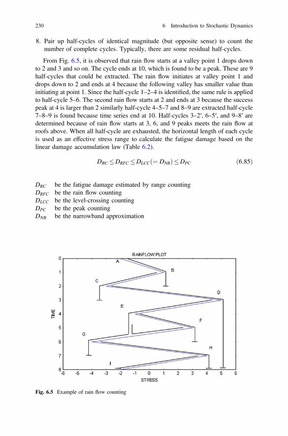
8. Pair up half-cycles of identical magnitude (but opposite sense) to count thenumber of complete cycles. Typically, there are some residual half-cycles.
From Fig. 6.5, it is observed that rain flow starts at a valley point 1 drops downto 2 and 3 and so on. The cycle ends at 10, which is found to be a peak. These are 9half-cycles that could be extracted. The rain flow initiates at valley point 1 anddrops down to 2 and ends at 4 because the following valley has smaller value thaninitiating at point 1. Since the half-cycle 1–2–4 is identified, the same rule is appliedto half-cycle 5–6. The second rain flow starts at 2 and ends at 3 because the successpeak at 4 is larger than 2 similarly half-cycle 4–5–7 and 8–9 are extracted half-cycle7–8–9 is found because time series end at 10. Half-cycles 3–2′, 6–5′, and 9–8′ aredetermined because of rain flow starts at 3, 6, and 9 peaks meets the rain flow atroofs above. When all half-cycle are exhausted, the horizontal length of each cycleis used as an effective stress range to calculate the fatigue damage based on thelinear damage accumulation law (Table 6.2).
DRC �DRFC �DLCC ¼ DNBð Þ�DPC ð6:85Þ
DRC be the fatigue damage estimated by range countingDRFC be the rain flow countingDLCC be the level-crossing countingDPC be the peak countingDNB be the narrowband approximation
Fig. 6.5 Example of rain flow counting
230 6 Introduction to Stochastic Dynamics
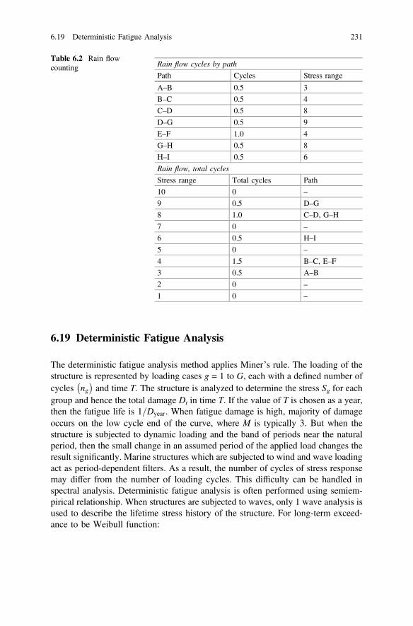
6.19 Deterministic Fatigue Analysis
The deterministic fatigue analysis method applies Miner’s rule. The loading of thestructure is represented by loading cases g = 1 to G, each with a defined number ofcycles ng
� �and time T. The structure is analyzed to determine the stress Sg for each
group and hence the total damage Dt in time T. If the value of T is chosen as a year,then the fatigue life is 1=Dyear. When fatigue damage is high, majority of damageoccurs on the low cycle end of the curve, where M is typically 3. But when thestructure is subjected to dynamic loading and the band of periods near the naturalperiod, then the small change in an assumed period of the applied load changes theresult significantly. Marine structures which are subjected to wind and wave loadingact as period-dependent filters. As a result, the number of cycles of stress responsemay differ from the number of loading cycles. This difficulty can be handled inspectral analysis. Deterministic fatigue analysis is often performed using semiem-pirical relationship. When structures are subjected to waves, only 1 wave analysis isused to describe the lifetime stress history of the structure. For long-term exceed-ance to be Weibull function:
Table 6.2 Rain flowcounting Rain flow cycles by path
Path Cycles Stress range
A–B 0.5 3
B–C 0.5 4
C–D 0.5 8
D–G 0.5 9
E–F 1.0 4
G–H 0.5 8
H–I 0.5 6
Rain flow, total cycles
Stress range Total cycles Path
10 0 –
9 0.5 D–G
8 1.0 C–D, G–H
7 0 –
6 0.5 H–I
5 0 –
4 1.5 B–C, E–F
3 0.5 A–B
2 0 –
1 0 –
6.19 Deterministic Fatigue Analysis 231
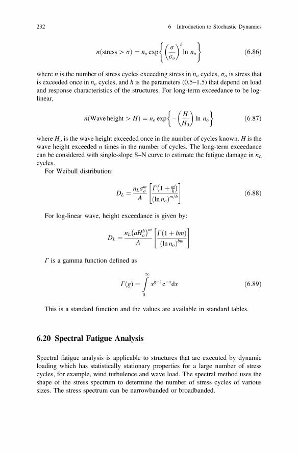
n stress[ rð Þ ¼ no exprro
� �h
ln no
( )ð6:86Þ
where n is the number of stress cycles exceeding stress in no cycles, ro is stress thatis exceeded once in no cycles, and h is the parameters (0.5–1.5) that depend on loadand response characteristics of the structures. For long-term exceedance to be log-linear,
n Wave height[Hð Þ ¼ no exp � HH0
� �ln no
� �ð6:87Þ
where Ho is the wave height exceeded once in the number of cycles known. H is thewave height exceeded n times in the number of cycles. The long-term exceedancecan be considered with single-slope S–N curve to estimate the fatigue damage in nLcycles.
For Weibull distribution:
DL ¼ nLrmoA
C 1þ mh
� �ln noð Þm=h
" #ð6:88Þ
For log-linear wave, height exceedance is given by:
DL ¼ nL aHbo
� �mA
C 1þ bmð Þln noð Þbm
" #
Γ is a gamma function defined as
Cðg) ¼Z10
xg�1e�xdx ð6:89Þ
This is a standard function and the values are available in standard tables.
6.20 Spectral Fatigue Analysis
Spectral fatigue analysis is applicable to structures that are executed by dynamicloading which has statistically stationary properties for a large number of stresscycles, for example, wind turbulence and wave load. The spectral method uses theshape of the stress spectrum to determine the number of stress cycles of varioussizes. The stress spectrum can be narrowbanded or broadbanded.
232 6 Introduction to Stochastic Dynamics
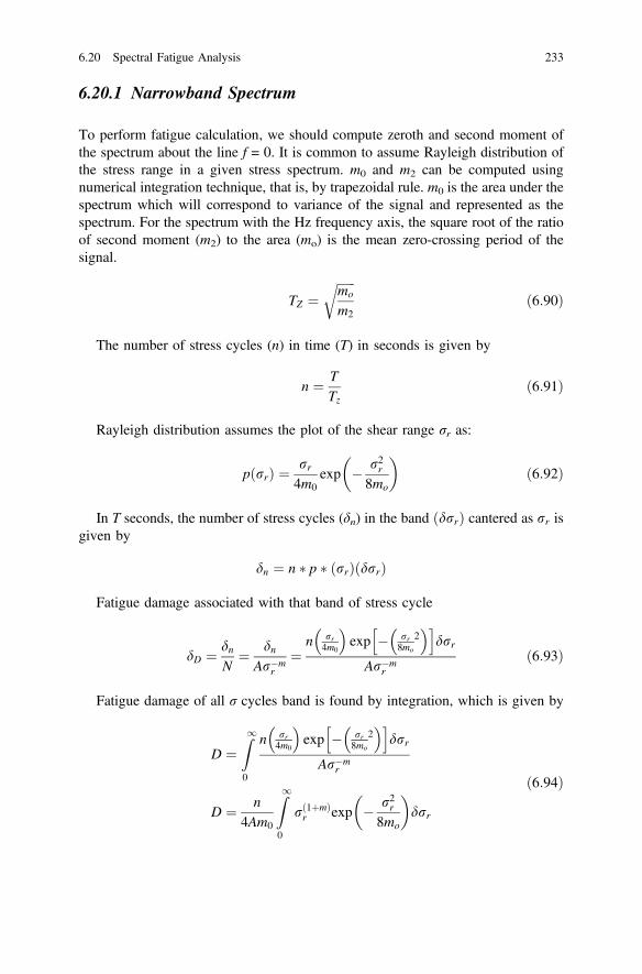
6.20.1 Narrowband Spectrum
To perform fatigue calculation, we should compute zeroth and second moment ofthe spectrum about the line f = 0. It is common to assume Rayleigh distribution ofthe stress range in a given stress spectrum. m0 and m2 can be computed usingnumerical integration technique, that is, by trapezoidal rule. m0 is the area under thespectrum which will correspond to variance of the signal and represented as thespectrum. For the spectrum with the Hz frequency axis, the square root of the ratioof second moment (m2) to the area (mo) is the mean zero-crossing period of thesignal.
TZ ¼ffiffiffiffiffiffimo
m2
rð6:90Þ
The number of stress cycles (n) in time (T) in seconds is given by
n ¼ TTz
ð6:91Þ
Rayleigh distribution assumes the plot of the shear range σr as:
p rrð Þ ¼ rr4m0
exp � r2r8mo
� �ð6:92Þ
In T seconds, the number of stress cycles (δn) in the band ðdrrÞ cantered as rr isgiven by
dn ¼ n � p � ðrrÞ drrð Þ
Fatigue damage associated with that band of stress cycle
dD ¼ dnN
¼ dnAr�m
r¼
n rr4m0
� �exp � rr
8mo
2� �h i
drr
Ar�mr
ð6:93Þ
Fatigue damage of all σ cycles band is found by integration, which is given by
D ¼Z10
n rr4m0
� �exp � rr
8mo
2� �h i
drr
Ar�mr
D ¼ n4Am0
Z10
rð1þmÞr exp � r2r
8mo
� �drr
ð6:94Þ
6.20 Spectral Fatigue Analysis 233
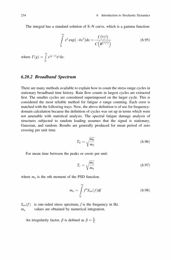
The integral has a standard solution of S–N curve, which is a gamma function:
Z10
xa exp �bx2� �
dx ¼ C aþ1c
� �C B
aþ1cð Þ� � ð6:95Þ
where C gð Þ ¼ R10xðg�1Þexdx:
6.20.2 Broadband Spectrum
There are many methods available to explain how to count the stress range cycles instationary broadband time history. Rain flow counts in largest cycles are extractedfirst. The smaller cycles are considered superimposed on the larger cycle. This isconsidered the most reliable method for fatigue σ range counting. Each crest ismatched with the following trays. Now, the above definition is of use for frequency-domain calculation because the definition of cycles was set up in terms which werenot amenable with statistical analysis. The spectral fatigue damage analysis ofstructures subjected to random loading assumes that the signal is stationary,Gaussian, and random. Results are generally produced for mean period of zerocrossing per unit time.
TZ ¼ffiffiffiffiffiffim0
m2
rð6:96Þ
For mean time between the peaks or crests per unit:
Tc ¼ffiffiffiffiffiffim2
m4
rð6:97Þ
where mn is the nth moment of the PSD function.
mn ¼Z10
f nSrr fð Þdf ð6:98Þ
Srrðf Þ is one-sided stress spectrum, f is the frequency in Hz.mn values are obtained by numerical integration.
An irregularity factor, β is defined as b ¼ TcTz
234 6 Introduction to Stochastic Dynamics
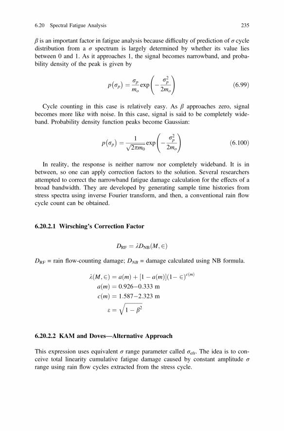
β is an important factor in fatigue analysis because difficulty of prediction of σ cycledistribution from a σ spectrum is largely determined by whether its value liesbetween 0 and 1. As it approaches 1, the signal becomes narrowband, and proba-bility density of the peak is given by
p rp� � ¼ rp
moexp � r2p
2mo
!ð6:99Þ
Cycle counting in this case is relatively easy. As β approaches zero, signalbecomes more like with noise. In this case, signal is said to be completely wide-band. Probability density function peaks become Gaussian:
p rp� � ¼ 1ffiffiffiffiffiffiffiffiffiffiffi
2pm0p exp � r2p
2mo
!ð6:100Þ
In reality, the response is neither narrow nor completely wideband. It is inbetween, so one can apply correction factors to the solution. Several researchersattempted to correct the narrowband fatigue damage calculation for the effects of abroad bandwidth. They are developed by generating sample time histories fromstress spectra using inverse Fourier transform, and then, a conventional rain flowcycle count can be obtained.
6.20.2.1 Wirsching’s Correction Factor
DRF ¼ kDNBðM;2Þ
DRF = rain flow-counting damage; DNB = damage calculated using NB formula.
k M;2ð Þ ¼ a mð Þ þ 1� a mð Þ½ �ð1� 2ÞcðmÞa mð Þ ¼ 0:926�0:333 m
c mð Þ ¼ 1:587�2:323 m
e ¼ffiffiffiffiffiffiffiffiffiffiffiffiffi1� b2
q
6.20.2.2 KAM and Doves—Alternative Approach
This expression uses equivalent σ range parameter called σefr. The idea is to con-ceive total linearity cumulative fatigue damage caused by constant amplitude σrange using rain flow cycles extracted from the stress cycle.
6.20 Spectral Fatigue Analysis 235
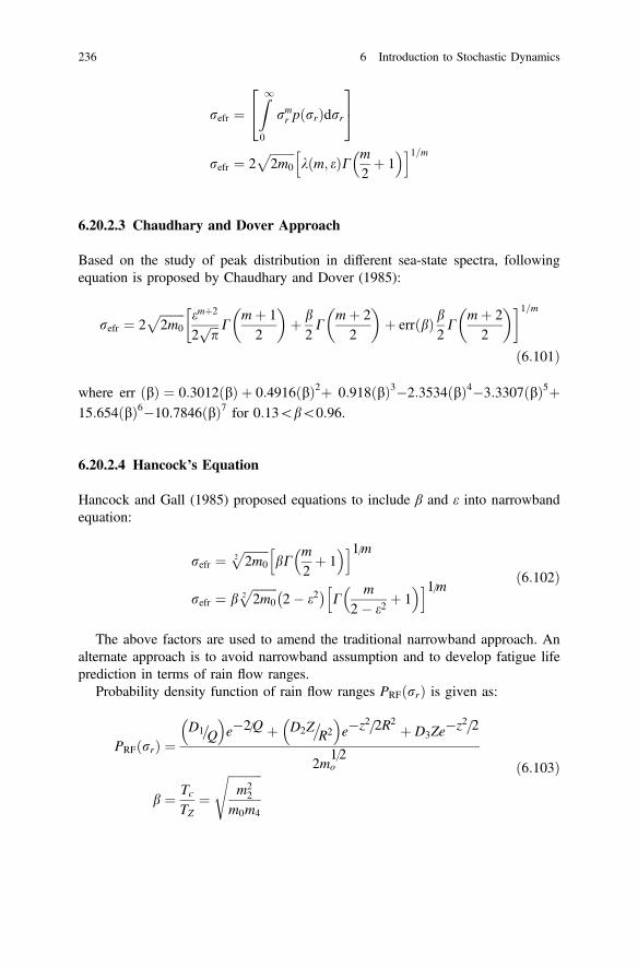
refr ¼Z10
rmr p rrð Þdrr24
35
refr ¼ 2ffiffiffiffiffiffiffiffi2m0
pkðm; eÞC m
2þ 1
� �h i1=m
6.20.2.3 Chaudhary and Dover Approach
Based on the study of peak distribution in different sea-state spectra, followingequation is proposed by Chaudhary and Dover (1985):
refr ¼ 2ffiffiffiffiffiffiffiffi2m0
p emþ2
2ffiffiffip
p Cmþ 12
� �þ b
2C
mþ 22
� �þ err bð Þ b
2C
mþ 22
� � 1=mð6:101Þ
where err bð Þ ¼ 0:3012 bð Þ þ 0:4916 bð Þ2þ 0:918 bð Þ3�2:3534 bð Þ4�3:3307 bð Þ5þ15:654 bð Þ6�10:7846 bð Þ7 for 0:13\b\0:96.
6.20.2.4 Hancock’s Equation
Hancock and Gall (1985) proposed equations to include β and ε into narrowbandequation:
refr ¼ffiffiffiffiffiffiffiffi2m0
2p
bCm2þ 1
� �h i1=mrefr ¼ b
ffiffiffiffiffiffiffiffi2m0
2p
2� e2� �
Cm
2� e2þ 1
� �h i1=m ð6:102Þ
The above factors are used to amend the traditional narrowband approach. Analternate approach is to avoid narrowband assumption and to develop fatigue lifeprediction in terms of rain flow ranges.
Probability density function of rain flow ranges PRF rrð Þ is given as:
PRF rrð Þ ¼D1=Q
� �e�2=Q þ D2Z
�R2
� �e�z2=2R2 þ D3Ze
�z2=2
2m1=2o
b ¼ TcTZ
¼ffiffiffiffiffiffiffiffiffiffiffim2
2
m0m4
s ð6:103Þ
236 6 Introduction to Stochastic Dynamics
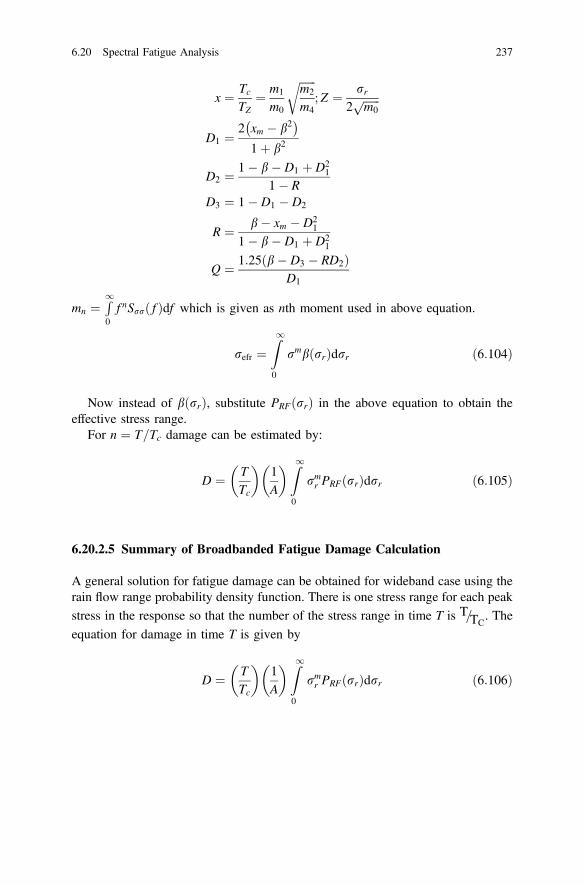
x ¼ TcTZ
¼ m1
m0
ffiffiffiffiffiffim2
m4
r; Z ¼ rr
2ffiffiffiffiffiffim0
p
D1 ¼2 xm � b2� �1þ b2
D2 ¼ 1� b� D1 þ D21
1� RD3 ¼ 1� D1 � D2
R ¼ b� xm � D21
1� b� D1 þ D21
Q ¼ 1:25 b� D3 � RD2ð ÞD1
mn ¼R10f nSrr fð Þdf which is given as nth moment used in above equation.
refr ¼Z10
rmb rrð Þdrr ð6:104Þ
Now instead of b rrð Þ, substitute PRF rrð Þ in the above equation to obtain theeffective stress range.
For n ¼ T=Tc damage can be estimated by:
D ¼ TTc
� �1A
� �Z10
rmr PRF rrð Þdrr ð6:105Þ
6.20.2.5 Summary of Broadbanded Fatigue Damage Calculation
A general solution for fatigue damage can be obtained for wideband case using therain flow range probability density function. There is one stress range for each peakstress in the response so that the number of the stress range in time T is T=TC
. Theequation for damage in time T is given by
D ¼ TTc
� �1A
� �Z10
rmr PRF rrð Þdrr ð6:106Þ
6.20 Spectral Fatigue Analysis 237
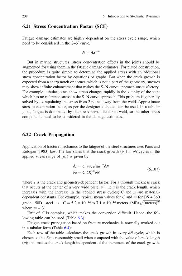
6.21 Stress Concentration Factor (SCF)
Fatigue damage estimates are highly dependent on the stress cycle range, whichneed to be considered in the S–N curve.
N ¼ AS�m
But in marine structures, stress concentration effects in the joints should beaugmented for using them in the fatigue damage estimates. For plated construction,the procedure is quite simple to determine the applied stress with an additionalstress concentration factor by equations or graphs. But when the crack growth isexpected from a sharp notch or corner, which is not a part of the geometry, stressesmay show infinite enhancement that makes the S–N curve approach unsatisfactory.For example, tubular joints show stress changes rapidly in the vicinity of the jointwhich has no reference stress in the S–N curve approach. This problem is generallysolved by extrapolating the stress from 2 points away from the weld. Approximatestress concentration factor, as per the designer’s choice, can be used. In a tubularjoint, fatigue is dominated by the stress perpendicular to weld, so the other stresscomponents need to be considered in the damage estimates.
6.22 Crack Propagation
Application of fracture mechanics to the fatigue of the steel structures uses Paris andErdogan (1983) law. The law states that the crack growth dað Þ in δN cycles in theapplied stress range of rrð Þ is given by
da ¼ C yrrffiffiffiffiffiffipa
p �mdN
da ¼ C dK½ �mdN ð6:107Þ
where y is the crack and geometry-dependent factor. For a through thickness crackthat occurs at the center of a very wide plate, y = 1; a is the crack length, whichincreases with the increase in the applied stress cycles; C and m are material-dependent constants. For example, typical mean values for C and m for BS 4,360grade 50D steel is C ¼ 5:2 10�12 to 7:1 10�12 meters =MPa
ffiffiffiffiffiffiffiffiffiffiffiffiffiffiffiffiffiffiffiffimetersð Þm
pwhere m = 3.
Unit of C is complex, which makes the conversion difficult. Hence, the fol-lowing table can be used (Table 6.3).
Fatigue crack propagation based on fracture mechanics is normally worked outin a tabular form (Table 6.4):
Each row of the table calculates the crack growth in every δN cycle, which ischosen so that δa is reasonably small when compared with the value of crack length(a); this makes the crack length independent of the increment of the crack growth.
238 6 Introduction to Stochastic Dynamics
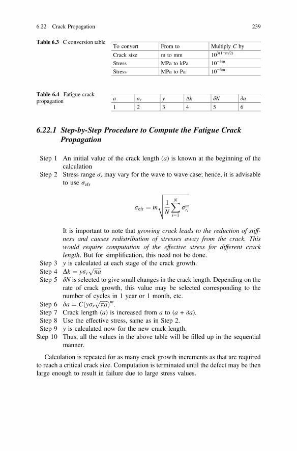
6.22.1 Step-by-Step Procedure to Compute the Fatigue CrackPropagation
Step 1 An initial value of the crack length (a) is known at the beginning of thecalculation
Step 2 Stress range σr may vary for the wave to wave case; hence, it is advisableto use σefr
refr ¼ m
ffiffiffiffiffiffiffiffiffiffiffiffiffiffiffiffiffiffi1N
XNi¼1
rmri
vuut
It is important to note that growing crack leads to the reduction of stiff-ness and causes redistribution of stresses away from the crack. Thiswould require computation of the effective stress for different cracklength. But for simplification, this need not be done.
Step 3 y is calculated at each stage of the crack growth.Step 4 Dk ¼ yrr
ffiffiffiffiffiffipa
pStep 5 δN is selected to give small changes in the crack length. Depending on the
rate of crack growth, this value may be selected corresponding to thenumber of cycles in 1 year or 1 month, etc.
Step 6 da ¼ Cðyrrffiffiffiffiffiffipa
p Þm.Step 7 Crack length (a) is increased from a to (a + δa).Step 8 Use the effective stress, same as in Step 2.Step 9 y is calculated now for the new crack length.
Step 10 Thus, all the values in the above table will be filled up in the sequentialmanner.
Calculation is repeated for as many crack growth increments as that are requiredto reach a critical crack size. Computation is terminated until the defect may be thenlarge enough to result in failure due to large stress values.
Table 6.3 C conversion tableTo convert From to Multiply C by
Crack size m to mm 103(1−m/2)
Stress MPa to kPa 10−3m
Stress MPa to Pa 10−6m
Table 6.4 Fatigue crackpropagation a σr y Δk δN δa
1 2 3 4 5 6
6.22 Crack Propagation 239
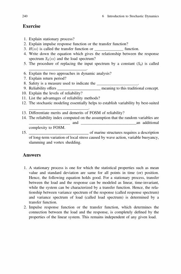
Exercise
1. Explain stationary process?2. Explain impulse response function or the transfer function?3. HðxÞ is called the transfer function or ______________ function.4. Write down the equation which gives the relationship between the response
spectrum SXðxÞ and the load spectrum?5. The procedure of replacing the input spectrum by a constant (S0) is called
____________________________.6. Explain the two approaches in dynamic analysis?7. Explain return period?8. Safety is a measure used to indicate the ____________________.9. Reliability offers _____________________ meaning to this traditional concept.
10. Explain the levels of reliability?11. List the advantages of reliability methods?12. The stochastic modeling essentially helps to establish variability by best-suited
_____________________________.13. Differentiate merits and demerits of FOSM of reliability?14. The reliability index computed on the assumption that the random variables are
____________________ and ___________________________an additionalcomplexity to FOSM.
15. _____________________________ of marine structures requires a descriptionof long-term variation of local stress caused by wave action, variable buoyancy,slamming and vortex shedding.
Answers
1. A stationary process is one for which the statistical properties such as meanvalue and standard deviation are same for all points in time (or) position.Hence, the following equation holds good. For a stationary process, transferbetween the load and the response can be modeled as linear, time-invariant,while the system can be characterized by a transfer function. Hence, the rela-tionship between variance spectrum of the response (called response spectrum)and variance spectrum of load (called load spectrum) is determined by atransfer function.
2. Impulse response function or the transfer function, which determines theconnection between the load and the response, is completely defined by theproperties of the linear system. This remains independent of any given load.
240 6 Introduction to Stochastic Dynamics
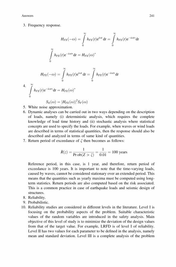
3. Frequency response.
HFXð�xÞ ¼Z10
hFXðtÞeixt dt ¼Z10
hFXðtÞe�ixt�dt
Z10
hFXðtÞe�ixt�dt ¼ HFXðxÞ�
4.
HFXð�xÞ ¼Z10
hFXðtÞeixt dt ¼Z10
hFXðtÞe�ixt�dt
Z10
hFXðtÞe�ixt�dt ¼ HFXðxÞ�
SXðxÞ ¼ HFXðxÞj j2SFðxÞ5. White noise approximation.6. Dynamic analyses can be carried out in two ways depending on the description
of loads, namely (i) deterministic analysis, which requires the completeknowledge of load time history and (ii) stochastic analysis where statisticalconcepts are used to specify the loads. For example, when waves or wind loadsare described in terms of statistical quantities, then the response should also bedescribed and analyzed in terms of same kind of quantities.
7. Return period of exceedance of ξ then becomes as follows:
�RðzÞ ¼ 1Pr obðZ[ nÞ ¼
10:01
¼ 100 years
Reference period, in this case, is 1 year, and therefore, return period ofexceedance is 100 years. It is important to note that the time-varying loads,caused by waves, cannot be considered stationary over an extended period. Thismeans that the quantities such as yearly maxima must be computed using long-term statistics. Return periods are also computed based on the risk associated.This is a common practice in case of earthquake loads and seismic design ofstructures.
8. Reliability.9. Probabilistic.
10. Reliability studies are considered in different levels in the literature. Level I isfocusing on the probability aspects of the problem. Suitable characteristicvalues of the random variables are introduced in the safety analysis. Mainobjective of this level of study is to minimize the deviation of the design valuesfrom that of the target value. For example, LRFD is of level I of reliability.Level II has two values for each parameter to be defined in the analysis, namelymean and standard deviation. Level III is a complete analysis of the problem
Answers 241

addressing the multi-dimensional probability density function of random vari-ables, which is extended over the safety domain. Reliability is expressed interms of suitable safety indices. In level IV, engineering economics is alsoapplied in the reliability study. This level of reliability study is usually appliedto structures of strategic importance. The study includes cost-benefit analysis,rehabilitation, consequence of failure, and return on capital investment.
11. The advantages of reliability methods are as listed below
• Offer a realistic procession of uncertainties and the methods for evaluatingthe safety factors that are often too arbitrary.
• Offer decision-making support for more economic and better balanceddesign.
• Analyze failure modes and measure the reliability provided by applicationand regulations.
• Allow the optimal distribution of material and arrange various componentsof the structure.
• Benefit from the experience acquired in design by updating on the basis offeedback from the experience.
• Expand the knowledge of uncertainty in response to the structure.
12. Probability density function.13.
14. Statistically independent and normally distributed poses.15. Fatigue design.
Advantages Disadvantages
It is easy to use Results can cause serious errors. The tool used for thedistribution function cannot be approximated bynormal distribution
It does not require knowledge ofdistribution of random variables
Values of β depend on the specific form of the limitstate function. This is an invariance problem
242 6 Introduction to Stochastic Dynamics
Chapter 7Applications in Preliminary Analysisand Design
Abstract This chapter deals with a few application problems in the design anddevelopment on new offshore structures based on the dynamic analyses. Studiespresented in this chapter are based on the recent research conducted by the author,which are presented as a part of intuitive studies to the readers.
Keywords Design � Offshore structures � Preliminary design � Triceratops �Buoyant leg structure � Ball joints � Response isolation � Structural forms � Wavedirectionality � Springing � Ringing � Tension leg platforms
7.1 Free Vibration Response of Offshore Triceratops
Offshore triceratops is relatively a new type of compliant structure suitable fordeepwater oil exploration. The structural form of the platform enables to counteractthe encountered environmental loads efficiently. Triceratops consists of three ormore buoyant leg structures (BLSs) to achieve the required buoyancy, to supportthe deck structure, to restrain system, and to serve storage requirements. The deckand BLSs are connected by ball joints that transfer translational motion but restrainrotations from BLS to deck and vice versa. Free-decay studies are conducted on1:150 scaled model, in free-floating and tethered conditions experimentally, ana-lytically and numerically; natural periods in heave and pitch/roll degrees of freedomare discussed for installation and decommissioning purposes. Experimental andanalytical free-decay tests are conducted on the installed structure in surge andheave degrees of freedom; experimental, analytical, and numerical results are ingood comparison. Based on the studies carried out, it is seen that the free-floatingnatural periods of both single BLS and tethered triceratops are away from thebandwidth of encountered wave periods, making the proposed platform safe andsuitable for the chosen sea state and ultra-deep waters.
© Springer India 2015S. Chandrasekaran, Dynamic Analysis and Design of Offshore Structures,Ocean Engineering & Oceanography 5, DOI 10.1007/978-81-322-2277-4_7
243
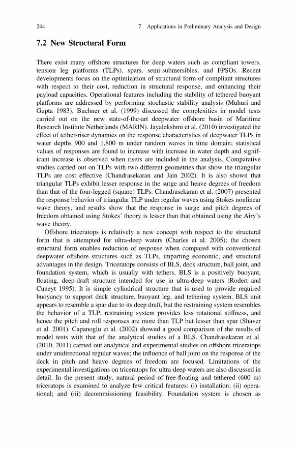
7.2 New Structural Form
There exist many offshore structures for deep waters such as compliant towers,tension leg platforms (TLPs), spars, semi-submersibles, and FPSOs. Recentdevelopments focus on the optimization of structural form of compliant structureswith respect to their cost, reduction in structural response, and enhancing theirpayload capacities. Operational features including the stability of tethered buoyantplatforms are addressed by performing stochastic stability analysis (Muhuri andGupta 1983). Buchner et al. (1999) discussed the complexities in model testscarried out on the new state-of-the-art deepwater offshore basin of MaritimeResearch Institute Netherlands (MARIN). Jayalekshmi et al. (2010) investigated theeffect of tether-riser dynamics on the response characteristics of deepwater TLPs inwater depths 900 and 1,800 m under random waves in time domain; statisticalvalues of responses are found to increase with increase in water depth and signif-icant increase is observed when risers are included in the analysis. Comparativestudies carried out on TLPs with two different geometries that show the triangularTLPs are cost effective (Chandrasekaran and Jain 2002). It is also shown thattriangular TLPs exhibit lesser response in the surge and heave degrees of freedomthan that of the four-legged (square) TLPs. Chandrasekaran et al. (2007) presentedthe response behavior of triangular TLP under regular waves using Stokes nonlinearwave theory, and results show that the response in surge and pitch degrees offreedom obtained using Stokes’ theory is lesser than that obtained using the Airy’swave theory.
Offshore triceratops is relatively a new concept with respect to the structuralform that is attempted for ultra-deep waters (Charles et al. 2005); the chosenstructural form enables reduction of response when compared with conventionaldeepwater offshore structures such as TLPs, imparting economic, and structuraladvantages in the design. Triceratops consists of BLS, deck structure, ball joint, andfoundation system, which is usually with tethers. BLS is a positively buoyant,floating, deep-draft structure intended for use in ultra-deep waters (Rodert andCuneyt 1995). It is simple cylindrical structure that is used to provide requiredbuoyancy to support deck structure, buoyant leg, and tethering system. BLS unitappears to resemble a spar due to its deep draft, but the restraining system resemblesthe behavior of a TLP; restraining system provides less rotational stiffness, andhence the pitch and roll responses are more than TLP but lesser than spar (Shaveret al. 2001). Capanoglu et al. (2002) showed a good comparison of the results ofmodel tests with that of the analytical studies of a BLS. Chandrasekaran et al.(2010, 2011) carried out analytical and experimental studies on offshore triceratopsunder unidirectional regular waves; the influence of ball joint on the response of thedeck in pitch and heave degrees of freedom are focused. Limitations of theexperimental investigations on triceratops for ultra-deep waters are also discussed indetail. In the present study, natural period of free-floating and tethered (600 m)triceratops is examined to analyze few critical features: (i) installation; (ii) opera-tional; and (iii) decommissioning feasibility. Foundation system is chosen as
244 7 Applications in Preliminary Analysis and Design
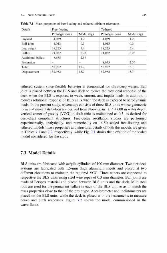
tethered system since flexible behavior is economical for ultra-deep waters. Balljoint is placed between the BLS and deck to reduce the rotational response of thedeck when the BLS is exposed to wave, current, and impact loads; in addition, itreduces rotational response of BLS units when the deck is exposed to aerodynamicloads. In the present study, triceratops consists of three BLS units whose geometricform and mass distribution are derived from Norwegian TLP at 600 m water depth;vertical center of gravity (VCG) to draft ratio is maintained as 0.5, as desired fordeep-draft compliant structures. Free-decay oscillation studies are performedexperimentally, analytically, and numerically on 1:150 scaled free-floating andtethered models; mass properties and structural details of both the models are givenin Tables 7.1 and 7.2, respectively, while Fig. 7.1 shows the elevation of the scaledmodel considered for the study.
7.3 Model Details
BLS units are fabricated with acrylic cylinders of 100 mm diameter. Two-tier decksystems are fabricated with 1.5-mm thick aluminum sheets and placed at twodifferent elevations to maintain the required VCG. Three tethers are connected torespective the BLS units using steel wire ropes of 0.3 mm diameter. Ball joints aremade of Perspex material and placed between BLS units and the deck. Mild steelrods are used for the permanent ballast in each of the BLS unit so as to match themass properties close to that of the prototype. Accelerometer and inclinometers areplaced on the BLS units, while the deck is placed with the instruments to measureheave and pitch responses. Figure 7.2 shows the model commissioned in thewave flume.
Table 7.1 Mass properties of free-floating and tethered offshore triceratops
Details Free-floating Tethered
Prototype (ton) Model (kg) Prototype (ton) Model (kg)
Payload 4,059 1.2 4,059 1.2
Ball joint 1,013 0.3 1,013 0.3
Leg weight 18,225 5.4 18,225 5.4
Ballast 21,032 6.23 21,032 6.23
Additional ballast 8,635 2.56 – –
Pretension – – 8,635 2.56
Total 52,982 15.7 52,982 15.7
Displacement 52,982 15.7 52,982 15.7
7.2 New Structural Form 245
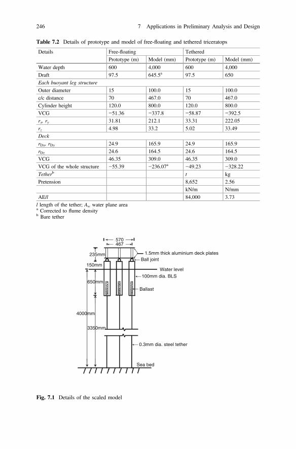
Table 7.2 Details of prototype and model of free-floating and tethered triceratops
Details Free-floating TetheredPrototype (m) Model (mm) Prototype (m) Model (mm)
Water depth 600 4,000 600 4,000Draft 97.5 645.5a 97.5 650Each buoyant leg structure
Outer diameter 15 100.0 15 100.0c/c distance 70 467.0 70 467.0Cylinder height 120.0 800.0 120.0 800.0VCG −51.36 −337.8 −58.87 −392.5rx, ry 31.81 212.1 33.31 222.05rz 4.98 33.2 5.02 33.49Deck
rDx, rDy 24.9 165.9 24.9 165.9rDz 24.6 164.5 24.6 164.5VCG 46.35 309.0 46.35 309.0VCG of the whole structure −55.39 −236.07a −49.23 −328.22Tetherb t kgPretension 8,652 2.56
kN/m N/mmAE/l 84,000 3.73l length of the tether; Aw water plane areaa Corrected to flume densityb Bare tether
570 467
235mm
150mm
650mm
3350mm
4000mm
Sea bed
0.3mm dia. steel tether
Ballast
100mm dia. BLSWater level
Ball joint1.5mm thick aluminium deck plates
Fig. 7.1 Details of the scaled model
246 7 Applications in Preliminary Analysis and Design
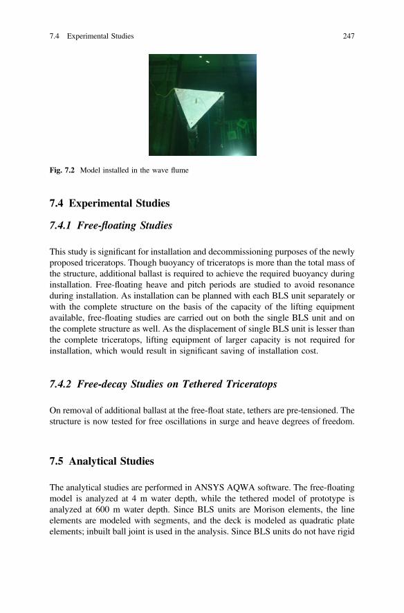
7.4 Experimental Studies
7.4.1 Free-floating Studies
This study is significant for installation and decommissioning purposes of the newlyproposed triceratops. Though buoyancy of triceratops is more than the total mass ofthe structure, additional ballast is required to achieve the required buoyancy duringinstallation. Free-floating heave and pitch periods are studied to avoid resonanceduring installation. As installation can be planned with each BLS unit separately orwith the complete structure on the basis of the capacity of the lifting equipmentavailable, free-floating studies are carried out on both the single BLS unit and onthe complete structure as well. As the displacement of single BLS unit is lesser thanthe complete triceratops, lifting equipment of larger capacity is not required forinstallation, which would result in significant saving of installation cost.
7.4.2 Free-decay Studies on Tethered Triceratops
On removal of additional ballast at the free-float state, tethers are pre-tensioned. Thestructure is now tested for free oscillations in surge and heave degrees of freedom.
7.5 Analytical Studies
The analytical studies are performed in ANSYS AQWA software. The free-floatingmodel is analyzed at 4 m water depth, while the tethered model of prototype isanalyzed at 600 m water depth. Since BLS units are Morison elements, the lineelements are modeled with segments, and the deck is modeled as quadratic plateelements; inbuilt ball joint is used in the analysis. Since BLS units do not have rigid
Fig. 7.2 Model installed in the wave flume
7.4 Experimental Studies 247
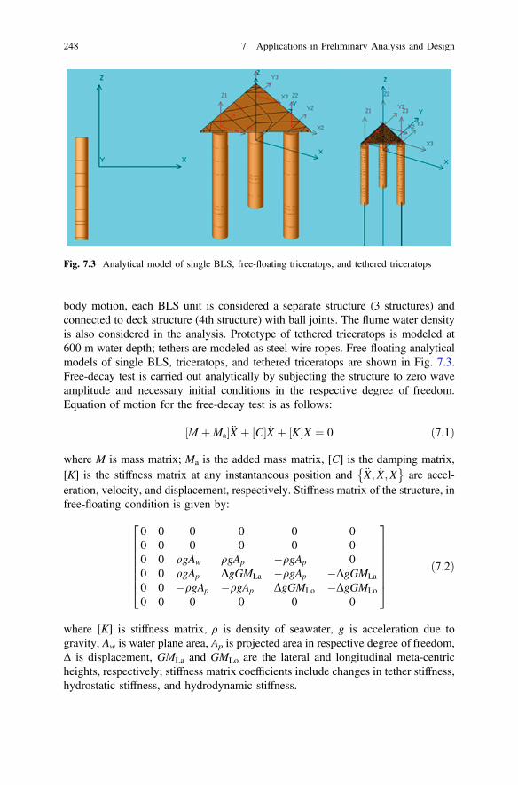
body motion, each BLS unit is considered a separate structure (3 structures) andconnected to deck structure (4th structure) with ball joints. The flume water densityis also considered in the analysis. Prototype of tethered triceratops is modeled at600 m water depth; tethers are modeled as steel wire ropes. Free-floating analyticalmodels of single BLS, triceratops, and tethered triceratops are shown in Fig. 7.3.Free-decay test is carried out analytically by subjecting the structure to zero waveamplitude and necessary initial conditions in the respective degree of freedom.Equation of motion for the free-decay test is as follows:
M þMa½ �€X þ C½ � _X þ ½K�X ¼ 0 ð7:1Þ
where M is mass matrix; Ma is the added mass matrix, [C] is the damping matrix,[K] is the stiffness matrix at any instantaneous position and €X; _X;X
� �are accel-
eration, velocity, and displacement, respectively. Stiffness matrix of the structure, infree-floating condition is given by:
0 0 0 0 0 00 0 0 0 0 00 0 qgAw qgAp �qgAp 00 0 qgAp DgGMLa �qgAp �DgGMLa
0 0 �qgAp �qgAp DgGMLo �DgGMLo
0 0 0 0 0 0
26666664
37777775
ð7:2Þ
where [K] is stiffness matrix, ρ is density of seawater, g is acceleration due togravity, Aw is water plane area, Ap is projected area in respective degree of freedom,Δ is displacement, GMLa and GMLo are the lateral and longitudinal meta-centricheights, respectively; stiffness matrix coefficients include changes in tether stiffness,hydrostatic stiffness, and hydrodynamic stiffness.
Fig. 7.3 Analytical model of single BLS, free-floating triceratops, and tethered triceratops
248 7 Applications in Preliminary Analysis and Design
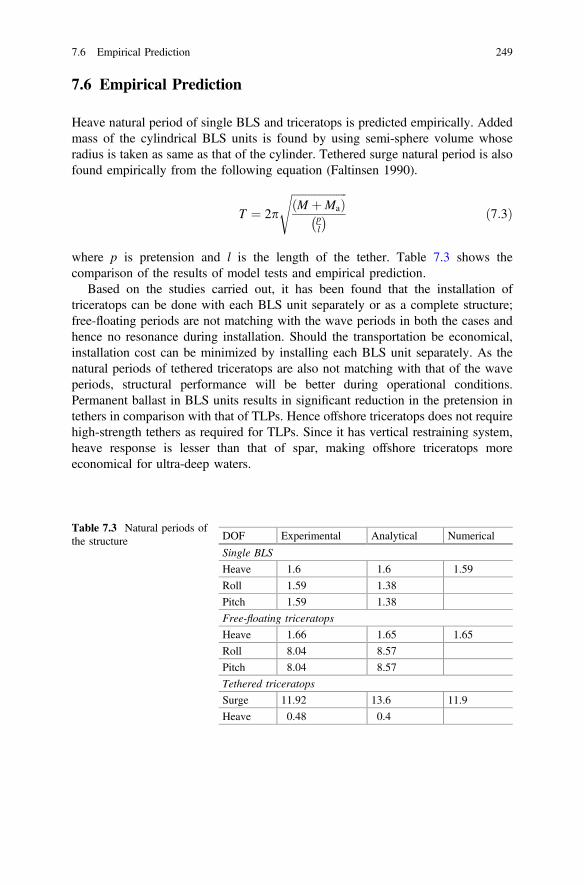
7.6 Empirical Prediction
Heave natural period of single BLS and triceratops is predicted empirically. Addedmass of the cylindrical BLS units is found by using semi-sphere volume whoseradius is taken as same as that of the cylinder. Tethered surge natural period is alsofound empirically from the following equation (Faltinsen 1990).
T ¼ 2p
ffiffiffiffiffiffiffiffiffiffiffiffiffiffiffiffiffiffiffiffiM þMað Þ
pl
� �s
ð7:3Þ
where p is pretension and l is the length of the tether. Table 7.3 shows thecomparison of the results of model tests and empirical prediction.
Based on the studies carried out, it has been found that the installation oftriceratops can be done with each BLS unit separately or as a complete structure;free-floating periods are not matching with the wave periods in both the cases andhence no resonance during installation. Should the transportation be economical,installation cost can be minimized by installing each BLS unit separately. As thenatural periods of tethered triceratops are also not matching with that of the waveperiods, structural performance will be better during operational conditions.Permanent ballast in BLS units results in significant reduction in the pretension intethers in comparison with that of TLPs. Hence offshore triceratops does not requirehigh-strength tethers as required for TLPs. Since it has vertical restraining system,heave response is lesser than that of spar, making offshore triceratops moreeconomical for ultra-deep waters.
Table 7.3 Natural periods ofthe structure DOF Experimental Analytical Numerical
Single BLS
Heave 1.6 1.6 1.59
Roll 1.59 1.38
Pitch 1.59 1.38
Free-floating triceratops
Heave 1.66 1.65 1.65
Roll 8.04 8.57
Pitch 8.04 8.57
Tethered triceratops
Surge 11.92 13.6 11.9
Heave 0.48 0.4
7.6 Empirical Prediction 249
7.7 Wave Directionality Effects on Offshore Triceratops
The primary objective of the current study is to investigate the nonlinear dynamicresponse characteristics of offshore triceratops under regular waves for differentwave approach angles. In the present study, 1:150 scaled model of offshore tri-ceratops is investigated under regular waves by varying the wave period. Geometriccharacteristics of the platform and mass distribution are derived from NorwegianTLP (Minoo and Joel 1991) at a water depth of 600 m for equivalent buoyancy asthat of the TLP. Buoyancy of pontoons of TLP is distributed to each BLS unit byincreasing its draft; this is required to ascertain symmetric response in all BLS unitsfor the considered wave approach angles. Mass distribution and geometric prop-erties are given in Tables 7.4 and 7.5, respectively. BLS units are fabricated withacrylic material, and PVC ball joints are placed between the deck and the BLSunits. Deck consists of two aluminum plates of 570 mm width and 1.5 mmthickness that are placed at two levels so as to obtain the representative value ofcenter of gravity of the deck. In order to ensure equal payload distribution on eachBLS unit, triangular geometry of the deck plate is chosen for the study; center ofgravity of the BLS units and the deck is maintained on the same vertical axis.Components of the triceratops are shown in Fig. 7.4. Figure 7.5 shows the 1:150scaled model considered for the study. The model is free-floated by ballasting eachBLS unit; ballast mass is kept equivalent to the amount of pretension in each tether.Experimental studies are carried out in the wave flume of 4 m width, at a waterdepth of 4 m. Details of prototype and scaled wave data are given in the Tables 7.4and 7.5. Dynamic response of the platform is measured for three different waveapproach angles with reference to the axis of symmetry of the structure; details ofinstrumentation are shown in Fig. 7.6. Two accelerometers (surge/sway of BLS,heave of deck) and two inclinometers (pitch/roll of BLS and deck) are used tomeasure the acceleration and pitch responses. Surge, heave, and pitch RAOs(response amplitude operators) of the model are scaled up to the prototype andplotted for BLS units and the deck under the regular wave loads; three waveapproach angles namely 0°, 90°, and 180° are considered in the present study.
7.8 Discussions of Experimental Studies
Free oscillation tests are conducted on free-floating and tethered models of thestructure to determine their natural periods of vibration. These tests are conductedin two stages: (i) each BLS is freely floated by ballasting, while free oscillation testsare conducted on single BLS in heave and pitch degrees of freedom; and (ii) deck isconnected to BLS units through ball joints for a desired draft of 650 mm, andsubsequently free oscillation tests are conducted on the whole platform. Tethers arethen connected to the model, and the platform is de-ballasted to enable the desiredpre-tension in tethers. Free-floating natural periods and theirs scaled-up values of
250 7 Applications in Preliminary Analysis and Design
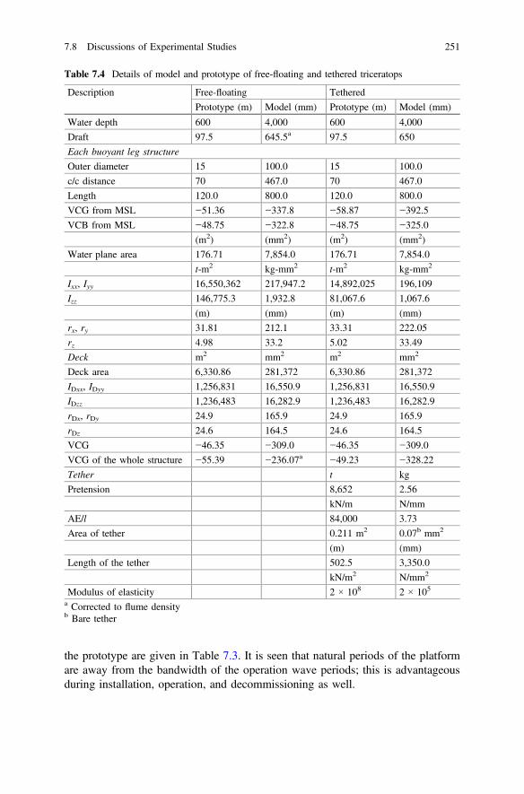
the prototype are given in Table 7.3. It is seen that natural periods of the platformare away from the bandwidth of the operation wave periods; this is advantageousduring installation, operation, and decommissioning as well.
Table 7.4 Details of model and prototype of free-floating and tethered triceratops
Description Free-floating Tethered
Prototype (m) Model (mm) Prototype (m) Model (mm)
Water depth 600 4,000 600 4,000
Draft 97.5 645.5a 97.5 650
Each buoyant leg structure
Outer diameter 15 100.0 15 100.0
c/c distance 70 467.0 70 467.0
Length 120.0 800.0 120.0 800.0
VCG from MSL −51.36 −337.8 −58.87 −392.5
VCB from MSL −48.75 −322.8 −48.75 −325.0
(m2) (mm2) (m2) (mm2)
Water plane area 176.71 7,854.0 176.71 7,854.0
t-m2 kg-mm2 t-m2 kg-mm2
Ixx, Iyy 16,550,362 217,947.2 14,892,025 196,109
Izz 146,775.3 1,932.8 81,067.6 1,067.6
(m) (mm) (m) (mm)
rx, ry 31.81 212.1 33.31 222.05
rz 4.98 33.2 5.02 33.49
Deck m2 mm2 m2 mm2
Deck area 6,330.86 281,372 6,330.86 281,372
IDxx, IDyy 1,256,831 16,550.9 1,256,831 16,550.9
IDzz 1,236,483 16,282.9 1,236,483 16,282.9
rDx, rDy 24.9 165.9 24.9 165.9
rDz 24.6 164.5 24.6 164.5
VCG −46.35 −309.0 −46.35 −309.0
VCG of the whole structure −55.39 −236.07a −49.23 −328.22
Tether t kg
Pretension 8,652 2.56
kN/m N/mm
AE/l 84,000 3.73
Area of tether 0.211 m2 0.07b mm2
(m) (mm)
Length of the tether 502.5 3,350.0
kN/m2 N/mm2
Modulus of elasticity 2 × 10⁸ 2 × 10⁵
a Corrected to flume densityb Bare tether
7.8 Discussions of Experimental Studies 251
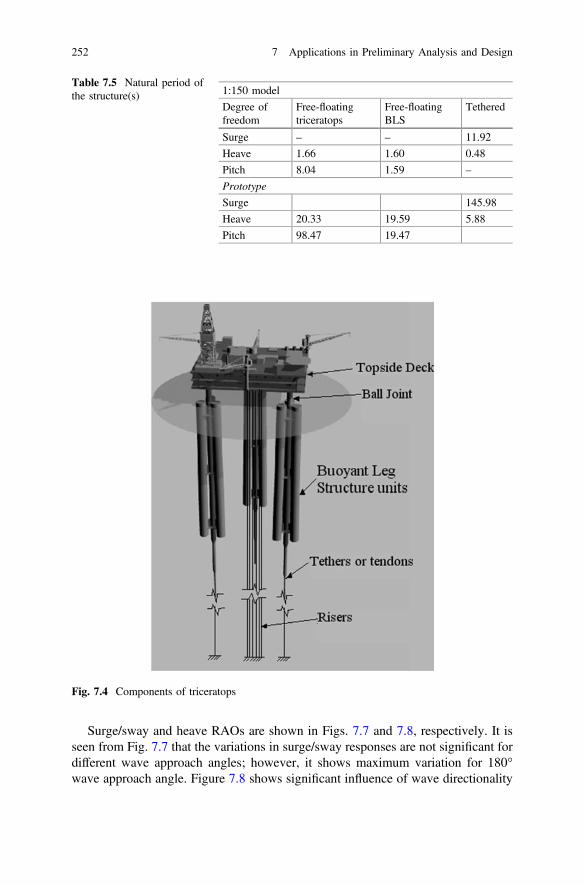
Surge/sway and heave RAOs are shown in Figs. 7.7 and 7.8, respectively. It isseen from Fig. 7.7 that the variations in surge/sway responses are not significant fordifferent wave approach angles; however, it shows maximum variation for 180°wave approach angle. Figure 7.8 shows significant influence of wave directionality
Table 7.5 Natural period ofthe structure(s) 1:150 model
Degree offreedom
Free-floatingtriceratops
Free-floatingBLS
Tethered
Surge – – 11.92
Heave 1.66 1.60 0.48
Pitch 8.04 1.59 –
Prototype
Surge 145.98
Heave 20.33 19.59 5.88
Pitch 98.47 19.47
Fig. 7.4 Components of triceratops
252 7 Applications in Preliminary Analysis and Design
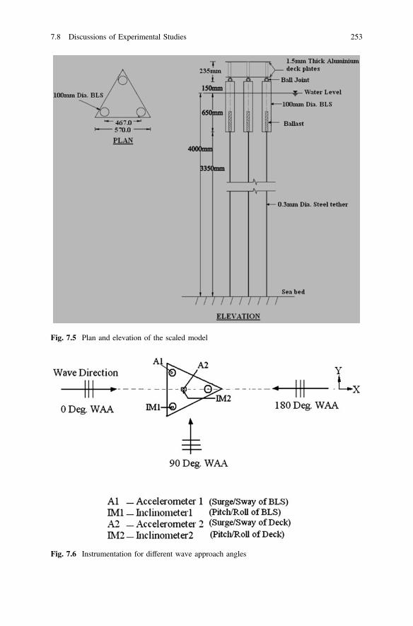
Fig. 7.5 Plan and elevation of the scaled model
Fig. 7.6 Instrumentation for different wave approach angles
7.8 Discussions of Experimental Studies 253
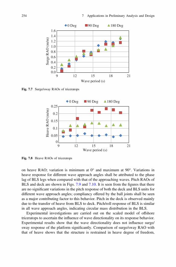
on heave RAO; variation is minimum at 0° and maximum at 90°. Variations inheave response for different wave approach angles shall be attributed to the phaselag of BLS legs when compared with that of the approaching waves. Pitch RAOs ofBLS and deck are shown in Figs. 7.9 and 7.10. It is seen from the figures that thereare no significant variations in the pitch response of both the deck and BLS units fordifferent wave approach angles; compliancy offered by the ball joints shall be seenas a major contributing factor to this behavior. Pitch in the deck is observed mainlydue to the transfer of heave from BLS to deck. Pitch/roll response of BLS is similarin all wave approach angles, indicating circular mass distribution in the BLS.
Experimental investigations are carried out on the scaled model of offshoretriceratops to ascertain the influence of wave directionality on its response behavior.Experimental results show that the wave directionality does not influence surge/sway response of the platform significantly. Comparison of surge/sway RAO withthat of heave shows that the structure is restrained in heave degree of freedom,
0.00.2
0.4
0.6
0.8
1.0
1.2
1.4
1.6
9 12 15 18 21
Surg
e R
AO
(m
/m)
Wave period (s)
0 Deg 90 Deg 180 Deg
Fig. 7.7 Surge/sway RAOs of triceratops
0
0.05
0.1
0.15
0.2
0.25
9 12 15 18 21
Hea
ve R
AO
(m
/m)
Wave period (s)
0 Deg 90 Deg 180 Deg
Fig. 7.8 Heave RAOs of triceratops
254 7 Applications in Preliminary Analysis and Design
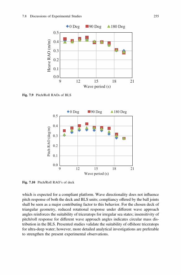
which is expected for a compliant platform. Wave directionality does not influencepitch response of both the deck and BLS units; compliancy offered by the ball jointsshall be seen as a major contributing factor to this behavior. For the chosen deck oftriangular geometry, reduced rotational response under different wave approachangles reinforces the suitability of triceratops for irregular sea states; insensitivity ofpitch/roll response for different wave approach angles indicates circular mass dis-tribution in the BLS. Presented studies validate the suitability of offshore triceratopsfor ultra-deep water; however, more detailed analytical investigations are preferableto strengthen the present experimental observations.
0.0
0.1
0.2
0.3
0.4
0.5
9 12 15 18 21
Hea
ve R
AO
(m
/m)
Wave period (s)
0 Deg 90 Deg 180 Deg
Fig. 7.9 Pitch/Roll RAOs of BLS
0.0
0.1
0.2
0.3
0.4
0.5
9 12 15 18 21
Pitc
h R
AO
(deg
/m)
Wave period (s)
0 Deg 90 Deg 180 Deg
Fig. 7.10 Pitch/Roll RAO’s of deck
7.8 Discussions of Experimental Studies 255
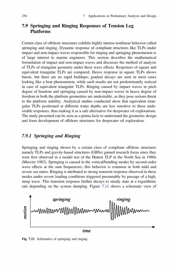
7.9 Springing and Ringing Responses of Tension LegPlatforms
Certain class of offshore structures exhibits highly intense nonlinear behavior calledspringing and ringing. Dynamic response of compliant structures like TLPs underimpact and non-impact waves responsible for ringing and springing phenomenon isof large interest to marine engineers. This section describes the mathematicalformulation of impact and non-impact waves and discusses the method of analysisof TLPs of triangular geometry under these wave effects. Responses of square andequivalent triangular TLPs are compared. Heave response in square TLPs showsbursts, but there are no rapid buildups; gradual decays are seen in most caseslooking like a beat phenomenon, while such results are not predominantly noticedin case of equivalent triangular TLPs. Ringing caused by impact waves in pitchdegree of freedom and springing caused by non-impact waves in heave degree offreedom in both the platform geometries are undesirable, as they pose serious threatto the platform stability. Analytical studies conducted show that equivalent trian-gular TLPs positioned at different water depths are less sensitive to these unde-sirable responses, thus making it as a safe alternative for deepwater oil explorations.The study presented can be seen as a prima facie to understand the geometric designand form development of offshore structures for deepwater oil exploration.
7.9.1 Springing and Ringing
Springing and ringing shown by a certain class of compliant offshore structuresnamely TLPs and gravity-based structures (GBSs) gained research focus since theywere first observed in a model test of the Hutton TLP in the North Sea in 1980s(Mercier 1982). Springing is caused in the vertical/bending modes by second-orderwave effects at the sum frequencies; this behavior is common in both mild andsevere sea states. Ringing is attributed to strong transient response observed in thesemodes under severe loading conditions triggered presumably by passage of a high,steep wave. This transient response further decays to steady state at a logarithmicrate depending on the system damping. Figure 7.11 shows a schematic view of
Fig. 7.11 Schematics of springing and ringing
256 7 Applications in Preliminary Analysis and Design
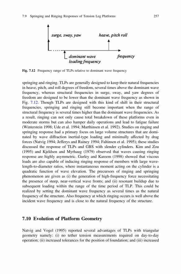
springing and ringing. TLPs are generally designed to keep their natural frequenciesin heave, pitch, and roll degrees of freedom, several times above the dominant wavefrequency, whereas structural frequencies in surge, sway, and yaw degrees offreedom are designed to be lower than the dominant wave frequency as shown inFig. 7.12. Though TLPs are designed with this kind of shift in their structuralfrequencies, springing and ringing still become important when the range ofstructural frequency is several times higher than the dominant wave frequencies. Asa result, ringing can not only cause total breakdown of these platforms even inmoderate storms but can also hamper daily operations and lead to fatigue failure(Winterstein 1998; Ude et al. 1994; Marthinsen et al. 1992). Studies on ringing andspringing response had a primary focus on large volume structures that are domi-nated by wave diffraction inertial-type loading and minimally affected by dragforces (Natvig 1994; Jefferys and Rainey 1994; Faltinsen et al. 1995); these studiesdiscussed the response of TLPs and GBS with slender cylinders. Kim and Zou(1995) and Kjeldsen and Myrhaug (1979) observed that waves causing ringingresponse are highly asymmetric. Gurley and Kareem (1998) showed that viscousloads are also capable of inducing ringing response of members with large wave-length-to-diameter ratios, where instantaneous moment acting on the cylinder is aquadratic function of wave elevation. The precursors of ringing and springingphenomenon are given as (i) the generation of high-frequency force necessitatingthe presence of steep, near-vertical wave fronts; and (ii) resonant buildup due tosubsequent loading within the range of the time period of TLP. This could berealized by setting the dominant wave frequency as several times as the naturalfrequency of the structure. Also frequency at which ringing occurs is well above theincident wave frequency and is close to the natural frequency of the structure.
7.10 Evolution of Platform Geometry
Natvig and Vogel (1995) reported several advantages of TLPs with triangulargeometry namely: (i) no tether tension measurements required on day-to-dayoperation; (ii) increased tolerances for the position of foundation; and (iii) increased
Fig. 7.12 Frequency range of TLPs relative to dominant wave frequency
7.9 Springing and Ringing Responses of Tension Leg Platforms 257
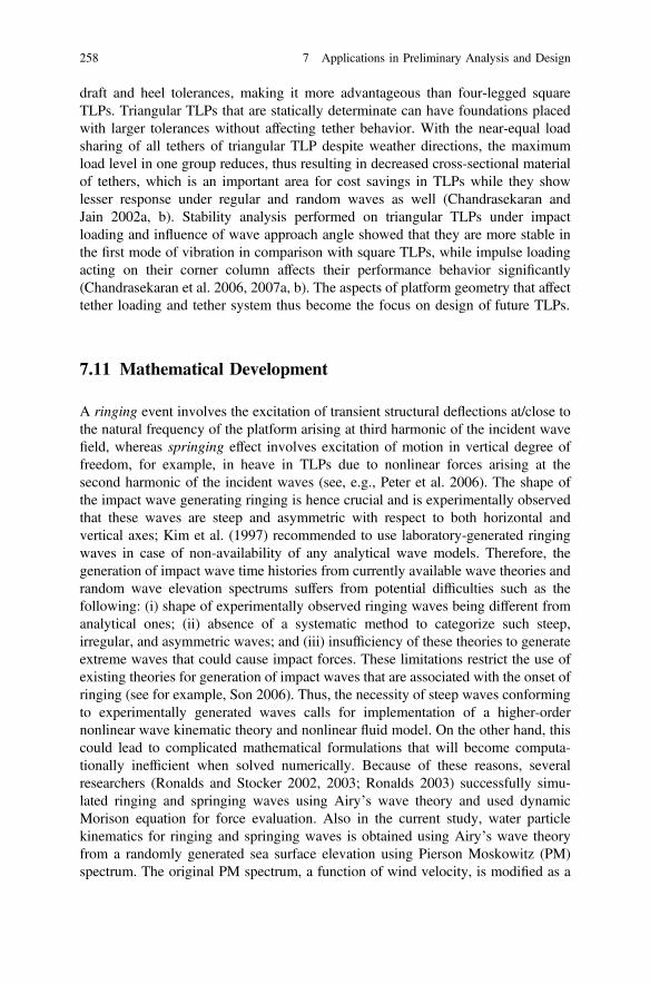
draft and heel tolerances, making it more advantageous than four-legged squareTLPs. Triangular TLPs that are statically determinate can have foundations placedwith larger tolerances without affecting tether behavior. With the near-equal loadsharing of all tethers of triangular TLP despite weather directions, the maximumload level in one group reduces, thus resulting in decreased cross-sectional materialof tethers, which is an important area for cost savings in TLPs while they showlesser response under regular and random waves as well (Chandrasekaran andJain 2002a, b). Stability analysis performed on triangular TLPs under impactloading and influence of wave approach angle showed that they are more stable inthe first mode of vibration in comparison with square TLPs, while impulse loadingacting on their corner column affects their performance behavior significantly(Chandrasekaran et al. 2006, 2007a, b). The aspects of platform geometry that affecttether loading and tether system thus become the focus on design of future TLPs.
7.11 Mathematical Development
A ringing event involves the excitation of transient structural deflections at/close tothe natural frequency of the platform arising at third harmonic of the incident wavefield, whereas springing effect involves excitation of motion in vertical degree offreedom, for example, in heave in TLPs due to nonlinear forces arising at thesecond harmonic of the incident waves (see, e.g., Peter et al. 2006). The shape ofthe impact wave generating ringing is hence crucial and is experimentally observedthat these waves are steep and asymmetric with respect to both horizontal andvertical axes; Kim et al. (1997) recommended to use laboratory-generated ringingwaves in case of non-availability of any analytical wave models. Therefore, thegeneration of impact wave time histories from currently available wave theories andrandom wave elevation spectrums suffers from potential difficulties such as thefollowing: (i) shape of experimentally observed ringing waves being different fromanalytical ones; (ii) absence of a systematic method to categorize such steep,irregular, and asymmetric waves; and (iii) insufficiency of these theories to generateextreme waves that could cause impact forces. These limitations restrict the use ofexisting theories for generation of impact waves that are associated with the onset ofringing (see for example, Son 2006). Thus, the necessity of steep waves conformingto experimentally generated waves calls for implementation of a higher-ordernonlinear wave kinematic theory and nonlinear fluid model. On the other hand, thiscould lead to complicated mathematical formulations that will become computa-tionally inefficient when solved numerically. Because of these reasons, severalresearchers (Ronalds and Stocker 2002, 2003; Ronalds 2003) successfully simu-lated ringing and springing waves using Airy’s wave theory and used dynamicMorison equation for force evaluation. Also in the current study, water particlekinematics for ringing and springing waves is obtained using Airy’s wave theoryfrom a randomly generated sea surface elevation using Pierson Moskowitz (PM)spectrum. The original PM spectrum, a function of wind velocity, is modified as a
258 7 Applications in Preliminary Analysis and Design
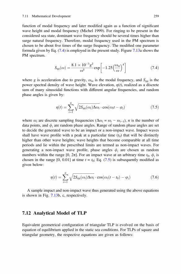
function of modal frequency and later modified again as a function of significantwave height and modal frequency (Michel 1999). For ringing to be present in theconsidered sea state, dominant wave frequency should be several times higher thansurge natural frequency. Therefore, modal frequency used in the PM spectrum ischosen to be about five times of the surge frequency. The modified one parameterformula given by Eq. (7.4) is employed in the present study. Figure 7.13a shows thePM spectrum.
Sgg xð Þ ¼ 8:1� 10�3g2
x5 exp �1:25xm
x
� �4
ð7:4Þ
where g is acceleration due to gravity, ωm is the modal frequency, and Sηη is thepower spectral density of wave height. Wave elevation, η(t), realized as a discretesum of many sinusoidal functions with different angular frequencies, and randomphase angles is given by:
g tð Þ ¼Xni¼1
ffiffiffiffiffiffiffiffiffiffiffiffiffiffiffiffiffiffiffiffiffiffiffiffiffi2Sgg xið ÞDxi
q� cos xit � uið Þ ð7:5Þ
where ωi are discrete sampling frequencies (Dωi = ωi − ωi−1), n is the number ofdata points, and /i are random phase angles. Range of random phase angles are setto decide the generated wave to be an impact or a non-impact wave. Impact wavesshall have wave profile with a peak at a particular time (t0) that will be distinctlyhigher than other wave heights; wave heights that become comparable at all timeperiods and lie within the prescribed limits are termed as non-impact waves. Forgenerating a non-impact wave profile, phase angles /i are chosen as randomnumbers within the range [0, 2π]. For an impact wave at an arbitrary time t0, /i ischosen in the range [0, 0.01] at time t = t0; Eq. (7.5) is subsequently modified asgiven below:
g tð Þ ¼Xni¼1
ffiffiffiffiffiffiffiffiffiffiffiffiffiffiffiffiffiffiffiffiffiffiffiffiffi2Sgg xið ÞDxi
q� cos xi t � t0ð Þ � uið Þ ð7:6Þ
A sample impact and non-impact wave thus generated using the above equationsis shown in Fig. 7.13b, c, respectively.
7.12 Analytical Model of TLP
Equivalent geometrical configuration of triangular TLP is evolved on the basis ofequation of equilibrium applied in the static sea conditions. For TLPs of square andtriangular geometry, the respective equations are given as follows:
7.11 Mathematical Development 259
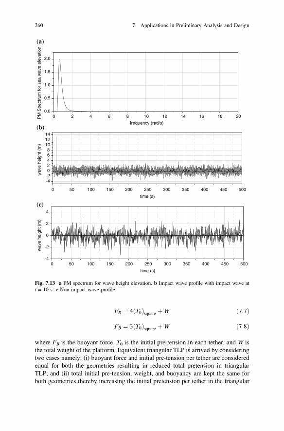
FB ¼ 4ðT0Þsquare þW ð7:7Þ
FB ¼ 3ðT0Þsquare þW ð7:8Þ
where FB is the buoyant force, T0 is the initial pre-tension in each tether, and W isthe total weight of the platform. Equivalent triangular TLP is arrived by consideringtwo cases namely: (i) buoyant force and initial pre-tension per tether are consideredequal for both the geometries resulting in reduced total pretension in triangularTLP; and (ii) total initial pre-tension, weight, and buoyancy are kept the same forboth geometries thereby increasing the initial pretension per tether in the triangular
0 2 4 6 8 10 12 14 16 18 200.0
0.5
1.0
1.5
2.0
(a)
(b)
(c)
PM
Spe
ctru
m fo
r se
a w
ave
elev
atio
n
frequency (rad/s)
0 50 100 150 200 250 300 350 400 450 500
-4-202468
101214
wav
e he
ight
(m
)
time (s)
0 50 100 150 200 250 300 350 400 450 500-4
-2
0
2
4
wav
e he
ight
(m
)
time (s)
Fig. 7.13 a PM spectrum for wave height elevation. b Impact wave profile with impact wave att = 10 s. c Non-impact wave profile
260 7 Applications in Preliminary Analysis and Design
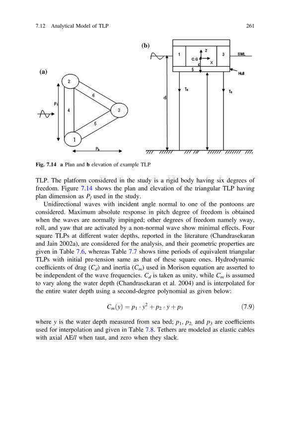
TLP. The platform considered in the study is a rigid body having six degrees offreedom. Figure 7.14 shows the plan and elevation of the triangular TLP havingplan dimension as Pl used in the study.
Unidirectional waves with incident angle normal to one of the pontoons areconsidered. Maximum absolute response in pitch degree of freedom is obtainedwhen the waves are normally impinged; other degrees of freedom namely sway,roll, and yaw that are activated by a non-normal wave show minimal effects. Foursquare TLPs at different water depths, reported in the literature (Chandrasekaranand Jain 2002a), are considered for the analysis, and their geometric properties aregiven in Table 7.6, whereas Table 7.7 shows time periods of equivalent triangularTLPs with initial pre-tension same as that of these square ones. Hydrodynamiccoefficients of drag (Cd) and inertia (Cm) used in Morison equation are asserted tobe independent of the wave frequencies. Cd is taken as unity, while Cm is assumedto vary along the water depth (Chandrasekaran et al. 2004) and is interpolated forthe entire water depth using a second-degree polynomial as given below:
Cm yð Þ ¼ p1 � y2 þ p2 � yþ p3 ð7:9Þ
where y is the water depth measured from sea bed; p1, p2, and p3 are coefficientsused for interpolation and given in Table 7.8. Tethers are modeled as elastic cableswith axial AE/l when taut, and zero when they slack.
Fig. 7.14 a Plan and b elevation of example TLP
7.12 Analytical Model of TLP 261
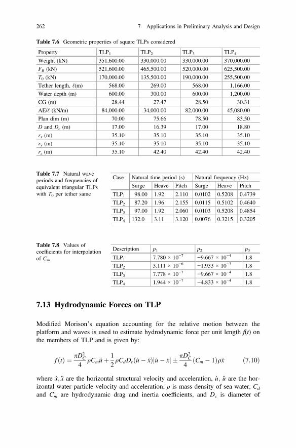
7.13 Hydrodynamic Forces on TLP
Modified Morison’s equation accounting for the relative motion between theplatform and waves is used to estimate hydrodynamic force per unit length f(t) onthe members of TLP and is given by:
f ðtÞ ¼ pD2C
4qCm€uþ 1
2qCdDcð _u� _xÞ _u� _xj j � pD2
C
4ðCm � 1Þq€x ð7:10Þ
where _x;€x are the horizontal structural velocity and acceleration, _u; €u are the hor-izontal water particle velocity and acceleration, ρ is mass density of sea water, Cd
and Cm are hydrodynamic drag and inertia coefficients, and Dc is diameter of
Table 7.6 Geometric properties of square TLPs considered
Property TLP1 TLP2 TLP3 TLP4Weight (kN) 351,600.00 330,000.00 330,000.00 370,000.00
FB (kN) 521,600.00 465,500.00 520,000.00 625,500.00
T0 (kN) 170,000.00 135,500.00 190,000.00 255,500.00
Tether length, ‘(m) 568.00 269.00 568.00 1,166.00
Water depth (m) 600.00 300.00 600.00 1,200.00
CG (m) 28.44 27.47 28.50 30.31
AE/‘ (kN/m) 84,000.00 34,000.00 82,000.00 45,080.00
Plan dim (m) 70.00 75.66 78.50 83.50
D and Dc (m) 17.00 16.39 17.00 18.80
rx (m) 35.10 35.10 35.10 35.10
ry (m) 35.10 35.10 35.10 35.10
rz (m) 35.10 42.40 42.40 42.40
Table 7.7 Natural waveperiods and frequencies ofequivalent triangular TLPswith T0 per tether same
Case Natural time period (s) Natural frequency (Hz)
Surge Heave Pitch Surge Heave Pitch
TLP1 98.00 1.92 2.110 0.0102 0.5208 0.4739
TLP2 87.20 1.96 2.155 0.0115 0.5102 0.4640
TLP3 97.00 1.92 2.060 0.0103 0.5208 0.4854
TLP4 132.0 3.11 3.120 0.0076 0.3215 0.3205
Table 7.8 Values ofcoefficients for interpolationof Cm
Description p1 p2 p3TLP1 7.780 × 10⁻⁷ −9.667 × 10⁻⁴ 1.8
TLP2 3.111 × 10⁻⁶ −1.933 × 10⁻³ 1.8
TLP3 7.778 × 10⁻⁷ −9.667 × 10⁻⁴ 1.8
TLP4 1.944 × 10⁻⁷ −4.833 × 10⁻⁴ 1.8
262 7 Applications in Preliminary Analysis and Design
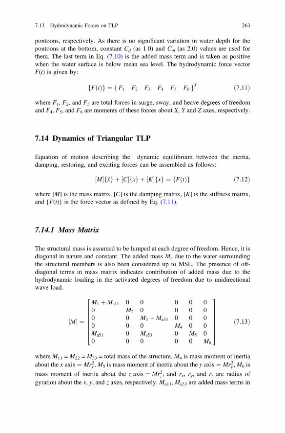
pontoons, respectively. As there is no significant variation in water depth for thepontoons at the bottom, constant Cd (as 1.0) and Cm (as 2.0) values are used forthem. The last term in Eq. (7.10) is the added mass term and is taken as positivewhen the water surface is below mean sea level. The hydrodynamic force vectorF(t) is given by:
FðtÞf g ¼ F1 F2 F3 F4 F5 F6f gT ð7:11Þ
where F1, F2, and F3 are total forces in surge, sway, and heave degrees of freedomand F4, F5, and F6 are moments of these forces about X, Y and Z axes, respectively.
7.14 Dynamics of Triangular TLP
Equation of motion describing the dynamic equilibrium between the inertia,damping, restoring, and exciting forces can be assembled as follows:
½M�f€xg þ ½C�f _xg þ ½K�fxg ¼ fFðtÞg ð7:12Þ
where [M] is the mass matrix, [C] is the damping matrix, [K] is the stiffness matrix,and {F(t)} is the force vector as defined by Eq. (7.11).
7.14.1 Mass Matrix
The structural mass is assumed to be lumped at each degree of freedom. Hence, it isdiagonal in nature and constant. The added mass Ma due to the water surroundingthe structural members is also been considered up to MSL. The presence of off-diagonal terms in mass matrix indicates contribution of added mass due to thehydrodynamic loading in the activated degrees of freedom due to unidirectionalwave load.
½M� ¼
M1 þMa11 0 0 0 0 00 M2 0 0 0 00 0 M3 þMa33 0 0 00 0 0 M4 0 0Ma51 0 Ma53 0 M5 00 0 0 0 0 M6
26666664
37777775
ð7:13Þ
where M11 = M22 = M33 = total mass of the structure, M4 is mass moment of inertiaabout the x axis ¼ Mr2x ,M5 is mass moment of inertia about the y axis ¼ Mr2y ,M6 is
mass moment of inertia about the z axis ¼ Mr2z , and rx, ry, and rz are radius ofgyration about the x, y, and z axes, respectively. Ma11, Ma33 are added mass terms in
7.13 Hydrodynamic Forces on TLP 263
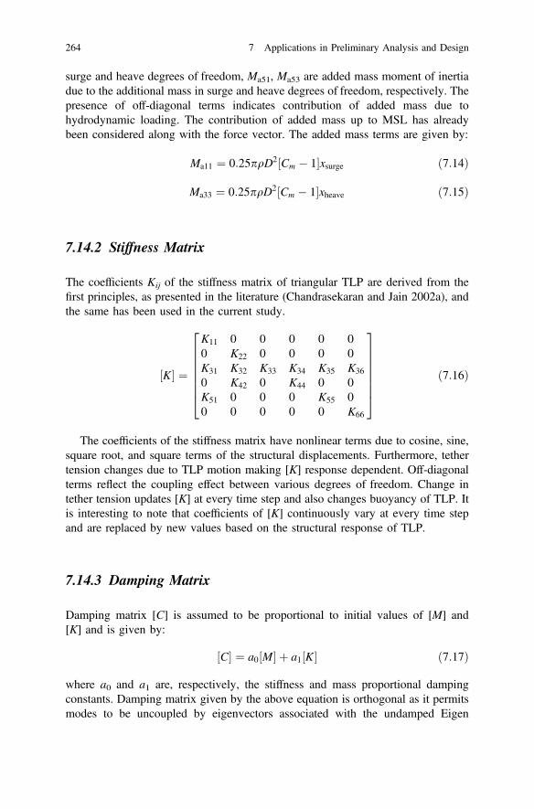
surge and heave degrees of freedom, Ma51, Ma53 are added mass moment of inertiadue to the additional mass in surge and heave degrees of freedom, respectively. Thepresence of off-diagonal terms indicates contribution of added mass due tohydrodynamic loading. The contribution of added mass up to MSL has alreadybeen considered along with the force vector. The added mass terms are given by:
Ma11 ¼ 0:25pqD2 Cm � 1½ �xsurge ð7:14Þ
Ma33 ¼ 0:25pqD2 Cm � 1½ �xheave ð7:15Þ
7.14.2 Stiffness Matrix
The coefficients Kij of the stiffness matrix of triangular TLP are derived from thefirst principles, as presented in the literature (Chandrasekaran and Jain 2002a), andthe same has been used in the current study.
½K� ¼
K11 0 0 0 0 00 K22 0 0 0 0K31 K32 K33 K34 K35 K36
0 K42 0 K44 0 0K51 0 0 0 K55 00 0 0 0 0 K66
26666664
37777775
ð7:16Þ
The coefficients of the stiffness matrix have nonlinear terms due to cosine, sine,square root, and square terms of the structural displacements. Furthermore, tethertension changes due to TLP motion making [K] response dependent. Off-diagonalterms reflect the coupling effect between various degrees of freedom. Change intether tension updates [K] at every time step and also changes buoyancy of TLP. Itis interesting to note that coefficients of [K] continuously vary at every time stepand are replaced by new values based on the structural response of TLP.
7.14.3 Damping Matrix
Damping matrix [C] is assumed to be proportional to initial values of [M] and[K] and is given by:
½C� ¼ a0 M½ � þ a1 K½ � ð7:17Þ
where a0 and a1 are, respectively, the stiffness and mass proportional dampingconstants. Damping matrix given by the above equation is orthogonal as it permitsmodes to be uncoupled by eigenvectors associated with the undamped Eigen
264 7 Applications in Preliminary Analysis and Design
problem. Damping constants a0 and a1 are determined by choosing the fractions ofcritical damping (ξ1 and ξ2) at two different frequencies (ω1 and ω2) and solvingsimultaneous equations for a0 and a1.
a0 ¼ 2 n2x2 � n1x1ð Þ= x22 � x2
1
� � ð7:18Þ
a1 ¼ 2x1x2 n1x2 � n2x1ð Þ= x22 � x2
1
� � ð7:19Þ
Damping attributable to a0[K] increases with increasing frequency, whereasdamping attributable to a1[M] increases with decreasing frequency. In the currentstudy, value of these coefficients are obtained using the above equations by takingdamping ratio ζ = 0.05 in surge and yaw degrees of freedom. Free vibration analysisis performed to find out natural frequencies of the platform corresponding to thesedegrees of freedom and found that damping ratios maintain reasonable values for allthe other modes which are contributing significantly to the response. Initial pre-tension in all tethers is assumed to be equal and total pretension changes with themotion of platform. The equation of motion is solved in time domain by employingNewmark’s integration scheme by taking α = 0.25 and β = 0.5. The solutionprocedure incorporates the changes namely: (i) stiffness coefficients varyingwith tether tension; (ii) added mass varying with sea surface fluctuations; and(iii) evaluation of wave forces at instantaneous position of the displaced platformconsidering the fluid structure interaction. Behavior under wave loading becomesnonlinear, and components of the equation of motion at each step components areupdated. Ten terms in the power series are found to be sufficient to give conver-gence in the iterative scheme. The time step Δt has been taken as 0.1 s, which is arelatively small value in comparison with the natural period (Tn) and hence yieldsaccurate values for the response.
7.15 Ringing Response
Ringing is usually a phenomenon attributed to response of compliant structuressuch as TLPs under impact waves. Figures 7.15, 7.16 and 7.17 show heave, pitch,and surge responses of all four cases of TLPs under impact waves, namely(i) square TLPs; (ii) equivalent triangular TLPs with T0 per tether same as that ofsquare; and (iii) equivalent triangular TLPs with total T0 same as that square,respectively. It can be seen that the response is primarily triggered in pitch degree offreedom for a wide range of time period similar to the response of a bell vibratingfor a longer time when struck by a large impact force. This is noticed in both thegeometries of TLPs, which shall be attributed to a ringing response. Though asimilar response is noticed under the influence of non-impact waves also, it can beseen that the intensity of pitch response caused by the latter is less compared withthat caused by impact waves. By comparing the ringing response in pitch degree of
7.14 Dynamics of Triangular TLP 265
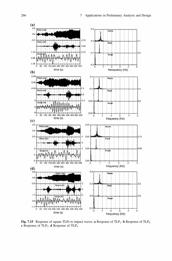
Fig. 7.15 Response of square TLPs to impact waves. a Response of TLP1. b Response of TLP2.c Response of TLP3. d Response of TLP4
266 7 Applications in Preliminary Analysis and Design
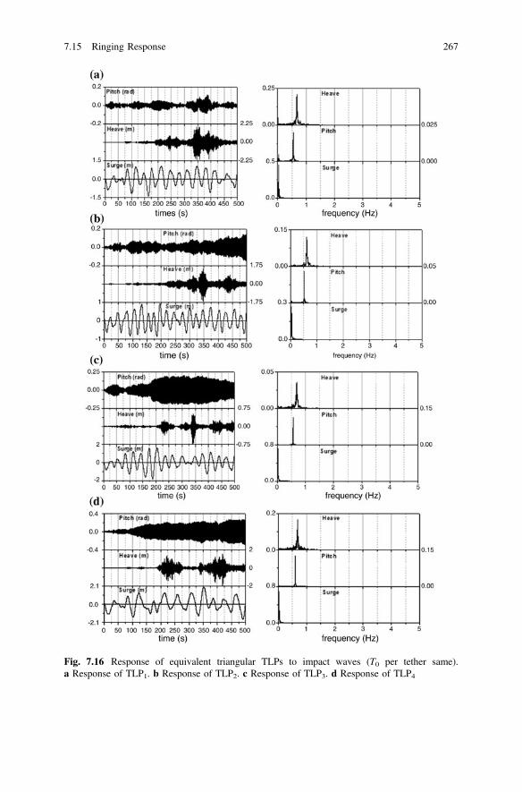
Fig. 7.16 Response of equivalent triangular TLPs to impact waves (T0 per tether same).a Response of TLP1. b Response of TLP2. c Response of TLP3. d Response of TLP4
7.15 Ringing Response 267
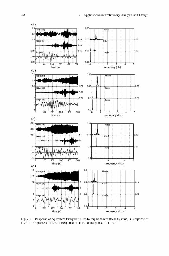
Fig. 7.17 Response of equivalent triangular TLPs to impact waves (total T0 same). a Response ofTLP1. b Response of TLP2. c Response of TLP3. d Response of TLP4
268 7 Applications in Preliminary Analysis and Design
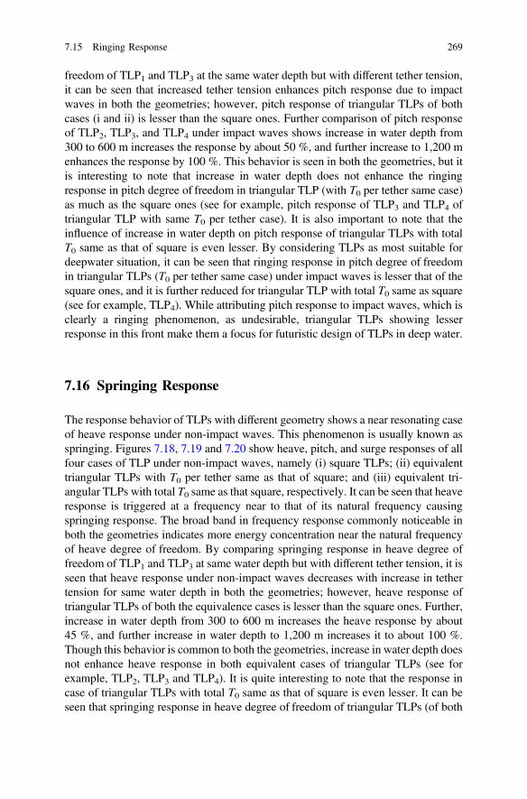
freedom of TLP1 and TLP3 at the same water depth but with different tether tension,it can be seen that increased tether tension enhances pitch response due to impactwaves in both the geometries; however, pitch response of triangular TLPs of bothcases (i and ii) is lesser than the square ones. Further comparison of pitch responseof TLP2, TLP3, and TLP4 under impact waves shows increase in water depth from300 to 600 m increases the response by about 50 %, and further increase to 1,200 menhances the response by 100 %. This behavior is seen in both the geometries, but itis interesting to note that increase in water depth does not enhance the ringingresponse in pitch degree of freedom in triangular TLP (with T0 per tether same case)as much as the square ones (see for example, pitch response of TLP3 and TLP4 oftriangular TLP with same T0 per tether case). It is also important to note that theinfluence of increase in water depth on pitch response of triangular TLPs with totalT0 same as that of square is even lesser. By considering TLPs as most suitable fordeepwater situation, it can be seen that ringing response in pitch degree of freedomin triangular TLPs (T0 per tether same case) under impact waves is lesser that of thesquare ones, and it is further reduced for triangular TLP with total T0 same as square(see for example, TLP4). While attributing pitch response to impact waves, which isclearly a ringing phenomenon, as undesirable, triangular TLPs showing lesserresponse in this front make them a focus for futuristic design of TLPs in deep water.
7.16 Springing Response
The response behavior of TLPs with different geometry shows a near resonating caseof heave response under non-impact waves. This phenomenon is usually known asspringing. Figures 7.18, 7.19 and 7.20 show heave, pitch, and surge responses of allfour cases of TLP under non-impact waves, namely (i) square TLPs; (ii) equivalenttriangular TLPs with T0 per tether same as that of square; and (iii) equivalent tri-angular TLPs with total T0 same as that square, respectively. It can be seen that heaveresponse is triggered at a frequency near to that of its natural frequency causingspringing response. The broad band in frequency response commonly noticeable inboth the geometries indicates more energy concentration near the natural frequencyof heave degree of freedom. By comparing springing response in heave degree offreedom of TLP1 and TLP3 at same water depth but with different tether tension, it isseen that heave response under non-impact waves decreases with increase in tethertension for same water depth in both the geometries; however, heave response oftriangular TLPs of both the equivalence cases is lesser than the square ones. Further,increase in water depth from 300 to 600 m increases the heave response by about45 %, and further increase in water depth to 1,200 m increases it to about 100 %.Though this behavior is common to both the geometries, increase in water depth doesnot enhance heave response in both equivalent cases of triangular TLPs (see forexample, TLP2, TLP3 and TLP4). It is quite interesting to note that the response incase of triangular TLPs with total T0 same as that of square is even lesser. It can beseen that springing response in heave degree of freedom of triangular TLPs (of both
7.15 Ringing Response 269
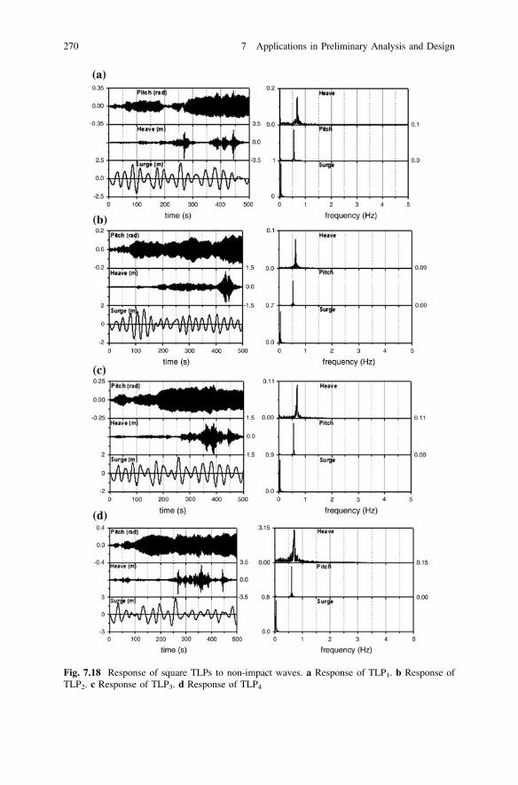
Fig. 7.18 Response of square TLPs to non-impact waves. a Response of TLP1. b Response ofTLP2. c Response of TLP3. d Response of TLP4
270 7 Applications in Preliminary Analysis and Design
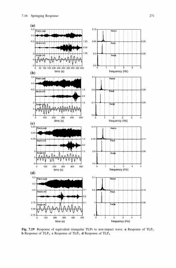
Fig. 7.19 Response of equivalent triangular TLPs to non-impact wave. a Response of TLP1.b Response of TLP2. c Response of TLP3. d Response of TLP4
7.16 Springing Response 271
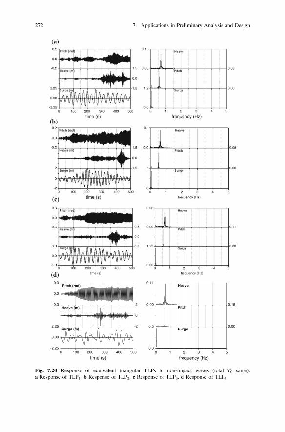
0 1 2 3 4 50.0
0.5 0.00
0.150.00
0.11
Surge
frequency (Hz)
Pitch
Heave
0 100 200 300 400 500-2.25
0.00
2.25 -2
0
2-0.3
0.0
0.3
Surge (m)
time (s)
Heave (m)
Pitch (rad)
(a)
(b)
(c)
(d)
Fig. 7.20 Response of equivalent triangular TLPs to non-impact waves (total T0 same).a Response of TLP1. b Response of TLP2. c Response of TLP3. d Response of TLP4
272 7 Applications in Preliminary Analysis and Design
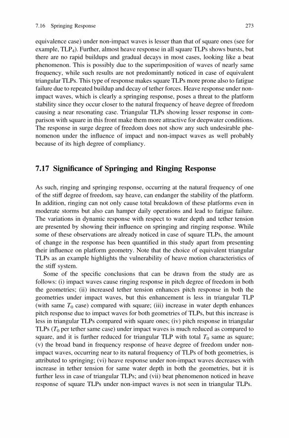
equivalence case) under non-impact waves is lesser than that of square ones (see forexample, TLP4). Further, almost heave response in all square TLPs shows bursts, butthere are no rapid buildups and gradual decays in most cases, looking like a beatphenomenon. This is possibly due to the superimposition of waves of nearly samefrequency, while such results are not predominantly noticed in case of equivalenttriangular TLPs. This type of response makes square TLPs more prone also to fatiguefailure due to repeated buildup and decay of tether forces. Heave response under non-impact waves, which is clearly a springing response, poses a threat to the platformstability since they occur closer to the natural frequency of heave degree of freedomcausing a near resonating case. Triangular TLPs showing lesser response in com-parison with square in this front make them more attractive for deepwater conditions.The response in surge degree of freedom does not show any such undesirable phe-nomenon under the influence of impact and non-impact waves as well probablybecause of its high degree of compliancy.
7.17 Significance of Springing and Ringing Response
As such, ringing and springing response, occurring at the natural frequency of oneof the stiff degree of freedom, say heave, can endanger the stability of the platform.In addition, ringing can not only cause total breakdown of these platforms even inmoderate storms but also can hamper daily operations and lead to fatigue failure.The variations in dynamic response with respect to water depth and tether tensionare presented by showing their influence on springing and ringing response. Whilesome of these observations are already noticed in case of square TLPs, the amountof change in the response has been quantified in this study apart from presentingtheir influence on platform geometry. Note that the choice of equivalent triangularTLPs as an example highlights the vulnerability of heave motion characteristics ofthe stiff system.
Some of the specific conclusions that can be drawn from the study are asfollows: (i) impact waves cause ringing response in pitch degree of freedom in boththe geometries; (ii) increased tether tension enhances pitch response in both thegeometries under impact waves, but this enhancement is less in triangular TLP(with same T0 case) compared with square; (iii) increase in water depth enhancespitch response due to impact waves for both geometries of TLPs, but this increase isless in triangular TLPs compared with square ones; (iv) pitch response in triangularTLPs (T0 per tether same case) under impact waves is much reduced as compared tosquare, and it is further reduced for triangular TLP with total T0 same as square;(v) the broad band in frequency response of heave degree of freedom under non-impact waves, occurring near to its natural frequency of TLPs of both geometries, isattributed to springing; (vi) heave response under non-impact waves decreases withincrease in tether tension for same water depth in both the geometries, but it isfurther less in case of triangular TLPs; and (vii) beat phenomenon noticed in heaveresponse of square TLPs under non-impact waves is not seen in triangular TLPs.
7.16 Springing Response 273
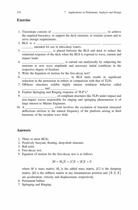
Exercise
1. Triceratops consists of ___________________________________ to achievethe required buoyancy, to support the deck structure, to restrain system and toserve storage requirements.
2. BLS is a ___________________, ___________________, ___________________ intended for use in ultra-deep waters.
3. ___________________ is placed between the BLS and deck to reduce therotational response of the deck when the BLS is exposed to wave, current andimpact loads.
4. ___________________________ is carried out analytically by subjecting thestructure to zero wave amplitude and necessary initial conditions in therespective degree of freedom.
5. Write the Equation of motion for the free-decay test?6. ______________________________ in BLS units results in significant
reduction in the pretension in tethers in comparison with that of TLPs.7. Offshore structures exhibit highly intense nonlinear behavior called
______________ and ________________.8. Explain Springing and Ringing response of TLP’s?9. ______________________ of compliant structures like TLPs under impact and
non-impact waves responsible for ringing and springing phenomenon is oflarge interest to Marine Engineers.
10. A __________________ event involves the excitation of transient structuraldeflections at/close to the natural frequency of the platform arising at thirdharmonic of the incident wave field.
Answers
1. Three or more BLSs.2. Positively buoyant, floating, deep-draft structure.3. Ball joint.4. Free-decay test.5. Equation of motion for the free-decay test is as follows
M þMa½ �€X þ C½ � _X þ ½K�X ¼ 0
where M is mass matrix; Ma is the added mass matrix, [C] is the dampingmatrix, [K] is the stiffness matrix at any instantaneous position and €X; _X;X
� �are acceleration, velocity and displacement, respectively.
6. Permanent ballast.7. Springing and Ringing.
274 7 Applications in Preliminary Analysis and Design

8. Springing is caused in the vertical/bending modes by second-order wave effectsat the sum frequencies; this behavior is common in both mild and severe seastates. Ringing is attributed to strong transient response observed in thesemodes under severe loading conditions triggered presumably by passage of ahigh, steep wave. This transient response further decays to steady state at alogarithmic rate depending on the system damping.
9. Dynamic response.10. Ringing.
Answers 275
References
Adams AJ, Baltrop NDP (1991) Dynamics of fixed Mar Struct. Butterworth-Helneman Ltd.,London
Adrezin R, Bar-Avi P, Benaroya H (1996) Dynamic response of compliant offshore structures-review. J Aerosp Eng 9(4):114–131
Anagnostopoulos SA (1982) Dynamic response of offshore structures to extreme waves includingfluid-structure interaction. Eng Struct 4:179–185
API-RP2A (1989) Recommended practice for planning, designing and constructing fixed offshoreplatforms, 18th edn. American Petroleum Institute, Washington, DC
ASTM (2005) Rainflow counting method. ASTM E 1049–1085Bai Y (2001) Pipelines and risers. Elsevier Ocean Eng book series, vol. 3. Elsevier, AmsterdamBar-Avi P (1999) Nonlinear dynamic response of a tension leg platform. J Offshore Mech Arct
Eng 121:219–226Basim Mekha B, Johnson C, Philip Jose, Roesset M (1996) Implication of tendon modeling on
nonlinear response of TLP. J Struct Eng 122(2):142–149Bathe KJ,Wilson EL (1987) Numerical methods in finite element analysis. Prentice Hall, NewDelhiBea RG, Xu T, Stear J, Ramas R (1999) Wave forces on decks of offshore platforms. J Waterw
Port Coast Ocean Eng 125(3):136–144Bearman PE, Russell MP (1996) Viscous damping of TLP hulls. In: Managed program on
uncertainties and loads on offshore structures (ULOS), Project Report, Imperial CollegeBhattacharyya SK, Sreekumar S, Idichandy VG (2003) Coupled dynamics of Sea Star mini tension
leg platform. Ocean Eng 30:709–737Boaghe OM, Billings SA, Stansby PK (1998) Spectral analysis for non-linear wave forces. J Appl
Ocean Res 20:199–212Booton M, Joglekar N, Deb M (1987) The effect of tether damage on tension leg platform
dynamics. J Offshore Mech Arct Eng 109:186–192Bringham EO (1974) The fast fourier transform. Prentice Hall, Englewood CliffsBuchner B, Bunnik T (2007) Extreme wave effects on deepwater floating structures. In:
Proceedings of offshore technology conference OTC 18493, Houstan, Texas, April 30–May 3Buchner B, Wichers JEW, de Wilde JJ (1999) Features of the state-of-the-art deepwater offshore
basin. In: Proceedings of offshore technology conference OTC 10841, Houstan, Texas, May 3–6Burrows R, Tickell RG, Hames D, Najafian G (1992) Morison wave forces co-efficient for
application to random seas. J Appl Ocean Res 19:183–199Chaudhury G, Dover W (1995) Fatigue analysis of offshore platforms subjected to sea wave
loading. Int J Fatigue 7(1):13–19CAP 437 (2010) Offshore helicopters landing areas: guidance on standards, 6th edn. Civil Aviation
Authority, UKCapanoglu CC, Shaver CB, Hirayama H, Sao K (2002) Comparison of model test results and
analytical motion analyses for buoyant leg structure. In: Proceedings of 12th internationaloffshore and polar engineering conference, Kitakushu, Japan, May 26–31, pp 46–53
© Springer India 2015S. Chandrasekaran, Dynamic Analysis and Design of Offshore Structures,Ocean Engineering & Oceanography 5, DOI 10.1007/978-81-322-2277-4
277

Caughey TK (1960) Classical normal modes in damped linear dynamic systems. J App Mech(ASME) 27:269–271
Chakarabarti SK, Hanna SY (1990) Added mass and damping of a TLP column model. In:Proceedings of offshore technology conference, No. 4643, pp 533–545
Chakrabarti SK (1984) Steady drift force on vertical cylinder—viscous vs potential. Appl OceanRes 6(2):73–82
Chakrabarti SK (2002) The theory and practice of hydrodynamics and vibration. World Scientific,Singapore
Chakrabarti SK (1987) Hydrodynamics of offshore structures: computational mechanics. WITPress, Southampton
Chakrabarti SK (1990) Non-linear method in offshore engineering. Elsevier Science Publisher,The Netherlands
Chakrabarti SK (1994) Offshore structure modeling. World Scientific, SingaporeChandrasekaran S (2013a) Dynamic of ocean structures. Web-based course on National program
on Technology Enhanced Learning, IIT Madras. Available at nptel.ac.in/courses/114106036Chandrasekaran SS (2013b) Ocean structures and materials. Web-based course on National
program on Technology Enhanced Learning, IIT Madras. Available at: nptel.ac.in/courses/114106035
Chandrasekaran S (2013c) Advanced Mar Struct. Web-based course on National program onTechnology Enhanced Learning, IIT Madras. Available at nptel.ac.in/courses/114106037
Chandrasekaran S, Jain AK (2002a) Dynamic behavior of square and triangular offshore tensionleg platforms under regular wave loads. Ocean Eng 29(3):279–313
Chandrasekaran S, Jain AK (2002b) Triangular configuration tension leg platform behavior underrandom sea wave loads. Ocean Eng 29(15):1895–1928
Chandrasekaran S, Jain AK (2004). Aerodynamic behavior of offshore triangular tension legplatforms. In: Proceedings of ISOPE, Toulon, France, pp 564–569
Chandrasekaran S, Pannerselvam R (2009) Offshore structures: materials, analysis, design andconstruction. In: Proceedings of short course on offshore structures and materials, IITM,Chennai, December 14–18, p 156
Chandrasekaran S, Gaurav (2008) Offshore triangular tension leg platform earthquake motionanalysis under distinctly high sea waves. J Ships Offshore Struct 3(3):173–184
Chandrasekaran S, Bhaskar K, Muhammed H (2010). Experimental study on dynamic responsebehavior of multi-legged articulated tower. Proceedins of 29th international conference onocean, offshore and arctic engineering, OMAE 2010, June 6–11, Shanghai, China
Chandrasekaran S, Bhaskar K, Lino H, Brijit R (2010). Dynamic response behavior of multi-legged articulated tower with and without TMD. In: Proceedings of International Conferenceon Mar Technol MARTEC–2010, December 11–12, Dhaka, Bangladesh, pp 131–136
Chandrasekaran S, Chandak NR, Gupta A. (2006) Stability analysis of TLP tethers. Ocean Eng33(3):471–482
Chandrasekaran S, Jain AK, Chandak NR (2004) Influence of hydrodynamic coefficients in theresponse behavior of triangular TLPs in regular waves. Ocean Eng 31:2319–2342
Chandrasekaran S, Jain AK, Chandak NR (2006) Seismic analysis of offshore triangular tensionleg platforms. Int J Struct Stab Dyn 6(1):97–120
Chandrasekaran S, Jain AK, Chandak NR (2007) Response behavior of triangular tension legplatforms under regular waves using stokes nonlinear wave theory. J Waterw Port Coast OceanEng (ASCE) 133(3):230–237
Chandrasekaran S, Jain AK, Gupta A (2007) Influence of wave approach angle on TLP’s response.Ocean Eng 8-9(34):1322–1327
Chandrasekaran S, Jain AK, Gupta A, Srivastava A (2007) Response behavior of triangulartension leg platforms under impact loading. Ocean Eng 34:45–53
Chandrasekaran S, Seeram M, Jain AK, Gaurav M (2010) Dynamic response of offshoretriceratops under environmental loads. In: Proceedings of international conference on MarTechnol MARTEC, December 11–12, Dhaka, Bangladesh, pp 61–66
278 References
Chandrasekaran S, Sharma A, Srivastava S (2007) Offshore triangular TLP behavior usingdynamic Morison equation. J Struct Eng 34(4):291–296
Chandrasekaran S, Sundaravadivelu R, Pannerselvam R, Madhuri S (2011) Experimentalinvestigations of offshore triceratops under regular waves. In: Proceedings of 30th internationalconference on ocean, offshore and arctic engineering, OMAE, 19–24 June 2011, Rotterdam,The Netherlands
Chandrasekaran S, Sundaravadivelu R, Pannerselvam R, Madhuri S, Shyamala Varthini D (2011)Experimental investigations of offshore triceratops under regular waves. In: Proceedings of30th international conference on ocean, offshore and arctic engineering, OMAE, June 19–24,Rotterdam, The Netherlands, 49826
Chandrsaekaran S, Bhattacharyya SK (2011) Analysis and design of offshore structures. HRDCenter for Offshore and Plant Engineering (HOPE), Changwon National University, Republicof Korea, p 285
Charles WN, Robert CW, Capanoglu C (2005) Triceratops: an effective platform for developingoil and gas fields in deep and ultra deep water. In: Proceedings of 15th international offshoreand polar engineering conference, June 19–24, Seoul, Korea, pp 133–139
Chen X, Ding Y, Zhang J, Liagre P, Neidzwecki J, Teigen P (2006) Coupled dynamic analysis of amini TLP: comparison with measurements. Ocean Eng 33:93–117
Choi Han S, Lou, Jack YK (1991) Nonlinear behavior of an articulated offshore loading platform.Appl Ocean Res 13(2):63–74
Chopra AK (2003) Dynamics of structures: theory and applications to earthquake engineering, 2ndedn. Person Education, Singapore
Clauss GF, Birk L (1996) Hydrodynamic shape optimization of large offshore structures. J ApplOcean Res 18:157–171
Clauss GT et al (1992) Offshore structures: conceptual design and hydromechanics, vol 1.Springer, London
Copple RW, Capanoglu CC (1995) A buoyant leg structure for the development of marginal fieldsin deep water. In: Proceedings of fifth international offshore and polar engineering conference,June 16–11,The Hague, The Netherlands, p 163
Dawson TH (1983) Offshore structural engineering. Prentice-Hall, Englewood Cliffsde Boom William C, Pinkster Jo A, Tan PSG (1984) Motion and tether force prediction of a
TLP. J Waterw Port Coast Ocean Eng 110(4):472–486Demirbilek Z (1990) Design formulae for offset, set down and tether loads of a tension leg
platform (TLP). Ocean Eng 17(5):517–523Devon R, Jablokow K (2010) Teaching FEED. In: Proceedings of mid-atlantic ASEE conference,
October 15–16, Villanova University, Pennsylvania, USADNV (1982) Rules for the design, construction and inspection of offshore structures. Det Norske
Veritas, OsloDOE-OG (1985) Offshore installation: guidance on design and construction. Department of
Energy, LondonErtas A, Eskwaro-Osire S (1991) Effect of damping and wave parameters on offshore structure
under random excitation. Nonlinear Dyn 2:119–136Ertas A, Lee JH (1989) Stochastic response of tension leg platform to wave and current forces.
J Energy Resour Technol 111:221–230Faltinsen OM (1990) Sea loads on ships and offshore structures. Cambridge University Press,
New YorkFaltinsen OM, Newman JN, Vinje T (1995) Nonlinear wave loads on a slender vertical cylinder.
J Fluid Mech 289:179–198Gadagi MM, Benaroya H (2006) Dynamic response of an axially loaded tendon of a tension leg
platform. J Sound Vib 293:38–58Gaurav, Sharma A (2008) Influence of varying inertia coefficient and wave directionality on TLP
geometry. In: Proceedings of ISOPE, November 2008, Bangkok, Thailand, pp 255–261Gerwick BC Jr (1986) Construction of offshore structures. Wiley, New York
References 279

Graff WJ (1981) Introduction to offshore structures. Gulf Publishing Co., HoustonGraff WJ (1981) Introduction to offshore structures: design, fabrication and installation. Gulf
Publishing Co., TokyoGuo B, Song S, Chacko J, Ghalamber A (2005) Offshore pipelines. Gulf Professional Publishing,
MAGurley Kurtis R, Ahsan Kareem (1998) Simulation of ringing in offshore systems under viscous
loads. J Eng Mech ASCE 124(5):582–586Gusto MSC (2010) The exploration market. Inside 15:4–7Halkyard JE, Davies RL, Glanville RS (1991) The tension buoyant tower: a design for deep water.
23rd annual offshore technology conference, OTC 6700, May 69,Houston, Texas, pp 41–55Hancock JW, Gall DS (1985) Fatigue under narrow and broad band stationary loading. Final
report of cohesive program of R&D in fatigue of offshore structures, Marine Tech. DirectorateLtd., Texas, USA
Haritos N (1985) Modeling the response of tension leg platforms to the effects of wind usingsimulated traces. Math Comput Simul 27:231–240
Harvy JF (1985) Theory and design of pressure vessels. Van Nostrand Reinhold Co, New YorkHelvacioglu IH, Incecik A (2004) Dynamics of double articulated towers, integrity of offshore
structures, vol 4. Elsevier, LondonHitchings GA, Bradshaw H, Labiosa TD (1976) Planning and execution of offshore site
investigations for North Sea gravity platform. In: Proceedings of offshore technologyconference, Paper No. 2430
Hoeg K (1976) Foundation engineering for fixed offshore structures. In: Proceedings of firstinternational conference behaviour of offshore structures, vol 1, pp 39–69
Hove K, Foss I (1974) Quality assurance for offshore concrete gravity structures. In: Proceedingsof Offshore Technology Conference, Paper No. 2113
HSE (2010) Offshore helideck design guidelines: health & safety executive. John Burt AssociatesLtd, UK
Hsu HT (1981) Applied offshore structural engineering. Gulf Publishing Co., HoustonHumphries JA, Walker DH (1987) Vortex excited response of large scale cylinders in shear flow.
In: Proceedings of Sixth OMAE, vol 2, Houston, TX, pp 139–143Islam N, Ahmad S (2003) Nonlinear seismic response of articulated offshore tower. Def Sci J 53
(1):105–113Issacson M, Det St Q (1982) Non-linear wave effects on fixed and floating bodies. J Fluid Mech
120:267–281Iwasaki H (1981) Preliminary design study of tension leg platform. MIT UniversityJayalekshmi R, Sundaravadivelu R, Idichandy VG (2010) Dynamic analysis of deep water tension
leg platforms under random waves. J Offshore Mech Arct Eng 132(4):041605Jefferys ER, Patel MH (1982) Dynamic analysis models of tension leg platforms. J Energy Resour
Technol 104:217–223Jefferys ER, Rainey RCT (1994) Slender body models of TLP and GBS ‘ringing’. BOSS,
McGraw-Hill Inc, New YorkJoseph A, Idichandy VG, Bhattacharyya SK (2004) Experimental and numerical study of coupled
dynamic response of a mini tension leg platform. J Offshore Mech Arct Eng 126(4):318–330Kam JCP, Dover WD (1988) Fast fatigue assessment procedure under random time history. Proc
Inst Civil Eng Part 2 85:689–700Kam JCP, Dover WD (1989) Advanced tool for fast assessment of fatigue under offshore random
wave stress history. Proc Inst Civil Eng Part 2 87:539–556Kawanishi T, Katoh W, Furuta H (1987) Tension leg platform earthquake motion analysis. Oceans
19:543–547Kawanishi T, Ohashi S, Takamura H, Koboyashi H (1993) Earthquake response of tension leg
platform under unbalanced initial tension. In: Proceedings of ISOPE, Singapore, pp 319–325Ker W-K, Lee C-P (2002) Interaction of waves and a porous tension leg platform. J Waterw Port
Coast Ocean Eng 128(2):88–95
280 References
Kim C-H, Zou J (1995) A universal linear system model for kinematics and forces affected bynonlinear irregular waves. Int J Offshore Polar Eng 5(3):166–170
Kim C-H, Kim MH, Liu YH, Zhao CT (1994) Time domain simulation of nonlinear response of acoupled TLP system. Int J Offshore Polar Eng 4(4):281–291
Kim C-H, Lee C-H, Goo J-S (2007) A dynamic response analysis of tension leg platformsincluding hydrodynamic interaction in regular waves. Ocean Eng 34:1680–1689
Kim C-H, Zhao CT, Zou J, Xu Y (1997) Springing and ringing due to laboratory-generatedasymmetric waves. Int J Offshore Polar Eng 7(1):30–35
Kjeldsen SP, Myrhaug D (1979) Wave-wave interactions and wave-current interactions in deepwater. In: Proceedings of 5th POAC Conference, Trondheirn, Norway, vol. III, p 179
Klaus-Jurgen B, Wilson EL (1987) Numerical methods in finite element analysis, 2nd edn.Pearson Education, Singapore
Kobayashi M, Shimada K, Fujihira T (1987) Study on dynamic responses of a TLP in waves.J Offshore Mech Arct Eng 109:61–66
Kurian et al (2008) Parametric study of TLPs subjected to random waves. In: Proceeding ofinternational conference on construction and building technology, Kuala Lumpur, Malaysia,pp 1–9
Kurian VJ, Idichandy VG, Ganapathy C (1993) Hydro dynamic response of tension leg platforms:a model. Exp Mech 33(3):212–217
Leffler William WL, Pattarozzi R, Sterling G (2011) Deep-water petroleum: exploration andproduction. Pennwell Corp., Oklahama, p 350
Li Y, Liu Y, Teng B (2006) Porous effect parameter of thin permeable plates. Coast Eng 48(4):309–336
Love AEH (1994) Mathematical theory of elasticity. Dover Publications, New YorkLow YM (2009) Frequency domain analysis of a tension leg platform with statistical linearization
of the tendon restoring forces. Mar Struct 22:480–503Malenica S, Molin B (1995) Third-harmonic diffraction by a vertical cylinder. J Fluid Mech
302:203–229Marthinsen T, Winterstein SR, Ude TC (1992) TLP fatigue due to second-order springing.
Probabilistic methods and structural and geotechnical reliability. In: Proceedings of specialtyconference, pp 455–458
Mather A (2000) Offshore engineering: an introduction, 2nd edn. Witherby & Co Ltd., LondonMatsuishi M, Endo T (1968) Fatigue of metals subjected to varying stresses. Jpn Soc Mech Eng
3:37–40McCamy RC, Fuchs RA (1954). Wave force on piles: a diffraction theory. Technical
Memorandum, No. 69, Beach Erosion Board, US. Army Corps of Engineers, Washington, DCMercier JA (1982) Evolution of tension leg platform technology. In: Proceedings of 3rd
international conference on the behaviour of offshore structures, MITMercier RS (1997) Mars tension leg platform: use of scale model testing in the global design. In:
Proceedings of offshore technology conference, OTC 8354-MS, May 5–8, Houston, TexasMichel WH (1999) Sea spectrum revisited. Mar Technol 36(4):211–227Moe G, Verley RLP (1980) Hydrodynamic damping of offshore structures in wave and currents.
Offshore technology conference, 12th Annual OTC, Houston, Texas, pp 37–44Morison JR, O’Brien MP, Johanson JW, Shaaf SA (1950) The forces exerted by surface waves on
pile. Trans AMIE 189:149–154Muhuri PK, Gupta AS (1983) Stochastic stability of tethered buoyant platforms. Ocean Eng 10
(6):471–479Munkejord T (1996) The Heidrun TLP and concept development for deep water. In: Proceedings
of ISOPE, May, Los Angeles, USA, pp 1–11Naess A, Moan T (2013) Stochastic dynamics of marine structures. Cambridge University Press,
New YorkNagamani K, Ganapathy C (2000) Dynamic response of three leg articulated tower. Ocean Eng
27:1455–1471
References 281

Natvig BJ (1996) TLP installation without motion compensation. In: Proceedings of ISOPE, LosAngeles, CA, USA, 1, pp 228–231
Natvig BJ (1994) A proposed ringing analysis model or higher order tether response. In:Proceedings 4th international offshore and polar engineering conference, ISOPE, Golden, CO,pp 40–51
Natvig BJ, Vogel H (1995)TLP design philosophy—past, present, future. In: Proceedings ofinternational conference offshore and polar engineers, The Hague, pp 64–69
Neelamani S, Muni Reddy MG (2002) Wave forces on a vertical cylinder defenced by a perforatedvertical and inclined barriers. Indian J Mar Sci 31(3):179–187
Neelamani S, Uday Bhaskar N, Vijayalakshmi K (2002) Wave forces on a seawater intake caisson.Ocean Eng 29(10):1247–1263
Neville AM (1997) Properties of concrete, 4th edn. Wiley, New YorkNiedzwecki JM, Van de Lindt JW, Gage JH, Teigen PS (2000) Design estimates of surface wave
interaction with compliant deepwater platforms. Ocean Eng 27:867–888Nobuyoshi Y (1976) Experimental and theoretical study of a tension leg platform in deep water.
In: Proceedings of offshore technology conference, OTC 2690-MS, May 3 6, Houston, TexasNordgren RP (1987) Analysis of high frequency vibration of tension leg platforms. J Offshore
Mech Arct Eng 109:119–125NPD (1985) Regulation for structural design of load-bearing structures intended for exploitation of
petroleum resources. Norwegian Petroleum Directorate, OsloOCS (1980) Requirements for verifying the structural integrity of OCS platforms. United States
Geologic Survey, National Centre, RestonPaik JK, Thayamballi AK (2007) Ship-shaped offshore installations: design, building and
operations. Cambridge University Press, New YorkPaik I, Roesset JM (1996) Use of quadratic transfer functions to predict response of tension leg
platforms. J Eng Mech 122(9):882–889Patel MH (1989) Dynamics of offshore structures. Butterworth, LondonPatel M, Witz JA (1991) Compliant offshore structures. Butterworth-Heinemann Ltd., OxfordPerryman SR, Horton EE, Halkyard JE (1995) Tension buoyant tower for small fields in deep
waters. Offshore technology conference, OTC 7805, May 1–4, Houston, Texas, pp 13–22Pilotto BM, Ronalds, BF, Stocker R (2002) Dynamic response of shallow water mono-pod
platforms. In: Proceedings of international conference on offshore mechanics and arcticengineering, Oslo, Norway, 1, pp 113–120
Pilotto BM, Ronalds BF, Stocker R (2003) Nonlinear dynamic analysis with deterministic andrandom seas. Oceans Conf Rec (IEEE) 5:2908–2915
Pilotto BM, Ronalds BF (2003) Dynamic behavior of minimum platforms under random loads. In:Proceedings of international conference on offshore mechanics and arctic engineering,Cancum, Mexico, 1, pp 441–449
Popovics JS, Zemajtis J, Shkilnik I (2008) Study on static and dynamic modulus of elasticity ofconcrete. American Concrete Institute, CRC Report
Reddy DV, Arockiasamy M (1991) Offshore Structures, vol I. Kriger Publishing Co., MalabarRijken OR, Niedzwecki JM (1991) A knowledge base approach to the design of tension leg
platform. Center for Offshore Technology, Offshore Technology Research Center, Texas,pp 24–100
Roark RJ, Yooung WC (1989) Formula for stress and strain, 6th edn. McGraw Hill Inc, New YorkRobert WC, Capanoglu CC (1995) Buoyant leg structure for the development of marginal fields in
deep water. In: Proceedings of International Offshore and Polar Engineering Conference, June11–16, The Hague, The Netherlands, p 163
Ney R, Andrade RFM, Batista RC (1992) Dynamic response analysis of small-scale model tensionleg platform. Mar Struct 5:491–513
Sadehi K (1989) Design and analysis of marine structure. Khaje Nasir Toosi University ofTechnology, Tehran
282 References
Sadehi K (2001) Coasts, ports and offshore structures engineering. Power and Water University ofTechnology, Tehran
Sadehi K (2007) Offshore and petroleum platforms for cyprus oil/gas fields. J Soc Appl Sci2(4):1–16
Sankarbabu K, Sannasiraj SA, Sundar V (2007) Interaction of regular waves with a group of dualporous circular cylinders. Appl Ocean Res 29(4):180–190
Sarpkaya T, Isaacson M (1981) Mechanics of wave forces on offshore structures. Van NostrandReinhold, New York
Seeram M (2013) Nonlinear dynamic behaviour of offshore triceratops. PhD thesis, Indian Instituteof Technology Madras, p 145
Shaver CB, Capanoglu CC, Serrahn CS (2001) Buoyant leg structure preliminary design,constructed cost and model test results. In: Proceedings 11th international offshore and polarengineering conference, Stavanger, Norway, June 17–22, pp 432–439
Shinozula M (1983) Basic analysis of structural safety. J Struct Div ASCE 109(3):721–740Soding H, Blok JJ, Chen HH, Hagiwara K, Issacson M, Jankowski J, Jefferys ER, Mathisen J,
Rask I, Richer JP, Romeling JU, Varsta P (1990) Environmental forces on offshore structures:a state-of-art review. Mar Struct 3:59–81
Son S (2006) Design of ocean platforms against ringing response. MS thesis, MechanicalEngineering Department, Texas Tech University, Lubbock, TX, USA
Song H, Tao L (2007) Short-crested wave interaction with a concentric porous cylindricalstructure. Appl Ocean Res 29(4):199–209
Stansberg CT, Ormberg H, Oritsland O (2002) Challenges in deep water experiments: hybridapproach. J Offshore Mech Arct Eng 124:90–96
Stoke’s GG (1880) On the theory of oscillatory waves. Math Phys Pap 1:225–228Subramanaim KV, Popovics JS, Shah SP (2000) Determining elastic properties of concrete using
vibration resonance frequencies of standard test cylinders. Cem Concr Aggreg (ASTM)22(2):81–89
Tabeshpour MR, Golafshani AA, Seif MS (2006) Comprehensive study on the results of tensionleg platform responses in random sea. J Zhejiang Univ Sci 7(8):1305–1317
Tromans P, Swan C, Masterton S (2006) Nonlinear potential flow forcing: the ringing of concretegravity based structures. Research Report No. 468, Ocean Wave Engineering Ltd, Health &Safety Executive Publication, Norwich, UK
Ude TC, Winterstein SR, Marthinsen T (1994) Volterra models for ocean structures: extreme andfatigue reliability. J Eng Mech ASCE 120(6):1369–1385
Vannucci P (1996) Simplified optimal design of tension leg platform TLP. Struct Optim12:265–268
Venkataramana K, Toyoda S, Kawano K (1993) Dynamics of TLPs under current and earthquakeforces. In: Proceedings of ISOPE, Singapore, pp 341–344
Vickery PJ (1990) Wind and wave loads on a tension leg platform: theory and experiment. WindEng Ind Aerodyn 36:905–914
Vickery PJ (1995) Wind induced response of tension leg platform: theory and experiments. StructEng 121(4):651–663
Vijayalakshmi K, Neelamani S, Sundaravadivelu R, Murali K (2007) Wave run up on a concentrictwin perforated circular cylinder. Ocean Eng 34(2):327–336
Vijayalakshmi K, Sundaravadivelu R, Murali K, Neelamani S (2008) Hydrodynamics of aconcentric twin perforated circular cylinder system. J Waterw Port Coast Ocean Eng134(3):166–177
Wang K-H, Ren X (1994) Wave interaction with a concentric porous cylinder system. Ocean Eng21(4):343–360
White NC, Copple WR, Capanoglu C (2005) Triceratops: an effective platform for developing oiland gas fields in deep and ultra-deep water. In: Proceedings of 15th international offshore andpolar engineering conference, June 19–24, Seoul, Korea, pp 133–139
References 283

William AN, Li W (1998) Wave interaction with a semi-porous cylindrical breakwater mounted ona storage tank. Ocean Eng 25(2–3):195–219
William AN, Li W, Wang K-H (2000) Water wave interaction with a floating porous cylinder.Ocean Eng 27(1):1–28
Williams AN, Li W (2000) Water wave interaction with an array of bottom-mounted surface-piercing porous cylinders. Ocean Eng 27(8):841–866
Wilson James F (1984) Dynamics of offshore structures. Wiley Inter Science Publications,New York
Winterstein SR (1988) Nonlinear vibration models for extremes and fatigue. J Eng Mech ASCE114(10):1772–1790
Wirsching P, Ortiz PK (2006) Random vibrations: theory and practice. Dover, NewYorkWirsching PH, Light MC (1980) Fatigue under wide band random loading. J Struct Div ASCE
106:1593–1607Witz JA, Patel MH, Harrison JH (1986) On the hydrodynamics of semisubmersibles with
articulated members. Proc Roy Soc London Ser A Math Phys Sci 403:81–109Yan F, Zhang D, Sun L, Dai Y (2009) Stress verification of a TLP under extreme wave
environment. J Mar Sci Appl 8:132–136Yoneya T, Yoshida K (1982) The dynamics of tension leg platforms in waves. J Energy Resour
Technol 104:20–28Yoshida K, Ozaki M, Oka N (1984) Structural response analysis of tension leg platforms. J Energy
Resour 106:10–17Young AG, Kraft LM, Focht JA (1975) Geotechnical considerations in foundation design of
offshore gravity structures. In: Proceedings of offshore technology conference, Paper No. 2371Zeng et al (2007) Parametric studies of tension leg platform with large amplitude motions. In:
Proceedings 17th international offshore and polar engineering conference, Lisbon, Portugal,pp 202–209
Zhao F, Bao W, Kinoshita T, Itakura H (2009) Interaction of waves and a porous cylinder with aninner horizontal porous plate. Appl Ocean Res 32(2):252–259
Zhong Z, Wang KH (2006) Solitary wave interaction with a concentric porous cylinder system.Ocean Eng 33(7):927–949
284 References

Index
AAccidental load, 25, 54Aerodynamic admittance function, 27, 28Airy’s wave theory, 30, 244, 258Amplitude amplification, 203–207Analytical model, 259Analytical studies, 244Applications in design, 243Applications in preliminary analysis, 243Arctic regions, 1, 39Articulated tower, 9
BBlockage factor, 176Bottom-supported structures, 3Bullwinkle steel jacket, 5Buoyancy dominant, 11Buoyant leg structures (BLSs), 16–19, 243,
274Buoyant tower, 16–18
CCantilever, 101Caughey damping, 161Chappelear numerical theory, 32Cnoidal theory, 32Compliant-type structures, 4CONDEEP (concrete deep-water) structure, 6Coulomb damping, 155Crack propagation, 238
DD'Alembert's principle, 69Damped vibration
forced, 78free, 69–77, 83
DampingCoulomb damping, 71, 72, 155, 170
critical damping, 75, 76over-damping, 76under-damping, 74viscous, 71viscous damping, 71, 155
Damping matrix, 158, 159, 163–168, 248,264–274
classical damping, 166super positioning, 158, 159, 163–169, 248,
263Damping models
Caughey damping, 162Rayleigh Damping, 157
Dead load, 42Dean's stream function theory, 32Degree of freedom, 64, 264Drag force, 173, 201Dunkerley's method, 95, 105, 139Dynamic loads, 63Dynamic matrix, 94Dynamics of triangular TLP, 263
damping matrix, 263mass matrix, 263stiffness matrix, 263, 264
EEarthquake loads, 36Eigenvalue problem, 93–95, 101Empirical prediction, 249Energy method, 68Environmental forces , 25–54Environmental loads, 22, 25, 55Equation of motion, 66, 69, 85, 89, 91, 93, 121,
123Evaluation of damping, 169Evolution of Platform Geometry, 257Exceedance, 215, 231, 232Experimental damping, 169
© Springer India 2015S. Chandrasekaran, Dynamic Analysis and Design of Offshore Structures,Ocean Engineering & Oceanography 5, DOI 10.1007/978-81-322-2277-4
285

Experimental investigationsperforated cylinders, 181perforated TLP, 181, 185
Evolution of platform geometry, 257Experimental studies, 250
FFabrication, 12, 15–17, 22, 48–50Failures
buckling, 40cracking, 40crushing, 40spalling, 40
Fatigueanalysis, 228assessment, 225broadband, 234deterministic, 231failure, 225loading, 224, 228narrowband, 233SN approach, 225spectral, 232time domain, 229
Fatigue and fracture, 224Floating, Storage and Regasification Units
(FSRUs), 19Floating platform, 13Floating production, storage and offloading
systemssee FPSO
Flow in deep waters, 175Fluid structure interaction, 173Forced vibration, 78
damped, 80un-damped, 78, 79
FPSO, 3, 4, 11, 13, 14Fracture, 224Free-decay studies, 247Free-floating studies, 247Free heave acceleration, 187Free surge acceleration, 187Free vibration
damped, 70–77un-damped, 64, 65, 69, 84
Free vibration response, 243Front-end engineering design (FEED), 2Froude-Krylov theory, 35–37
GGravity-based structures, 256Gravity platform, 5Guyed tower, 8
HHalf power bandwidth method, 78Hibernia gravity base structure, 7Horizontal cylinders, 176
in shear flow, 176in uniform flow, 176
Horizontal velocityvariation, 195–197
Hot spot stresses, 228Hydrodynamic response, 173, 199
IIce and snow loads, 39Impact load, 43Influence coefficients, 91
JJacket platform, 4Jacket platform complex, 4
LLaunch-upending, 53Launch barge and jacket, 53Lena Guyed Tower, 8Lifting forces, 49Limit state function, 223Linear or first-order theory
see Airy's wave theory, 30Load spectrum, 204, 209, 240
MMarine growth, 41, 56Mass, 41Mass matrix, 263Mass proportional damping, 157, 264Mathematical development, 258Mathematical model, 65
multi-degrees-of-freedom model, 89single-degree-of-freedom model, 66two-degrees-of-freedom model, 83
Matrix iteration, 95Miner's rule, 227Mode superposition, 97Mode truncation, 98Model details, 245Motion of floating objects, 52
NNew structural forms, 244Newton's law of motion, 67Numerical models, 189, 195Numerical simulations, 192Numerical studies, 199
286 Index
OOffshore instalations
purposes, 3Offshore platforms
analysis, 46new-generation, 15types, 2
Offshore triceratops, 244–245, 249, 250, 254Oil exploration, 3
PPerforated cylinders
experimental investigations, 181numerical studies, 177, 189
Perforated offshore members, 173–199Perforated TLP model, 185Perforations, 185–189Principal modes of vibration, 84
RRainflow counting, 229Rayleigh-Ritz method, 99Rayleigh damping, 159Rayleigh method, 68Reliability
advantages, 220levels, 219long-term, 218methods, 213, 216, 220
Reliability framework, 213Response amplitude operators (RAOs)
heave RAO, 188, 252pitch/roll RAO, 255surge/sway RAO, 250, 254
Response processauto-covariance, 207mean value, 205
Response spectrum, 204, 208–210, 240Return period, 212Ringing response, 265
SSafety and reliability, 213Scaled model, 243Semi-submersible, 13Skidding, 50Solitary wave theory, 32Spar platform, 14Spatial definition, 228Spring—mass system, 85Springing and ringing, 256–273Springing response, 269
Steady-state response, 82Steel structures, 45Stiffness matrix, 264Stiffness proportional damping, 157Stochastic dynamics, 203–242Stochastic load process, 204Stochastic models, 210
advanced FOSM, 222FOSM method, 221
Stochastic process, 210Stodola's method, 96Stokes fifth-order theory, 32Stress concentration factor, 238Structural damping, 156Structural dynamics, 63–147Structural form, 3, 35
TTemplate-type structures, 4Tension leg platform
analytical model, 259dynamics, 263hydrodynamic forces on, 262
Tension leg platform, 8, 12, 21, 22, 35, 179Tethers, 8, 12, 16, 19Time domain fatigue analysis
see Tension leg platformTransportation forces, 52Triceratops
components, 250free-floating, 249tethered, 18, 19, 243, 249, 274
UUltimate limit state, 46Ultra-deep waters, 7, 15, 17, 243, 244, 249Undamped vibration, 69Up-Crossing approach, 216
VVertical cylinders, 174
WWave approach angles, 250–255Wave directionality effects, 250Wave flume, 245Wave forces, 177, 179Wave–structure interaction, 177Wave theories, 31, 37Weight dominant, 11Wind force, 26
Index 287


