University of Maryland College ParkInstitute for Advanced Computer Studies TR{92{61Department of Computer Science TR{2908SRRIT|A FORTRAN Subroutineto Calculate the Dominant Invariant Subspaceof a Nonsymmetric Matrix�Z. BaiyG. W. StewartzMay, 1992ABSTRACTSRRIT is a FORTRAN program to calculate an approximate orthonor-mal basis for a dominant invariant subspace of a real matrix A by themethod of simultaneous iteration [12]. Speci�cally, given an integer m,SRRIT attempts to compute a matrix Q with m orthonormal columnsand real quasi-triangular matrix T of order m such that the equationAQ = QTis satis�ed up to a tolerance speci�ed by the user. The eigenvalues of Tare approximations to the m largest eigenvalues of A, and the columnsof Q span the invariant subspace corresponding to those eigenvalues.SRRIT references A only through a user provided subroutine to formthe product AQ; hence it is suitable for large sparse problems.�This report is available by anonymous ftp from thales.cs.umd.edu in the directorypub/reports. The program is available in pub/srrityDepartment of Mathematics, University of Kentucky, Lexington, KY 40506.zDepartment of Computer Science and Institute for Advanced Computer Studies, Universityof Maryland, College Park, MD 20742. This work was supported in part by the National ScienceFoundation under Contract Number CCR9115586.

SRRIT|A FORTRAN Subroutineto Calculate the Dominant Invariant Subspaceof a Nonsymmetric Matrix�Z. BaiyG. W. StewartzAbstractSRRIT is a FORTRAN program to calculate an approximate orthonor-mal basis for a dominant invariant subspace of a real matrix A by themethod of simultaneous iteration [12]. Speci�cally, given an integer m, SR-RIT attempts to compute a matrix Q with m orthonormal columns andreal quasi-triangular matrix T of order m such that the equationAQ = QTis satis�ed up to a tolerance speci�ed by the user. The eigenvalues of Tare approximations to the m largest eigenvalues of A, and the columns ofQ span the invariant subspace corresponding to those eigenvalues. SRRITreferences A only through a user provided subroutine to form the productAQ; hence it is suitable for large sparse problems.1. DescriptionThe program described in this paper is designed primarily to solve eigenvalueproblems involving large, sparse nonsymmetric matrices. The program attemptsto calculate a set of the largest eigenvalues of the matrix in question. In additionit calculates a canonical orthonormal basis for the invariant subspace spanned byeigenvectors and principal vectors corresponding to the set of eigenvalues. Noexplicit representation of the matrix is required; instead the user furnishes a sub-routine to calculate the product of the matrix with a vector.�The report is available by anonymous ftp from thales.cs.umd.edu in the directorypub/reports. The program is available in pub/srrit. Earlier version appeared as Techni-cal Report TR-154, Department of Computer Science, University of Maryland, 1978.yDepartment of Mathematics, University of Kentucky, Lexington, KY 40506.zDepartment of Computer Science and Institute for Advanced Computer Studies, Universityof Maryland, College Park, Maryland 20742. This work was supported in part by the NationalScience Foundation under Contract Number CCR9115586.1

2 SRRIT: Simultaneous IterationSince the programs do not produce a set of eigenvectors corresponding to theeigenvalues computed, it is appropriate to begin with a mathematical descriptionof what is actually computed and how the user may obtain eigenvectors fromthe output if they are required. Let A be matrix of order n with eigenvalues�1; �2; : : : ; �n ordered so thatj�1j � j�2j � : : : � j�nj:An invariant subspace of A is any subspace Q for whichx 2 Q =) Ax 2 Q;i.e., the subspace is transformed into itself by the matrix A.If Q is an invariant subspace of A and the columns of Q = (q1; q2; : : : ; qm) forma basis for Q, then Aqi 2 Q, and hence Aqi can be expressed as linear combinationof the columns of Q; i.e., there is an m-vector ti such that Aqi = Qti. SettingT = (t1; t2; : : : ; tm);we have the relation AQ = QT: (1)In fact the matrix T is just the representation of the matrix A in the subspace Qwith respect to the basis Q.If x is an eigenvector of T corresponding to the eigenvalue �, then it followsfrom (1) and the relation Tx = �x thatA(Qx) = �(Qx); (2)so that Qx is an eigenvector of A corresponding to the eigenvalue �. Thus theeigenvalues of T are also eigenvalues of A. Conversely, any eigenvalue of A whoseeigenvector lies in Q is also an eigenvector of T . Consequently, there is a one-onecorrespondence of eigenvectors of T and eigenvectors of A that lie in Q.If j�ij > j�i+1j, then there is a unique dominant invariant subspace Qi corre-sponding to �1; �2; : : : ; �i. When Qi and Qi+1 exist, Qi � Qi+1. SRRIT attemptsto compute a nested sequence of orthonormal bases of Q1;Q2; : : : ;Qm. Specif-ically, if all goes well, the subroutine produces a matrix Q with orthonormalcolumns having the property that if j�ij > j�i+1j then q1; q2; : : : ; qi span Qi.The case where �i�1 and �i are a complex conjugate pair, and hence j�i�1j =j�ij, is treated as follows. The matrix Q is calculated so that the matrix T in ( 1)

SRRIT: Simultaneous Iteration 3is quasi-triangular; i.e., T is block triangular with 1 � 1 and 2 � 2 blocks on itsdiagonal. The structure of a typical quasi-triangular matrix is illustrated belowfor m = 6: 0BBBBBBBB@ � � � � � �0 � � � � �0 � � � � �0 0 0 � � �0 0 0 0 � �0 0 0 0 � � 1CCCCCCCCA :The 1�1 blocks of T contain the real eigenvalues of A and the 2�2 blocks containconjugate pairs of complex eigenvalues. This arrangement enables us to workentirely with real numbers, even when some of the eigenvalues of T are complex.The existence of such a decomposition is a consequence of Schur's theorem [11].The eigenvalues of the matrix T computed by the program appear in descend-ing order of magnitude along its diagonal. For �xed i, let Qji = (q1; q2; : : : ; qi) andlet T �ji be the leading principal submatrix of T of order i. Then if the ith diagonalentry of T does not begin a 2� 2 blocks, we haveAQji = QjiT �ji:Thus the �rst i columns of Q span the invariant subspace corresponding to the�rst i eigenvalues of T . When j�ij > j�i+1j this is the unique dominant invariantsubspace Qi, When j�ij = j�i+1j the columns of Qji span a dominant invariantsubspace; but it is not unique, since there is no telling which comes �rst, �i or�i+1.Any manipulations of A within the subspace Q corresponding to Q can beaccomplished by manipulating the matrix T . For example,AkQ = QT k;so that if f(A) is any function de�ned by a power series, we havef(A)Q = Qf(T ):If the spectrum of A that is not associated with Q is negligible, considerablework can be saved by working with the generally much smaller matrix T in thecoordinate system de�ned by Q. If explicit eigenvectors are desired, they maybe obtained by evaluating the eigenvectors of T and appling (2). The programSTREVC in LAPACK [1] will evaluate the eigenvectors of a quasi-triangular matrix.

4 SRRIT: Simultaneous Iteration2. UsageSRRIT is a subroutine in ANSI FORTRAN 77 to calculate the basis for Qmdescribed in Section 1. The calling sequence for SRRIT isCALL SRRIT ( N, NV, M, MAXIT, ISTART, Q, LDQ, AQ, LDA, T, LDT,WR, WI, RSD, ITRSD, IWORK, WORK, LWORK, INFO, EPS )withN (input) INTEGERThe order of the matrix A.NV (input) INTEGERNV is the size of the leading invariant subspace of A that the userdesired.M (input) INTEGERM is the size of iteration space (NV � M � N).MAXIT (input) INTEGERMAXIT is an upper bound on the number of iterations the program isto execute.ISTART (input) INTEGERISTART speci�es whether user supplies an initial basis Q.� 0, Q is initialized by the program.= 1, starting Q has been set in the input but is not orthonormal.> 1, starting Q has been set in the input and is orthonormal.Q (input/output) REAL array, dimension( LDQ, M )On entry, if ISTART > 0, Q contains the starting Q which will be usedin the simultaneous iteration. On exit, Q contains the orthonormalvectors described above.LDQ (input) INTEGERThe leading dimension of Q, LDQ � max(1; N).AQ (output) REAL array, dimension( LDA, M )On exit, AQ contains the product AQ.

SRRIT: Simultaneous Iteration 5LDA (input) INTEGERThe leading dimension of A, LDA � max(1; N).T (output) REAL array, dimension( LDT, M )On exit, T contains of representation of A described above.LDT (input) INTEGERThe leading dimension of T, LDT � max(1; M).WR,WI (output) REAL arrays, dimension ( M )On exit, WR and WI contain the real and imaginary parts, respectively,of the eigenvalues of T, which is also the dominant eigenvalues ofmatrix A. The eigenvalues appear in decreasing order.RSD (output) REAL arrays, dimension( M )On exit, RSD contains the 2-norm of the residual vectors.ITRSD (output) INTEGER array, dimension( M )On exit, ITRSD contains the iteration numbers at which the residualswere computed.IWORK (workspace) INTEGER array, dimension( 2*M )WORK (workspace) REAL array, dimension( LWORK )LWORK (input) INTEGERThe length of work space. LWORK >= M � M+ 5 � M.INFO (output) INTEGEROn exit, if INFO is set to0: normal return.1: error from initial orthogonalization2: error from subroutine SRRSTP3: error from subroutine COND4: error from orthogonalization in power iteration

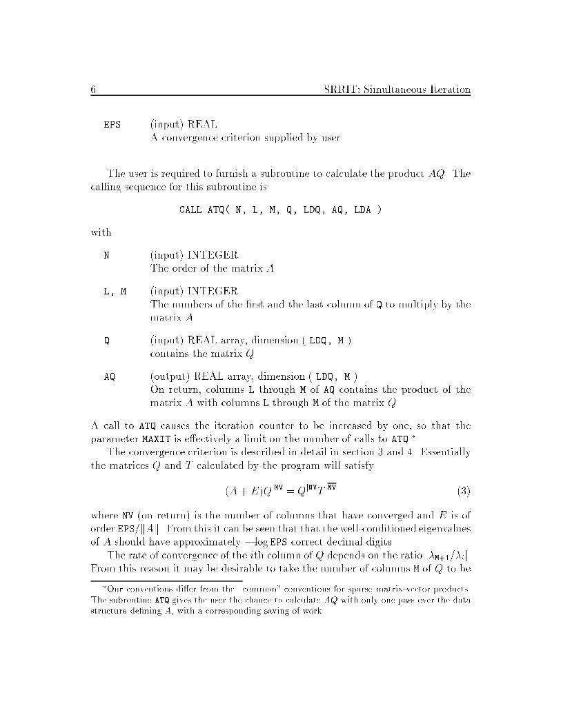
6 SRRIT: Simultaneous IterationEPS (input) REALA convergence criterion supplied by user.The user is required to furnish a subroutine to calculate the product AQ. Thecalling sequence for this subroutine isCALL ATQ( N, L, M, Q, LDQ, AQ, LDA )withN (input) INTEGERThe order of the matrix A.L, M (input) INTEGERThe numbers of the �rst and the last column of Q to multiply by thematrix A.Q (input) REAL array, dimension ( LDQ, M )contains the matrix Q.AQ (output) REAL array, dimension ( LDQ, M )On return, columns L through M of AQ contains the product of thematrix A with columns L through M of the matrix Q.A call to ATQ causes the iteration counter to be increased by one, so that theparameter MAXIT is e�ectively a limit on the number of calls to ATQ.�The convergence criterion is described in detail in section 3 and 4. Essentiallythe matrices Q and T calculated by the program will satisfy(A+ E)QjNV = QjNVT jNV (3)where NV (on return) is the number of columns that have converged and E is oforder EPS=kAk. From this it can be seen that that the well-conditioned eigenvaluesof A should have approximately � log EPS correct decimal digits.The rate of convergence of the ith column of Q depends on the ratio j�M+1=�ij.From this reason it may be desirable to take the number of columns M of Q to be�Our conventions di�er from the \common" conventions for sparse matrix-vector products.The subroutine ATQ gives the user the chance to calculate AQ with only one pass over the datastructure de�ning A, with a corresponding saving of work.

SRRIT: Simultaneous Iteration 7greater than the number of columns NV that one desires to compute. For example,if the eigenvalues A are 1.0, 0.9, 0.5, : : : , it will pay to take M = 2 or 3, even ifonly the eigenvector corresponding to 1.0 is desired.Since SRRIT is designed primarily to calculate the largest eigenvalues of a largematrix, no provisions have been made to handle zero eigenvalues. In particular,zero eigenvalues can cause the program to stop in the auxiliary subroutine ORTH.SRRIT requires a number of auxiliary subroutine (SRRSTP, RESID, GROUP,ORTH, COND) which are described in Section 5. It also requires the LAPACKsubroutines such as SGEHD2, and the some variation of the LAPACK subroutinessuch as SLAQR3 etc. Appendix A contains list of all auxiliary subroutines.SRRIT can be used as a black box. As such the �rst NV vectors it returnswill satisfy (3), although not as many as vectors as the user requests need haveconverged by the time MAXIT is reached. However, the construction of the programhas involved a number of ad hoc decisions. Although the authors have attemptedto make such decisions in a reasonable manner, it is too much to expect that theprogram will perform e�ciently on all distributions of eigenvalues. Consequentlythe program has been written in such a way that it can be easily modi�ed bysomeone who is familiar with its details. The purpose of the next three sectionsis to provide the interested user with these details.3. MethodThe Schur vectors Q of A are computed by a variant of simultaneous iteration,which is a generalization of the power method for �nding the dominant eigen-vector of a matrix. The method has an extensive literature [3, 4, 5, 8, 10], andRutishauser [7] has published a program for symmetricmatrices, from which manyof the features in SRRIT have been drawn. The present variant of simultaneousiteration method has been analyzed in [12].The iteration for computing Q may be described brie y as follows. Start withan n�mmatrixQ0 having orthonormal columns. Given Q�, form Q�+1 accordingto the formula Q�+1 = (AQ�)R�1�+1;where R�+1 is either an identity matrix or an upper triangular matrix chosen tomake the columns of Q�+1 orthonormal (just how often such an orthogonalizationshould be performed will be discussed below). If j�mj > j�m+1j, then under mildrestrictions on Q0 the column space of Q� approaches Qm.

8 SRRIT: Simultaneous IterationThe individual columns of Q� will in general approach the correspondingcolumns of the matrix Q de�ned in Section 1; however the error in the ith columnis proportional to maxfj�i=�i�1j�; j�i+1=�ij�g, and convergence may be intolerablyslow. The process may be accelerated by the occasional application of a \Schur-Rayleigh-Ritz step" (from which SRRIT derives its name), which will now bedescribed. Start with Q� just after an orthogonalization step, so that QT�Q� = I.Form the matrix B� = QT�AQ�;and reduce it to ordered quasi-triangular form T� by an orthogonal similaritytransformation Y�: Y T� B�Y� = T� (4)Finally overwrite Q� with Q�Y�.The matrices Q� formed in this way have the following property. If j�i�1j >j�ij > j�i+1j, then under mild restrictions on Q0 the ith column q(�)i of Q� willconverge approximately linearly to the ith column qi of Q with ratio j�m+1=�ij.Thus not only is the convergence accelerated, but the �rst columns of Q� tend toconverge faster than the later ones.A number of practical questions remain to be answered.1. How should one determine when a column of Q� has converged?2. Can one take advantage of the early convergence of some of the columns ofQ� to save computations?3. How often should one orthogonalize the columns of the Q�?4. How often should one perform the SRR step described above?Here we shall merely outline the answers to these questions. The details will begiven in the next section.1. Convergence. If j�i�1j = j�ij or j�ij = j�i+1j, the ith column of Q is notuniquely determined; and when j�ij is close to j�i+1j or j�i�1j, the ith columncannot be computed accurately. Thus a convergence criterion based on the ithcolumn q(�)i of Q� becoming stationary is likely to fail when A has equimodulareigenvalues. Accordingly we have adopted a di�erent criterion which amounts torequiring that the relation (1) almost be satis�ed. Speci�cally, let t(�)i denote theith column of T� in (4). Then the ith column of the Q� produced by the SRRstep is said to have converged if the 2-norm of the residual vectorr(�)i = Aq(�)i �Qt(�)i (5)

SRRIT: Simultaneous Iteration 9is less than some prescribed tolerance.If this criterion is satis�ed for each column of Q�, then the residual matrixR� = AQ� �Q�T�will be small. This in turn implies that there is a small matrix E� = �R�QT� suchthat (A+ E�)Q� = Q�T�;so that Q� and T� solve the desired eigenproblem for the slightly perturbed matrixA+ E�, provided only that some small eigenvalue of A+ E� has not by happen-stance been included in T�. To avoid this possibility we group nearly equimodulareigenvalues together and require that the average of their absolute values settledown before testing their residuals. In addition a group of columns is tested onlyif the preceding columns have all converged.2. De ation. The theory of the iteration indicates that the initial columnsof the Q� will converge before the later ones. When this happens considerablecomputation can be saved by freezing these columns. This saves multiplying thefrozen columns by A, orthogonalizing them when R�+1 6= I, and work in the SRRstep.3. Orthogonalization. The orthogonalization of the columns of AQ� is a mod-erately expensive procedure, which is to be put o� as long as possible. The dangerin postponing orthogonalization is that cancellation of signi�cant �gures can oc-cur when AQ� is �nally orthogonalized, as it must be just before an SRR step.In [12] it is shown that one can expect no more thant = j log10 �(T ) (6)decimal digits to cancel after j iterations without orthogonalization (here �(T ) =kTk kT�1k is condition number of T with respect to inversion). The relation (6)can be used to determine the number of iterations between orthogonalizations.4. SRR Steps. The SRR step described above does not actually acceleratethe convergence of the Q�; rather it unscramble approximations to the columns ofQm that are already present in the column space of Q� and orders them properly.Therefore, the only time an SRR step needs to be performed is when it is expectedthat a column has converged. Since it is known from the theory of the iterationthat the residual in (5) tends almost linearly to zero, the iteration at which theywill satisfy the convergence criterion can be predicted from their values at twoiterations. As with convergence, this prediction is done in groups correspondingto nearly equimodular eigenvalues.

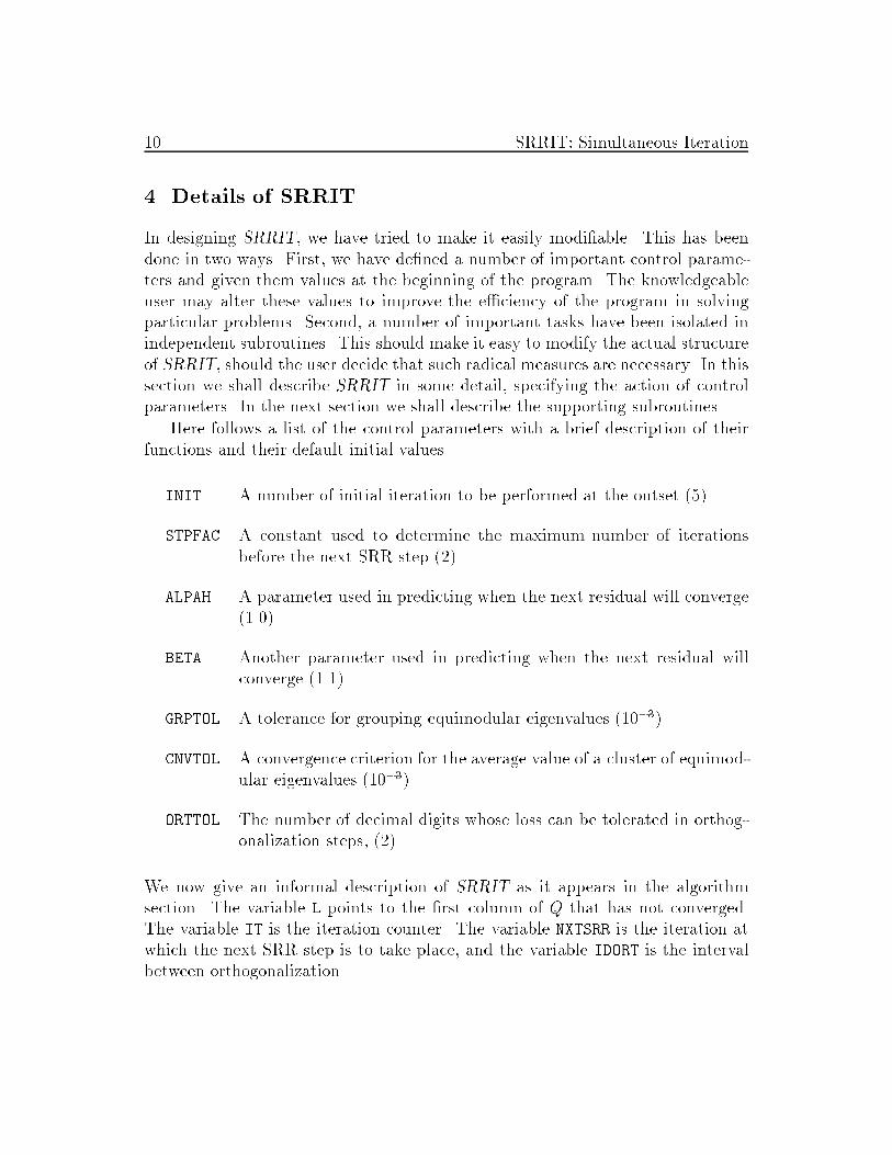
10 SRRIT: Simultaneous Iteration4. Details of SRRITIn designing SRRIT, we have tried to make it easily modi�able. This has beendone in two ways. First, we have de�ned a number of important control parame-ters and given them values at the beginning of the program. The knowledgeableuser may alter these values to improve the e�ciency of the program in solvingparticular problems. Second, a number of important tasks have been isolated inindependent subroutines. This should make it easy to modify the actual structureof SRRIT, should the user decide that such radical measures are necessary. In thissection we shall describe SRRIT in some detail, specifying the action of controlparameters. In the next section we shall describe the supporting subroutines.Here follows a list of the control parameters with a brief description of theirfunctions and their default initial values.INIT A number of initial iteration to be performed at the outset (5).STPFAC A constant used to determine the maximum number of iterationsbefore the next SRR step (2).ALPAH A parameter used in predicting when the next residual will converge(1.0).BETA Another parameter used in predicting when the next residual willconverge (1.1).GRPTOL A tolerance for grouping equimodular eigenvalues (10�3).CNVTOL A convergence criterion for the average value of a cluster of equimod-ular eigenvalues (10�3).ORTTOL The number of decimal digits whose loss can be tolerated in orthog-onalization steps, (2).We now give an informal description of SRRIT as it appears in the algorithmsection. The variable L points to the �rst column of Q that has not converged.The variable IT is the iteration counter. The variable NXTSRR is the iteration atwhich the next SRR step is to take place, and the variable IDORT is the intervalbetween orthogonalization.

SRRIT: Simultaneous Iteration 11SRRIT: 1. initialize control parameters2. initialize1. IT = 0;2. L = 0;3. initialize Q as described by ISTART3. SRR: loop1. perform an SRR step2. compute residuals RSD3. check convergence, resetting L if necessary4. if L > NV or IT � MAXIT then leave SRR5. calculate NXTSRR6. calculate IDORT and NXTORT7. Q = AQ; IT = IT + 18. ORTH: loop until IT = NXTSRR1. POWER: loop until IT = NXTORT1. AQ = AQ2. Q = AQ3. IT = IT+1end POWER2. orthogonalize Q3. NXTORT = min(NXTSRR, IT+IDORT)end ORTHend SRR4. NV = L-1end SRRITThe details of this outline are as follows (the numbers correspond to the state-ments in the algorithm).2.3 If ISTART � 0, then Q is initialized using the random number generationfunction SLARND, then orthonormalized by ORTH. If ISTART = 1, then Q is suppliedby user, and is orthogonalized by calling subroutine ORTH. If ISTART > 1, theinitial orthonomalized Q is supplied by user.3. This is the main loop of the program. Each time an SRR step is performedand convergence is tested.3.1. The SRR step is performed by the subroutine SRRSTP, which returns thenew Q and AQ, as well as T and its eigenvalues.3.2. The residuals RSD are computed by the subroutine RESID.

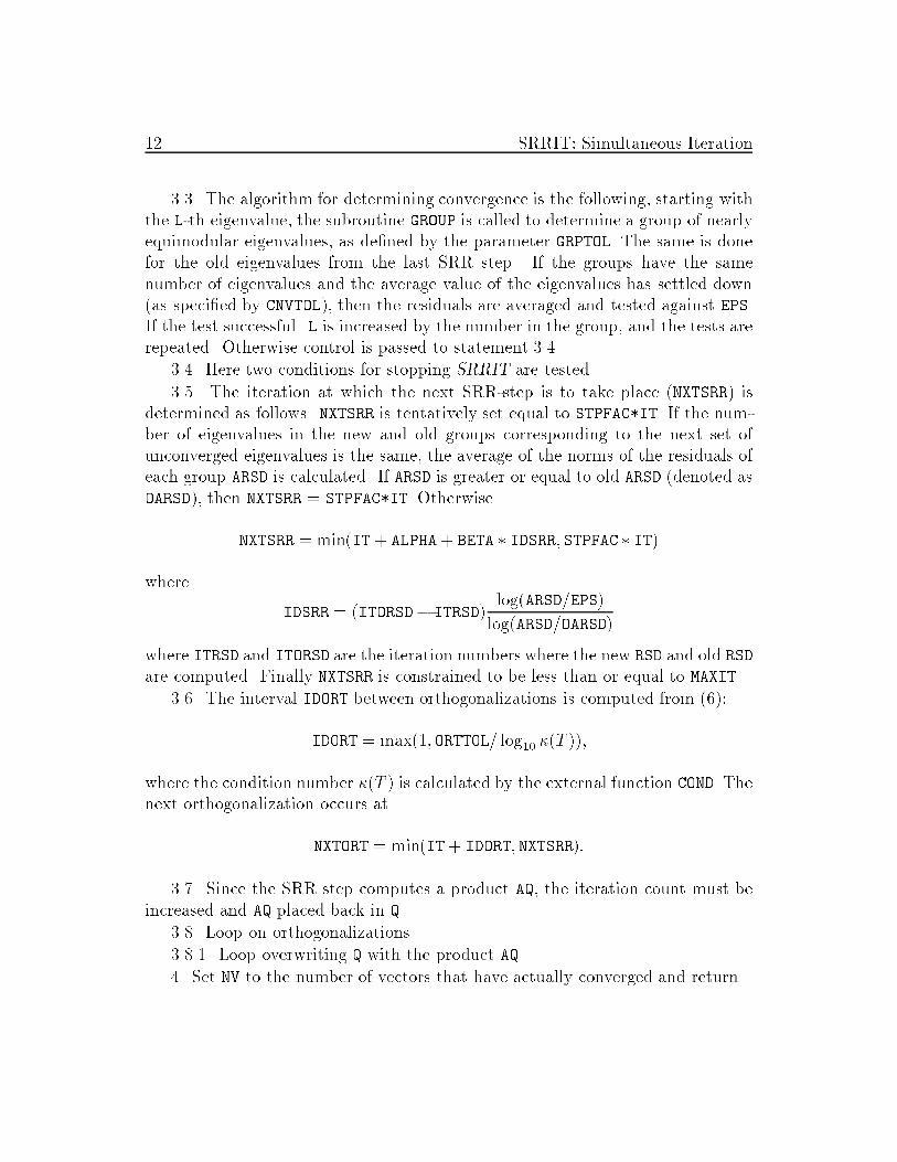
12 SRRIT: Simultaneous Iteration3.3. The algorithm for determining convergence is the following, starting withthe L-th eigenvalue, the subroutine GROUP is called to determine a group of nearlyequimodular eigenvalues, as de�ned by the parameter GRPTOL. The same is donefor the old eigenvalues from the last SRR step. If the groups have the samenumber of eigenvalues and the average value of the eigenvalues has settled down(as speci�ed by CNVTOL), then the residuals are averaged and tested against EPS.If the test successful. L is increased by the number in the group, and the tests arerepeated. Otherwise control is passed to statement 3.4.3.4. Here two conditions for stopping SRRIT are tested.3.5. The iteration at which the next SRR-step is to take place (NXTSRR) isdetermined as follows. NXTSRR is tentatively set equal to STPFAC*IT. If the num-ber of eigenvalues in the new and old groups corresponding to the next set ofunconverged eigenvalues is the same, the average of the norms of the residuals ofeach group ARSD is calculated. If ARSD is greater or equal to old ARSD (denoted asOARSD), then NXTSRR = STPFAC*IT. OtherwiseNXTSRR = min(IT+ ALPHA+ BETA � IDSRR; STPFAC � IT)where IDSRR = (ITORSD� ITRSD) log(ARSD=EPS)log(ARSD=OARSD)where ITRSD and ITORSD are the iteration numbers where the new RSD and old RSDare computed. Finally NXTSRR is constrained to be less than or equal to MAXIT.3.6. The interval IDORT between orthogonalizations is computed from (6):IDORT = max(1; ORTTOL= log10 �(T ));where the condition number �(T ) is calculated by the external function COND. Thenext orthogonalization occurs atNXTORT = min(IT+ IDORT; NXTSRR):3.7. Since the SRR step computes a product AQ, the iteration count must beincreased and AQ placed back in Q.3.8. Loop on orthogonalizations.3.8.1. Loop overwriting Q with the product AQ.4. Set NV to the number of vectors that have actually converged and return.

SRRIT: Simultaneous Iteration 135. Auxiliary SubroutinesIn this section we shall describe some of the subroutines called by SRRIT. All therequired subroutines and their corresponding functionalities are listed in AppendixA. These subroutines have been coded in greater generality than is strictly requiredby SRRIT in order to make the program easily modi�able by the user.SRRSTP( N, L, M, Q, LDQ, AQ, LDA, T, LDT, WR, WI, U, LDU, WORK,LWORK, INFO )This subroutine performs an SRR step on columns L through M of Q. After form-ing AQ and T = QT(AQ), the routine calls BLAS 2 LAPACK routine SGEHD2to reduce T to upper Hessenberg form, then the subroutine SLAQR3 is called toreduce T to ordered quasi-triangular form. The triangularizing transformation Uis postmultiplied into Q and AQ. The new computed eigenvalues are placed in thearrays WR, WI.RESID( N, L, M, Q, LDQ, AQ, LDA, T, LDT, RSD )This subroutine computes the norm of the residuals (5) for columns L throughM of Q. For a complex pair of eigenvalues, the average of the norms of their tworesiduals is returned.GROUP( L, M, WR, WI, RSD, NGRP, CTR, AE, ARSD, GRPTOL )This subroutine locates a group of approximately equimodular eigenvalues �L; �L+1;: : : ; �N+NGRP�1. The eigenvalues so grouped satisfyjj�ij � CTRj � GRPTOL � CTR; i = L; L+ 1; : : : ; L+ NGRP� 1:The mean of the group is returned in AE.ORTH( N, L, M, Q, LDQ, INFO )This subroutine orthonormalizes column L through M of the array Q with respect tocolumn 1 through M. Column 1 through L-1 are assumed to be orthonormalized.The method used is the modi�ed Gram-Schmidtmethod with reorthogonalization.No more than MAXTRY reorthogonalizations are performed (currently, MAXTRY is setto 5), after which the routine executes a stop. The routine will also stop if anycolumn becomes zero.

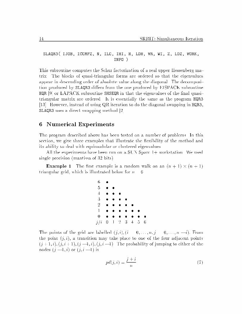
14 SRRIT: Simultaneous IterationSLAQR3( IJOB, ICOMPZ, N, ILO, IHI, H, LDH, WR, WI, Z, LDZ, WORK,INFO )This subroutine computes the Schur factorization of a real upper Hessenberg ma-trix. The blocks of quasi-triangular forms are ordered so that the eigenvaluesappear in descending order of absolute value along the diagonal. The decomposi-tion produced by SLAQR3 di�ers from the one produced by EISPACK subroutineHQR [9] or LAPACK subroutine SHSEQR in that the eigenvalues of the �nal quasi-triangular matrix are ordered. It is essentially the same as the program HQR3[13]. However, instead of using QR iteration to do the diagonal swapping in HQR3,SLAQR3 uses a direct swapping method [2].6. Numerical ExperimentsThe program described above has been tested on a number of problems. In thissection, we give three examples that illustrate the exibility of the method andits ability to deal with equimodular or clustered eigenvalues.All the experiments have been run on a SUN Sparc 1+ workstation. We usedsingle precision (mantissa of 32 bits).Example 1. The �rst example is a random walk on an (n + 1) � (n + 1)triangular grid, which is illustrated below for n = 6.6 �5 � �4 � � �3 � � � �2 � � � � �1 � � � � � �0 � � � � � � �j=i 0 1 2 3 4 5 6The points of the grid are labelled (j; i); (i = 0; : : : ; n; j = 0; : : : ; n � i): Fromthe point (j; i), a transition may take place to one of the four adjacent points(j +1; i); (j; i+1); (j � 1; i); (j; i� 1). The probability of jumping to either of thenodes (j � 1; i) or (j; i� 1) is pd(j; i) = j + in (7)

SRRIT: Simultaneous Iteration 15with the probability being split equally between the two nodes when both nodesare on the grid. The probability of jumping to either of the nodes (j + 1; i) or(j; i+ 1) is pu(j; i) = 1� pd(j; i): (8)with the probability again being split when both nodes are on the grid.If the (n + 1)(n + 2)=2 nodes (j; i) are numbered 1; 2; : : : ; (n+ 1)(n + 2)=2 insome fashion, then the random walk can be expressed as a �nite Markov chainwhose transition matrix A consisting of the probabilities akl of jumping from nodel to node k (A is actually the transpose of the usual transition matrix; see [6]). Tocalculate the ith element of the vector Aq one need only regard the componentsof q as the average number of individuals at the nodes of the grid and use theprobabilities (7) and (8) to calculate how many individuals will be at node i afterthe next transition.We are interested in the steady state probabilities of the chain, which is ordi-narily the appropriately scaled eigenvector corresponding to the eigenvalue unity.However, if we number the diagonals on the grid that are parallel to the hy-potenuse by 0; 1; 2; : : : ; n, then an individual on an even diagonal can only jumpto an odd diagonal, and vice versa. This means that the chain is cyclic with periodtwo, and that A has an eigenvalue of �1 as well as 1.To run the problem on SRRIT, the nodes of the grid were matched with thecomponents of the vector q in the order (0; 0); (1; 0); : : : ; (n; 0); (0; 1); (1; 1); : : : ; (n�1; 1); (0; 2); : : : :. Note that the matrix A is never explicitly used; all computationsare done in terms of the transition probabilities (7) and (8).The problem was run for a 30 � 30 grid which means N = 496. We took M =6, NV = 4, and EPS = 10�5 . The results for each iteration for each iteration inwhich an SRR step was performed are summarized in the following. The variablesWR and WI are the real and imaginary parts of the eigenvalues. RSD is the norm ofthe corresponding residual. CTR is the center of the current convergence cluster.AE is the average value of the eigenvalues in the cluster. ARSD is the average ofthe residuals ARSD. NXTSRR is the number of iterations to the next SRR step andIDORT is the number to the next orthogonalization.IT = 0WR = 0.8225E-01 -0.5044E-01 -0.1708E-02 -0.1708E-02 0.2715E-01 -0.2220E-01WI = 0.0000E+00 0.0000E+00 0.1173E-01 -0.1173E-01 0.0000E+00 0.0000E+00RSD = 0.5798E+00 0.6257E+00 0.8696E+00 0.8696E+00 0.5774E+00 0.5797E+00NGRP = 1CTR = 0.8225E-01

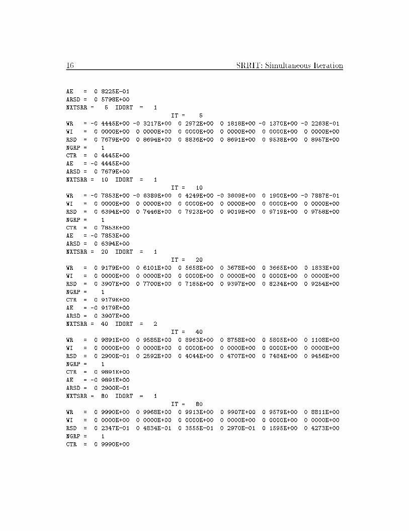
16 SRRIT: Simultaneous IterationAE = 0.8225E-01ARSD = 0.5798E+00NXTSRR = 5 IDORT = 1 IT = 5WR = -0.4445E+00 -0.3217E+00 0.2972E+00 0.1818E+00 -0.1370E+00 -0.2263E-01WI = 0.0000E+00 0.0000E+00 0.0000E+00 0.0000E+00 0.0000E+00 0.0000E+00RSD = 0.7679E+00 0.8694E+00 0.8836E+00 0.8691E+00 0.9538E+00 0.8957E+00NGRP = 1CTR = 0.4445E+00AE = -0.4445E+00ARSD = 0.7679E+00NXTSRR = 10 IDORT = 1 IT = 10WR = -0.7853E+00 -0.6389E+00 0.4249E+00 -0.3609E+00 0.1900E+00 -0.7887E-01WI = 0.0000E+00 0.0000E+00 0.0000E+00 0.0000E+00 0.0000E+00 0.0000E+00RSD = 0.6394E+00 0.7446E+00 0.7923E+00 0.9019E+00 0.9719E+00 0.9758E+00NGRP = 1CTR = 0.7853E+00AE = -0.7853E+00ARSD = 0.6394E+00NXTSRR = 20 IDORT = 1 IT = 20WR = -0.9179E+00 0.6101E+00 -0.5658E+00 0.3678E+00 -0.3665E+00 -0.1833E+00WI = 0.0000E+00 0.0000E+00 0.0000E+00 0.0000E+00 0.0000E+00 0.0000E+00RSD = 0.3907E+00 0.7700E+00 0.7185E+00 0.9397E+00 0.8234E+00 0.9254E+00NGRP = 1CTR = 0.9179E+00AE = -0.9179E+00ARSD = 0.3907E+00NXTSRR = 40 IDORT = 2 IT = 40WR = -0.9891E+00 0.9585E+00 -0.8963E+00 0.8758E+00 -0.5805E+00 0.1108E+00WI = 0.0000E+00 0.0000E+00 0.0000E+00 0.0000E+00 0.0000E+00 0.0000E+00RSD = 0.2900E-01 0.2592E+00 0.4044E+00 0.4707E+00 0.7484E+00 0.9456E+00NGRP = 1CTR = 0.9891E+00AE = -0.9891E+00ARSD = 0.2900E-01NXTSRR = 80 IDORT = 1 IT = 80WR = -0.9990E+00 0.9968E+00 0.9913E+00 -0.9907E+00 -0.9579E+00 0.8811E+00WI = 0.0000E+00 0.0000E+00 0.0000E+00 0.0000E+00 0.0000E+00 0.0000E+00RSD = 0.2347E-01 0.4834E-01 0.3555E-01 0.2970E-01 0.1595E+00 0.4273E+00NGRP = 1CTR = 0.9990E+00

SRRIT: Simultaneous Iteration 17AE = -0.9990E+00ARSD = 0.2347E-01NXTSRR = 160 IDORT = 15 IT = 160WR = -0.1000E+01 0.1000E+01 0.9934E+00 -0.9934E+00 -0.9754E+00 0.9746E+00WI = 0.0000E+00 0.0000E+00 0.0000E+00 0.0000E+00 0.0000E+00 0.0000E+00RSD = 0.5815E-03 0.3167E-02 0.2486E-02 0.6028E-03 0.1128E-01 0.4427E-01NGRP = 2CTR = 0.1000E+01AE = -0.1884E-04ARSD = 0.2277E-02NXTSRR = 320 IDORT = 18 IT = 320WR = -0.1000E+01 0.1000E+01 0.9935E+00 -0.9935E+00 -0.9755E+00 0.9755E+00WI = 0.0000E+00 0.0000E+00 0.0000E+00 0.0000E+00 0.0000E+00 0.0000E+00RSD = 0.3055E-06 0.1198E-05 0.2302E-05 0.5986E-06 0.1712E-03 0.6930E-03NGRP = 2 2 2CTR = 0.1000E+01 0.9935E+00 0.9755E+00AE = -0.2980E-07 0.2980E-06 0.0000E+00ARSD = 0.8745E-06 0.1682E-05 0.5047E-03The course of the iteration is unexceptionable. The program doubles the in-terval between SRR step until it can predict convergence of the �rst cluster cor-responding to the eigenvalues �1. The �rst prediction falls slightly short, but thesecond gets it. The program terminates on the convergence of the second groupof two eigenvalues.To compare the actually costs, runs were made with m = 2; 4; 6; 8, which gavethe following table of iterations and timings (in second) for the convergence of the�rst group of two eigenvalues.m it m� it run time2 1660 3320 49.844 600 2400 37.996 320 1920 32.828 183 1464 27.45As predicted by the convergence theory, the number of iterations decreases as mincreases. However, as m increases we must also multiplymore columns of Q byA,and for this particular problem the number of matrix-vector multiplicationsm�itis probably a better measure of the amount of work involved. From the table itis seen that this measure is also decreasing, although less dramatically than thenumber of iterations. This of course does not include the overhead generated by

18 SRRIT: Simultaneous IterationSRRIT itself, which increases with m and may be considerable. We will see thispoint in the following example 3.Example 2. This example shows how SRRIT can be used in conjunction withthe inverse power method to �nd the smallest eigenvalues of a matrix. Considerthe boundary value problemy00 + �2y = 0;y(0) = 0;y0(0) + y0(1) = 0; 0 < < 1 (9)The eigenvalues of this problem are easily seen to be given by� = i cosh�1(� �1);which are complex. The following table lists the reciprocals of the �rst eighteigenvalues for = 0:01. ��2 j��2j0:012644 � 0:02313i 0:026360:004446 � 0:00739i 0:008540:002895 � 0:00220i 0:003640:001274 � 0:00089i 0:00195 (10)The solution of (9) can be approximated by �nite di�erence techniques as follows.Let yi denote the approximate solution at the point xi = i=(n+1) (i = 0; 1; : : : ; n+1). Replacing the derivatives in (9) with three point di�erence operators, weobtain the following (n+ 1) by (n+ 1) generalized matrix eigenvalue problem fory = (y1; y2; : : : ; yn+1)T: Ay + �2By = 0;where A = 0BBBBBBBBBBBBBBB@ �2 11 �2 11 �2 1. . . . . . . . .. . . . . . . . .1 �2 11 �2 14 �1 �4 3 1CCCCCCCCCCCCCCCA

SRRIT: Simultaneous Iteration 19and B = h2diag(1; 1; : : : ; 1; 0). We may recast this problem in the formCy = 1�2y;where C = A�1B.To apply SRRIT to this problem, we must be able to compute z = Cq for anyvector q. This can be done by solving the linear systemAz = Bq;which is done by sparse Gaussian elimination.The problem was run for n = 300 with M = 6, NV = 4, and EPS = 10�5 . Theresults were the following: IT = 0WR = 0.5990E-02 -0.7362E-03 -0.4792E-03 -0.1994E-03 -0.1419E-03 -0.6238E-04WI = 0.0000E+00 0.0000E+00 0.0000E+00 0.0000E+00 0.0000E+00 0.0000E+00RSD = 0.2616E-01 0.6177E-02 0.4108E-02 0.1956E-01 0.6401E-02 0.9908E-02NGRP = 1CTR = 0.5990E-02AE = 0.5990E-02ARSD = 0.2616E-01NXTSRR = 5 IDORT = 1 IT = 5WR = 0.1264E-01 0.1264E-01 -0.4476E-02 -0.4476E-02 -0.2732E-02 -0.2732E-02WI = 0.2313E-01 -0.2313E-01 0.7324E-02 -0.7324E-02 0.1156E-02 -0.1156E-02RSD = 0.1804E-06 0.1804E-06 0.1965E-04 0.1965E-04 0.8603E-03 0.8603E-03NGRP = 2CTR = 0.2636E-01AE = 0.1264E-01ARSD = 0.1804E-06NXTSRR = 10 IDORT = 1 IT = 10WR = 0.1264E-01 0.1264E-01 -0.4447E-02 -0.4447E-02 -0.2838E-02 -0.2838E-02WI = 0.2312E-01 -0.2312E-01 0.7308E-02 -0.7308E-02 0.2131E-02 -0.2131E-02RSD = 0.2184E-07 0.2184E-07 0.7119E-07 0.7119E-07 0.1584E-03 0.1584E-03NGRP = 2 2 2CTR = 0.2636E-01 0.8555E-02 0.3549E-02AE = 0.1264E-01 -0.4447E-02 -0.2838E-02ARSD = 0.2184E-07 0.7119E-07 0.1584E-03Given the extremely favorable ratios of the eigenvalues in table (10) - theabsolute value of the ratio of the seventh to the �rst is about 0.075, It is not

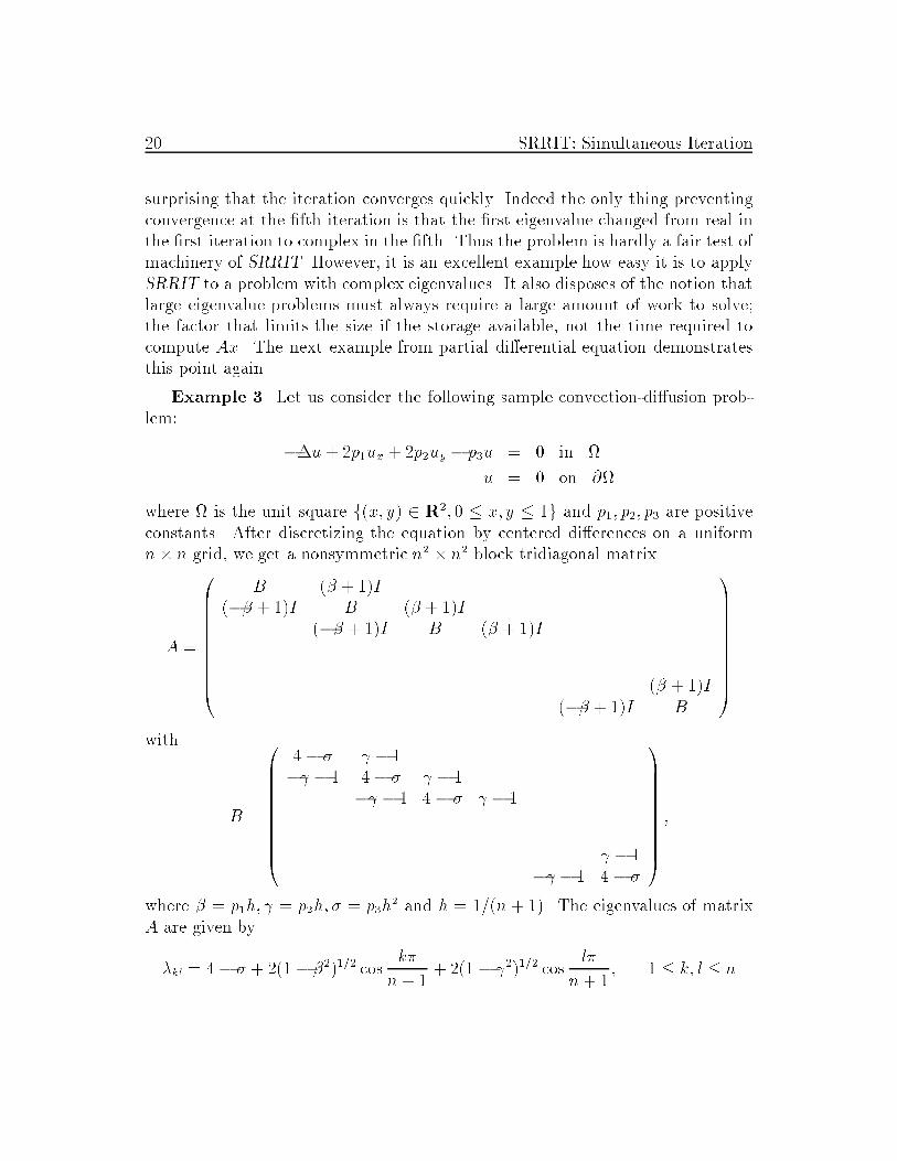
20 SRRIT: Simultaneous Iterationsurprising that the iteration converges quickly. Indeed the only thing preventingconvergence at the �fth iteration is that the �rst eigenvalue changed from real inthe �rst iteration to complex in the �fth. Thus the problem is hardly a fair test ofmachinery of SRRIT. However, it is an excellent example how easy it is to applySRRIT to a problem with complex eigenvalues. It also disposes of the notion thatlarge eigenvalue problems must always require a large amount of work to solve;the factor that limits the size if the storage available, not the time required tocompute Ax. The next example from partial di�erential equation demonstratesthis point again.Example 3. Let us consider the following sample convection-di�usion prob-lem: ��u+ 2p1ux + 2p2uy � p3u = 0 in u = 0 on @where is the unit square f(x; y) 2 R2; 0 � x; y � 1g and p1; p2; p3 are positiveconstants. After discretizing the equation by centered di�erences on a uniformn � n grid, we get a nonsymmetric n2 � n2 block tridiagonal matrixA = 0BBBBBBBBBB@ B (� + 1)I(�� + 1)I B (� + 1)I(�� + 1)I B (� + 1)I. . . . . . . . .. . . . . . (� + 1)I(�� + 1)I B 1CCCCCCCCCCAwith B = 0BBBBBBBBBB@ 4 � � � 1� � 1 4� � � 1� � 1 4 � � � 1. . . . . . . . .. . . . . . � 1� � 1 4 � � 1CCCCCCCCCCA ;where � = p1h; = p2h; � = p3h2 and h = 1=(n + 1). The eigenvalues of matrixA are given by�kl = 4� � + 2(1 � �2)1=2 cos k�n+ 1 + 2(1 � 2)1=2 cos l�n+ 1 ; 1 � k; l � n

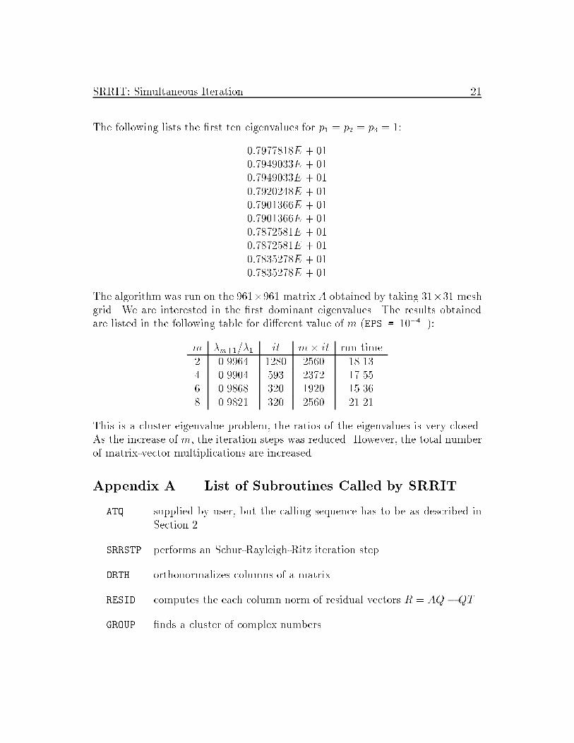
SRRIT: Simultaneous Iteration 21The following lists the �rst ten eigenvalues for p1 = p2 = p3 = 1:0:7977818E + 010:7949033E + 010:7949033E + 010:7920248E + 010:7901366E + 010:7901366E + 010:7872581E + 010:7872581E + 010:7835278E + 010:7835278E + 01The algorithm was run on the 961�961 matrixA obtained by taking 31�31 meshgrid. We are interested in the �rst dominant eigenvalues. The results obtainedare listed in the following table for di�erent value of m (EPS = 10�4 ):m �m+1=�1 it m� it run time2 0.9964 1280 2560 18.134 0.9904 593 2372 17.556 0.9868 320 1920 15.368 0.9821 320 2560 21.21This is a cluster eigenvalue problem, the ratios of the eigenvalues is very closed.As the increase of m, the iteration steps was reduced. However, the total numberof matrix-vector multiplications are increased.Appendix A. List of Subroutines Called by SRRITATQ supplied by user, but the calling sequence has to be as described inSection 2.SRRSTP performs an Schur-Rayleigh-Ritz iteration step.ORTH orthonormalizes columns of a matrix.RESID computes the each column norm of residual vectors R = AQ�QT .GROUP �nds a cluster of complex numbers.

22 SRRIT: Simultaneous IterationSLAQR3 computes the Schur factorization of a real upper Hessenberg matrix,the eigenvalues of Schur form appear in descending order of magni-tude along its diagonal. This subroutine is a variant of LAPACKsubroutine SLAHQR for computing the Schur decomposition.COND estimates the l1-norm condition number with respect to inversion ofan upper Hessenberg matrix.SLARAN generates a random real number from a uniform (0,1) distribution.SORGN2 forms all or part of a real orthogonal matrix Q, which is de�ned as aproduct of k Householder transformations.SLAEQU Standardization of a 2 by 2 blockSubroutins from BLASISAMAX �nds the index of element having max. absolute value.SCOPY copy a vector x to vector y.SDOT inner product of two vectors xTy.SROT applies a plane rotation.SAXPY saxpy operation: �x+ y ! y.SSCAL scale a vector by a constant.SSWAP interchanges two vectors.SNRM2 compute 2-norm of a vector.SGEMV matrix-vector multiplication.SGER performs thr rank 1 updating: �x � yT +A! A.SGEMM matrix-matrix multiplication.

SRRIT: Simultaneous Iteration 23Subroutines from LAPACKSGEHD2 reduces a full matrix to upper Hessenberg matrix (BLAS 2 code).STREXC moves a given 1 by 1 or 2 by 2 diagonal block of a real Schur matrixto the speci�ed position.SLAEXC swaps adjacent diagonal blocks (1 by 1 or 2 by 2) of a Schur matrix.SLARFG generates Householder transformation.SLARF(X)applies Householder transformation.SLASY2 solves up to 2 by 2 Sylvester equation AX �XB = C.SLALN2 solves up to 2 by 2 linear system equation (A� �I)x = b.SLANV2 computes the Schur decomposition of a 2 by 2 matrix.SLADIV computes complex division in real arithmetic.SLAPY2 computes pa2 + b2.SLARTG generates a plane rotation.SLANGE computes norm of a general matrix.SLANHS computes norm of a Hessenberg matrix.SLASSQ called by SLANGE and SLANHS.SLAZRO initializes a matrix.SLACPY copy from one array to another array.SLAMCH determines machine parameters, such as machine precisioni SLABAD.LSAME checks character parameter.XERBLA An error handler routine (return error messages).

24 SRRIT: Simultaneous IterationReferences[1] E. Anderson, Z. Bai, C. Bischof, J. Demmel, J. Dongarra, J. DuCroz, A.Greenbaum, S. Hammarling, A. Mckenney, S. Ostrouchov and D. Sorensen,LAPACK Users' Guide, Release 1.0, SIAM, Philadelphia, 1992.[2] Z. Bai and J. Demmel, On swapping diagonal blocks in real Schur form,submitted to Lin. Alg. Appl. 1992[3] F. L. Bauer, Das Verfahren der Treppeniteration und verwandte Ver-fahren zur Losung algebraischer Eigenwertprobleme, Z. Angew, Math. Phys.8(1957), pp.214-235.[4] M. Clint and A. Jennings, The evaluation of eigenvalues and eigenvectorsof a real symmetric matrix by simultaneous iteration, Comput. J. 13(1970),pp.68-80[5] A. Jennings and W. J. Stewart, A simultaneous iteration method for theunsymmetric eigenvalue problem, J. Inst. Math. Appl. 8(1971), pp.111-121.[6] W. Feller, An introduction to probability theory and its applications, JohnWiley, New York, 1961[7] H. Rutishauser, Computational aspects of F. L. Bauer's simultaneous itera-tion method, Numer. Math. 13(1969), pp.4-13.[8] H. Rutishauser, Simultaneous iteration method for symmetric matrices, Nu-mer. Math. 16(1970), pp.205-223.[9] B. T. Smith, J. M. Boyle, B. S. Garbow, Y. Ikebe, V. C. Klema and C. B.Moler, Matrix eigensystem routines { EISPACK guide, Lec. Notes in Comp.Sci. 6, Springer, New York, 1974[10] G. W. Stewart, Accelerating the orthogonal iteration for the eigenvalues of aHermitian matrix, Numer. Math. 13(1969), pp.362-376.[11] G. W. Stewart, Introduction to Matrix Computations, Academic Press, NewYork, 1973.[12] G. W. Stewart, Simultaneous iteration for computing invariant subspaces ofnon-Hermitian matrices, Numer. Math. 25(1976), pp.123-126.

SRRIT: Simultaneous Iteration 25[13] G. W. Stewart, HQR3 and EXCHNG: FORTRAN subroutines for calculatingthe eigenvalues of a real upper Hessenberg matrix in a prescribed order, ACMTrans. Math. Software 2(1976), pp.275-280.