Electronic copy available at: http://ssrn.com/abstract =1641387 Electronic copy available at: http://ssrn.com/abstract =1641387 HIGH FREQUENCY TRADING AND ITS IMPACT ON MARKET QUALITY Jonathan A. Brogaard ∗ Northwestern University Kellogg School of Management Northwestern University School of Law JD-PhD Candidate [email protected]First Draft: July 16, 2010 November 22, 2010 ∗ I would like to thank my advisors, Thomas Brennan, Robert Korajczyk, Robert McDonald, and Annette Vissing-Jor gensen, for the considerable amount of time they have spent discussing this topic with me; the Zell Center for Risk Research for its financ ial support ; and the many facul ty memb ers and PhD stud ents at the Kellogg School of Mana geme nt, North weste rn Univ ersi ty and at the Northwes tern Unive rsit y School of Law for assis tanc e on this paper . Pleas e contact the author befor e citing this preliminary work.
Transcript
8/6/2019 ssrn-id1641387
http://slidepdf.com/reader/full/ssrn-id1641387 1/70Electronic copy available at: http://ssrn.com/abstract=1641387Electronic copy available at: http://ssrn.com/abstract=1641387
∗I would like to thank my advisors, Thomas Brennan, Robert Korajczyk, Robert McDonald, and Annette Vissing-Jorgensen,
for the considerable amount of time they have spent discussing this topic with me; the Zell Center for Risk Research for its
financial support; and the many faculty members and PhD students at the Kellogg School of Management, Northwestern
University and at the Northwestern University School of Law for assistance on this paper. Please contact the author before
citing this preliminary work.
8/6/2019 ssrn-id1641387
http://slidepdf.com/reader/full/ssrn-id1641387 2/70Electronic copy available at: http://ssrn.com/abstract=1641387Electronic copy available at: http://ssrn.com/abstract=1641387
Abstract
In this paper I examine the impact of high frequency trading (HFT) on the U.S. equities mar-
ket. I analyze a unique dataset to study the strategies utilized by high frequency traders (HFTs), their
profitability, and their relationship with characteristics of the overall market, including liquidity, price
discovery, and volatility. The 26 HFT firms in the dataset participate in 68.5% of the dollar-volume
traded. I find the following key results: (1) HFTs tend to follow a price reversal strategy driven by orderimbalances, (2) HFTs earn gross trading profits of approximately $2.8 billion annually, (3) HFTs do
not seem to systematically engage in a non-HFTr anticipatory trading strategy, (4) HFTs’ strategies are
more correlated with each other than are non-HFTs’, (5) HFTs’ trading levels change only moderately
as volatility increases, (6) HFTs add substantially to the price discovery process, (7) HFTs provide the
best bid and offer quotes for a significant portion of the trading day and do so strategically so as to
avoid informed traders, but provide only one-fourth as much book depth as non-HFTs, and (8) HFTs
may dampen intraday volatility. These findings suggest that HFTs’ activities are not detrimental to
non-HFTs and that HFT tends to improve market quality.
8/6/2019 ssrn-id1641387
http://slidepdf.com/reader/full/ssrn-id1641387 3/70Electronic copy available at: http://ssrn.com/abstract=1641387Electronic copy available at: http://ssrn.com/abstract=1641387
1 Introduction
This paper examines the role of high frequency trading (HFT; HFTs refers to multiple high frequency
traders and HFTr for a single trader) in the U.S. equities market.1 HFT is a type of investment strategy
whereby stocks are rapidly bought and sold by a computer algorithm and held for a very short period,usually seconds or milliseconds.2 The advancement of technology over the last two decades has altered
how markets operate. No longer are equity markets dominated by humans on an exchange floor conducting
trades. Instead, many firms employ computer algorithms that receive electronic data, analyze it, and
publish quotes and initiate trades. Firms that use computers to automate the trading process are referred
to as algorithmic traders; HFTs are the subset of algorithmic traders that most rapidly turn over their stock
positions. Today HFT makes up a significant portion of U.S. equities market activity, yet the academic
analysis of its activity in the financial markets has been limited. This paper aims to start filling the gap.
The rise of HFT introduces several natural questions. The most fundamental is how much market
activity is attributable to HFTs. In my sample 68.5% of the dollar-volume traded involves HFT.3 A second
question that arises is what HFTs are doing. Within this question lie many concerns regarding HFT,
including whether HFTs systematically anticipate and trade in front of non-HFTs, flee in volatile times,
and earn exorbitant profits.4 My findings do not validate these concerns. The third integral question is
how it is impacting asset pricing characteristics. This paper is an initial attempt to answer this difficult
question. The key characteristics I analyze are price discovery, liquidity, and volatility. I find that HFTs
add substantially to the price discovery process, frequently provide inside quotes while providing only
some additional liquidity depth, and may dampen intraday volatility.
Specifically this paper addresses the following eight questions:
High Frequency Traders’ Profitability and Determinants:
1. What determinants influence HFTs’ market activity?
1While this paper examines several important questions regarding HFT, it does not attempt to analyze flash quotes, latency
arbitrage, quote stuffing, or the order book dynamics of HFTs. These are important issues but beyond the scope of this paper.2A more detailed description of HFT is provided in Appendix B.3I estimate that HFTs participate in 77% of the dollar-volume traded in U.S. equities.4“Systematically anticipate and trade in front of non-HFTs” refers to anticipatory trading, whereby HFTs predict when a
non-HFTr is about to buy (sell) a stock and a HFTr takes the same position prior to the non-HFTr. The HFTr then buys (sells) at
a lower (higher) price than the non-HFTr and can turn around and sell (buy) the stock to (from) the non-HFTr at a small profit.
I avoid the term “front running” as it has illegal connotations and is typically used when there is a fiduciary duty between the
involved parties to the above-described activity. As the HFTs in my dataset are identified only as propriety trading firms they
almost certainly have no fiduciary obligation to non-HFTs.
different investment time horizons. Froot, Scharfstein, and Stein (1992) find that short-term speculators
may put too much emphasis on short term information and not enough on stock fundamental information.
The result is a decrease in the informational quality of asset prices. Vives (1995) finds that the market
impact of short term investors depends on how information arrives. The informativeness of asset prices is
impacted differently based on the arrival of information: “with concentrated arrival of information, short
horizons reduce final price informativeness; with diffuse arrival of information, short horizons enhance it”
(Vives, 1995). The theoretical work on short horizon investors suggests that HFT may either benefit or
harm the informational quality of asset prices.
The empirical work relating to HFT either uses indirect proxies for HFT, studies algorithmic trading
(AT), or examines the May 6, 2010 “flash crash.” Regarding work on indirect proxies for HFT, Kearns,
Kulesza, and Nevmyvaka (2010) show that HFTs’ profits in the U.S. equities market have an upper bound
of $21.3 billion from demand-taking trading. They come to this conclusion by analyzing NYSE Trade and
Quote (TAQ) data under the assumption that HFTs initiate trades only when they will be profitable if held
for a pre-determined time period. Hasbrouck and Saar (2010) study millisecond strategies by observing
trading activity around order book adjustments. They find that such low-level activity reduces volatility
and spreads, and increases book depth.
The empirical AT literature finds that AT either has no impact or reduces volatility, increases liquidity,
and adds to the price discovery process.5 Hendershott and Riordan (2009) use data from the Deutsche
Boerse DAX index stocks to examine the information content in AT. In their dataset, ATs supply 50% of
liquidity. They find that AT increases the efficiency of the price process and contributes more to price
discovery than does human trading. Also, they find a positive relationship between ATs providing the
best quotes for stocks and the size of the spread, suggesting that ATs supply liquidity when the payoff is
high and take liquidity when doing so is inexpensive. The study finds little evidence of any relationship
between volatility and AT. Hendershott, Jones, and Menkveld (2010) utilize a dataset of NYSE electronic
message traffic to proxy for algorithmic liquidity supply and study how AT impacts liquidity. The time
period of their analysis surrounds the staggered introduction of autoquoting on NYSE, so they use this
event as an exogenous instrument for AT.6 The study finds that AT increases liquidity and lowers bid-ask
5I am unaware of a study that provides an estimate of the fraction of U.S. equities market activity involving ATs and so I am
unable to determine what fraction of ATs are HFTs.6“Autoquoting” is a technology put in place in 2003 by the NYSE to assist specialists in their role of displaying the best bid
spreads. Chaboud, Hjalmarsson, Vega, and Chiquoine (2009) look at AT in the foreign exchange market.
Like Hendershott and Riordan (2009), they find no causal relationship between AT and volatility. They
find that human order flow is responsible for a larger portion of the return variance, which suggests that
humans contribute more to the price discovery process than do algorithms in currency markets. Gsell
(2008) takes a simple algorithmic trading strategy and simulates the impact it would have on markets if
implemented. He finds that the low latency of algorithmic traders reduces market volatility and that the
large volume of trading increases AT’s impact on market prices.7
Studies on the May 6, 2010 flash crash find that HFTs did not ignite the downfall, but they disagree as
to whether HFTs enhanced the magnitude of the decline. The joint SEC and CFTC (September 30, 2010)
official report describes in detail the events of that day. It finds that HFTs initially provided liquidity to the
large sell order that was identified as the cause of the crash, but that after fundamental buyers withdrew
from the market, HFTs, and all liquidity providers, also stopped trading and providing competitive quotes.
Kirilenko, Kyle, Samadi, and Tuzun (2010) provide additional insight to the activities of different traders
on May 6, 2010 in the E-mini S&P 500 stock index futures market. They conclude that while HFTs did
not ignite the flash crash, their activities enhanced market volatility. Easley, de Prado, and O’Hara (2010)
argue that order flow toxicity, a term referring to a higher likelihood of a trade resulting in a loss, was the
cause of the flash crash. The order flow toxicity signalled days in advance the increased likelihood of a
liquidity-induced crash.
This paper adds to the literature in a variety of ways. It is the first to document the prominence of
HFT in the U.S. equities market. It estimates HFTs’ profits, documents their trading strategy, and tests for
anticipatory trading by HFTs. It also examines HFTs’ order book depth, analyzes which traders supply
liquidity to informed traders, and uses the 2008 short sale ban as a natural experiment to study HFTs’
impact on volatility. Finally, it applies methodologies previously used in the AT literature to study HFTs’
trading strategy correlation and their contribution to price discovery.
and offer. It was implemented under NYSE Rule 60(e) and provides an automatic electronic update, as opposed to a manual
update by a specialist, of customers’ best bid and offer limit orders.7“Latency” in HFT nomenclature refers to the time it takes to receive, process, and respond to market information. Appendix
The data in this paper come from a variety of sources. I use CRSP data when considering daily data
not included in the HFT dataset. Compustat data are used to incorporate stock characteristics in to the
analysis. Trade and Quote (TAQ) data are used to incorporate additional intraday information. Finally, I
use the CBOE S&P 500 Volatility Index (VIX) to capture market-wide volatility.
3.2 High Frequency Trading Data
The unique dataset (the HFT dataset) used in this study contains trades, inside quotes, and the order
book for 120 U.S. stocks, whose symbols, company names, and market capitalization groups are listed in
Table A-1.8 The Trade data contain all trades that occurred on the Nasdaq exchange during regular trading
hours in 2008, 2009, and 02/22/2010 - 02/26/2010, excluding trades that occurred at the opening, closing,
and during intraday crosses.9 The trades are millisecond timestamped and identify what type of trader
(HFTr or non-HFTr) is supplying liquidity and demanding liquidity. By supplying (or providing) liquidity
I mean the limit order standing on the order book that was hit by a marketable order (i.e., a market order or
a more recent limit order taking the opposite side of the transaction and that crossed prices). The liquidity
demander (or taker or initiator) is the market participant who enters the marketable order.
10
The Quotedata are from 02/22/2010 - 02/26/2010 and include the best bid and ask that is being offered at all times
by HFTs and non-HFTs. The Book data are from the first full week of the first month of each quarter in
8The stocks were selected by Terrence Hendershott and Ryan Riordan.9Nasdaq offers opening, closing, and intraday crosses. A cross is a two-step batch order whereby in the first step Nasdaq
accumulates all outstanding orders entered into the cross system and sets a preliminary transaction price. If there is an imbalance
in orders it displays the price to dealers and they can submit orders. Given the final number of orders, the transaction price is
set.10As there are “flash trades” in the data set, let me briefly discuss what they are and how they show up in the data. Flash
quoting is a technology that Nasdaq, BATS, and DirectEdge implemented to facilitate trading on their exchanges. Nasdaq ran
the program from April 2009 to July 2009. A market participant who was going to enter a market order had the option of flashing his quote. For instance, if person A put in a market buy order on Nasdaq and selected for the order to “flash” if not
fillable on Nasdaq and Nasdaq did not have the national best offer, then before Regulation NMS required Nasdaq to send the
order to the exchange with the best offer price, the following events would occur. Person B, likely a HFTr, would be shown the
market order for 20-30 milliseconds and in that time could place an offer matching or bettering the national best offer. If person
B did not provide the offer, the trade would route to the other exchange. If person B did respond to the flashed quote, then
the trade would execute on Nasdaq between persons A and B. In my data this would show up as person A being the liquidity
provider (think of the flashable market order as a 30 millisecond limit order that converts to a market order) and person B would
be the liquidity taker, however, the price the transaction occurred at would be at the offer, even though the liquidity taker was
havior. Market capitalization and market-to-book are used to incorporate established asset pricing infor-
mation of importance; VIX to capture overall market volatility; stock-level volatility to measure stock-
specific price fluctuations; spread, depth, non-HFTr trade size, and non-HFTr dollar-volume traded as
measures of liquidity; autocorrelation to detect whether HFTs are more active in stocks that are more pre-
dictable. Some variables in this regression analysis may be endogenously determined, which can bias the
coefficients. Therefore, I perform the same regression analysis with only the most plausibly exogenous
variables: market capitalization, VIX, and the market-to-book ratio. The analysis is done for all trading
days in the HFT dataset.
Table A-3 reports the results. Columns (1) - (6) show the standardized coefficients, and columns (7)
- (12) show the regular coefficients.14 I perform the regression with the dependent variable capturing the
fraction of shares involving HFT in any capacity (All), as the liquidity taker (Dem.), and as the liquidity
supplier (Sup.).
The results of the full regression analysis show how important and positive is the relationship between
HFTs’ fraction of market activity and market capitalization. The market-to-book variable has a negative
coefficient, suggesting HFTs prefer value stocks. The VIX coefficient implies HFTs increase their demand
for liquidity in volatile markets and decrease their supply. The stock volatility coefficient is only statisti-
cally significant for HFT-demand and it is negative. The spread coefficient is only statistically significant
for the HFT-all regression and is positive. The depth coefficient is negative for HFT-demand and positive
for HFT-supply. The average non-HFTr trade size coefficient is positive for HFT-demand and negative for
HFT-supply. The Non HFT dollar-volume traded is not statistically significant. Finally, the autocorrelation
coefficient is only statistically significant for HFT-supply and is positive. The restricted regression does
not change the sign or statistical significance of any of the included regressors and has minimal impact on
the magnitude of their coefficients.
14Standardized coefficients are calculated by running an OLS regression analysis after all the variables have been demeanedand have been scaled by their standard deviations. The standardized coefficients’ interpretation is that a one standard deviation
change in an independent variable is expected to change the dependent variable by β standard deviations. The regressors
underlying scale of units are irrelevant due to the pre-regression scaling. Thus, the larger the standardized coefficient, the larger
the impact that variable has on the dependent variable.
where 1Sell is a dummy indicator equal to one if HFTs sold a stock in transaction t and zero otherwise,
1Buy is similarly defined for HFTs buying, Pricet is the price at which transaction t occurred, Sharest is
the number of shares exchanged in transaction t. The second term in the equation corrects for the end-
of-day inventory balance. Summing up the Profit for each stock on a given day results in the total HFT
profitability for that day. The result is that on average HFTs make $298,000 per day from their Nasdaq
trades in these 120 stocks. Figure 2 displays the time series of HFT profitability per day. The graph is a
five-day moving average of HFTs’ daily profitability for the 120 stocks in the HFT dataset. Profitability
varies substantially over time, even after smoothing out the day-to-day fluctuations.21 HFTs’ profitability
per dollar traded is $.000072.22 I estimate HFTs Sharpe ratio assuming HFTs require capital to be able to
fund the maximum inventory imbalance that occurs in any one hour period. In the HFT dataset this means
HFTs require $117 million in capital ($4.68 billion when considering the entire U.S. equities market).
This implies HFTs have an annualized Sharpe ratio of 4.5 before expenses.
I extrapolate from the within-sample estimate of profitability to the entire U.S. equities market. To do
so, I estimate the fraction of shares involving HFTs using the exogenous regression coefficient estimates
20This assumption is consistent with conversations I have had with HFTs who say they avoid holding positions overnight. In
addition, it is consistent with HFTs balancing their inventory throughout the day so as never to accumulate a large long or short
position, which can be observed in the HFT dataset from the fact that HFTs typically switch between being long and short in a
stock several times a day.21The most profitable day in the figure is September 29, 2008. On this day the House of Representatives failed to pass the
initial TARP bill. The least profitable day is January 23, 2009. I am unaware of any significant event occurring on this date.22I calculate this by taking the average daily profit of HFTs from trades in the HFT dataset and divide it by the average daily
where Market Cap is the log of the daily shares outstanding of stock i multiplied by the closing price
of stock i, Market/Book is the ratio of stock i’s market value divided by the Compustat book value based
on the most recent preceding quarterly report, Winsorized at the 99th percentile, and VIX is the S&P 500
Chicago Board of Exchange Volatility Index. HFT is calculated for each stock on each day. I multiply
HFT by the dollar-volume traded for each stock on each day in 2008 and 2009, and I multiply this value by
the profit per dollar traded of $.000072 estimated in the in-sample analysis. I am assuming that the profit
per dollar traded is the same across stocks. I divide the total sum by two as the data covers a two-year
period:
HFT Annual Profit =1
2
N i=1
T t=1
HFTi,t ∗ DVolumei,t ∗ 0.000072
(2)
The result of this calculation is that HFTs gross profit is approximately $ 2.8 billion annually on trading
of $39.3 trillion ($50.4 trillion when including HFT-to-HFT trades, which implies they are involved in 77%
of all U.S. equities dollar-volume traded).25
No adjustment is made for transaction costs yet. Such costs will be relatively small as HFTs pay to
trade only when they take liquidity and they receive a rebate when they provide liquidity. For example,
Nasdaq offers $.20 per 100 shares to high-volume liquidity providers. On the other hand, Nasdaq charges
$.25 per 100 shares to traders who take liquidity. I use the fraction of shares where HFTs take liquidity and
23As the regression analysis conducted in Table A-3 is not bound between 0 and 1 I set a lower limit of 0% and an upper
limit of 95% of HFTs’ fraction of market participation.
24The fraction of dollar-volume HFTs are not trading with each other is 0.780, which I obtain by calculating the dollar-volumewhere HFTs are on only one side of a trade divided by the total dollar-volume in which HFTs are involved: (DVolumeHN +DVolumeNH )/(DVolumeHH +DVolumeHN +DVolumeNH ). As I am trying to determine the profitability of the HFT industry,
when I multiply the average profit per dollar traded I only consider the dollars traded with non-HFTs, as a trade between two
HFTs has a net zero profit for the industry.25This number is less than what others have estimated. An article by the Tabb Group claimed HFTs made around $21 billion
annually. However, the $2.8 billion annually from U.S. equities is in line with other claims. For instance, a Wall Street Journal
article states that Getco made around $400 million in 2008 across all of its divisions (it trades on fifty exchanges around the
world and in equities, commodities, fixed income, and foreign exchange. Even if Getco, one of the largest HFT firms, earned
$150 million of that profit from U.S. equities it would still be in line with my findings.
provide liquidity from Table 1 Panel A to estimate the explicit Nasdaq trading costs. Using the average
stock price in 2008 and 2009 of $37.10 and the finding that HFTs take liquidity in 50.98% of the dollar-
volume they trade and provide it in 49.02%, I estimate HFTs annual net exchange transaction costs to be
$399.6 million.
Besides knowing how profitable HFTs are, it is also informative to know how profitable they are com-
pared to traditional market makers. Hasbrouck and Sofianos (1993) and Coughenour and Harris (2004)
study the trading activity and profitability of the NYSE specialists. In the HFT dataset HFTs earn less
than 1/100th of a penny ($0.000072) per dollar traded. Using the reported summary data in Coughenour
and Harris (2004), specialists in 2000 (after decimalization, before decimalization reported in parentheses)
made $0.00052 ($0.000894) per dollar traded in small stocks, $0.00036 ($0.00292) per dollar traded in
medium stocks, and $.00059 ($.0025) per dollar traded in large stocks.26
From this perspective, HFTs are
almost one-seventh as expensive as traditional market makers.27 Part of this earning discrepancy could
be that HFTs and traditional market makers are being compensated for different kinds of risks. Whereas
HFTs tend to close the day in a neutral position, traditional market markets often hold inventory for days
or weeks.
5.4 Testing Whether High Frequency Traders Systematically Engage in Anticipatory Trading
In this section I test whether HFTs systematically anticipate and trade in front of non-HFTs (“anticipatory
trading”) (SEC, January 14, 2010). It may be that HFTs predict and buy (sell) a stock just prior to when a
non-HFTr buys (sells) the stock. If this is the case, HFTs are profiting at the expense of non-HFTs. 28
To determine whether HFTs are implementing an anticipatory trading strategy, I analyze the frequency
26I calculate the gross profits in Coughenour and Harris (2004) by applying the following formula:
Profit Per Dollar TradedStock Size = Specialists Gross ProfitsTable 5/(PriceTable 1 Panel A ∗ Total Shares TradedTable 1 Panel C ∗Specialist Share Participation RatesTable 2 Panel A).
27I do not make adjustments for inflation.28Anticipatory trading is not itself an illegal activity. It is illegal when a firm has a fiduciary obligation to its client and uses
the client’s information to front run its orders. In my analysis, as HFTs are propriety trading firms, they do not have clients andso the anticipatory trading they may be conducting would likely not be illegal. Where HFT and anticipatory trading may be
problematic is if market manipulation is occurring that is used to detect orders. It may be the case that “detecting” orders would
fall in to the same category of behavior as that resulted in a $2.3 million fine to Trillium Brokerage Services for “layering”.
Trillium was fined for the following layering strategy: Suppose Trillium wanted to buy stock X at $20.10 but the current offer
price was $20.13, Trillium would put in a hidden buy order at $20.10 and then place several limit orders to sell where the limit
orders were sufficiently below the bid price to be executed. Market participants would see this new influx of sell orders, update
their priors, and lower their bid and offer prices. Once the offer price went to $20.10, Trillium’s hidden order would execute and
Trillium would then withdraw its sell limit orders. FINRA found this violated NASD Rules 2110, 2120, 3310, and IM-3310
(now FINRA 2010, FINRA 2020, FINRA 5210, and also part of FINRA 5210).
algorithmic trading, while others, such as Barclay, Hendershott, and McCormick (2003), use the technique
to compare information from different markets.31 I calculate the impulse response function on a trade-by-
trade basis using 10 lags for trades by HFTs and non-HFTs. I estimate the impulse response function
for each stock for each day. As in Barclay, Hendershott, and McCormick (2003) and Hendershott and
Riordan (2009), I estimate three equations, a midpoint quote return equation, a HFTr trade equation, and
a non-HFTr trade equation. The 10-lag vector auto regression (VAR) is:
rt =10i=1
αirt−i +10i=0
βiqH t−i +
10i=0
γ iqN t−i + ϵ1,t, (7)
qH t =10i=1
δirt−i +10i=0
ρiqH t−i +
10i=0
ζ iqN t−i + ϵ2,t, (8)
qN t =10
i=1 πirt−i +10
i=0 ν iqH t−i +
10
i=0 ψiqN t−i + ϵ3,t. (9)
where t is a trade-event based time indicator, i indicates the number of lagged events, qH is a signed
indicator for HFTr trades taken a value of +1 for a HFTr initiated buy, -1 for HFTr initiated sell, and 0
otherwise, qN is a similarly designated indicator for non-HFTr trades, rt is the quote midpoint to quote
midpoint return between trade changes, and the Greek letters are the coefficients for the different regres-
sors.
After estimating the VAR, I invert it to get the vector moving average (VMA) model to obtain: rt
qH t
qN t
=
a(L) b(L) c(L)
d(L) e(L) f (L)g(L) h(L) i(L)
ϵ1,t
ϵ2,tϵ3,t
, (10)
where the vectors a(L) - i(L) are lag operators. Hasbrouck (1991a) interprets the impulse response
function for HFT,∑10
t=0 b(L), as the private information content of an innovation in HFT. The non-HFT
impulse response function is∑10
t=0 c(L) and is the private information content of an innovation in non-
HFT.32 The expected portion of a trade should not impact prices and so should not show up in the impulse
response function; however, the unexpected portion, the innovation, of a trade should influence the price
of future trades. The impulse response function estimates this impact on future trades. By examining a
31The HFT dataset is especially well suited for this as it is in milliseconds and thus minimizes the problem of multiple trades
occurring within one time period, as occurs with data denoted in seconds.32The impulse response function is a technology first used in the macro-economic literature to determine the impact of an
exogenous shock to the economy as it worked its way through the economy. Hasbrouck (1991a) and Hasbrouck (1991b) took
this methodology and applied it to the microstructure literature.
only to non-HFTs’ limit orders. In Table 6 Panel B I report the price impact difference in basis points and
dollars. The results suggest HFTs provide more liquidity in large stocks than in small. The price impact is
monotonically increasing and almost linear within each stock size category.
In Table 6 Panel C the results are reported for the same analysis but with consideration to an elimination
of non-HFTs’ limit orders. The price impact is substantially more than in Panel B across all stock size
categories and for all trade sizes. These results suggest that, while HFTs provide some liquidity depth, it
is only a fraction of that provided by non-HFTs.
A concern with this analysis is the endogeneity of limit orders (Rosu, 2009) and the information
they may contain (Harris and Panchapagesan, 2005; Cao, Hansch, and Wang, 2009). That is, a market
participant who sees a limit order at a given price or in a certain quantity (or absence thereof) may alter
his behavior as a result. The analysis I do is only for a partial equilibrium setting and does not attempt to
incorporate general equilibrium dynamics into the results. Also, the most important part of this table is the
comparison between HFTr and non-HFTr book depth. It is not clear whether, once a market participant
observed a given limit order, he would place his own limit order, place a marketable order, or withdraw
from the market. In a general equilibrium setting it is not a priori clear whether the price impact would be
larger or smaller than the results in Table 6.37
Next, I show how order book depth by different traders varies over time. While Table 6 presents
the average price impact in different settings, Figure 4 depicts the time series price impact a 1000-share
trade would have if it were to hit the order book. There are three graphs: the total price impact the trade
would have with all available liquidity accessible, the price impact difference from removing HFTs’ limit
orders, and the price impact difference from removing non-HFTs’ limit orders. The order book data is
available only during 10 5-day windows. The X-axis identifies the first day in the 5-day window.38 There
is considerable variation over time in the overall depth of the order book and the amount provided by HFTs
and non-HFTs. Even so, HFTs on average provide strictly less liquidity than do non-HFTs on each day. 39
37In addition, this concern should be further dampened as market participants can always choose not to display their limit
orders.38That is, the observation 01-07-08 is followed by observations on January 8th, 9th, 10th, and 11th of 2008. The next
observation is for April 7, 2008 and is followed by the next four consecutive trading days.39The correlation coefficient between the VIX and the non-HFTs / HFTs book ratio is -.38, thus when expected volatility is
high, the difference between HFTs and non-HFTs book depth narrows.
on average provide more liquidity to informed traders. Twenty stocks have nHFT being greater than HFT
and the difference being statistically significant, while none have a statistically significant difference in
the other direction. The results suggest that HFTs are more selective than non-HFTs in how they supply
liquidity, especially in large stocks, and this culminates in their not matching the best bid or offer when
they suspect they will be trading with informed traders.
6.3 High Frequency Trading’s Impact on Volatility
The final market quality measure I analyze is the causal relationship between HFT and volatility. I have
already considered volatility in previous areas, both the general relationship and also the impact of an
exogenous shock to volatility on HFTs’ market participation. In this section I examine whether HFT
impacts volatility. I implement two methodologies to examine the question. First, I do an event study
around the September 2008 short-sale ban. Second, I compare the price paths of stocks with and without
HFTs being part of the data generation process in a partial equilibrium setting. Both methodologies suggest
HFT tends to dampen volatility.
6.3.1 A Natural Experiment Around the Short-Sale Ban
In this section I utilize an exogenous shock to HFTs’ activity to study the impact HFT has on volatility.
The exogenous shock I study is the September 19, 2008 ban on short selling on 799 financial stocks.40 Of
the 120 stocks in the HFT dataset, 13 were on the ban list.
The ban indirectly stopped some HFTs from trading in the banned stocks. While the ban did not
explicitly require HFT firms to stop trading the affected stocks, it did undermine their trading strategy. The
strategies used by HFTs require them to be able to freely switch between being long or short a stock.41 To
verify that the short sale was a de facto ban on HFT, I graph the time series activity of HFTs’ fraction of
market involvement in Figure A-1.42 The figure shows that HFTs’ activity dropped precipitously for the
13 affected stocks during the ban. One reason HFT did not drop to zero for the affected stocks is that a
portion of HFT firms were designated market makers and not subject to the short-sale ban restrictions. 43
40The ban was in place until October 9, 2008.41I cannot observe this in the data, but have been told by HFT firms that this is the case.42The fraction of the market is normalized so that HFTs’ fraction of trading in the affected and unaffected stocks are equal
on September 1, 2010.43The initial announcement of the short-sale ban provided a limited exemption for option market makers, but on September
22, 2008 the SEC extended the option market maker exemption to sell short the 799 affected stocks.
J. Hasbrouck and G. Saar. Low-latency trading. NYU Working Paper , 2010.
J. Hasbrouck and G. Sofianos. The trades of market makers: An empirical analysis of NYSE specialists.
Journal of Finance, 48(5):1565–1593, 1993.
J.A. Hausman, A.W. Lo, and A.C. MacKinlay. An ordered probit analysis of transaction stock prices.
Journal of Financial Economics, 31(3):319–379, 1992.
T. Hendershott and P.C. Moulton. Speed and stock market quality: The NYSE’s Hybrid. UC Berkeley
Working Paper , 2010.
T. Hendershott and R. Riordan. Algorithmic trading and information. UC Berkeley Working Paper , 2009.
T. Hendershott, C.M. Jones, and A.J. Menkveld. Does algorithmic trading improve liquidity? Journal of
Finance, Forthcoming, 2010.
M. Kearns, A. Kulesza, and Y. Nevmyvaka. Empirical limitations on high frequency trading profitability.
Univ. of Pennsylvania Working Paper , 2010.
A.A. Kirilenko, A.S. Kyle, M. Samadi, and T. Tuzun. The flash crash: The impact of high frequencytrading on an electronic market. CFTC Working Paper , 2010.
I. Rosu. A dynamic model of the limit order book. Review of Financial Studies, 22(11):4601–4641, 2009.
SEC. Concept release on equity market structure. January 14, 2010.
SEC and CFTC. Findings regarding the market events of may 6, 2010. September 30, 2010.
M. Van der Wel, A. Menkveld, and A. Sarkar. Are market makers liquidity suppliers? VU Univ. Working
paper , 2008.
X. Vives. Short-term investment and the informational efficiency of the market. Review of FinancialStudies, 8(1):125–160, 1995.
Figure 3: High Frequency Traders’ Participation as Day-Level Volatility Changes. This figure depicts how
HFTs’ participation varies as day-level volatility changes. The X-axis represents 100 bins grouped together based
on the V-Level value: V-Leveli,t =V i,t−E (V i)
E (V i)∗ 1σi
, where V i,t is the 15-minute realized volatility for stock i on day
t, and σi is the standard deviation of stock i’s V . The V-Level variable is the scaled deviation from the mean, where
it is scaled by the standard deviation of a stock’s volatility, σi. The Y-axis is the percent change from HFTs’ average
trading activity, HFT-Level j =∑
V-Leveli,tϵj1N j
HFTi,t−E (HFTi)
E (HFTi)
where HF T is the fraction of shares in which
HFTs are involved and j is the V-Level bin stock i at time t is falls into. N is the number of observations in bin j.There are three graphs, HFT and Volatiltiy - All, which looks at all HFTs activity, HFT and Volatility - Liquidity
Supply, which only considers HFTs’ supplying liquidity activity, and HFT and Volatility - Liquidity Demand, which
only considers HFTs’ demanding liquidity activity. In each graph there are four lines. The bin-by-bin HFT-Level, a
nine-bin centered moving average of the HFT-Level, and the upper and lower 95 % confidence intervals.
Figure 4: Time Series of High Frequency Traders’ and Non High Frequency Traders’ Book Depth. This
Figure analyzes the depth of the order book and how much depth different types of traders provide by analyzing the
price impact of a 1000 share trade hitting the order book with and without different types of traders. There are three
graphs. The first, Price Impact of a 1000 Share Trade, examines the total price impact a 1000 share trade would
have with all available liquidity accessible. The second graph, Additional Price Impact without HFTs on the Book,
depicts the additional price impact that would occur from removing HFTs’ limit orders The third graph, Additional
Price Impact without non-HFTs on the Book, graphs the additional price impact from removing non-HFTs’ limit
orders. The daily dollar price impact value is calculated giving equal weight to each stock. The order book data isavailable during 10 5-day windows. The X-axis identifies the first day in the 5-day window. That is, The observation
01-07-08 is followed by observations on January 8th, 9th, 10th, and 11th of 2008. The next observation is for April 7,
2008 and is followed by the next four consecutive trading days. To separate the 5-day windows I enter a zero-impact
trade, creating the evenly spaced troughs.
0
. 2
. 4
. 6
$ P r i c e
I m p a c t
1 − 7 −
0 8
4 − 7 −
0 8
7 − 7 −
0 8
9 − 1 5
− 0 8
1 0 − 6
− 0 8
1 − 5 −
0 9
4 − 1 3
− 0 9
7 − 6 −
0 9
1 0 − 5
− 0 9
2 − 2 2
− 1 0
Date
Price Impact of a 1000 Share Trade
0
. 1
. 2
. 3 $ P r i c e I m p a c t
1 − 7 −
0 8
4 − 7 −
0 8
7 − 7 −
0 8
9 − 1 5
− 0 8
1 0 − 6
− 0 8
1 − 5 −
0 9
4 − 1 3
− 0 9
7 − 6 −
0 9
1 0 − 5
− 0 9
2 − 2 2
− 1 0
Date
Additional Price Impact without HFTs on the Book
0
. 2
. 4
. 6
. 8
1
$ P r i c e I m p a c t
1 − 7 −
0 8
4 − 7 −
0 8
7 − 7 −
0 8
9 − 1 5
− 0 8
1 0 − 6
− 0 8
1 − 5 −
0 9
4 − 1 3
− 0 9
7 − 6 −
0 9
1 0 − 5
− 0 9
2 − 2 2
− 1 0
Date
Additional Price Impact without non−HFTs on the Book
Table 1: High Frequency Trading’s Fraction of Trade Activity. This table reports the aggregate day-level fraction
of trading involving HFTs for all trades in the HFT dataset. Panel A measures the fraction of dollar-volume in which
HFTs are involved , Panel B measures the fraction of trades involving HFTs, and Panel C measures the fraction
of shares traded involving HFTs. Within each panel are three categories. The first category, HFT-All, reports the
fraction of activity where HFTs are either demanding liquidity, supplying liquidity, or doing both. The second
category, HFT-Demand, reports the fraction of activity where HFTs are demanding liquidity. The third category,
HFT-Supply, shows the fraction of activity where HFTs are supplying liquidity. Within each category I report the
findings by stock size, with each bin having 40 stocks and the row Overall reporting the unconditional results. Thereported summary statistics include the mean, standard deviation, minimum, 5th percentile, 25th percentile, median,
75th percentile, 95th percentile, and maximum fraction of activity involving HFTs.
Table 2: High Frequency Trading’s Fraction of the Inside Quote Activity. This table reports the summary statistics based
on HFTs best bid and offer activity in each stock on each day. Panels A - F report the percent of the time HFTs offer the
same or better bid or offer as non-HFTs. Panel G reports the fraction of quote changing activity arising from HFTs. Panels A
- C measure time based on calendar time; Panels D - F measure time based on tick time, weighting each observation equally
regardless of the calendar time of the quote. Panels A and D report the unconditional percent of time HFTs are at the best bid
or offer. I divide the observations into days on which the bid - ask spread is lower and higher than average for each stock.
I report the conditional percent of time for days where the spread is lower than average in Panels B and E, and higher than
average in Panels C and F. Within each category I report the findings by stock size, with each bin having 40 stocks and the row
Total reporting the unconditional results. The reported summary statistics include the mean, standard deviation, minimum, 5thpercentile, 25th percentile, median, 75th percentile, 95th percentile, and maximum. For Panels A - F the column “% of Inside”
reports the average percent of the total shares HFTs provide at the inside quotes, conditional on HFTs being at the inside quotes.
The data are from 02/22/2010 - 02/26/2010.
Panel A: All
Stock Size Mean Std. Dev. % Of Inside Min. 5% 25% 50% 75% 95% Max.
Table 3: 10-Second High Frequency Trading Determinants: Order Imbalance and Lagged Returns. This table reports
the results from performing the logit regression: HFTi,t = α+Reti,1−10∗β1−10+OIBi,1−10∗β11−20+OIBi,1−10∗Reti,1−10∗β21−30 + ϵi,t, HFTi,s takes on one of six definitions: (1) HFTs buying, (2) HFTs buying and supplying liquidity, (3) HFTs
buying and demanding liquidity, (4) HFTs selling, (5) HFTs selling and supplying liquidity, and (6) HFTs selling and demanding
liquidity. The dependent variable equals one if, on net, HFTs are engaging in that activity and zero otherwise. The explanatory
variables include Reti,1−10, the return for stock i in period s, where s is the number of 10-second time periods prior to the time
t, OIBi,1−10, a dummy variable derived from the order imbalance that equals 1 if OIB i,s =Buy Initiated Sharesi,s−Sell Initiated Sharesi,s
Shares Outstandingi,s
is ≤ 0 for the Buy regressions, and ≥ 0 for the Sell regressions. Each explanatory variable is followed by a subscript between1 and 10 that represents the number of lagged time periods away from the event occurring in the time t dependent variable. I
perform the regression on all stocks from 02/22/2010 - 02/26/2010. Stock fixed effects are implemented and standard errors
are clustered by stock. The table reports the results for the marginal effects at the means for the probability of the dependent
variable equaling one for stock i at time t.
(1) (2) (3) (4) (5) (6)
Buy - ALL Buy - Supply Buy - Demand Sell - ALL Sell - Supply Sell - Demand
T a b l e 5 : T h e P e r m a n e n t P r i c e I m p a c t o f T r a d e s b y H i g h F r e q
u e n c y T r a d e r s a n d N o n H i g h F r e
q u e n c y T r a d e r s . T h i s t a b l e r e p o r t s r e s u l t s f r o m d i f f e r e n t
p e r m a n e n t p r i c e i m p a c t m e a s
u r e s c a l c u l a t e d f o r e a c h s t o c k o n e a c h d a y . P a n e l A r e p o r t s t h e a v e r
a g e l o n g - r u n ( 1 0 e v e n t s i n t h e f u t u r e ) i m p u l s e r e s p o n s e
f u n c t i o n f o r H F T r - a n d n o n - H
F T r - i n i t i a t e d t r a d e s . T h e i n t e r p r e t a t i o n i s t h a t t h e l a r g e r a t r a d e r ’ s i m p u l s e r e s p o n s e f u n c t i o n t h e m o r e p r i v a t e i n f o r m a t i o n f r o m
t h a t t r a d e r ’ s t r a d e s . P a n e l B r e p o r t s t h e a v e r a g e l o n g - r u n - s h o r t - r u n ( 1 0 e v e n t s i n t h e f u t u r e - t h e
c o n t e m p o r a n e o u s e v e n t ) i m p u l s e
r e s p o n s e f u n c t i o n f o r
H F T s a n d n o n - H F T s . A l a r g e r l o n g r u n - s h o r t r u n i m p u l s e r e s p o n s e d i f f e r e n c e s u g g e s t s t h e i n f o r m a
t i o n i n t h e i n i t i a l t r a d e t a k e s t i m e t o b e i m p u t e d , w h e r e a s
a n e g a t i v e d i f f e r e n c e s u g g e s t s
t h e r e i s a n i m m e d i a t e o v e r r e a c t i o n
t o t h e t r a d e ’ s i n f o r m a t i o n . P a n e l C
r e p o r t s t h e a v e r a g e l o n g - r u n i m p u l s e r e s p o n s e f u n c t i o n
f o r H F T r - a n d n o n - H F T r - s u p p
l i e d t r a d e s . A l a r g e r v a l u e s u g g e s t s t h a t t r a d e r - t y p e p r o v i d e s m o r e l i q
u i d i t y t o i n f o r m e d t r a d e r s . I n P a n e
l A a n d B I d e fi n e q H
a n d q N
b a s e d o n w h o i s d e m a n d i n g l i q u i d i t y . I n P a n e l C I d e fi n e
t h e q b a s e d o n t h e l i q u i d i t y s u p p l i e
r ’ s a c t i v i t y a n d t r a d e r t y p e . I d e fi n e
q H
t o b e a + 1 w h e n a
H F T r l i q u i d i t y s u p p l i e r s e l l s a
n d - 1 w h e n a H F T r l i q u i d i t y s u p p l i e r b u y s , T h e q N
v a l u e i s s i m i l a r l y d e fi n e d f o r n o n - H F T r s u p p l i e d t r a d e s . E a c h p a n e l r e p o r t s
t h e a v e r a g e p e r c e n t o f d a y s w h e n H F T s ’ p r i c e i m p a c t i s g r e a t e r t h
a n n o n - H F T s ’ . T h e t a b l e a l s o r e p o r t s t h e n u m b e r o f s t o c k s f o r w h i c h t h e d i f f e r e n c e b e t w e e n
H F T a n d n o n - H F T i s s t a t i s t i c
a l l y s i g n i fi c a n t . I n e a c h p a n e l I g r o u p t h e r e s u l t s i n t o t h r e e g r o u p s b
a s e d o n s t o c k m a r k e t c a p i t a l i z a t i o
n , a n d a l s o r e p o r t t h e
o v e r a l l r e s u l t s . I p e r f o r m t h i s
a n a l y s i s f o r 0 2 / 2 2 / 2 0 1 0 - 0 2 / 2 6 / 2 0 1 0 . I c a l c u l a t e s t a t i s t i c a l s i g n i fi c a n c e i n c o r p o r a t i n g N e w e y - W e s t s t a n
d a r d e r r o r s t o c o r r e c t
f o r t h e t i m e - s e r i e s c o r r e l a t i o n
i n o b s e r v a t i o n s .
P a n e l A : L o n g - R u n I m p u l s e R e s p o n s e F u n c t i o n s
S t o c k S i z e
H F T
S t d . D e v .
H F T
n o n - H F T
S t d . D e v . H F T
M e a n %
D a y s H F T > n o n - H F T
S t a t . S i g n H F T < n o n - H F T
S t a t .
S i g n H F T > n o n - H F T
S m a l l
3 . 6 0
1 8 . 0 6
1 . 0 8
9 . 3 1
6 4
3
0
M e d i u m
2 . 3 1
2 . 8 1
1 . 2 0
1 . 9 1
7 4 . 2 1
1
1 2
L a r g e
1 . 0 7
0 . 4 1
0 . 8 1
0 . 4 1
7 8 . 4 6
0
2 1
O v e r a l l
2 . 1 5
9 . 1 4
1 . 0 2
4 . 7 5
7 3 . 3 3
4
3 3
P a n e l B : L o n g - R u n - S h o r t - R
u n I m p u l s e R e s p o n s e F u n c t i o n s
S t o c k S i z e
H F T
S t d . D e v .
H F T
n o n - H F T
S t d . D e v . H F T
M e a n %
D a y s H F T > n o n - H F T
S t a t . S i g n H F T < n o n - H F T
S t a t .
S i g n H F T > n o n - H F T
S m a l l
1 . 2 5
9 . 9 8
- 0 . 7 7
8 . 6 9
0 . 6 1
0
1
M e d i u m
0 . 8 1
2 . 4 9
0 . 3 3
1 . 7 5
0 . 6 4
1
1 4
L a r g e
0 . 5 4
0 . 3 6
0 . 3 6
0 . 3 2
0 . 8 1
0
3 7
O v e r a l l
0 . 8 1
5 . 1 7
0 . 0 7
4 . 4 5
0 . 7 0
1
5 2
T h e S u p p l y o f L i q u i d i t y t o I n
f o r m e d T r a d e r s : T h e P e r m a n e n t P r
i c e I m p a c t o f T r a d e s b a s e d o n w h o S u p p l i e s L i q u i d i t y .
Table 6: High Frequency Traders and Non High Frequency Traders Book Depth. This table reports the partial
equilibrium price impact resulting from different sized market buy orders hitting the book with and without different
liquidity providers. Panel A reports the average price impact different size trades would have given the displayed
and hidden liquidity on the HFT dataset book snapshots. Panel B and C look at the additional price impact in partial
equilibrium that an average trade of varying sizes would have if certain liquidity providers did not have orders on
the order book. Panel B considers the additional price impact that would occur if there were no HFTs on the order
book. Panel C considers the impact if no non-HFTs were on the book. I provide the analysis for stock sizes from
100 - 1000 in increasing trade size increments. I Winsorize the upper tail of the price impact values at the 99.5%level. I report both the basis point price impact and also the dollar size price impact. I divide the results into three
even groups based on stock size and also report the overall results. I find similar results for market sell orders that
are not reported.
Panel A: Price Impact of Trade - All Orders Available
Figure A-1: High Frequency Trading’s Fraction of the Market around the Short-Sale Ban. The figure
shows how HFTs’ fraction of dollar-volume trading varied surrounding the September 19, 2008 SEC
imposed short-sale ban on many financial stocks. In the HFT dataset, 13 stocks are in the ban. The two
graphs plot HFTs’ fraction of dollar-volume traded for the banned stocks and for the unaffected stocks.
The first graph reports the fraction of dollar-volume where HFTs supplied liquidity. The second reportsthe fraction where HFTs demanded liquidity. I normalize the banned stocks’ percent of the market in both
graphs so that the affected and unaffected stocks have the same percent of the market on September 2,
2008. The two vertical lines represent the first and last day of the short-sale ban.
m a g n i t u d e p r i c e i n c r e a s e s . T h e X - a x i s r e p r e s e n t s 1 0 0 b i n s b a s e
d o n t h e R e t - L e v e l v a l u e : R e t - L e v e l i , t , m
=
R e t i , t , m
σ i
, w h e r e R e t i , t , m i s t h e m a x i m u m r e t u r n
f o r s t o c k i o n d a y t d u r i n g p e r i o d m . T h a t i s , R e t i s c a l c u l a t e d
b a s e d o n t h e m a x i m u m a n d m i n i m u m p r i c e d u r i n g a 1 5 - m i n u t e p e r i o d . I f t h e m i n i m u m
p r i c e o c c u r r e d p r i o r t o t h e m a
x i m u m p r i c e i t i s c o n s i d e r e d a p o s i t i v e r e t u r n p e r i o d . T h e h i g h e r t h e p e r c e n t i l e , t h e l a r g e r t h e p r i c e i n c r e
a s e . T h e Y - a x i s i s t h e
p e r c e n t c h a n g e f r o m H F T s ’ a v e r a g e t r a d i n g a c t i v i t y , H F T - L e v e l j =
∑ R e t - L e v e l i , t , m ϵ j
1 N j
[ H F T i , t , m − E
( H F T i )
E ( H F T i )
] , w h e r e H F T t a k e s o n fi v e
d e fi n i t i o n s , w h i c h a r e
t h e g r a p h s ’ l a b e l s : A l l , L i q u i d i t y D e m a n d - B u y , L i q u i d i t y S u p p l y - B u y , L i q u i d i t y D e m a n d - S e l l , a
n d L i q u i d i t y S u p p l y - S e l l . T h e d e fi
n i t i o n o f H F T r e f e r s
t o t h e f r a c t i o n o f d o l l a r - v o l u m
e t r a d e d t h a t s a t i s fi e s t h e s p e c i fi e d
t r a d i n g c r i t e r i a : w h e r e t h e B u y / S e l l r e f e r s t o H F T s ’ a c t i o n , a n d L i q u i d i t y S u p p l y / L i q u i d i t y
D e m a n d r e f e r s t o t h e i r l i q u i d i t y r o l e i n t h e t r a n s a c t i o n . I r e m o v e o b s e r v a t i o n s w h e r e t h e r e t u r n w a s 0 f o r t h a t p e r i o d o r w h e r e l e s s t h a n 3 0 t r a d e s o c c u r r e d . I n
e a c h g r a p h t h e r e a r e f o u r l i n e s . T h e b i n - b y - b i n H F T - L e v e l , a fi v e - b i n c e n t e r e d m o v i n g a v e r a g e o f t h e H F T - L e v e l , a n d t h e u p p e r a n d l o w e r 9 5 % c o n fi d e n c e
i n t e r v a l s .
− . 1 5 − . 1 − . 0 5 0 . 0 5 P e r c e n t C h a n g e f r o m H F T s ’ A v e r a g e T r a d i n g
0
2 0
4 0
6 0
8 0
1 0 0
P r i c e R i s e P e r c e n t i l e
H F T % M
A ( 5 )
H F T %
S E_
h i g h_
s u p p l y
S S E_
l o w_
s u p p l y
L i q u i d i t y S u p p l y −
S e l l
− . 0 6 − . 0 4 − . 0 2 0 . 0 2 . 0 4 P e r c e n t C h a n g e f r o m H F T s ’ A v e r a g e T r a d i n g
0
2 0
4 0
6 0
8 0
1 0 0
P r i c e
R i s e
P e r c e n t i l e
H
F T %
M A ( 5 )
H F T %
S
S E
_ h i g h
_ d e m a n
d
S S E
_ l o w
_ d e m a n
d
L i q u
i d i t y D e m a n
d −
S e
l l
− . 1 − . 0 5 0 . 0 5 P e r c e n t C h a n g e f r o m H F T s ’ A v e r a g e T r a d i n g
0
2 0
4 0
6 0
8 0
1 0 0
P r i c e R i s e P e r c e n t i l e
H F T % M
A ( 5 )
H F T %
S S E_
h i g h_
s u p p l y
S S E_
l o w_ s u
p p l y
L i q u i d i t y S u p p l y −
B u y
− . 1 − . 0 5 0 . 0 5 P e r c e n t C h a n g e f r o m H F T s ’ A v e r a g e T r a d i n g
0
2 0
4 0
6 0
8 0
1 0 0
P r i c e
R i s e
P e r c e n t i l e
H
F T %
M A ( 5 )
H F T %
S
S E
_ h i g h
_ d e m a n
d
S S E
_ l o w
_ d e m a n
d
L i q u
i d i t y D e m a n
d −
B u y
− . 0 6 − . 0 4 − . 0 2 0 . 0 2 P e r c e n t C h a n g e f r o m H F T s ’ A v e r a g e T r a d i n g
h e X - a x i s r e p r e s e n t s 1 0 0 b i n s b a s e
d o n t h e R e t - L e v e l v a l u e : R e t - L e v
e l i , t , m
=
R e t i , t , m
σ i
, w h e r e R e t i , t , m i s t h e m a x i m u m r e t u r n
f o r s t o c k i o n d a y t d u r i n g p e r i o d m . T h a t i s , R e t i s c a l c u l a t e d
b a s e d o n t h e m a x i m u m a n d m i n i m u m p r i c e d u r i n g a 1 5 - m i n u t e p e r i o d . I f t h e m i n i m u m
p r i c e o c c u r r e d a f t e r t h e m a x i m u m p r i c e i t i s c o n s i d e r e d a n e g a t i v e r e t u r n p e r i o d . T h e h i g h e r t h e p e r c e n t i l e , t h e l a r g e r t h e p r i c e d e c r e a s e . T h e Y - a x i s i s t h e
p e r c e n t c h a n g e f r o m H F T s ’ a v e r a g e t r a d i n g a c t i v i t y , H F T - L e v e l j =
∑ R e t - L e v e l i , t , m ϵ j
1 N j
[ H F T i , t , m − E
( H F T i )
E ( H F T i )
] , w h e r e H F T t a k e s o n fi v e
d e fi n i t i o n s , w h i c h a r e
t h e g r a p h s ’ l a b e l s : A l l , L i q u i d i t y D e m a n d - B u y , L i q u i d i t y S u p p l y - B u y , L i q u i d i t y D e m a n d - S e l l , a
n d L i q u i d i t y S u p p l y - S e l l . T h e d e fi
n i t i o n o f H F T r e f e r s
t o t h e f r a c t i o n o f d o l l a r - v o l u m
e t r a d e d t h a t s a t i s fi e s t h e s p e c i fi e d
t r a d i n g c r i t e r i a : w h e r e t h e B u y / S e l l r e f e r s t o H F T s ’ a c t i o n , a n d L i q u i d i t y S u p p l y / L i q u i d i t y
D e m a n d r e f e r s t o t h e i r l i q u i d i t y r o l e i n t h e t r a n s a c t i o n . I r e m o v e o b s e r v a t i o n s w h e r e t h e r e t u r n w a s 0 f o r t h a t p e r i o d o r w h e r e l e s s t h a n 3 0 t r a d e s o c c u r r e d . I n
e a c h g r a p h t h e r e a r e f o u r l i n e s . T h e b i n - b y - b i n H F T - L e v e l , a fi v e - b i n c e n t e r e d m o v i n g a v e r a g e o f t h e H F T - L e v e l , a n d t h e u p p e r a n d l o w e r 9 5 % c o n fi d e n c e
i n t e r v a l s .
− . 0 6 − . 0 4 − . 0 2 0 . 0 2 . 0 4 P e r c e n t C h a n g e f r o m H F T s ’ A v e r a g e T r a d i n g
0
2 0
4 0
6 0
8 0
1 0 0
P r i c e D r o p P e r c e n t i l e
H F T % M
A ( 5 )
H F T %
S S E_
h i g h_
s u p p l y
S S E_
l o w_ s u
p p l y
L i q u i d i t y S u p p l y −
S e l l
− . 0 6 − . 0 4 − . 0 2 0 . 0 2 P e r c e n t C h a n g e f r o m H F T s ’ A v e r a g e T r a d i n g
0
2 0
4 0
6 0
8 0
1 0 0
P r i c e D r o p P e r c e n t i l e
H
F T % M
A ( 5 )
H F T %
S
S E_
h i g h_
d e m a n d
S S E_
l o w_
d e m a n d
L i q u i d i t y D e m a n d − S e l l
− . 1 − . 0 5 0 . 0 5 . 1 P e r c e n t C h a n g e f r o m H F T s ’ A v e r a g e T r a d i n g
0
2 0
4 0
6 0
8 0
1 0 0
P r i c e D r o p P e r c e n t i l e
H F T % M
A ( 5 )
H F T %
S S E_
h i g h_
s u p p l y
S S E_
l o w_ s u
p p l y
L i q u i d i t y S u p p l y −
B u y
− . 1 − . 0 5 0 . 0 5 P e r c e n t C h a n g e f r o m H F T s ’ A v e r a g e T r a d i n g
0
2 0
4 0
6 0
8 0
1 0 0
P r i c e
D r o p
P e r c e n t i l e
H
F T %
M A ( 5 )
H F T %
S
S E
_ h i g h
_ d e m a n
d
S S E
_ l o w
_ d e m a n
d
L i q u
i d i t y D e m a n
d −
B u y
− . 0 3 − . 0 2 − . 0 1 0 . 0 1 P e r c e n t C h a n g e f r o m H F T s ’ A v e r a g e T r a d i n g
p u s t a t s t o c k s i n c l u d e d i n t h e c o m p a r i s o n c o n s i s t o f a l l s t o c k s w i t h d a t a a v a i l a b l e a n d t h a t a r e l i s t e d o n e i t
h e r N a s d a q o r N Y S E ,
w h i c h i n c l u d e s 4 , 2 3 8 s t o c k s .
T h e t a b l e r e p o r t s m a r k e t c a p i t a l i z a t i o n , m a r k e t - t o - b o o k r a t i o , i n d u s t r y , a n d l i s t i n g e x c h a n g e s u m m a r y s t a t i s t i c s a n d p r o v i d e s
t h e t - s t a t i s t i c f o r t h e d i f f e r e n c
e s i n m e a n s . T h e C o m p u s t a t a n d t h e H F T d a t a s e t d a t a a r e f o r s t o c k s 2 0 0 9 e n d - o f - y e a r r e p o r t . I f a s t o c k ’ s y e a r - e n d w a s n o t
1 2 / 3 1 / 2 0 0 9 , I u s e t h e m o s t r e c e n t p r e c e d i n g a n n u a l fi g u r e s . T h e i n d u s t r i e s a r e c a t e g o r i z e d b a s e d o n
t h e F a m a - F r e n c h t e n i n d u s t r y g r o u
p s . P a n e l B c o m p a r e s
t h e m a r k e t c h a r a c t e r i s t i c s o f t h e H F T d a t a s e t t o s t o c k s i n t h e T A
Q d a t a b a s e t h a t a r e l i s t e d o n N Y S E o r N a s d a q a n d h a v e t h e r e q u i s i t e
d a t a , w h i c h r e s u l t s i n
4 , 0 4 5 s t o c k s . I l o o k a t e a c h s t o c k ’ s m a r k e t c h a r a c t e r i s t i c s f o r t h e fi v e t r a d i n g d a y s 0 2 / 2 2 / 2 0 1 0 - 0 2 / 2 6 / 2 0 1 0 . F o r e a c h d a t a s e t I r e p o r t
t h e h a l f s p r e a d , s t o c k
p r i c e , b i d s i z e , o f f e r s i z e , d a i l y v o l u m e t r a d e d , n u m b e r o f t r a d e s , a n d s i z e o f a t r a d e . F o r e a c h v a r i a b l e I r e p o r t t h e t - s t a t i s t i c f o r t h e
d i f f e r e n c e s i n m e a n s
b e t w e e n t h e t w o d a t a s e t s .
P a n e l A : H F T D a t a b a s e
v . C o m p u s t a t D a t a b a s e H
F T D a t a b a s e
C o m p u s t a t D a t a b a s e
M e a n
S t d . D e v .
M i n
.
M e d i a n
M a x .
M e a n
S t d . D e v .
M i n .
M e d i a n
M a x .
T - T e s t
M a r k e t C a p . ( m i l l i o n s )
1 7 5 8 8 . 2 4
3 7 8 5 2 . 3 8
8 0 . 6 0 2 5
1 7 4 3
1 9 7 0 1 2 . 3
3 3 6
7
1 3 8 8 1
. 0 2 2 9
4 0 3 . 3
3 2 2 3 3 4
1 0 . 2 0 6 3
M a r k e t - t o - B o o k
2 . 6 5 0
3 . 1 3 4
- 1 1 . 7 7
9 9
1 . 8 3 7
2 0 . 0 4 0 6
1 3 . 8 1
6 9 0 . 8
- 6 8 8 . 5
1 . 4 5 2
4 4 8 4 4
- 0 . 1 7 7 0
I n d u s t r y - N o n - D u r a b l e s
. 0 3 3 3
. 1 8 0 2
. 0 4 3
8 9
. 2 0 4 9
- 0 . 5 5 8 3
I n d u s t r y - D u r a b l e s
. 0 2 5
. 1 5 6 7
. 0 1 9
8 2
. 1 3 9 4
0 . 3 9 9 9
I n d u s t r y - M a n u f a c t u r i n g
. 1 6 6 6
. 3 7 4 2
. 0 9 2
9 7
. 2 9 0 4
2 . 7 1 6 9
I n d u s t r y - E n e r g y
. 0 0 8 3
. 0 9 1 2
. 0 4 5
7 8
. 2 0 9
- 1 . 9 5 6 8
I n d u s t r y - H i g h T e c h
. 1 5 8 3
. 3 6 6 5
. 1 8 2 4
. 3 8 6 2
- 0 . 6 7 4 0
I n d u s t r y - T e l e c o m .
. 0 5
. 2 1 8 8
. 0 2 7
3 7
. 1 6 3 2
1 . 4 8 1 9
I n d u s t r y - W h o l e s a l e
. 0 9 1 6
. 2 8 9 7
. 0 8 3
7 7
. 2 7 7 1
0 . 3 0 7 6
I n d u s t r y - H e a l t h C a r e
. 1 5
. 3 5 8 5
. 1 0 8 1
. 3 1 0 5
1 . 4 5 2 2
I n d u s t r y - U t i l i t i e s
. 0 3 3 3
. 1 8 0 2
. 0 2 8
5 5
. 1 6 6 6
0 . 3 0 9 4
I n d u s t r y - O t h e r
. 2 8 3 3
. 4 5 2 5
. 3 7 0 2
. 4 8 2 9
- 1 . 9 4 6 9
E x c h a n g e - N Y S E
. 5
. 5 0 2 0
. 3 9 0 5
. 4 8 7 9
2 . 4 2 2 1
E x c h a n g e - N a s d a q
. 5
. 5 0 2 0
. 6 0 9 5
. 4 8 7 9
- 2 . 4 2 2 1
O b s e r v a t i o n s
1 2 0
4 2 3
8
P a n e l B : H F T D a t a b a s e
v . T A Q D a t a b a s e
H F T D a t a b a s e
T A Q D a t a b a s e
V a r i a b l e
M e a n
S t d . D e v .
M i n .
M e d i a n
M a x
.
M e a n
S t d . D e v .
M i n .
M e d i a n
M a x .
T - T e s t
Q u o t e d H a l f S p r e a d ( D o l l a r s )
. 0 7 1 1
. 0 8 6 3
. 0 0 5 7
. 0 4 7 9
. 7 6 7 5
. 1 3 4 9
. 2 0 1 6
. 0 0 5
. 0 7 1 4 2
2 . 7 8 6
- 7 . 6 9 9
S t o c k P r i c e ( D o l l a r s )
3 5 . 4 2
4 0
. 0 2
4 . 6 2 3
2 6 . 4 6
3 4 7 . 4
2 6 . 1 1
3 0 . 9 6
5 . 0 1
1 8 . 9 0
7 0 5 . 9 5
1 1 . 7 2
B i d S i z e ( H u n d r e d s o f S h a r e s )
2 3 . 8 8
6 8
. 6 9
1 . 2 1 6
3 . 6 1 5
9 8 9 . 3
1 5 . 5 5
2 3 1 . 1
1
3 . 4 7
1 8 7 7 0
0 . 8 7 7
O f f e r S i z e ( H u n d r e d s o f S
h a r e s )
2 4 . 2 4
7 0
. 6 9
1 . 1 1 5
3 . 8 5 7
8 8 2 . 6
1 4 . 3 1
1 8 6 . 8
1
3 . 6 4 2
1 0 4 4 1
1 . 2 9 4
D a i l y V o l u m e T r a d e d ( M i l l i o n s o f D o l l a r s )
T a b l e A - 3 : D a y - L e v e l D e t e r m i n a n t s o f H i g h F r e q u e n c y T r a d i n g ’ s F r a c t i o n o f T r a d e A c t i v i t y
. T h i s t a b l e s h o w s t h e r e s u l t o f a n
O L S r e g r e s s i o n w i t h
o b s e r v a t i o n s a t t h e s t o c k a n d d a y l e v e l . I i m p l e m e n t t h e r e g r e s s i o
n : H i , t =
α +
M C i ∗ β 1
+
M B t ∗
β 2
+
V I X i ∗ β 3
+
σ i , t ∗ β 4
+
S P i , t ∗ β 5
+
D E P i , t ∗ β 6
+
T S i , t ∗ β 7
+
N V i , t ∗ β 8
+
A C i
, t ∗ β 9
+
ϵ i , t , w h e r e H i , t i s t h e f r a c t i o n o f s h a r e s t r a d e d i n v o l v i n g a H F T r i n s t o c k i o n d a y t , M C i s t h e l o g
m a r k e t c a p i t a l i z a t i o n
a s o f D e c e m b e r 3 1 , 2 0 0 9 , M B
i s t h e m a r k e t t o b o o k r a t i o a s o f D
e c e m b e r 3 1 , 2 0 0 9 , w h i c h i s W i n s o r i z e d a t t h e 9 9 t h p e r c e n t i l e , V I X i s
t h e S & P 5 0 0 C h i c a g o
B o a r d o f E x c h a n g e V o l a t i l i t y
I n d e x ( s c a l e d b y 1 0 − 3 ) , σ i s t h e t e n - s e c o n d r e a l i z e d v o l a t i l i t y s u m m
e d u p o v e r t h e d a y ( s c a l e d b y 1 0 − 5 ) , S P i s t h e a v e r a g e
t i m e - w e i g h t e d d o l l a r s p r e a d b e t w e e n t h e b i d a n d o f f e r ( s c a l e d b y
1 0 − 1 ) , D E P i s t h e a v e r a g e t i m e - w e
i g h t e d d e p t h a v a i l a b l e a t t h e i n s i d e
b i d a n d a s k i n d o l l a r s
( s c a l e d b y 1 0 − 3 ) , T S i s t h e a v e r a g e d o l l a r - v o l u m e s i z e o f a n o n - H
F T r - o n l y t r a d e ( t r a d e s w h e r e n o n - H
F T s b o t h s u p p l i e d l i q u i d i t y a n d d e
m a n d e d i t ) ( s c a l e d b y
1 0 − 5 ) , N V i s t h e d o l l a r - v o l u m
e o f n o n - H F T r - o n l y t r a n s a c t i o n s , n o r m a l i z e d b y m a r k e t c a p i t a l i z a t i o n
( a n d s c a l e d b y 1 0 − 6 ) , a n d A C i s t h e a b s o l u t e v a l u e o f a
o n e - p e r i o d a u t o r e g r e s s i v e p r o c e s s ( A R ( 1 ) ) a n a l y z e d a t t e n - s e c o n d i n t e r v a l s ( s c a l e d b y 1 0 − 2 ) . S t a n d a r d e r r o r s a r e c l u s t e r e d b y s t o c k . C o l u m n s 1 - 6 s h o w t h e
s t a n d a r d i z e d b e t a c o e f fi c i e n t s
a n d c o l u m n s 7 - 1 2 d i s p l a y t h e r e g u l a r c o e f fi c i e n t s . T h e d e p e n d e n t v a r i a b l e s f o r t h e c o l u m n a r e : t h e p e r c e
n t o f s h a r e s H F T s a r e
i n v o l v e d i n f o r 1 , 4 , 7 , a n d 1 0 ; t h e p e r c e n t o f s h a r e s i n w h i c h H F T
s d e m a n d l i q u i d i t y f o r 2 , 5 , 8 , a n d
1 1 ; t h e p e r c e n t o f s h a r e s i n w h i c h H F T s s u p p l y l i q u i d i t y
f o r 3 , 6 , 9 , a n d 1 2 . C o l u m n s 4
- 6 a n d 1 0 - 1 2 s h o w t h e r e s u l t s f o r t h e r e s t r i c t e d r e g r e s s i o n a n a l y s i s .
S t a n d a r d i z e d B e t a C
o e f fi c i e n t s
O L S C o e f fi c i e n t s
A l l
D e m .
S u p .
A l l
D e m .
S u p .
A
l l
D e m .
S u p .
A l l
D e m .
S u p .
( 1 )
( 2 )
( 3 )
( 4 )
( 5 )
( 6 )
( 7
)
( 8 )
( 9 )
( 1 0 )
( 1 1 )
( 1 2 )
M a r k e t C a p . ( M C )
0 . 7 9 1 ∗ ∗ ∗
0 . 5 5 8 ∗ ∗ ∗
0 . 7 7 3 ∗ ∗ ∗
0 . 7 6 8 ∗ ∗ ∗
0 . 5 2 9 ∗ ∗ ∗
0 . 7 7 2 ∗ ∗ ∗
0 . 0 8 2 ∗ ∗ ∗
0 . 0 4 3 ∗ ∗ ∗
0 . 0 6 6 ∗ ∗ ∗
0 . 0 8 0
∗ ∗ ∗
0 . 0 4 1 ∗ ∗ ∗
0 . 0 6 6 ∗ ∗ ∗
( 0 . 0 0 5 0 )
( 0 . 0 0 5 0 )
( 0 . 0 0 4 1 )
( 0 . 0 0
3 8 )
( 0 . 0 0 4 3 )
( 0 . 0 0 4 0 )
M a r k e t / B o o k ( M B )
- 0
. 1 2 9 ∗ ∗
- 0 . 0 8 8
- 0 . 1 2 4 ∗ ∗ ∗
- 0 . 1 3 9 ∗ ∗
- 0 . 0 4 3
- 0 . 1 9 3 ∗ ∗ ∗
- 0 . 0 1
3 ∗ ∗
- 0 . 0 0 7
- 0 . 0 1 1 ∗ ∗ ∗
- 0 . 0 1
5 ∗ ∗
- 0 . 0 0 3
- 0 . 0 1 7 ∗ ∗ ∗
( 0 . 0 0 4 4 )
( 0 . 0 0 4 4 )
( 0 . 0 0 2 9 )
( 0 . 0 0
4 5 )
( 0 . 0 0 4 6 )
( 0 . 0 0 3 8 )
V I X
0 . 0 3 0 ∗ ∗ ∗
0 . 1 0 0 ∗ ∗ ∗
- 0 . 0 5 0 ∗ ∗ ∗
0 . 0 3 7 ∗ ∗ ∗
0 . 0 9 9 ∗ ∗ ∗
- 0 . 0 3 6 ∗ ∗ ∗
0 . 4 6
2 ∗ ∗
1 . 1 7 3 ∗ ∗ ∗
- 0 . 6 3 8 ∗ ∗ ∗
0 . 5 8 2
∗ ∗ ∗
1 . 1 6 3 ∗ ∗ ∗
- 0 . 4 5 5 ∗ ∗ ∗
( 0 . 1 6 3 8 )
( 0 . 1 7 0 9 )
( 0 . 1 4 4 3 )
( 0 . 1 5
4 6 )
( 0 . 1 4 6 7 )
( 0 . 1 1 1 1 )
V o l a t i l i t y ( σ )
-
0 . 0 0 2
- 0 . 0 1 0 ∗ ∗ ∗
0 . 0 0 8
- 0 . 2
3 9
- 0 . 7 6 1 ∗ ∗ ∗
0 . 6 4 5
( 0 . 1 9 4 4 )
( 0 . 1 6 9 1 )
( 0 . 3 3 6 7 )
A v e r a g e S p r e a d ( S P )
0
. 0 4 7 ∗
0 . 0 1 3
0 . 0 5 3
0 . 4 4 0 ∗
0 . 0 9 1
0 . 4 1 0
( 0 . 1 8 2 9 )
( 0 . 3 5 1 3 )
( 0 . 3 3 1 6 )
A v e r a g e D e p t h ( D E P )
0 . 0 4 9
- 0 . 1 7 2 ∗ ∗ ∗
0 . 2 6 4 ∗ ∗ ∗
0 . 3
1 4
- 0 . 8 3 3 ∗ ∗ ∗
1 . 4 0 2 ∗ ∗ ∗
( 0 . 2 0 0 5 )
( 0 . 1 8 7 5 )
( 0 . 2 3 9 2 )
N o n H F T T r a d e S i z e ( T S ) - 0 . 0 5 8 ∗
0 . 0 9 7 ∗
- 0 . 2 0 3 ∗ ∗ ∗
- 0 . 2 1 3 ∗
0 . 2 6 7 ∗
- 0 . 6 1 0 ∗ ∗ ∗
( 0 . 1 0 1 9 )
( 0 . 1 0 7 7 )
( 0 . 1 4 4 2 )
N o n H F T $ - V o l u m e ( N V )
0 . 0 0 6
- 0 . 0 0 7
- 0 . 0 0 1
0 . 4
5 7
- 0 . 3 8 6
- 0 . 0 3 0
( 1 . 2 8 0 7 )
( 1 . 1 8 6 4 )
( 0 . 8 8 5 3 )
A u t o c o r r e l a t i o n ( A C )
0 . 0 0 1
- 0 . 0 1 3
0 . 0 1 6 ∗ ∗ ∗
0 . 0
5 2
- 0 . 3 4 9
0 . 4 6 6 ∗ ∗ ∗
( 0 . 3 8 2 9 )
( 0 . 3 7 0 7 )
( 0 . 0 9 1 2 )
C o n s t a n t
- 0 . 1 4
5 ∗ ∗ ∗
- 0 . 0 4 0
- 0 . 2 3 6 ∗ ∗ ∗
- 0 . 1 2 7 ∗ ∗ ∗
- 0 . 0 2 9
- 0 . 2 3 1 ∗ ∗ ∗
( 0 . 0 3 7 5 )
( 0 . 0 3 7 1 )
( 0 . 0 2 6 9 )
( 0 . 0 3
0 6 )
( 0 . 0 3 2 1 )
( 0 . 0 2 7 6 )
O b s e r v a t i o n s
6
0 8 0 0
6 0 8 0 0
6 0 8 0 0
6 0 9 9 5
6 0 9 9 5
6 0 9 9 5
6 0 8
0 0
6 0 8 0 0
6 0 8 0 0
6 0 9 9 5
6 0 9 9 5
6 0 9 9 5
A d j u s t e d R 2
0 . 5 4 9
0 . 3 0 6
0 . 6 2 0
0 . 5 4 5
0 . 2 7 8
0 . 5 4 4
0 . 5
4 9
0 . 3 0 6
0 . 6 2 0
0 . 5 4 5
0 . 2 7 8
0 . 5 4 4
S t a n d a r d i z e d b e t a c o e f fi c i e n t s f o r ( 1 ) - ( 6 ) ; S t a n d a r d e r r o r s s t a t i s t i c s i n p a r e n t h e s e s
Table A-4: 10-Second Determinants of High Frequency Trading: Testing Potential Determinants.
This table shows the results from performing an ordered logit analysis to determine what factors influence
HFTs’ buying and selling decision. I run the following ordered logit regression: HFTi,t = α + β1−11 ∗Reti,t,0−10+β12−22∗SPi,t,0−10+β23−33∗DEPBi,t,0−10+β34−44∗DEPAi,t,0−10+β45−55∗NTi,t,0−10+β56−66∗NVi,t,0−10 + ϵi,t, where HFT is -1 during the ten-second period t HFTs were, on net, selling shares of stock
i, it is 0 if HFTs performed no transactions or they bought as many shares as they sold, and it is 1 if, on net,
HFTs purchased shares. DEPB is the average time-weighted best bid depth in dollars. DEPA is the average
time-weighted best ask depth in dollars. SP is the average time-weighted spread, where spread is the best
offer price minus the best bid price. NT is the number of non-HFTr trades that occurred, and NV is the
non-HFTr dollar-volume of shares exchanged. Stock fixed effects are implemented and standard errors are
clustered by stock. I include the contemporaneous and lagged values for each of the explanatory variables.
Each explanatory variable has a subscript 0− 10. This represents the number of lagged time periods away
from the event occurring in the time t dependent variable. Subscript 0 represents the contemporaneous
value for that variable. Thus, the betas represent row vectors of 1x11 and the explanatory variables column
vectors of 11x1. I perform the regression on all stocks from 02/22/2010 - 02/26/2010. Stock fixed effects
are implemented and standard errors are clustered by stock. The table reports the results for the marginal
effects at the means for the probability of a HFTr buying stock i at time t.
T a b l e A - 8 : A n a l y s i s o f H i g h F r e q u e n c y T r a d e r s R o l e i n
t h e P r i c e D i s c o v e r y P r o c e s s :
V a r i a n c e D e c o m p o s i t i o n a n d I n f o r m a t i o n S h a r e .
P a n e l A r e p o r t s t h e p e r c e n
t o f t h e v a r i a n c e o f t h e e f fi c i e n
t p r i c e c o r r e l a t e d w i t h H F T a n d n o n - H F T t r a d e s . T h e r e m a i n d e r i s i n t h e R e t u r n
c o l u m n ( u n r e p o r t e d ) , t h e p r i c e d i s c o v e r y f r o m p u b l i c l y a v a i l a b l e i n f o r m a t i o n . T h e c o l u m n l a b e l e d H F T i s t h e p e r c e n t o f
t h e v a r i a n c e o f t h e
e f fi c i e n t p r i c e c o r r e l a t e d w i t h H F T r - i n i t i a t e d t r a d e s , t h e c o l
u m n l a b e l e d n o n - H F T i s t h e p e r c e n t c o r r e l a t e d w i t h n o n - H F T r - i n i t i a t e d t r a d e s . T h e
H F T a n d n o n - H F T v a l u e s a r e a v e r a g e s o f t h e H F T a n d n o n -
H F T c a l c u l a t e d f o r e a c h s t o c k o n e a c h d a y . H i g h e r v a l u e s i m p l y
t h a t t y p e o f t r a d e r ’ s
t r a d e s a d d m o r e t o p r i c e d i s c o v e r y . T h e t a b l e r e p o r t s t h e a
v e r a g e p e r c e n t o f d a y s w h e n H
F T s ’ c o n t r i b u t i o n t o p r i c e d i s c o
v e r y i s g r e a t e r t h a n
n o n - H F T s ’ . T h e t a b l e a l s o
r e p o r t s t h e n u m b e r o f s t o c k s f o r w h i c h t h e d i f f e r e n c e b e t w e e n H F T a n d n o n - H F T i s s t a t i s t i c a l l y s i g n i fi c a n t . P a n e l
B r e p o r t s t h e H a s b r o u c k ( 1
9 9 5 ) i n f o r m a t i o n s h a r e f o r H F T a n d n o n - H F T . T h e i n f o r m a t i o
n s h a r e a t t r i b u t e s d i f f e r e n t t y p e
s o f t r a d e r s ’ q u o t e s
t o t h e p r i c e d i s c o v e r y p r o c e s s . I r e p o r t t h e H F T s ’ i n f o r m a
t i o n s h a r e i n c o l u m n H F T a n d t h e n o n - H F T s ’ i n c o l u m n n o n - H
F T . T h e h i g h e r t h e
i n f o r m a t i o n s h a r e t h e g r e a t t h a t t r a d e r ’ s q u o t e s a t t r i b u t i o n
t o p r i c e d i s c o v e r y . I n e a c h p a n e l I g r o u p t h e r e s u l t s i n t o t h r
e e c a t e g o r i e s b a s e d
o n s t o c k m a r k e t c a p i t a l i z a t i o n , a n d a l s o r e p o r t t h e o v e r a l l
r e s u l t s . I p e r f o r m t h i s a n a l y s i s
f o r 0 2 / 2 2 / 2 0 1 0 - 0 2 / 2 6 / 2 0 1 0 . I
c a l c u l a t e s t a t i s t i c a l
s i g n i fi c a n c e i n c o r p o r a t i n g N
e w e y - W e s t s t a n d a r d e r r o r s t o c o r r e c t f o r t h e t i m e - s e r i e s c o r r e l a


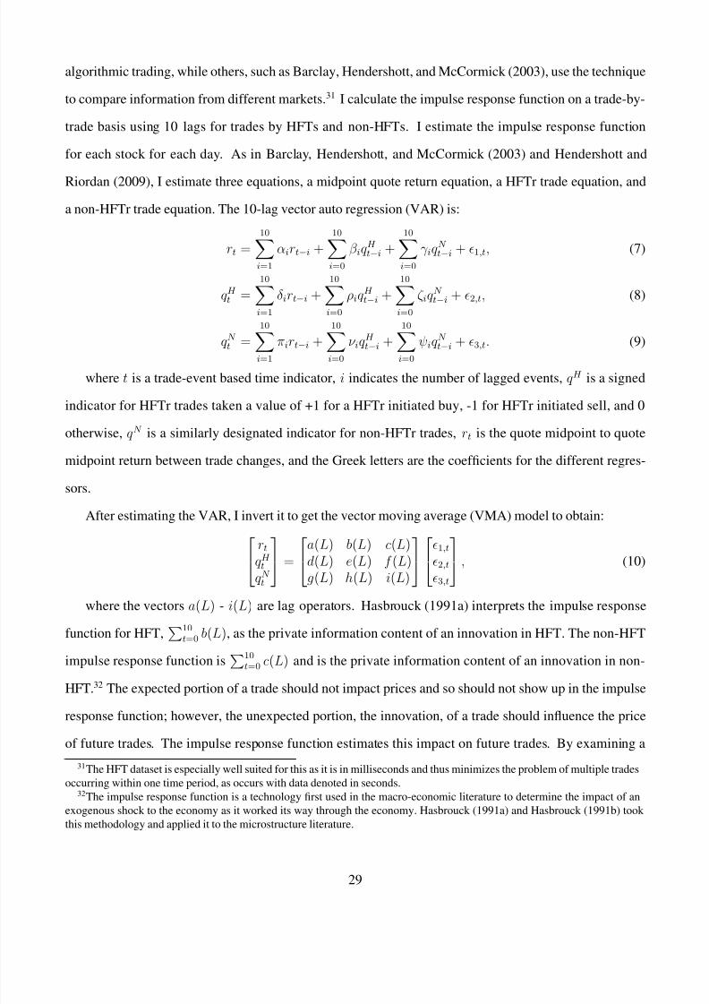


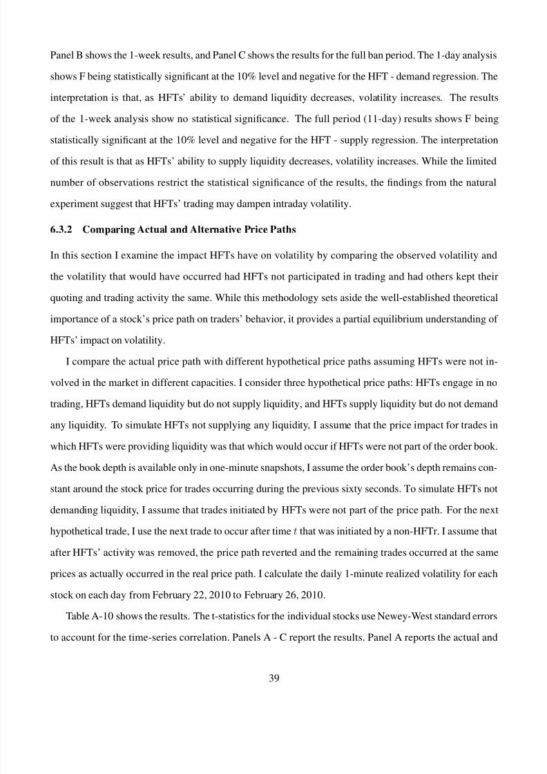


![Ssrn id1862355[1]](https://static.documents.pub/doc/80x56/5464365db4af9f5d3f8b48dd/ssrn-id18623551.jpg)


