STABILITY ANALYSIS OF COMPOUND TCP WITH ADAPTIVE VIRTUAL QUEUES A Project Report submitted by ANAND KRISHNAMURTI RAO (EE09B005) in partial fulfilment of the requirements for the award of the degree of BACHELOR OF TECHNOLOGY in ELECTRICAL ENGINEERING DEPARTMENT OF ELECTRICAL ENGINEERING INDIAN INSTITUTE OF TECHNOLOGY, MADRAS. May 14, 2013
Transcript
STABILITY ANALYSIS OF COMPOUND TCP
WITH ADAPTIVE VIRTUAL QUEUES
A Project Report
submitted by
ANAND KRISHNAMURTI RAO
(EE09B005)
in partial fulfilment of the requirements
for the award of the degree of
BACHELOR OF TECHNOLOGY
in
ELECTRICAL ENGINEERING
DEPARTMENT OF ELECTRICAL ENGINEERING
INDIAN INSTITUTE OF TECHNOLOGY, MADRAS.
May 14, 2013
PROJECT CERTIFICATE
This is to certify that the project titled STABILITY ANALYSIS OF COMPOUND
TCP WITH ADAPTIVE VIRTUAL QUEUES, submitted by Anand Krishna-
murti Rao (EE09B005), to the Indian Institute of Technology, Madras, for the
award of the degree of Bachelor of Technology, is a bona fide record of the
project work done by him under my supervision. The contents of this report,
in full or in parts, have not been submitted to any other Institute or University
for the award of any degree or diploma.
Prof. G. RainaProject GuideProfessorDept. of Electrical EngineeringIIT Madras, Chennai 600 036
Prof. E. BhattacharyaHeadDept. of Electrical EngineeringIIT Madras, Chennai 600 036
Place: Chennai
Date: May 14, 2013
ACKNOWLEDGEMENTS
I would first like to thank Dr. Gaurav Raina for his guidance throughout the
course of this project. He has taught me the importance of framing a scientific
argument along with presenting sound analysis.
Special thanks to Amit Warrier, my batchmate, with whom I have worked
with for a year in completing this project.
I also thank my parents and friends who have been there as a constant
source of support in all my endeavours.
This work was carried out under the IU-ATC project funded by the Depart-
ment of Science and Technology (DST) Government of India and the UK EPSRC
A.1 Bifurcation diagram generated with variation in damping factor θ. The
Hopf is found to be subcritical, and the limit cycles unstable (A.31). 32
iv
ABBREVIATIONS
AQM Active Queue Management
AVQ Adaptive Virtual Queue
C-TCP Compound Transmission Control Protocol
ECN Explicit Congestion Notification
IP Internet Protocol
QoS Quality of Service
RED Random Early Detection
REM Random Exponential Marking
VQ Virtual Queue
v
CHAPTER 1
Introduction
The design of transport protocols influences the performance of Internet ap-
plications. Active Queue Management (AQM) schemes, which aim to provide
timely indications of incipient congestion in the network to end-systems, also
play an important role in Quality of Service (QoS). For an end-to-end perspec-
tive, it is natural to study the interaction of a transport protocol along with
a queue management scheme. Compound TCP (C-TCP) (17) is today widely
implemented in the Windows operating system, and there are numerous pro-
posals for AQMs in the literature.
Queueing delay, in the Internet, is undesirable and specially hurts the per-
formance of delay sensitive applications (11). It is being recognised that net-
work latency is predominantly due to large router buffers without effective
queue management (4). It is difficult for end-systems to compensate for queue-
ing delay, and thus the design of AQMs remains an important aspect of net-
work research. A number of AQM schemes, with different objectives, have
been proposed in the literature. For example, Random Early Detection (RED)
(3) strives for small average queue sizes, Adaptive Virtual Queue (AVQ) (10) tar-
gets a desired link utilisation, Random Exponential Marking (REM) (1) aims for
both small queue sizes and high link utilisation, and CODEL (11) specially aims to
control queueing delay. However, a simple Drop-Tail queue policy is often used
as there is no consensus on an optimal AQM scheme. Drop-Tail, as the name
suggests, simply drops packets that arrive to find a full buffer. For our study,
we focus on a class of virtual queue schemes as they aim to provide early indi-
cations of congestion. We study a non-adaptive Virtual Queue (VQ) (9) and the
Adaptive Virtual Queue (AVQ) (10).
Stability is a key performance metric since feedback, from the network to
end-systems, is usually time delayed. So the analysis of non-linear, time de-
layed, fluid models for transport protocols can help guide protocol or network
parameters, and ensure system stability. For example, non-linear models of
TCP Reno have been studied with different buffer sizing regimes (14) (15), with
the AVQ (10), and also with Drop-Tail (12). These papers have highlighted
that the underlying models can readily lose stability with variations in system
parameters. Hence any analysis should consider both stability and bifurcation
phenomena (6).
In this paper, we analyse a recently proposed non-linear model of Com-
pound (16) with a VQ (9) and with the AVQ (10). Local stability analysis with
the VQ policy reveals that smaller virtual buffer sizing rules help stability. Small
virtual buffers would also lead to lower latency in network routers. We out-
line some guidelines for Compound and network parameters to ensure local
stability. Analysis of the AVQ shows that the system could readily lose local
stability with large delays, high link capacities, and with variations in the AVQ
damping factor. We show that loss of local stability would occur via a Hopf
bifurcation (8), which would give rise to a limit cycle. Based on the analysis, we
note that a virtual queue, with small buffer sizes, could be an appealing queue
management policy.
The rest of this paper is organised as follows. In Section 2, we outline mod-
els for Compound and for virtual queue management schemes. In Section 3
we conduct a stability analysis of the underlying models, and summarise our
contributions in Section 4.
2
CHAPTER 2
Models
In this section, we outline models for Compound and the virtual queue policies
that form the basis for our analysis.
2.1 Compound TCP
The following many flows, non-linear, fluid model has been proposed for a gen-
eralised TCP (14):
dw(t)
dt=(i(w(t)
)− d(w(t)
)p(t− τ)
)w(t− τ)
τ, (2.1)
where w(t) is the congestion window, i(w(t)) is the increase in w(t) per positive
acknowledgement, d(w(t)) is the decrease in w(t) per negative acknowledge-
ment, p(t) represents an appropriate model at the resource, and τ is the feed-
back delay of the TCP flows present. An approximation for the average rate at
which packets are sent is x(t) = w(t)/τ .
In the regime where the queueing delay forms a negligible component of
the end-to-end delay, the following functional forms have been proposed for
Compound (16):
i(w(t)
)=
αw(t)k
w(t), d
(w(t)
)= βw(t), (2.2)
where the parameters α, β and k influence the congestion window’s scalability,
smoothness and responsiveness respectively. The default values of these pa-
rameters are: α = 0.125, β = 0.5 and k = 0.75 (16). It should be noted that the
fluid model is valid when there are many simultaneous TCP flows present in a
high bandwidth-delay product environment.
The simplest queue management policy is Drop-Tail. In a regime where the
number of users are large, and the router buffer sizes are small, a simple fluid
model for Drop-Tail is (15):
p(t) =(x(t)/C
)B, (2.3)
where B is the buffer size and C is the link capacity. For the requisite queueing
theoretic arguments behind the derivation of this fluid model the reader is re-
ferred to (15). Later in the paper, we will outline the impact this queue policy
can have on local stability.
2.2 Virtual Queues
Virtual queues have been proposed as possible queue management schemes;
for an early discussion on virtual queues, see (5). Figure 2.1 shows a basic
virtual queue algorithm. Packets arriving at the queue are added unless the
buffer occupancy exceeds B packets. A virtual queue operates with a service
rate and a buffer size that are both less than the real queue. The algorithm has
a parameter, 0 < κ ≤ 1, which can be tuned by the network provider. Any
arriving packet that would lead to the virtual queue exceeding the value κB is
marked to indicate the onset of congestion. Packets can also be dropped when
the virtual queue crosses the virtual buffer size. End-systems will realise that
their packets have been marked, or dropped at the queue, only after some time
delay. The central idea, for virtual queues, is to start giving early indications of
incipient congestion whenever the rate of offered traffic nears κ.
As a simple model, let us assume that the arriving traffic is a Poisson pro-
cess. The server will then just be an M/D/1/B queue. Consider an M/D/1/B
queue with arrival rate λ and a service every n units of time. The number of
packets in the queue, just after each service, forms a Markov process and it is a
straightforward exercise to calculate the stationary distribution of the process.
So we can readily deduce the packet loss probability and the utilisation of the
server. Such calculations would allow the network provider to better under-
stand the trade-offs between loss and utilisation. As feedback from the queue
to the end-systems is time delayed, another performance metric to consider is
stability.
4
Figure 2.1: The real queue has the capacity to serve C packets per unit time and canhold B packets in its buffer. The service rate and the buffer size of thevirtual queue are scaled down by a factor κ < 1. We assume there is a timedelay of τ time units before any feedback is received by the end-systems.
We now outline a model proposed in (9). Assume that a virtual buffer of
finite size B is maintained, and that from the time of a virtual buffer overflow
to the end of the virtual buffer’s busy period, all packets leaving the real queue
are marked. Thus the virtual buffer’s contents evolve as if overflow is lost,
while the real buffer may or may not have loss. Consider a Gaussian traffic
model: suppose that the workload arriving at the resource over a time period δ
is Gaussian, with mean xδ and variance xδσ2. For this model, the rate at which
workload exceeds the virtual buffer is (7)
L(x, C) = (C − x)
(exp
{2B(C − x)
xσ2
}− 1
)−1
,
and the proportion of workload marked is
p(t) = −d
dCL(x, C
),
which reduces to
p (t) =r(t)er(t) − er(t) + 1
(er(t) − 1)2 ,
where r(t) =2B(C−x(t)
)σ2x(t)
.
For the purpose of analysis and discussion, in this paper, we refer to the
above virtual queue based scheme as a non-adaptive Virtual Queue (VQ). We
now describe the Adaptive Virtual Queue (AVQ) policy which explicitly aims
5
for a desired and high link utilisation (10).
2.3 Adaptive Virtual Queue
Virtual queue management aims to provide early indications of congestion in
the network. This idea was extended to strive for high link utilisation through
the notion of an Adaptive Virtual Queue (AVQ) (10). The AVQ maintains a
virtual buffer whose size is the same as the real buffer. However, there is a
virtual capacity which is less than the real capacity, and this is adapted at the
queues to achieve high link utilisation.
At the packet-level, the AVQ is implemented as follows (10): when a packet
arrives, a fictitious packet is added to the virtual queue, if it is not already
full. If there is an overflow, the packet is discarded from the virtual queue and
marked/dropped in the real queue. At the fluid-level, the marking probability
p(t) is expressed in terms of the rate x(t) as well as the virtual capacity C(t).
The following functional form for the marking probability at the resource was
proposed in (10):
p(t) =max{0,
(x(t)− C(t)
)}
x(t), (2.4)
where this function is differentiable in the region x > C. The virtual capacity C
is updated after every arrival epoch to achieve a desired utilisation. The AVQ
update model, at the router, is
dC(t)
dt= θ
(γC − x(t)
),
where θ > 0 is the damping factor and γ ≤ 1 allows one to choose the desired
utilisation. The factor θ determines how fast the marking probability adapts to
changing network conditions, and its choice is important to maintain stability.
Marking of packets is more aggressive when link utilisation exceeds the desired
level, and less aggressive otherwise. In the functional form (2.4) for the marking
probability, instead of adapting the virtual capacity we could use a static virtual
capacity which is strictly less than the real capacity.
6
Some key features of the AVQ scheme, which are different to the well-studied
RED proposal (3) are as follows: (i) The AVQ marks packets according to the
rate, and not the queue length or average queue length; (ii) The scheme explic-
itly regulates the link utilisation, and not the queue length; (iii) The virtual ca-
pacity is modified by the AVQ update model, and random number generations
at the queue to determine decisions to drop packets are not required.
The Compound fluid model (2.1) coupled with the AVQ update model for
the virtual capacity forms an end-to-end, non-linear, dynamical system. The
stability analysis of this system can help us understand trade-offs for design,
and guide parameters to ensure stable operation. A local stability analysis of
TCP Reno coupled with the AVQ model has been conducted in (10). Our focus
is on Compound TCP, and in the next section we study some stability properties
of both non-adaptive virtual queues and the AVQ scheme.
7
CHAPTER 3
Analysis
In Section 3.1, we study some non-adaptive queue policies and in Section 3.2,
we analyse the AVQ policy with Compound TCP.
3.1 Virtual Queues
We recapitulate the fluid model for generalised TCP (2.1):
dw(t)
dt=(i(w(t)
)− d(w(t)
)p(t− τ)
)w(t− τ)
τ.
The function p(t) represents packet loss or marking probability of packets sent
at time t. The TCP increment and decrement functions are i(w) and d(w) respec-
tively. Recall that the approximation for the average rate of sending packets is
x(t) = w(t)/τ , where τ is the feedback delay of TCP flows. The above model
achieves equilibrium at
i(w∗) = d(w∗)p∗,
where w∗ and p∗ denote the steady state window size and the packet loss respec-
tively. For linearising the generalised TCP equation, consider w(t) = w∗ + u(t),
where u(t) is a small perturbation. This gives
du(t)
dt= −au(t)− bu(t− τ), (3.1)
where
a = −w∗
τ(i′ − d′p∗)
b =1
τ(d(w∗)w∗p′) .
Note that p′ = dp
dw
∣∣w=w∗
; i′ and d′ are similar representations. For Compound
TCP, the functional forms for i(w) and d(w) are outlined in (2.2). Substituting
these expressions into (3.1) gives
a =− (k − 2)αw∗k−1
τ
b =αw∗k−1
τ
w∗p′
p∗,
(3.2)
where α, β and k are Compound parameters. Under the constraints that b >
a ≥ 0 and τ > 0, a sufficient condition for local stability of the linear system (3.1)
is (13)
bτ < π/2. (3.3)
We will refer to bτ as the stability factor. In our build up towards studying a non-
adaptive virtual queue (3.4) with Compound TCP, we first analyse two simple
models for the queue.
In a many flows regime, when the bandwidth-delay product is large and the
router buffers are small, the following fluid-level approximation has been pro-
posed for Drop-Tail queues (15):
p(t) =(x(t)/C
)B.
Here B is the router buffer size and C is the link capacity. In this model there is
no explicit adaptation at the resource, and with Compound there is no control
over link utilisation. In this regime, it is assumed that the queue size fluctuates
so rapidly that TCP cannot control the queue size. In fact, it can only control its
distribution, and hence an explicit representation for the instantaneous queue
size does not feature in the model.
With the small buffer Drop-Tail model, a sufficient condition for local stabil-
ity with Compound is (16)
αw∗k−1B < π/2.
Note that this condition does not depend on the feedback delay or the link
capacity, but depends on the buffer size and the Compound parameters. This
very simple model alerts us to the fact that with large buffers the system could
be harder to stabilise.
9
Load, x/C
Mar
kin
gp
rob
abil
ity,p(x) B/σ2 = 5
B/σ2 = 10
B/σ2 = 20
0.0
0.0
0.2
0.2
0.4
0.4
0.6
0.6
0.8
0.8 1.0
Figure 3.1: Marking probability of the virtual queue model (3.4), with variations inB/σ2. Note that smaller buffer thresholds provide early indications of con-gestion as the load increases.
We now consider a functional form for the resource, outlined in Section 2,
and proposed by (10):
p(t) =max{0,
(x(t)− γC
)}
x(t),
where γ < 1, C is the link capacity, and there is no adaptation at the links.
For this resource model, p(·) represents the proportion of packets overflowing
a large buffer. With this functional form, the corresponding sufficient condition
for local stability with Compound is (16)
βγCτ < π/2.
This condition would clearly be difficult to satisfy with large feedback delays
and high link capacities. The models considered so far suggest that both Com-
pound and network parameters can readily influence stability. In particular,
buffer sizes play an important role and need to be chosen judiciously.
The marking probability for the virtual queue policy outlined in Section 2,
10
under a Gaussian traffic model, is
p(t) =r(t)er(t) − er(t) + 1
(er(t) − 1)2 , (3.4)
where r(t) =2B(C−x(t)
)σ2x(t)
.
Figure 3.1 depicts the marking probability, of this model, for varying val-
ues of the buffer size. Note that smaller values of B provide early indications
of congestion, as the load on the system increases. With k = 1, the sufficient
condition for stability is simply αwp′/p < π/2, at equilibrium. Observe the im-
portant role played by the derivative of the function p in maintaining stability.
Substituting (3.4) into the fluid model for Compound, a sufficient condition for
local stability can be written as
((r∗ − 2) e2r
∗
+ (r∗ + 2) er∗
(er∗ − 1) (r∗er∗ − er∗ + 1)
)C
x∗
2αB
σ2< π/2,
where r∗ = 2B(C−x∗)σ2x∗
. For stability there appears to be a requirement to jointly
design the protocol parameter α and the network parameter B. Larger values
of σ2, the variability of the traffic at the packet-level, appears to help stability. In
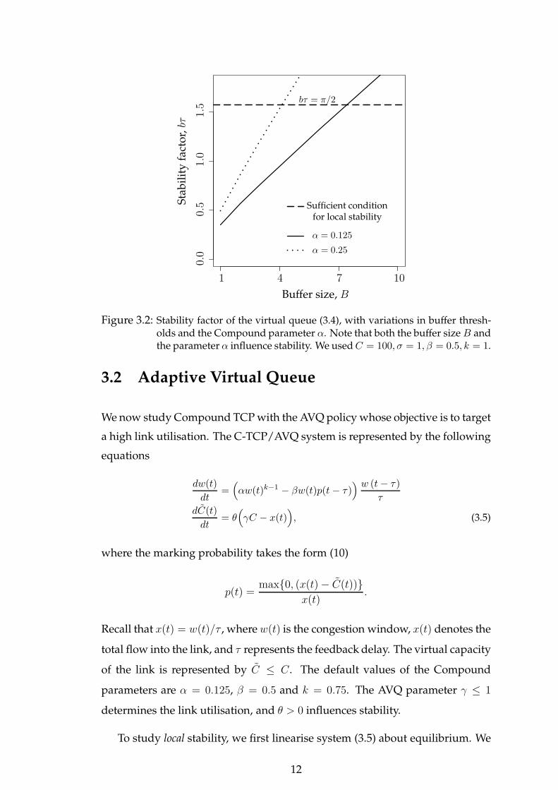
Figure 3.2, we plot the stability factor for different values of the Compound pa-
rameter α and the buffer size B. Note that both B and α have to be judiciously
chosen to ensure stability.
When the buffer threshold levels used to mark/drop packets are large enough
so that queueing delays are comparable to propagation delays, the above mod-
els do not accurately represent the resource. In such a regime, it is important
to model both the instantaneous queue size and the end-system rates in any
dynamic representation. The reader is referred to (14) (15) for the development,
and analysis, of some such models. With the models considered so far, we find
that small buffer sizes help maintain stability, and reduce latency, but there is
no explicit control over link utilisation. High link utilisation is one of the key
aims of the AVQ, and this model will now be analysed.
11
Buffer size, B
Sta
bil
ity
fact
or,bτ
α = 0.125
α = 0.25
bτ = π/2
Sufficient conditionfor local stability
1 4 7 10
0.0
0.5
1.0
1.5
Figure 3.2: Stability factor of the virtual queue (3.4), with variations in buffer thresh-olds and the Compound parameter α. Note that both the buffer size B andthe parameter α influence stability. We used C = 100, σ = 1, β = 0.5, k = 1.
3.2 Adaptive Virtual Queue
We now study Compound TCP with the AVQ policy whose objective is to target
a high link utilisation. The C-TCP/AVQ system is represented by the following
equations
dw(t)
dt=(αw(t)k−1 − βw(t)p(t− τ)
) w (t− τ)
τ
dC(t)
dt= θ(γC − x(t)
), (3.5)
where the marking probability takes the form (10)
p(t) =max{0, (x(t)− C(t))}
x(t).
Recall that x(t) = w(t)/τ , where w(t) is the congestion window, x(t) denotes the
total flow into the link, and τ represents the feedback delay. The virtual capacity
of the link is represented by C ≤ C. The default values of the Compound
parameters are α = 0.125, β = 0.5 and k = 0.75. The AVQ parameter γ ≤ 1
determines the link utilisation, and θ > 0 influences stability.
To study local stability, we first linearise system (3.5) about equilibrium. We
12
then derive the associated characteristic equation, and identify conditions un-
der which the roots lie in the left-half plane (i.e., if Γ is a root, Re(Γ) < 0).
At steady state, dw(t)dt
= dC(t)dt
= 0. Therefore
w∗ = τγC, C∗ = γC
(1−
α
β(τγC)k−2
)(3.6)
which uniquely defines the equilibrium window size w∗ and virtual capacity
C∗ in terms of parameter values. To linearise the coupled system (3.5), let
w(t) = w∗ + u(t)
C(t) = C∗ + v(t),
where u and v are small increments of w∗ and C∗. We get
du(t)
dt=(ατ(k − 2)w∗k−1
)u(t) +
(β
τw∗
)v(t− τ)
+
(α
τw∗k−1 −
β
τw∗
)u(t− τ)
dv(t)
dt= −
θ
τu(t).
To obtain the characteristic equation of this linearised system we look for expo-
nential solutions, v = Aeλt, to get
λ2 + a0λ+ a1λe−λτ + θa2e
−λτ = 0, (3.7)
where
a0 = −α
τ(k − 2)(τγC)(k−1)
a1 = −1
τ
(α(τγC)(k−1) − βτγC
)
a2 = βγC,
are assumed to be positive, and λ = σ + jω.
13
Local stability analysis
Consider the characteristic equation
λ2 + a0λ+ a1λe−λτ + θa2e
−λτ = 0, (3.8)
where a0, a1, a2 > 0 are independent of the feedback delay τ and θ > 0. It is
straightforward to show that when τ = 0, all roots have negative real part and
so the corresponding linear system is stable. The roots of (3.8) are continuous
functions of system parameters. By keeping all the other parameters constant
and increasing τ , one can locate a τ such that at least one of the roots hits the
imaginary axis. Thus for 0 ≤ τ < τ , the roots of (3.8) will all have negative real
parts.
When one of the roots first lies on the imaginary axis, σ = 0. At this point,
let ω = ω0. The real and imaginary parts of (3.8) are, respectively,
ω0a1 sin(ω0τ) + θa2 cos(ω0τ)− ω20 = 0 (3.9)
ω0a1 cos(ω0τ)− θa2 sin(ω0τ) + a0ω0 = 0. (3.10)
Squaring and adding (3.9) and (3.10) yields
ω20 =
(a21 − a20) +√
(a21 − a20)2 + 4(θa2)2
2. (3.11)
Eliminating sin(ω0τ) from (3.9) and (3.10) gives
cos(ω0τ) =(θa2 − a0a1)ω
20
(θa2)2 + a21ω20
, (3.12)
where ω0 is given by the positive square root of (3.11).
So all the roots of (3.8) have negative real parts for τ = 0, and τ is the smallest
positive delay that satisfies (3.12). Hence for all 0 ≤ τ < τ , the corresponding
linear system is stable.
14
Local Hopf bifurcation analysis
Consider a characteristic equation of the form
f(λ,K1, K2, ...., Kn) = 0,
where λ = σ + jω is a complex variable and the Ki’s are system parameters. To
satisfy the Hopf condition (8), with respect to a parameter Ki, we also need to
satisfy the transversality condition, i.e.
Re
(dλ
dKi
) ∣∣∣∣Ki=Ki,c
6= 0,
where Ki,c is the critical value of the parameter Ki beyond which the system is
driven to instability. Note that at Ki = Ki,c the eigenvalues lie on the imaginary
axis, and so σ = 0 and λ = jω0.
The characteristic equation we consider is (3.8), i.e
λ2 + a0λ+ (a1λ+ θa2) e−λτ = 0,
where the critical values of the parameters are obtained from (3.12). We now
verify that the transversality condition is satisfied by the delay τ and the damp-
ing parameter θ.
Feedback delay as the bifurcation parameter
Differentiating (3.8) with respect to τ and rearranging gives
which is always positive since a0, a1, a2 > 0. Thus variations in the damping
factor θ can also induce a Hopf bifurcation. An important parameter in the C-
TCP/AVQ model is θ, and variations in this parameter can lead to limit cycles
in the underlying non-linear system.
We have just shown that a class of linear equations, whose characteristic
equation is represented by (3.8), can lose stability with large delays and with
variations in the parameter θ. Further, both the delay and θ can induce a Hopf
bifurcation.
16
Effective link capacity, γC
Dam
pin
gfa
cto
r,θ
τ = 1τ = 2τ = 10
0
0
1
1
2
2
3
3
4
4
Figure 3.3: Local stability chart of the C-TCP/AVQ model. The area below the curvesrepresents the stable region. Note the trade-offs among the system param-eters to maintain stability. Variations in the AVQ damping factor θ caninduce a Hopf bifurcation. Compound parameters: α = 0.125, β = 0.5,k = 0.75.
Impact of delays on stability of C-TCP/AVQ
The local stability analysis of a TCP Reno/AVQ model was conducted in
(10), which showed that large values of the delay can be destabilising. Follow-
ing a similar style of analysis, one can identify a τ satisfying (3.12) such that
for τ < τ , the C-TCP/AVQ system (3.5) is locally stable. Thus stability of the
C-TCP/AVQ model will not be assured for large feedback delays.
Impact of the damping factor on stability of C-TCP/AVQ
A key parameter in the AVQ policy is the damping factor θ, which deter-
mines the rate of adaptation at the resource. Figure 3.3 shows a stability chart,
highlighting the trade-offs between θ, the feedback delay and the effective link
capacity to maintain local stability. In AVQ, adaptation at the links was intro-
duced to target a high link utilisation at equilibrium. However, our analysis
shows that variations in this parameter can induce a Hopf bifurcation in the
C-TCP/AVQ model.
17
Discussion
Virtual queue policies are attractive as they can provide early indications of
congestion to help end-systems adapt their rates. But this feature alone does not
guarantee stability in the presence of time delayed feedback. We highlighted
that small buffer thresholds help ensure stability, and would naturally reduce
latency. We then exhibited that virtual queues, with small thresholds, have a
stabilising effect but these thresholds have to be chosen in conjunction with
Compound parameters. So stability can be ensured, but there is no explicit
control over link utilisation.
The AVQ policy aims to achieve a desired link utilisation at equilibrium,
and introduces a damping factor θ at the resource. However, at sufficiently
high feedback delays the C-TCP/AVQ model is prone to losing local stability.
In fact, an increase in θ can induce a loss of stability via a Hopf bifurcation.
From the analysis in the paper, our recommendation is that a non-adaptive
virtual queue policy, with small virtual buffer sizing rules, is an attractive queue
management scheme.
18
CHAPTER 4
Outlook
End-systems can detect congestion in the network via the loss of packets or by
increased latency. Today, transport protocols like Compound TCP use both loss
and delay as feedback to manage their flow and congestion control algorithms.
Queueing delay, specially at network routers, is increasing which can be detri-
mental to services and applications that require low latency for good quality
of service (11). Large buffers, without effective queue management, contribute
fairly substantially to latency in the network (4). A plausible way to reduce la-
tency from router buffers is to design appropriate Active Queue Management
(AQM) schemes. We note that feedback to end-users is always time delayed,
and so stability is a key performance metric.
Contributions
We studied some stability properties of a fluid model of the widely de-
ployed Compound TCP with virtual queue policies. Our investigation of a
non-adaptive Virtual Queue (VQ) revealed that small virtual buffer sizing rules
would help stability, and also reduce network latency. We showed that Com-
pound parameters can influence stability, and that unguided choice of parame-
ters can easily violate the stability conditions. Analysis of the AVQ showed that
large delays, high link capacities, and variations in the AVQ damping parame-
ter can render the system in a locally unstable state. Additionally, we explicitly
characterised the loss of local stability to occur via a Hopf bifurcation.
With a non-adaptive VQ we could have low latency and a stable system,
but no explicit control over link utilisation. The AVQ is designed to target a
desired and high link utilisation, but the AVQ damping factor can readily in-
duce a Hopf bifurcation. Thus a simple non-adaptive virtual queue policy, with
small router buffers, appears to be an appealing choice for queue management.
Avenues for further research
When a Hopf bifurcation condition is just violated, we can expect a limit
cycle branching from the fixed point (6). It would be important to determine if
the bifurcating limit cycle, with the AVQ, is asymptotically stable. One could
follow the style of analysis presented in (8) (13) to address this question. Feed-
back to end-systems could also be in the form of Explicit Congestion Notifica-
tion (ECN) (2). ECN allows routers to mark an IP packet when resources start
to get congested. Thus end-systems do not need to rely only on packet loss, or
latency, to infer the state of congestion in the network. It is natural to inves-
tigate the benefits of a virtual queue based scheme, with small router buffers,
employing ECN marks.
20
APPENDIX A
Analytical characterisation: stability and periodicity
of bifurcating solutions
In Section 3, we proved that variations in the damping parameter θ can induce
a loss of stability in the C-TCP/AVQ system via a Hopf bifurcation. This leads
to the emergence of limit cycles. The next question to address would be the
nature of the Hopf and the stability of the ensuing limit cycles.
A Taylor expansion of the C-TCP/AVQ model (3.5) about the equilibrium
point (3.6) yields
du(t)
dt= −
α
τu(t)− βC∗u(t− τ) + βw∗v(t− τ)
−β
τu(t)u(t− τ)−
βC∗
w∗(u(t− τ))2
+ βu(t)v(t− τ) + βu(t− τ)v(t− τ)
dv(t)
dt= −
θ
τu(t).
We introduce an exogenous non-dimensional parameter κ = κc+µ, where κc =
1, and the Hopf bifurcation occurs at µ = 0. Substituting b1, b2, bc, b12, b22, b1c
and b for −α/T, −βC∗, βw∗, −β
τ, −βC∗
w∗, β and − θ
τrespectively, we have:
du(t)
dt= κb1u(t) + κb2u(t− τ) + κbcv(t− τ)
+ κb12u(t)u(t− τ) + κb22 (u(t− τ))2
+ κb1cu(t)v(t− τ) + κb1cu(t− τ)v(t− τ)
dv(t)
dt= bu(t).
(A.1)
We will now perform calculations that will enable us to address questions
about the form of the bifurcating solutions of (A.1) as it transits from stability
to instability via a Hopf bifurcation. We follow the style of analysis provided in
(8).
Consider the following autonomous delay-differential system:
d
dtu(t) = Lµut + F(ut, µ) (A.2)
where t > 0, µ ∈ R, and for T > 0,
ut(θ) = u(t + θ) u : [−T, 0] → R2, θ ∈ [−T, 0].
Lµ is a one-parameter family of continuous (bounded) linear operators. The op-
erator F(ut, µ) contains the non-linear terms. Further assume that F is analytic
and that F and Lµ depend analytically on the bifurcation parameter µ for small
|µ|. Note that (3.5) is of the form (A.2), where u = [u, c]T . The objective now is
to cast (A.2) into the form:
d
dtut = A(µ)ut +Rut (A.3)
which has ut rather than both u and ut.
First, we transform the linear problem du(t)/dt = Lµut. From the Riesz
representation theorem, there exists an n × n matrix function η(·, µ) : [−T, 0] →
Rn2
, such that the components of η have bounded variation and for all φ ∈
C[−T, 0],
Lµφ =
∫ 0
−T
dη(θ, µ)φ(θ).
In particular,
Lµφ =
∫ 0
−T
dη(θ, µ)u(t+ θ). (A.4)
Observe that
dη(θ, µ) =
(κb1δ(θ) + κb2δ(θ + τ))dθ κbcδ(θ + τ)dθ
bδ(θ)dθ 0
satisfies (A.4). For φ ∈ C[−T, 0], define
A(µ)φ(θ) =
dφ(θ)dθ
,
∫ 0
−Tdη(s, µ)φ(s) ≡ Lµφ,
θ ∈ [−T, 0]
θ = 0
(A.5)
22
and
Rφ(θ) =
0,
F(φ, µ),
θ ∈ [−T, 0]
θ = 0.
(A.6)
As dut/dθ = dut/dt, (A.2) becomes (A.3) as desired.
The bifurcating periodic solutions u(t, µ(ǫ)
)of (A.2) have amplitude O(ǫ)
and non-zero Floquet exponent B(ǫ), where the expressions for µ and B are
given by
µ = µ2ǫ2 + µ4ǫ
4 + · · ·
B = B2ǫ2 + B4ǫ
4 + · · · .
The sign of µ2 determines the direction of bifurcation. µ2 > 0 represents a
supercritical bifurcation and µ2 < 0, a subcritical one. The sign of B2 determines
the stability of the limit cycle. Asymptotic orbital stability is maintained if B2 <
0, and it is unstable otherwise. These coefficients will now be determined.
We only need to compute the expressions at µ = 0, hence we set µ = 0. Let
q(θ) be the eigenfunction for A(0) corresponding to λ(0), namely
A(0)q(θ) = iω0q(θ)
To find ω0 and q(θ), let q(θ) = q0eiω0θ, where q0 = [1, q02]
T . Substituting this in
the above equation and using the expression for A as in (A.5), we get:
ω0 =
√√√√(b22 − b21) +
√(b22 − b21)
2+ 4b2c
2
q0 =
1
biω
≡
q01
q02
(A.7)
Define the adjoint operator A∗(0) as
A∗(0)α(s) =
dα(s)ds
,
∫ 0
−TdηT (t, 0)α(−t),
s ∈ [0, T ]
s = 0.
23
Note that the domains of A and A∗ are C1[−T, 0] and C1[0, T ] respectively. As
A(0)q(θ) = λ(0)q(θ),
λ(0) is an eigenvalue for A∗, and
A∗(0)q∗ = −iω0q∗
for some non-zero vector q∗. For φ ∈ C[−T, 0] and ψ ∈ C[0, T ], define an inner
product
〈ψ,φ〉 = ψT(0)φ(0)−
∫ 0
θ=−T
∫ θ
τ=0
ψT(τ − θ)dη(θ)φ(τ)dτ. (A.8)
Then, 〈ψ,Aφ〉 = A∗〈ψ,φ〉 for φ ∈ Dom(A) and ψ ∈ Dom(A).
Let q∗(s) = Deiω0s be an eigenvector of A∗ corresponding to eigenvalue
−iω0. We will now find D such that the eigenvectors q and q∗ satisfy conditions
〈q∗, q〉 = 1 and 〈q∗, q〉 = 0. These two equations can be solved for variables D1
and D2, where D = [D1, D2]T .
Following the analysis similar to the one leading to (A.7), we find that
q∗0 = D1
[1 b1bc+iω0bc
−bbc+ib2
]. (A.9)
Using the expression (A.8) for the inner product and on solving for D1, we get