Stability and Error Estimation for Component

Adaptive Grid Methods

Joseph Oliger and Xiaolei Zhu

The Research Institute of Advanced Computer Science is operated by Universities Space Research

Association, The American City Building, Suite 212, Columbia, MD 21044, (410) 730-2656

This work was begun with support from the Office of Naval Research under contracts N00014-89-J-185-P00006 and N00014-90-J-1344-P00005 and completed with support from the National ScienceFoundation under grant DMS-9318166 and NASA under contract NAS2-13721.

https://ntrs.nasa.gov/search.jsp?R=19950005470 2018-06-13T17:30:44+00:00Z

Abstract

Component adaptive grid (CAG) methods for solving hyperbolic partial differen-

tial equations (PDE's) are discussed in this paper. Applying recent stability results

for a class of numerical methods on uniform grids, the convergence of these methods

for linear problems on component adaptive grids is established here. Furthermore,

the computational error can be estimated on CAG's using the stability results. Using

these estimates, the error can be controlled on CAG's. Thus, the solution can be

computed efficiently on CAG's within a given error tolerance. Computational results

for time dependent linear problems in one and two space dimensions are presented.

1 Introduction

Component adaptive grid methods for solving hyperbolic PDE's were introduced in

the early 1980's. An overview of the method is given in Section 2. More details can be

found in Berger and Oliger [2], and Berger [1]. However, the grid structure used in this

paper is different from the one Berger used. As discussed in Section 2, stair step grids

like those of Chesshire and Henshaw [4] are used in our CAG methods here, instead

of rotated rectangular grids. One major component of the adaptive strategy is to

estimate the local truncation error at each grid point, then refine where the estimated

errors are larger than a given tolerance 5. The smaller _ is, the smaller the final error

is expected to be in some weighted L2 norm. However, no quantitative relationship

between these two kinds of errors had been established. Recently, new stability results

have been developed by Pelle Olsson [6] which allow us to establish such a relationship

for large classes of problems and methods. The results can be applied to various classes

of problems, e.g., those of hyperbolic, parabolic and hyperbolic-parabolic type, using

a large class of numerical methods on uniform grids. As we will see in Section 3, the

structures of component adaptive grids allow us to define the solution on piecewise

uniform grids. So the stability theories can be applied on CAG's. Convergence for

linear problems using these methods on CAG's is proved in Section 3. Also the

tolerance _ on local truncation error is estimated in term of the tolerance c on the

final error. Furthermore, the results in Section 3 will also help us estimate the final

error using simple quadrature, and serve us as guidelines on developing strategies

for CAG methods, since we have a very good understanding of the sources and the

magnitudes of various computational errors. Finally, some computional results for

time dependent problems in one and two space dimensions are given in Section 4.

2 An Overview of Component Adaptive Grids

We first introduce some notation for our discussion. Suppose the problem we wish to

solve is written as

ut = L u + f on f_× [0, T] (1)

u(0) = u0 on (2)Bu = b on 0f_×[0, T] (3)

where fl C R d is a bounded domain in physical space, L is a spatial partial differetial

operator on F/and u E/_. We assume this to be a well-posed initial-boundary value

problem which is defined in Section 3. Let F/h, Ol2h and [0, T]k be the discretizations of

_, OF/and [0, T], respectively. In Section 3, these discretizations are defined precisely

2

for our component adaptive grids. For the time being, we can consider them as

general grids.

Let Vh be a grid function defined on F/h × [0, T]k. We will discuss the use of

finite difference methods on these grids. Without loss of generality, and avoiding

complicated notation, we write our methods in explicit one-step form as

vh(t + k) = Lhvh(t) + k f_(t) on F/hx[0, T]k (4)_(0) = _o_ o_ F/_ (5)

Bhvh(t) = bh(t) on 0F/hx [0,T]k (6)

where we use subscripts to denote projections of functions onto the appropriate grids

and discretizations of operators on these grids. If Uh is the projection of the exact

solution of the above system onto F/h, then

uh(t + k) = Lh uh(t) + k fh(t) + k'rh on _h × [O,T]k (7)

where Th is the local truncation error. This notation will also be used on the piecewise

uniform grids which we will discuss next.

2.1 Composite Grids

In real applications, the physical domains often have complicated geometries. In order

to use finite difference schemes on these domains, we decompose the physical domain

and transform the parts into computational domains. However this topic is not the

focus of this paper. Here only a brief introduction is given to make our presentation

self contained. Details can be found in Chesshire and Henshaw [4], Venkata, Oliger

and Ferziger [8], and Venkata [9].

We begin by forming a base composite grid

Go= [_Jao,j (S)J

which will be characterized by a discretization parameter h0.

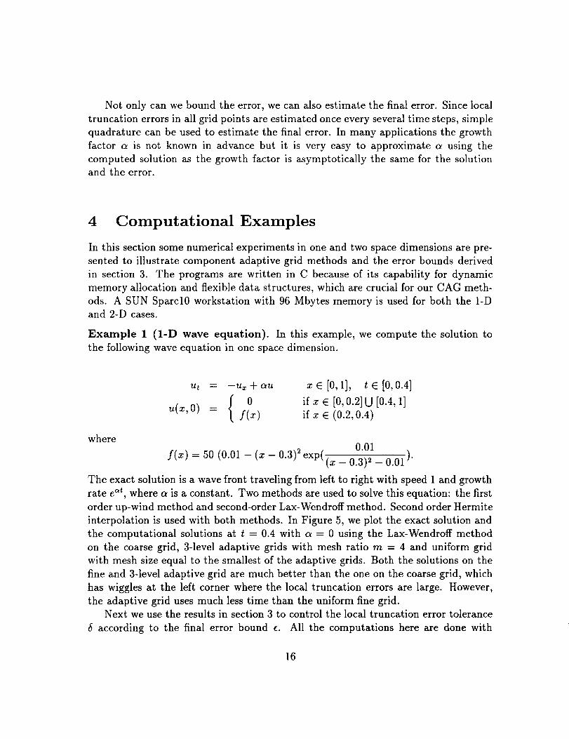
This is well illustrated in Figure 1 where Go consists of the component grids Go,l,

G0,2, and G0,3. G0,: is a stair step grid with grid lines parallel to the coordinate axes.

Such grids are called regular grids.

Definition 1: A regular grid is a connected stair step grid of uniformly spaced

points in each coordinate direction, and its grid lines are parallel to the coordinate

3

axesin either physical or computational space.

No coordinate transformation is neededto solvethe equation on regular grids inphysical space. The curvilinear grids G0,1 and G0,3 are defined by specifying their

boundaries and cuts. Regular girds in computational space are then mapped onto

these grids in physical space using coordinate tranformations. To reduce clutter in

Figure 1 , grids G0,1 and G0,3 are shown only in computational space. The component

grids are chosen to obtain a sufficiently accuate representation of 0R by Oglh. ho is

an estimate of the step size required to obtain a sufficiently accuate approximation of

the solution over at least some specified fraction of the domain. The difficult problem

here is to generate grids on the boundaries. The B_zier family of curves and surfaces

are used to generate boundary grids in 2-D and 3-D, respectively (see [8] and [9]).

G0, 2

G1,1

G0,3

G1,2

0,1G

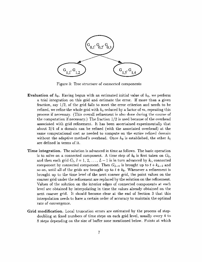
1,3 G1,4

I I I I I I I I I I 1 I I I I I I I I I I I I 1 I I I I iaman"

lllllllllllllllllllllllllllllllll_ i]lllllllllllllllllllllllllllllllJl_

Figure 1: Adaptive Composite Grid Structure

2.2 Component Adaptive Grids

The component grids mentioned in Section 2.1 are specified to describe the domain

and its boundaries. Next, we will discuss the use of adaptive grids which are created

and destroyedduring the courseof the computation in order to maintain sufficientaccuracythroughout the entire domain.

During this process,wewill createL - 1 additional refinement levels of composite

grids Gl on top of the base grid Go. So the whole grid system can be written asfollows:

L-1

U a, (9)I=0

where at each level l, we have

= U c ,j. (10)j

These will have spatial discretization parameters hi = ho/m t, where m might range

from 2 to 10 depending on the problems being solved. According to Berger and Oliger

[2], m = 4 is a reasonable choice for many hyperbolic problems. We usually let L be

2, 3 or 4. As dictated by the nature of the problem and numerical algorithm, we main-

tain an appropriate relationship between the spatial and the temporal discretization

parameters, ht and kt. In particular, for problems which are essentially hyperbolic in

character, we usually use the same mesh ratio on all levels, i.e.,

= kt/ht = constant. (11)

Another very important feature for our adaptive grids is that the grids are level

nested, i.e., the region Gl is fully contained within the region Gt-1. See the shaded

refined grids Ga,x, G1,2, G1,3 and G1,4 in Figure 1. Since these grids have the same mesh

ratio, they have the space-time structure illustrated in Figure 2. We take several time

steps on the finer grid for each time step on the coarser grid.

:.,,., ======================:.:+: :.::.::i:i:|::::::::::::::,:::::::|:::::::|......•--'- ..:...:i:,:.:._t+:.:. +:.:. ::.:

::::::::::::::::::::::::::::::::::::::::::::::::::::::::::::::::::

:::::::::::::::::::::::::::::::::::::::::::::::::::::::::::::::::::::::::::::::::::::::::::::::::::::::::::::::::::::::::::::::::::::::::::::::

:::::::::::::::::::::::::::::::::::i::i::::::::::::::::::::::::::i::i::ii_-E_::_i_::_)::_::_iii_)i_::::::::::::::::::::::::

--lip-

x

Figure 2: Space-time grid structure

We generate the refinement grids in response to computed estimates of local trun-

cation error. If the solution is sufficiently smooth, a variant of Richardson extrapola-

tion, call step-doubling, can be used to estimate the local truncation error rh at each

5

point of the grid. For simplicity, we consider the one-step explicit difference scheme

described in equations (4) to (7). We define the operator Qh as follows:

Qhuh(x,t) = Lhuh(x,t) + kfh(t). (12)

If the solution is smooth enough, then the local truncation error can be written as

kT.(x,t) = uh(x,t + k)--Qhuh(x,t)

= k(kq'a(x,t) + M2b(x,t)) + ]gO(]gql+l "4-h q2+1)

---- kT + kO(k q'+l + h q_+l) (13)

where the leading term is denoted by kr. If u is smooth enough and we take two time

steps with the operator Qh, to leading order the error is 2kv,

uh(x,t + 2k)- Q_uh(x,t)= 2kr + kO(k ql+l .3ff hq2+l). (14)

Let Q2h be the same difference operator as Qh but based on mesh widths of 2h and

2k. Also, assume the order of accuracy in time and space are equal, ql = q2 = q.Then

uh(x,t + 2k)- Q2huh(x,t) = 2k((2k)qa(x,t) + (2h)qb(x,t)) + O(M +2)

= 2q+lkr + O(hq+2).

Subtract equation (14) from equation (15) and use equation (13) to obtain

(15)

_-h(X,t) = Q2hUh(X't) -- Q2huh(x,t)k(2 q+l -- 2) + O(M+'). (16)

The restriction that the accuracy in time and space is the same is not a severe one.

For details see Berger [1]. For nonsmooth solutions we no longer have an accurate

error estimate. However, the Richardson estimates still provide a good criterion for

refinement since the estimates will be large near a singularity.

2.3 Adaptive Grid Generation and Integration

With the basic background mentioned above, we will now explain the adaptive grid

generation and integation processes. It is important to organize the data structure

for the adaptive composite grid in terms of connected components, i.e., connected

sets of component grids at each level. See Figure 3 for the tree representing the grid

structure in Figure 1. Details on implementation can be found in [1] and [2].

6

Figure 3: Tree structure of connected components

Evaluation of h0. Having begun with an estimated initial value of h0, we perform

a trial integration on this grid and estimate the error. If more than a given

fraction, say 1/2, of the grid fails to meet the error criterion and needs to be

refined, we refine the whole grid with h0 reduced by a factor of m, repeating this

process if necessary. (This overall refinement is also done during the course of

the computation if necessary.) The fraction 1/2 is used because of the overhead

associated with grid refinement. It has been ascertained experimentally that

about 3/4 of a domain can be refined (with the associated overhead) at the

same computational cost as needed to compute on the entire refined domain

without the adaptive method's overhead. Once h0 is established, the other ht

are defined in terms of it.

Time integration. The solution is advanced in time as follows. The basic operation

is to solve on a connected component. A time step of k0 is first taken on Go,

and then each grid Gl, l = 1, 2, ..., L - 1 is in turn advanced by kl, connected

component by connected component. Then GL-1 is brought up to t + kL-2 and

so on, until all of the grids are brought up to t + k0. Whenever a refinement is

brought up to the time level of the next coarser grid, the point values on the

coarser grid under the refinement are replaced by the solution on the refinement.

Values of the solution on the interior edges of connected components at each

level are obtained by interpolating in time the values already obtained on the

next coarser grid. It should become clear at the end of Section 3 that this

interpolation needs to have a certain order of accuracy to maintain the optimal

rate of convergence.

Grid modification. Local truncation errors are estimated by the process of step-

doubling at fixed numbers of time steps on each grid level, usually every 4 to

8 steps depending on the size of buffer zone mentioned below. Points at which

7

the error criterion is near violation are flagged, clusters of the flagged points are

formed, and refinements overlaying the clusters are constructed. Once a new

component grid is defined, the solution at previously refined points is retained,

and the solution at all other points is obtained by interpolation accurate to a

certain order from the parent grid. (At the initial time, in contrast, the solution

at each refinement level is obtained from the initial data u0.) The refined grids

are constructed with buffer zones around the flagged points, sufficiently wide

so that a phenomenon requiring refinement cannot move out of the refined area

before the next regridding. This is necessary to maintain accuracy. The grids

are moved by constructing a new grid and deleting the old one, see Figure 2.

Each refinement level is in turn refined as necessary in the same manner, until

the finest level has been reconstructed.

3 Stability, Convergence and Error Estimation

3.1 Stability

As mentioned in the beginning of section 2, the original and discretized problems we

deal with are formulated in equations (1)- (3) and equations (4) - (6), respectively.

Once again, we recall that subscripts h and k are used to represent the discretized

domains, operators and variables. Our goal is to use CAG's to compute the solution

such that the error is bounded by a given tolerance ¢, i.e.,

Ileh(T)ll_h <_ (17)

where II. Ilab is some discrete norm and eh(t) is the discrete error function, both tobe defined later.

Before discussing the discrete case, we want to assume that the original initial-

boundary problem is well-posed. The well-poseness of a large class of problems is

discussed in Kreiss and Lorenz [5]. For hyperbolic and parabolic problems, we use

the following definition.

Definition 2: The initial-boundary value problem defined by equations (1) - (3) is

well-posed if there exists an unique solution which satisfies the following estimate

ilu(.,t)ll _ < Ke_t(llu0(.)ll_ + iif(.,.)l _ 2_ I_×[0,,]+ lib(',")110_×[0,,]) (18)

where K and a are constants, t E [0, T] and the norms are defined in the usual way:

Ilu(-,t)ll_ = [ lu(x,t)12dx (19)

/0t/ Ib(x, r)l=ds dr (20)IIb(.,')llo_×[o4 =

f [ If(z,r)12dx dr (21)Ilf(.,.)ll_×[04d0 Jf_

and l" l is the standard L2 norm in R n, i.e., lul2 = u*u.

In order to achieve our goal, some stability results, which are similar to the well-

poseness of the original problem, are needed for the finite difference schemes. In his

report, Pelle Olsson [6] used energy methods and summation by parts (a discrete

version of integration by parts) to establish stability estimates on uniform grids for

the semi-discretized case, i.e., when only the spatial domain is discretized. The spa-

tial discretizations used are centered differences with various orders of accuracy. To

overcome the difficulty of general boundary conditions, some projection matrices are

used so that the solution can be projected into the solution space where the bound-

ary conditions are satisfied. These results hold for a large class of linear problems,

e.g., hyperbolic, parabolic and some mixed types. Although only 2-D problems were

considered in his report, the results can be easily generalized to higher dimensions.

We assume the following stability estimates holds for our finite difference methods on

the uniform mesh. This is consistent with the results of Olsson [6].

Definition 3: A finite difference method for the initial-boundary value problem

(equations (4) to (6)) on a uniform grid is stable if

_ 2 b 2Ilvh(t)llgh < K_(lluo_llg_ + IIAIl_hx[o4_+ II hlloa.x[o,t],) (22)

where K and a are independant of k and h, t C [0, T] and the discrete norms are

weighted L2 norms in general. Here we can assume they have the following form:

Ilvh(t)ll_%_ = _ halvh(x_,t)l _ (23)xj Eg_h

Ilbhllgahx[o4,= _ khd-'lbh(zj,t,)l _ (24)zj Ea9h,t, e [O,t]k

IlAll%,x[o4_ = _] khdlfh(xj,ti)] 2. (25)xjEt2_,tiE[O,t]k

Here we recall d is the dimension of domain f_. And we assume flh is a uniform

rectangular grid in the above definition. In general the underlying discrete innerprod-

uct must be modified, see Olsson [6]. In order to simplify the notation, a single index

j is used for the grid points in d dimensions. For the same reason, we use the same

K and a in Definition 2 and 3. In fact, they are not necessarily the same constants.

However, in order to approximate the original problem better, it is desirable to have

the a in the discrete case to be close to the one in original problem. This is refered

to as strictly stable in Olsson's report. It can be shown that the two a's are equal up

to an error of order O(h) in his estimates.

Before deriving the error estimates for CAG methods, another assumption is nec-

essary. We will assume K = 1, where K is the coefficient in equation (22). According

to the stability results of Olsson, K > 1. Let's see what happens if K > 1. Since

adaptive grids are used, the stability bound in Definition 3 is used whenever a regrid-

ding process is carried out. We consider a simple case with homogeneous boundary

conditions and zero forcing term. Assume that we regrid at every time step, then we

get

K_kllvh(O)ll_

K2_kllvh(O)ll_

So at time T, the growth bound looks like

[[vh(T)ll_ _ KT/ke_TIIvh(O)I[_

This bound is useless unless K < 1 +O(k). However, we can always absorb K into the

term e_'t with a new a if K < 1 + O(k). Therefore, we take K = 1. Fortunately, many

problems we are interested in have this nice property since they describe physical

phenomena which conserve energy.

3.2 Convergence

Now, we are ready to define _h in the case of CAG's. We use the notation G to

represent this discretization of the original domain. Given a composite component

grid, which is defined in Section 2 and may contain several levels of subgrids, the

domain where the computational solution vector Vh is defined can be constructed in

the following way. Suppose there are L levels of subgrids Go,..., and GL-1, and every

component grid Gl.j is a regular grid. Then Vh is defined spacially on the set

L-2

a= a,_,_,U ( U (a,_,-a,)) (26)1=1

lO

where GI-1 - Gt is the complement operation. This set is well defined in the 1-D

case since we enforce Gt C Gt-1 and there is no overlapping among the subgrids of

the same level. But in higher dimensions there may be overlapping areas in Gl. The

above definition is still valid if the solution vector is uniquely defined on each Gt.

All the components in G_ will have errors of the same magnitude. So the solution

vector can be defined using any one of the grids in the overlapping area. Suppose

Gl,jl, Gtd_, ..., G_,j, have an overlapping area, where jl < j2 < ... < j,_. Then

the solutions of Gl,jl are used in the overlapping area. In other words, by using the

smallest-indexed grid in the overlapping area, we can uniquely define the solution

vector on every level. Then, equation (26) is well defined in higher dimensions and vh

is defined on a piecewise uniform mesh. We also notice that the set G is a function of

time, i.e., G = G(t), because it may change whenever a regridding process is done at

any level. By this observation, we can define Vh on the interval [0, T]. In fact, Vh is a

piecewise constant solution function on [0, T]. Its solution values change only when a

integration or regridding process is carried out at any level. Because G is a piecewise

uniform grid, we can define OG to be the union of all the boundaries of these uniform

grids. The discrete norms defined in equations (23) to (25) can be easily generalized

as follows:

Ilvh(t)l[_(O = __, hd(j)lVh(Xj,t)l 2 (27)zj • G(t)

2 _ a-1 x (28)libhlt0c<r)×[0,r]- Z _2 k,(,)h,(j)ibh( j,t,)l 2t, •[O,T]k xj COG(t)

i 2 = d (29)Ifhllc(r)×[0,r] _ Z k'(')h'o)lh(x"t')l 2t, •[O,T]k xj •G(t)

where hz(j) is the mesh szie of the grid to which the grid point xj belongs. For

simplicity, we assume the mesh sizes in all directions in a component grid are equal.

Now we define the solution error eh on the same domain of Vh as follow:

_h(t) = vh(t) - uh(t) (30)

where Uh is the projection of the exact solution onto G.

On each section with uniform grid G,,._ilo_m and time interval [to, tx], the error eh

satisfies following error equations:

eh(t + k) = Lh eh(t) + k ri,_, on a_..]o_m × [to, q],

eh(0) = e0h on Gunilorm,

B_eh(t) = _'bd_ on OG_qo.. x [t0,t_].

(31)

(32)(33)

Since linear problems are considered here, the error equation is the same as the

discrete equation for Vh except the forcing and boundary terms are replaced by the

11

local truncation errors. Thus, the growth bound for eh on the piecewise uniform grids

can be obtained by applying the stability results in Section 3.1.

Next we are going to prove the error estimation for CAG methods using induction

on the number of grid levels. First we consider the case of only one level of grids.

Since it is piecewise uniform, we can use the result in equation (22) on each piece

of uniform grid. Also we bound the error on grid G by the summation of the errors

on the pieces of uniform grid because of the way we define G and the norm lI" I la.

Assume the local truncation errors of the numerical method used have the accuracy of

order p at interior and boundary points. The initial values are also assumed accurate

to order p. Then from equation (22), it is easy to see following error bound holds:

II h(T)II Coe Th2op (34)

where _< means "asymptotically less than", since only the leading terms of the trun-cation errors are estimated here.

Now we assume that equation (34) holds for L levels of grids. Next we will show

it for L + 1 levels. Because of the way we construct the subgrids which are nested

in their parent grids, we only need to consider two levels. By induction, we know

the error on the finer of the two levels is of order O(h_), so we can always write it as

O(h_). Assume the computation starts at t = to, we have the following error bound

until we regrid at t = tl,

Ileh(tx)ll + IIT 'lla×t ,-,0]+ IITbd 2II0a×t,l-,0j) (35)

where ri,_t is the local truncation error in the interior points, and rbd,._, is the truncation

error introduced at the boundaries, which include the exterior boundaries OG _:t and

the interior boundaries OG i'u. Suppose a pth order method is used in the interior

points. On the exterior boundaries and the interior boundaries, suppose we use qth

and rth order methods, respectively. Then the following estimates are obtained:

= (3s)

I_(OG) = E hd(j_ • (39)

I 2I ,.,llcxt,,-,01 (36)2 2r int t¢_ k2h 2q" [_¢_ext_lt to) + C3koh0 _(Oa )( 1 - to) (37)

where #(.) is a measure of the grid G and its boundaries which are defined as follows:

E %,x_EG

xj 60G

At t = tl, the regridding process is executed on this regular grid. Another type

of error n=it, which is due to the initialization of the subgrids using interpolation, is

12

introduced. Let's assumethis processhaserror of O(h_). Thus, after the regridding

process at t = tl, we will have following error estimate:

Ileh(t,+)ll_ < Ileh(t,)ll_ + Ilr_..tll_

< lleh(tl)ll + C4h s. (40)

If equations (35), (36) and (37) are substituted into equation (40), and the fact that

hl/kt = constant is used throughout computation, the total error after the regridding

process at t = tl is

Ileh(tl+)ll_ < + Clh2op#(G)(tl - to) + C2h2o(q+l)#(OGe_t)(tl - to)

+Cah2o(T+')#(OGint)(t, - to)} + C, hg'. (41)

where the subscript + on the left hand side of equations (40) and (41) represents the

fact that the regridding process is done at time t = t,. All the terms in equation

(41) are under control except #(OG {'_t) since we do not know how many subgrids are

generated. The following lemma gives a bound on tt(OGi'_t).

Lemma 1: Let Go be a regular grid in R e. Assume that there are L levels of grids

Go,..., GL-1 with the refinement ratio rn = hj/hj+l. Then the following asymptotic

inequality holds for small h0.

L-1

#(UUOG, d) < holC(d,m,L)#(Go) (42)l=l j

where C(d, m, L) is a constant depending on d, rn, and L.

Proofi Since a regular grid is an union of rectangular grids, without loss of gen-

erality, we can assume that Go is a rectangular grid. First we bound the boundaries

of G1. According to the discussion in section 2, it can be shown that the case with

largest interior boundaries as h0 is very small for d = 2 is in Figure 4. So, it is easy

to see that the following bound holds:

tt([..JOGa,j) _ 2dhao-'tt(G°)j 2dhdo

1 2d= h o _g(Go).

So, for each level l, 1 = 1,2,...,L - 1, we have

1 2d12(UOGI,j) <,_ hl__l--_#(al-1)

J

2d mr1z

13

Figure 4: The casewith largest interior boundariesin 2-D

Therefore,wehave

L-1

,.(U U ac,,_)/=1 j

2d 1 m (m_L_2_< ho'_-_(Co)( +(_)+...+,2d, ,

ho'C(d,m,L)#(Go)

where

241 - (_)--) (43)C(d,m,L)= 2d(1_ _ )

Remark: The above lemma tells us is that, under the worst senerio, the error term

involving #(c3G i'_t) may lose one order of accuracy. However, the bound in the lemma

is very pessimistic. In most situations, the number of subgrids is usually quite small.

So it is very unlikely the term It(c3G mr) will actually change the order of accuracy at

the interior boundaries. Also we see that it is not a good idea to use too many levels

with large mesh ratio, since the constant C in Lemma 1 will be very large when L ism

large and _ > 1.

With this lemma, we can finally bound the error. We notice that for our current

proof, we only need the bound for two level case, i.e.,

2d

i.t(UOG,,j) _ ho'_#(Go). (44)J

Suppose the worst case is considered here, i.e., the refinement and reinitialization

processes are assumed as often as possible. Assuming the time interval is [0, T], then

14

wehavefollowing error bound usingequation (41) and (44):

2s+C3h2o('+')Tho'tL(Go) + C4ho }. (45)

If q = p - 1, r = p, s = p and the initial error is order O(hg), then equation (45) can

be written as

aT p]leh(T)l]a _ CeTh o (46)

where the constant C may depand on L, the number of levels. Therefore, by the

induction argument, we have proved the above error bound for CAD's. Convergence

follows as h0 --* 0 with a fixed maximum number of levels. We have just proved the

following theorem.

Theorem 1: Suppose a well-posed initial-boundary value problem (equations (1) -

(3)) is solved by a numerical method (equations (4)-(6)) using component adaptive

grids with a fixed maximum number of levels of grids. Also assume that the stability

condition (equation (22)) for the numerical method holds on uniform grids, and the

accuracies for the numerical approximations are order p, p- 1, and p on interior points,

exterior boundaries and interior boundaries, respectivelly. Also that the interpolation

process used in the CAG method has accuracy of at least order p. Then the numerical

solution converges to the exact solution in the norm I]" Ila as h0 _ 0, and the order

of convergence is p.

3.3 Error Estimation

From the discussion in Section 3.2, the sources and the magnitudes of various com-

putational errors are well understood. We can implement the numerical method so

that the local truncation error _'i_t in the interior points is dominant. Then

Ileh(T)lla < x/e r (C) T max(Ti ,(x,t))< e. (47)

Therefore, if the bound 5 for the local truncational error satisfies following relation

max(Ti.t(x,t)) < 5 = , (48)_/e "T_u(G) T

then the final error is guaranteed to be bounded by e.

15

Not only can we bound the error, we can also estimate the final error. Since local

truncation errors in all grid points are estimated once every several time steps, simple

quadrature can be used to estimate the final error. In many applications the growth

factor a is not known in advance but it is very easy to approximate a using the

computed solution as the growth factor is asymptotically the same for the solution

and the error.

4 Computational Examples

In this section some numerical experiments in one and two space dimensions are pre-

sented to illustrate component adaptive grid methods and the error bounds derived

in section 3. The programs are written in C because of its capability for dynamic

memory allocation and flexible data structures, which are crucial for our CAG meth-

ods. A SUN Sparcl0 workstation with 96 Mbytes memory is used for both the 1-Dand 2-D cases.

Example 1 (1-D wave equation). In this example, we compute the solution to

the following wave equation in one space dimension.

where

?At _ --U x -_- _U

u(z, O) =0

f(x)k

x E [0,1], t • [0,0.4]

if x • [0,0.211.3 [0.4,1]

if x • (0.2, 0.4)

0.01

f(x) = 50 (0.01 - (x - 0.3) 2 exp( (x - 0.3) 2 - 0.01 )"

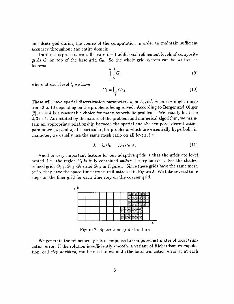
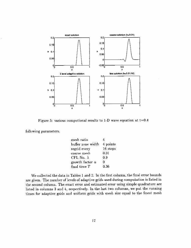
The exact solution is a wave front traveling from left to right with speed 1 and growth

rate eat, where a is a constant. Two methods are used to solve this equation: the first

order up-wind method and second-order Lax-Wendroff method. Second order Hermite

interpolation is used with both methods. In Figure 5, we plot the exact solution and

the computational solutions at t = 0.4 with a = 0 using the Lax-Wendroff method

on the coarse grid, 3-level adaptive grids with mesh ratio m = 4 and uniform grid

with mesh size equal to the smallest of the adaptive grids. Both the solutions on the

fine and 3-level adaptive grid are much better than the one on the coarse grid, which

has wiggles at the left corner where the local truncation errors are large. However,

the adaptive grid uses much less time than the uniform fine grid.Next we use the results in section 3 to control the local truncation error tolerance

6 according to the final error bound e. All the computations here are done with

16

0.2

0.15

= 0,1

0.05

o;

0.2

0.15

= 0.1

0.05

06

exact solution

0.5

x

3 level adaptive solution

0.5

x

0.2

0.15

0.1

0.05

0

-0.050

0.2

0.15

= 0.1

0.05

coarse solution (h=O.01)

0.5x

line solution (h=0.01/16)

015x

Figure 5: various computional results to 1-D wave equation at t=0.4

following parameters.

mesh ratio 4

buffer zone width 4 points

regrid every 16 stepscoarse mesh 0.01

CFL No. A 0.9

growth factor a 0final time T 0.36

We collected the data in Tables 1 and 2. In the first column, the final error bounds

are given. The number of levels of adaptive grids used during computation is listed in

the second column. The exact error and estimated error using simple quadrature are

listed in columns 3 and 4, respectively. In the last two columns, we put the running

times for adaptive grids and uniform grids with mesh size equal to the finest mesh

17

size in the corresponding adaptive grids.

Table 1

Results using the up-wind method for the 1-D wave equation

e levels exact II_hlla est. It_hll_ time time using

(sec) fine grid (sec)

5 x 10 -3 1 4.57 x 10 -3 4.54 x l0 -3 0.0 0.0

1 x 10 -3 3 9.37 x 10 -4 9.26 x 10 -4 0.4 4.7

5 x 10 -4 3 3.88 x 10 -4 3.82 x l0 -4 1.0 4.7

1 x 10 -4 4 9.98 x 10 -s 9.90 x 10 -s 12.9 77.0

Table 2

Results using the Lax-Wendroff method for the 1-D wave equation

e levels exact I1_11_ est. II_hll_ time time using

(sec) fine grid (sec)

1 x 10 -3 2 2.08 x 10 -4 1.88 × 10 -4 0.1 0.4

5 x 10 -4 2 1.86 x 10 -4 1.83 x 10 -4 0.1 0.4

1 x 10 -4 3 3.68 x 10 -5 3.81 x 10 -5 0.8 7.0

5 x 10 -s 3 2.24 x 10 -5 2.15 × 10 -5 1.0 7.0

1 x 10 -s 4 7.75 x 10 -6 7.70 x 10 -6 4.6 115.0

5 x 10 -6 4 2.68 × 10 -6 2.60 x 10 -6 10.0 115.0

Several interesting facts are illustrated in Tables 1 and 2. First of all, we see that

our adaptive strategy is very efficient for solving PDE's. It does efficiently generate

different subgrids in response to the final error tolerances. For example, when we use

Lax-Wendroff with tolerance e = 1 × 10 -3 and e = 5 x 10 -4, two levels of grids are

used in both cases. However, in order to satisfy the final error tolerance, the two

Gl's are constructed differently. This is shown in Figures 6 and 7. In the case of

e = 1 × 10 -3, two small subgrids are generated around the two corners where large

local truncation errors appear. When e is reduced to 5 × 10 -4, a large subgrid is

created in G1. The running times in Tables 1 and 2 show that the speedup, i.e., the

ratio between the time using a uniform fine mesh and the time using an adaptive

grid, increases as the final error tolerance is decreased. In other words, our adaptive

strategy is more attractive when high accuracy is needed. This is because only very

18

small regions (the two corners in this example) need to be refined. The data also

illustrate that our simple quadrature error estimation formula gives very satisfactory

results. Of cause, one reason we have such accurate estimates is that the equation has

constant coefficients. A more realistic variable coefficient problem is considered in the

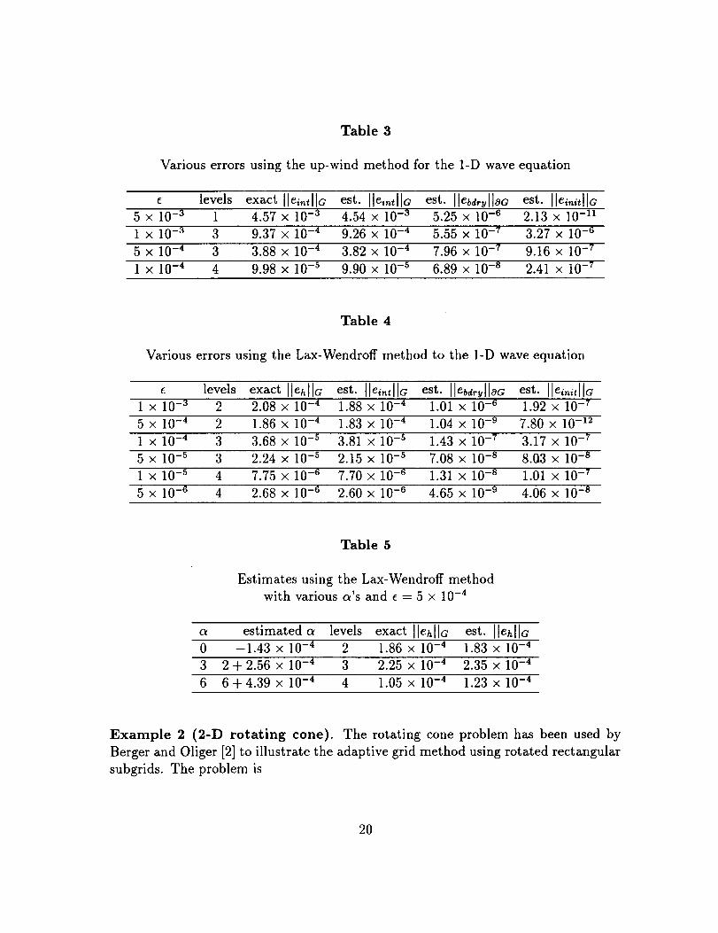
next example. As mentioned in the Section 3, the errors of interpolation and the ones

at boundaries are assumed to be relatively small compared to the local truncation

errors. Now we compute these two types of error explicitly and list them in Tables

3 and 4. To be consistent with the notation used in Section 3, we use Ile .llc to

represent the subgrids' initialization errors caused by interpolation of the coarse grids'

data. ]lei,_tlla and Ilebdrylloa are used to represent the errors caused by local trucation

errors on the interior points, and the errors on both exterior boundaries OG e=t and

interior boundaries OG i'_t, respectively. Indeed, it is shown that Ile .l la and Ilebdr lladare negligible compared to Ile ,lla. Finally we look at error estimation for different

a's, since for some nonlinear problems, the error equations contains non-differentiable

terms. The results for different a's using Lax-Wendroff with tolerance e = 0.0005 are

shown in Table 5. The estimated growth factors are listed in the table. Our error

control and estimation works very well for all three test cases, a = 0, 3 and 6.

GI,1 G1,2I--J t__l

e0,1

Figure 6: Adaptive grid structure for e = 0.001

GI,1i i

e0,1

Figure 7: Adaptive grid structure for e = 0.0005

19

Table 3

Various errors using the up-wind method for the 1-D wave equation

levels exact Ilei_tllc est. [lei_tllc est. Ilebd_yl]0C est. Ile_,,,tllc5 x 10 -3 1 4.57 x 10 -3 4.54 x 10 -3 5.25 x 10 -6 2.13 >( 10 -11

1 × 10-3 3 9.37 x 10-4 9.26 X 10 -4 5.55 × 10-7 3.27 X 10-6

5 X 10-4 3 3.88 X 10-4 3.82 X 10-4 7.96 × 10-7 9.16 X 10-7

1 X 10-4 4 9.98 X 10-5 9.90 X I0-s 6.89 X i0-s 2.41 X 10-7

Table 4

Various errors using the Lax-Wendroff method to the 1-D wave equation

levels exact Ilehlla est. lle_tllc est. Ilebd,._llOa est. Ile,,_it[la1 x 10-3 2 2.08 × 10-4 1.88 x 10-4 1.01 x 10-6 1.92 × I0-7

5 x 10-4 2 1.86 x 10-4 1.83 x 10-4 1.04 x 10-9 7.80 X 10-12

1 x 10-4 3 3.68 x I0-s 3.81 x I0-s 1.43 x 10-7 3.17 x I0-7

5 x 10-5 3 2.24 × 10-5 2.15 × I0-s 7.08 × I0-s 8.(13× I0-s

1 x 10-5 4 7.75 x 10-6 7.70 x 10-6 1.31 x I0-s 1.01 x I0-7

5 x lO-6 4 2.68 x 10-6 2.60 x lO-6 4.65 x 10-9 4.06 × I0-s

Table 5

Estimates using the Lax-Wendroff methodwith various a's and e = 5 x 10 -4

a estimated a levels exact IlehllG est. Ilehlla0 --1.43 X 10 -4 2 1.86 X 10 -4 1.83 X 10 -4

3 2+2.56X10 -4 3 2.25X10 -4 2.35X10 -4

6 6+4.39x10 -4 4 1.05x10 -4 1.23x10 -4

Example 2 (2-D rotating cone). The rotating cone problem has been used by

Berger and Oliger [2] to illustrate the adaptive grid method using rotated rectangular

subgrids. The problem is

2O

where

ut = yux- xuyS

u(x, O) =0

f(z)I.

x • [-1, 1], y • [-1,1] and t • [0,3.125]

if (x - 0.4) 2 + 1.hy 2 > 0.04

if (x - 0.4) 2 + 1.5y 2 < 0.04

f(x) = 0.25 (1 - 25((x- 0.4) 2 + y2))2.

The solution is a cone with elliptical base which rotates counterclockwise about the

origin. The solution is integrated until the cone is approximately halfway through the

first revolution. The Lax-Wendroff method and second order interpolation are used in

this example. The boundary conditions are zero inflow and first order extrapolation

at outflow. All computations are done with following parameters:

mesh ratio 4

buffer zone width 2 points

regrid every 8 stepscoarse dx 0.05

coarse dy 0.05CFL No. A 0.25

final time T 3.125

Snapshot views of the one subgrid at three intermediate time steps are shown in

Figure 8. We should mention that this example does not fully explore the power of

our stair step subgrids, since the refined regions here are elliptical, which are easily

covered by rectangular grids. We expect our stair step subgrids to be more efficient

when the geometries of subgrids are more complicated. Various computational results

are plotted in Figure 9. It shows that the solution using a coarse grid has lots of

oscillations. They are reduced dramatically if 2 levels of adaptive grids are used. If

we use 3 levels, the oscillations are invisible. Also, we see that the solutions using

adaptive grids are as good as those using uniform grids with the smallest mesh size of

the corresponding adaptive grid, which is shown by their errors (see Table 6). Next,

our error estimation developed in Section 3 is used to approximate various types of

computational errors. The results are listed in Tables 6 and 7.

Since we are solving a variable coefficient problem, the estimated IlehllO is slightly

larger than the exact one. Also, like the 1-D wave equation example, the local trun-

cation error Ilei,_tllG dominates the other two types of error, Ilebd,yl[0a and I[ei,_itlla

(see Table 7). Finally, we estimate the efficiency of our stair step subgrids. We use

21

the two levelcaseasan example. The areaof the subgrid is about 16%of the original

domain. So, the running time on this subgrid is about 167 × 16% = 26.7 (sec). Also,

we know the running time on the coarse grid is 2.7 (sec). Thus, the total time spent

on other things besides integrating the grids is about 31.7 - 26.7 - 2.7 = 2.3 (sec),

which is approximately 8% of the total time for this two level adaptive computation.

This percentage is less than that reported in [2], which was about 12% when using

rotated rectangular subgrids. Like our 1-D example, the 2-D example also shows that

the speedup increases as we decrease the final error tolerance. As mentioned earlier,

we expect our stair step subgrids to be more efficient when refined regions with more

complicated geometries are encountered.

0.8

0.6

0.4

0.2

>- 0

-0.2

-0._

-O.E

-0._

-1-1

t=3.125

I_7

1

t=1.5625

t=O

I I I I I I I I

-0.8 -0.6 -0.4 -0.2 0 0.2 0.4 0.6X

I

0.8

Figure 8: Stair step subgrids for the rotating cone problem

22

0

Y

0

Y

0

Y

exact coarse (dx=dy=O.05)

0.2-,0.1

0

-1

0 -I 0 0 -II 1 I I

x y x

2 level adaptive uniform (dx=dy=O.0125)

-1 0 -11 1 0 1 1 0

x y x

0.2"

-, 0.1.

O.

-1

3 level adaptive uniform (dx=dy=O.O03125)

-1 0 -11 1 0 1 1 0

x y x

Figure 9: Solutions for the rotating cone problem

23

Table 6

Resultsusing the Lax-Wendroffmethod for the 2-D rotating coneproblem

levels exact IJehJJa est. IJehlla time time using exact II_hllc

(sec) fine grid (sec) for fine grid1 x 10 -2 2 5.11 x 10 -3 6.70 x 10 -3 31.7 167.0 5.11 x 10 -3

1 x 10 -3 3 5.32 X 10 -4 7.40 X 10 -4 1024.0 10879.0 5.27 x 10 -4

Table 7

Various errors using the Lax-Wendroff method for the 2-D rotating cone problem

levels exact II_hlla est. It_,lla est. II_ba,_lloa est. II_.lla1 x 10 -_ 2 5.11 x 10 -z 6.70 × 10 -3 4.77 X 10 -6 1.94 × 10 -4

1 × 10-3 3 5.32 × 10-4 7.40 × 10-4 2.96 x I0-r 2.06 × 10-5

5 Conclusions

We have presented an algorithm for solving PDE's and estimating the final error

with component adaptive grid methods. Good efficiency of such grids has been illus-

trated in our 2-D example. Applying recent stability results [6] for a class of numerical

methods on uniform grids, we have proven the convergence of these methods for linear

problems on CAG's. We obtain satisfactory final error estimates. Since local trunca-

tion error estimates are obtained during the process of grid refinement, the amount

of extra work to obtain a final error estimate is very small. For linear problems, not

only can the algorithm estimate the final error, it can also be used to control the tol-

erance for the local truncation error in terms of the given final error bound. The next

challenge is to estimate errors for nonlinear problems. Although it is very hard to

establish such results for general nonlinear PDE's, Olsson and Oliger [7] have devised

a technique that makes it possible to obtain energy estimates for initial-boundary

value problems for a class of nonlinear conservation laws. The estimates for finite

difference methods on such nonlinear problems is currently under development. We

think such results will help us estimate and control errors on our CAG's for a large

class of nonlinear problems.

24

Acknowledgment

The authors wish to thank Steve Suhr for some stimulating discussion on the data

structure for the 2-D stair step grids and some figures of composite adaptive grids

used in this paper.

References

[1]

[2]

[a]

[4]

[5]

[6]

[r]

[8]

M. BERGER, Adaptive Mesh Refinement for Hyperbolic Partial Differen-

tial Equations, Ph.D. Thesis, Stanford University, Stanford, CA, 1982

(unpublished).

M. BERGER AND J. OLIGER, Adaptive Methods for Hyperbolic Partial

Differential Equations, J. Comp. Phys., 53 (1984), pp. 484-512.

B. GUSTAFSSON, H.-O. KREISS AND J. OLIGER, Time Dependent

problems and Difference Methods, 1995 (to be published by John Wiley

& Sons).

a. CHESSHIRE AND W. D. HENSHAW, Composite Overlapping Meshes

for the Solution of Partial Differential Equations, J. Comp. Phys., 90

(1990), pp. 1-64.

H. O. KREISS AND J. LORENZ, Initial-Boundary Value Problems and

the Navier-Stokes Equations, volume 136 of Pure and Applied Mathe-

matics, Academic Press, INc, San Diego, CA, 1989.

P. OLSSON, Summation by Parts, Projections and Stability, RIACS

Technical Report 93.04, RIACS, NASA Ames Research Center, Moffett

Field, CA, 1993 (unpublished).

P. OLSSON AND J. OLIGER, Energy and Maximum Norm Estimates for

Nonlinear Conservation Laws, RIACS Technical Report 94.01, RIACS,

NASA Ames Research Center, Moffett Field, CA, 1994 (unpublished).

R. G. VENKATA, J. OLIGER, AND J. H. FERZIGER, Composite Grids

for Flow Computations on Complex 3D Domains, Proc. of the Fifth

SIAM Conf. on Domain Decomp. Methods for Partial Differential Equa-

tions, (1991), pp. 605-613.

25

[9] R. G. VENKATA, Three-dimensional Composite Grid Generation using

Bezier Family of Curves and Surfaces, Second SIAM Conf. on Geom.

Design, (1991).

26