Stability in Supply Chain Networks

Michael Ostrovsky∗

Stanford GSB

September 21, 2005

Abstract

This paper presents a theory of matching in vertical networks, generalizing

the theory of matching in two-sided markets introduced by Gale and Shapley.

Under natural restrictions, stable networks are guaranteed to exist. The set of

stable networks is a lattice, with side-optimal stable networks at the extremes.

Several other key results on two-sided matching also extend naturally to the

more general setting.

∗Email address: ostrovsky@gsb.stanford.edu. I am indebted to Al Roth and Ariel Pakes for theirguidance and support throughout the project. I am also grateful to Drew Fudenberg, Parag Pathak,and Michael Schwarz for detailed and insightful comments on an earlier draft and to Attila Ambrus,John Asker, Jerry Green, Kate Ho, Paul Milgrom, Markus Mobius, Tayfun Sonmez, and Pai-LingYin for helpful comments and suggestions.

1

1 Introduction

Two-sidedness has long been viewed as a critical condition for many of the results of

matching theory, such as the existence of stable matchings and the special properties

of some of them. The original paper on stability and matching (Gale and Shapley,

1962) shows by example that the “problem of the roommates,” whose only difference

from the “marriage problem” is the absence of two sides in the market, may fail to have

a stable pairing. More generally, Abeledo and Isaak (1991) prove that to guarantee

the existence of stable pairings under arbitrary preferences, it has to be the case that

each agent belongs to one of two classes, and an agent in one class can match only with

agents in the other class. Alkan (1988) shows that the “man-woman-child marriage

problem,” in which each match consists of agents of three different types, may also fail

to have a stable matching. In their comprehensive survey of the two-sided matching

literature, Roth and Sotomayor (1990, p. 186) state:

In general, little is known about directions in which the two-sidedness of

all the models we present here can be relaxed, and which of the results

might be preserved.

In contrast, within the two-sided framework, significant progress has been made in

the last four decades both in the theoretical literature and in empirical applications.

Most recent extensions of the theoretical literature include matching with contracts,

which unifies many of the matching results with those in the literature on private

value auctions in a single framework (Hatfield and Milgrom, 2005), schedule matching,

in which agents decide not only with whom to match, but also how much time to

spend with them (Roth, Rothblum, and Vande Vate, 1993; Baiou and Balinski, 2002;

Alkan and Gale, 2003), many-to-many matching, in which agents are allowed to

match with multiple partners on the other side of the market (Echenique and Oviedo,

2

2004b), and other two-sided settings. Empirical applications include the redesign

of the matching market for American physicians (Roth, 1984a; Roth and Peranson,

1999), the design of the matching market for graduating medical students in Scotland

(Roth, 1991; Irving, 1998), the new high school admissions system in New York City

(Abdulkadiroglu, Pathak, and Roth, 2005), and several others.

This paper generalizes the results and techniques of two-sided matching to a much

broader setting—supply chain networks. Consider an industry, which includes a num-

ber of agents: workers, producers, distributors, retailers, and so on. Some agents sup-

ply basic inputs for the industry, and do not consume any of the outputs (e.g., wheat

farmers are the suppliers of basic inputs in the farmer–miller–baker–retailer supply

chain). Some agents purchase the final outputs of the industry (e.g., car manufac-

turers are the consumers of final goods in the iron ore supplier–steel producer–steel

consumer supply chain). The rest are intermediate agents, who get their inputs from

some agents in the industry, convert them into outputs at a cost, and sell the outputs

to some other agents (millers, bakers, and steel producers are intermediate agents

in the above examples). There is a pre-determined upstream-downstream partial or-

dering on the set of agents: for a pair of agents A and B, either A is a potential

supplier for B, or B is a potential supplier for A, but not both; it may also be the

case that neither is a potential supplier for the other. The partial ordering can be

complicated, with several alternative paths from one point to another, with chains of

different lengths going to the same node, and so on. However, by transitivity, it can

not have cycles. Note that if there are no intermediate agents, this setting reduces to

a two-sided market.

Agents can trade discrete quantities of goods, with the smallest tradeable quantity

(the unit of quantity) defined ex ante. For example, one unit may correspond to one

million tons of steel, one hour of work, or one loaf of bread. In the Gale-Shapley

3

two-sided marriage market, one unit corresponds to marriage, and each person can

“trade” at most one unit. Units traded in the market are represented by contracts,

following Hatfield and Milgrom (2005). Each contract specifies the buyer, the seller,

the price (if monetary transfers are involved), and the serial number of the sold unit

(if multiple units can be traded). A network is a set of contracts: it specifies who sells

what to whom and at what price. Each agent has preferences over sets of contracts

involving it: e.g., an intermediate agent’s payoff from such a set depends on the

payments it makes for its inputs (specified in its upstream contracts) and receives for

its outputs (specified in its downstream contracts), as well as on the cost of converting

the inputs into the outputs. For a consumer of final goods, the payoff depends on

the utility from the goods it purchases and the payments it makes for these goods. A

network is chain stable if there is no upstream-downstream sequence of agents (not

necessarily going all the way to the suppliers of basic inputs and the consumers of final

outputs) who could become better off by forming new contracts among themselves,

and possibly dropping some of their current contracts. This condition is parallel to

pairwise stability in two-sided markets, and is tautologically equivalent if there are

no intermediate agents in the industry.

The concept of stability in networks is not strategic—I do not study the dynamics

of network formation or “what-if” scenarios analyzed by agents who may be consid-

ering temporarily dropping or adding contracts in the hopes of affecting the entire

network in a way beneficial to them, although these considerations are undoubtedly

important in many settings. The concept is closer in spirit to general equilibrium

models, where agents perceive conditions surrounding them as given, and optimize

given those conditions. Under chain stability, agents also perceive conditions sur-

rounding them as given (i.e., which other agents are willing to form contracts with

them, and what those contracts are), and optimize given these conditions.

4

Without restrictions on preferences, the set of stable matchings may be empty

even in the two-sided one-to-many setting. One standard restriction that is sufficient

to guarantee the existence of stable matchings in that setting is the substitutes condi-

tion of Kelso and Crawford (1982). In the supply chain setting, I place an analogous

pair of restrictions on preferences; these restrictions become tautologically equiva-

lent to the substitutes condition if there are no intermediate agents in the industry.

The restrictions are same-side substitutability and cross-side complementarity. Same-

side substitutability says that when the set of available downstream contracts of a

firm expands (i.e., there are more potential customers, or the potential customers’

willingness to pay goes up), while the set of available upstream contracts remains un-

changed, the set of downstream contracts that the firm rejects also (weakly) expands,

and symmetrically, when the set of available upstream contracts expands and the set

of available downstream contracts remains unchanged, the set of rejected upstream

contracts also expands. Cross-side complementarity is a parallel restriction on how

the firm’s optimal set of downstream contracts depends on its set of available up-

stream contracts, and vice versa. It says that when the set of available downstream

contracts of a firm expands, while the set of available upstream contracts remains

unchanged, the set of upstream contracts that the firm forms also (weakly) expands,

and symmetrically, when the set of available upstream contracts expands and the set

of available downstream contracts remains unchanged, the set of downstream con-

tracts that the firm forms also expands. Section 2 gives formal definitions of these

conditions and discusses the restrictions they place on agents’ production functions

and utilities.

Section 3 states and constructively proves the main result of this paper: under

same-side substitutability and cross-side complementarity, there exists a chain stable

network. Section 4 studies properties of chain stable networks and shows that many

5

key results from the theory of two-sided matching still hold in the more general setting.

The chain stable network formed in the constructive proof of the existence theorem

is upstream-optimal: it is the most preferred chain stable network for all suppliers of

basic inputs and the least preferred chain stable network for all consumers of final

outputs. A symmetric algorithm would produce the downstream-optimal chain stable

network. In fact, just like in the two-sided setting, the set of chain stable networks is

a lattice with upstream- and downstream-optimal chain stable networks as extreme

elements. Also, adding a new supplier of basic inputs to the industry makes other such

suppliers weakly worse off and makes the consumers of final outputs weakly better off

at both upstream- and downstream-optimal chain stable networks. Symmetrically,

adding a new consumer of final outputs makes other such consumers worse off and

makes the suppliers of basic inputs better off. The section also presents results on

the equivalence of chain stability and other solution concepts: tree stability (under

same-side substitutability and cross-side complementarity) and weak core (under an

additional, very restrictive condition: each node can form at most one upstream and

at most one downstream contract). Section 5 concludes.

2 The Model of Matching in Supply Chains

This section introduces a model of matching in supply chain networks. The model

can accommodate prices, quantities, multiple traded goods, and very general network

configurations. A particular case that can be accommodated by the model, which is

perhaps the easiest to keep in mind while going through the setup and the proofs, is

a discrete analogue of a classical Walrasian equilibrium setup, with homogeneous

goods, price-taking behavior, quasilinear utilities, decreasing marginal benefits of

consumption, and increasing marginal costs of production.

6

Consider a market, consisting of a set of nodes (firms, countries, agents, workers,

etc.), A, with a partial ordering “�”, where a � b stands for b being a downstream

node for a. The interpretation of this partial ordering is that if a � b, then, in

principle, a could sell something to b, while if a 6� b and b 6� a, then there can be no

relationship between a and b. By transitivity, there are no loops in the market.

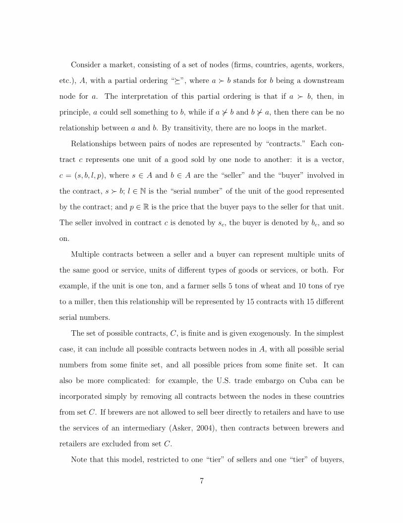
Relationships between pairs of nodes are represented by “contracts.” Each con-

tract c represents one unit of a good sold by one node to another: it is a vector,

c = (s, b, l, p), where s ∈ A and b ∈ A are the “seller” and the “buyer” involved in

the contract, s � b; l ∈ N is the “serial number” of the unit of the good represented

by the contract; and p ∈ R is the price that the buyer pays to the seller for that unit.

The seller involved in contract c is denoted by sc, the buyer is denoted by bc, and so

on.

Multiple contracts between a seller and a buyer can represent multiple units of

the same good or service, units of different types of goods or services, or both. For

example, if the unit is one ton, and a farmer sells 5 tons of wheat and 10 tons of rye

to a miller, then this relationship will be represented by 15 contracts with 15 different

serial numbers.

The set of possible contracts, C, is finite and is given exogenously. In the simplest

case, it can include all possible contracts between nodes in A, with all possible serial

numbers from some finite set, and all possible prices from some finite set. It can

also be more complicated: for example, the U.S. trade embargo on Cuba can be

incorporated simply by removing all contracts between the nodes in these countries

from set C. If brewers are not allowed to sell beer directly to retailers and have to use

the services of an intermediary (Asker, 2004), then contracts between brewers and

retailers are excluded from set C.

Note that this model, restricted to one “tier” of sellers and one “tier” of buyers,

7

encompasses various two-sided matching settings considered in the literature. Setting

l ≡ constant and p ≡ 0 turns this model into the marriage model of Gale and Shapley

(1962) if each agent is allowed to have at most one partner and the college admissions

model if agents on one side of the market are allowed to have multiple links. Setting

l ≡ constant turns it into the setup of Kelso and Crawford (1982) if agents on one

side are restricted to having at most one link and into the many-to-many matching

model of Roth (1984b, 1985) and Blair (1988) if agents on both sides are allowed to

have multiple links. Setting p ≡ 0 and assuming that all links connecting two nodes

are identical turns the model into a discrete version of the schedule matching problem

of Baiou and Balinski (2002) and Alkan and Gale (2003).

Each node can be involved in several contracts, some as a seller, some as a buyer,

but it cannot be involved in two contracts that differ only in price p, i.e., it cannot buy

or sell the same unit twice. Nodes have preferences over sets of contracts that involve

them as the buyer or the seller. For example, in the simplest case of quasilinear

utilities and profits, the utility of node a involved in a set of contracts X is

Va(X) = Wa ({(sc, bc, lc)|c ∈ X}) +∑c∈D

pc −∑c∈U

pc,

where D = {c ∈ X|a = sc} and U = {c ∈ X|a = bc}, i.e., D is the set of contracts

in X in which a is involved as a seller and U is the set of contracts in which a is

involved as a buyer. Wa(·) represents the utility from the purchased contracts for

the consumers at the downstream end of the chain, the cost of producing the sold

contracts for the suppliers at the upstream end of the chain, and the cost of converting

inputs into outputs for the intermediate nodes.

For an agent a ∈ A and a set of contracts X, let Cha(X) be a’s most preferred

(possibly empty) subset of X, let Ua(X) be the set of contracts in X in which a is

8

the buyer (i.e., upstream contracts), and let Da(X) be the set of contracts in X in

which a is the seller (i.e., downstream contracts). Subscript a will be omitted when it

is clear from the context which agent’s preferences are being considered. Preferences

are strict, i.e., function Cha(X) is single-valued. In the settings in which it is natural

to assume that several different sets of contracts should result in identical payoffs

(e.g., when two nodes can trade several identical units of a good), I assume that

ties are broken in a consistent manner, e.g., lexicographically: in the case of several

identical units of a good, that would imply that seller a prefers contract (a, b, 1, p) to

contract (a, b, 2, p), but would prefer (a, b, 2, p′) to (a, b, 1, p) for any p′ > p.

Preferences of agent a are same-side substitutable if for any two sets of con-

tracts X and Y such that D(X) = D(Y ) and U(X) ⊂ U(Y ), U(X)\U(Ch(X)) ⊂

U(Y )\U(Ch(Y )) and for any two sets X and Y such that U(X) = U(Y ) and

D(X) ⊂ D(Y ), D(X)\D(Ch(X)) ⊂ D(Y )\D(Ch(Y )). That is, preferences are

same-side substitutable if, choosing from a bigger set of contracts on one side, the

agent does not accept any contracts on that side that he rejected when he was choos-

ing from the smaller set.

Preferences of agent a are cross-side complementary if for any two sets of contracts

X and Y such that D(X) = D(Y ) and U(X) ⊂ U(Y ), D(Ch(X)) ⊂ D(Ch(Y )) and

for any two sets X and Y such that D(X) ⊂ D(Y ) and U(X) = U(Y ), U(Ch(X)) ⊂

U(Ch(Y )). That is, preferences are cross-side complementary if, when presented with

a bigger set of contracts on one side, an agent does not reject any contract on the

other side that he accepted before.

Same-side substitutability is a generalization of the gross substitutes condition

introduced by Kelso and Crawford (1982) and used widely in the matching literature.

If there are only two sides in the supply chain market, then these two conditions

become tautologically equivalent. Cross-side complementarity can be viewed as a

9

mirror image of same-side substitutability. It is automatically satisfied in any two-

sided market.

It is important to highlight what is allowed and what is not allowed by this pair of

assumptions. Two possibilities that they rule out are scale economies and production

functions with fixed costs, because in those cases a firm may decide not to produce one

unit of a good at a certain price, while being willing to produce ten units at the same

price, violating same-side substitutability. In addition, complementary inputs (or out-

puts) are ruled out. In contrast, with substitutable inputs and outputs and decreasing

returns to scale, many production and utility functions can be accommodated. The

simplest example is a firm that can take one kind of input and produce one kind of

output at a cost, with the marginal cost of production increasing or staying constant

in quantity. The input good can come from several different nodes, and the output

good may go to several different nodes, with different transportation costs. Much

more general cases are possible as well: preferences and production functions with

quotas and tariffs, several different inputs and outputs with discrete choice demands

and production functions, capacity constraints and increasing transportation costs,

etc. The interdependencies between different inputs or outputs can be rather complex

as well. Consider the following example. A firm has two plants in the same location.

Each plant’s capacity is equal to one unit. The first plant can convert one unit of

iron ore into one unit of steel for c1o or it can convert one unit of steel scrap into one

unit of steel for c1s. The second plant can convert one unit of iron ore into one unit of

steel for c2o or it can convert one unit of steel scrap into one unit of steel for c2

s. Then,

for a generic choice of costs and prices, the preferences of this firm will be same-side

substitutable and cross-side complementary, even though the firm’s preferences over

iron ore and scrap are not trivial (they cannot be expressed by simply saying that two

alternative inputs are perfect substitutes, with one being better than the other by a

10

certain amount x). This example is an analogue of “endowed assignment valuations”

in two-sided matching markets, introduced by Hatfield and Milgrom (2005), in which

each firm has several unit-capacity jobs, each worker has a certain productivity at

each job, and each firm has an initial endowment of workers. Even in the two-sided

setting, it is an open question whether endowed assignment valuations exhaust the

set of utility functions with substitutable preferences, and so it is an open question

in the supply chain setting as well. For the remainder of this paper, all preferences

are assumed to be same-side substitutable and cross-side complementary, and these

restrictions will usually be omitted from the statements of results to avoid repetition.

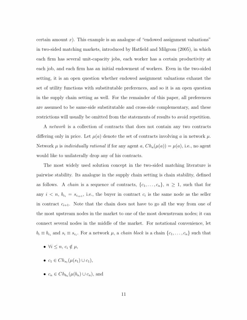
A network is a collection of contracts that does not contain any two contracts

differing only in price. Let µ(a) denote the set of contracts involving a in network µ.

Network µ is individually rational if for any agent a, Cha(µ(a)) = µ(a), i.e., no agent

would like to unilaterally drop any of his contracts.

The most widely used solution concept in the two-sided matching literature is

pairwise stability. Its analogue in the supply chain setting is chain stability, defined

as follows. A chain is a sequence of contracts, {c1, . . . , cn}, n ≥ 1, such that for

any i < n, bci= sci+1

, i.e., the buyer in contract ci is the same node as the seller

in contract ci+1. Note that the chain does not have to go all the way from one of

the most upstream nodes in the market to one of the most downstream nodes; it can

connect several nodes in the middle of the market. For notational convenience, let

bi ≡ bciand si ≡ sci

. For a network µ, a chain block is a chain {c1, . . . , cn} such that

• ∀i ≤ n, ci /∈ µ,

• c1 ∈ Chs1(µ(s1) ∪ c1),

• cn ∈ Chbn(µ(bn) ∪ cn), and

11

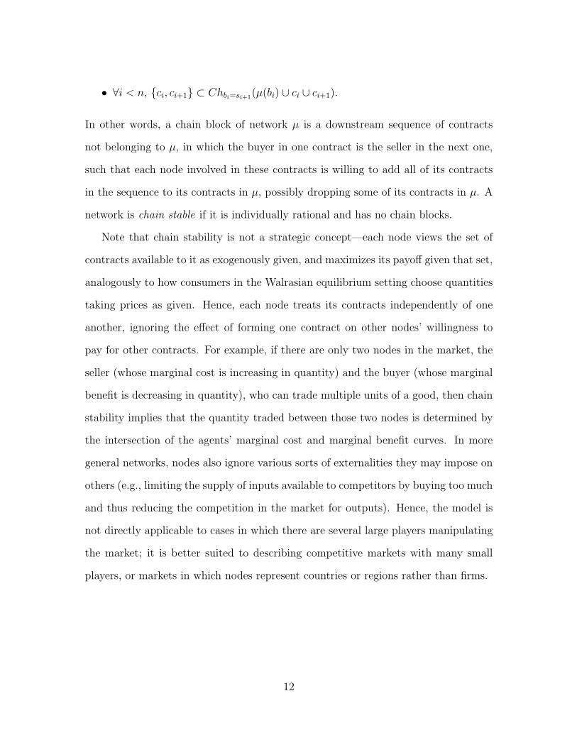
• ∀i < n, {ci, ci+1} ⊂ Chbi=si+1(µ(bi) ∪ ci ∪ ci+1).

In other words, a chain block of network µ is a downstream sequence of contracts

not belonging to µ, in which the buyer in one contract is the seller in the next one,

such that each node involved in these contracts is willing to add all of its contracts

in the sequence to its contracts in µ, possibly dropping some of its contracts in µ. A

network is chain stable if it is individually rational and has no chain blocks.

Note that chain stability is not a strategic concept—each node views the set of

contracts available to it as exogenously given, and maximizes its payoff given that set,

analogously to how consumers in the Walrasian equilibrium setting choose quantities

taking prices as given. Hence, each node treats its contracts independently of one

another, ignoring the effect of forming one contract on other nodes’ willingness to

pay for other contracts. For example, if there are only two nodes in the market, the

seller (whose marginal cost is increasing in quantity) and the buyer (whose marginal

benefit is decreasing in quantity), who can trade multiple units of a good, then chain

stability implies that the quantity traded between those two nodes is determined by

the intersection of the agents’ marginal cost and marginal benefit curves. In more

general networks, nodes also ignore various sorts of externalities they may impose on

others (e.g., limiting the supply of inputs available to competitors by buying too much

and thus reducing the competition in the market for outputs). Hence, the model is

not directly applicable to cases in which there are several large players manipulating

the market; it is better suited to describing competitive markets with many small

players, or markets in which nodes represent countries or regions rather than firms.

12

3 Stable Networks: Existence

This section shows that the set of chain stable networks is isomorphic to the non-

empty set of fixed points of a certain isotone operator, and presents a family of

algorithms for finding two special stable networks. These algorithms generalize the

fixed-point algorithms of Adachi (2000), Echenique and Oviedo (2004a, 2004b), and

Hatfield and Milgrom (2005), all of which are descendants of the Deferred Acceptance

Algorithm (Gale and Shapley, 1962) and apply only to two-sided matching problems.

Let me first introduce some definitions and notation.

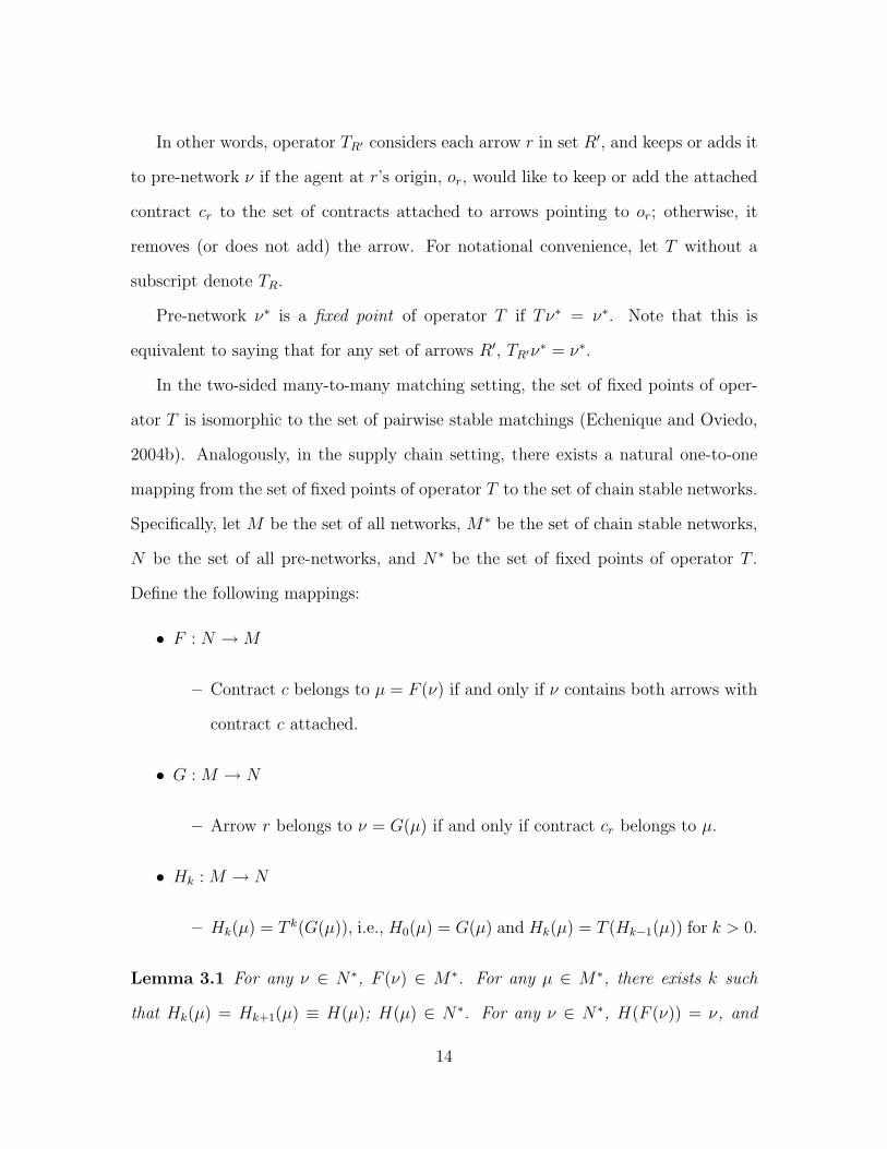
A pre-network is a set of arrows from nodes in A to other nodes in A, with the

following properties. Each arrow r is a tuple (or, dr, cr), where or (“origin of arrow r”)

and dr (“destination of arrow r”) are two different nodes and cr (“contract attached

to arrow r”) is a contract involving both or and dr. If or is the seller and dr is

the buyer of contract cr, the arrow is “downstream”. Otherwise, or is the buyer

and dr is the seller of contract cr, and the arrow is “upstream”. For a pre-network

ν and a node a, ν(a) is the set of contracts attached to arrows pointing to a, i.e.,

ν(a) = {r ∈ ν|dr = a}.

There can be multiple arrows going from or to dr, but any two arrows going from

or to dr must have different contracts attached to them (these contracts may differ

in serial numbers, prices, or both). Arrows going in opposite directions (from node a

to node b and from node b to node a) can have identical contracts attached to them.

Let R be the set of all possible arrows, and let R′ ⊂ R be an arbitrary set of

arrows. Let ν be a pre-network. Define operator TR′ on the set of pre-networks as

TR′(ν) = (ν\R′) ∪ {r ∈ R′|cr ∈ Chor (ν(or) ∪ cr)}.

13

In other words, operator TR′ considers each arrow r in set R′, and keeps or adds it

to pre-network ν if the agent at r’s origin, or, would like to keep or add the attached

contract cr to the set of contracts attached to arrows pointing to or; otherwise, it

removes (or does not add) the arrow. For notational convenience, let T without a

subscript denote TR.

Pre-network ν∗ is a fixed point of operator T if Tν∗ = ν∗. Note that this is

equivalent to saying that for any set of arrows R′, TR′ν∗ = ν∗.

In the two-sided many-to-many matching setting, the set of fixed points of oper-

ator T is isomorphic to the set of pairwise stable matchings (Echenique and Oviedo,

2004b). Analogously, in the supply chain setting, there exists a natural one-to-one

mapping from the set of fixed points of operator T to the set of chain stable networks.

Specifically, let M be the set of all networks, M∗ be the set of chain stable networks,

N be the set of all pre-networks, and N∗ be the set of fixed points of operator T .

Define the following mappings:

• F : N → M

– Contract c belongs to µ = F (ν) if and only if ν contains both arrows with

contract c attached.

• G : M → N

– Arrow r belongs to ν = G(µ) if and only if contract cr belongs to µ.

• Hk : M → N

– Hk(µ) = T k(G(µ)), i.e., H0(µ) = G(µ) and Hk(µ) = T (Hk−1(µ)) for k > 0.

Lemma 3.1 For any ν ∈ N∗, F (ν) ∈ M∗. For any µ ∈ M∗, there exists k such

that Hk(µ) = Hk+1(µ) ≡ H(µ); H(µ) ∈ N∗. For any ν ∈ N∗, H(F (ν)) = ν, and

14

for any µ ∈ M∗, F (H(µ)) = µ. In other words, removing one-directional links from

any fixed-point pre-network results in the corresponding chain stable network, and

iterating operator T starting with a chain stable network results in the corresponding

fixed-point pre-network.

Proof. See Appendix.

To demonstrate the existence of chain stable networks, it is now sufficient to prove

that operator T has a fixed point. To do that, I introduce a partial ordering on the

set of pre-networks. Let ν1 and ν2 be two pre-networks. Then ν1 ≤ ν2 if the set

of downstream arrows in ν1 is a subset of the set of downstream arrows in ν2, and

the set of upstream arrows in ν1 is a superset of the set of upstream arrows in ν2.

Also, let νmin be the pre-network that includes all possible upstream arrows and

no downstream arrows, and let νmax be the pre-network that includes no upstream

arrows and all possible downstream arrows. By construction, for any pre-network ν,

νmin ≤ ν ≤ νmax.

Let R1, R2, . . . , Rk be an arbitrary sequence of sets of arrows. Let ν0 = νmin, and

let νi = TRi(νi−1) for i > 0.

Lemma 3.2 For any i < k, νi ≤ νi+1.

Proof. See Appendix.

For a given pre-network ν0, call a sequence of sets of arrows regular if it satisfies

the following condition: for i ≥ 1, if νi ≡ TRiνi−1 = νi−1 and Ri 6= R, then Ri+1 % Ri.

In particular, the sequence Ri ≡ R is regular.

Theorem 3.1 There exists a chain stable network.

Proof. Fix ν0 = νmin and take any infinite regular sequence of sets of arrows. By

Lemma 3.2, the corresponding sequence of pre-networks is monotonically increasing.

15

The set of pre-networks is finite, and therefore this sequence of pre-networks con-

verges, in finite time, to a fixed point, ν∗; TR′ν∗ = ν∗ for any set of arrows R′. By

Lemma 3.1, F (ν∗) is a chain stable network.

Note that the proof of Theorem 3.1 is constructive: it gives an algorithm for

computing a chain stable network. In fact, it produces a family of such algorithms:

a different algorithm for each regular sequence of sets. It turns out that all these

algorithms generate the same fixed point of operator T , and therefore the same chain

stable network. To show that, I first state an auxiliary lemma. Its proof is completely

analogous to the proof of Lemma 3.2, and is therefore omitted.

Lemma 3.3 For any set of arrows R′ and any pre-networks ν1 ≤ ν2, TR′(ν1) ≤

TR′(ν2).

Theorem 3.2 Let ν0 = νmin. Then for all regular sequences of sets of arrows, the

corresponding sequences of pre-networks converge to the same fixed point ν∗min.

Proof. Consider any two regular sequences of sets of arrows {R11, R

12, . . . } and

{R21, R

22, . . . } and corresponding fixed points ν1 and ν2. Now,

ν1 ≥ νmin = ν20

TR21(ν1) = ν1 ≥ TR2

1(νmin) = ν2

1

TR22(TR2

1(ν1)) = ν1 ≥ TR2

2(TR2

1(νmin)) = ν2

2

...

ν1 ≥ ν2k .

Since ν2k converges to ν2, we know that ν1 ≥ ν2. Symmetrically, ν2 ≥ ν1, and so

ν1 = ν2.

16

Therefore, it does not matter in what order various parts of the pre-network are

updated—the outcome will be the same. This flexibility may simplify and speed up

computational implementations of the algorithm. This family of algorithms also corre-

sponds to various two-sided matching algorithms in a natural way. The T -algorithm

of Adachi (2000) and Echenique and Oviedo (2004a, b) and the generalized Gale-

Shapley algorithm of Hatfield and Milgrom (2005) are equivalent to my algorithm

with Rk ≡ R. Men-proposing deferred acceptance algorithm of Gale and Shapley

(1962) is equivalent to my algorithm with ν0 containing all arrows from women to

men and no arrows from men to women, Rk containing all arrows from men to women

when k is odd, and Rk containing all arrows from women to men when k is even.

Note also that all proofs would remain essentially unchanged if ν0 was set equal to

νmax rather than νmin everywhere. The algorithms would then converge to a possibly

different fixed point, ν∗max. The next section explores the properties of the set of fixed

points of operator T , and the special role that ν∗min and ν∗max play in this set.

4 Stable Networks: Properties

This section discusses several properties of the set of chain stable networks (lattice

structure, side optimality, and comparative statics) and connections between chain

stability and other solution concepts (tree stability and the core).

4.1 Lattice Structure and Comparative Statics

The first result shows that ν∗min and ν∗max are the extreme fixed points of operator T ,

and that the set of fixed points of operator T is a lattice. This is a generalization

of similar results for matching with contracts (Hatfield and Milgrom, 2005), many-

to-many matching (Echenique and Oviedo, 2004b), schedule matching (Alkan and

17

Gale, 2003), and other two-sided matching settings. This result is a corollary of

Tarski’s fixed point theorem for isotone operators on lattices, but I also give a simple

alternative proof for completeness.

Theorem 4.1 The set of fixed points of operator T is a lattice with extreme elements

ν∗min and ν∗max.

Proof. See Appendix.

Now, let A = {a ∈ A : Ua(A) = ∅} and A = {a ∈ A : Da(A) = ∅}, i.e., A and A

are the sets of suppliers of initial inputs for the market (“suppliers”) and consumers

of final outputs (“consumers”), respectively. In the two-sided matching setup, one

side of the market is A and the other side is A; in more general networks, there is

also a set of “intermediate” points, A\(A ∪ A).

The following theorem generalizes another standard result from the two-sided

matching literature, which says that the extreme elements of the lattice of stable

matchings are side-optimal (Gale and Shapley, 1962).

Theorem 4.2 Let µmin = F (ν∗min), µmax = F (ν∗max), and let µ be a chain stable

network. Then any a ∈ A (weakly) prefers µmin to µ and µ to µmax, and any a ∈ A

(weakly) prefers µmax to µ and µ to µmin.

Proof. See Appendix.

Note that the theorem does not say anything about intermediate nodes. In fact,

one can construct examples to show that an intermediate agent’s most preferred chain

stable network may be neither µmin nor µmax and, moreover, different intermediate

agents may have different most preferred chain stable networks.

Finally, in two-sided one-to-many matching markets, adding a worker makes other

workers (weakly) worse off at the firm- and worker-optimal stable matchings, and

18

makes firms (weakly) better off; symmetrically, the opposite is true when a firm is

added to the market (Kelso and Crawford, 1982; Gale and Sotomayor, 1985). The

following theorem extends this result to the supply chain setting.

Theorem 4.3 Let A′ = A ∪ a′, where Ua′(A) = ∅, and preferences of all nodes in

the larger market remain same-side substitutable and cross-side complementary. Let

µ′min and µ′

max be the smallest and the largest chain stable matchings in A′. Then

each a ∈ A is at least as well off in µmax as in µ′max, and at least as well off in µmin

as in µ′min; each a ∈ A is at most as well off in µmax as in µ′

max, and at most as

well off in µmin as in µ′min. The opposite is true if a′ is added to the other end of the

market, i.e., Da′(A) = ∅.

Proof. See Appendix.

Again, the change in the welfare of intermediate agents is ambiguous—it can go

either way. Adding new intermediate nodes can also have opposite effects on different

extreme nodes (e.g., some a ∈ A may become better off, while others may become

worse off), as well as on other intermediate nodes.

4.2 Chain Stability, Tree Stability, and the Core

In two-sided one-to-one matching markets, the set of pairwise stable matchings co-

incides with the core. In more general models, this is no longer true, even when

preferences are substitutable: in one-to-many matching markets, the set of pairwise

stable matchings is equal to the weak core but not to the strict core, and in many-

to-many matching markets, even that result no longer holds. Nevertheless, pairwise

stability is a natural solution concept even in many-to-many matching markets, since,

as Roth and Sotomayor (1990, p. 156) argue, “identifying and organizing large coali-

tions may be more difficult than making private arrangements between two parties,

19

and the experience of those regional [many-to-many matching] markets in the United

Kingdom that are built around stable mechanisms suggests that pairwise stability is

still of primary importance in these markets.”

Since the model of this paper nests two-sided many-to-many matching models,

different solution concepts can result in different predictions. However, just like pair-

wise stability in the two-sided setting, chain stability is a natural solution concept

in the supply chain environment. The reason for that is that chain blocks are par-

ticularly easy to identify and organize: A customer just needs to pick up the phone

and call a potential supplier asking him whether he would like to form a contract;

the potential supplier, after receiving that phone call, in turn calls one of his poten-

tial suppliers, and so on. If there is a chain block, it can be easily identified in this

way, and subsequently the contracts can be formed. In contrast, larger coalitions

require much more coordination and information exchange between the agents, and

may even violate antitrust laws if they require communication between competing

firms. Of course, the similarity between the arguments behind pairwise stability in

the two-sided case and chain stability in the more general case is not a coincidence:

Chain stability reduces to pairwise stability if there are no intermediate agents.

Still, it is important to understand the differences and similarities between various

solution concepts in matching markets. Several papers address these issues in two-

sided markets (see, e.g., the recent papers by Echenique and Oviedo, 2004b, and

Konishi and Unver, 2005, and references in those papers). The following two results

provide a starting point for the analysis of the relationship between chain stability

and other solution concepts in supply chain networks.

The first result shows that under same-side substitutability and cross-side com-

plementarity, blocking by “trees” is equivalent to blocking by chains. More formally,

a sequence of contracts c1, . . . , ci is a path from node a to node b if: (i) node a is

20

involved in contract c1 and not involved in any contract cj for j > 1; (ii) node b is

involved in contract ci and not involved in any contract cj for j < i; and (iii) any

other node x involved in one of the contracts cj for 1 ≤ j ≤ i is involved in exactly

two such contracts, and these two contracts are adjacent in the sequence (i.e., if one

of the contracts is ck, then the other is either ck−1 or ck+1). Note that while each

chain is a path, there are paths that are not chains: e.g., a pair of contracts with the

same buyer and two different sellers is a path connecting the two sellers, but is not

a chain. A tree is a set of contracts such that for any two nodes involved in these

contracts, there exists exactly one path in this set connecting the two nodes. Note

that every chain is a tree. A network, µ, is blocked by a tree, τ , if τ ∩ µ = ∅ and for

every node a involved in τ , τ(a) ⊂ Cha(µ(a) ∪ τ(a)). A network is tree stable if it is

not blocked by any tree.

Theorem 4.4 Under same-side substitutability and cross-side complementarity, the

set of tree stable networks is equal to the set of chain stable networks.

Proof. See Appendix.

The final result of this section shows that in a special case, in which each node

is restricted to having at most one upstream contract and at most one downstream

contract, the set of chain stable networks coincides with the weak core of the matching

game. Network µ is in the weak core of the matching game if and only if there is no

other network µ′ and set M of nodes such that (i) for every node a ∈ M , for every

contract c involving a, the other node involved in c is also in set M ; (ii) every node

a ∈ M weakly prefers the set of contracts in which it is involved in µ′ to the set of

contracts in which it is involved in µ; and (iii) at least one node a ∈ M strictly prefers

the set of contracts in which it is involved in µ′ to the set of contracts in which it is

involved in µ.

21

Theorem 4.5 If each node a ∈ A can have at most one upstream contract and at

most one downstream contract, and preferences are same-side substitutable and cross-

side complementary, then the set of chain stable networks is equal to the weak core of

the matching game.

Proof. See Appendix.

5 Conclusion

This paper shows that two-sidedness is not a necessary condition for many key results

of matching theory. Under same-side substitutability and cross-side complementarity,

chain stable networks are guaranteed to exist. The set of chain stable networks is a

lattice with two extreme elements: the optimal chain stable network for the suppliers

of basic inputs, and the optimal chain stable network for the consumers of final

outputs. Adding a supplier of basic inputs makes other suppliers weakly worse off at

the side-optimal stable networks, and makes the consumers of final outputs weakly

better off; adding a consumer of final outputs has the opposite effect.

There are several open questions and promising directions for future work related

to the theory of matching in supply chains. One of them is figuring out how to model

strategic interactions in this setting. With one strategic player, this is straightforward:

the strategic player simply chooses the contracts that maximize his payoff, given the

non-strategic behavior of the rest of the market. With more than one player, however,

it is hard to model strategic behavior even in two-sided markets, and so it is unclear

how to do it in the broader supply chain setting.

Another important question is whether cross-side complementarity or same-side

substitutability restrictions can be partially relaxed, while preserving some of the

properties of the model. In general, same-side complementarities present difficulties

22

for the analysis of matching markets. However, it is possible that in some cases,

complementary inputs or economies of scale can be incorporated into the standard

models. For example, if a two-sided market includes one type of buyers ({x1, x2, . . . })

and two types of sellers ({y1, y2, . . . } and {z1, z2, . . . }), so that the buyers are sub-

stitutes (from the point of view of the sellers), the sellers of the same type are also

substitutes (from the point of view of the buyers), and the sellers of different types are

complements (also from the point of view of the buyers), then stable matchings are

guaranteed to exist (because this matching market can be viewed as the Y � X � Z

“supply chain market”).

Finally, the model readily lends itself to empirical applications. In Ostrovsky

(2005) it is used to incorporate heterogeneity of bilateral transportation costs into

a model of international trade flows in the steel supply chain. Unlike conventional

continuous equilibrium models that incorporate heterogeneity, this framework does

not rely on any specific functional form assumptions and can accommodate arbitrary

distributions of transportation costs, production functions, and utilities. There may

be other interesting settings to which the theory can be applied. For instance, con-

tracts in the model can specify different times at which goods can be shipped, making

it possible to analyze various intertemporal settings in the matching framework. Fur-

ther extending the theoretical model of matching in supply chains and using it to

answer new empirical questions are likely to be exciting areas for future research.

23

Appendix

Proof of Lemma 3.1

Step 1. Let us show that for any pre-network ν such that Tν = ν, µ = F (ν) is a

chain stable network.

First, we need to make sure that µ is indeed a network, i.e., there are no contracts

in µ that differ only in price. To see this, note that if there are two contracts that differ

only in price in µ, that implies that each of the two agents involved in these contracts

would choose both contracts when selecting from some larger set containing them.

But this is impossible, because each agent, by definition, chooses only one contract

with a given partner and a particular serial number—the one with the most favorable

price.

Second, we need to show that network µ is individually rational. To see that, note

that for any agent a, µ(a) = Cha(ν(a)), and so a does not want to drop any of its

contract in µ (because that would imply that µ(a) 6= Cha(µ(a)) = Cha(Cha(ν(a))) =

Cha(ν(a)) = µ(a)).

Finally, we need to show that there are no chain blocks. Suppose (c1, c2, . . . , cn) is a

chain block of µ, and let si and bi denote the seller and the buyer involved in contract i.

Since c1 ∈ Chs1(µ(s1)∪c1), it has to be the case that c1 ∈ Chs1(ν(s1)∪c1) (otherwise,

Chs1(ν(s1)∪c1) = Chs1(ν(s1)) = µ(s1), and hence no subset of µ(s1)∪c1 ⊂ ν(s1)∪c1

can be better for s1 than µ(s1)), and so the arrow r1 from s1 to b1 with c1 attached

must be in Tν = ν. Now, by assumption, s2 would like to sign contracts c1 and c2, i.e.,

{c1, c2} ⊂ Chs2(µ(s2)∪ c1 ∪ c2). If neither c1 nor c2 are in Chs2(ν(s2)∪ c1 ∪ c2), then

Chs2(ν(s2) ∪ c1 ∪ c2) = Chs2(ν(s2)) = µ(s2), and so {c1, c2} 6⊂ Chs2(µ(s2) ∪ c1 ∪ c2),

which would contradict our assumptions. Suppose c2 /∈ Chs2(ν(s2) ∪ c1 ∪ c2). Then

c1 ∈ Chs2(ν(s2)∪c1∪c2) = Chs2(ν(s2)∪c1), and so there must be an arrow from s2 to

24

s1 with contract c1 attached in Tν = ν, which together with the fact that there is an

arrow from s1 to s2 with c1 attached in ν would imply that c1 ∈ µ, which would also

contradict our assumptions. Hence, it must be the case that c2 ∈ Chs2(ν(s2)∪c1∪c2).

Proceeding by induction, there is an arrow from si to si+1 with ci attached in ν for

any i < n. Similarly, we could have started from node bn, and so there must be an

arrow going from bn to bn−1 = sn with cn attached in ν, which implies that cn ∈ µ—

contradiction. Therefore, for any ν = Tν, F (ν) is a chain stable network.

Step 2. Let us now show that for any chain stable network µ, for some n,

Hn(µ) = Hn+1(µ) and moreover, F (Hn(µ)) = µ. For convenience, let νn = Hn(µ),

ν0 = G(µ). We will show by induction on k that: (i) F (νk) = µ and (ii) νk ⊃ νk−1.

For k = 1, (ii) follows from the individual rationality of µ and (i) follows from the

absence of chain blocks of length 1 (i.e., pairwise blocks) of µ. Suppose (i) and (ii)

hold up to k − 1. Let us show that they hold for k.

(i) Suppose arrows r and r′ with contract cr attached are in νk, but cr /∈ µ. We

will now “grow” a chain block of µ from this contract cr.

Consider arrow r first; without loss of generality, assume it is upstream. Let c0 =

cr and r0 = r. If cr ∈ Chor(µ(or) ∪ cr), stop. Otherwise, since cr ∈ Chor(νk−1(or) ∪

cr), by same-side substitutability cr ∈ Chor(Dor(νk−1(or)) ∪ Uor(µ(or)) ∪ cr). Let

x1, x2, . . . , xm be the contracts in Dor(νk−1(or))\Dor(µ(or)). Then for some j, xj ∈

Chor(µ(or) ∪ xj ∪ cr) (otherwise, by same-side substitutability, for any j, xj /∈

Chor(µ(or) ∪ cr ∪ x1 ∪ x2 ∪ · · · ∪ xm), which is then equal to Chor(µ(or) ∪ cr), which

contradicts our assumption that cr /∈ Chor(µ(or) ∪ cr)). It must also be the case

that cr ∈ Chor(µ(or) ∪ xj ∪ cr), because otherwise xj ∈ Chor(µ(or) ∪ xj) and so

the downstream arrow with xj attached is in ν1, and is therefore in νk−1 (by state-

ment (ii) in the step of induction, ν1 ⊂ νk−1). But then both arrows with xj at-

tached are in νk−1, which contradicts assumption (i) of induction for k − 1. Hence,

25

{cr, xj} ⊂ Chor(µ(or) ∪ xj ∪ cr).

Let c1 = xj. By construction, the upstream arrow r1 with c1 attached is in νk−1,

but c1 /∈ µ. Let o1 denote the origin of arrow r1. If c1 ∈ Cho1(µ(o1) ∪ c1), stop;

otherwise, following the procedure above, generate c2 ∈ Do1(νk−2(o1))\Do1(µ(o1)),

and so on. At some point, this procedure will have to stop (since we keep going

downstream). Now, “grow” cr in the other direction, starting with arrow r′. We end

up with a chain cx, cx+1, . . . , c0, . . . , cy−1, cy, which, by construction, is a chain block

of µ—contradiction.

(ii) Suppose some upstream arrow r is in νk−1, but not in νk, i.e., cr ∈ Chor(νk−2(or)∪

cr), but cr /∈ Chor(νk−1(or) ∪ cr). Then by (i), Chor(ν

k−1(or) ∪ cr) = µ(or) =

Chor(Dor(νk−1(or))∪Uor(µ(or))∪cr). From cr /∈ Chor(Dor(ν

k−1(or))∪Uor(µ(or))∪cr),

by same-side substitutability and by assumptions of induction for k − 2, we get

cr /∈ Chor(Dor(νk−1(or)) ∪ Uor(ν

k−2(or)) ∪ cr), and from that, by cross-side com-

plementarity and assumption (ii) of induction for k − 1 (i.e., νk−2 ⊂ νk−1), we get

cr /∈ Chor(Dor(νk−2(or))∪Uor(ν

k−2(or))∪ cr) = Chor(νk−2(or)∪ cr), and so r is not in

νk−1—contradiction. The proof for a downstream arrow r′ is completely analogous.

This completes the proof of statements (i) and (ii) of induction.

Now, since G(µ) ⊂ H1(µ) ⊂ H2(µ) ⊂ . . . is an increasing sequence and the set

of possible arrows is finite, this sequence has to converge, i.e., for some n, Hn(µ) =

Hn+1(µ) = H(µ). By (ii), all arrows in G(µ) are also present in H(µ), and by (i),

any pair of arrows with the same contract attached in H(µ) is also present in G(µ).

Therefore, F (H(µ)) = µ.

Finally, we need to show that for two fixed points of operator T , ν∗1 and ν∗2 ,

F (ν∗1) 6= F (ν∗2). Suppose ν∗1 6= ν∗2 and F (ν∗1) = F (ν∗2) = µ. Consider the set of agents

for whom the upstream arrows originating from them are not the same in ν∗1 and

ν∗2 . Take one of the “most downstream” agents in this set (i.e., such an agent o that

26

there is nobody downstream from him in this set), and take an upstream arrow r

originating from o such that it is in only one of the two pre-networks. Without loss of

generality, r ∈ ν∗1 and r /∈ ν∗2 . r /∈ ν∗2 ⇒ cr /∈ Cho(ν∗2(o) ∪ cr) = Cho(ν

∗2(o)) = µ(o) =

Cho(Do(ν∗2(o))∪Uo(µ(o))∪ cr). By the assumption that o is the “most downstream”

agent whose upstream arrows differ in the two pre-networks, Do(ν∗2(o)) = Do(ν

∗1(o)),

and hence cr /∈ Cho(Do(ν∗1(o)) ∪ Uo(µ(o)) ∪ cr). Now, since F (ν∗1) = µ, Uo(ν

∗1(o)) ⊃

Uo(µ(o)), and so by same-side substitutability, cr /∈ Cho(Do(ν∗1(o))∪Uo(ν

∗1(o))∪cr) =

Cho(ν∗1(o) ∪ cr), and therefore r /∈ ν∗1—contradiction.

Proof of Lemma 3.2

By induction on i. For i = 0, the statement is true by construction. Consider some i

such that the statement is true for 0, . . . , i−1. We need to check that all downstream

arrows in νi belong to νi+1, and that all upstream arrows in νi+1 belong to νi. Since

only arrows belonging to Ri+1 are affected by operator TRi+1, we can restrict our

attention to them.

Consider a downstream arrow r in νi∩Ri+1. Since there are no downstream arrows

in ν0, there must be at least one t such that r ∈ Rt. Let j = max{0<t<i+1}{t|r ∈ Rt}.

Since r ∈ νi and j was the last time this arrow was updated, r must belong to νj,

and so cr ∈ Chor(νt−1(or) ∪ cr). By induction and transitivity, νj−1 ≤ νi, and so

U(νj−1(or)) ⊂ U(νi(or)) (i.e., the set of arrows pointing to or from upstream nodes

is smaller in νj−1 than it is in νi) and D(νj−1(or)) ⊃ D(νi(or)). Thus, (D(νj−1(or))∪

cr) ⊃ (D(νi(or)) ∪ cr), and by same-side substitutability, cr ∈ Chor((D(νi(or)) ∪

cr) ∪ U(νj−1(or))). Now, by cross-side complementarity, cr ∈ Chor((D(νi(or)) ∪ cr) ∪

U(νi(or))), i.e., cr ∈ Chor(νi(or) ∪ cr), and so r ∈ νi+1.

For upstream arrows, the argument is completely symmetric: if an upstream arrow

27

r′ ∈ Ri+1 is not in νi, consider the last time j this arrow was updated, and then show

by same-side substitutability and cross-side complementarity that this arrow is not

in νi+1.

Proof of Theorem 4.1

Take any two fixed points of operator T , ν∗1 and ν∗2 . Let ν12 be the least upper bound of

these two pre-networks in the original lattice. ν12 ≥ ν∗1 , ν12 ≥ ν∗2 ⇒ Tν12 ≥ Tν∗1 = ν∗1 ,

Tν12 ≥ Tν∗2 = ν∗2 ⇒ Tν12 ≥ ν12, and so for some n, ν12 ≤ Tν12 ≤ T 2ν12 ≤ · · · ≤

T nν12 = T n+1ν12 = ν∗12. By construction, ν∗12 ≥ ν∗1 and ν∗12 ≥ ν∗2 . To see that any

other upper bound of ν∗1 and ν∗2 (say, ν∗3) has to be greater than ν∗12, note that ν∗3 ≥ ν∗1 ,

ν∗3 ≥ ν∗2 implies ν∗3 ≥ ν12 ⇒ Tν∗3 = ν∗3 ≥ Tν12 ⇒ · · · ⇒ ν∗3 ≥ ν∗12. The greatest lower

bound of ν∗1 and ν∗2 can be constructed in an analogous way.

To show that ν∗min is the lowest fixed point, consider another fixed point ν∗, and

note that ν∗ ≥ νmin ⇒ Tν∗ = ν∗ ≥ Tνmin ⇒ · · · ⇒ ν∗ ≥ ν∗min. Analogously, ν∗max is

the highest fixed point of operator T .

Proof of Theorem 4.2

Let ν = H(µ). Since ν∗min and ν∗max are the extreme fixed points of operator T ,

ν∗min ≤ ν ≤ ν∗max. Take any a ∈ A (the proof for the symmetric case a ∈ A is

completely analogous). By definition of A, a can only be connected with downstream

nodes. Therefore, the set of arrows pointing to a in ν∗min is a superset of arrows

pointing to a in ν, which in turn is a superset of arrows pointing to a in ν∗max. But

that implies that Cha(ν∗min(a)) = µmin(a) is at least as good for a as Cha(ν(a)) = µ(a),

which in turn is at least as good for a as Cha(ν∗max(a)) = µmax(a).

28

Proof of Theorem 4.3

The proof consists of two independent steps—one compares µmax with µ′max and the

other compares µmin with µ′min.

Step 1. Consider ν∗max. Add node a′ to market A, so that Ua′(A) = ∅. Let

ν+ = ν∗max ∪ {r : a′ = dr & cr ∈ Cha(ν∗max(a) ∪ cr)}; that is, ν+ contains all arrows

in ν∗max plus all such arrows r from nodes a ∈ A to the new node a′ that a would

like to add the attached contract cr to its list of contracts (and possibly drop some

of its other contracts). Now, note that Tν+ ≥ ν+ (for any a ∈ A, ν+(a) = ν∗max(a),

and so all arrows in Tν+ originating from points in A are exactly the same as in

ν+; all new arrows originate from a′ and thus necessarily point downstream). But

then ν+ ≤ Tν+ ≤ · · · ≤ T nν+ = T n+1ν+ ≤ ν ′max, where ν ′max = H(µ′max) is the

highest fixed point in market A′. This, in turn, implies that for any a ∈ A, ν∗max(a) =

ν+(a) ⊃ ν ′max(a), and so a is at least as well off in µmax = Cha(ν∗max(a)) as in

µ′max = Cha(ν

′max(a)). Similarly, for any a ∈ A, ν∗max(a) = ν+(a) ⊂ ν ′max(a), and so a

is at most as well off in µmax = Cha(ν∗max(a)) as in µ′

max = Cha(ν′max(a)).

Step 2. Now start with the larger market A′ and consider the lowest fixed point

of T , ν ′min. Exclude node a′ ∈ A′ with all the arrows going to and from a′. Denote

the resulting pre-network on A by ν−. Note that Tν− ≤ ν− (for any node a ∈ A,

Ua(ν−(a)) ⊂ Ua(ν′min(a)) and Da(ν−(a)) = Da(ν

′min(a)); thus (i) by same-side substi-

tutability, the set of upstream arrows originating at a in Tν− is a superset of the set of

upstream arrows originating at a in Tν ′min and (ii) by cross-side complementarity, the

set of downstream arrows originating at a in Tν− is a subset of the set of downstream

arrows originating at a in Tν ′min). Therefore, ν− ≥ Tν− ≥ . . . T nν− = T n+1ν− ≥ ν∗min.

This, in turn, implies that for any a ∈ A, ν ′min(a) = ν−(a) ⊂ ν∗min(s), and so a

is at least as well off in µmin = Cha(ν∗min(a)) as in µ′

min = Cha(ν′min(a)). Simi-

29

larly, for any a ∈ A, ν ′min(a) ⊃ ν−(a) ⊃ ν∗min(a), and so a is at most as well off in

µmin = Cha(ν∗min(a)) as in µ′

min = Cha(ν′min(a)).

The case where a′ is added to the other end of the market is completely symmetric.

Proof of Theorem 4.4

Since every chain is a tree, the set of tree stable networks is a subset of the set of

chain stable networks. Let us now show that any chain stable network is also tree

stable.

Consider a network, µ, that is chain stable but not tree stable. Let τ be a tree

with the smallest possible number of contracts blocking µ. Since, by assumption, τ

is not a chain, there must exist a node, a, that is involved in at least two contracts

in τ as a seller or in at least two contracts in τ as a buyer. Assume that a is

involved in contracts {c1, . . . , ck} ⊂ τ as a seller, k ≥ 2; the case in which a is

involved in two or more contracts as a buyer is completely symmetric and is therefore

omitted. Let υ = Cha[µ(a) ∪ c1 ∪ Ua(τ(a))] ∩ Ua(τ(a)), that is, the set of upstream

contracts in blocking tree τ that a would choose to add to µ if the only additional

downstream contract it had was c1. Note that, by same-side substitutability, c1 ∈

Cha(µ(a)∪c1∪Ua(τ(a))), and so (c1∪υ) ⊂ Cha(µ(a)∪ (c1∪υ)). Set υ can, of course,

be empty. Let τ ′ be the subset of τ which consists of contracts that involve only the

nodes that have paths connecting them to a and containing either c1 or a contract

from υ. In other words, τ ′ is obtained by cutting off the branches of tree τ (viewing

a as the root) that do not start with contracts in c1 ∪ υ. By construction, τ ′ is a

tree, τ ′(a) = (c1 ∪ υ) ⊂ Cha(µ(a) ∪ τ ′(a)), and for any other node b involved in τ ′,

τ ′(b) = τ(b), and so τ ′(b) ⊂ Chb(µ(b) ∪ τ ′(b)). Therefore, τ ′ is a tree block of µ, and

contains fewer contracts than τ does, which contradicts the assumption that τ is a

30

tree with the smallest possible number of contracts blocking µ.

Proof of Theorem 4.5

Suppose network µ is in the weak core, but has a chain block, (c1, . . . , ck). Let

(x1, . . . , xm) ⊂ µ be the longest chain in µ such that the seller in contract c1 is the

buyer in contract xm, and let (y1, . . . , yn) ⊂ µ be the longest chain in µ such that the

buyer in contract ck is the seller in contract y1. Let µ′ = {x1, . . . , xm, c1, . . . , ck, y1, . . . , yn},

and let M be the set of nodes involved in µ′. Then µ′ weakly dominates µ via coalition

M , and hence µ could not be in the weak core. The proof of the fact that any network

in the weak core is individually rational is very similar, and is therefore omitted.

Now consider any chain stable network µ that is not in the weak core, and consider

a network µ′ that weakly dominates it via some coalition M and has the smallest

possible number of contracts in (µ′\µ) among such networks. Take a node a ∈ M

that strictly prefers its set of contracts in µ′ to its set of contracts in µ and that

doesn’t have any upstream nodes that strictly prefer their sets of contracts in µ′ to

their sets of contracts in µ. Cha(µ(a) ∪ µ′(a)) 6= µ(a). If Cha(µ(a) ∪ µ′(a)) ⊂ µ(a),

then µ is not individually rational, contradicting its chain stability. Otherwise, take

contract c1 ∈ Cha(µ(a)∪µ′(a))\µ(a). Contract c1 must be downstream for a, because

a was chosen as one of the most upstream nodes that strictly benefit from a switch

from µ to µ′, and because all preferences are strict.

Let b be the buyer in contract c1. Preferences of agent b are strict, µ′(b) 6= µ(b), and

therefore Chb(µ(b)∪µ′(b)) 6= µ(b). Chb(µ(b)∪µ′(b)) 6⊂ µ(b) by individual rationality,

and so set Z = Chb(µ(b) ∪ µ′(b))\µ(b) is not empty. There are three possibilities:

(i) Z contains only c1, (ii) Z contains only some downstream contract c2, and (iii) Z

contains c1 and a downstream contract c2. Let us consider these possibilities one by

31

one.

(i) In this case, (c1) is a chain block of µ.

(ii) In this case, consider network µ′′ that includes contract c2, the longest possible

chain in µ′ that begins with c2, and the longest possible chain in µ that ends at node

b. Then µ′′ weakly dominates µ via the coalition of all nodes involved in µ′′, and

|µ′′\µ| < |µ′\µ|, contradicting the assumptions.

(iii) In this case, consider the buyer of contract c2, and repeat the same operation

with this buyer as what we did with buyer b.

Eventually, since we keep going downstream, we will have to end up at case (i) or

(ii), and so will either find a chain block of µ, or a network µ′′ that weakly dominates

µ such that |µ′′\µ| < |µ′\µ|, both of which are impossible by assumption.

32

References

[1] Abdulkadiroglu, A., P. Pathak, and A. Roth (2005), “The New York City High SchoolMatch,” American Economic Review, Papers and Proceedings, forthcoming.

[2] Abeledo, H., and G. Isaak (1991), “A Characterization of Graphs that Ensure theExistence of Stable Matchings,” Mathematical Social Sciences, 22, 93–96.

[3] Adachi, H. (2000), “On a Characterization of Stable Matchings,” Economics Letters,68, 43–49.

[4] Alkan, A. (1988), “Nonexistence of Stable Threesome Matchings,” Mathematical SocialSciences, 16, 207–209.

[5] Alkan, A., and D. Gale (2003), “Stable Schedule Matching under Revealed Preference,”Journal of Economic Theory, 112, 289–306.

[6] Asker, J. (2004), “Diagnosing Foreclosure due to Exclusive Dealing,” NYU Stern work-ing paper.

[7] Baiou, M., and M. Balinski (2002), “The Stable Allocation (or Ordinal Transportation)Problem,” Mathematics of Operations Research, 27, 485–503.

[8] Blair, C. (1988), “The Lattice Structure of the Set of Stable Matchings with MultiplePartners,” Mathematics of Operations Research, 13, 619–628.

[9] Echenique, F., and J. Oviedo (2004a), “Core Many-to-One Matchings by Fixed PointMethods,” Journal of Economic Theory, 115, 358–376.

[10] Echenique, F., and J. Oviedo (2004b), “A Theory of Stability in Many-to-Many Match-ing Markets,” Caltech SS Working Paper 1185.

[11] Gale, D., and L. Shapley (1962), “College Admissions and the Stability of Marriage,”American Mathematical Monthly, 69, 9–15.

[12] Gale, D., and M. A. O. Sotomayor (1985), “Ms. Machiavelli and the Stable MatchingProblem,” American Mathematical Monthly, 92, 261–268.

[13] Hatfield, J., and P. Milgrom (2005), “Auctions, Matching and the Law of AggregateDemand,” American Economic Review, forthcoming.

[14] Irving, R. (1998), “Matching Medical Students to Pairs of Hospitals: A New Variationon a Well-Known Theme,” in Proceedings of ESA’98, the Sixth Annual European Sym-posium on Algorithms, Venice, Italy, 1998, Lecture Notes in Computer Science, vol.1461, 381–392.

[15] Kelso, A., and V. Crawford (1982), “Job Matching, Coalition Formation, and GrossSubstitutes,” Econometrica, 50, 1483–1504.

[16] Konishi, H., and M. U. Unver (2005), “Credible Group Stability in Many-to-ManyMatching Problems,” Journal of Economic Theory, forthcoming.

33

[17] Ostrovsky, M. (2005), “Transportation Cost Heterogeneity and the Patterns of Com-modity Trade Flows,” Stanford GSB working paper.

[18] Roth, A. E. (1984a), “The Evolution of the Labor Market for Medical Interns andResidents: A Case Study in Game Theory,” Journal of Political Economy, 92, 991–1016.

[19] Roth, A. E. (1984b), “Stability and Polarization of Interests in Job Matching,” Econo-metrica, 52, 47–57.

[20] Roth, A. E. (1985), “Conflict and Coincidence of Interest in Job Matching: Some NewResults and Open Questions,” Mathematics of Operations Research, 10, 379–389.

[21] Roth, A. E. (1991), “A Natural Experiment in the Organization of Entry Level LaborMarkets,” American Economic Review, 81, 415–440.

[22] Roth, A. E., and E. Peranson (1999), “The Redesign of the Matching Market forAmerican Physicians,” American Economic Review, 89, 748–780.

[23] Roth, A. E., U. G. Rothblum, J. H. Vande Vate (1993), “Stable Matchings, Opti-mal Assignments, and Linear Programming,” Mathematics of Operations Research,18, 803–828.

[24] Roth, A. E., and M. A. O. Sotomayor (1990), Two-Sided Matching, Cambridge, U.K.:Cambridge University Press.

34