STABILITY OF SINGULARITIES IN GEOMETRIC EVOLUTIONARY PDE · Abstract STABILITY OF SINGULARITIES IN...

STABILITY OF SINGULARITIES IN GEOMETRIC EVOLUTIONARYPDE

by

Grigorios Fournodavlos

A thesis submitted in conformity with the requirementsfor the degree of Doctor of PhilosophyGraduate Department of Mathematics

University of Toronto

c© Copyright 2016 by Grigorios Fournodavlos

Abstract

STABILITY OF SINGULARITIES IN GEOMETRIC EVOLUTIONARY PDE

Grigorios Fournodavlos

Doctor of Philosophy

Graduate Department of Mathematics

University of Toronto

2016

We study questions of stability of two types of singularities encountered in geometric evo-

lutionary PDE, one in Ricci flow and the other in the context of the Einstein field equations in

vacuum.

In the first part of the thesis we introduce certain spherically symmetric singular Ricci

solitons and study their stability under the Ricci flow from a dynamical PDE point of view.

The solitons in question exist for all dimensions n + 1 ≥ 3, and all have a point singularity

where the curvature blows up; their evolution under the Ricci flow is in sharp contrast to the

evolution of their smooth counterparts. In particular, the family of diffeomorphisms associated

with the Ricci flow “pushes away” from the singularity causing the evolving soliton to open

up immediately becoming an incomplete (but non-singular) metric. We study the local-in time

stability of this dynamical evolution, under spherically symmetric perturbations of the singular

initial metric. We prove a local well-posedness result for the Ricci flow in suitably weighted

Sobolev spaces, which in particular implies that the “opening up” of the singularity persists for

the perturbations as well.

The second problem we study concerns the backwards-in-time stability of the Schwarzschild

singularity from a dynamical PDE point of view. More precisely, considering a spacelike hyper-

surface Σ0 in the interior of the black hole region, tangent to the singular hypersurface r = 0

at a single sphere, we study the problem of perturbing the Schwarzschild data on Σ0 and solving

the Einstein vacuum equations backwards in time. We obtain a local backwards well-posedness

result for small perturbations lying in certain weighted Sobolev spaces. The perturbed space-

times all have a singularity at a “collapsed” sphere on Σ0, where the leading asymptotics of

the curvature and the metric match those of their Schwarzschild counterparts to a suitably

high order. As in the Schwarzschild backward evolution, the pinched initial hypersurface Σ0

ii

‘opens up’ instantly, becoming a regular spacelike (cylindrical) hypersurface. This result thus

yields classes of examples of non-symmetric vacuum spacetimes, evolving forward-in-time from

regular initial data, which form a Schwarzschild type singularity at a collapsed sphere. We rely

on a precise asymptotic analysis of the Schwarzschild geometry near the singularity which turns

out to be at the threshold that our energy methods can handle.

iii

Declaration of Originality

The research in the present thesis was conducted at the Department of Mathematics, Uni-

versity of Toronto, in the period between September 2012 and February 2016. The material

contained in the thesis is original and a product of both collaborative and independent research.

Chapter 1 stemmed from a joint work with Spyros Alexakis and Dezhong Chen, which was pub-

lished in the scientific journal “Communications in Partial Differential Equations”, Volume 40,

Issue 12, December 2015, pages 2123-2172. The second chapter has been submitted for publica-

tion, a preliminary version of which can be found on the arxiv, http://arxiv.org/abs/1504.04079.

iv

Dedicated to my parents

v

Acknowledgements

I would like to thank my advisor Spyros Alexakis for his valuable guidance all these years. I am

grateful to him for initiating me in the fascinating subject of geometric PDE and for suggesting

both directions of research followed in this thesis. I would also like to thank him for his patience

and his constant interest in my work.

I am grateful to the Onassis Foundation for its financial support over the past three years.

vi

Contents

1 Stability of singular Ricci solitons 1

1.1 Overview . . . . . . . . . . . . . . . . . . . . . . . . . . . . . . . . . . . . . . . . 1

1.1.1 Outline of the ideas . . . . . . . . . . . . . . . . . . . . . . . . . . . . . . 4

1.2 Singular spherically symmetric Ricci Solitons . . . . . . . . . . . . . . . . . . . . 6

1.2.1 The evolving soliton metric g(t): the action of the diffeomorphisms. . . . 7

1.3 The Stability problem . . . . . . . . . . . . . . . . . . . . . . . . . . . . . . . . . 10

1.3.1 Ricci flow in spherical symmetry . . . . . . . . . . . . . . . . . . . . . . . 11

1.3.2 The main stability result: A transformed system for the Ricci flow of the

perturbed metric . . . . . . . . . . . . . . . . . . . . . . . . . . . . . . . . 12

1.3.3 A crucial change of variables: The features of the resulting PDE . . . . . 13

1.3.4 The weighted Sobolev spaces and the final version of the main theorem . 16

1.4 The Contraction Mapping . . . . . . . . . . . . . . . . . . . . . . . . . . . . . . . 17

1.4.1 The iteration scheme and the contraction mapping . . . . . . . . . . . . . 17

1.4.2 Proof of Proposition 1.4.1: the contraction estimate (2.5.48) . . . . . . . . 21

1.4.3 Proof of Proposistion 1.4.5 I: Estimates for the non-linear terms . . . . . 24

1.4.4 Proof of Proposition 1.4.5 II: L2α estimates of dηm+1, dξm+1 . . . . . . . . 28

1.4.5 Proof of Proposition 1.4.5 III: L2α−1 estimates of dηm+1

s , dξm+1s . . . . . . 31

1.5 The Linear step in the iteration . . . . . . . . . . . . . . . . . . . . . . . . . . . . 34

1.5.1 Plan of the proof of Theorem 1.5.2 . . . . . . . . . . . . . . . . . . . . . . 35

1.5.2 A priori estimates for η . . . . . . . . . . . . . . . . . . . . . . . . . . . . 36

1.5.3 The weak solution ξ: A Galerkin-type argument . . . . . . . . . . . . . . 37

1.5.4 Improved regularity and energy estimates for ξ . . . . . . . . . . . . . . . 40

2 Backward stability of the Schwarzschild singularity 43

2.1 Overview . . . . . . . . . . . . . . . . . . . . . . . . . . . . . . . . . . . . . . . . 43

2.1.1 Method of proof and outline . . . . . . . . . . . . . . . . . . . . . . . . . . 48

2.1.2 Final Comments; Possible applications . . . . . . . . . . . . . . . . . . . . 50

2.2 The Einstein equations as a quasilinear Yang-Mills system . . . . . . . . . . . . . 51

2.2.1 Cartan formalism . . . . . . . . . . . . . . . . . . . . . . . . . . . . . . . . 51

2.2.2 ∇× Ric = 0 . . . . . . . . . . . . . . . . . . . . . . . . . . . . . . . . . . . 53

vii

2.2.3 Choice of gauge . . . . . . . . . . . . . . . . . . . . . . . . . . . . . . . . . 53

2.2.4 The reduced equations; Initial data for EVE . . . . . . . . . . . . . . . . . 54

2.3 The Schwarzschild components . . . . . . . . . . . . . . . . . . . . . . . . . . . . 55

2.4 The local-in time backwards well-posedness . . . . . . . . . . . . . . . . . . . . . 58

2.4.1 Perturbed spacetime; A transformed system . . . . . . . . . . . . . . . . . 58

2.4.2 The weighted Hs spaces . . . . . . . . . . . . . . . . . . . . . . . . . . . . 60

2.4.3 Local existence theorems . . . . . . . . . . . . . . . . . . . . . . . . . . . 61

2.5 Proof of Theorem 2.4.6 . . . . . . . . . . . . . . . . . . . . . . . . . . . . . . . . . 64

2.5.1 Proof outline . . . . . . . . . . . . . . . . . . . . . . . . . . . . . . . . . . 64

2.5.2 Basic estimates . . . . . . . . . . . . . . . . . . . . . . . . . . . . . . . . . 65

2.5.3 Energy estimate in H3,α . . . . . . . . . . . . . . . . . . . . . . . . . . . . 65

2.5.4 Contraction mapping in H2,α . . . . . . . . . . . . . . . . . . . . . . . . . 76

2.6 The constraint equations in a singular background of unbounded mean curvature 79

2.6.1 The conformal approach; Linearization and stability . . . . . . . . . . . . 80

2.6.2 Proof of Proposition 2.6.5 . . . . . . . . . . . . . . . . . . . . . . . . . . . 85

A Analysis of the singular Ricci solitons 90

A.0.3 Asymptotics at x = 0 . . . . . . . . . . . . . . . . . . . . . . . . . . . . . 91

A.0.4 The steady singular solitons; asymptotics at x = +∞ . . . . . . . . . . . . 94

B Changing frames freedom; Propagating identities; Retrieving the EVE from

the reduced equations 96

B.0.5 Proof of proposition 2.2.1 . . . . . . . . . . . . . . . . . . . . . . . . . . . 97

Bibliography 103

viii

Chapter 1

Singular Ricci solitons and their

stability under the Ricci flow

1.1 Overview

The question of defining solutions of geometric evolution equations with singular initial

data is an interesting challenge and has been studied in recent years for a variety of parabolic

geometric PDE. For the Ricci flow, a number of solutions have been proposed in various settings.

Simon [49] obtained solutions for the Ricci flow for C0 initial metrics that can be uniformly

approximated by smooth metrics with bounded sectional curvature. Koch and Lamm [33]

showed existence and uniqueness for the Ricci-DeTurck flow for initial data that are L∞-close

to the Euclidean metric. Angenent, Caputo and Knopf [4] considered initial data of neck-pinch

type.1 They constructed a solution to the flow starting from this singular initial metric, for

which the singularity is immediately smoothed out. This can be thought of as a (very weak)

notion of surgery in that the method of proof relies on a gluing construction to show the existence

of such a solution, but not uniqueness. Cabezas-Rivas and Wilking [6] have obtained solutions of

the Ricci flow on open manifolds with nonnegative (and possibly unbounded) complex sectional

curvature, using the Cheeger-Gromoll convex exhaustion of such manifolds.

More results have been obtained in the Kahler case and in dimension 2, where the Ricci

flow equation reduces to a scalar heat equation; we list a few examples: Chen, Tian and Zhang

[10] consider the Kahler-Ricci flow for initial data with C1,1 potentials and construct solutions

to the Ricci flow which immediately smooth out. The argument is based on an approximation

of the initial potential by smoother ones. Finally, more results have been obtained in dimension

2 (see [29] for a survey): Giesen and Topping [26] (building on earlier work by Topping [51])

have given a construction of Ricci flows on surfaces starting from any (incomplete) initial metric

whose curvature is unbounded; these solutions become instantaneously complete and are unique

in the maximally stretched class that they introduce. More recently yet [27], they constructed

1In particular these initial data can form in the evolution of a smooth spherically symmetric initial metric, asdemonstrated in [2, 3].

1

Chapter 1. Stability of singular Ricci solitons 2

examples of immortal solutions of the flow (on surfaces) which start out with a smooth initial

metric, then the supremum of the Gauss curvature becomes infinite for some finite amount of

time before becoming finite again.

This paper considers a special class of singular initial metrics and produces examples of

Ricci flow whose behavior is different from those listed above. Our initial metrics are close to

certain singular gradient Ricci solitons that we introduce separately in the first part of this

paper. The solitons exist in all dimensions n+ 1 ≥ 3. Our main result is that for small enough

perturbations of the singular Ricci solitons, the Ricci flow admits a unique solution, up to

some time T > 0, within a natural class of evolving metrics which stay close (as measured in

a certain weighted Sobolev space) to the evolving Ricci solitons. In other words, we obtain a

local well-posedness result for the Ricci flow for initial data with the same singularity profile as

our Ricci solitons.

The solitons that we introduce (and, in fact, their perturbations that we consider) all have

SO(n+1,R)-symmetry. In particular, the soliton metric at the initial time t = 0 can be written

in the form:

gsol = dx2 + ψ(x)2gSn ,

where x ∈ (0,+∞) for steady and x ∈ (0, δ), δ < +∞ for non-steady solitons; here gSn denotes

the canonical metric of the unit n-sphere. In all cases the function ψ(x) is a positive smooth

function and moreover ψ(x) → 0 as x → 0+, with leading order behaviour ψ ∼ x1√n . In par-

ticular, the (incomplete) metric above can be extended to a complete C0 (in fact C1√n ) metric

at x = 0, but the extended metric will not be of class C1. We remark that (in the steady case)

our (singular) solitons are complete Riemannian manifolds towards +∞, with an asymptotic

profile there that matches the Bryant soliton. For the rest of this introduction we discuss only

the steady case.

Our first observation is that the evolution of the singular solitons themselves under the Ricci

flow is in sharp contrast with the behavior of their smooth counterparts. As for smooth solitons,

there exists an evolution of gsol under the Ricci flow given by a 1-parameter family of radial2

diffeomorphisms ρt : (0,+∞)×Sn → (0,+∞)×Sn, t ≥ 0, where ρ0 = Id. The diffeomorphisms

ρt are such that the pullback g(t) = ρ∗t (gsol) solves the Ricci flow

∂tg(t) = −2Ric(g(t)

), g(0) := gsol.

However, the map ρt is not surjective in this case. In fact, for each t > 0, ρt(0,∞) = (m(t),+∞)

where m(t) > 0 is non-decreasing in t. In other words the flow ρt pushes away from the singular

point x = 0. Thus, for each t > 0 (M, g(t)) can be extended to a smooth manifold with

2“Radial” here and furtherdown means that the diffeomorhpism, for each t ≥ 0, depends only on the parameterx ∈ (0,∞).


boundary, where the induced metric on the boundary is that of a round sphere of radius

limx→0+ ψ(ρt(x)) > 0. One can then visualize the evolving soliton metric g(t) backwards in

time: Starting at time t = 1 it contains the portion of the original soliton corresponding to

x > m(t), and its boundary at x = m(t) shrinks down, as t → 0+, to a point which yields the

singular metric gsol.

The perturbation problem that we consider is still within the spherically symmetric category.

In particular, the initial metrics we consider are in the form

g = dx2 + ψ2(x)gSn

A loose version of our main result can be written in the following form; the precise statement

can be found in Theorem 2.4.6.

Theorem 1.1.1. Let

ξ =ψ

ψ− 1

and assume that ∫ 1

0

ξ2

x2α+

ξ2x

x2α−2dx+

∫ +∞

1ξ2 + ξ2

xdx 1

for a large enough constant α. Then there exists a unique evolving spherically symmetric metric

g(t), t ∈ [0, T ], solving the Ricci flow equation


), g0 := g, ξ(0, t) = 0

and which stays close, measured in a suitable weighted H1-space, to the evolving soliton metric

exhibiting the same “opening up” behavior of the initial singularity.

We remark briefly here on the choice of the weight function α: The definition of ξ and the

assumption that ξ belongs to the weighted Sobolev space above can be interpreted geometricaly

as requiring the initial metric g (encoded in the function ψ) and the solition inital metric g,

ncoded in the function ψ to agree asymptoticaly to high order α at x = 0. We expand more on

this below.

It should be stressed at this point that our work here does not have direct bearing on

the issue of “flowing through singularities” that form in finite time under the Ricci flow, (as

studied, for example, in [4]), at least for closed manifolds. Indeed, it is well known that for

such manifolds the minimum of the scalar curvature is a non-decreasing function under the

Ricci flow; however the scalar curvature of the solitons we consider (and of their perturbations)

converges to −∞ at the singular point (x = 0).

While the above solitons have been constructed over the manifolds R×Sn, it would perhaps

be natural to seek similar examples in the more general cohomogeneity-1 category, studied by


Dancer and Wang, [19, 20, 21].

1.1.1 Outline of the ideas

Now, we briefly outline the sections of the paper and the challenges that each addresses. In

Section 1.2 we introduce the (singular) spherically symmetric Ricci solitons that we consider.

The study of these solitons follows the method presented in [8, Chapter 1], originally developed

by R. Bryant. In the class of spherically symmetric metrics, the gradient Ricci soliton equation

reduces to a second order ODE system, which can be transformed into a more tractable first

order system in parameters (W,X, Y ) via a transformation that we review in (A.0.4). Knowl-

edge of the variables W,X, Y in the parameter y allows us to recover the metric component ψ

and the gradient φx of the potential function φ of (A.0.3) in the parameter x. In the case of

steady solitons, the system (A.0.6) in fact reduces to a 2 × 2 system; see §A.0.4. We provide

a description of the trajectories in the X,Y -plane that correspond to our singular solitons and

compare them to the Bryant soliton. In particular, we show there exists a 1-parameter family

of singular gradient steady Ricci solitons; they are all singular at x = 0 with the leading order

asymptotics

ψ(x) ∼ x1√n φx(x) ∼

√n− 1

x, n > 1

and they are complete towards x = +∞, with the same asymptotic profile as the Bryant soliton.

In Section 1.3 we introduce the perturbation problem we will be studying in the rest of the

paper. We consider spherically symmetric initial metrics of the form

g = χ2(x)dx2 + ψ2(x)gSn

For such initial data, the Ricci flow equation can be written (after a change of variables) in the

equivalent form (1.3.4) of a PDE coupled to an ODE. The evolving Ricci soliton metric (defined

via the diffeomorphisms ρt) remains spherically symmetric and is represented by coordinate

components χ(x, t), ψ(x, t), while the stipulated Ricci flow that we wish to solve for corresponds

to two functions χ(x, t), ψ(x, t). Since the singular nature of the initial data do not allow the

system (1.3.4) to be attacked directly, we introduce new variables which measure the closeness

of χ, ψ to χ, ψ.

More precisely, we define

ζ =χ

χ− 1 ξ =

ψ

ψ− 1.

Then the system reduces to (1.3.10), for which the Ricci soliton corresponds to the solution

ζ = 0, ξ = 0. The coefficients of this system refer to the variable ψ of the background evolving

soliton, expressed with respect to its arc-length parameter s. What is critical here is that the

coefficients are singular at (x, t) = (0, 0); the precise nature of this singularity is essential in our


further analysis.

A first challenge appears at this point, which in fact is independent of the singularities of

the coefficients. Indeed, it is related to the presence of the second order term ξss on the RHS of

the first equation in (1.3.10). Since the first equation is only of first order in ζ, this term would

not make it possible to close the energy estimates for our system. We therefore introduce a new

variable defined by

η =(ζ + 1)2

(ξ + 1)2n− 1.

The new system (1.3.14) for η and ξ involves only first derivatives of ξ in the evolution equation

of η and therefore can (in principle) be approached via energy estimates. It is not clear whether

there is any geometric significance underlying this change of variables. It is in fact not a priori

obvious that such a simplification of the system should have been possible via a change of

variables. It is at this point that the spherical symmetry of both the background soliton and

of the perturbations that we study is used in an essential way.

Thus, matters are reduced to proving well-posedness of (1.3.14), in the appropriate spaces.

We follow the usual approach of performing an iteration3, by solving a sequence of linear

equations for the unknows (ηm+1, ξm+1) in terms of the known functions (ηm, ξm) solved for in

the previous step, and proving that the sequence (ηm, ξm),m ∈ N converges to a solution (η, ξ)

of our original system.

We note that the usual approach would be to replace only the highest order terms in the

RHSs of (1.3.14) by the unknown function ξm+1 and replace all the lower-order ones by the

previously-solved-for ηm, ξm. However in the case at hand this approach would fail for any

function space, due to the nature of the singularities in the coefficients. For example, as we

will see the coefficient ψ2sψ2 in the potential terms contains a factor of 1

s2, where s(x, t) is the

arc-length parameter of the background evolving soliton. It turns out that the leading order in

the asymptotic expansion of s2 near x = 0, t = 0 is of the form

s2 ∼ x2 + 2(√n− 1)t.

Consequently, the best L∞x bound for 1s2

would be 1s2≤ C

t ; this would result in an energy

estimate of the form ∂tE ≤ Et−1 which cannot close. The remedy for this problem is to modify

the iteration procedure according to (1.4.2). In this linear iteration the unknown functions

ξm+1, ηm+1 at the (m+ 1)-step also appear in certain lower-order terms associated to the most

singular coefficients.

Finally, we solve the system (1.4.2) and prove that it defines a contraction mapping in

3In reality a contraction mapping argument, although we find it more convenient to phrase our proof in termsof the standard Picard iteration.


certain (time-dependent) weighted Sobolev spaces H1α(s) containing all functions

u ∈ H1(R+)

∫ 1

0

u2

(s2 + σt)α+

u2s

(s2 + σt)α−1ds < +∞,

where we note that the weights depend on both the spatial and time variables x, t. (We

note here that we use the length element ds which corresponds to the arc-length parameter

of the background evolving Ricci soliton. In particular s(x, t) := ρt(x); thus for all t > 0

s(x, t) > s(0, t) > 0, ∀x > 0.)

The rather involved estimates in Section 1.4 aim precisely to show that the parameters α

and σ > 0 can be chosen in a way to make the estimates close; as we will see, this mostly

amounts to controlling the terms in the energy estimate that arise from the most singular

coefficients in (1.3.14). We note here that choosing α to be large forces both the initial data

and the evolution of the solution to stay close the evolving soliton. Choosing σ large allows

the evolving solution to ‘depart’ from the evolving soliton. Thus the challenge is to balance

these competing parameters to make the estimates close. We note that it is essential for this

‘balancing’ to work that we can first close the estimates for the L2 norms, and after this has

been done we can estimate the H1 norms.

Finally, in Section 1.5 we provide a proof of the existence of solutions to (1.4.2) in the

appropriate spaces, using a modification of the Galerkin iteration to this singular PDE-ODE

system. This part is included for the sake of completeness, since coupled systems of this singular

nature do not appear to have been treated in the literature.

1.2 Singular spherically symmetric Ricci Solitons

We will be considering metrics over Mn+1 = (0, B) × Sn (where B ∈ R+ or B = +∞), in the

form

g = dx2 + ψ2(x)gSn , (1.2.1)

where ψ is a positive smooth function and gSn denotes the canonical metric on the unit sphere.

Our first aim for this section is to obtain such metrics which satisfy the (gradient) Ricci soliton

equation

Ric(g) +∇2φ+ λg = 0 λ ∈ R, (1.2.2)

for a smooth radial potential function φ : M → R, and which are singular as x → 0+. In

particular we wish to construct a soliton metric which will extend continuously to x = 0 with

ψ(x)→ 0, as x→ 0+, but will not close smoothly there.

Following known work on the complete case, an approach originally initiated in (unpub-

lished) work of R. Bryant (see Appendix A and [8]), we construct the following singular solutions


of the equation (1.2.2).

Proposition 1.2.1 (Existence of singular Ricci solitons). For all λ ∈ R, n > 1 there exists

a class of spherically symmetric solutions to the gradient Ricci soliton equation (1.2.2) with

profile

ψ(x) ∼ ax1√n , a > 0 φx(x) ∼

√n− 1

xas x→ 0+. (1.2.3)

These solutions are a priori defined for B = δ < +∞, for some δ > 0 small, such that ψ, φx

have a smooth limit, as x→ δ− < +∞.

In the steady case λ = 0, the preceding solutions exist up to B = +∞ and their behavior at

infinity reads

cx12 ≤ ψ(x) ≤ Cx 1

2 −C(1− 1

x) ≤ φx(x) ≤ −c(1− 1

x) c, C > 0, x 1. (1.2.4)

Further, the behaviors of the derivatives of the above variables are in each case the derivatives

of the corresponding bounds and asymptotics, e.g.,

ψx(x) ∼ a√nx

1√n−1, as x→ 0+ − C

x2≤ φxx(x) ≤ − c

x2, x 1

Proof. See Propositions A.0.9, A.0.11 in Appendix A.

Remark 1.2.2. It is worth noting that for λ = 0 in dimension five, (i.e., n = 4) the soliton

metrics and associated diffeomorphisms can in fact be written out explicitly:

ψ(x) = a√x φx(x) =

1

x− 6

a2, x ∈ (0,+∞), a > 0. (1.2.5)

Remark 1.2.3. In view of the asymptotics, we conclude that the above Ricci solitons metrics

are C0 extendible at x = 0, but singular in C1 norm for all dimensions n+ 1 ≥ 3. In particular,

one can readily check that the most singular curvature components blow up like 1/x2, as x→ 0+.

1.2.1 The evolving soliton metric g(t): the action of the diffeomorphisms.

Since the metric g (1.2.1) satisfies the gradient Ricci soliton equation (1.2.2), it admits a

Ricci flow


)g(0) = g, (1.2.6)

evolving via diffeomorphisms

g(t) = ε(t)ρ∗t (g)


up to some time T > 0, where ε(t) := 1 + 2λt > 0, t ∈ [0, T ), and

ρt(x, p) = ρt(x) ρ0 = idM

is the flow generated by the (time dependent) vector field

1

ε(t)∇gφ.

Thus, by definition of the pullback

g(t) = ε(t)[d(ρt(x))2 + ψ2(ρt(x))gSn

](1.2.7)

We note that since our manifold (Mn+1, g) is not complete at x = 0, ρt(x) is not necessarily

defined for all time, but nevertheless it exists locally t ∈ (−εx, εx), x > 0. However, it easily

follows from the asymptotics below that for the steady (λ = 0) solitons the flow exists for all

t ≥ 0.

Suppressing the sphere coordinates corresponding to different points (x, p), (x, q) in Mn+1,

we may consider ρt to be a real function in x

ρt : (0, B)→ (0,+∞)

and further we identify the time derivative of ρt with the (single) component of ∇gφ in the ∂x

direction, that is,

∂tρt(x) =1

ε(t)(∇∂/∂xφ)ρt(x) =

1

ε(t)φx(ρt(x)). (1.2.8)

According to the asymptotics (1.2.3),

∂tρt(x) ∼ 1

ε(t)

√n− 1

ρt(x)(1.2.9)

which after integrating yields the leading behavior

ρ2t (x) ∼ x2 + 2(

√n− 1)t, as x, t→ 0+. (1.2.10)

Remark 1.2.4. From the preceding asymptotics it follows that

ρt((0, B)

)⊆ (ρt(0),+∞),

ρt(0) > 0, t > 0 non-decreasing, and in particular ρt is not surjective. A geometric interpretation

of the latter is that the flow ρt “pushes” the domain away from the singularity at x = 0,

smoothing out the incomplete metric.


Restricting now on the singular steady solitons, we integrate (1.2.8) once more to arrive at

the following estimate at infinity for the flow

x− Ct ≤ ρt(x) ≤ x− ct x 1 t ≥ 0. (1.2.11)

In fact, in the steady case λ = 0 we can give a complete description of the evolution of the

singular soliton metrics. Indeed, in this case we derive that there is a critical slice xcrit × Sn

of the manifold Mn+1 = (0,+∞)×Sn, which is invariant under ρt(·) and moreover an attractor

of the flow:

φx(x) > 0, x ∈ (0, xcrit) φx(xcrit) = 0 φx(x) < 0, (xcrit,+∞) (1.2.12)

Whence, for any point x ∈ (0,+∞), the integral curve ρt(x) will ‘reach’ xcrit as time tends to

infinity

limt→+∞

ρt(x) = xcrit limt→+∞

ρt((0,+∞)

)= [xcrit,+∞).

We remark also that the scalar curvature R achieves its maximum at xcrit, which means that

the manifold is deformed in this sense towards higher level sets of scalar curvature.

In order to prove the above picture, it suffices to show that (1.2.12) is valid. From the

profiles (1.2.3), (1.2.4) we confirm that φx has a positive sign close to x = 0 and is negative

near +∞. Hence there exists a point xcrit where φx(xcrit) = 0. It remains to show that this is

the only zero of φx. We recall at this point a general identity for solutions to the gradient Ricci

soliton equation (1.2.2) (see for instance [8, Proposition 1.15]).

Proposition 1.2.5. Let (Mm, g,∇φ) be a gradient Ricci soliton, i.e., a solution of the equation

(1.2.2). Then the following quantities are constant:

(i) R+ ∆gφ+mλ = 0 (tracing)

(ii) R+ |∇gφ|2 + 2λφ = C0,

where R is the scalar curvature of (Mm, g).

The fact that the scalar curvature R attains its maximum (C0) at xcrit is an immediate

consequence of identity (ii) for λ = 0.

Subtracting the two identities of the preceding proposition we obtain

∆gφ− |∇gφ|2 − 2λφ+mλ = −C0.

Whence, in our context for λ = 0, the previous equation amounts to

φxx +ψxψφx − φ2

x = −C0, (1.2.13)


Claim: C0 > 0. From the asymptotics of φx (1.2.3), (1.2.4), we easily deduce that φ tends to

−∞ at both ends of the manifold x = 0,+∞. This implies that φ has a global maximum M ,

realized at some point x. By (1.2.13) we get C0 ≥ 0. However, the constant C0 cannot be zero,

otherwise we would have φ ≡M (by uniqueness of ODEs), which of course is not possible. Our

claim follows.

Thus, every critical point of φ is a strict local maximum. Therefore, φ can only have one

critical point, xcrit = x.

1.3 The Stability problem

Our main goal in this paper is to prove (local in time) well-posedness of the Ricci flow for

spherically symmetric metrics which start out close enough (in certain spaces we construct in

§1.3.4) to the soliton metrics (Propositions 1.2.1) we constructed in the previous section. We

recall below in §1.3.1 a useful form of the Ricci flow equation for spherically symmetric metrics

and then proceed to introduce a transformation of our system into new variables ζ, ξ (1.3.9).

These are designed to capture the closeness of the (putative) evolving solution under the Ricci

flow to the evolution of the background Ricci soliton. The resulting system involves a second

order parabolic equation in ξ coupled with a transport equation in ζ, both of them having

certain singular coefficients. This forces us to study well-posedness of the system in certain

weighted Sobolev spaces. Our main result in these variables is stated in Theorem 2.4.6.

However, this is not the system we derive energy estimates with, because of the fact that

the transport equation in ζ contains a second order term in ξ, which makes it impossible for

such estimates to close. After a further crucial change of variables (§1.3.3), replacing ζ with a

new variable η, the resulting PDE in η, ξ (1.3.14) for which we derive an estimate is of similar

nature, except now this problem has been eliminated; the equation of η containing only first

derivatives of ξ.

The singularities in the coefficients of the system are determined fully by the background

evolving soliton metric. The precise asymptotics of these coefficients are essential to our further

pursuits, so we begin by studying those right after writing down the final system (1.3.14). Next,

in §1.3.4 we set up formally the function spaces in which we will be proving our well-posedness

result for the system of η, ξ and state the final version of our main result very precisely in

Theorem 2.4.8. The proof of Theorem 2.4.8 is carried out in the next section §1.4.

One final convention: We will be considering the stability question for all the singular

Ricci solitons (see Proposition 1.2.1). Since for λ 6= 0 our knowledge is restricted only on the

bounded interval (0, δ), we will treat two versions of the resulting PDE problem. One will

concern a bounded domain and the other, for the steady case λ = 0, will regard the whole

half-line; i.e., initial domain x ∈ (0, B), B = δ < +∞ or B = +∞.


1.3.1 Ricci flow in spherical symmetry

Let g(t), t ∈ [0, T ], be a 1-parameter family of smooth spherically symmetric metrics on

Mn+1 = (0, B)× Sn (B = δ < +∞ or B = +∞)

g(t) = χ2(x, t)dx2 + ψ2(x, t)gSn , (1.3.1)

where χ, ψ are positive smooth functions, and assume it satisfies the Ricci flow equation


)t ∈ [0, T ]. (1.3.2)

We now let s(x, t) be the radial arc-length parameter for the above metric at any given time t,

i.e.,

ds = χ(x, t)dx. (1.3.3)

Expressing ψ(·, t) relative to the parameter s (and slightly abusing notation), g(t) becomes

g(t) = ds2 + ψ2(s, t)gSn .

For this type of warped product metrics the Ricci tensor is given by (e.g., [8, §1.3.2])

Ric(g(t)

)= −nψss

ψds2 + (n− 1− ψψss − (n− 1)ψ2

s)gSn .

Plugging into (1.3.2) we get2χχt = −2(−n ψss

ψ)ds2(∂x, ∂x) = 2n ψss

ψχ2

2ψψt = −2(n− 1− ψψss − (n− 1)ψ2s)

Thus, the Ricci flow equation (1.3.2) reduces to the coupled system χt = n ψssψχ

ψt = ψss − (n− 1)1−ψ2

s

ψ

t ∈ [0, T ]. (1.3.4)

Observe that the first equation involves the evolution of the radial distance function, while the

second involves the evolution of the radii of the spheres, at a given radial distance.

Of course, the singular Ricci soliton metrics we studies in the previous section fall in the

same framework. Indeed, returning to (1.2.7) we may write

g(t) = ds2 + ψ2(s, t), gSn = χ2(x, t)dx2 + ψ2(x, t)gSn , (1.3.5)


where we have set

s(x, t) =√ε(t) ρt(x), s(x, 0) = x ds =

√ε(t) ∂xρt(x)dx (1.3.6)

and

χ(x, t) :=√ε(t) ∂xρt(x) ψ(x, t) :=

√ε(t)ψ(ρt(x)). (1.3.7)

Note that ψ(x, 0) = ψ(x) corresponds to the component of the metric g (1.2.1). Arguing

similarly to the case of g(t), it follows that the (1.2.6) is equivalent toχt = nψssψ χ

ψt = ψss − (n− 1)1−ψ2s

ψ

χ(x, 0) = 1, ψ(x, 0) = ψ(x). (1.3.8)

1.3.2 The main stability result: A transformed system for the Ricci flow of

the perturbed metric

The goal is to construct a spherically symmetric Ricci flow (1.3.1), (1.3.2) for the appro-

priate spherically symmetric perturbed metric g := g(0). We now take a first step towards

transforming our system of equations by introducing new variables. Let

ζ =χ

χ− 1 ξ =

ψ

ψ− 1. (1.3.9)

The above formulas are defined for all x ∈ (0, B), t ∈ [0, T ]. In particular, these variables mea-

sure (in a refined way) the difference between the unknown functions χ, ψ and the background

variables χ, ψ. Note in addition that requiring ξ = 0 at the endpoint x = 0, t = 0 forces ψ to

have the same leading order asymptotics at x = 0 as the background component ψ.

We next wish to convert (1.3.4) into a system of equations for ζ, ξ, expressing the evolution

equations in terms of t and the arc-length parameter s of the background evolving Ricci soliton.

We are then forced to deal with the discrepancy between s, s. We calculate:

∂s(1.3.3)

=1

χ∂x =

χ

χ

1

χ∂x

(1.3.6),(1.3.7)=

1

ζ + 1∂s

∂s∂s =1

ζ + 1∂s(

1

ζ + 1∂s) =

1

(ζ + 1)2∂s∂s −

ζs(ζ + 1)3

∂s,

and hence we write

ψs =1

ζ + 1

(ψ(ξ + 1)

)s

ψss =1

(ζ + 1)2

(ψ(ξ + 1)

)ss− ζs

(ζ + 1)3

(ψ(ξ + 1)

)s.

Taking time derivatives in (1.3.9) and combining (1.3.4), (1.3.8), we derive the following coupled


system in the new variables ζ, ξ.

ζt = nψssψ

[ 1

ζ + 1− (ζ + 1)

]+ 2n

ψsψ

ξs(ζ + 1)(ξ + 1)

+ nξss

(ζ + 1)(ξ + 1)− nψs

ψ

ζs(ζ + 1)2

− n ζsξs(ζ + 1)2(ξ + 1)

ξt = (ψssψ

+ (n− 1)ψ2s

ψ2)[ ξ + 1

(ζ + 1)2− ξ − 1

]+n− 1

ψ2(ξ + 1− 1

ξ + 1) (1.3.10)

+ 2nψsψ

ξs(ζ + 1)2

+ξss

(ζ + 1)2+ (n− 1)

ξ2s

(ζ + 1)2(ξ + 1)− ψsψ

ζs(ξ + 1)

(ζ + 1)3− ζsξs

(ζ + 1)3

Notice that the coefficients of the preceding system are expressed in terms of the components

(metric, curvature etc.) of the background soliton, which are of course singular at x = t = 0.

We will elaborate more on the nature of the singularities in the next subsection. We simply

mention that this is basically the reason that forces us to study (1.3.10) in non-standard modified

spaces. The following version of our main theorem regards the local existence of the system in

the variables ζ, ξ (1.3.9).

Theorem 1.3.1. There exist constants α, σ > 0 appropriately large, such that the system

(1.3.10) is locally well-posed in the (time-dependent) weighted Sobolev space

E(t) :=

∫ x=δ

x=0

u2

(s2 + σt)α+

u2s

(s2 + σt)α−1ds+

∫ x=B

x=δu2 + u2

sds < +∞, (1.3.11)

(B = δ < +∞, λ 6= 0 or B = +∞, λ = 0) for u = ζ, ξ, assuming E(0) sufficiently small and

the Dirichlet boundary condition

ξ(x, t) = 0, x = 0, B × [0, T ] (1.3.12)

We remark that the smallness assumption on E(0) is required to control the smallness in

L∞ of η, ξ which appear in the denominators in (1.3.10) by E(t). It could possibly be removed if

the initial data lied in a suitably weighted H2 space, combined with an assumption of smallness

in L∞ of η, ξ.

1.3.3 A crucial change of variables: The features of the resulting PDE

Unfortunately, due to the term n ξss(ζ+1)(ξ+1) in the first equation of (1.3.10) we cannot derive

energy estimates in L2 for ζ, ξ. We remedy this problem by replacing the variable ζ with

η :=(ζ + 1)2

(ξ + 1)2n− 1. (1.3.13)


The new system of η, ξ reads

ηt = − 2n(n− 1)

(ψ2s

ψ2

[ 1

(ξ + 1)2n− 1]

+ 2ψsψ

ξs(ξ + 1)2n+1

+1− (ξ + 1)−2

ψ2+

ξ2s

(ξ + 1)2n+2

)− 2n(n− 1)

1− (ξ + 1)−2

ψ2η + 2n(n− 1)

ψ2s

ψ2η

ξt = (ψssψ

+ (n− 1)ψ2s

ψ2)[ 1

(η + 1)(ξ + 1)2n−1− (ξ + 1)

]+n− 1

ψ2(ξ + 1− 1

ξ + 1) (1.3.14)

+ nψsψ

ξs(η + 1)(ξ + 1)2n

+ξss

(η + 1)(ξ + 1)2n− ξ2

s

(η + 1)(ξ + 1)2n+1

− 1

2

ψsψ

ηs(η + 1)2(ξ + 1)2n−1

− 1

2

ηsξs(η + 1)2(ξ + 1)2n

It is important that we know the exact leading asymptotics of the coefficients in (1.3.14),

as x, t→ 0+. Recall the formulas (1.3.6), (1.3.7)

s(x, t) =√ε(t)ρt(x) ψ(s, t) =

√ε(t)ψ(

s√ε(t)

)

and the profile of the background singular soliton at the two ends x = 0, B (Proposition 1.2.1)

to deduce the following estimates:

ψsψ

= O(1

s)

ψ2s

ψ2= O(

1

s2)

ψssψ

= O(1

s2) x ∈ (0, B), t ∈ [0, T ] (1.3.15)

and separately for

1

ψ2= O(

1

s2√n

), x 11

ψ2= O(

1

s), x 1 t ∈ [0, T ], n > 1 (1.3.16)

for small T > 0. Using the above we also derive

∂s(ψsψ

) = O(1

s2) ∂s(

ψ2s

ψ2) = O(

1

s3) x ∈ (0, B), t ∈ [0, T ]. (1.3.17)

Also, directly from the asymptotics of the flow ρ2t (x) (1.2.10),(1.2.11) the arc-length param-

eter s of the background soliton shows to behave like

s2(x, t) := ε(t)ρ2t (x) ∼ x2 + 2(

√n− 1)t as x, t→ 0+ (1.3.18)

and

x− Ct ≤ s ≤ x− ct x 1, B = +∞, t ∈ [0, T ] (1.3.19)


with an evolution estimated employing (1.2.8):

∂ts =λ

ε(t)s+O(

1

s), x 1 −C ≤ ∂ts ≤ −c, x 1, B = +∞ t ∈ [0, T ] (1.3.20)

Remark 1.3.2. Evidently from the above asymptotics, the best L∞x estimate that one could

hope for the ratio 1/s2 is of the form

‖ 1

s2‖L∞(x) ≤

C

t, (1.3.21)

which of course fails to be integrable in [0, T ], T > 0. Note that 1/s2 is the leading behavior,

suggested from the above estimates, of the most singular coefficients of the potential terms in

(1.3.14). This is precisely the reason why the standard Gronwall argument would fail to yield

an energy estimate in the usual Hk spaces for the system in question.

It will be useful furtherdown to write the less singular coefficients in (1.3.14), namely, 1ψ2 as

1

ψ2=:

A(s, t)

s, ∂s(

A(s, t)

s) = −2

1

ψ2

ψsψ

=A(s, t)

sO(

1

s), (1.3.22)

where setting

A(t) := ‖A(s, t)‖L∞(s),

∫ t

0A2(τ)dτ = o(

√t), as t→ 0+. (1.3.23)

As stated in Theorem 2.4.6, the spaces we will be dealing with involve the coordinate vector

field ∂s and the volume form ds of the background soliton metric. The first issue we stress here

is the fact that the vector fields ∂s, ∂t (the latter is defined so that ∂tx = 0) do not commute.

In fact, we find the commutator to be singular:

∂

∂t

∂

∂s=∂

∂t

(1√

ε(t) ∂xρt(x)

∂

∂x

)(by definition of s (1.3.6))

=− λ

ε(t)32

1

∂xρt(x)

∂

∂x− 1√

ε(t)

∂t(∂xρt(x))

(∂xρt(x))2

∂

∂x+

1√ε(t) ∂xρt(x)

∂

∂t

∂

∂x

=− λ

ε(t)

∂

∂s− ∂x∂tρt(x)

∂xρt(x)

∂

∂s+

1√ε(t) ∂xρt(x)

∂

∂x

∂

∂t

=− λ

ε(t)

∂

∂s−∂x[

1ε(t)φx(ρt(x))

]∂xρt(x)

∂

∂s+

∂

∂s

∂

∂t(plugging in (1.2.8))

=− λ+ φxx(s)

ε(t)

∂

∂s+

∂

∂s

∂

∂t

Consulting the asymptotics of the second derivative potential function (deduced from Proposi-


tion 1.2.1) we conclude that

[∂t, ∂s] = O(1

s2)∂s x ∈ (0, B), t ∈ [0, T ]. (1.3.24)

We must also calculate the evolution of the volume form ds. The derivation is similar:

∂tds = ∂t(√ε(t) ∂xρt(x)dx) =

λ√ε(t)

∂xρt(x)dx+√ε(t) ∂t∂xρt(x)dx

=λ

ε(t)ds+

√ε(t) ∂x

[ 1

ε(t)φx(ρt(x))

]dx =

λ+ φxx(s)

ε(t)ds,

which as above gives

∂tds = O(1

s2)ds. (1.3.25)

1.3.4 The weighted Sobolev spaces and the final version of the main theorem

As explained the singularities in the coefficients of the system (1.3.14), along with the

asymptotic behaviors we have derived force us to study well-posedness in weighted Sobolev

spaces. The weights will be adapted to the singularity at x = 0, t = 0.

Definition 1.3.3. Let σ > 0 (to be determined later). We define the weight

`2(x, t) =

s2 + σt, (x, t) ∈ (0, δ)× [0, T ], λ ∈ Rϕ(s, t), (x, t) ∈ [δ, δ + 1)× [0, T ], λ = 0, B = +∞1, (x, t) ∈ [δ + 1,+∞)× [0, T ], ” ”

(1.3.26)

where ϕ(·, t) is a cut off function interpolating between `2(δ, t) and 1, for each t ∈ [0, T ].

When we derive the main energy estimates in the next section we will need the following

key properties of the weight `. First, we estimate immediately by Definition 1.3.3 and (1.3.20)

how ` changes along the directions ∂s, ∂t:

∂s` = O(1) ∂t` =[O(1)

`+σ

`

]1(0,δ) +O(1)1[δ,B). (1.3.27)

Also, from the asymptotics of s2 (1.3.18),(1.3.19) we obtain the following comparison estimate

of the functions s, `.

0 < c ≤ `2

s2=

1 + 2σt

s2O(1)s2

≤

1 + C√n−1

σ, x ∈ (0, δ)

C, x ∈ [δ,+∞), B = +∞n > 1. (1.3.28)

Now we may proceed to the formal definition of the modified Hk spaces.


Definition 1.3.4. For any given t ∈ [0, T ] and α ≥ 1, we define the weighted space

Hkα[t] : u ∈ Hk

((0, B)

), ‖u‖2Hk

α[t] =

∫ x=B

x=0

u2

`2α+ · · ·+ (∂ksu)2

`2α−2kds < +∞. (1.3.29)

In the case k = 0, we denote H0α[t] by L2

α[t]. When it is clear, we will suppress t in the notation.

In this spirit, we define the energy

E(u, v;T ) = ‖u‖2C(0,T ;H1α) + ‖u‖2L2(0,T ;H1

α+1) + ‖v‖2C(0,T ;H1α) + ‖v‖2L2(0,T ;H2

α+1) (1.3.30)

and for brevity let

E0 = ‖η0‖2H1α

+ ‖ξ0‖2H1α, (1.3.31)

where η0 := η(x, 0), ξ0 := ξ(x, 0). We can formulate now a more precise version of our main

result regarding the system (1.3.14).

Theorem 1.3.5. There exist α > 0, σ := σ(α) > 0 sufficiently large such that if E0 is sufficiently

small, then the system (1.3.14), subject to

ξ(x, t) = 0 x = 0, B × [0, T ], (1.3.32)

admits a unique solution up to some time T := T (E0, α, σ) > 0 in the spaces

η ∈ C(0, T ;H1α) ∩ L2(0, T ;H1

α+1) ξ ∈ C(0, T ;H1α) ∩ L2(0, T ;H2

α+1) (1.3.33)

ηt ∈ C(0, T ;L2α−2) ∩ L2(0, T ;H1

α−1) ξt ∈ L2(0, T ;L2α−1)

with initial data η0, ξ0.

We remark here the fact that once we have such a solution to (1.3.14), then we straightfor-

wardly derive that this solution (η, ξ) corresponds to a solution of (1.3.4), which in fact will be

smooth over Mn+1 × (0, T ], given the parabolicity of the Ricci flow.

1.4 The Contraction Mapping

We will prove Theorem 2.4.8 via an iteration scheme, which is essentially a contraction

mapping argument. We note that throughout the subsequent estimates we will use the symbol

C to denote a positive constant depending only on n. Further, the endpoints of any integration

in the spatial variable, unless otherwise indicated, will be the two ends x = 0, B.

1.4.1 The iteration scheme and the contraction mapping

In order to derive energy estimates, it is very important how we define the Picard iteration

for the system (1.3.14). We choose to keep in the unknowns at each step the linear lower order


terms in the RHSs which are associated to the most singular coefficients in the system. We

construct a sequenceηm, ξm

∞m=0

in the spaces

ηm ∈ C(0, T ;H1α) ∩ L2(0, T ;H1

α+1) ξm ∈ C(0, T ;H1α) ∩ L2(0, T ;H2

α+1) (1.4.1)

ηmt ∈ C(0, T ;L2α−2) ∩ L2(0, T ;H1

α−1) ξmt ∈ L2(0, T ;L2α−1),

satisfying

ηm+1t = 2n(n− 1)

(ψ2s

ψ2

2nξm+1 +∑2n

j=2

(2nj

)|ξm|j

(ξm + 1)2n− 2

ψsψ

ξm+1s

(ξm + 1)2n+1

− A(s, t)

sξm

ξm + 2

(ξm + 1)2(1 + ηm)− |ξms |2

(ξm + 1)2n+2+ψ2s

ψ2ηm+1

)ξm+1t = (

ψssψ

+ (n− 1)ψ2s

ψ2)

[−ηm+1 − 2n(ηm + 1)ξm+1

(ηm + 1)(ξm + 1)2n−1−∑2n

j=2

(2nj

)|ξm|j

(ξm + 1)2n−1

](1.4.2)

+ (n− 1)A(s, t)

sξm

ξm + 2

ξm + 1+ n

ψsψ

ξm+1s

(ηm + 1)(ξm + 1)2n+

ξm+1ss

(ηm + 1)(ξm + 1)2n

− |ξms |2(ηm + 1)(ξm + 1)2n+1

− 1

2

ψsψ

ηm+1s

(ηm + 1)2(ξm + 1)2n−1− 1

2

ηms ξms

(ηm + 1)2(ξm + 1)2n,

where we set η0 = ξ0 = 0 and initially

ηm+1

∣∣∣∣t=0

= η0 ξm+1

∣∣∣∣t=0

= ξ0 m = 0, 1, . . . (1.4.3)

Further, ξm+1 is required to verify the Dirichlet boundary condition

ξm+1(x, t) = 0 x = 0, B × [0, T ]. (1.4.4)

Under the assumptions of Theorem 2.4.8, we show inductively that for sufficiently small T > 0

(uniform in m), the sequence also satisfies the energy estimate

E(ηm, ξm;T ) ≤ 2E0 m = 0, 1, . . . (1.4.5)

We prove this in Section 1.5.

The main task that we undertake here is to prove Theorem 2.4.8 by showing that the

sequence (ηm, ξm)m∈N is actually Cauchy in the energy spaces we have introduced.

Proposition 1.4.1. Let

dηm+1 = ηm+1 − ηm, dξm+1 = ξm+1 − ξm m = 0, 1, . . . , (1.4.6)

where ηm, ξm are the functions constructed above. Then under the assumptions in Theorem


2.4.8 on α, σ, E0, T the following contraction estimate holds:

E(dηm+1, dξm+1;T ) ≤ 1

2E(dηm, dξm;T ) m = 1, 2, . . . , (1.4.7)

The previous proposition readily implies Theorem 2.4.8; the iterates (ηm, ξm) converge to a

solution of the system (1.3.14) satisfying the assertions of the theorem.

Proof. It is carried out in §1.4.2.

Some standard pointwise estimates adapted to our weighted norms are needed to proceed.

Lemma 1.4.2. Given functions ηm, ξm, m ∈ N, in the spaces (1.4.1), the following pointwise

bounds are valid:

‖ηm

`k‖2L∞(x) ≤ C(k + 1)E0 ‖ξ

m

`k‖2L∞(x) ≤ C(k + 1)E0, (1.4.8)

‖ξms

`k‖2L∞(x) ≤ C

√E0

(‖ ξ

mss

`α−1‖L2 + k‖ξ

ms

`α‖L2

),

∫ t

0‖ξ

ms

`k‖2L∞dτ ≤ C(k + 1)

√TE0, (1.4.9)

for all k = 0, . . . α − 1, α ≥ 1, t ∈ [0, T ]. If in addition E0 is small enough, the following

estimates also hold:

supx∈(0,B)

(|ηm|+ |ξm|

)<

1

2inf

x∈(0,B)(ξm + 1)−2n ≥ 1

2, (1.4.10)

We note that (1.4.10) is the first main reason we consider small E0, which in particular

guarantees the parabolicity of the second equation of (1.4.2).

Proof. We treat the estimate of | ξm`k|. The rest follow easily from the same argument. By the

fundamental theorem of calculus we have∣∣∣∣ξm((s(x, t), t

)2`2k

− ξm(s(0, t), t

)2`2k

∣∣∣∣ (1.4.4)=

∣∣∣∣ ∫ s(x,t)

s(0,t)2ξm

`k

(ξms`k− k ξm

`k+1`s

)ds

∣∣∣∣≤ 2‖ ξ

m

`k+ 12

‖L2

(‖ ξ

ms

`k−12

‖2L2 + Ck‖ ξm

`k+ 12

‖2L2

) (1.4.5)

≤ C(k + 1)E0 (`s = O(1) (1.3.27))

In the case of |ηm`k|, instead of x = 0, we choose a reference point x ∈ [0,+∞] realizing its

infimum, which is controlled by the L2 norm and argue similarly as before. The estimate

(1.4.10) follows from (1.4.8) for k = 0, provided the initial weighted energy is small enough.

As for (1.4.9), the second part obviously follows from the first by integrating in time and

applying C-S, along with the energy estimate (1.4.5). An easy derivation of the first part is

obtained by noticing that there exists a reference point x0 := x0(t) for which ξms (x0, t) = 0.

Indeed, this is implied by the vanishing of ξm(x, t) at the endpoints x = 0, B (1.4.4). The above

argument applies directly.


To write our system for dηm+1, dξm+1 concisely, we introduce generic notation

B,D

to denote rational functions in ηm, ξm, m = 0, 1, . . ., satisfying the following conditions:

• The denomerators of B,D have non-zero constant terms.

• The constant term in the numerator of B is non-zero, whereas the one in the numerator

of D vanishes.

The next lemma is an immediate consequence of the pointwise estimates (1.4.8) and the energy

estimate (1.4.5).

Lemma 1.4.3. If B,D are functions as above and E0 is sufficiently small, then the following

estimates hold:

‖B(s, t)‖L∞(x) < C ‖D`k‖2L∞(x) ≤ CE0, (1.4.11)

where k = 0, . . . , α− 1 and

‖ Bs`α−1

‖2L2 + ‖ Ds

`α−1‖2L2 ≤ CE0, (1.4.12)

for 0 ≤ t ≤ T and C a positive constant depending on the coefficients of the rational functions

B,D.

Consider now the two systems (1.4.2) corresponding to the steps m + 1 and m. We de-

rive a new system for dηm+1, dξm+1 (1.4.6) by subtracting these two systems. Doing so, it is

straightforward to check that we arrive at the following system:

dηm+1t =

ψ2s

ψ2Bdξm+1 +

ψsψBdξm+1

s + 2n(n− 1)ψ2s

ψ2dηm+1 + dFm1

dξm+1t = (

ψssψ

+ (n− 1)ψ2s

ψ2)(Bdηm+1 +Bdξm+1) +

ψsψBdξm+1

s +ψsψBdηm+1

s (1.4.13)

+dξm+1ss

(ηm + 1)(ξm + 1)2n+ dFm2 ,

where

dFm1 :=ψ2s

ψ2Ddξm +

A

sB(dξm + dηm) +

ψsψBξms dξ

m +Bdξms (ξms + ξm−1s ) (1.4.14)

+ |ξm−1s |2dξmB


and

dFm2 := (ψssψ

+ (n− 1)ψ2s

ψ2)(Ddξm +Ddηm) +

A

sBdξm +

ψsψBξms (dηm + dξm)

+ ξmssB(dηm + dξm) +Bdξms (ξms + ξm−1s ) + |ξm−1

s |2B(dηm + dξm) (1.4.15)

+ψsψηms B(dηm + dξm) +B(ξms dη

ms + ηm−1

s dξms ) + ηm−1s ξm−1

s B(dηm + dξm)

We note that the terms dξms (ξms + ξm−1s ) and ξmssB(dηm+dξm) are of the most problematic and

an additional reason we need to consider small initial energy E0 in order to close the contraction

mapping argument in H1α.

Similarly to Lemma 1.4.2, we have the following L∞ estimates for the differences.

Lemma 1.4.4. For every m ∈ N and t ∈ [0, T ] the following estimates hold:

‖dξm

`k‖2L∞(s) ≤ C(k + 1)‖dξm‖2H1

k+1‖dη

m

`k‖2L∞(s) ≤ C(k + 1)‖dηm‖2H1

k+1(1.4.16)

and

‖dξms

`k‖2L∞(s) ≤ C‖

dξms`α−1

‖L2

(‖ dξ

mss

`α−1‖L2 + k‖dξ

ms

`α‖L2

), (1.4.17)

k = 0, . . . , α− 1.

1.4.2 Proof of Proposition 1.4.1: the contraction estimate (2.5.48)

In this subsection we show that the desired contraction estimate (2.5.48) follows from the

next proposition, whose proof in turn we divide in three parts occupying the subsequent sub-

sections §1.4.3, §1.4.4, §1.4.5.

Proposition 1.4.5. The following estimates are valid in the time interval [0, T ]. First, for

dηm+1, dξm+1 in L2α we have

1

2

(‖dηm+1‖2L2

α[t] + ‖dξm+1‖2L2α[t]

)+ ασ

∫ t

0

(‖dη

m+1

`α+1‖2L2(0,δ) + ‖dξ

m+1

`α+1‖2L2(0,δ)

)dτ

≤ C∫ t

0

(α2 + ‖ξms ‖2L2

)(‖dηm+1‖2L2

α[τ ] + ‖dξm+1‖2L2α[τ ]

)dτ (1.4.18)

+ C(α2 + σ)

∫ t

0

(‖dη

m+1

`α+1‖2L2(0,δ) + ‖dξ

m+1

`α+1‖2L2(0,δ)

)dτ

+ C[E0σ

2T + (E0 + 1)σ√T +√TE2

0 + E0

]E(dηm, dξm;T )


and second for the first derivatives dηm+1s , dξm+1

s in L2α−1

1

2

(‖dηm+1

s ‖2L2α−1[t] + ‖dξm+1

s ‖2L2α−1[t]

)+ ασ

∫ t

0

(‖dη

m+1s

`α‖2L2(0,δ) + ‖dξ

m+1s

`α‖2L2(0,δ)

)dτ +

1

6

∫ t

0‖dξm+1

ss ‖2L2α−1[τ ]dτ

≤ C∫ t

0

(‖ξms ‖2L∞ + ‖ξm−1

s ‖2L∞ + α2)(‖dηm+1

s ‖2L2α−1[τ ] + ‖dξm+1

s ‖2L2α−1[τ ]

)dτ

+ C

∫ t

0

(‖ ξ

mss

`α−1‖L2 + ‖ξ

m−1ss

`α−1‖L2

)‖dξms ‖L∞‖dηm+1

s ‖L2α−1[τ ]dτ (1.4.19)

+ C(α2 + σ)

∫ t

0

(‖dη

m+1s

`α‖2L2(0,δ) + ‖dξ

m+1s

`α‖2L2(0,δ)

)dτ

+ C

∫ t

0

(‖dηm+1‖2L2

α+ ‖dξm+1‖2L2

α

)dτ + Cσ2

∫ t

0

(‖dη

m+1

`α+1‖2L2(0,δ) + ‖dξ

m+1

`α+1‖2L2(0,δ)

)dτ

+ C[E0σ

2T + (E0 + 1)σ√T + E2

0

√T + E0

]E(dηm, dξm;T )

It is precisely at this point that the significance of the weights we introduced becomes

apparent. We wish to close the above energy estimates by applying the standard Gronwall

lemma. Unfortunately, this is not possible due to the terms in the RHSs of the estimates in

the preceding proposition having larger exponents in the weights (by one) than the ones in

the norms differentiated in the LHS, e.g., line three in (1.4.18). We call these terms ‘critical’.

Estimating the extra weight of the critical terms in L∞(x) would not close either, as noted in

Remark 1.3.21. We have to keep it in the norms. Thus, the only way to close the estimates is

by absorbing these terms into the corresponding critical terms in the LHSs which work in our

favor, e.g., (1.4.18) line one. That is where the role of the parameters α, σ comes into play:

Clearly, we may choose these parameters appropriately large such that the critical terms in

the estimate (1.4.18), line three, are absorbed in the LHS. However, we notice that the critical

terms in the estimate (1.4.19), lines five and six, cannot be directly absorbed by the correspond-

ing ones in the estimates (1.4.18), (1.4.19), lines one and two respectively, since C(α2 + σ2)

dominates ασ (C is large in our setting); see coefficients α2, σ2 in the RHSs of (1.4.18) line

three and (1.4.19) line six respectively. In order, to bypass this issue it is crucial that we can

close the estimates of dηm+1, dξm+1, before moving on to estimate their derivatives. Since we

are able to do that, we can then absorb the critical term in (1.4.19), line five, by choosing

ασ > C(α2 + σ) and use afterwards the already derived estimate of the zeroth order terms

to estimate the critical terms in (1.4.19) line six, instead of absorbing them anywhere. This

way we can close the estimates for the first order terms dηm+1s , dξm+1

s in L2α−1 and obtain the

desired contraction estimate (2.5.48) for small T, E0.

We will use below in the proof the following simple modified version of Gronwall’s inequality.


Lemma 1.4.6. Let f : [a, b]→ R be a continuous function which satisfies:

1

2f2(t) ≤ 1

2f2

0 +

∫ t

aΨ(τ)f(τ)dτ, t ∈ [a, b],

where f0 ∈ R and Ψ nonnegative continuous in [a, b]. Then the estimate

1

2|f(t)| ≤ 1

2|f0|+

∫ t

aΨ(τ)dτ, t ∈ [a, b]

holds.

Proposition 1.4.5 implies the contraction (2.5.48): Choosing α, σ appropriately large such

that

ασ > C(α2 + σ) + 1,

the critical terms on the RHS of (1.4.18), line three, are be absorbed in the LHS. Hence, we may

employ the standard (integral form of) Gronwall’s inequality, applying the estimate (1.4.9), to

close the estimate of the zeroth order terms dηm+1, dξm+1:

sup[0,T ]

(‖dηm+1‖2L2

α+ ‖dξm+1‖2L2

α

)+

∫ T

0

(‖dη

m+1s

`α‖2L2(0,δ) + ‖dξ

m+1s

`α‖2L2(0,δ)

)dτ (1.4.20)

≤ C expC(α2T + E0

√T )

[E0σ

2T + (E0 + 1)σ√T +√TE2

0 + E0

]E(dηm, dξm;T )

We proceed to the estimate of the first derivatives (1.4.19). For the same choice of α, σ as

above (uniform C), we absorb the critical terms in the RHS, line five, involving the first order

terms dηm+1s , dξm+1

s . Also, utilizing the preceding estimate (1.4.20) we estimate the zeroth order

terms on the RHS of (1.4.19), line six; including the critical terms with a bad sign coefficient

of magnitude σ2. Thus, we have

1

2

(‖dηm+1

s ‖2L2α−1[t] + ‖dξm+1

s ‖2L2α−1[t]

)+

∫ t

0

(‖dη

m+1s

`α‖2L2(0,δ) + ‖dξ

m+1s

`α‖2L2(0,δ)

)dτ +

1

6

∫ t

0‖dξm+1

ss ‖2L2α−1[τ ]dτ

≤ C∫ t

0

(‖ξms ‖2L∞ + ‖ξm−1

s ‖2L∞ + α2)(‖dηm+1

s ‖2L2α−1[τ ] + ‖dξm+1

s ‖2L2α−1[τ ]

)dτ

+ C

∫ t

0

(‖ ξ

mss

`α−1‖L2 + ‖ξ

m−1ss

`α−1‖L2

)‖dξms ‖L∞‖dηm+1

s ‖L2α−1[τ ]dτ (1.4.21)

+ C(σ2eC(α2T+E0

√T ) + 1

)[E0σ

2T + (E0 + 1)σ√T + E2

0

√T + E0

]E(dηm, dξm;T )

Employing Lemma 1.4.6 for

f2(t) = ‖dηm+1s ‖2L2

α−1[t] + ‖dξm+1s ‖2L2

α−1[t]


1

2f2

0 = the last term in (1.4.21)

Ψ = C(‖ξms ‖2L∞ + ‖ξm−1

s ‖2L∞ + α2)(‖dηm+1

s ‖2L2α−1[τ ] + ‖dξm+1

s ‖2L2α−1[τ ]

) 12

+ C(‖ ξ

mss

`α−1‖L2 + ‖ξ

m−1ss

`α−1‖L2

)‖dξms ‖L∞

we obtain

supt∈[0,T ]

(‖dηm+1

s ‖2L2α−1[t] + ‖dξm+1

s ‖2L2α−1[t]

)≤∫ T

0Ψ(τ)dτ (1.4.22)

+ C(σ2eC(α2T+E0

√T ) + 1

)[E0σ

2T + (E0 + 1)σ√T + E2

0

√T + E0

]E(dηm, dξm;T ).

Finally, applying C-S and (1.4.5),(1.4.17) we estimate∫ T

0Ψdτ ≤ C(α2T + E0

√T ) sup

t∈[0,T ]

(‖dηm+1

s ‖2L2α−1[t] + ‖dξm+1

s ‖2L2α−1[t]

) 12 (1.4.23)

+ C√E0 · E(dηm, dξm;T )

Hence, for T > 0 small we absorb the first term in (1.4.23) to the LHS of (1.4.22) and close the

estimates of dηm+1s , dξm+1

s .

From the above estimates we deduce the contraction estimate (2.5.48), provided T, E0 are

sufficiently small.

1.4.3 Proof of Proposistion 1.4.5 I: Estimates for the non-linear terms

We establish some estimates for the functions dFm1 , dFm2 (1.4.14),(1.4.15) that we will use

in proving the estimates in Proposition 1.4.5.

Proposition 1.4.7. For any function u ∈ L2(0, T ;L2α) and t ∈ [0, T ] the following estimates

hold: ∫ t

0‖dFm1 ‖2L2

α−1dτ ≤ C

(E0σ

2T + (E0 + 1)σ√T +√TE2

0

)E(dηm, dξm;T ), (1.4.24)

∫ t

0‖dFm2 ‖2L2

α−1dτ ≤ C

(E0σ

2T + (E0 + 1)σ√T +√TE2

0 + E0

)E(dηm, dξm;T ) (1.4.25)

and ∫ t

0

∫u · ∂s(dFm1 )

`2αdsdτ ≤ C

εσ

∫ t

0‖ u`α‖2L2(0,δ)dτ +

C

ε

∫ t

0‖ u

`α−1‖2L2dτ

+C

ε

∫ t

0

(‖ξms ‖2L∞ + ‖ξm−1

s ‖2L∞ + 1)‖ u

`α−1‖2L2dτ (1.4.26)


+ C

∫ t

0

(‖ ξ

mss

`α−1‖L2 + ‖ξ

m−1ss

`α−1‖L2

)‖dξms ‖L∞‖

u

`α−1‖L2dτ (0 < ε < 1)

+ C

(E0σ

2T + E0σ√T + ε(E0 + 1) + (E0 + 1)2

√T

)E(dηm, dξm;T )

We remark that the only part that ‘does not belong’ in the above estimates, is the last

summand in (1.4.25) from which we do not gain any smallness in T . This term comes from

estimating ξmssB(dηm + dξm) in dFm2 (1.4.15) below.

Proof. Recall the leading behavior of the coefficients (1.3.15), (1.3.22). Plugging (1.4.14) in the

norm below we estimate:

‖dFm1 ‖2L2α−1≤∥∥ψ2

s

ψ2

Ddξm

`α−1

∥∥2

L2 +∥∥As

B(dξm + dηm)

`α−1

∥∥2

L2 +∥∥ψsψBξms

dξm

`α−1

∥∥2

L2 (1.4.27)

+∥∥B dξms

`α−1(ξms + ξm−1

s )∥∥2

L2 +∥∥|ξm−1

s |2B dξm

`α−1

∥∥2

L2

≤ CE0‖dξm

s2`α−2‖2L2 (using the estimate (1.4.11) for the fraction D

` )

+ CA2(t)(‖ dξ

m

s`α−1‖2L2 + ‖ dη

m

s`α−1‖2L2

)+ C‖ξms ‖2L∞‖

dξm

s`α−1‖2L2

+ C(‖ξms ‖2L∞ + ‖ξm−1

s ‖2L∞)‖ dξ

ms

`α−1‖2L2 + C‖ξms ‖2L∞‖dξm‖2L∞‖

ξm−1s

`α−1‖2L2

Employing the comparison estimate `2/s2 ≤ Cσ (1.3.28) for the first three terms in the RHS

of the second inequality above and the L∞ estimate of dξm (1.4.16) for the last term we obtain

‖dFm1 ‖2L2α−1≤ C

(E0σ

2 +A2(t)σ + ‖ξms ‖2L∞σ + ‖ξms ‖2L∞ + ‖ξm−1s ‖2L∞ (1.4.28)

+ ‖ξm−1s ‖2L∞E0

)(‖dξm‖2H1

α+ ‖dηm‖2L2

α

)After integrating in time and applying (1.3.23),(1.4.9) we arrive at (1.4.24).

Similarly, for the case of dFm2 plugging in (1.4.15) we derive:

‖dFm2 ‖2L2α−1

(1.4.29)

≤∥∥(ψssψ

+ (n− 1)ψ2s

ψ2)D(dξm + dηm)

`α−1

∥∥2

L2 +∥∥AsBdξm

`α−1

∥∥2

L2 +∥∥ψsψBξms

dηm + dξm

`α−1

∥∥2

L2

+∥∥ξmssBdηm + dξm

`α−1

∥∥2

L2 +∥∥B dξms

`α−1(ξms + ξm−1

s )∥∥2

L2 +∥∥|ξm−1

s |2Bdηm + dξm

`α−1

∥∥2

L2

+∥∥ψsψηms B

dηm + dξm

`α−1

∥∥2

L2 +∥∥B(ξms

dηms`α−1

+ ηm−1s

dξms`α−1

)∥∥2

L2 +∥∥ηm−1

s ξm−1s B

dηm + dξm

`α−1

∥∥2

L2

≤ CE0

(‖ dξm

s2`α−2‖2L2 + ‖ dηm

s2`α−2‖2L2

)(applying (1.4.11) for D

` and B)

+ CA2(t)‖ dξm

s`α−1‖2L2 + C‖ξms ‖2L∞

(‖ dη

m

s`α−1‖2L2 + ‖ dξ

m

s`α−1‖2L2

)+ C

(‖dηm‖2L∞ + ‖dξm‖2L∞

)‖ ξ

mss

`α−1‖2L2 + C

(‖ξms ‖2L∞ + ‖ξm−1

s ‖2L∞)‖ dξ

ms

`α−1‖2L2


+ C‖ξm−1s ‖2L∞

(‖dηm‖2L∞ + ‖dξm‖2L∞

)‖ξ

m−1s

`α−1‖2L2

+ C(‖dη

m

s‖2L∞ + ‖dξ

m

s‖2L∞

)‖ η

ms

`α−1‖2L2 + C‖ξms ‖2L∞‖

dηms`α−1

‖2L2

+ C‖dξms ‖2L∞‖ηm−1s

`α−1‖2L2 + C‖ξm−1

s ‖2L∞(‖dηm‖2L∞ + ‖dξm‖2L∞

)‖η

m−1s

`α−1‖2L2

We employ once more the comparison estimate (1.3.28), the energy estimate of the iterates

(1.4.5) and the L∞ estimates for dηm, dξm, dξms to get

‖dFm2 ‖2L2α−1

(1.4.30)

≤ C(E0σ

2 +A2(t)σ + ‖ξms ‖2L∞σ + σE0

)(‖dξm‖2H1

α+ ‖dηm‖2H1

α

)+ C

(‖ξms ‖2L∞ + ‖ξm−1

s ‖2L∞ + ‖ξm−1s ‖2L∞E0

)(‖dξm‖2H1

α+ ‖dηm‖2H1

α

)+ C‖ ξ

mss

`α−1‖2L2

(‖dξm‖2H1

α+ ‖dηm‖2H1

α

)+ E0‖

dξms`α−1

‖L2‖ dξmss

`α−1‖L2

Integrating from 0 ≤ τ ≤ t, applying C-S to the last term above and utilizing (1.4.9) we achieve

the estimate (1.4.25).4

We proceed to the relevant estimates of ∂s(dFm1 ). This time, to be comprehensive, we plug

in each term in the RHS of (1.4.14) at the time and estimate it separately. Recall again the

singular orders of the coefficients (1.3.15), (1.3.22) and the ones of their spatial derivatives

(1.3.17). Applying C-S to each arising term we have:∫u

`2α−2∂s

[ψ2s

ψ2Ddξm

]ds (1.4.31)

=

∫u

`2α−2

[∂s(

ψ2s

ψ2)Ddξm +

ψ2s

ψ2Dsdξ

m +ψ2s

ψ2Ddξms

]ds

≤ ‖ u

s`α−1‖2L2 + CE0‖

dξm

s2`α−2‖2L2 (by C-S and the pointwise estimate of D (1.4.11), k = 1)

+ ‖ u

s`α−1‖2L2 + C‖dξ

m

s‖2L∞‖

Ds

`α−1‖2L2 + ‖ u

s`α−1‖2L2 + CE0‖

dξmss`α−2

‖2L2

≤ Cσ‖ u`α‖2L2(0,δ) + C‖ u

`α−1‖2L2(δ,+∞) (recall def. (1.3.26); estimate `2/s2 (1.3.28))

+ CE0σ2‖dξ

m

`α‖2L2 + CE0σ‖

dξms`α−1

‖2L2 (by (1.4.12) for Ds and dξm-L∞ estimate (1.4.16))

Similarly, utilizing the estimates on B (1.4.11), (1.4.12) we obtain∫u

`2α−2∂s

[A

sB(dξm + dηm)

]ds (1.4.32)

=

∫u

`2α−2

[∂s(

A

s)B(dξm + dηm) +

A

sBs(dξ

m + dηm) +A

sB(dξms + dηms )

]ds

4The second last term in the RHS of (1.4.30) is the first problematic term that forces us to assume furthersmallness of the initial energy E0.


≤ ‖ u

s`α−1‖2L2 + CA2(t)

(‖ dξ

m

s`α−1‖2L2 + ‖ dη

m

s`α−1‖2L2

)‖ u

s`α−1‖2L2 + CA2(t)

(‖dξm‖2L∞ + ‖dηm‖2L∞

)‖ Bs`α−1

‖2L2

+ ‖ u

s`α−1‖2L2 + CA2(t)

(‖ dξ

ms

`α−1‖2L2 + ‖ dη

ms

`α−1‖2L2

)≤ Cσ‖ u

`α‖2L2(0,δ) + C‖ u

`α−1‖2L2(δ,+∞) + CA2(t)(E0 + σ + 1)

(‖dξm‖2H1

α+ ‖dηm‖2H1

α

)and ∫

u

`2α−2∂s

[ψsψBξms dξ

m

]ds (1.4.33)

=

∫u

`2α−2

[∂s(

ψsψ

)Bξms dξm +

ψsψBsξ

ms dξ

m +ψsψBξmssdξ

m +ψsψBξms dξ

ms

]ds

≤ ‖ u

s`α−1‖2L2 + C‖ξms ‖2L∞‖

dξm

s`α−1‖2L2 + C‖ξms ‖2L∞‖dξm‖2L∞‖

Bs`α−1

‖2L2

+C

ε‖ u

s`α−1‖2L2 + ε‖dξm‖2L∞‖

ξmss`α−1

‖2L2 + ‖ u

s`α−1‖2L2 + C‖ξms ‖2L∞‖

dξms`α−1

‖2L2

≤ C

εσ‖ u`α‖2L2(0,δ) +

C

ε‖ u

`α−1‖2L2(δ,+∞) + Cσ‖ξms ‖2L∞‖

dξm

`α‖2L2 (using (1.3.28))

+(ε‖ ξ

mss

`α−1‖2L2 + CE0‖ξms ‖2L∞ + C‖ξms ‖2L∞

)‖dξm‖2H1

α

The last term to be estimated is a bit more involved. We follow the same plan employing the

estimates on B (1.4.11), (1.4.12) and the L∞ estimates of dξm, dξms (1.4.16), (1.4.17).∫u

`2α−2∂s

[Bdξms (ξms + ξm−1

s ) + |ξm−1s |2dξmB

]ds (1.4.34)

=

∫u

`2α−2

[Bsdξ

ms (ξms + ξm−1

s ) +Bdξmss(ξms + ξm−1

s ) +Bdξms (ξmss + ξm−1ss )

+ 2ξm−1s ξm−1

ss dξmB + |ξm−1s |2dξms B + |ξm−1

s |2dξmBs]ds

≤ C(‖ξms ‖2L∞ + ‖ξm−1

s ‖2L∞)‖ u

`α−1‖2L2 + ‖dξms ‖2L∞‖

Bs`α−1

‖2L2

+ ε‖ dξmss

`α−1‖2L2 +

C

ε

(‖ξms ‖2L∞ + ‖ξm−1

s ‖2L∞)‖ u

`α−1‖2L2

+ C‖ u

`α−1‖L2‖dξms ‖L∞

(‖ ξ

mss

`α−1‖L2 + ‖ξ

m−1ss

`α−1‖L2

)+C

ε‖ξm−1s ‖2L∞‖

u

`α−1‖2L2 + ε‖dξm‖L∞‖

ξm−1ss

`α−1‖2L2

+ ‖ξm−1s ‖2L∞‖

u

`α−1‖2L2 + C‖ξm−1

s ‖2L∞‖dξms`α−1

‖2L2 + C‖ξm−1s ‖2L∞‖dξm‖2L∞‖

Bs`α−1

‖2L2

≤ C

ε

(‖ξms ‖2L∞ + ‖ξm−1

s ‖2L∞)‖ u

`α−1‖2L2 + C‖ u


(‖ ξ

mss

`α−1‖L2 + ‖ξ

m−1ss

`α−1‖L2

)+ C

[(E0 + 1)‖ξm−1

s ‖2L∞ + ε‖ ξmss

`α−1‖2L2

]‖dξm‖2H1

α+ ε‖ dξ

mss

`α−1‖2L2 + E0‖

dξms`α−1

‖L2‖ dξmss

`α−1‖L2


We remark here that the control of the term Bdξms (ξmss + ξm−1ss ) in the above estimate, which

results to the second term on the RHS of the last inequality, is one of the most delicate that

we have to perform5; essentially due to the fact that our energies depend on just one derivative

in η. This term also forces us to consider small initial energy E0 to close the estimates; cf. the

last term in the estimate (1.4.23).

Combining (1.4.31)-(1.4.34) we obtain∫u · ∂s(dFm1 )

`2α−2ds (1.4.35)

≤ C

εσ‖ u`α‖2L2(0,δ) +

C

ε

(‖ξms ‖2L∞ + ‖ξm−1

s ‖2L∞ + 1)‖ u

`α−1‖2L2(δ,+∞)

+ C‖ u


(‖ ξ

mss

`α−1‖L2 + ‖ξ

m−1ss

`α−1‖L2

)+ C

[E0σ

2 + (E0 + σ + 1)A2(t) + σ‖ξms ‖2L∞ + ε‖ ξmss

`α−1‖2L2

+ (E0 + 1)(‖ξms ‖2L∞ + ‖ξm−1

s ‖2L∞)](‖dξm‖2H1

α+ ‖dηm‖2H1

α

)+ ε‖ dξ

mss

`α−1‖2L2

+ E0‖dξms`α−1

‖L2‖ dξmss

`α−1‖L2

Thus, integrating on [0, t] and employing once more the estimates (1.3.23),(1.4.9) we conclude

the desired estimate (1.4.26). This completes the proof Proposition 1.4.7.

1.4.4 Proof of Proposition 1.4.5 II: L2α estimates of dηm+1, dξm+1

We prove (1.4.18). Let us commence with the L2α estimates of dηm+1. Taking the time

derivative of the L2α norm of dηm+1 and using (1.3.27), (1.3.25) we derive

1

2∂t‖dηm+1‖2L2

α=

∫dηm+1dηm+1

t

`2αds− α

∫ |dηm+1|2`2α+1

∂t`ds+1

2

∫ |dηm+1|2`2α

∂tds

≤∫dηm+1dηm+1

t

`2αds− ασ‖dη

m+1

`α+1‖2L2(0,δ) + Cα‖dη

m+1

`α+1‖2L2(0,δ) (1.4.36)

+ Cα‖dηm+1

`α‖2L2(δ,+∞) + C‖dη

m+1

s`α‖2L2

As usual, we estimate the last term employing (1.3.28)

‖dηm+1

s`α‖2L2 ≤ Cσ‖

dηm+1

`α+1‖2L2(0,δ) + C‖dη

m+1

`α‖2L2(δ,+∞) (1.4.37)

Recall (1.3.15), (1.3.22) and the pointwise bound of B (1.4.11) to derive∫dηm+1dηm+1

t

`2αds (plugging in the RHS of (1.4.13))

5In fact, if this term in the equation had been slightly more nonlinear, the overall scheme would break down.


=

∫dηm+1

`2α

[ψ2s

ψ2Bdξm+1 +

ψsψBdξm+1

s + 2n(n− 1)ψ2s

ψ2dηm+1 + dFm1

]ds (1.4.38)

≤ ‖dηm+1

s`α‖2L2 + C‖dξ

m+1

s`α‖2L2 + ε‖dξ

m+1s

`α‖2L2 +

C

ε‖dη

m+1

s`α‖2L2

+ C‖dηm+1

s`α‖2L2 + ‖dη

m+1

`α+1‖2L2 + ‖dFm1 ‖2L2

α−1

≤ C

εσ‖dη

m+1

`α+1‖2L2(0,δ) +

C

ε‖dη

m+1

`α‖2L2(δ,+∞) (employing (1.3.28), 0 < ε < 1)

+ Cσ‖dξm+1

`α+1‖2L2(0,δ) + C‖dξ

m+1

`α‖2L2(δ,+∞) + ε‖dξ

m+1s

`α‖2L2 + ‖dFm1 ‖2L2

α−1

We proceed to the case of dξm+1 slightly differently. We control the L2α norm of the term

(ηm + 1)12dξm+1 instead. Of course, it is evident from (1.4.10) that it is the same thing as

estimating dξm+1. We should note that it is not needed to go through this procedure if E0 is

small enough, but we wish to provide a more general plan. Similarly to (1.4.36), keeping in

mind the pointwise estimate on ηm (1.4.10), we deduce

1

2∂t‖(ηm + 1)

12dξm+1‖2L2

α≤∫

(ηm + 1)dξm+1dξm+1t

`2αds− 1

2ασ‖dξ

m+1

`α+1‖2L2(0,δ) (1.4.39)

+ Cα‖dξm+1

`α+1‖2L2(0,δ) + Cα‖dξ

m+1

`α‖2L2(δ,+∞)

+ C‖dξm+1

s`α‖2L2 + ‖ηmt ‖L∞‖

dξm+1

`α‖2L2

The second last term is controlled via (1.3.28), as in (1.4.37). We estimate the last term from

the equation satisfied by ηmt , analogous of the first equation in (1.4.2), using the pointwise

estimate on the iterates (1.4.8) and the comparison estimate (1.3.28), replacing the singular

orders of the coefficients (1.3.15), (1.3.22) with the weights `k, k = 1, 2.

‖ηmt ‖L∞‖dξm+1

`α‖2L2 (1.4.40)

≤ C(√E0σ +

√σ‖ξms ‖L∞ +A(t)

√σE0 + ‖ξm−1

s ‖2L∞)‖dξ

m+1

`α‖2L2

Moving on to the main term, plugging in the RHS of (1.4.13), we have∫(ηm + 1)dξm+1dξm+1

t

`2αds (1.4.41)

=

∫(ηm + 1)dξm+1

`2α

[(ψssψ

+ (n− 1)ψ2s


ψsψBdξm+1

s

+dξm+1ss

(ηm + 1)(ξm + 1)2n+ψsψBdηm+1

s + dFm2

]ds

≤ C‖dξm+1

s`α‖2L2 + C‖dη

m+1


m+1s

`α‖2L2 +

C

ε‖dξ

m+1

s`α‖2L2 (by (1.4.11) for B)


+

∫dξm+1dξm+1

ss

`2α(ξm + 1)2nds+

∫ψsψ

Bdξm+1dηm+1s

`2αds+

∫(ηm + 1)dξm+1dFm2

`2αds

≤ C

εσ‖dξ

m+1

`α+1‖2L2(0,δ) +

C

ε‖dξ

m+1

`α‖2L2(δ,+∞) + ε‖dξ

m+1s

`α‖2L2 (using (1.3.28))

+ Cσ‖dηm+1

`α+1‖2L2(0,δ) + C‖dη

m+1

`α‖2L2(δ,+∞) + ‖dFm2 ‖2L2

α−1

+

∫dξm+1dξm+1

ss

`2α(ξm + 1)2nds+

∫ψsψ

Bdξm+1dηm+1s

`2αds

We treat the last two terms separately integrating by parts. At this point the role of the

Dirichlet boundary condition (1.4.4) comes into play.∫dξm+1dξm+1

ss

`2α(ξm + 1)2nds (1.4.42)

=−∫ |dξm+1

s |2`2α(ξm + 1)2n

ds+

∫2nξms dξ

m+1dξm+1s

`2α(ξm + 1)2n+1ds+ 2α

∫dξm+1dξm+1

s

`2α+1(ξm + 1)2n∂s`ds

≤− 1

2‖dξ

m+1s

`α‖2L2 + ε‖dξ

m+1s

`α‖2L2 +

C

ε‖ξms ‖2L∞‖

dξm+1

`α‖2L2 (see (1.4.10))

+ ε‖dξm+1s

`α‖2L2 +

Cα2

ε‖dξ

m+1

`α+1‖2L2 (`s = O(1) (1.3.27))

≤ (2ε− 1

2)‖dξ

m+1s

`α‖2L2 +

C

ε‖ξms ‖2L∞‖

dξm+1

`α‖2L2 +

Cα2

ε‖dξ

m+1

`α+1‖2L2(0,δ) +

Cα2

ε‖dξ

m+1

`α‖2L2

Similarly, by (1.3.15), (1.4.11), (1.4.12) we obtain 6

∫ψsψ

Bdξm+1dηm+1s

`2αds (1.4.43)

=−∫∂s(

ψsψ

)Bdξm+1dηm+1

`2αds−

∫ψsψ

Bsdξm+1dηm+1

`2αds−

∫ψsψ

Bdξm+1s dηm+1

`2αds

+ 2α

∫ψsψ

Bdξm+1dηm+1

`2α+1∂s`ds

≤ ‖dηm+1

s`α‖2L2 + C‖dξ

m+1

s`α‖2L2 +

C

ε‖dη

m+1


m+1

`‖2L∞‖

Bs`α−1

‖2L2

+ ε‖dξm+1s

`α‖2L2 +

C

ε‖dη

m+1

s`α‖2L2 + ‖dη

m+1

s`α‖2L2 + α2‖dξ

m+1

`α+1‖2L2

≤ C

εσ‖dη

m+1

`α+1‖2L2(0,δ) +

C

ε‖dη

m+1

`α‖2L2(δ,+∞) (employing (1.3.28), 0 < ε < 1)

+ (Cσ + CεE0 + α2)‖dξm+1

`α+1‖2L2(0,δ) (by the L∞ estimate (1.4.16) of dξm/`)

+ ε(1 + CE0)‖dξm+1s

`α‖2L2 + Cα2‖dξ

m+1

`α‖2L2

6The possibility to control this next term using an integration by parts to offload the derivative from dηm+1

is essential in order to close our estimates for the L2α norms of dξm+1, dηm+1, without recourse to the higher

derivatives.


Putting the above estimates (1.4.36)-(1.4.43) all together we conclude that

1

2∂t(‖dηm+1‖2L2

α+ ‖(ηm + 1)

12dξm+1‖2L2

α

)+

1

2ασ(‖dη

m+1

`α+1‖2L2(0,δ) + ‖dξ

m+1

`α+1‖2L2(0,δ)

)≤ (4ε+ CεE0 −

1

2)‖dξ

m+1s

`α‖2L2 +

C

ε

(α2 + ‖ξms ‖2L2

)(‖dηm+1‖2L2

α+ ‖dξm+1‖2L2

α

)(1.4.44)

+ C(α2

ε+σ

ε+ εE0)

(‖dη

m+1

`α+1‖2L2(0,δ) + ‖dξ

m+1

`α+1‖2L2(0,δ)

)+ ‖dFm1 ‖2L2

α−1+ ‖dFm2 ‖2L2

α−1

Choosing ε small enough, the first term in the RHS of the preceding estimate has a negative sign

and hence it can be dropped. Integrating on [0, t] and taking into account the integrated esti-

mates of dFm1 , dFm2 in Proposition 1.4.7, we obtain the desired estimate (1.4.18) in Proposition

1.4.5.

1.4.5 Proof of Proposition 1.4.5 III: L2α−1 estimates of dηm+1

s , dξm+1s

In this subsection we prove (1.4.19). Recall the bounds on the derivatives of the weight `

(1.3.27), the volume form ds (1.3.25) and the commutator [∂s, ∂t] (1.3.24) to obtain

1

2∂t‖dηm+1

s ‖2L2α−1

=

∫dηm+1

s ∂tdηm+1s

`2α−2ds− (α− 1)

∫ |dηm+1s |2`2α−1

∂t`ds+1

2

∫ |dηm+1s |2`2α−2

∂tds

≤∫dηm+1

s ∂sdηm+1t

`2α−2ds− (α− 1)σ‖dη

m+1s

`α‖2L2(0,δ) (1.4.45)

+ C(α− 1)‖dηm+1s

`α‖2L2 + C‖dη

m+1s

s`α−1‖2L2

As usual, from (1.3.28)

‖dηm+1s

s`α−1‖2L2 ≤ Cσ‖

dηm+1s

`α‖2L2(0,δ) + C‖dη

m+1s

`α−1‖2L2(δ,+∞),

In order to estimate the first term in the RHS of the inequality (1.4.45) we plug in dηm+1t from

the first equation of (1.4.13) and treat each generated term separately. For all three of the

subsequent bounds we apply C-S at each term, using the estimates on the coefficients (1.3.15)

and the relevant function B (1.4.11), (1.4.12):∫dηm+1

s

`2α−2∂s

[ψ2s

ψ2Bdξm+1

]ds (1.4.46)

=

∫dηm+1

s

`2α−2

[∂s(

ψ2s

ψ2)Bdξm+1 +

ψ2s

ψ2Bsdξ

m+1 +ψ2s

ψ2Bdξm+1

s

]ds

≤ ‖dηm+1s

s`α−1‖2L2 + C‖ dξ

m+1

s2`α−1‖2L2 + C‖dξ

m+1

s‖2L∞‖

Bs`α−1

‖2L2 + C‖dξm+1s

s`α−1‖2L2

≤ Cσ‖dηm+1s

`α‖2L2(0,δ) + C‖dη

m+1s

`α−1‖2L2(δ,+∞) + Cσ2‖dξ

m+1

`α+1‖2L2(0,δ) (employing (1.3.28))

+ C‖dξm+1

`α‖2L2(δ,+∞) + Cσ‖dξ

m+1s

`α‖2L2(0,δ) (by the L∞ estimate (1.4.16) on dξm+1)


+ C‖dξm+1s

`α−1‖2L2(δ,+∞)

Similarly, we obtain∫dηm+1

s

`2α−2∂s

[ψsψBdξm+1

s

]ds (1.4.47)

=

∫dηm+1

s

`2α−2

[∂s(

ψsψ

)Bdξm+1s +

ψsψBsdξ

m+1s +

ψsψBdξm+1

ss

]ds

≤ ‖dηm+1s

s`α−1‖2L2 + C‖dξ

m+1s

s`α−1‖2L2 +

C

ε‖dη

m+1s

s`α−1‖2L2 + ε‖dξm+1

s ‖2L∞‖Bs`α−1

‖2L2

+ ε‖dξm+1ss

`α−1‖2L2

≤ C

εσ‖dη

m+1s

`α‖2L2(0,δ) +

C

ε‖dη

m+1s

`α−1‖2L2(δ,+∞) (by (1.3.28), 0 < ε < 1)

+ Cσ‖dξm+1s

`α‖2L2(0,δ) + C(1 + εE0)‖dξ

m+1s

`α−1‖2L2

+ ε(1 + CE0)‖dξm+1ss

`α−1‖2L2 (by the L∞ estimate (1.4.17) on dξm+1

s , k = 0, and C-S)

and ∫dηm+1

s

`2α−2∂s

[2n(n− 1)

ψ2s

ψ2dηm+1

]ds (1.4.48)

=

∫dηm+1

s

`2α−2

[2n(n− 1)∂s(

ψ2s

ψ2)dηm+1 + 2n(n− 1)

ψ2s

ψ2dηm+1

s

]ds

≤ C‖dηm+1s

s`α−1‖2L2 + C‖dη

m+1

s2`α−1‖2L2

≤ Cσ‖dηm+1s

`α‖2L2(0,δ) + C‖dη

m+1s

`α−1‖2L2(δ,+∞) + Cσ2‖dη

m+1

`α+1‖2L2(0,δ) (by (1.3.28))

+ C‖dηm+1

`α‖2L2(δ,+∞)

We proceed to the case of dξm+1s . Similarly to (1.4.45), using in addition the boundary

condition (1.4.4) upon integrating by parts we have

1

2∂t‖dξm+1

s ‖2L2α−1≤∫dξm+1s ∂sdξ

m+1t

`2α−2ds− (α− 1)σ‖dξ

m+1s

`α‖2L2(0,δ)

+ C(α− 1)‖dξm+1s

`α‖2L2 + C‖dξ

m+1s

s`α−1‖2L2

=−∫dξm+1ss dξm+1

t

`2α−2ds+ (2α− 2)

∫dξm+1s dξm+1

t

`2α−1`sds (1.4.49)

− (α− 1)σ‖dξm+1s

`α‖2L2(0,δ) + C(α− 1)‖dξ

m+1s

`α‖2L2 + C‖dξ

m+1s

s`α−1‖2L2

There are two main terms we must estimate here. In both estimates we plug in dξm+1t from


(1.4.13), distributing the singularities in the coefficients (1.3.15) by applying C-S and the usual

pointwise estimates. We start first with the term

(2α− 2)

∫dξm+1s dξm+1

t

`2α−1`sds (1.4.50)

= (2α− 2)

∫dξm+1s

`2α−1`s

[(ψssψ

+ (n− 1)ψ2s


ψsψBdξm+1

s

+ |B|dξm+1ss +

ψsψBdηm+1

s + dFm2

]ds

≤ α2‖dξm+1s

`α‖2L2 + C‖dη

m+1

s2`α−1‖2L2 + C‖dξ

m+1

s2`α‖2L2 + C‖dξ

m+1s

s`α−1‖2L2

+ ε‖dξm+1ss

`α−1‖2L2 +

C

εα2‖dξ

m+1s

`α‖2L2 + α2‖dξ

m+1s

`α‖2L2 + C‖dη

m+1s

s`α−1‖2L2

+ (2α− 2)

∫dξm+1s dFm1`2α−1

`sds

≤ C

εα2‖dξ

m+1s

`α‖2L2(0,δ) +

C

εα2‖dξ

m+1s

`α−1‖2L2(δ,+∞) + Cσ2‖dη

m+1

`α+1‖2L2(0,δ) (by (1.3.28))

+ C‖dηm+1

`α‖2L2(δ,+∞) + Cσ2‖dξ

m+1

`α+1‖2L2(0,δ) + C‖dξ

m+1

`α‖2L2(δ,+∞)

+ Cσ‖dξm+1s

`α‖2L2(0,δ) + C‖dξ

m+1s

`α−1‖2L2(δ,+∞) + Cσ‖dη

m+1s

`α‖2L2(0,δ)

+ C‖dηm+1s

`α−1‖2L2(δ,+∞) + ε‖dξ

m+1ss

`α−1‖2L2 + ‖dFm2 ‖2L2

α−1(`s = O(1) (1.3.27))

and analogously for

−∫dξm+1ss dξm+1

t

`2α−2ds (1.4.51)

=−∫dξm+1ss

`2α−2

[(ψssψ

+ (n− 1)ψ2s


ψsψBdξm+1

s

+dξm+1ss

(ηm + 1)(ξm + 1)2n+ψsψBdηm+1

s + dFm2

]ds

≤ ε‖dξm+1ss

`α−1‖2L2 +

C

ε‖ dξ

m+1

s2`α−1‖2L2 +

C

ε‖dη

m+1

s2`α−1‖2L2 +

C

ε‖dξ

m+1s

s`α−1‖2L2

−∫ |dξm+1

ss |2`2α−2(ηm + 1)(ξm + 1)2n

ds+ ε‖dξm+1ss

`α−1‖2L2 +

C

ε‖dη

m+1s

s`α−1‖2L2 +

C

ε‖dFm2 ‖2L2

α−1

≤ 2ε‖dξm+1ss

`α−1‖2L2 +

C

εσ2‖dξ

m+1

`α+1‖2L2(0,δ) +

C

ε‖dξ

m+1

`α‖2L2(δ,+∞) (by (1.3.28))

+C

εσ2‖dη

m+1

`α+1‖2L2(0,δ) +

C

ε‖dη

m+1

`α‖2L2(δ,+∞) +

C

εσ‖dξ

m+1s

`α‖2L2(0,δ)

+C

ε‖dξ

m+1s

`α−1‖2L2(δ,+∞) +

C

εσ‖dη

m+1s

`α‖2L2(0,δ) +

C

ε‖dη

m+1s

`α−1‖2L2(δ,+∞)

− 1

3‖dξ

m+1ss

`α−1‖2L2 +

C

ε‖dFm2 ‖2L2

α−1(from the poinwtise estimate (1.4.10))


Summary: Combining (1.4.45)-(1.4.51) we deduce

1

2∂t(‖dηm+1

s ‖2L2α−1

+ ‖dξm+1s ‖2L2

α−1

)+ (α− 1)σ

(‖dη

m+1s

`α‖2L2(0,δ) + ‖dξ

m+1s

`α‖2L2(0,δ)

)≤ C

(α2

ε+ εE0

)(‖dηm+1

s ‖2L2α−1

+ ‖dξm+1s ‖2L2

α−1

)+

∫dηm+1

s ∂s(dFm1 )

`2α−2ds (1.4.52)

+C

ε(α2 + σ)

(‖dη

m+1s

`α‖2L2(0,δ) + ‖dξ

m+1s

`α‖2L2(0,δ)

)+ (4ε+ CεE0 −

1

3)‖dξ

m+1ss

`α−1‖2L2

+C

ε

(‖dηm+1‖2L2

α+ ‖dξm+1‖2L2

α

)+C

εσ2(‖dη

m+1

`α+1‖2L2(0,δ) + ‖dξ

m+1

`α+1‖2L2(0,δ)

)+C

ε‖dFm2 ‖2L2

α−1

Let ε > 0 be small such that

4ε+ CεE0 <1

6.

Integrating on [0, t] and invoking the integrated estimates (1.4.25), (1.4.26) for u = dηm+1s , we

finally arrive at the estimate (1.4.19) in Proposition 1.4.5.

1.5 The Linear step in the iteration

In the beginning of §1.4.1 we took for granted that at each step m + 1, m = 0, 1, . . ., the

linear system (1.4.2) possessed a solution with prescribed regularity and energy bounds. We

prove these assertions here.

Definition 1.5.1. For this section, we will let f, g, F1, F2 stand for generic functions in the

spaces

f, g ∈ L∞(0, T ;H1) F1 ∈ L2(0, T ;H1), F2 ∈ L2(0, T ;L2) (1.5.1)

satisfying the bounds

1

2+ ‖f‖L∞x < ‖f‖L∞x + g(x, t) < C ‖gs‖2L∞(0,T ;L2) < ε, (1.5.2)

for appropriate positive constants c, C, ε small, and∫ T

0‖ Fi`α−1

‖2L2dt < +∞, i = 1, 2 (1.5.3)∫u · ∂sF1

`2α−2ds ≤ Cσ‖ u

`α‖2L2(0,δ) +G1(t)‖ u

`α−1‖2L2 +G2(t),

for a.e. 0 ≤ t ≤ T and the general function u ∈ L2(0, T ;L2α), where G1(t), G2(t) are positive

[0, T ]-integrable functions.


Motivated by (1.4.2), we consider the following linear system:

ηt =ψ2s

ψ2fξ +

ψsψfξs + 2n(n− 1)

ψ2s

ψ2η + F1

ξt = (ψssψ

+ (n− 1)ψ2s

ψ2)f · (η + ξ) +

ψsψfξs + gξss +

ψsψfηs + F2 (1.5.4)

η

∣∣∣∣t=0

= η0 ξ

∣∣∣∣t=0

= ξ0, ξ = 0, on x = 0, B × [0, T ]

We prove:

Theorem 1.5.2. There exist α, σ sufficiently large such that (1.5.4) has a unique solution up

to time T > 0 in the spaces

η ∈ L∞(0, T ;H1α) ∩ L2(0, T ;H1

α+1) ξ ∈ L∞(0, T ;H1α) ∩ L2(0, T ;H2

α+1) (1.5.5)

ηt ∈ L∞(0, T ;L2α−2) ∩ L2(0, T ;H1

α−1) ξt ∈ L2(0, T ;L2α−1)

Further, the solution satisfies the energy estimate

E(η, ξ;T ) ≤ C[E0 +

∑∫ T

0‖ Fi`α−1

‖2L2dt+

∫ T

0G2(t)dt

]=: CC0(T ), (1.5.6)

for some positive constant C.

It is easy to see that the linear system (1.4.2) is of the type (1.5.4), if the energy E(ηm, ξm;T )

is small enough. Taking the latter as an induction hypothesis, Theorem 1.5.2 then implies the

existence of ηm+1, ξm+1 satisfying the same assertions, provided T, E0 > 0 are sufficiently small

(uniformly in m).

1.5.1 Plan of the proof of Theorem 1.5.2

We perform a new iteration for (1.5.4), first solving the first equation (ODE) for η (using a

previously-soved-for ξ)7 and then plugging η into the second (and main) equation of (1.5.4) to

solve for the new ξ. Let

ξ ∈ L∞(0, T ;H1α) ∩ L2(0, T ;H2

α+1) (1.5.7)

be a function satisfying

‖ξ‖2L∞(0,T ;H1α) + ‖ξ‖2L2(0,T ;H2

α+1) ≤ CC0(T ), (1.5.8)

7This way we avoid some additional problems having to do with the fact that the level of regularity of η islower, by one derivative, than the one we have for ξ.


with improved bounds for∫ T

0‖ ξ

`α+1‖2L2(0,δ)dt ≤

C

σ2C0(T )

∫ T

0‖ ξs`α‖2L2(0,δ)dt ≤

C

σC0(T ); (1.5.9)

C is some positive constant to be determined later. We consider the system

ηt =ψ2s

ψ2f ξ +

ψsψfξs + 2n(n− 1)

ψ2s

ψ2η + F1

ξt = (ψssψ

+ (n− 1)ψ2s

ψ2)f · (η + ξ) +

f

ψ2ξ +

ψsψfξs + gξss +

ψsψfηs + F2 (1.5.10)

η

∣∣∣∣t=0

= η0 ξ

∣∣∣∣t=0

= ξ0, ξ = 0, on x = 0, B × [0, T ]

Claim: For suitably large α, σ the preceding system has a unique solution

η ∈ L∞(0, T ;H1α) ∩ L2(0, T ;H1

α+1) ξ ∈ L∞(0, T ;H1α) ∩ L2(0, T ;H2

α+1) (1.5.11)

ηt ∈ L∞(0, T ;L2α−2) ∩ L2(0, T ;H1

α−1) ξt ∈ L2(0, T ;L2α−1),

which satisfies the energy estimates

E(η, ξ;T ) ≤ CC0(T ) (1.5.12)

and ∫ T

0‖ ξ

`α+1‖2L2(0,δ)dt ≤

C

σ2C0(T )

∫ T

0‖ ξs`α‖2L2(0,δ)dt ≤

C

σC0(T ). (1.5.13)

Observe that if we can prove this, a standard iteration argument (passing to a subsequence,

weak limits etc.) yields a solution η, ξ of the original linear problem (1.5.4) in the same space

(1.5.11) and satisfying the same estimates as above. This reduces the proof of Theorem 1.5.2

to proving our claim above.

1.5.2 A priori estimates for η

The function η given by the (ODE) first equation of (1.5.10) satisfies the following energy

estimates for α, σ, C large, T > 0 small:

‖η‖2L∞(0,T ;H1α) + ‖η‖2L∞(0,T ;H1

α+1) ≤C

10C0(T ) (1.5.14)

and ∫ T

0‖ η

`α+1‖2L2(0,δ)dτ ≤

C

α

C

σ2C0(T )

∫ T

0‖ηs`α‖2L2(0,δ)dτ ≤

C

α

C

σC0(T ). (1.5.15)


Sketch of the argument . The relevant derivations are the same (and in fact a lot less involved)

with the ones in the non-linear case §1.4 (see Proposition 1.4.5). There is a slight difference

in the very last argument before closing the estimates, which we present separately here. For

example, following §1.4.4, we derive

1

2∂t‖η‖2L2

α+ ασ‖ η

`α+1‖2L2(0,δ) (1.5.16)

≤ C(σ + α)‖ η

`α+1‖2L2(0,δ) + Cα‖η‖2L2

α+ Cσ‖ ξ

`α+1‖2L2(0,δ)

+ C‖ ξ`α‖2L2 + C‖ ξs

`α‖2L2 + ‖F1

`α‖2L2

Choosing α, σ such that

1

2ασ > C(σ + α)

and integrating in time and utilizing (1.5.8), (1.5.9) we have

1

2‖η‖2L2

α[t] +ασ

2

∫ t

0‖ η

`α+1‖2L2(0,δ)dτ (1.5.17)

≤ 1

2‖η0‖2L2

α+ Cα

∫ t

0‖η‖2L2

α[τ ]dτ + C(1

σ+ T )CC0(T ) +

∫ T

0‖F1

`α‖2L2dτ

The part of (1.5.14), (1.5.15) involving the zeroth order terms follows from (1.5.17) by Gronwall’s

inequality.

1.5.3 The weak solution ξ: A Galerkin-type argument

Now that we have solved the first equation of (1.5.10) for η and obtained the required

energy estimates, we plug it into the second equation of the system (1.5.10) and solve for ξ via

a modified Galerkin method. We initially seek a weak solution

ξ ∈ L∞(0, T ;L2α) ∩ L2(0, T ;H1

α+1,0) `2ξt ∈ L2(0, T ;H−1α+1) (1.5.18)

satisfying ∫ T

0

(ξt, v

)L2αdt =

∫ T

0

[((ψssψ

+ (n− 1)ψ2s

ψ2)f · (η + ξ), v

)L2α

+(ψsψfξs, v

)L2α

−(gsξs, v

)L2α−(gξs, vs

)L2α

+ 2α(gξs, v

`s`

)L2α

(1.5.19)

+(ψsψfηs, v

)L2α

+(F2, v

)L2α

]dt, ξ

∣∣∣∣t=0

= ξ0


for all

v ∈ L∞(0, T ;H1α,0(s)) ∩ L2(0, T ;H1

α+1(s)), (1.5.20)

where by(·, ·)L2α

we denote the inner product in L2α

(v1, v2

)L2α

:=

∫v1v2

`2αds. (1.5.21)

and by H1α,0 the closure of compactly supported functions in H1

α(0, B); H−1α+1 being the dual of

H1α+1,0. In view of the regularity (1.5.18), ξ is actually continuous in time and hence the initial

condition in (1.5.19) makes sense.

Let uk(x)∞k=1 be an orthonormal basis of L2(0, B), which is also a basis of H10

((0, B)

);

consisting of smooth, bounded functions. Then for each t ∈ [0, T ] (abusing slightly the notation

of the endpoints of integration)

wk(s, t) := `αuk(s) k = 1, 2, . . . (1.5.22)

is an orthonormal basis of L2α and a basis of H1

α,0. We note that

∫ T

0

∫ B

0

1

`2dsdt

(1.3.28)

≤ C

∫ T

0

∫ B

0

1

s2ds ≤ C

∫ T

0

1

s(0, t)ds (1.5.23)

(1.3.18)

≤ C

∫ T

0

1√tdt ≤ C

√T < +∞,

from which it follows that the set

spandk(t)wk(s, t)

∣∣ t ∈ [0, T ], k = 1, 2 . . ., (1.5.24)

dk(t) smooth, is also dense in L2(0, T ;H1α+1,0(s)). Similarly to (1.5.23), by definition (1.5.22)

and (1.3.27), we verify the asymptotics∫wk1wk2s2`2α

ds = O(1√t)

∫∂swk1wk2s`2α

ds = O(1√t) (1.5.25)∫

∂swk1∂swk2`2α

ds = O(1√t)

∫∂twk1wk2`2α

ds = O(1√t),

without assuming of course any uniformity in the RHSs with respect to the indices k1, k2 ∈1, 2, . . ..

Given ν ∈ 1, 2, . . ., we construct Galerkin approximations of the solution of (1.5.19), which

lie in the span of the first ν basis elements:

ξν :=ν∑k=1

ak(t)wk ak(0) :=

∫ξ0wk(x, 0)

x2αdx (1.5.26)


solving

(ξνt , wk

)L2α

=((ψssψ

+ (n− 1)ψ2s

ψ2)f · (η + ξν), wk

)L2α

+(ψsψfξνs , wk

)L2α

−(gsξ

νs , wk

)L2α−(gξνs , ∂swk

)L2α

+ 2α(gξνs , wk

`s`

)L2α

(1.5.27)

+(ψsψfηs, wk

)L2α

+(F2, wk

)L2α,

for t ∈ [0, T ] and every k = 1, . . . , ν.

Proposition 1.5.3 (Galerkin approximations). For each ν = 1, 2, . . . there exists a unique

function ξν of the form (1.5.26) satisfying (1.5.27).

Proof. Employing (1.5.25) we see that

(ξνt , wk

)L2α

= a′k(t) +

ν∑j=1

aj(t)O(1√t)

and also utilizing (1.3.15), (1.5.2)

((ψssψ

+ (n− 1)ψ2s

ψ2)f · ξν , wk

)L2α

+(ψsψfξνs , wk

)L2α

=ν∑j=1

aj(t)O(1√t).

Further, by our assumption on g (1.5.1) and (1.5.25) it holds

−(gsξ

νs , wk

)L2α−(gξνs , ∂swk

)L2α

+ 2α(gξνs , wk

`s`

)L2α

(`s = O(1) (1.3.27))

=ν∑j=1

ak(t)O(1) +ν∑j=1

ak(t)O(1√t),

Lastly, setting

dk(t) :=((ψssψ

+ (n− 1)ψ2s

ψ2)f · η, wk

)L2α

+(ψsψfηs, wk

)L2α

+(F2, wk

)L2α

≤ C‖ ηs`α‖2L2 +

∫1

s2ds+ C‖ηs

`α‖2L2 +

∫1

s2ds+ C‖ F2

`α−1‖2L2 +

∫1

`2ds

we observe that (1.5.27) reduces to a linear first order ODE system of the form

a′k(t) =ν∑j=1

ak(t)O(1√t) +

ν∑j=1

ak(t)O(1) + dk(t) k = 1, . . . , ν

having coefficients which are singular at t = 0, but luckily they are all integrable on [0, T ].

This implies local existence and uniqueness of the system and hence of ξν at each step ν ∈1, 2, . . ..


Proposition 1.5.4 (Energy estimates). For α, σ, C appropriately large and T > 0 small the

following estimates hold:

‖ξν‖2L∞(0,T ;L2α(s)) + ‖ξνs ‖2L2(0,T ;H1

α+1,0) ≤C

10C0(T ), (1.5.28)

∫ T

0‖ ξν

`α+1‖2L2(0,δ)dt ≤

C

α

C

σ2C0(T ) (1.5.29)

and (∫ T

0

(ξνt , v

)L2αdt

)2

≤ C

10C0(T )

∫ T

0‖v‖2H1

α+1,0dt, (1.5.30)

for every ν = 1, 2, . . ., v =∑ν

k=1 dk(t)wk.

Proof. Multiplying the equation (1.5.27) with ak(t) and summing over k = 1, . . . , ν, we can

then follow the argument in §1.5.2 to prove (1.5.28),(1.5.29). Next, we readily compute using

the equation (1.5.27):

(ξνt , v

)L2α≤ C

(‖ v

`α+1‖L2 + ‖ vs

`α‖L2

)[‖ η

s2`α−1‖L2 + ‖ ξν

s2`α−1‖L2 + ‖ ξνs

s`α−1‖L2

+ α2‖ξνs

`α‖L2 + ‖ ηs

s`α−1‖L2 + ‖ F2

`α−1‖L2

]Employing the comparison (1.3.28) and (1.5.14), (1.5.15) along with the already derived (1.5.28),

(1.5.29) we arrive at (1.5.30).

The estimates in Proposition 1.5.4 suffice to pass to a subsequence (applying a diagonal

argument due to (1.5.30)), yielding in the limit a weak solution ξ (1.5.18),(1.5.19) verifying the

energy bounds

‖ξ‖2L∞(0,T ;L2α(s)) +

∫ T

0‖ ξs`α‖2L2dt ≤

C

10C0(T ) (1.5.31)

and ∫ T

0‖ ξ

`α+1‖2L2(0,δ)dt ≤

C

α

C

σ2C0(T ). (1.5.32)

Uniqueness follows by the linearity of (1.5.19), since the difference of any two weak solutions

satisfies the corresponding estimates with zero initial data and zero inhomogeneous terms.

1.5.4 Improved regularity and energy estimates for ξ

We now show that ξ is in fact a strong solution of (1.5.10). Let 0 < t0 < T be a fixed


positive time. Looking at the second equation of (1.5.10) for t ∈ [t0, T ], we observe that the

coefficients involving ψ and its derivatives are smooth and bounded, while f, g ∈ L∞(0, T ;H1)

(1.5.1). Moreover, from §1.5.2 we have η ∈ L∞(0, T ;H1) and by assumption Fi ∈ L2(0, T ;L2),

i = 1, 2. Hence, by standard theory of parabolic equations the weak solution ξ (1.5.18) of

(1.5.10) that we established in §1.5.3, having “initial data” ξ(s, t0) ∈ H1 (for a.e. 0 < t0 < T ),

attains interior regularity

ξ ∈ L∞(t0, T ;H10 ) ∩ L2(t0, T ;H2) ξt ∈ L2(t0, T ;L2)

Since t0 ∈ (0, T ) is arbitrary, we can improve the regularity of the preceding solution

ξ ∈ L∞(0, T ;H1α,0) ∩ L2(0, T ;H2

α+1) ξt ∈ L2(0, T ;L2α−1) (1.5.33)

by straightforwardly using the second equation in (1.5.10) to derive the desired energy estimates

for the higher order terms. Recall that for fixed t > 0, the weight `2 is bounded above and

below (Definition 1.3.3). Thus, it makes sense to (time) differentiate the L2α−1 of ξ and plug in

directly the equation (1.5.10) to obtain (as in the non-linear case for dξm+1s §1.4.5):

1

2

d

dt‖ξs‖2L2

α−1+ ασ‖ ξs

`α‖2L2(0,δ) +

1

4‖ ξss`α−1

‖2L2 (1.5.34)

≤ C(α2 + σ)‖ ξs`α‖2L2(0,δ) + Cα2‖ξs‖2L2

α−1

+ Cσ2(‖ η

`α+1‖2L2(0,δ) + ‖ ξ

`α+1‖2L2(0,δ)

)+ Cσ

(‖ηs`α‖2L2(0,δ) + ‖ ξs

`α‖2L2(0,δ)

)+ C

(‖η‖2L2

α+ ‖ξ‖2L2

α+ ‖ηs‖2L2

α−1

)+ C‖ F2

`α−1‖2L2

Let α, σ large such that 12ασ > C(α2 + σ). Invoking (1.5.8), (1.5.9), (1.5.14), (1.5.15), (1.5.31),

(1.5.32) upon integrating on [0, T ] we deduce

1

2‖ξs‖2L2

α−1[t] +1

2(α− 1)σ

∫ t

0‖ ξs`α‖2L2dτ +

1

4

∫ t

0‖ ξss`α−1

‖2L2dτ (1.5.35)

≤ 1

2‖∂xξ0‖2L2

α−1+ Cα2

∫ t

0‖ξs‖2L2

α−1[τ ]dτ + C(1

α+ T )CC0(T ) + C

∫ T

0‖ F2

`α−1‖2L2dτ

Employing Gronwall’s inequality, t ∈ [0, T ], we finally conclude (T > 0 small, α large)

‖ξs‖2L∞(0,T ;L2α−1(s)) +

∫ T

0‖ ξss`α−1

‖2L2dτ ≤C

10C0(T ) (1.5.36)

and ∫ T

0‖ ξs`α‖2L2(0,δ)dτ ≤

C

σC0(T ) (1.5.37)


This completes the proof of the claim in the outline of the plan §1.5.1 and consequently of

Theorem 1.5.2 and the realization of the linear step in the iteration of the non-linear PDE

(1.4.2).

Chapter 2

On the backward stability of the

Schwarzschild black hole singularity

2.1 Overview

It is well-known (cf. Birkhoff’s theorem [18]) that the only spherically symmetric solution

(M1+3, g) to the Einstein vacuum equations (EVE)

Ricab(g) = 0, (2.1.1)

is the celebrated Schwarzschild spacetime. It was in fact the first non-trivial solution to the

Einstein field equations to be discovered [18]. In Kruskal (null) u, v coordinates the maximally

extended metric reads

Sg = −Ω2dudv + r2(dθ2 + sin2 θdφ2), (2.1.2)

where Ω2 = 32M3

r e−r

2M , M > 0, and the radius function r is given implicitly by

uv = (1− r

2M)e

r2M . (2.1.3)

Here the underlying manifold SM1+3 is endowed with the differential structure of U × S2,

where U is the open subset uv < 1 in the uv plane; see Figure 2.1. The spacetime has an

essential curvature singularity at r = 0, (the future component of) which is contained in the

interior of the black hole region, the quadrant u > 0, v > 0. In fact, a short computation shows

that the Gauss curvature of the uv-plane equals

SK =2M

r3(2.1.4)

and hence the manifold is C2 inextendible past r = 0. An interesting feature of this singularity

is its spacelike character, that is, it can be viewed as a spacelike hypersurface.

43

Chapter 2. Backward stability of the Schwarzschild singularity 44

u vr = 0

r=2M

r = 0r=2M

r < 2M

r > 2M

Figure 2.1: The Kruskal plane.

Yet another interesting feature of the Schwarzschild singularity is its unstable nature from

the evolutionary dynamical point of view. To illustrate this consider a global spacelike Cauchy

hypersurface Σ3 in Schwarzschild (Figure 2.2). An initial data set for the EVE consists of a

Riemannian metric g on Σ and a symmetric two tensor K verifying the constraint equations∇jKij −∇itrgK = 0

R− |K|2 + (trgK)2 = 0, (2.1.5)

where ∇,R are the covariant derivative and scalar curvature intrinsic to g.

Σ

Figure 2.2:


The instability of the Schwarzschild singularity (w.r.t. the forward Cauchy problem) can

already be seen by examining the maximal developments of initial data sets on Σ arising from the

celebrated Kerr [17] (explicit) 2-parameter K(a,M) family of solutions – of which Schwarzschild

is a subfamily (a = 0). For a 6= 0 the singularity completely disappears and the corresponding

(maximal) developments extend smoothly up to (and including) the Cauchy horizons. Moreover,

taking |a| 1, the ‘difference’ of the corresponding initial data sets from the Schwarzschild one

(with the same M > 0), measured in standard Sobolev norms,1 can be made arbitrarily small.

In fact, the Schwarzschild singularity is conjecturally unstable under generic perturbations

on Σ. According to a scenario proposed by Belinskiı-Khalatnikov-Lifshitz [7] originally formu-

lated for cosmological singularities, in general, one should expect solutions to exhibit oscillatory

behaviour towards the singularity. To our knowledge such behaviour has been rigorously studied

only in the spatially homogeneous case for the Euler-Einstein system with Bianchi IX symmetry

by Ringstrom [46]. Nonetheless, the heuristic work of [7] has received a lot of attention over

the years, see [45, 30] and the references therein (and [23] for related numerics). On the other

hand, there is a growing expectation that, at least in a neighbourhood of subextremal Kerr, the

dominant scenario inside the black hole is the formation of Cauchy horizons and (weak) null

singularities. This has been supported by rigorous studies on spherically symmetric charged

matter models, see works by Poisson and Israel [43], Ori [42] and recently by Dafermos [17].

However, it is not inferred from the existing literature whether the non-oscillatory type of

singularity observed in Scwarzschild is an isolated phenomenon for the EVE in some neigh-

bourhood of the Schwarzschild initial data on Σ or part of a larger family. A priori it is not

clear what to expect, since one might argue that such a special singularity is a mathematical

artefact due to spherical symmetry. Therefore, we pose the following question:

Is there a class of non-spherically symmetric Einstein vacuum spacetimes which develop a first

singularity of Schwarzschild type?

The goal of the present paper is to answer the preceding question in the affirmative. A

Schwarzschild type singularity here has the meaning of a first singularity in the vacuum devel-

opment which has the same geometric blow up profile with Schwarzschild and which can be seen

by a foliation of uniformly spacelike hypersurfaces; hence, not contained in a Cauchy horizon.

We confine the question to the formation of one singular sphere in the vacuum development in

the same manner as in Schwarzschild, where each point on the sphere can be understood as a

distinct ideal singular point of the spacetime in the language of TIPs [24]. Ideally one would

like to study the forward problem and identify initial data for the EVE on Σ (Figure 2.2) that

lead to such singularities. Although this is a very interesting problem, we find it far beyond

reach at the moment. Instead we study the existence problem backwards-in-time.

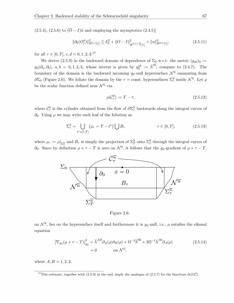
More precisely, we adopt the following plan: Let Σ30 be a spacelike hypersurface in Schwarzschild,

1The difference can be defined, for example, component wise for the two pairs of 2-tensors with respect to acommon coordinate system and measured in W s,p Sobolev spaces used in the literature [12].


v ur = 0 = uv = 1

(1,1)

Σ0

ΣT

Στ

Figure 2.3: The black hole region in Kruskal’s extension.

tangent2 at a single sphere of the singular hyperbola r = 0 inside the black hole; Figure 2.3.

We assume, without loss of generality,3 that the tangent sphere is (u = 1, v = 1) in Kruskal

coordinates (2.1.2). Consider now initial data sets (g,K) on Σ0 for the EVE (2.1.1), which have

the same singular behaviour to leading order at (u = 1, v = 1) with the induced Schwarzschild

initial data set (Sg, SK) on Σ0 and solve the EVE backwards, as depicted in the 2-dim Figure

2.3.

Realizing the above plan we thus prove the existence of a class of non-spherically symmetric

vacuum spacetimes for which (1) the leading asymptotics of the blow up of curvature and in

general of all the geometric quantities (metric, second fundamental form etc.) coincide with

their Schwarzschild counterparts, as one approaches the singularity, and (2) the singularity is

realized as the limit of uniformly spacelike hypersurfaces, which in the forward direction “pinch

off” in finite time at one sphere. Conversely, we visualise the backward evolution of (Σ0, g,K)

in the following manner: At ‘time’ τ = 0 the initial slice Σ0 is a two ended spacelike (3-dim)

hypersurface with a sphere singularity at (u = 1, v = 1). Once Σ0 evolves through (2.1.1),

it becomes instantaneously a regular spacelike hypersurface Στ , τ > 0 and the singular pinch

opens up; Figure 2.4.

The main difficulty to overcome in the backward local existence problem is the singularity on

Σ0, which of course renders it beyond the scope of the classical local existence theorem for the

Einstein equations [11], even its latest state of the art improvement by Klainerman-Rodnianski-

Szeftel [32], which requires at the very least the curvature of the initial hypersurface to be in

L2. For the Schwarzschild initial data set (Sg, SK) on Σ0, and hence for perturbed initial data

sets (g,K) with the same leading order geometry at (u = 1, v = 1), it is not hard to check

2The tangency here should be understood with respect to the differential structure of the Kruskal maximalextension induced by the standard u, v, θ, φ coordinates (2.1.2).

3Recall that the vector field tangent to the r = const. hypersurfaces (Figure 2.1) is Killing and we may henceutilize it to shift Σ0 and (u = 1, v = 1) to whichever point on uv = 1 we wish; Figure 2.3.


(u = 1, v = 1)Σ0

Σττ > 0

∂τ

Figure 2.4:

(§2.3) that the initial curvature is at the singular level

R 6∈ Lp(Σ0), ∇K 6∈ Lp(Σ0) p ≥ 5

4. (2.1.6)

Thus, we must rely heavily on the background Schwarzschild geometry to control the putative

backward evolution. A very useful fact for analysis is the opening up (smoothing out) of the

singularity (Figure 2.4) in the backward direction.

To our knowledge, general local existence results for the EVE (2.1.1) with singular initial

curvature not in L2 have been achieved only fairly recently by Luk-Rodnianski [35, 36] and Luk

[34] for the characteristic initial value problem, where they consider delta curvature singularities

and weak null singularities respectively. However, their context is much different from ours and

the results do not seem applicable to singularities of Schwarzschild type.

We proceed now to formulate a first version of our main results; for more precise statements,

in terms of weighted Sobolev spaces, see Theorems 2.4.6, 2.4.8, 2.6.6.

Theorem 2.1.1. There exists α > 0 sufficiently large, such that for every triplet (Σ0, g,K)

verifying:

(i) the constraints (2.1.5),

(ii) g = Sg + rαO, K = SK + rα−32u, where O, u are 2-tensors on Σ0 bounded in H4, H3

respectively,

(iii) ‖g − Sg‖L∞(Σ0) 1,

there exists a H4 local solution g to the Einstein vacuum equations (2.1.1) with initial data

(g,K), unique up to isometry, in the backward region to Σ0, foliated by Σττ∈[0,T ] (Figure

2.3); the time of existence T > 0 depends continuously on the norms of O, u and the exponent

α > 0.

The fact that non-trivial initial data sets in compliance with Theorem 2.1.1 exist is not at

all obvious nor standard. We need to show essentially that for any large parameter α > 0,

there exist non-spherically symmetric solutions to the constraint equations (2.1.5), having the

asymptotics (ii). We construct such solutions using the conformal method, which we set up in


§2.6.

Theorem 2.1.2. Let α > 0 be sufficiently large, consistent with Theorem 2.1.1. Then for every

choice of the transverse, traceless part of the second fundamental form and the mean curvature

on Σ0, compatible with the assumptions in Theorem 2.1.1, and verifying a reflection symmetry

condition, there exists a solution to the constraints (2.1.5) localized near the singular sphere

and verifying the asymptotics (ii) above.

Let us emphasize the fact that the above spacetimes are very special in that they agree

with Schwarzschild at the singularity to a high (but finite) order – this is captured by the large

exponent α > 0 in Theorem 2.1.1 – and therefore are non-generic. The need to choose α large

may be seen however natural to some extend in view of the instability of the Schwarzschild

singularity; from the point of view of the forwards-in-time problem. Indeed, the stable pertur-

bations of the Schwarzschild singularity must form a strict subclass of all perturbed vacuum

developments.

We note here that the restrictions imposed on the ‘free’ data for the constraints in Theorem

2.1.2 go beyond the largeness of the parameter α. The sole purpose of this is to overcome

some difficulties we encounter particularly for the constraint equations. We discuss this matter

further in Section §2.6.6.

2.1.1 Method of proof and outline

The largest part of the paper is concerned with the evolutionary part of the problem, i.e.,

proving Theorem 2.1.1. Due to the singular nature of backward existence problem described

above, Figure 2.3, the choice of framework must be carefully considered. The standard wave

coordinates approach [11] does not seem to be feasible in our situation; one expects that co-

ordinates would be highly degenerate at the singularity. Also, the widely used CMC gauge

condition is not applicable, since the mean curvature of the initial hypersurface Σ0 blows up

(§2.3). Instead, we find it more suitable to use orthonormal frames and rewrite the EVE one

order higher as a quasilinear Yang-Mills hyperbolic system of equations [40, 32], under a Lorenz

gauge condition,4 for the corresponding connection 1-forms. We recall briefly this framework

in §2.2.

However, even after expressing the EVE in the above framework, the singular level of initial

configurations do not permit a direct energy estimate approach. In addition to (2.1.6), one can

see (§2.3) that neither is the second fundamental form in L2

K 6∈ L2(Σ0). (2.1.7)

Note that the latter is at the level of one derivative in the metric. Hence, near the singularity

the perturbed spacetimes we wish to construct do not even make sense as weak solutions of

4The analogue of a wave gauge for orthonormal frames.


the EVE (2.1.1). Therefore, it is crucial that we use the background Schwarzschild spacetime

to recast the evolution equations in a new form having more regular initial data. We do this

in §2.4 by considering a new system of equations for the ‘difference’ between the putative

perturbed spacetime and Schwarzschild. The resulting equations have now regular initial data

and they are eligible for an energy method, but there is a price to pay. The coefficients of the

new system will depend on the Schwarzschild geometry and will necessarily be highly singular

at r = 0. We compute in §2.3 the precise blow up orders of the Schwarzschild connection

coefficients, curvature etc. Nevertheless, the issue of evolving singular initial data has become

the more tractable problem of finding appropriate weighted solution spaces for the final singular

equations.

In §2.4.2 we introduce the weighted Sobolev spaces which yield the desired flexibility in

proving energy estimates. The right weights are given naturally by the singularities in the

coefficients of the resulting equations, namely, powers of the Schwarzschild radius function r

with a certain analogy corresponding to the order of each term. After stating the general local

existence theorems in §2.4.3 and a more precise version of Theorem 2.1.1, we proceed to its proof

via a contraction mapping argument which occupies Section 2.5. Therein we derive the main

weighted energy estimates by exploiting the asymptotic analysis at r = 0 of the Schwarzschild

components (§2.3). It is necessary in our result that the power of r, α > 0, in the weighted

norms is sufficiently large; cf. assumption (ii) in Theorem 2.1.1. In the estimating process

certain critical terms are inevitably generated, because of the singularities in the coefficients

of the system we are working with; these terms are critical in that they appear with larger

weights than the ones in the energy we are trying to control and thus prevent the estimates

from closing. The exponent α > 0 is then picked sufficiently large such that these critical terms

have an overall favourable sign; this allows us to drop the critical terms and close the estimates.

The largeness of α forces the perturbed spacetime to agree asymptotically with Schwarzschild

to a high order at the singularity. Although the latter may seem restrictive, it is quite surprising

to us that there even exists a suitable choice of α which makes the argument work in the first

place. A closer inspection of our method reveals that it is very sensitive with respect to certain

asymptotics of the coefficients in the equations that happen to be just borderline to allow an

energy-based argument to close. The most important of these are the blow up order of the

sectional curvature (2.1.4) and the rate of growth of the Schwarzschild radius function r back-

wards in time. The latter corresponds to the ‘opening up’ rate of the neck pinch of the singular

initial hypersurface Σ0, Figure 2.4. In this sense the Schwarzschild singularity is exactly at the

threshold that our energy-based method can tolerate.

In the last section, §2.6, we study the constraint equations (2.1.5) in a perturbative manner

about the Schwarzschild singular initial data set (Sg, SK) on Σ0. We prove Theorem 2.1.2

by employing the inverse function theorem. Following the conformal approach, we prescribe

conformal data on Σ0 which asymptote to the corresponding Schwarzschild singular data at a

high order. Then we prove that the linearized conformal constraint map (about Schwarzschild)


is Fredholm in suitable weighted Sobolev spaces,5 capturing the asymptotics needed for Theorem

2.1.1 to be applied, see Proposition 2.6.5 which we prove in §2.6.2. In the case where Σ0 is

localized in a neighborhood of its singularity, the weighted elliptic estimates we derive can be

improved to yield that the conformal constraint map is actually an isomorphism. It is worth

noting that the solutions to the constraints that we produce have singular mean curvature.

2.1.2 Final Comments; Possible applications

The understanding of the question of stability of singularities in Einstein’s equations and the

behaviour of solutions near them is of great significance in the field. However, in general very

little is known. In terms of rigorous results, substantial progress has been made in spherical

symmetry in the presence of matter [14] [13] [46] [17]. Moreover, certain matter models enjoy the

presence of a monotonic quantity, which has been employed to study the stability of singularity

formation in the general non-symmetric regime, cf. recent work of Rodnianski-Speck [48] on the

FLRW big bang singularity. This is in contrast with the vacuum case of black hole interior and

the unstable nature of the Schwarzschild singularity. We hope that the method developed herein

can be employed to produce classes of examples of other singular solutions to the Einstein field

equations, which until now are only known to exist under very restrictive symmetry assumptions

and for which the general stability question may be out of reach.

The idea of constructing singular spacetimes by prescribing a specific singular behaviour

and solving for a spacetime ‘starting from the singularity’ is not new. There exists an extensive

literature regarding the construction of cosmological spacetimes exhibiting Kasner type singu-

larities at each point of their ‘big bang’ hypersurface6 using Fuchsian techniques [31, 45, 30].

However, the results in this category rely on the undesirable assumption of analyticity [1] and

or on various symmetry assumptions, see relevant work on Gowdy spacetimes [44, 47]. Yet, we

believe that the usual Fuchsian algorithm cannot be applied to Schwarzschild type singularities

due to their more singular nature.7

After our treatment of singular initial data containing a single sphere of uv = 1, a rea-

sonable next step would be to study whether the construction of non-spherically symmetric

vacuum spacetimes containing an arc of the singular hyperbola (Figure 2.3) is possible or even

the whole singularity r = 0. Certainly this is a more restrictive question and at first glance

not so obvious how to formulate it as a backward initial value problem problem for the EVE.

However, we hope that the method developed herein could help approach this direction.

Lastly, one could try to perform a global instead of a local construction by considering a

5We note that the spaces we use for the constraint equations differ from those we use for the evolutionarypart of the problem.

6At each point of the usual singular spacelike hypersurface the spacetime metric approaches asymptoticallythe metric of a Kasner spacetime, with the Kasner parameters generally varying from point to point, what iscalled AVTD behaviour [30].

7The reason should be understood in an effort to reduce the Einstein equations to Fuchsian type equationsfor a Schwarzschild type singularity. In this case the singularities in the coefficients of the reduced evolutionequations would be stronger than the ones encountered in the literature.


Cauchy hypersurface Σ0 extending to spacelike infinity. We expect this follows readily from

the work here, but we do not pursue it further. Perhaps a gluing construction could also be

achieved.

2.2 The Einstein equations as a quasilinear Yang-Mills system

The Einstein vacuum equations (2.1.1), by virtue of the second Bianchi identity, imply the van-

ishing of the divergence of the Riemann curvature tensor. Decomposing the latter with respect

to an orthonormal frame, which satisfies a suitable gauge condition, it results to a quasilinear

second order hyperbolic system of equations for the connection 1-forms corresponding to that

frame, which bears resemblance to the semilinear Yang-Mills [40]. Recently this formulation

of the EVE played a key role in the resolution of the bounded L2 curvature conjecture [32].

In this section we express the EVE (2.1.1) in the above setting, which we are going to use to

directly solve the Cauchy problem. This necessitates some technical details which are carried

out in Appendix B. Also, to avoid additional computations we write all equations directly in

scalar non-tensorial form.8

All indices below range from 0 to 3 unless otherwise stated.

2.2.1 Cartan formalism

Let (M1+3, g) be a Lorenzian manifold and let e0, e1, e2, e3 be an orthonormal frame; gab :=

mab = diag(−1, 1, 1, 1). Assume also that M1+3 has the differential structure of Σ × [0, T ],

where each leaf Σ × τ =: Στ is a 3-dim spacelike hypersurface. We denote the connection

1-forms associated to the preceding frame by

(AX)ij := g(∇Xei, ej) = −(AX)ji, (2.2.1)

where∇ is the g-compatible connection ofM1+3. Recall the definition of the Riemann curvature

tensor

Rµνij := g(∇eµ∇eνei −∇eν∇eµei, ej). (2.2.2)

By the former definition of connection 1-forms, using mab to raise and lower indices, we write

∇eaeb = (Aa)bkek.

Hence, we have

∇eµ∇eνei = ∇eµ(∇eνei)−∇∇eµeνei = ∇eµ((Aν)i

kek)− (Aµ)ν

k(Ak)icec

= eµ(Aν)ikek + (Aν)i

k(Aµ)kded − (Aµ)ν

k(Ak)icec

8It will be clear though which are the covariant expressions; see also [32].


Therefore, we get the following expression for the components of the Riemann curvature

Rµνij = eµ(Aν)ij − eν(Aµ)ij + (Aν)ik(Aµ)kj − (Aµ)i

k(Aν)kj (2.2.3)

− (Aµ)νk(Ak)ij + (Aν)µ

k(Ak)ij

or setting

([Aµ, Aν ])ij = (Aµ)ik(Aν)kj − (Aν)i

k(Aµ)kj (2.2.4)

we rewrite

(Fµν)ij := Rµνij = eµ(Aν)ij − eν(Aµ)ij − ([Aµ, Aν ])ij − (A[µ)ν]k(Ak)ij , (2.2.5)

where by standard convention

(A[µ)ν]k(Ak)ij := (Aµ)ν

k(Ak)ij − (Aν)µk(Ak)ij .

In the same manner we compute the covariant derivative of the Riemann tensor:

∇σRµνij = eσ(Fµν)ij − (Aσ)µk(Fkν)ij − (Aσ)ν

k(Fµk)ij

− (Aσ)ik(Fµν)kj − (Aσ)j

k(Fµν)ik

= eσ(Fµν)ij − (Aσ)k [µ(Fν]k)ij − ([Aσ, Fµν ])ij (2.2.6)

Recall the transformation law of the above quantities under change of frames: Let ei30 be

an orthonormal frame on M1+3 such that

ea = Okaek (2.2.7)

and let (AX)ij := g(∇X ei, ej) be the corresponding connection 1-forms. Then

(AX)ij = ObiOcj(AX)bc +X(Obi )O

cjmbc. (2.2.8)

In addition, from (2.2.7) we have

∇X ea = X(Oka)ek +Oka∇Xek(AX)a

ded = X(Oka)ek +Oka(AX)k

ded

or

X(Ola) = (AX)adOld −Oka(AX)k

l. (2.2.9)


2.2.2 ∇×Ric = 0

Now we proceed by assuming that the curl of the Ricci tensor of the metric g vanishes:

∇iRνj −∇jRνi = 0, (2.2.10)

where Rab := Rµabµ. A direct implication of the (contracted) second Bianchi identity is that

the divergence of the Riemann curvature tensor satisfies

∇µRijνµ = ∇iRνj −∇jRνi = 0. (2.2.11)

Thus, it follows from (2.2.6) that

eµ(Fµν)ij − (Aµ)k [µ(Fν]k)ij − ([Aµ, Fµν ])ij = 0 (2.2.12)

or by (2.2.5)

(Aν)ij − eµeν(Aµ)ij − eµ([Aµ, Aν ])ij − eµ((A[µ)ν]

k(Ak)ij)

(2.2.13)

= (Aµ)k [µ(Fν]k)ij + ([Aµ, Fµν ])ij ,

where := −e20 + e2

1 + e22 + e2

3 is the non-covariant box with respect to the frame ei. Since

[eµ, eν ] = ∇eµeν −∇eνeµ = (A[µ)ν]kek,

(2.2.13) takes the equivalent form

(Aν)ij − eνeµ(Aµ)ij = (A[µ)ν]kek(Aµ)ij + eµ([Aµ, Aν ])ij + eµ

((A[µ)ν]

k(Ak)ij)

+ (Aµ)k [µ(Fν]k)ij + ([Aµ, Fµν ])ij , (2.2.14)

ν, i, j = 0, 1, 2, 3. We remark that (2.2.14) is an equation of scalar functions.

2.2.3 Choice of gauge

Note that the preceding equation is not of hyperbolic type. We convert (2.2.14) into a quasilinear

hyperbolic system of equations by imposing a Lorenz gauge condition on the orthonormal frame

ei30:9

A2 = (divA)ij := ∇µ(Aµ)ij − (A∇eµeµ)ij = eµ(Aµ)ij − (Aµ)µk(Ak)ij , (2.2.15)

where by A2 we denote some quadratic expression in the connection coefficients (Aν)ij varying

in ij. This a freedom one has in choosing the frame ei; see Lemma B.0.12. Under (2.2.15), the

9A wave type gauge essentially for ei. The Coulomb gauge is another alternative which is used in [32]. Wedo not employ it here.


equation (2.2.14) becomes the quasilinear second order

(Aν)ij = (A[µ)ν]kek(Aµ)ij + eµ([Aµ, Aν ])ij + eµ

((A[µ)ν]

k(Ak)ij)

+ (Aµ)k [µ(Fν]k)ij + ([Aµ, Fµν ])ij + eν(A2) + eν((Aµ)µ

k(Ak)ij)

(2.2.16)

2.2.4 The reduced equations; Initial data for EVE

Following (2.2.11)-(2.2.16) we actually see that the equation

∇iRνj −∇jRνi+eν(divA−A2

)ij

(2.2.17)

=: Hνij = (LHS of (2.2.16))− (RHS of (2.2.16)),

holds true for every Lorentzian metric g and orthonormal frame ei30, without any additional

assumptions or gauge condition. We call Hνij = 0, i.e., the system (2.2.16), the reduced

equations. We note that even after the gauge fixing, the reduced equations are not equivalent

to the EVE (2.1.1), but only imply the vanishing of the curl of the Ricci tensor (2.2.10).

However, one may suitably prescribe initial data for (2.2.16) such that they lead to solutions

of the EVE and which are consistent with the Lorenz gauge condition (2.2.15).

Now we address the initial value problem for the reduced equations Hνij = 0 aiming to

the EVE. To solve the equation (2.2.16) one needs an equation relating the evolution of the

orthormal frame ei30 to that of the connection 1-forms. Let ∂0, ∂1, ∂2, ∂3 be a reference frame10

in Σ× [0, T ] (∂0 transversal direction). We express ei in terms of ∂a:

ei = Oai ∂a (2.2.18)

By virtue of the diffeomorphism invariance of the EVE, we may assume that the timelike unit

vector of the orthonormal frame ei30 of the spacetime we solve for is e0 = ∂0. Doing so we

deduce

∂0(Oai ) = Le0(∂a(ei)

)= L∂0(∂a)ei + ∂a([∂0, ei]) = ObiL∂0(∂a)∂b + ∂a([e0, ei]),

where L denotes the Lie derivative and ∂a is the 1-form dual to ∂a. Setting [∂0, ∂b] =: Γc[0b]∂c

we rewrite

∂0(Oai ) = −ObiΓa[0b] + (A[0)i]kOak. (2.2.19)

Now we proceed to formulate the necessary and sufficient conditions on the initial data set of

the reduced equations (2.2.16), coupled to (2.2.19), such that the corresponding solution yields

a solution to the EVE. The following proposition is proved in §B.0.5.

10Not orthonormal or coordinates, simply a basis frame.


Proposition 2.2.1. Let (Aν)ij , Oai be a solution of (2.2.16),(2.2.19), arising from initial con-

figurations subject to

(Aν)ij(τ = 0) = −(Aν)ji(τ = 0) ∂0(Aν)ij(τ = 0) = −∂0(Aν)ji(τ = 0) (2.2.20)

Oa0(τ = 0) = I0a

and

(divA)ij −A2 = 0 ⇐⇒ eµ(Aµ)ij − (Aµ)µk(Ak)ij −A2 = 0 (2.2.21)

Ricab(g) = 0 ⇐⇒ eµ(Aν)iµ − eν(Aµ)iµ − ([Aµ, Aν ])iµ − (A[µ)ν]k(Ak)iµ = 0

on Σ0. Then the latter solution corresponds to an Einstein vacuum spacetime (M1+3, g) and

furthermore the frame ei30 (2.2.18) is g-orthonormal, e0 = ∂0, and satisfies the Lorenz gauge

condition (2.2.15).

Remark 2.2.2. Note that the second part of (2.2.21) includes the constraints (2.1.5); R0b =

R00 − 12R = 0, b = 1, 2, 3, on Σ0. The condition (2.2.21) is necessary and sufficient (as we

show in B.0.5) to yield the propagation of the gauge and the EVE themselves. Once we have

chosen the orthonormal frame initially and the initial data components (A0)ij(τ = 0), which

correspond to the ∂0 derivative of ei30, then the rest of the initial data set of (2.2.16) is fixed

by the condition (2.2.21), i.e., the Lorenz gauge and the EVE on the initial hypersurface Σ0,

see Remark B.0.13.

2.3 The Schwarzschild components

We fix an explicit Schwarzschild orthonormal reference frame and compute the corresponding

connection coefficients, which we then use to find the leading asymptotics of the second funda-

mental form and curvature of the initial singular hypersurface Σ0 in Schwarzschild. Knowing

the precise leading blow up behaviour of these quantities is crucial for the study of the back-

wards well-posedness in the next section. For distinction, we denote Schwarzschild components

with an upper left script S .

Let us consider a specific foliation of spacelike hypersurfaces Στ , τ ∈ [0, T ], for the backward

problem in a neighbourhood of (u = 1, v = 1); Figure 2.3. For convenience11 let

Στ : −1

2(u+ v) + 1 = τ (u, v) ∈ (1− ε, 1 + ε)2, τ ∈ [0, T ]. (2.3.1)

11It is easy to see that the following leading asymptotics we derive are independent of the particular choice offoliation.


Σ0

Στ

ΣT

u v

∂τ

r = 0 = uv = 1

∂x

(1,1)

Figure 2.5: The foliation (2.3.1) in the interior of the black hole.

In temporal and spatial coordinates τ, x

∂τ := −∂u − ∂v, ∂x := ∂u − ∂v (2.3.2)

x =1

2(u− v),

the metric (2.1.2) takes the form

Sg = −Ω2dτ2 + Ω2dx2 + r2(dθ2 + sin2 θdφ2), Ω2 =32M3

re−

r2M . (2.3.3)

By (2.1.3),(2.3.2) r is related to τ, x via

(1− τ)2 − x2 = (1− r

2M)e

r2M , (2.3.4)

from which one can derive the following formulas:

∂τr =Ω2

4M(1− τ), ∂xr =

Ω2

4Mx (2.3.5)

∂τΩ2 = − Ω4

4M(1

r+

1

2M)(1− τ), ∂xΩ2 = − Ω4

4M(1

r+

1

2M)x

Remark 2.3.1. The above first two identities yield the leading asymptotics:

r2 ∼ 16M2(x2

2+ τ), as τ, x→ 0. (2.3.6)

Directly from the form of the induced metric on Στ ,

Sg = Ω2dx2 + r2(dθ2 + sin2 θdφ2), (2.3.7)


we compute the corresponding induced volume form

dµSg = Ωr2 sin θdxdθdφ =[4√

2M32 r

32 +O(r2)

]sin θdxdθdφ (2.3.8)

and its rate of change along ∂τ using (2.3.5):

∂τdµSg =[12M2

r2(1− τ) +O(

1

r)]dµSg. (2.3.9)

Normalizing, we define the Schwarzschild orthonormal frame

∂0 =1

Ω

∂

∂τ∂1 =

1

Ω

∂

∂x∂2 =

1

r

∂

∂θ∂3 =

1

r sin θ

∂

∂φ(2.3.10)

and the relative connection coefficients S(Aµ)ij = Sg(S∇∂µ∂i, ∂j) associated to it. A tedious

computation12 shows that the non-zero components read

S(A0)01 = − Ω

8M(1

r+

1

2M)x

S(A1)01 = − Ω

8M(1

r+

1

2M)(1− τ)

S(A2)02 = S(A3)03 =Ω

4M

1− τr

(2.3.11)

S(A2)12 = S(A3)13 =Ω

4M

x

r

S(A3)23 =cot θ

r

Recall the (spacetime) divergence formula of the connection 1-forms X → S(AX)ij

S(divA)ij := ∂µS(Aµ)ij − S(A∇∂µ∂µ)ij = ∂µS(Aµ)ij − S(Aµ)µbS(Ab)ij (2.3.12)

Utilizing (2.3.5) and (2.3.11), we check that the first order term in the RHS of (2.3.12) vanishes

∂µS(Aµ)ij = 0, (2.3.13)

leaving

S(divA)ij = S(A3)23S(A2)ij . (2.3.14)

Remark 2.3.2. Thus, the orthonormal frame (2.3.10) satisfies a Lorenz gauge type condition

(2.2.15).

12One may calculate the connection coefficients using the Koszul formula

S(Aµ)ij =1

2

[Sg([∂µ, ∂i], ∂j)− Sg([∂i, ∂j ], ∂µ) + Sg([∂j , ∂µ], ∂i)

]


Remark 2.3.3. Summarizing the above identities and formulas we obtain the following leading

asymptotics at r = 0:

∂0 ∼1

4√

2M32

r12∂τ ∂1 ∼

1

4√

2M32

r12∂x

|SA| ≤ C

r32

|∂(k)SA| ≤ C

r(k+1) 32

, (2.3.15)

where C depends on M > 0 and k. Notice that the latter asymptotics are sharp for k = 0

and when ∂(k) = ∂(k)0 . In fact, the components of the second fundamental form of the slices

SKii = S(Ai)0i, i = 1, 2, 3, are exactly at this level. In more geometric terms we have (up to

constants)

|SK| ∼ 1

r32

|trSgSK| ∼1

r32

|SR| ∼ 1

r2. (2.3.16)

Thus, employing (2.3.8),(2.3.6) for τ = 0, we see that both the scalar curvature and the second

fundamental of the initial singular hypersurface Σ0 are far from being square integrable∫Σ0

|SK|2dµSg ∼∫ ε

0

1

x3x

32dx =

∫ ε

0

1

x32

dx = +∞∫Σ0

|SR|2dµSg ∼∫ ε

0

1

x4x

32dx =

∫ ε

0

1

x52

dx = +∞ (2.3.17)

The same holds for the mean curvature of Σ0. In fact, a similar calculation shows trSgSK 6∈ Lp,

p ≥ 53 .

Remark 2.3.4. The precise leading asymptotics of all computed quantities in this section play

a crucial role in the analysis of the backward existence problem and the proofs of the main

theorems in the next section. However, exact formulas, like (2.3.11), are not really needed. We

could have chosen as well a foliation of the form Στ : τ = f(x), instead of (2.3.1), i.e., τ = const.,

for some smooth function f(x), f ′(0) = 0. It is easy to see by computing the induced metric

and second fundamental form that the leading asymptotics of all relevant quantities of interest

remain the same.

2.4 The local-in time backwards well-posedness

2.4.1 Perturbed spacetime; A transformed system

Let (g,K) be a perturbation of the Schwarzschild initial data set (Sg, SK) on Σ0, verifying the

constraints (2.1.5), and let ei31 be an orthonormal frame of (Σ0, g). We fix a reference frame

∂i30 in M1+3 = Σττ∈[0,T ], namely, the Schwarzschild orthonormal frame (2.3.10); Figure


2.5. Let ei30, e0 = ∂0, be a frame extension in M1+3 expressed in terms of ∂d via

ec = Odc∂d. (2.4.1)

Consider now the (unique) metric g for which ei is orthonormal, gab := mab = diag(−1, 1, 1, 1),

and the corresponding connection coefficients (Aν)ij = g(∇eνei, ej). Then Proposition 2.2.1

asserts that the EVE (2.1.1) for g, under the Lorenz gauge condition13

(divA)ij = (A3)23(A2)ij , (2.4.2)

reduce to the system of scalar equations

(Aν)ij = (A[µ)ν]kek(Aµ)ij + eµ([Aµ, Aν ])ij + eµ

((A[µ)ν]

k(Ak)ij)

+ (Aµ)k [µ(Fν]k)ij + ([Aµ, Fµν ])ij + eν((A3)23(A2)ij

)+ eν

((Aµ)µ

k(Ak)ij)

(2.4.3)

∂0(Odc ) =−ObcS(A[0)b]d + (A[0)c]

kOdk, ν, i, j, c, d ∈ 0, 1, 2, 3

where := −e20 + e2

1 + e22 + e2

3 and S(A[0)b]d = [∂0, ∂b]

d.

However, the system (2.4.3) has singular initial data in the Schwarzschild background which

do not permit an energy approach directly. For this reason we recast the equations in a way

that captures the closeness to the Schwarzschild spacetime. Let

(uν)ij := (Aν)ij − S(Aν)ij : Σττ∈[0,T ] → R ν, i, j ∈ 0, 1, 2, 3, (2.4.4)

where the components S(Aν)ij are the Schwarzschild connection coefficients corresponding to

the frame ∂i30 (2.3.10) and they are given by (2.3.11). We are going to use these new functions

to control the evolution of the perturbed spacetime.

Consider now the analogous system to (2.4.3) satisfied by the Schwarzschild componentsS(Aν)ij , ∂c. In view of the asymptotics (2.3.15), we define Γq to be a smooth function satisfying

the bound

|Γq| ≤Cqrq

|∂(k)Γq| ≤Cq,k

rq+32k, (2.4.5)

for constants Cq, Cq,k depending on M > 0. Taking the difference of the two analogous systems

we obtain a new system for the functions (uν)ij , Odc − Icd written schematically in the form:

hab∂a∂b(uν)ij = OΓ 32∂u+OΓ3u+OΓ 9

2(O − I) +OΓ3∂(O − I)

+ Γ3u2 +Ou∂u+ u3 +O∂(O − I)∂u (2.4.6)

∂0(Odc − Icd) = Γ 32(O − I) + (O − I)u+ u,

13We choose now a specific type based on the one satisfied by the Schwarzschild reference frame (2.3.14).


where

hab := mcdOacObd = gab (2.4.7)

and each term in the RHS denotes some algebraic combination of finite number of terms of the

depicted type (varying in ν, i, j) where the particular indices do not matter.

Remark 2.4.1. Evidently, the systems (2.4.3) and (2.4.6) are equivalent. The benefit is that

the assumption on the perturbed spacetime, being close to Schwarzschild, implies that the

functions (uν)ij , Odc − Icd are now small and regular. Thus, we have reduced the evolutionary

problem to solving the PDE-ODE system of equations (2.4.6). However, the issue of singular

initial data in (2.4.3) has become an issue of singularities in the coefficients of the resulting

equations (2.4.6), at τ = x = 0, which do not make it possible to apply the energy procedure

in standard spaces; see also (2.3.17). These singularities, in large part, are due to the intrinsic

curvature blow up and cannot be gauged away; in particular the coefficients Γ3 of the potential

terms in (2.4.6) correspond to the Schwarzschild curvature (2.1.4). Some of the functions Γq

that appear in (2.4.6), expressed in terms of Schwarzschild connection coefficients (2.3.11) and

their derivatives, are less singular than (2.4.5), but representatives of the exact bound do appear

in all the terms.

Remark 2.4.2. Another crucial asymptotic behaviour that our method heavily depends on is

that of the radius function r. According to (2.3.6), we observe that the best L∞Στ bound one

could hope for the ratio 1/r2 is of the form

‖ 1

r2‖L∞(Στ ) ≤

C

τ, (2.4.8)

which obviously fails to be integrable in time τ ∈ [0, T ], for any T > 0. This fact lies at the

heart of the difficulty of closing a Gronwall type estimate.

2.4.2 The weighted Hs spaces

In order to study the well-posedness of (2.4.6) we introduce certain weighted norms. It turns

out that the weights which yield the desired flexibility in obtaining energy estimates are the

following.

Definition 2.4.3. Given α > 0 and τ ∈ [0, T ], we define the (time dependent) weighted Sobolev

space Hs,α[τ ], as a subspace of the standard Hs space on Στ with the Schwarzschild induced

volume form satisfying:

Hs,α[τ ] : u ∈ Hs(Στ ), ‖u‖2Hs,α[τ ] :=∑k≤s

∫Στ

[∂(k)u]2

r2α−3(k−1)dµSg < +∞, (2.4.9)


where by ∂(k) we denote any order k combination of directional derivatives with respect to the

components ∂1, ∂2, ∂3 of the Schwarzschild frame (2.3.10). For convenience, we drop τ from the

notation whenever the context is clear.

Remark 2.4.4. Observe that the weights in the norm ‖ · ‖Hs,α in (2.4.9) blow up only at

τ = 0, x = 0. For τ > 0 fixed, the weights are uniformly bounded above by some positive

constant Cτ , which becomes infinite as τ → 0+. The dependence of the power 2α− 3(k− 1) on

the number k of derivatives corresponds to the singularities in the coefficients of the equation

(2.4.6).

Lemma 2.4.5. The weighted Hs,α spaces satisfy the properties:

Hs1,α ⊂ Hs2,α s1 < s2

r−32lu ∈ Hs,α− 3

2l, whenever u ∈ Hs,α (2.4.10)

∂(k)u ∈ Hs−k,α− 32k k ≤ s, u ∈ Hs,α

Proof. They are immediate consequences of Definition 2.4.3 and and the fact that

|∂1(r−32l)| ≤ Clr− 3

2l− 1

2 |∂2(r−32l)| = |∂3(r−

32l)| = 0,

cf. (2.3.5), (2.3.10).

2.4.3 Local existence theorems

Let

E(u,O;α, T ) :=

3∑ν,i,j=0

[sup

τ∈[0,T ]

(‖(uν)ij‖2H3,α + ‖∂0(uν)ij‖2

H2,α− 32

)+

∫ T

0

(‖(uν)ij‖2H3,α+1 + ‖∂0(uν)ij‖2

H2,α− 12

)dτ

](2.4.11)

+3∑

c,d=0

[sup

τ∈[0,T ]‖Odc − Icd‖2

H3,α+32

+

∫ T

0‖Odc − Icd‖2

H3,α+52dτ

]

be the total weighted energy of the functions (uν)ij , Odc−Icd defined in Σττ∈[0,T ] (2.3.1), Figure

2.3.1, the backward domain of dependence of Σ0 with respect to the metric g we are solving

for. Since the actual domain depends on the unknown solution, it will be fully determined in

the end; see Section 2.5. For brevity we denote by

E0 :=∑

ν,i,j∈0,1,2,3

[‖(uν)ij(τ = 0)‖2H3,α + ‖∂0(uν)ij(τ = 0)‖2

H2,α− 32

](2.4.12)

+∑

c,d∈0,1,2,3

‖Odc − Icd‖2H3,α+3

2 (Σ0)


the energy at the initial singular slice Σ0.

The following theorem is our first main local well-posedness result for the system (2.4.6),

whose proof occupies Section §2.5.

Theorem 2.4.6. There exist α > 0 sufficiently large and ε > 0 small such that if

E0 < +∞ ‖Odc − Icd‖L∞(Σ0) < ε, c, d = 0, 1, 2, 3, (2.4.13)

then the system (2.4.6) admits a unique solution, up to some small time T = T (E0, α) > 0, in

the spaces

(uν)ij ∈ C([0, T ];H3,α) ∩ L2([0, T ];H3,α+1) ν, i, j ∈ 0, 1, 2, 3∂0(uν)ij ∈ C([0, T ];H2,α− 3

2 ) ∩ L2([0, T ];H2,α− 12 ) (2.4.14)

Odc − Icd ∈ C([0, T ];H3,α+ 32 ) ∩ L2([0, T ];H3,α+ 5

2 ) c, d ∈ 0, 1, 2, 3

Remark 2.4.7. (i) The second part of condition (2.4.13), ε > 0 small, is necessary for the

equation (2.4.6) to be hyperbolic, yielding sufficient pointwise control on the hab’s (2.4.7)

|hbb −mbb| < 1

2|hbc| ≤ Cε2, b, c = 0, 1, 2, 3, b 6= c. (2.4.15)

It could be obviously replaced by the stronger assumption that E0 < ε, since the energy

E(u,O;α, T ) controls the L∞ norm of u,O by standard Sobolev embedding.

(ii) How large the exponent α has to be depends on the coefficients of the system (2.4.6). In

the final inequalities in §2.5 α > 0 is picked large enough so that certain ‘critical’ terms can be

absorbed in the LHS and the estimates can close.

The above theorem is a local existence result for the system (2.4.6). Imposing now the

proper conditions on the initial data set of (2.4.6), the solution (2.4.14) yields a solution of

(2.4.3) which in turn corresponds to an Einstein vacuum spacetime (2.1.1).

Theorem 2.4.8. Let α, ε be such as in Theorem §2.4.6 and let (Σ0, g,K) be an initial data

set for the Einstein vacuum equations (2.1.1) satisfying the constraints (2.1.5), such that the

components

(uν)ij ∈ H3,α(Σ0) ν, i, j = 1, 2, 3, (2.4.16)

Odc − Icd ∈ H3,α+ 32 (Σ0) ‖Odc − Icd‖L∞(Σ0) < ε c, d = 1, 2, 3, (2.4.17)

computed with respect to an orthonormal frame ei31 on (Σ0, g), and

(ui)0j(τ = 0) := Kij − SKij ∈ H3,α(Σ0) i, j = 1, 2, 3. (2.4.18)


Then, there exists a solution g to the EVE (2.1.1) in the backward region to Σ0, foliated by

Στt∈[0,T ], with induced initial data set (g,K) on Σ0 and an orthonormal frame extension

ei30 for which the corresponding (spacetime) functions (uν)ij , Odc − Idc (2.4.4),(2.4.1) lie in the

spaces (2.4.14).

If in addition Odc − Icd ∈ C([0, T ];H4,α+ 32 ), c, d = 1, 2, 3, then the Einsteinian vacuum develop-

ment is unique up to isometry.

The fact that such (non-spherically symmetric) initial data sets (Σ0, g,K) exist, in compli-

ance with Theorem 2.4.8, is shown in §2.6.

Proof of Theorem 2.4.8. We want to invoke Theorem 2.4.6. For this purpose, we prescribe

initial data for the system (2.4.6):

(i) The components (2.4.16), (2.4.17), (2.4.18) are given.

(ii) Since in the beginning of §2.4.1 we assumed e0 = ∂0 and since ei31 is initially tangent to

Σ0, we set

Ob0(τ = 0) = I0b O0

a(τ = 0) = Ia0 a, b = 0, 1, 2, 3. (2.4.19)

(iii) We (freely) assign14

(u0)ab(τ = 0) := (A0)ab − S(A0)ab ∈ H3,α(Σ0), a, b = 0, 1, 2, 3. (2.4.20)

Once we have prescribed the above, the components ∂0(uν)ij(τ = 0) are fixed by the assumption

(2.2.21) on the initial data of the original system (2.4.3); see Remark B.0.13. Indeed, subtracting

the corresponding Schwarzschild components from (B.0.15),(B.0.16), which obvisouly satisfy the

same initial relations, cf. (2.3.14), we obtain schematically:

∂0(uν)ij = O∂au+ Γ 32u+ Γ3(O − I) + u2 on Σ0, a = 1, 2, 3. (2.4.21)

By (2.4.10) and standard Sobolev embedding we conclude that

∂0(uν)ij(τ = 0) ∈ H2,α− 32 ν, i, j = 0, 1, 2, 3. (2.4.22)

Thus, the assumption (2.4.13) is verified and Theorem 2.4.6 can be invoked. From Proposition

2.2.1 it follows that the solution (2.4.14) of (2.4.6) and hence of (2.4.3) yields indeed an Einstein

vacuum spacetime (Στ∈[0,T ], g).

To prove uniqueness (up to isometry) we rely on the uniqueness statement in Theorem

2.4.6. Suppose there is another Einsteinian vacuum development (M1+3, g) of the initial data

set (Σ0, g,K), diffeomorphic to Σττ∈[0,T ], satisfying the hypothesis (2.4.16), (2.4.17), (2.4.18);

defined by pulling back the relevant quantities through the preceding diffeomorphism, taking

14The functions (u0)ab(τ = 0) or equivalently (A0)ab(τ = 0) fix the ∂0 derivative of the frame ei30 on Σ0; seeLemma B.0.12 and Remark B.0.13.


differences etc. In order to use the uniqueness statement in Theorem 2.4.6, we need the two

spacetimes to have the same initial data for the system (2.4.6). The part of the initial data

set given by the assumptions in the statement of Theorem 2.4.8 is of course identical for both

spacetimes. The remaining components that we want to agree, other than the (u0)ab(τ = 0)’s, as

noted in the previous paragraph, can be fixed by condition (2.2.21). Therefore, we get identical

initial data components for the system (2.4.6) by constructing a Lorenz gauge frame (2.4.2)

ei30 for g, which is initially equal to ei30 on Σ0 and such that (u0)ab(τ = 0) = (u0)ab(τ = 0)

as well; see Lemma B.0.12. The only assumption to be verified is the well-posedness of the

system (B.0.1) for functions in the solution spaces (2.4.14), after taking differences with the

equation for the frame ei30. However, this falls in the category of the system (2.4.6) [in fact

simpler, being semilinear] to which Theorem 2.4.6 can be applied. The extra derivative that

we have to assume in order to close, Odc − Icd ∈ H4,α+ 32 , is due to the divA term in the RHS of

(B.0.1).

2.5 Proof of Theorem 2.4.6

Throughout this section we will use the notation X . Y to denote an inequality between the

quantities X,Y of the form X ≤ CY , where C is an absolute positive constant depending

only on the Schwarzschild mass M > 0. The same for the standard notation O(X), for a

quantity bounded by |O(X)| ≤ CX, X > 0. Furthermore, all the estimates regard only the

Schwarzschild region foliated by Σττ∈[0,T ]; Figure 2.3.

2.5.1 Proof outline

We prove Theorem 2.4.6 via a contraction mapping argument. First we establish an energy

estimate in the relevant weighted H3 spaces in §2.5.3. Then we obtain a contraction, in §2.5.4,

in the corresponding spaces of one derivative less, see (2.5.48), which together with the energy

estimate yield the desired solution (2.4.14).

To derive these estimates we have to eliminate some critical terms which are generated due to

the singularities in the coefficients of the equations, having larger weights than the ones in the

norm (2.4.9), and which prevent us from closing (see Propositions 2.5.3,2.5.6). This is where

the role of the weights (2.4.9) comes in. The parameter α > 0 helps generate critical terms

with a favourable sign. Being large enough, but finite, α provides an overall negative sign for

the critical terms, hence, rendering them removable from the RHS of the final inequalities.

This enables us to close the estimates and complete the proof. The precise asymptotics of the

singularities in the coefficients of the equations (2.4.6), at τ = x = 0, and the opening up rate

of the radius function r in τ > 0 play a crucial role here.15

15If we were to tweak the leading orders just by ε > 0, the previous procedure would fail no matter how largeα > 0 is to begin with.


2.5.2 Basic estimates

Let v be a scalar function defined on Στ , represented by

v ψτ : Uτ → R, (2.5.1)

where ψτ : Uτ → Στ is the (x, θ, φ) coordinate chart. We recall some standard inequalities: the

classical Sobolev embedding of H2(U) in L∞(U)

‖v‖L∞(U) . ‖v‖H2(U) (2.5.2)

and the interpolation inequality

‖v‖L4(U) ≤ C‖v‖14

L2(U)‖∇v‖

34

L2(U)v ∈ C∞c (U), (2.5.3)

for a bounded domain U ⊂ R3 with (piecewise) C2 boundary. In the following proposition v is

assumed to be regular enough such that the RHSs make sense.

Proposition 2.5.1. For a general function v : Στ → R, τ ∈ [0, T ], with the appropriate

regularity, the following inequalities hold:

The L∞ bound

‖ vrk‖L∞(Στ ) . (k + 1)2‖v‖

H2,k+3+14 (Στ )

(2.5.4)

and the L4 estimate

‖ vrk‖L4(Στ ) . (k + 1)

34 ‖v‖

H1,k+1+14 (Στ )

. (2.5.5)

Proof. From (2.5.2) we have

‖ vrk‖L∞(Στ )

(2.5.1)= ‖ v

rk ψτ‖L∞(Uτ ) . ‖

v

rk ψτ‖H2(Uτ )

. (k + 1)2‖v‖H2,k+3+1

4 (Στ ).

(substituting (2.3.8) and the frame (2.3.10))

We argue similarly in the case of (2.5.5).

2.5.3 Energy estimate in H3,α

We set up now the iteration scheme we are going to follow. Let u,O := (uν)ij , Odc :

ν, i, j, c, d = 0, 1, 2, 3 be a set of spacetime functions in the solution spaces (2.4.14), verify-


ing |Odc − Icd| < ε initially on Σ0. We assume without loss of generality16

E(u,O;α, T ) ≤ 2E0. (2.5.6)

We also assume

‖∂0(Odc)‖2H2,α[τ ] . E2

0 + E0 ∀τ ∈ [0, T ], c, d = 0, 1, 2, 3. (2.5.7)

Iteration step: Consider the following linear version of the system (2.4.6), where we replace

the functions u,O in the following specific terms by the corresponding ones from the set u,O:

hab∂a∂b(uν)ij = OΓ 3

2∂u+OΓ3u+OΓ 9

2(O − I) +OΓ3∂(O − I)

+ Γ3u2 +Ou∂u+ u3 +O∂(O − I)∂u (2.5.8)

∂0(Odc − Icd) = Γ 32(O − I) + (O − I)u+ u,

where hab

= mcdOacO

bd. Observe that we kept in the RHS of (2.5.8) the functions u,O attached

to the most singular coefficients of the system. This is actually very important to our strategy

in order to avoid further complications.

We assume now there exists a solution (uν)ij , Odc − Icd of (2.5.8) lying in the solution space

(2.4.14). The existence of such a solution is based mainly on the energy estimate we will derive

below and a standard duality argument which we omit.

Claim: For a chosen large enough α > 0 and T > 0 sufficiently small (depending on E0, α) the

following estimate holds

E(u,O;α, T ) ≤ 2E0. (2.5.9)

The preceding H3-weighted energy estimate, cf. (2.4.11), will be used in the next subsection to

close the contraction argument that yields the existence and uniqueness of the solution (2.4.14)

to (2.4.6). Now we begin the proof of (2.5.9):

First note that by the fundamental theorem of calculus, following a ∂0 integral curve and

employing (2.5.4), we readily obtain from our initial assumptions and (2.5.7) the pointwise

bound

supτ∈[0,T ]

‖O − I|‖L∞(Στ ) ≤ ε+ CTE0 < 2ε, (2.5.10)

provided α ≥ 12 + 3 + 1

4 and T < εCE0 .

All the more, directly from the ODE in (2.5.8) we deduce the estimate: [applying the bounds

16Any assumptions that we make on the functions u,O, we must derive for the next set of functions u, f below.


(2.5.4), (2.5.6) to (O − I)u and employing the asymptotics (2.4.5)]

‖∂0(Odc )‖2H2,α[τ ] . E20 + ‖O − I‖2

H2,α+32 [τ ]

+ ‖u‖2H2,α[τ ], (2.5.11)

for all τ ∈ [0, T ], c, d = 0, 1, 2, 3.17

We derive (2.5.9) in the backward domain of dependence of Σ0 w.r.t. the metric (gab)u :=

gu(∂a, ∂b), a, b = 0, 1, 2, 3, whose inverse is given by gabu := hab

; compare to (2.4.7). The

boundary of the domain is the backward incoming gu-null hypersurface N u emanating from

∂Σ0 (Figure 2.6). We foliate the domain by the τ = const. hypersurfaces Σuτ inside N u. Let ρ

be the scalar function defined near N u via

ρ(Cuτ ) := T − τ, (2.5.12)

where Cuτ is the cylinder obtained from the flow of ∂Σuτ backwards along the integral curves of

∂0. Using ρ we may write each leaf of the foliation as

Σuτ =

⋃t∗∈[τ,T ]

ρτ = T − t∗⋃Bτ τ ∈ [0, T ], (2.5.13)

where ρτ := ρ∣∣Σuτ

and Bτ is simply the projection of ΣuT onto Σu

τ through the integral curves of

∂0. Since by definition ρ + τ − T is zero on N u, it follows that the gu-gradient of ρ + τ − T ,

Σ0

Σuτ

ΣuT

N u N u

∂0

Cuτ

Bτ

x = 0

Figure 2.6:

on N u, lies on the hypersurface itself and furthermore it is gu-null, i.e., ρ satisfies the eikonal

equation

∣∣∇gu(ρ+ τ − T )∣∣2gu

= hAB∂A(ρ)∂B(ρ) + Ω−2h

00+ 2Ω−1h

A0∂A(ρ) (2.5.14)

= 0 on N u,

where A,B = 1, 2, 3.

17This estimate, together with (2.5.9) in the end, imply the analogue of (2.5.7) for the functions ∂0(Odc ).


Remark 2.5.2. The backward domain of definition of the variables u,O−I depends on u,O−I.

For the iteration scheme and the contraction mapping argument in §2.5.4 to be well-defined,

all functions involved in the process must have a common domain of definition. To solve this

issue is to begin with a slightly ‘larger’ initial hypersurface Σ0 ⊃ Σ0 extending Σ0 at both ends

and to solve at each iteration step for the new variables in a ‘smaller’ domain contained in the

interior of the domain of the previous iterate by shrinking the initial hypersurface Σ0. Since

we are also proving a contraction mapping at the same time (see §2.5.4) we can make sure that

the shrinking of Σ0 stops at Σ0 giving the final backward domain in the limit.

We define the following adapted energy, which controls the part of the total energy (2.4.11)

that refers to u:

Es+1,α[u](τ) :=1

2

∑ν,i,j

∑|J |≤s

∫Σuτ

[− h00

[∂0(uν)ij,J

]2r2α−3|J | (2.5.15)

+ hAB ∂A(uν)ij,J

rα−32|J |

∂B(uν)ij,J

rα−32|J |

+(uν)2

ij,J

r2α−3(|J |−1)

]dµSg,

where (uν)ij,J := ∂(J)(uν)ij and J is a spatial multi-index (containing only directions ∂1, ∂2, ∂3).

It is evident from (2.5.10), hab

= mcdOacO

bd, that E3,α is equivalent to the weighted H3,α ×

H2,α− 32 norm of u on Σu

τ .

We summarize in the following proposition the main energy estimates derived below.

Proposition 2.5.3. The following two energy estimates hold:

∂τE3,α[u] + 8M2e−1(1− τ)αE3,α+1[u]

. (E120 + E0 + α2 + α3E0)E3,α[u] + E3,α+1[u] + E0‖O − I‖2

H3,α+32

(2.5.16)

+ ‖O − I‖2H3,α+5

2+ α3E2

0 + E30

1

2∂τ∑c,d


2+ 4M2e−1(1− τ)α

∑c,d


2(2.5.17)

. ‖O − I‖2H3,α+5

2+ E3,α+1[u] + E2

0 ,

for all τ ∈ (0, T ).

The overall energy estimate (2.5.9) follows from Proposition 2.5.3: Adding (2.5.16), (2.5.17)

we wish to close the estimate by employing the standard Gronwall lemma. However, this is not

possible in general, because of the critical energies in the RHS, having larger weights than the

ones differentiated in the LHS, namely, E3,α+1[u], ‖O − I‖2H3,α+5

2instead of E3,α[u], ‖O − I‖2

H3,α+32.

It is precisely at this point that the role of the weights we introduced is revealed. Choosing α > 0

large enough to begin with, how large depending on the constants in the above inequalities, we


absorb the critical terms

E3,α+1[u], ‖O − I‖2H3,α+5

2

in the LHS and then the standard Gronwall lemma applies to give (2.5.9).

Proof of (2.5.16). Let

PJ,α :=1

2

[− h00

[∂0(uν)ij,J

]2r2α−3|J | + h

AB ∂A(uν)ij,J

rα−32|J |

∂B(uν)ij,J

rα−32|J |

+(uν)2

ij,J

r2α+3−3|J |

], (2.5.18)

for any spatial multi-index J with |J | ≤ 2; recall (uν)ij,J := ∂(J)(uν)ij . It follows from (2.5.13)

and the coarea formula that

∂τ

∫Σuτ

PJ,αdµSg =−∫∂Σuτ

PJ,α

|S∇ρ|dS +

∫Σuτ

∂τPJ,αdµSg (2.5.19)

+

∫Σuτ

PJ,α∂τdµSg,

where S∇ρ stands for the gradient of ρ with respect to the intrinsic connection on (Στ ,Sg)

and dS is the Schwarzschild induced volume form on ∂Σuτ . Note that the boundary term in

(2.5.19) has a favourable sign. Since N u is gu -incoming null, the sum of all arising boundary

terms should have a good sign and therefore can be dropped in the end. Indeed, this is the

case and it can be easily seen by keeping track of the few boundary terms that appear below.

To analyse the last two terms in (2.5.19), we recall the ∂τ differentiation formulas of the radius

function r (2.3.5), the estimate on volume form dµSg (2.3.9) and the commutator relation

[∂0, ∂B] = S(A[0)B]c∂c

(2.3.15)= Γ 3

2∂:

∫Σuτ

∂τPJ,αdµSg +

∫Σuτ

PJ,α∂τdµSg

=− 8M2(1− τ)α

∫Σuτ

e−r

2M PJ,α+1dµSg +

∫Σuτ

PJ,αO(1

r2)dµSg

+1

2

∫Σuτ

Ω

[− ∂0(h

00)

[∂0(uν)ij,J

]2r2α−3|J | + ∂0(h

AB)∂A(uν)ij,J

rα−32|J |

∂B(uν)ij,J

rα−32|J |

]dµSg (2.5.20)

+

∫Σuτ

Ω

[− h00∂0(uν)ij,J∂

20(uν)ij,J

r2α−3|J | + hAB ∂A(uν)ij,J

rα−32|J |

∂B∂0(uν)ij,J

rα−32|J |

]dµSg

+

∫Σuτ

ΩhAB ∂A(uν)ij,J

rα−32|J |

Γ 32∂(uν)ij,J

rα−32|J |

dµSg +

∫Σuτ

Ω(uν)ij,J∂0(uν)ij,J

r2α+3−|J | dµSg

The first term on the LHS of (2.5.20) is critical having a favourable sign of magnitude α. We

use this term alone to absorb all arising critical terms in the process. Recall |h| = |O2| ≤ 1, cf.


(2.5.10), and the asymptotics (2.4.5). Also, applying (2.5.4) to ∂0h and (2.5.7) we derive

|Ω∂0(h)| . E(u,O;α, T )12 , Ω .

1

r12

, |Γ 32| . 1

r32

.

Hence, by Cauchy’s inequality and (2.5.6) we have

1

2

∫Σuτ

Ω

[− ∂0(h

00)

[∂0(uν)ij,J

]2r2α−3|J | + ∂0(h

AB)∂A(uν)ij,J

rα−32|J |

∂B(uν)ij,J

rα−32|J |

]dµSg

+

∫Σuτ

ΩhAB ∂A(uν)ij,J

rα−32|J |

Γ 32∂(uν)ij,J

rα−32|J |

dµSg +

∫Σuτ

Ω(uν)ij,J∂0(uν)ij,J

r2α+3−|J | dµSg

. E(u,O;α, T )12E3,α[u] + E3,α+1[u] (2.5.21)

. E120 E3,α[u] + E3,α+1[u]

For the next term we proceed by integrating by parts18 (IBP), denoting by N := gBBNB∂B

the outward unit normal on ∂Σuτ w.r.t. Schwarzschild metric g on Σu

τ :∫Σuτ

Ω

[− h00∂0(uν)ij,J∂

20(uν)ij,J

r2α−3|J | + hAB ∂A(uν)ij,J

rα−32|J |

∂B∂0(uν)ij,J

rα−32|J |

]dµSg

=−∫

Σuτ

Ω∂0(uν)ij,J

rα−32|J |

[h

00∂20(uν)ij,J

rα−32|J |

+ hAB ∂B∂A(uν)ij,J

rα−32|J |

]dµSg (2.5.22)

+

∫∂Σuτ

ΩhAB ∂A(uν)ij,J

rα−32|J |

∂0(uν)ij,J

rα−32|J |

NBdS

−∫

Σuτ

[∂B( Ωh

AB

r2α−3|J |

)∂A(uν)ij,J + Ωh

Γ 32∂(uν)ij,J

r2α−3|J |

]∂0(uν)ij,JdµSg

It is immediate from the definition of the frame (2.3.10) and (2.3.5) that

∣∣∂1(Ω

r2α−3)∣∣ . α

r2α−2∂2(

Ω

rα−32

) = ∂3(Ω

rα−32

) = 0.

Hence, similarly to (2.5.21)

−∫

Σuτ

[∂B( Ωh

AB

r2α−3|J |

)∂A(uν)ij,J + Ωh

Γ 32∂(uν)ij,J

r2α−3|J |

]∂0(uν)ij,JdµSg (2.5.23)

. (E120 + α2)E3,α[u] + E3,α+1[u]. (|J | ≤ 2)

Remark: The term in the RHS of the preceding estimate with coefficient α2 is not critical. This

is very important otherwise the overall estimates would not close, since the critical term with

favourable sign in (2.5.20) is only of magnitude α.

18We integrate by parts using the spatial part of the Schwarzschild frame ∂1, ∂2, ∂3. Doing so we pick upconnection coefficients, since it is not covariant IBP.


We proceed to the boundary term in the RHS of (2.5.22). Recall that ρ is constant on

∂Σuτ (2.5.12), and decreasing in the interior direction of Σu

τ . Hence, the outward unit normal

N is the Schwarzschild normalized gradient of ρ on Σuτ , N =

S∇ρ|S∇ρ| . Since (h

AB)A,B=1,2,3 is a

symmetric positive definite matrix, the following standard inequality holds:∣∣∣∣hAB ∂A(uν)ij,J

rα−32|J |

ΩNB

∣∣∣∣2 ≤ (hAB ∂A(uν)ij,J

rα−32|J |

∂B(uν)ij,J

rα−32|J |

)(Ω2h

ABNANB

)=

(hAB ∂A(uν)ij,J

rα−32|J |

∂B(uν)ij,J

rα−32|J |

)Ω2h

AB∂A(ρ)∂B(ρ)

|S∇ρ|2

=

(hAB ∂A(uν)ij,J

rα−32|J |

∂B(uν)ij,J

rα−32|J |

)−h00 − 2ΩhA0∂A(ρ)

|S∇ρ|2 (by (2.5.14))

Therefore, we have the bound∫∂Σuτ

ΩhAB ∂A(uν)ij,J

rα−32|J |

∂0(uν)ij,J

rα−32|J |

NBdS (2.5.24)

≤∫∂Σuτ

∣∣∂0(uν)ij,J

rα−32|J |

∣∣√−h00 − 2ΩhA0∂A(ρ)

|S∇ρ|

√hAB

|S∇ρ|∂A(uν)ij,J

rα−32|J |

∂B(uν)ij,J

rα−32|J |

dS

≤ 1

2

∫∂Σuτ

− h00

|S∇ρτ |

[∂0(uν)ij,J

]2r2α−3|J | − 2Ωh

A0∂A(ρ)

|S∇ρτ |

[∂0(uν)ij,J

]2r2α−3|J | dS

+1

2

∫∂Σuτ

hAB

|S∇ρ|∂A(uν)ij,J

rα−32|J |

∂B(uν)ij,J

rα−32|J |

dS

The remaining term to be estimated is the one on first line in the RHS of (2.5.22), which we

rewrite

−∫

Σuτ

Ω

[h

00∂20(uν)ij,J

rα−32|J |

+ hAB ∂B∂A(uν)ij,J

rα−32|J |

]∂0(uν)ij,J

rα−32|J |

dµSg

=−∫

Σuτ

(hab∂a∂b(uν)ij,J

)Ω∂0(uν)ij,J

r2α−3|J | dµSg (2.5.25)

+

∫Σuτ

2ΩhA0∂A∂0(uν)ij,J∂0(uν)ij,J

r2α−3|J | + ΩhΓ 3

2∂(uν)ij,J∂0(uν)ij,J

r2α−3|J | dµSg

By taking the ∂(J) derivative (J spatial multi-index |J | ≤ 2) of the first equation in (2.5.8) and

commuting the differentiation in the LHS we obtain the equation

hab∂a∂b(uν)ij,J

= ∂(J)

[OΓ 3

2∂u+OΓ3u+OΓ 9

2(O − I) +OΓ3∂(O − I) (2.5.26)

+ Γ3u2 +Ou∂u+ u3 +O∂(O − I)∂u

]+ [h

ab∂a∂b, ∂

(J)](uν)ij ,


where the commutator can in turn be written schematically as: [recall (2.3.15),(2.4.5)]

[hab∂a∂b, ∂

(J)](uν)ij = ∂2(h)∂2(uν)ij +[Γ 3

2∂(h) + Γ3h

]∂2(uν)ij (2.5.27)

+ ∂(h)∂3(uν)ij + hΓ 32∂3(uν)ij

+[∂(h)Γ3 + hΓ 9

2

]∂(uν)ij if |J | = 2

[hab∂a∂b, ∂

(J)](uν)ij = ∂(h)∂2(uν)ij + hΓ 32∂2(uν)ij if |J | = 1

+ hΓ3∂(uν)ij

We integrate by parts in the second term on the RHS of (2.5.25) and argue similarly to (2.5.23)

to get

∫Σuτ

2ΩhA0∂A∂0(uν)ij,J∂0(uν)ij,J

r2α−3|J | + ΩhΓ 3


r2α−3|J | dµSg

=

∫∂Σuτ

ΩhA0

[∂0(uν)ij,J

]2r2α−3|J | NadS −

∫Σuτ

Ω∂A(hA0

)

[∂0(uν)ij,J

]2r2α−3|J | dµSg (2.5.28)

−∫

Σuτ

hA0∂A(

Ω

r2α−3|J | )[∂0(uν)ij,J

]2dµSg +

∫Σuτ

ΩhΓ 32

[∂0(uν)ij,J

]2r2α−3|J | dµSg

+

∫Σuτ

ΩhΓ 3


r2α−3|J | dµSg

≤∫∂Σuτ

ΩhA0

[∂0(uν)ij,J

]2r2α−3|J | NAdS + C(E

120 + α2)E3,α[u] + CE3,α+1[u]

Finally, for the last and main term in the first line of the RHS of (2.5.25) we recall that |Ω| . 1

r12

to obtain directly from Cauchy’s inequality

−∫

Σuτ

(hab∂a∂b(uν)ij,J

)Ω∂0(uν)ij,J

r2α−3|J | dµSg

.∥∥hab∂a∂b(uν)ij,J

rα−32|J |− 1

2

∥∥2

L2 +∥∥∂0(uν)ij,J

rα−32|J |+1

∥∥2

L2 (2.5.29)

.∥∥hab∂a∂b(uν)ij,J

rα−32|J |− 1

2

∥∥2

L2 + ‖∂0(uν)ij‖2H2,α− 1

2

We proceed by plugging the RHS of (2.5.26) into the first term in the last inequality (2.5.29)

above and treat each arising group of terms separately. Employing the basic inequalities in

Proposition 2.5.1 along with the bounds of O, ∂(O), u (2.5.6), (2.5.7) and (2.5.10) we derive:

∥∥∂(J)[OΓ 3

2∂u+OΓ3u

]rα−

32|J |− 1

2

∥∥2

L2 (2.5.30)

. ‖O‖2L∞E3,α+1[u] + ‖∂(O)‖2L∞E2,α[u] + ‖u‖2H2,α+1


+ ‖∂(J)(O)Γ 3

2∂u

rα−32|J |− 1

2

‖2L2 + ‖∂(J)(O)Γ3u

rα−32|J |− 1

2

‖2L2

. E(u,O;α, T )E3,α[u] + E3,α+1[u] +(‖u‖2L∞ + ‖∂u‖2L∞

)‖∂

(J)(O)

rα−12

‖2L2

(the last two terms appear only in the case |J | = 2)

. E0E3,α[u] + E3,α+1[u]

∥∥∂(J)[OΓ 9

2(O − I) +OΓ3∂(O − I)

]rα−

32|J |− 1

2

∥∥2

L2 (2.5.31)

. ‖O − I‖2H3,α+5

2+ ‖∂O‖2L∞‖O − I‖2

H2,α+32

+(‖O − I

r32

‖2L∞ + ‖∂(O − I)‖2L∞)‖∂

(J)(O)

rα−12

‖2L2

. ‖O − I‖2H3,α+5

2+ (E2

0 + E0)‖O − I‖2H2,α+3

2+ E0‖O − I‖2

H3,α+32

(we include the last term only when |J | = 2 and utilize (2.5.7),(2.5.11))

+ E30 + E0‖u‖2H2,α

∥∥∂(J)[Γ3u

2 +Ou∂u+ u3 +O∂(O − I)∂u]

rα−32|J |− 1

2

∥∥2

L2 (2.5.32)

.

[‖ ur

32

‖2L∞ + ‖∂ur

32

‖2L∞ + ‖∂O‖2L∞(‖u‖2L∞ + ‖∂u‖2L∞

)]E3,α[u]

+ ‖u‖2L∞‖∂u‖2L∞‖O − I‖2H2,α+3

2+(‖u‖4L∞ + ‖u‖2L∞‖∂u‖2L∞

)‖u‖2H2,α

+ ‖∂O‖2L∞E3,α[u] + ‖∂2(O − I)∂2u

rα−3− 12

‖2L2 + ‖∂u‖2L∞‖O − I‖2H3,α+3

2

+(‖∂O‖4L∞ + ‖∂O‖2L∞‖∂u‖2L∞

)(‖O − I‖2

H2,α+32

+ E2,α[u])

. E(u,O;α, T )2 + E(u,O;α, T )3 + ‖ ∂2(O)

rα2− 3

2− 1

4

‖2L4‖∂2(u)

rα2− 3

2− 1

4

‖2L4

. E20 + E3

0 + α3E20 (employing the L4 estimate (2.5.5))

By (2.5.30)-(2.5.32) we have the following lemma.

Lemma 2.5.4. ∂20(uν)ij ∈ C([0, T ];H1,α−3) ∩ L2([0, T ];H1,α−2) and moreover the following

estimate holds:

∥∥∂(J)∂20(uν)ij

rα−32|J |− 1

2

∥∥2

L2[τ ]

. E0

(E3,α[u] + ‖O − I‖2

H3,α+32

)+ E3,α+1[u] + ‖O − I‖2

H3,α+52

(2.5.33)

+ α3E20 + E3

0 ,


for |J | ≤ 1, J ⊂ 1, 2, 3, τ ∈ (0, T ).

Proof. The proof follows by solving for ∂20(uν)ij in the equation (2.5.8) and summing up the

above estimates (2.5.30)-(2.5.32).

To bound the commutator (2.5.27) we treat the cases |J | = 2, |J | = 1 separately. For

|J | = 1:

∥∥ [hab∂a∂b, ∂

(J)](uν)ij

rα−32− 1

2

∥∥2

L2 (2.5.34)

=∥∥∂(h)∂2(uν)ij + hΓ 3

2∂2(uν)ij + hΓ3∂(uν)ij

rα−32− 1

2

∥∥2

L2

. ‖∂h‖2L∞‖∂2(uν)ij

rα−32− 1

2

‖2L2 + ‖h‖2L∞‖∂2(uν)ij

rα−12

‖2L2 + ‖h‖2L∞‖∂(uν)ijrα+1

‖2L2

. E0

(E3,α[u] + ‖O − I‖2

H3,α+32

)+ E3,α+1[u] + ‖O − I‖2

H3,α+52

(employing (2.5.33) in the case ∂2(uν)ij = ∂20(uν)ij)

+ α3E20 + E3

0

When |J | = 2 we have

∥∥ [hab∂a∂b, ∂

(J)](uν)ij

rα−3− 12

∥∥2

L2 (2.5.35)

.∥∥∂2(h)∂2(uν)ij +

[Γ 3

2∂(h) + Γ3h

]∂2(uν)ij

rα−3− 12

∥∥2

L2

+∥∥∂(h)∂3(uν)ij + hΓ 3

2∂3(uν)ij +

[∂(h)Γ3 + hΓ 9

2

]∂(uν)ij

rα−3− 12

∥∥2

L2

. ‖ ∂2h

rα2− 3

2− 1

4

‖2L4‖∂2(uν)ij

rα2− 3

2− 1

4

‖2L4 + ‖∂h‖2L2

(E3,α[u] + ‖∂2

0(uν)ij∥∥2

H1,α−3

)(note that term ∂3(uν)ij contains at most two ∂0 derivatives)

+ ‖h‖2L∞(E3,α+1[u] +

∥∥∂20(uν)ij‖2H1,α−2

). α3E0E3,α[u] + E0E3,α[u] + E3,α+1[u] + E0‖O − I‖2

H3,α+32

+ ‖O − I‖2H3,α+5

2

(employing the L4 estimate (2.5.5) and (2.5.33))

+ α3E20 + E3

0

Summary: Incorporating (2.5.20)-(2.5.35) in (2.5.19) we conclude that

∂τ

∫Σuτ

PJ,αdµSg + 8M2e−1(1− τ)α

∫Σuτ

PJ,α+1dµSg

. (E120 + E0 + α2 + α3E0)E3,α[u] + E3,α+1[u] + ‖O − I‖2

H3,α+52

(2.5.36)

+ E0‖O − I‖2H3,α+3

2+ α3E2

0 + E30


Summing over the indices ν, i, j and J , |J | ≤ 2, we arrive at the desired estimate (2.5.16).

Proof of (2.5.17). Let J , |J | ≤ 3, be a spatial multi-index. Like in the case of (2.5.19), it follows

from the coarea formula and the asymptotics (2.3.5),(2.3.9) that

1

2∂τ‖

Odc,J − Icd,Jrα+3− 3

2|J |‖2L2(Σuτ ) = −1

2

∫∂Σuτ

(Odc,J − Icd,J)2

|S∇ρ|r2α+6−3|J |dS (2.5.37)

− (α+ 3− 3|J |2

)

∫Σuτ

(Odc,J − Icd,J)2

r2α+7−3|J | ∂τrdµSg

+

∫Σuτ

Ω(Odc,J − Icd,J)∂0(Odc,J)

r2α+6−3|J | dµSg +1

2

∫Σuτ

(Odc,J − Icd,J)2

r2α+6−3|J | ∂τdµSg

≤ − 4M2e−1α(1− τ)‖Odc,J − Icd,Jrα+4− 3

2|J |‖2L2(Σuτ )

+

∫Σuτ


r2α+6−3|J | dµSg + C‖Odc,J − Icd,Jrα+4− 3

2|J |‖2L2(Σuτ ),

where Odc,J − Icd,J := ∂(J)(Odc − Icd). By Cauchy’s inequality we have (Ω . 1

r12

)

∫Σuτ


r2α+6−3|J | dµSg . ‖Odc,J − Icd,Jrα+4− 3

2|J |‖2L2 + ‖

∂0(Odc,J)

rα+ 52− 3

2|J |‖2L2 (2.5.38)

Taking the ∂(J) derivative of the ODE in (2.5.8) we obtain

∂0(Odc,J − Icd,J) = ∂(J)

[Γ 3

2(O − I) + (O − I)u+ u

]+ [∂0, ∂

(J)](Odc − Icd) (2.5.39)

The commutator in the RHS of (2.5.39) schematically reads

[∂0, ∂(J)](Odc − Icd) = Γ 3

2∂(Odc − Icd) if |J | = 1 (2.5.40)

= Γ3∂(Odc − Icd) + Γ 32∂2(Odc − Icd) if |J | = 2

= Γ 92∂(Odc − Icd) + Γ3∂

2(Odc − Icd) if |J | = 3

+ Γ 32∂3(Odc − Icd),

where we note that at most one ∂0 derivative of Odc − Icd appears in the preceding expressions.

Hence, we deduce directly from (2.5.39):

‖∂0(Odc,J − Icd,J)

rα+ 52− 3

2|J |

‖2L2 (2.5.41)

. ‖Γ 32(O − I)‖2H3,α+1 + ‖(O − I)u‖2H3,α+1 + +‖u‖2H3,α+1

+ ‖ [∂0, ∂(J)](Odc − Icd)rα+ 5

2− 3

2|J |

‖2L2


. ‖O − I‖2H3,α+5

2+ E3,α+1[u] + ‖O − I‖2

H3,α+32‖u‖2H3,α

(exmploying Lemma 2.4.5 and applying the L∞ bound on (O − I)u)

+ ‖Γ 3

2∂(Odc − Icd)rα+ 5

2− 3

2

‖2L2 + ‖Γ3∂(Odc − Icd) + Γ 3

2∂2(Odc − Icd)

rα+ 52−3

‖2L2

+ ‖Γ 9

2∂(Odc − Icd) + Γ3∂

2(Odc − Icd) + Γ 32∂3(Odc − Icd)

rα+ 52− 9

2

‖2L2

. ‖O − I‖2H3,α+5

2+ E(u,O;α, T )2 + E3,α+1[u]

Combining (2.5.37)-(2.5.41) we derive

1

2∂τ‖


2|J |‖2L2(Σuτ ) + 4M2e−1α(1− τ)‖


2|J |‖2L2(Σuτ ) (2.5.42)

. ‖O − I‖2H3,α+5

2+ E3,α+1[u] + E2

0

Taking into account the set of indices c, d and J , |J | ≤ 3, we complete the proof of (2.5.17) and

hence of Proposition 2.5.3.

2.5.4 Contraction mapping in H2,α

We proceed to show that the mapping defined via (2.5.8) in the beginning of §2.5.3 is a con-

traction. Let us consider another set of spacetime functions (uν)ij , Odc , u, O solving the coupled

system analogous to (2.5.8). Setting

(duν)ij = (uν)ij − (uν)ij , du = u− u, dOdc = Odc − Odc , dO = O − O (2.5.43)

we obtain schematically the new system of equations (depicting only the types of terms in the

RHS suppressing the particular indices)

hab∂a∂b(duν)ij

= OΓ 32∂(du) +OΓ3du+OΓ 9

2dO (2.5.44)

+ dO[Γ 3

2∂u+ Γ3u+ Γ 9

2(O − I) + Γ3∂O

]+OΓ3∂(df) + (O + O)dO∂2(uν)ij +G(du, dO),

where

G(du, dO) = Γ 32du(u+ u+ u2 + u

2+ uu) +Ou∂(du)

+Odu∂u+ dOu∂u+O∂(O)∂(du) (2.5.45)

+O∂(dO)∂u+ dO∂(O)∂u


and

∂0(dOdc ) = Γ 32dO + (O − I)du+ udO + du (2.5.46)

Further, we assume that both sets of variables we have introduced are consistent with the

energy estimate (2.5.9) we have established in the previous subsection:

E(u,O;α, T ), E(u,O;α, T ), E(u, O;α, T ), E(u, O;α, T ) ≤ 2E0. (2.5.47)

Claim: For large enough α > 0 and T > 0 is sufficiently small the following contraction holds:

E2,α[du] +∑c,d

‖dOdc‖2H2,α+3

2≤ κ

(E2,α[du] +

∑‖dO‖2

H2,α+32

), (2.5.48)

for some 0 < κ < 1.

Remark 2.5.5. We are forced to close the contraction mapping argument in H2,α, having one

derivative less than the space of the energy estimate (2.5.47), see §2.5.3, as it is common in

2nd-order quasilinear hyperbolic PDE [12], because of the problematic term (O+ O)dO∂2(uν)ij

in (2.5.44), which is generated from the difference of the top order terms in the LHS.

Proposition 2.5.6. Under the above considerations, the following estimates hold:

∂τE2,α[du] + 8M2e−1(1− τ)αE2,α+1[du] (2.5.49)

. (E120 + E0 + α2)E2,α[du] + E2,α+1[du] + ‖dO‖2

H2,α+52

+ (E0 + E20 + α3E0)

(E2,α[du] + ‖dO‖2

H2,α+32

)1

2∂τ∑c,d

‖dOdc‖2H2,α+3

2+ 4M2e−1(1− τ)α

∑c,d

‖dOdc‖2H2,α+5

2(2.5.50)

. ‖dO‖2H2,α+5

2+ E2,α+1[du] + E0

(E2,α[du] + ‖dO‖2

H2,α+32

),

for all τ ∈ (0, T ).

Assuming Proposition 2.5.6 we prove the above claim (2.5.48). After summing (2.5.49),(2.5.50),

we absorb into the LHS the critical terms

E2,α+1[du], ‖dO‖2H2,α+5

2,

which appear in the RHS of the above inequalities. This is done by picking the parameter α

sufficiently large (but finite). The contraction estimate (2.5.48) then follows from Gronwall’s

inequality for T > 0 suitably small.


Proof of Proposition 2.5.6. The proof follows exactly the lines of the proof of Proposition 2.5.3.

The only notable difference lies in the estimation of the analogous term to (2.5.29), derived in

(2.5.30)-(2.5.35). We sketch the argument in the present situation:

Let J denote at most one spatial index, |J | ≤ 1, either 1, 2 or 3. The main term to be estimated

is

−∫

Σuτ

∂(J)

[RHS of (2.5.44)

]Ω∂0(duν)ij,Jr2α−3

dµSg (2.5.51)

. ‖∂0(duν)ij,J

rα−12

‖2L2 +∥∥∂(J)

[RHS of (2.5.44)

]rα−2

∥∥2

L2 , (recall Ω . 1

r12

)

where (duν)ij,J := ∂(J)(duν)ij . Plugging in (2.5.44) and using the basic estimates in Proposition

2.5.1, along with the assumption (2.5.47) we obtain

∥∥∂(J)[RHS of (2.5.44)

]rα−2

∥∥2

L2 (2.5.52)

.∥∥∂(J)

(OΓ 3

2∂(du) +OΓ3du+OΓ 9

2dO)

rα−2

∥∥2

L2

+∥∥∂(J)

(dO[Γ 3

2∂u+ Γ3u+ Γ 9

2(O − I) + Γ3∂O

])rα−2

∥∥2

L2

+∥∥∂(J)

(OΓ3∂(dO)

)rα−2

∥∥2

L2 +∥∥∂(J)

[(O + O)dO∂2(uν)ij

]rα−2

∥∥2

L2

+ ‖∂(J)G(du, dO)

rα−2‖2L2

. ‖∂(J)∂(du)

rα−12

‖2L2 + ‖∂(du)

rα+1‖2L2 + ‖ du

rα+ 52

‖2L2 + E0

(‖∂(du)

rα−12

‖2L2 + ‖ du

rα+1‖2L2

)(recall the asymptotics (2.4.5))

+ ‖∂(J)(dO)

rα+ 52

‖2L2 + ‖ dOrα+4

‖2L2 + E0‖dO

rα+ 52

‖2L2

+ E0‖∂(J)(dO)

rα+ 32

‖2L2 + ‖dOr

32

‖2L∞(‖u‖2H2,α + ‖O − I‖2

H2,α+32

)+ ‖∂

(J)∂(dO)

rα+1‖2L2 + ‖∂(dO)

rα+ 52

‖2L2 + E0‖∂(dO)

rα+1‖2L2

+∥∥∂(J)


]rα−2

∥∥2

L2 + ‖∂(J)G(du, dO)

rα−2‖2L2

. E2,α+1[du] + E0E2,α[du] + ‖dO‖2H2,α+5

2+ E0‖dO‖2

H2,α+32

+ E0‖dO‖2H2,α+3

2+∥∥∂(J)


]rα−2

∥∥2

L2 + ‖∂(J)G(du, dO)

rα−2‖2L2


We proceed to the problematic term (O + O)dO∂2(uν)ij which can be controlled only in H1:

∥∥∂(J)[(O + O)dO∂2(uν)ij

]rα−2

∥∥2

L2 (2.5.53)

. ‖∂(J)(O + O)‖2L∞‖dO‖2L∞‖∂2(uν)ijrα−2

‖2L2 + ‖O + O‖2L∞‖∂(J)(dO)

rα2−1‖2L4

· ‖∂2(uν)ij

rα2−1‖2L4 + ‖O + O‖2L∞‖

dO

r‖2L∞‖

∂(J)∂2(uν)ijrα−2

‖2L2

. (E20 + α3E2

0 )‖dO‖2H2,α+3

2(employing the L4 estimate (2.5.5))

Finally, plugging in the nonlinearity (2.5.45), we have the bound

∥∥∂(J)G(du, dO)

rα−2

∥∥2

L2 (2.5.54)

.∥∥∂(J)

(Γ 3

2du(u+ u+ u2 + u

2+ uu)

)rα−2

∥∥2

L2 +∥∥∂(J)

(Ou∂(du)

)rα−2

∥∥2

L2

+∥∥∂(J)

(Odu∂u+ dOu∂u+O∂(O)∂(du)

)rα−2

∥∥2

L2

+∥∥∂(J)

(O∂(dO)∂u+ dO∂(O)∂u

)rα−2

∥∥2

L2

. (E0 + E20 )E2,α[du] + (E0 + 1)‖du‖2L∞‖

∂(J)∂u

rα−2‖2L2 + ‖∂

2(O)∂(du)

rα−2‖2L2

+ (E0 + E20 )‖dO‖2

H2,α+32

+ ‖∂(dO)∂2u

rα−2‖2L2 + ‖dO‖2L∞E2

0

. (E0 + E20 )(E2,α[du] + ‖dO‖2

H2,α+32

)+ ‖ ∂

2O

rα2−1‖2L4‖

∂(du)

rα2−1‖2L4

+ ‖∂(dO)

rα2−1‖2L4‖

∂2u

rα2−1‖2L4

. (E0 + E20 + α3E0)

(E2,α[du] + ‖dO‖2

H2,α+32

)(by the L4 estimate (2.5.5))

2.6 The constraint equations in a singular background of un-

bounded mean curvature

In this section we prove Theorem 2.1.2, our main stability result for the constraint equations

(2.1.5) about the Schwarzschild singular initial data. The proof is an application of the in-

verse function theorem. Although similar results have been achieved in the smooth case and

some rough backgrounds (see [15] for a general exposition), to our knowledge, the singular

Schwarzschild background (§2.3) eludes the standard references in the literature.

In order to employ the inverse function theorem we derive suitable weighted, elliptic esti-

mates for the linearized conformal constraint map. We show that it is in general Fredholm


between the weighted Hs spaces that we work with and an isomorphism in the case where

the initial hypersurface Σ0 is contained in sufficiently small neighbourhood of its singularity at

x = 0. The weighted norms that we use to derive our estimates differ slightly from the ones we

use for the hyperbolic part of the problem §2.4.2, §2.5. This is due to the fact that different

terms in the resulting system have different leading orders. We are forced to take that into

account to obtain useful elliptic estimates.

One of the main difficulties to overcome is the unboundedness of the mean curvature trgK

of the perturbation. In fact, one can check (§2.3) that

trgK 6∈ Lp(Σ0), p ≥ 5

3.

The blow up orders of the second fundamental form of Σ0 and the mean curvature in particular

happen to be the most singular of the curvature terms in the equations. A very useful fact that

we exploit is that in certain crucial terms they appear with a favourable sign.

The results in the literature of the constraints using the conformal method are mostly

restricted to the constant mean curvature (CMC) or ‘near CMC’ regime [12]. Recently, there

have been a number of advances to the case of large mean curvature, ‘far from CMC’, [28, 37, 22].

However, due to a smallness assumption on one of the variables, these results can be thought

of in a sense as ‘near CMC’ [25, 38]. All the more, they contain certain regularity assumptions

which in particular imply that the mean curvature of the initial data set is in L∞ and therefore

do not directly apply to our case. Although our theorem generates initial data sets for the EVE

which have unbounded mean curvature, they are also perturbative in the sense that they are

‘close’ to the corresponding Schwarzschild induced initial data.

2.6.1 The conformal approach; Linearization and stability

We wish to construct initial data sets (g,K) on Σ0 = (−ε, ε)x×r2S2 for the EVE, i.e., solutions to

the constraints (2.1.5), which are close to the Schwarzschild induced initial data and asymptote

to Schwarzschild at a high order towards the singularity r = 0, see Theorem 2.1.1. Recall that

the Schwarzschild induced metric on Σ0 and its second fundamental form are given by

Sg = Ω2dx2 + r2gS2 , Ω2 =32M3

re−

r2M , r2 ∼ 8M2x2 (2.6.1)

SK11 = −1

2

Ω

4Mr+ l.o.t., SK22 = SK33 =

Ω

4Mr,

where

∂1 =1

Ω∂x ∂2 =

1

r∂θ, ∂3 =

1

r sin θ∂φ. (2.6.2)


All derivations below involving spatial indices are carried out using the Schwarzschild frame

(2.6.2). We will look for solutions of (2.1.5) of the form

g = ϕ4Sg Kij = ϕ−2(σij + LWij) +1

3ϕ4Sgijχ, (2.6.3)

where

LWij := S∇iWj + S∇jWi −2

3Sgij

S∇kWk (2.6.4)

The conformal data in this set-up consist of a scalar χ and a symmetric traceless and transverse

(TT) 2-tensor σ. Then the constraint equations reduce to an elliptic system of equations ([12])

for the conformal factor ϕ and the vector field W :

S∇jLWij −2

3φ6S∇iχ = 0 (2.6.5)

−S∆φ+1

8SRφ− 1

8|σ + LW |2φ−7 +

1

12χ2φ5 = 0

We prefer to analyse the top order term in the first equation of (2.6.5) after commuting deriva-

tives

S∇jLWij = (S∆W )i +1

3S∇i(S∇kWk) + SRici

jWj (2.6.6)

It is easy to see that the Schwarzschild induced initial data on Σ0 can be parametrized in this

fashion choosing

Sϕ = 1, σ = 0, χ = trSgSK, SW = gradSgf(x), f(x) ∼ a√

|x|, (2.6.7)

where f is a spherically symmetric function on Σ0 solving the ODE19

4

3∂3

1f +8

3

Ω

4Mrx · ∂2

1f +3

2

Ω2

16M2r2x+

1

2

Ω2

32M3rx = 0, ∂1 ∼

√|x|∂x. (2.6.8)

We now fix χ = trSgSK,σ = 0:

Setting Y = W − SW, η = φ − 1, the linearization of the system (2.6.5) about Y = 0, η = 0

with inhomogeneous terms Z, h reads

(S∆Y )1 +1

3S∇1(S∇kYk) + SR11Y1 − 4(S∇1trSg

SK)η = Z1

(S∆Y )i +1

3S∇i(S∇kYk) + SRiiYi = Zi, i = 2, 3 (2.6.9)

−S∆η +1

8SRη +

7

8|SLW |2η +

5

12(trSg

SK)2η − 1

2SLW

ijS∇jYi = h

19The first equation in (2.6.5) for i = 1 reduces to (2.6.8) in spherical symmetry, whereas the i = 2, 3 parts ofthe vector equation for W are automatically satisfied.


Recall (2.3.11) to compute the leading asymptotics, as x → 0, of the (singular Schwarzschild)

coefficients of (2.6.9):

SR11 = − 1

4Mr+O(1), SR22 = SR33 =

1

r2+O(

1

r), (S∇1trSg

SK) ∼ c

r2

SR =2

r2+O(

1

r), (trSg

SK)2 =9

4

Ω2

16M2r2, Ω2 =

32M3

re−

r2M (2.6.10)

r2 ∼ 8M2x2, SLW 11 = − Ω

4Mr, SLW 22 = SLW 33 =

1

2

Ω

4Mr.

Remark 2.6.1. Observe that the most singular coefficients in (2.6.9) are of order r−3 and they

correspond to the zeroth order terms of the third equation. Fortunately they come with a good

sign. This fact plays a crucial role in the analysis below.

In one’s effort to derive elliptic estimates for (2.6.9), one encounters an obstruction related to

the presence of conformal Killing vector fields on the spheres, which prevent one from obtaining

coercive estimates. We choose to overcome this obstruction by imposing a reflection symmetry

about the centre of the spheres

u(x, π − θ, φ+ π) = u(x, θ, φ) ant∗(X) = X, (2.6.11)

where ant is the antipodal map (θ, φ) → (π − θ, φ + π) and ant∗ its pullback, for all scalar

functions u and vector fields X appearing in the system (2.6.5) and its linearization (2.6.9).

Notice that we are free to make such an assumption, since it is valid for the background

Schwarzschild metric in (2.6.5) which is by consideration (2.6.3) the conformal class of the

metrics we are solving for. Hence, the condition (2.6.11) we impose ‘eliminates’ the spherical

conformal Killing vector fields along with the whole odd parity part of the above variables.

This assumption however is unwanted and we expect that there is a better way to solve the

issue we raised, but we do not pursue it further here.

We make use of the assumption (2.6.11) below only when we employ the following Poincare

inequality for S2 vector fields.

Lemma 2.6.2. Let X be a vector field on S2 satisfying

ant∗(X) = X, ant(θ, φ) = (π − θ, φ+ π). (2.6.12)

Then ∫S2|∇X|2 ≥ 5

∫S2|X|2dµS2 . (2.6.13)

Proof. The inequality ∫S2|∇X|2dµS2 ≥

∫S2|X|2dµS2 (2.6.14)


is standard and valid for all spherical vector fields. Moreover, equality in (2.6.14) is achieved

if and only if X is conformal Killing. The condition (2.6.12) implies that X is orthogonal to

the space of conformal Killing vector fields. In that case, using vector spherical harmonics, we

readily deduce that ∫S2|∇X|2 ≥ (λ2 − 1)

∫S2|X|2dµS2 (2.6.15)

where λ2 = 6 is the second eigenvalue of −∆S2 , as required.

We exploit the fact that the Schwarzschild background is spherically symmetric and split

the variables φ, η,W1, Y1, Z1 into

φ = φ0 + φ1 W1 = W10 +W11

η = η0 + η1 Y1 = Y10 + Y11 (2.6.16)

h = h0 + h1 Z1 = Z10 + Z11,

where φ0, η0,W10, Y10, Z10 are the spherically symmetric parts of the corresponding functions.

We also use the notation

W> := W −W1∂1 Y > := Y − Y1∂1 (2.6.17)

for the tangential part of the vector fields on the spheres.

We proceed now to define the weighted Hs spaces we are going to work with:

Hs,αvf-0 : v ∈ Hs &

∑|j|≤s

∫Σ0

(S∇(j)1 v)2

|x|2α−|j|+1dµSg < +∞

Hs,αvf-1 : v ∈ Hs &

∑|j|+|k|≤s

∫Σ0

(S∇(j)1 /∇(k)

l v)2

|x|2α−2(|j|+|k|−1)dµSg < +∞ (2.6.18)

Hs,αsc : v ∈ Hs &

∑|j|+|k|≤s

∫Σ0

(S∇(j)1 /∇(k)

v)2

|x|2α−3(|j|+|k|−1)dµSg < +∞,

where /∇ denotes the covariant differentiation on the sphere r2S2 and v is either a scalar or a

vector field satisfying (2.6.11).

Remark 2.6.3. The precise ordering of the above derivatives does not matter since the

Schwarzschild connection coefficients S(Aµ)jk = O(|x|− 12 ), 1 ∈ µjk, see (2.3.11). Also, note

that we can use either covariant or non-covariant differentiation since S(Aµ)jk = O(|x|−1) for

all indices, S(A1)jk = 0, and thus the extra terms arising from the various S(Aµ)jk’s can be

incorporated in the norms.


Define the operator

Ψ(W10 − SW 10,W11,W>, φ− 1, χ− trSg

SK,σ) : (2.6.19)

H4,αvf-0 ×

(H4,α

vf-1

)2 ×H4,αsc × Bχ,σ → H2,α−1

vf-0 ×(H2,α−2

vf-1

)2 ×H2,α−3sc ,

Ψ = (LHS of the system (2.6.5)),

where Bχ,σ can be any of the above spaces of sufficiently high regularity with similar weights.20

Lemma 2.6.4. Ψ is well-defined, bounded and C1 (Frechet).

Proof. Express Ψ as differences of the variables φ− 1, χ− trSgSK etc. The boundedness of Ψ

then follows by applying Sobolev embedding to the arising non-linear terms, see (2.5.4), and

by controlling the linear terms, which can be read from the linearized system (2.6.9), in the

weighted Hs norms (2.6.18) that where carefully defined to for this exact purpose. The same

argument actually implies that Ψ is C1.

By definition we have

DΨ(W10−SW 10,W11,W>,φ−1)(0)(Y10, Y11, Y>, η) =: DΨ(Y10, Y11, Y

>, η) : (2.6.20)

H4,αvf-0 ×

(H4,α

vf-1

)2 ×H4,αsc → H2,α−1

vf-0 ×(H2,α−2

vf-1

)2 ×H2,α−3sc ,

DΨ = (LHS of (2.6.9))

Proposition 2.6.5. The bounded operator

DΨ :

[H4,α

vf-0 ×(H4,α

vf-1

)2 ×H4,αsc

]∩H1

0 → H2,α−1vf-0 ×

(H2,α−2

vf-1

)2 ×H2,α−3sc (2.6.21)

is Fredholm, i.e., it has finite dim kernel and cokernel, for any α sufficiently large, consistent

with Theorem 2.4.8. In the case where Σ0 is contained in a sufficiently small neighbourhood of

x = 0, DΨ is in fact an isomorphism.

We postpone the proof Proposition 2.6.5 for §2.6.2 and proceed to formulate our stability

result for the constraints.

Theorem 2.6.6. Let α be sufficiently large, given by Theorem 2.4.8. Also, let Σ0 = (−ε, ε)x ×r2S2 be an initial singular hypersurface for ε sufficiently small such that the second part of

Proposition 2.6.5 is valid. Then for any χ − trSgSK,σ ∈ H3,α with sufficiently small norms,

subject to (2.6.11), there exists a solution to the conformal constraint equations (2.6.5) in the

spaces

(W10 − SW 10,W11,W>, φ− 1) ∈ H4,α

vf-0 ×(H4,α

vf-1

)2 ×H4,αsc (2.6.22)

W − SW,φ− 1 ∈ H10

20Owing to §2.4, χ− trSgSK,σ ∈ H3,α would be fine.


In particular, the pairs (g,K) given by (2.6.3) verify the constraints (2.1.5) and the assumptions

of Theorem 2.4.8.

Proof. The main assertion regarding the solution to the conformal constraint equations follows

from the inverse function theorem, since DΨ (2.6.21) is an isomorphism, the level set Ψ−1(0)is the set of solutions to (2.6.5) and Ψ(0) = 0. Although the domain of Ψ is slightly different

from the space of initial data sets in Theorem 2.4.8, picking α larger than required, we can

ensure that the pairs (g,K) we construct in this section, given by (2.6.3), satisfy the initial

conditions in Theorem 2.4.8.

2.6.2 Proof of Proposition 2.6.5

We derive elliptic estimates for DΨ in the spaces (2.6.18) defined earlier. The system

DΨ(η, Y ) = (h, Z). (2.6.23)

is by definition (2.6.9). Recall briefly the definitions (2.6.16),(2.6.17) and let

Y = Y11∂1 + Y > Z = Z11∂1 + Z> (2.6.24)

Then it is easy to see that (2.6.23) reduces to two systems, one for Y , η1, Z, h1: [which we write

by replacing the singular coefficients (2.6.10) with their leading orders, recall r2 ∼ 8M2x2]

(S∆Y )1 +1

3S∇1(S∇kYk)−

1

4MrY1 +O(

1

|x|2 )η1 = Z1

(S∆Y )i +1

3/∇(S∇kYk) +

1

r2Yi = Zi, i = 2, 3 (2.6.25)

−S∆η1 +b

|x|3 η1 +O(1

|x| 32)S∇kYj = h1, b > 0

and one for the spherically symmetric parts of the variables η0, Y10, h0, Z10

∂21Y10 +O(

1

|x| 12)∂1Y10 −

1

4MrY10 +O(

1

|x|2 )η0 = Z10 (2.6.26)

−∂21η0 +O(

1

|x| 12)∂1η0 +

b

|x|3 η0 +O(1

|x| 32)∂1Y10 +O(

1

|x|2 )Y10 = h0, b > 0,

where O(|x|a) denotes a smooth function, x 6= 0, satisfying ∂(j)x O(|x|a) = O(|x|a−|j|). Recall

that ∂1 ∼√|x|∂x.

Note that the zeroth order term − 14MrY10 in the first equation of (2.6.26) has a favourable sign,

but it is one order weaker than the favourable term coming from the sphere Laplacian in the

equations, see also (2.6.30) below. This fact forces us to treat the spherically symmetric part

of Y separately.


Proposition 2.6.7. [A priori elliptic estimate I] Assume h1 ∈ H2,α−3sc , Z ∈ H2,α−2

vf-1 , and η1 ∈H4,α

sc ∩H10 , Y ∈ H4,α

vf-1 ∩H10 solving (2.6.25). Then the following estimate holds:

‖η1‖2H4,αsc

+ ‖Y ‖2H4,α

vf-1

. ‖h1‖2H2,α−3sc

+ ‖Z‖2H2,α−2

vf-1

(2.6.27)

+ ‖η1‖2L2 + ‖Y ‖2L2

If in addition x ∈ (−ε, ε), ε > 0 sufficiently small (how small depending on the coefficients of

the system (2.6.25) and α), then (2.6.27) can be improved to

‖η1‖2H4,αsc

+ ‖Y ‖2H4,α

vf-1

. ‖h1‖2H2,α−3sc

+ ‖Z‖2H2,α−2

vf-1

(2.6.28)

Proof. We will employ the following inequality for Y > that follows from Lemma 2.6.2:21

∫Σ0

| /∇Y >|2|x|2α dµSg ≥ 5

∫Σ0

|Y >|2r2|x|2αdµSg (2.6.29)

and the standard one for Y1 ∫Σ0

| /∇Y1|2|x|2α dµSg ≥ 2

∫Σ0

Y 21

r2|x|2αdµSg, (2.6.30)

which is immediate by definition (2.6.16), (2.6.24). Multiplying (2.6.25) with 1εYix2α

, η1x2α

respec-

tively, subtracting the first two equations from the last and integrating by parts we arrive at

the inequality

∫Σ0

|S∇η1|2|x|2α +

1

ε

3∑i=1

|S∇Y |2|x|2α +

1

ε

Y 21

4Mr|x|2α +η2

1

|x|2α+3dµSg (2.6.31)

≤∫

Σ0

Cα|η1∂1η1||x|2α+ 1

2

+1

εCα|Y S∇1Y ||x|2α+ 1

2

+1

εC|η1Y1||x|2α+2

+1

ε

|Y >|2r2|x|2α (∂1 ∼

√|x|∂x)

+ C|η1

S∇j Yi||x|2α+ 3

2

+h1η1

|x|2α −1

ε

ZiYi

|x|2α dµSg

≤∫

Σ0

1

2

(∂1η1)2

|x|2α + Cα2 η21

|x|2α+1+

1

2

|S∇1Y |2|x|2α + Cα2 |Y |2

|x|2α+1+C

ε

η21

|x|2α+2

+1

4ε

Y 21

r2|x|2α +1

ε

|Y >|2r2|x|2α +

1

2

η21

|x|2α+3+ C|S∇j Yi|2|x|2α

+1

4

η21

|x|2α+3+ C

h21

|x|2α−3+

1

4ε

|Y |2|x|2α+2

+1

ε

|Z|2|x|2α−2

dµSg

Now the desired estimate at the level of H1 (i.e., the parts of the relevant norms that depend on

21We actually only need a constant strictly larger than one in the following two inequalities to make ourargument work.


up to one derivative of η1, Y ) follows by utilizing the inequalities (2.6.29),(2.6.30), comparing

the powers in the denominators on both sides and taking ε > 0 sufficiently small. If |x| 1,

then it is easy to see that all weighted η1, Y terms can be absorbed in the LHS. The full H4,α

estimate is obtained by using (2.6.25), differentiating the system in the spatial directions and

applying a similar procedure. We only derive the second order estimate: Multiply the system

(2.6.25) with 1ε

S∇22Y|x|2α−2 ,

S∇22η1|x|2α−3 , integrate over Σ0, subtract the first two equations from the third

one and integrate by parts twice to deduce

∫Σ0

|S∇S∇2η1|2|x|2α−3

+1

ε

3∑i=1

|S∇S∇2Y |2|x|2α−2

+1

ε

|S∇2Y1|24Mr|x|2α−2

+|S∇2η1|2|x|2α dµSg (2.6.32)

≤∫

Σ0

Cα|S∇21η1

S∇2η1||x|2α−3+ 1

2

+|SRicS∇η1

S∇2η1||x|2α−3

+C

εα|S∇21Y

S∇2Y ||x|2α−2+ 1

2

+1

ε

|SRicS∇Y S∇2Y ||x|2α−2

+1

ε

1

3

/∇(S∇kYk)S∇22Y

|x|2α−2

+1

ε

1

3

S∇1( /∇kYk)S∇22Y

|x|2α−2+C

ε

|η1S∇22Y1||x|2α + C

|S∇j YiS∇22η1||x|2α− 3

2

− h1S∇22η1

|x|2α−3+

1

ε

ZiS∇22Y

i

|x|2α−2dµSg

≤∫

Σ0

1

2

|S∇21η1|2|x|2α−3

+ Cα2 |S∇2η1|2|x|2α−2

+ C|S∇η1|2|x|2α−1

+1

2ε

|S∇21Y |2|x|2α−2

(|SRic| ∼ r−2)

+C

εα2 |S∇2Y |2|x|2α−1

+C

ε

|S∇Y |2|x|2α +

1

4ε

|S∇22Y |2|x|2α−2

+1

9ε

| /∇S∇Y |2|x|2α−2

+1

4ε

|S∇22Y |2|x|2α−2

+1

9ε

|S∇1 /∇Y |2|x|2α−2

+ Cη2

1

|x|2α+2+

1

20ε

|S∇22Y |2|x|2α−2

+ C|S∇j Yi|2|x|2α +

1

2

|S∇22η1|2|x|2α−3

+ Ch2

1

|x|2α−3+

1

20ε

|S∇2j Yi|2|x|2α−2

+C

ε

|Z|2|x|2α−2

dµSg

We obtain a bound for the weighted norms of the second derivatives of the variables, including

only one ∂1 derivative, by adding to (2.6.32) its analogue for the terms S∇S∇3η1,S∇S∇3Yi,

absorbing the second order terms of the RHS in the LHS and by applying the H1 estimate we

derived above to the lower order terms. Finally, in order to bound the corresponding norms

of S∇11Yi,S∇11η1 as well, we use directly the system (2.6.25) to move the derivatives we have

already controlled to the RHS. Then we first take the ‖ ·|x|α−1 ‖L2 norm of the first two equations

in (2.6.25):

3∑i=1

‖S∇11Y

|x|α−1‖L2 . ‖

/∇2Y

|x|α−1‖L2 + ‖

S∇1 /∇Y|x|α−1

‖L2 + ‖S∇Y|x|α ‖L2 (2.6.33)


+ ‖ Y

|x|α+1‖L2 + ‖ η1

|x|α+1‖L2 + ‖ Z

|x|α−1‖L2

and the ‖ ·|x|α−

32‖L2 norm of the third equation of (2.6.25) to infer that

‖S∇11η1

|x|α− 32

‖L2 ≤ ‖/∇2η1

|x|α− 32

‖L2 + ‖S∇1 /∇η1

|x|α− 32

‖L2 + ‖S∇η1

|x|α ‖L2 (2.6.34)

+ ‖ η1

|x|α+ 32

‖L2 + ‖S∇j Yi|x|α ‖L2 + ‖ h1

|x|α− 32

‖L2

For the spherically symmetric parts of η, Y (2.6.16) we prove the following:

Proposition 2.6.8. [A priori elliptic estimate II] Let h0 ∈ H2,α−3sc , Z10 ∈ H2,α−1

vf-0 and η0 ∈H4,α

sc ∩H10 , Y10 ∈ H4,α

vf-0 ∩H10 , all x variable functions solving (2.6.26). Then for α sufficiently

large the following estimate holds:

‖η0‖2H4,αsc

+ ‖Y10‖2H4,αvf-0

. ‖h0‖2H2,α−3sc

+ ‖Z10‖2H2,α−1vf-0

+ ‖η0‖2L2 + ‖Y10‖2L2 (2.6.35)

If in addition x ∈ (−ε, ε), ε > 0 sufficiently small, how small depending on the coefficients of

the system (2.6.9) and α, then in fact

‖η0‖2H4,αsc

+ ‖Y10‖2H4,αvf-0

. ‖h0‖2H2,α−3sc

+ ‖Z10‖2H2,α−1vf-0

(2.6.36)

Proof. We multiply the first equation above with ∂1Y10

|x|2α−12

, integrate over Σ0 and integrate by

parts: [note that the boundary terms are either zero or have a good sign]∫Σ0

α(∂1Y10)2

|x|2α dµSg ≤∫

Σ0

αY 2

10

|x|2α+1+ C

(∂1Y10)2

|x|2α + C|Y10∂1Y10||x|2α+ 1

2

(2.6.37)

+ C|η0∂1Y10||x|2α+ 3

2

+Z10∂1Y10

|x|2α− 12

dµSg

≤∫

Σ0

(α+ C)Y 2i0

|x|2α+1+ C

(∂1Y10)2

|x|2α

+1

4

η20

|x|2α+3+

Z210

|x|2α−1dµSg

On the other hand, multiplying the second equation in (2.6.26) with η0|x|2α , integrate over Σ0

and integrating by parts we have∫Σ0

(∂1η)2

|x|2α + bη2

0

|x|2α+3dµSg


≤∫

Σ0

Cα|η0∂1η0||x|2α+ 1

2

+ C|η0∂1Y10||x|2α+ 3

2

+ Cη0Yi0|x|2α+2

+η0h0

|x|2αdµSg (2.6.38)

≤∫

Σ0

1

2

(∂1η0)2

|x|2α + Cα2 η20

|x|2α+1+

1

2

η20

|x|2α+3+ C

(∂1Y10)2

|x|2α + Ch2

0

|x|2α−3dµSg

Adding (2.6.33), (2.6.34) we employ Hardy’s inequality∫ ε

−ε

Y 210

|x|2α+1dx ≤ 1

α2

∫ ε

−ε

(∂xY10)2

|x|2α−1dx, ∂x ∼

1√|x|∂1. (2.6.39)

and take advantage of the largeness of α to absorb most terms in the LHS and obtain a weighted

H1 estimate for Y10, η0. The higher order norms are controlled in turn using the system (2.6.26)

and differentiating in ∂1. If in addition |x| 1, we deduce the improved estimate (2.6.36) by

absorbing in the LHS all the η0, Y10 terms appearing in the final inequalities.

The Propositions 2.6.7, 2.6.8 combined imply that DΨ (2.6.21) is semi-Fredholm, i.e., it has

finite dimensional kernel and closed range. Since similar type of estimates can also be derived

for the adjoint operator, it follows that the linearized map is Fredholm. In the case where

|x| 1, we proved that the estimates can be improved to yield that DΨ is an isomorphism.

This completes the proof of Proposition 2.6.5.

Appendix A

Analysis of the singular Ricci

solitons

Generally, for metrics of the form (1.2.1) [8, §1.3.2] the Ricci tensor is given by

Ric(g) = −nψxxψdx2 + (n− 1− ψψxx − (n− 1)(ψx)2)gSn (A.0.1)

and the Hessian of a radial function φ by

∇∇φ = φxxdx2 + ψψxφxgSn , (A.0.2)

where ˙ = ddx . Therefore, equation (1.2.2) reduces to a coupled ODE system of the form

nψxx − ψφxx = λψ

ψψxx + (n− 1)ψ2x − (n− 1)− ψψxφx = λψ2.

(A.0.3)

Following [8, Chapter 1, §5.2], we introduce the transformation

W =1

−φx + n ψψ

, X =√nW

ψ

ψ, Y =

√n(n− 1)W

ψ, (A.0.4)

along with a new independent variable y defined via

dy =dx

W. (A.0.5)

For the above set of variables, the ODE system (A.0.3) becomes

(′ =

d

dy

)W ′ = W (X2 − λW 2)

X ′ = X3 −X + Y 2√n

+ λ(√n−X)W 2

Y ′ = Y (X2 − X√n− λW 2)

(A.0.6)

90

Chapter A. Analysis of the singular Ricci solitons 91

We readily check (see also [8, §1.5.2]) that the equilibrium points of the above system are

(0, 0, 0) (0,±1, 0) (0,1√n,±√

1− 1

n).

and also (± 1√λn, 1√

n, 0), when λ > 0.

In the present article we are concerned with the trajectories emanating from the equilibrium

point (0, 1, 0), for all λ ∈ R (in our primary analysis). The linearization of (A.0.6) at (0, 1, 0)

takes the diagonal form W

X − 1

Y

′

=

1 0 0

0 2 0

0 0 1− 1√n

W

X − 1

Y

(A.0.7)

Note that for n > 1, all eigenvalues (diagonal entries) are positive, which implies that (0, 1, 0)

is a source of the system. Whence, if a trajectory of (A.0.6) is initially (y = 0) close to (0, 1, 0),

i.e.,

|(W (0), X(0)− 1, Y (0))| < ε,

for ε > 0 sufficiently small (indicated by the RHS of (A.0.6)), then standard ODE theory (e.g.,

see [16]) yields the estimate

|(W (y), X(y)− 1, Y (y))| ≤√

3εeµy y ≤ 0, (A.0.8)

for some 0 < µ < 1 − 1√n

(least eigenvalue).1 We will show that these trajectories correspond

to an essential singularity of the original metric (1.2.1) at x = 0.

A.0.3 Asymptotics at x = 0

We will be considering solutions of the system (A.0.6), with (W (0), X(0), Y (0)) sufficiently

close to the equilibrium point (0, 1, 0) and with Y (0),W (0) > 0. (The reflection-symmetric

trajectories over Y = 0 and W = 0 are easily seen to correspond to the same metric, while

the trajectories with Y (0) = 0 do not to correspond to Riemannian metrics.)

We proceed to derive the asymptotic behavior, as y → −∞, of the variables W,X, Y .

Changing back to x, using (A.0.5), we determine the desired asymptotic behavior of the un-

known functions in the original system (A.0.3), as x → 0+. The final estimates will confirm

that x = 0 is actually a singular point of the metric g, where in fact the curvature blows up.

Proposition A.0.9. The above initial conditions for the system (A.0.6) furnish trajectories

(W,X, Y ), y ∈ (−∞, 0], which correspond to solutions (ψ, φx) of the system (A.0.3) defined

1The latter estimate improves as the initial conditions approach the equilibrium point (0, 1, 0); in other wordsone can pick µ closer to the eigenvalue 1− 1√

nby taking ε sufficiently small.


locally for x ∈ (0, δ), δ > 0, verifying the asymptotics:

W = x+O(x2µ+1), X = 1 +O(xµ), Y =

√n(n− 1)

ax

1− 1√n +O(x

2µ+1− 1√n ),

ψ = ax1√n+O(x

2µ+1√n ), a > 0

ψxψ

=1√n

1

x+O(xµ−1), (A.0.9)

φx =

√n− 1

x+O(xµ−1),

ψxxψ

= −√n− 1

n

1

x2+O(xµ−2), φxx = −

√n− 1

x2+O(xµ−2)

Proof. Let X(y) = 1 + g(y). Plugging into the equation of W ′ in (A.0.6) we obtain

W (y) = W (0) expy +

∫ y

0W (z)g(z)(2 + g(z))dz − λ

∫ y

0W 3(z)dz

,

where according to (A.0.8), for y ≤ 0,

|∫ y

0W (z)g(z)(2 + g(z))dz| ≤ 3ε2(2 +

√3ε)

1− e2µy

2µ

and

| − λ∫ y

0W 3(z)dz| ≤ |λ| · 3

√3ε3 1− e3µy

3µ.

Thus,

W (y) =C1ey +W (0)ey

[exp

∫ y

0W (z)g(z)(2 + g(z))dz − λ

∫ y

0W 3(z)dz

− exp

−∫ 0

−∞W (z)g(z)(2 + g(z))dz + λ

∫ 0

−∞W 3(z)dz

],

where C1 = W (0) exp−∫ 0−∞W (z)g(z)(2 + g(z))dz + λ

∫ 0−∞W

3(z)dz> 0. Using (A.0.8)

again, we readily estimate the second term as above

W (y) = C1ey +O(e(2µ+1)y) y ≤ 0.

Similarly, from the equation of Y ′ (A.0.6) we obtain

Y (y) = C2e(1− 1√

n)y

+O(e(2µ+1− 1√

n)y

) y ≤ 0.

for an appropriate positive (Y (0) > 0) constant C2. As for X, directly from (A.0.8) we have

the bound

X = 1 + g(y) = 1 +O(eµy) y ≤ 0,

which we can retrieve from the equation of X ′ by integrating on (−∞, y) and using (A.0.8),


along with the previously derived estimates for W,Y .

Recall the transformation (A.0.4) to derive asymptotics for the variables in (A.0.3): (y ≤−M , M > 0 large)

ψ =

√n(n− 1)W

Y=

√n(n− 1)(C1e

y +O(e(2µ+1)y))

C2e(1− 1√

n)y

+O(e(2µ+1− 1√

n)y

)=

√n(n− 1)C1

C2e

1√ny

+O(e(2µ+ 1√

n)y

)

ψxψ

=X√nW

=1 +O(eµy)√

n(C1ey +O(e(2µ+1)y))=

1√nC1

e−y +O(e(µ−1)y)

φx =nψxψ− 1

W=

√n

C1e−y + nO(e(µ−1)y)− 1

C1ey +O(e(2µ+1)y)=

√n− 1

C1e−y +O(e(µ−1)y).

Also, going back to the second equation of (A.0.3) and dividing both sides by ψ2 yields

ψxxψ

=− (n− 1)ψ2x

ψ2+n− 1

ψ2+ψxψφx + λ

=− (n− 1)[ 1√

nC1e−y +O(e(µ−1)y)

]2+

n− 1[√n(n−1)C1

C2e

1√ny

+O(e(2µ+ 1√

n)y

)]2

+[ 1√

nC1e−y +O(e(µ−1)y)

][√n− 1

C1e−y +O(e(µ−1)y)

]+ λ

=−√n− 1

n

e−2y

C21

+O(e(µ−2)y).

Furthermore, the first equation of (A.0.3) gives

φxx = nψxxψ− λ = −(

√n− 1)

e−2y

C21

+ nO(e(µ−2)y) + λ = −(√n− 1)

e−2y

C21

+O(e(µ−2)y).

Having derived asymptotics, as y → −∞, for all the unknown functions appearing in the

problem, we would like to derive corresponding asymptotics in the independent variable x that

we started with. For that we recall (A.0.5) and normalize so that x→ 0+ as y → −∞ to deduce

x =

∫Wdy =

∫C1e

y +O(e(2µ+1)y)dy = C1ey +O(e(2µ+1)y) (y ≤ 0),

Hence, it follows

C1ey = x+O(x2µ+1),

for y ≤ −M , M > 0 large. Going back to each of the above estimates, we confirm the rest of

the asymptotics in Proposition A.0.9 for a =

√n(n−1)C

1− 1√n

1

C2> 0.

Remark A.0.10. One could also consider the trajectories which emanate from the other equi-

librium (0,−1, 0) of (A.0.6) (also a source). These can be seen to correspond to solitons with


profile

ψ(x) ∼ x−1√n φx(x) = −1 +

√n

x, as x→ 0+.

They are in fact defined for all dimensions n + 1 ≥ 2, and in the steady case (λ = 0), dim

n+ 1 = 2, can be explicitly written out as:

ψ(x) =1

xφx(x) = −2

x, x ∈ (0,+∞).

Notice that these metrics are also singular at x = 0, but their evolution under the Ricci

flow (through diffeomorphisms) is almost the opposite from the metrics we obtain near the

equilibrium at (0, 1, 0); see §1.2.1. In particular, they remain singular for all time. However,

these solitons are beyond the scope of this paper.

A.0.4 The steady singular solitons; asymptotics at x = +∞

In the steady case, λ = 0, we can push the domain of the solutions considered in Proposition

A.0.9 all the way up to +∞. A very useful tool in the analysis of the trajectories of (A.0.6) is

the Lyapunov function [8, §1.4.3]

L = X2 + Y 2, (L− 1)′ = X2(L− 1), (A.0.10)

which implies that the unit disk is a stable region of the critical point (0, 0). Further, it follows

from (A.0.10) that the equation of W ′ in (A.0.6) is actually redundant, reducing the system toX ′ = X3 −X + Y 2

√n

Y ′ = Y (X2 − X√n

)(A.0.11)

We remark that the unique trajectory emanating from the equilibrium point ( 1√n,√

1− 1n)

and converging (as y → +∞) to the origin (0, 0) corresponds to the well-known Bryant soliton

(see [8]).

The source considered in (A.0.7) corresponds to the point (1, 0). Thus, if we consider

solutions of (A.0.6) with initial point (X(0), Y (0)) satisfying X2(0) + Y 2(0) < 1, Y (0) > 0 and

lying close enough to (1, 0), we easily conclude that the trajectory (X(y), Y (y)) approaches the

origin (0, 0), as y → +∞ (at an exponential rate). Whence it exists for all y ∈ (−∞,+∞).

In fact, these trajectories emanating from (1, 0) translate back to Ricci soliton metrics of the

form (1.2.1), which exist (and are smooth) for all x ∈ (0,+∞) and have the leading behavior

described in Proposition A.0.9 at x = 0.

One can easily see that the set of all such trajectories fills up the domain in the unit disc

bounded by the Bryant soliton trajectory(which emanates from ( 1√

n,√

1− 1n))

and the positive

X-axis. The asymptotics of these trajectories at +∞ are easily seen to matching those of the


one corresponding of the Bryant soliton. This has to do with the Lyapunov function (A.0.10)

and the uniform convergence of the trajectories at the origin (0, 0), as y → +∞. Following [8,

Chapter 1, §4] we arrive at the next proposition.

Proposition A.0.11. The soliton metrics corresponding to the (X,Y )-orbits above are com-

plete towards x = +∞ and satisfy the asymptotics

cx12 ≤ ψ ≤ Cx 1

2 cx−12 ≤ ψ ≤ Cx− 1

2 −Cx− 32 ≤ ψ ≤ −cx− 3

2 , (A.0.12)

for x > M large, retrieving from (A.0.3) the asymptotics of the derivatives of φ

−C < φx < −c −Cx−2 ≤ φxx ≤ −cx−2. (A.0.13)

Appendix B

Changing frames freedom;

Propagating identities; Retrieving

the EVE from the reduced equations

Given a spacetime (M1+3, g) and an orthonormal frame ei30, one may change to a Lorenz

gauge frame ei30 by solving the following semilinear system of equations, which is derived by

taking the divergence of (2.2.9):

g(Ola) = (divA)a

dOld + A∂O +A∂O +Oka(divA)k

l

= A2O + A∂O +A∂O +OdivA (by (2.2.15) for A)

= O5A2 +O3(∂O)2 +AO4∂O +AO2∂O (from (A.0.4))

+O(∂O)2 +A∂O +OdivA,

where the terms without indices in the RHS stand for an algebraic expression of a finite number

terms of the depicted type.

Lemma B.0.12. If the above system (which we write schematically as)

g(Obi ) = O5A2 +O3(∂O)2 +AO4∂O +AO2∂O (B.0.1)

+O(∂O)2 +A∂O +OdivA.

is well-posed in a certain solution space, then there exists a unique orthonormal frame

ei = Obi eb (B.0.2)

with Obi lying in that particular space, which is identical to ei30 on the initial hypersurface Σ0,

verifies the Lorenz gauge condition (2.2.15) and such that the connection coefficients (A0)ij :=

g(∇e0 ei, ej), i < j, are equal to a priori assigned functions on Σ0; within the corresponding

96

Chapter B. Changing frames freedom; Propagating identities; Retrieving the EVE from thereduced equations 97

space of one order of regularity less than Obi .

Proof. It suffices to show that the initial data for (B.0.1) is uniquely determined by the asser-

tions. We set

Obi (τ = 0) := Iib (i.e., ei = ei on Σ0). (B.0.3)

Let

e0(Obi )(τ = 0) = e0(Obi )(τ = 0) =: hbi , hbimbj = −hbjmbi. (B.0.4)

Then the transition formula (A.0.4) for X = e0 reads

(A0)ij(τ = 0) = (A0)ij(τ = 0) + hbimbj . (B.0.5)

Thus, the components (A0)ij can be freely prescribed initially by choosing hbi in (B.0.4) accord-

ingly.

B.0.5 Proof of proposition 2.2.1

We will leave the reader to fill in the details for the fact that the solution (Aν)ij , Oai of

(2.2.16),(2.2.19) corresponds to a spacetime (M1+3, g). This is a consequence of the neces-

sary initial assumption (2.2.20). One such immediate consequence follows from (2.2.19) for

i = 0:

∂0(Oa0) = −Ob0Γa[0b], Oa0(τ = 0)− I0a = 0, (B.0.6)

which implies Oa0 = I0a and hence e0 = ∂0 everywhere, since Γa[00] = 0. The set of functions Oai

defines the orthonormal frame ei30 inM1+3 through (2.2.18) and hence completely determines

the metric g. What remains to be verified is that the connection coefficients of ei30 are indeed

the (Aν)ij ’s of the given solution. In other words, we have to show that the connection D

induced by the solution set (Aν)ij ,

Deνei := (Aν)ikek, (B.0.7)

is the Levi-Civita connection ∇ of the metric g. Formally, one cannot take this for granted.

It has to be retrieved from the equations (2.2.16),(2.2.19) and the initial assumption (2.2.20).

For example, the compatibility of D with respect to g is encoded in the skew-symmetry of the

(Aν)ij ’s

D(g) = 0, iff (Aν)ij + (Aν)ji = 0, (B.0.8)


which also has to be verified, since it is a priori valid only initially (2.2.20). The way to do this

is by deriving the following new system of equations from (2.2.16) for the symmetric sums:

((Aν)ij + (Aν)ji

)= (A[µ)ν]

kek((Aµ)ij + (Aµ)ji

)+ eµ

((A[µ)ν]

k[(Ak)ij + (Ak)ji])

+ eν(A[(A)ij + (A)ji

])+ eν

((Aµ)µ

k[(Ak)ij + (Ak)ij]), (B.0.9)

where we have assumed that the sum (A2)ij+(A2)ji corresponding to the term A2 in the gauge

condition (2.2.15) can be expressed as A[(A)ij + (A)ji

]. Since (B.0.9) has zero initial data

(2.2.20), the symmetric sums are zero everywhere and hence the skew-symmetry (B.0.8) prop-

agates.1

Proof of proposition 2.2.1; EVE and Lorenz gauge. Recall (2.2.17) and the reduced equations

Hνij = 0. By assumption (Aν)ij is a solution of (2.2.16), i.e., the RHS of (2.2.17) vanishes.

Taking the divergence of (2.2.17) with respect to the index ν, the first part of the LHS of

(2.2.17), corresponding to the curl of the Ricci tensor, vanishes and we are left with

g(divA− A2

)ij

(B.0.10)

= (Aν)iceν(divA−A2

)cj

+ (Aν)jceν(divA−A2

)ic.

The Lorenz gauge condition is valid initially (2.2.21). If the e0 derivative of(divA − A2

)ij

is

zero as well on Σ0, then the Lorenz gauge is valid in all of M1+3 = Σ× [0, T ].2 This is in fact

implied by (2.2.17), putting ν = 0 we have

e0

(divA−A2

)ij

= ∇jR0i −∇iR0j = 0 on Σ0 (B.0.11)

by virtue of the vanishing of Rab(τ = 0) (2.2.21) and the (twice contracted) second Bianchi

identity, ∇aRab = 12R, to replace if necessary a transversal derivative with tangential ones to

Σ0.

On the other hand, taking the ∇i divergence of (2.2.17) and commuting derivatives we

obtain

gRνj = ∇i∇jRνi =1

2∇j∇νR + Ri

jc

νRci + Rijc

iRνc

= Rijc

νRci + RjcRνc, (B.0.12)

where we employed again the twice contracted second Bianchi identity and the fact that the

1This follows by a basic a priori energy estimate for linear systems like (B.0.9), which in the singularSchwarzschild background is derived in §2.5.3 for the more involved quasilinear system (2.4.3).

2Note however that the term e0(divA−A2

)ij

is of second order in A and hence not at the level of initial data

for (2.2.16), which we are allowed to prescribe. If zero initially, this should be a consequence of the geometricnature of the equations.


scalar curvature R vanishes everywhere: [contracting νj in (2.2.17)]

0 = ∇iR−1

2∇iR =

1

2∇iR, R

∣∣Σ0

= 0. (B.0.13)

Now that we know the Lorenz gauge is valid, the identities (2.2.21) and (2.2.17) i = 0 imply

Rνj = 0, ∇0Rνj = ∇jRν0, on Σ0. (B.0.14)

Utilizing the second Binachi identity ∇aRab = 12R = 0 once more, we conclude that ∇0Rνj

vanishes and hence the initial data set of (B.0.12) is the trivial one. Thus, the initial condition

Rνj(τ = 0) = 0 (2.2.21) propagates and the spacetime (M1+3, g) obtained from the solution of

(2.2.16) verifies the EVE (2.1.1).

Remark B.0.13. Given the frame ei30 initially on Σ0, and once the components (A0)ij(τ = 0)

have been chosen,3 then the initial data set of (2.2.13) is fixed by condition (2.2.21), i.e., the

EVE and Lorenz gauge on Σ0. Indeed, the components (Aν)ij(τ = 0), ν, i, j = 1, 2, 3, are

determined uniquely by the orthonormal frame ei31 on (Σ0, g). The (Ai)0j(τ = 0)’s correspond

to the components of second fundamental form Kij of Σ0, which is given by the solution to the

constraints (2.1.5), included in (2.2.21). Moreover, the expression of (2.2.21) in terms of A, for

ν, i = 1, 2, 3, reads (schematically)

e0(Aν)0i = eν(A) +A2 (B.0.15)

e0(A0)ij =

3∑µ=1

eµ(Aµ)ij +A2 on Σ0.

Hence, the LHS functions are expressed in terms of already determined components. Finally,

the rest components e0(Aν)ij(τ = 0), ν, i, j = 1, 2, 3, are fixed by the algebraic property of the

Riemann tensor

R0νij = Rij0ν

e0(Aν)ij − eν(A0)ij − ([Aµ, Aν ])ij − (A[µ)ν]k(Ak)ij =

ei(Aj)0ν − ej(Ai)0ν − ([Ai, Aj ])0ν − (A[i)j]k(Ak)0ν

or

e0(Aν)ij = eν(A0)ij + ei(Aj)0j − ej(Ai)0ν +A2, on Σ0, (B.0.16)

since all the terms in the RHS have been accounted for. Notice that the definition of Riemann

curvature was implicitly used in deriving (B.0.12) upon commuting covariant derivatives.

3The (A0)ij ’s are not fixed by the Lorenz gauge condition; cf. Lemma B.0.12. They correspond to the ∂0derivative of the frame components ei, which we can freely assign initially.

Bibliography

[1] L. Andersson and A. D. Rendall, Quiescent cosmological singularities, Comm. Math. Phys.

218 (2001), no. 3, 479-511.

[2] Sigurd Angenent, Dan Knopf, An example of neckpinching for Ricci flow on Sn+1, Math.

Res. Lett. 11 (2004), no. 4, 493–518.

[3] Sigurd Angenent, Dan Knopf, Precise asymptotics in the Ricci flow neck pinch. Comm.

Anal. Geom. (2007), 15, 773—844.

[4] Sigurd Angenent, M. Cristina Caputo, Dan Knopf Minimally invasive surgery for Ricci

flow singularities, J. Reine Angew. Math. (Crelle), 672 (2012), 39–87.

[5] Josef Bemelmans, Min-Oo, Ernst A. Ruh Smoothing Riemannian metrics, Math. Z. 188

(1984), no. 1, 69–74

[6] Esther Cabezas-Rivas and Burkhard Wilking, How to produce a Ricci flow via Cheeger-

Gromoll exhaustion, arXiv:1107.0606

[7] V. A. Belinskii, I. M. Khalatnikov and E. M. Lifshitz, Oscillatory approach to a singular

point in the relativistic cosmology, Adv. Phys. 19, 525 (1970).

[8] Bennett Chow, Sun-Chin Chu, David Glickenstein, Christine Guenther, James Isenberg,

Tom Ivey, Dan Knopf, Peng Lu, Feng Luo, Lei Ni, The Ricci Flow: Techniques and

Applications, Part I: Geometric Aspects, AMS, 2007.

[9] Xiuxiong Chen, Weiyue Ding, Ricci flow on surfaces with degenerate initial metrics, J.

Partial Differential Equations 20 (2007), no. 3, 193–202.

[10] Xiuxiong Chen, Gang Tian, Zhou Zhang, On the weak Kahler-Ricci flow, Trans. Amer.

Math. Soc., 363 (2011), no. 6, 2849–2863.

[11] Y. Choquet-Bruhat, Theoreme d’existence pour certains systemes d’equations aux derivees

partielles non lineaires, Acta Math. 88 (1952), 141–225.

[12] Y. Choquet-Bruhat, General relativity and the Einstein equations, Oxford University Press

2009.

100

BIBLIOGRAPHY 101

[13] D. Christodoulou, Violation of cosmic censorship in the gravitational collapse of a dust

cloud, Comm. Math. Phys. 93 (1984), no. 2, 171-195.

[14] D. Christodoulou, The formation of black holes and singularities in spherically symmetric

gravitational collapse, Comm. Pure Appl. Math. 44 (1991), 339-373.

[15] P. Chrusciel and E. Delay, On mapping properties of the general relativistic constraints

operator in weighted function spaces, with applications, Mem. Soc. Math. Fr. (N.S.) No. 94

(2003), vi+103 pp.

[16] Earl A. Coddington, Norman Levinson, Theory of Ordinary Differential Equations, Krieger

Pub. Co., 1984.

[17] M. Dafermos, Black holes without spacelike singularities, Comm. Math. Phys. 332 (2014),

729-757.

[18] M. Dafermos and I. Rodnianski, Lectures on black holes and linear waves, Clay Mathemat-

ics Proceedings, Vol. 17, Amer. Math. Soc., Providence, RI, 2013, 97-205, arXiv:0811.0354.

[19] Andrew S. Dancer, Mckenzie Y. Wang, On Ricci solitons of cohomogeneity one Ann. Glob.

Anal. Geom., 39, (2011), 259–292

[20] Andrew S. Dancer, McKenzie Y. Wang, Some new examples of non-Kahler Ricci solitons,

Math. Res. Lett. 16 (2009), no. 2, 349–363.

[21] Andrew S. Dancer, McKenzie Y. Wang, Non-Kahler Expanding Ricci Solitons, Intl. Math.

Res. Notices, (2009), 1107–1133

[22] J. Dilts, J. Isenberg, R. Mazzeo and C. Meier, Non-CMC solutions of the Einstein con-

straint equations on asymptotically Euclidean manifolds, Classical Quantum Gravity 31

(2014).

[23] D. Garfinkle, Numerical simulations of singular spacetimes, Classical Quantum Gravity 29

(2012), 7 pp.

[24] R. Geroch, E. Kronheimer and R. Penrose, Ideal points in space-time, Proc. Roy. Soc.

London Ser. A 327 (1972), 545-567.

[25] R. Gicquaud and Q. A. Ngo, On the far from constant mean curvature solutions to the

Einstein constraint equations, arXiv:1403.5655, 2014.

[26] Gregor Giesen, Peter M. Topping, Existence of Ricci flows of incomplete surfaces, Comm.

Partial Differential Equations 36 (2011), no. 10, 1860–1880.

[27] Gregor Giesen, Peter M. Topping, Ricci flows with bursts of unbounded curvature,

arXiv:1302.5686.

BIBLIOGRAPHY 102

[28] M. Holst, G. Nagy and G. Tsogtgerel, Rough Solutions to the Einstein Constraint Equations

on closed manifolds without near-CMC conditions, Comm. Math Phys. 288 (2009), 547-

613.

[29] James Isenberg, Rafe Mazzeo, Natasa Sesum, Ricci flow in two dimensions, Surveys in geo-

metric analysis and relativity, 259–280, Adv. Lect. Math. (ALM), 20, Int. Press, Somerville,

MA, 2011.

[30] J. Isenberg and V. Moncrief, Asymptotic behaviour in polarized and half-polarized U(1)

symmetric vacuum spacetimes, Classical Quantum Gravity 19 (2002), no. 21, 5361-5386.

[31] S. Kichenassamy and A. D. Rendall, Analytic description of singularities in Gowdy space-

times, Classical Quantum Gravity 15 (1998), no. 5, 1339-1355.

[32] S. Klainerman, I. Rodnianski and J. Szeftel, The Bounded L2 Curvature Conjecture,

arXiv:1204.1767.

[33] Herbert Koch, Tobias Lamm, Geometric flows with rough initial data, Asian J. Math. 16

(2012), no. 2, 209–235.

[34] J. Luk, Weak null singularities in general relativity, arXiv:1311.4970.

[35] J. Luk and I. Rodnianski, Local propagation of impulsive gravitational waves,

arXiv:1209.1130.

[36] J. Luk and I. Rodnianski, Nonlinear interaction of impulsive gravitational waves for the

vacuum Einstein equations, arXiv:1301.1072.

[37] D. Maxwell, A class of solutions of the vacuum Einstein constraint equations with freely

specified mean curvature, Math Res. Lett. 16 (2009), 627-645.

[38] D. Maxwell, A model problem for conformal parameterizations of the Eins tein constraint

equations, Comm. Math. Phys. 302 (2011), no. 3, 697-736.

[39] V. Moncrief, Spacetime symmetries and linearization stability of the Einstein equations I,

J. Mathematical Phys. 16 (1975), 493-498.

[40] V. Moncrief, An integral equation for spacetime curvature in general relativity, Isaac New-

ton Institute Preprints (2005).

[41] J. R. Oppenheimer and H. Snyder, On continued gravitational contraction, Phys. Rev. 56

(1939), 455-459.

[42] A. Ori, Perturbative approach to the inner structure of a rotating black hole, Gen. Relativity

Gravitation 29 (1997), no. 7, 881-929.

BIBLIOGRAPHY 103

[43] E. Poisson and W. Israel, Internal structure of black holes, Phys. Rev. D (3) 41 (1990),

no. 6, 1796-1809.

[44] A. D. Rendall, Fuchsian analysis of singularities in Gowdy spacetimes beyond analyticity,

Classical Quantum Gravity 17 (2000), no. 16, 3305-3316.

[45] A. D. Rendall, Fuchsian methods and spacetime singularities, Classical Quantum Gravity

21 (2004).

[46] H. Ringstrom, The Bianchi IX attractor, Ann. Henri Poincare 2 (2001), no. 3, 405-500.

[47] H. Ringstrom, On Gowdy vacuum spacetimes, Math. Proc. Cambridge Philos. Soc. 136

(2004), no. 2, 485-512.

[48] I. Rodnianski and J. Speck, Stable Big Bang Formation in Near-FLRW Solutions to the

Einstein-Scalar Field and Einstein-Stiff Fluid Systems, arXiv:1407.6298.

[49] Miles Simon, Deformation of C0 Riemannian metrics in the direction of their Ricci curva-

ture, Comm. Anal. Geom. 10 (2002), no. 5, 1033–1074.

[50] Miles Simon, Ricci flow of almost non-negatively curved three manifolds, J. Reine Angew.

Math. 630 (2009), 177–217.

[51] P. Topping Ricci flow compactness via pseudolocality, and flows with incomplete initial

metrics, J.E.M.S., 12 (2010) 1429–1451.

[52] R. Wald General Realtivity, University of Chicago Press, 1984.

Date post:	31-Jul-2018
Category:	Documents
Upload:	doantuong
View:	216 times
Download:	0 times

STABILITY OF SINGULARITIES IN GEOMETRIC EVOLUTIONARY PDE · Abstract STABILITY OF SINGULARITIES IN...

Documents