Page 1
_____________________________
a) Present address: Energy Resources Engineering, Stanford University, Stanford, CA 94305, USA.
b) Author to whom correspondence should be addressed. Electronic mail: [email protected] (I. Barmak).
Stability of stratified two-phase channel flows of
Newtonian/non-Newtonian shear-thinning fluids
D. Picchia)
, I. Barmakb)
, A. Ullmann, and N. Brauner
School of Mechanical Engineering, Tel Aviv University, Tel Aviv 69978, Israel
Linear stability of horizontal and inclined stratified channel flows of Newtonian/non-Newtonian shear-
thinning fluids is investigated with respect to all wavelength perturbations. The Carreau model has been chosen for
the modeling of the rheology of a shear-thinning fluid, owing to its capability to describe properly the constant
viscosity limits (Newtonian behavior) at low and high shear rates. The results are presented in the form of stability
boundaries on flow pattern maps (with the phases’ superficial velocities as coordinates) for several practically
important gas-liquid and liquid-liquid systems. The stability maps are accompanied by spatial profiles of the critical
perturbations, along with the distributions of the effective and tangent viscosities in the non-Newtonian layer, to
show the influence of the complex rheological behavior of shear-thinning liquids on the mechanisms responsible for
triggering instability. Due to the complexity of the considered problem, a working methodology is proposed to
alleviate the search for the stability boundary. Implementation of the proposed methodology helps to reveal that in
many cases the investigation of the simpler Newtonian problem is sufficient for the prediction of the exact (non-
Newtonian) stability boundary of smooth stratified flow (i.e., in case of horizontal gas-liquid flow). Therefore, the
knowledge gained from the stability analysis of Newtonian fluids is applicable to those (usually highly viscous) non-
Newtonian systems. Since the stability of stratified flow involving highly viscous Newtonian liquids has not been
researched in the literature, interesting findings on the viscosity effects are also obtained. The results highlight the
limitations of applying the simpler and widely used power-law model for characterizing the shear-thinning behavior
of the liquid. That model would predict a rigid layer (infinite viscosity) at the interface, where the shear rates in the
viscous liquid are low, and thereby unphysical representation of the interaction between the phases.
I. INTRODUCTION
Stratified flows of Newtonian/non-Newtonian fluids can be found in various industrial applications, such as
chemical industry, petroleum transport in pipelines and polymer extrusion. The stability analysis is essential tool for
the prediction of operating conditions for which stratified flow with a smooth interface is stable. In fact, instability
may result in transition from stratified-smooth to stratified-wavy flow or to other flow patterns (e.g., slug flow,
annular flow). However, only a few studies on the stability of two-phase flows where one of the phases is a non-
Newtonian liquid (e.g., shear-thinning liquid) are available in the literature, and this issue has not been sufficiently
investigated yet.
Page 2
2
Several liquids of practical importance (e.g. waxy oils, dense emulsions and polymer solutions) exhibit a
non-Newtonian shear-thinning behavior. For this type of liquids, the effective viscosity is a function of the imposed
shear rate. The Carreau (1972) viscosity model is considered as an appropriate viscosity model to describe the
rheology of the non-Newtonian liquid due to its capability to describe the zero-shear-rate and the infinity-shear-rate
Newtonian viscosity limits. As recently shown by Picchi et al (2017), considering the idealized Ostwald – de Waele
power-law viscosity model for predicting the integral flow characteristics (e.g., holdup, pressure drop) can lead to
erroneous results, since this rheological model predicts unlimited growth of the effective viscosity at low shear rates.
In fact, for such operating conditions the non–Newtonian liquid behaves practically as a Newtonian liquid.
In spite of its importance for industrial applications, the effect of the rheology of a shear-thinning fluid on the
characteristics of the stability of two-phase stratified flow is still not sufficiently elaborated as only few publications
addressed this topic. Since the exact formulation of transient flow in pipes is too complicated for conducting a
rigorous stability analysis, a common approach is to use the transient one-dimensional Two-Fluid (TF) mechanistic
model (Picchi et al., 2014; Picchi and Poesio, 2016b). However, the predictions obtained via the Two-Fluid model
critically depend on the reliability of the closure relations used to model the shear stresses (see Picchi and Poesio,
2016a), and the results are valid only under the long-wave assumption. The non-Newtonian rheology of the liquids
introduces additional complexity that further deteriorates the TF model predictions.
An alternative approach for obtaining an insight into the mechanisms involved in the flow destabilization is a
rigorous stability analysis of stratified flow in the Two Plates (TP) geometry, while considering all wavenumber
perturbations. This approach was widely used for Newtonian fluids (e.g., see the pioneer works of Yih, 1967;
Yiantsios and Higgins, 1988). More recently, Barmak et al. (2016a, b) conducted a comprehensive stability analysis
of horizontal and inclined stratified two-phase flows in the TP geometry providing stability boundaries on the flow
pattern maps and physical interpretations of the flow pattern transition associated with the flow destabilization. The
TP geometry was used also to study the stability of stratified flow involving a non-Newtonian liquid. However,
except for Pinarbasi and Liakopoulos (1995), who considered the case of two-Carreau fluids, the majority of the
published works on the stability of stratified flow with a shear-thinning liquid addressed only the idealized power-
law or Herschel-Bulkley viscosity models (e.g., Khomami, 1990; Su and Khomami, 1991; Sahu el al., 2007; Ó
Náraigh and Spelt, 2010; Alba et al., 2013).
In this study, a linear stability analysis of stratified flow of Newtonian/non-Newtonian shear-thinning fluids
with respect to all wavelength perturbations is carried out for horizontal and inclined channels. The shear-thinning
fluid is modeled as a Carreau fluid. Our main scope is to obtain a physical insight on the instability mechanisms that
may trigger flow pattern transitions. To the best of our knowledge, such an analysis has not been carried out yet.
The results are presented in the form of stability boundaries on flow pattern maps referring to some
practically important cases for both gas-liquid and liquid-liquid systems. Along with the profiles of the critical
perturbation that are responsible for triggering the instability, the cross-section distribution of the effective viscosity
is demonstrated to offer a better physical insight on the effect of rheology on the predictions. In addition, a working
methodology is proposed to simplify the search for the stability boundary, which in some cases (i.e., in case of
horizontal gas-liquid flow) can be predicted by considering the simpler Newtonian fluids problem. We also discuss
Page 3
3
the applicability of using a stability criterion that is based on the Two-fluid model (Kushnir et al., 2017) for the
prediction of the stratified-smooth boundary for the studied two-phase systems.
II. PROBLEM FORMULATION
We consider a stratified two-layer channel flow of two immiscible incompressible fluids. The flow
configuration in an inclined channel 0 / 2 is shown schematically in Fig. 1. The flow, assumed isothermal
and two-dimensional, is driven by an imposed pressure gradient and a component of the gravitational force in the x-
direction. One of the phases is a shear-thinning liquid of negligible visco-elasticity, and the other is a Newtonian
fluid. The interface between the fluids, labeled as 1, 2j (1 – non-Newtonian phase, 2 – Newtonian phase), is
assumed to be flat in the undisturbed base-flow state. Under this assumption, the model allows for a plane-parallel
solution, in which position of the interface is an unknown value (to be determined below).
The flow field in each of the fluids is described by the continuity and momentum equations that are rendered
dimensionless, choosing for the scales of length and velocity the height of the Newtonian layer 2h and the
interfacial velocity iu , respectively. The time and the pressure are scaled by 2 / ih u , and 2
2 iu , respectively. The
dimensionless continuity and momentum equations are
1
1 1 1 1
2 2 2
2
2 2 2 2
2 2 2
0,
1 sin cos,
Re Fr Fr
1 sin cos,
Re Fr Fr
j
x y
x y
mp
t r r
pt
u
uu u τ e e
uu u u e e
(1)
where ,j j ju vu and jp are the velocity and pressure of the fluid j ,
j and j are the corresponding density
and dynamic viscosity; xe and
ye are the unit vectors in the direction of the x- and y-axes.
FIG. 1. Configuration of stratified two-layer channel flow.
In the dimensionless formulation the lower and upper phases occupy the regions 0hn y , and 0 1y ,
respectively, 1 2/hn h h , and
1 /h h H (i.e., the holdup of the non-Newtonian phase). Other dimensionless
Page 4
4
parameters: 2 2 2 2Re iu h is the Reynolds number of the Newtonian phase, 2
2 2Fr iu gh is the Froude number,
1 2r and 0 2m are the density and (zero shear rate) viscosity ratios.
It is important to note that for gas-liquid systems the lighter Newtonian phase is on top of the denser non-
Newtonian phase (the gravitational force points from phase “2” to “1”, 0g ). In liquid-liquid (e.g., oil-water)
systems, however, the non-Newtonian fluid is typically the lighter oil phase. For the analysis of such cases the
gravitational force points from phase “1” to “2” (i.e., 0g ), while 1 2 1r . With this formulation, the
Rayleigh-Taylor instability is not encountered.
In order to model the rheological behavior of a shear-thinning liquid we have chosen the Carreau model,
owing to its capability to describe properly the constant viscosity limits at low shear rates (zero-shear-rate viscosity,
0 ) and high shear rates (infinity-shear-rate viscosity ). In addition, the Carreau model gives a good fit for many
polymer solutions used in applications (e.g., Carboxymethyl cellulose).
The constitutive relation of a Carreau liquid is
1 /2
21
1
0 0 0
with 1 1 ,n
C
τ γ (2)
where τ is the stress tensor and γ is the strain-rate tensor, that has the following components
,k l
kl
l k
u u
x x
u (3)
and the norm of the γ tensor is defined by
1/2
22
, 1
1.
2kl
k l
u u (4)
In Eq. (2) is the infinite-shear-rate viscosity and
0 is the zero-shear-rate viscosity (i.e., liquid behaves
as a Newtonian at very low and very high shear rates), while 1τ is the dimensionless shear stress scaled by
0 2iu h .
The power law index n represents the degree of shear-thinning (for a Newtonian liquid 1n and 1 0 ),
whereas its onset depends on the time constant of the liquid C , or in the dimensionless form 2C C iu h (see
Eq. (2)). For higher values of C the onset of the shear-thinning behaviour shifts to lower shear rates and vice versa.
The velocities satisfy the no-slip boundary conditions at the channel walls
1 20, 1 0.hy n y u u (5)
Boundary conditions at the interface ,y x t require continuity of velocity components and the tangential
stresses, and a jump of the normal stress due to the surface tension (the jump of the quantity f across the interface
is denoted by 2 1f f f )
1 20 0 ,y y u u (6)
Page 5
5
2*
0
1 4 0,m u v u
y x x x x
t τ n (7)
21*
2
2
0
2
21
2 3/22
2Re1
1
We ,
1
m u u vp
x x y x x
x
x
x
n τ n
(8)
where n is the unit normal vector pointing from the lower into the upper phase, t is the unit vector tangent to the
interface; * for the non-Newtonian phase and *
2 for the Newtonian one. The additional dimensionless
parameter 2
2 2 2We ih u is the Weber number, and is the surface tension coefficient.
Additionally, the interface displacement and the normal velocity components at the interface satisfy the
kinematic boundary condition
.j j
Dv u
Dt t x
(9)
III. BASE FLOW
The base-flow solution is obtained for laminar, steady and fully developed conditions. In this section, we
follow the normalisation used in Picchi et al. (2017) (indicated by a subscript “BF”). It is assumed that BFU y
varies only in the 𝑦 direction (unidirectional flow) and can be obtained by solving the following momentum
balances
0 :BFh y
1 /22
1 1
,
0 0
1 1 12
n
C BF
BF BF BF
dU dUm P Y
y dy dy
(10)
0 1 :BFy h 2
2
212
BF
d UP
dy (11)
where
2
2
/ sin
/S
dP dx gP
dP dx
is the dimensionless pressure gradient,
2
2
1 sin
/S
r gY
dP dx
is the inclination
parameter, 2
,
C S
C BF
U
H
, , .
j
BF jS
qyy U
H H
The velocity of each phase, JU , is normalized by the Newtonian superficial velocity, 2SU , and
3/ 12 /j jjSdP dx q H is the corresponding superficial pressure drop for single-phase flow in the channel,
where 1 2H h h . The volumetric flow rate,
jq , and the superficial velocity are used interchangeably in the
Page 6
6
following discussion. Referring to Fig. 1, in horizontal and concurrent downward inclined flow the flow rates of
both phases are positive, while in case of upward inclined flow the flow rates are both negative (the inclination angle
is always considered positive). In countercurrent flows, the heavy phase flows downward and the light phase
flows upward 1 2 0q q .
The problem is subjected to the flow rate constrains, which read:
0
1 ,BF BF
h
U y dy q
(12)
1
2
0
1,
h
BF BFU y dy
(13)
where 1 2q q q is the flow rate ratio.
The solution of the system of equations (10) and (11), coupled by the boundary conditions at the interface
and the channel walls and the two flow rate constrains (Eqs. (12) and (13)), can be found in Picchi et al. (2017). The
conditions for which a solution for this problem is guaranteed were discussed by Frigaard and Scherzer (1988). Note
that the problem is fully determined by eight dimensionless parameters , 0, , , , , , , /C BFm P Y q h n , and, in this
work, the holdup and dimensionless pressure gradient are calculated in terms of all other dimensionless parameters,
i.e. for a known flow rate ratio (known flow rates of the phases), geometry, and fluid properties.
An iterative scheme is applied to find the solution. The algorithm consists of an outer iteration loop to
compute ℎ that satisfies the prescribed q value, i.e., , 0calq q q P h , where P and calq are obtained by two
inner iteration loops to satisfy the flow rate constrains (Eqs. (12) and (13)). The pressure gradient P is found by
solving the mass conservation of the Newtonian phase, Eq. (13), in the form 2 , 0F P h . Then, the ‘intermediate’
flow rate ratio, calq , is computed in another loop solving the mass conservation of the non-Newtonian phase, Eq.
(12), in the form 1 , , 0calF q P h (the integral in Eq. (12) is calculated numerically). In these loops, the solution of
an implicit algebraic equation is carried out using the Brent-Dekker method (see Brent, 1971). The values of
and calh q that satisfy 0q (outer loop) are the solution.
Both of the iteration loops contain an inner loop, that requires the no-slip condition at the interface
,1 ,2 0i iU U to find the interfacial shear stress i . In fact, when ,P h are known, the no-slip condition is a
monotonic function of i (Alba et al. 2013), while the interfacial velocities computed for each layer are a function of
, ,i P h . ,2iU is obtained analytically, 2
,2 6 12 6 12i i iU Ph Ph h P Ph , while ,1iU is calculated by
solving numerically Eq. (10). The latter is discretized by the Chebyshev collocation points method (see Canuto et
al., 2006), and the velocity profile is found by the Broyden’s method (see Quaternoni et al., 2007) imposing the no-
slip condition at the wall and the interfacial stress exerted by the Newtonian layer. In most of the cases it is
sufficient to use 12 collocation points for the non-Newtonian layer to assure convergence of the steady state
Page 7
7
solution. The Broyden’s method requires an initial guess, which has been chosen as a Newtonian velocity profile
with the same viscosity ratio 𝑚 and multiplied by an arbitrary constant (to be tuned to assure convergence).
It can be easily guaranteed that the iterative scheme gives always a solution since the flow constrain loops
have only a single solution for a given value of h. However, the outer loop can have multiple-holdup solution (for
specified flow rates of the two phases) in inclined flows, while there is always only one solution for horizontal flow.
In the case of 1n (two Newtonian fluids), Eq. (10) can be reduced to the simplified (Newtonian) form. In this
case, the numerical solution converges to the analytical solution for Newtonian stratified two-phase flow, which can
be found in the literature (e.g., in Kushnir et al., 2014).
IV. LINEAR STABILITY
In the following, we study the linear stability of the above plane-parallel solutions with respect to
infinitesimal, two-dimensional disturbances. The perturbed velocities and pressure fields are written as
, ,j j j j j j j ju U u v v p P p , and for the dimensionless disturbance of the interface. The shear stress
perturbation for a unidirectional base flow can be expressed as (for more details see Nouar et al., 2007)
1 1
1 1
for , ,
for , ,
kl
kl
t kl
U u kl xx yy
U u kl xy yx
(14)
where 1U is the (dimensionless) effective viscosity (see Eq. (2)) and 1t U is the (dimensionless) tangent
viscosity given by
1
1 1 1 .t xy
xy U
dU U U
d
(15)
The tangent viscosity is defined by /t xy xyd d and is used to simplify the linear stability formulation
(for shear-thinning liquids t , for Newtonian liquids 1t ). Note that the stress tensor perturbation
1τ is
anisotropic for non-linear viscous fluids (see Nouar et al., 2007).
The disturbed velocities are conveniently represented by the corresponding stream function
/ ; /j j j ju y v x , and an exponential dependence of the perturbation in time is assumed
'
, ,
j j
j jikx t ikx t
j j
j j
yu
p f y e ev ik
H
(16)
where j ,
jf and H are the perturbation amplitudes, k is the dimensionless real wavenumber ( 22 / wavek h l ,
with wavel being the wavelength) and is the complex time increment.
The formulation assumes 2D disturbances. Note, however, that for non-linear viscous fluids (e.g., shear-
thinning liquids) there is no equivalence for the Squire’s theorem (named after Squire, 1933), which was formulated
for Newtonian fluids and states the sufficiency of consideration of 2D (in the plane of flow) perturbations for
stability analysis, since they are the critical perturbations. Only recently, the applicability of the Squire’s theorem for
Page 8
8
inclined two-phase Newtonian systems was provided by Barmak et al. (2017). In the presence of a non-Newtonian
liquid, this issue was only verified numerically (e.g., see Nouar and Frigaard, 2009; Sahu and Matar, 2010; Allouche
et al., 2015).
To apply collocation spectral method based on the Chebyshev polynomials (defined in the interval 0,1 ),
a new coordinate 1 /h hy y n n 10 1y should be introduced for the part of the channel occupied by the non-
Newtonian phase, while 2 20 1y y y for the Newtonian layer remains unchanged.
Upon substitution and linearization of the original equations and boundary conditions (1)-(6), the problem
is reduced to the Orr-Sommerfeld equations, written here in the eigenvalue problem form
10 1
0 :h
y
n y
2 2 2 2 1
1 1 1 1 12
2 2 2 2
1 1 1 1 1
2
2 2 2 2 2
1
2Re
4 ,
h
t t t
t
UD k ik U D k
n
mD D D D D k
r
k D k k D D D
(17)
20 1
0 1 :
y
y
2 2 2 2 4 2 2 4
2 2 2 2 2 2 2 2
2
'' 12 ,
ReD k ik U D k U D k D k
(18)
where 2 21 1
1 1 1 1 2 2 2 2 2 22, ; , .
h h
D D D Dn n
The linearized boundary conditions are obtained by means of Taylor expansions of around its
unperturbed zero value
1
2
1,
0 :
y
y
2 2 ,H ik U H (19)
2 1
1 2
0 1 /with ,
1 / 0
h
h
nH
U n U
1
2
1,
0 :
y
y
1 2 1
2 2
2
1 1
1 1 2 2 2 2
2 2 2 2
1 1 1 1 1 2 2
2
1 cos0 We 1
Fr
1 11 0 0 0
11 4 1 0 3 0 ,
Re
h
h h
t t
r ik k r Hn
Ur U U U
n n
m D D D k k D k
(20)
1 0
:h
y
y n
1 1 0, (21)
2 1:y 2 2 0, (22)
1
2
1,
0 :
y
y
1 21 0 , (23)
Page 9
9
1
2
1,
0 :
y
y
2 2 21
1 1 2 2 221 1 0 0 .t t
h
Um D k H k U H
n
(24)
Note that additional terms accounting for the shear-thinning behavior of the non-Newtonian liquid (i.e., terms
involving and t ) appear in Eqs. (17), (20) and (24). For 1t , the governing equations and boundary
conditions presented above reduce to those obtained for Newtonian fluids (Barmak et al., 2016a, b).
The temporal linear stability is studied by solving the system of differential equations (17), (18) and (19)-(24)
assuming an arbitrary wavenumber for each given set of the other parameters. The time increment is defined as a
complex eigenvalue R Ii , where
R determines the growth rate of the perturbation. When 0iu , the flow
is considered to be stable if the real parts of all eigenvalues are negative. On the other hand, the flow with 0iu is
stable only if all eigenvalues are positive, since the time is scaled by 2 / ih u , which becomes negative in this case.
Neutral stability corresponds to max( ) 0R for 0iu ( min( ) 0R for 0iu ). The dimensionless phase speed of
the perturbation is determined by the quantity /R Ic k , where I is the wave angular frequency. The stable
stratified flow region corresponds to conditions for which perturbations with all wavenumbers k are damped. Along
the stability boundary, a perturbation of one particular wavenumber is neutrally stable (i.e., the critical perturbation),
while beyond that boundary there are many unstable perturbations.
The stability problem is solved by applying the Chebyshev collocation method (with 50N collocation
points for each sublayer) for discretization of the Orr-Sommerfeld equations and the boundary conditions (see
details in Barmak et al., 2016a) and by using the QR algorithm (Francis, 1962) for the computation of the
eigenvalues and eigenvectors. The numerical solution was verified by a comparison with the solution for the flow of
two Newtonian fluids (presented in Barmak et al., 2016a, b) and by assuring the numerical convergence
(independency of the results on the truncation number, N ). The latter is demonstrated in Table I for points on the
stability boundary of a gas-liquid system and a liquid-liquid system (both points are in the shear-thinning region, see
Figures 2 and 12 below). Note that differently from Newtonian systems, carrying out the stability analysis for shear-
thinning liquids requires the calculation of the Chebyshev polynomials coefficients (see Quaternoni and Valli, 1994)
corresponding to the base-flow velocity profile in the non-Newtonian layer (see Section III). These coefficients are
used to compute the velocity derivatives and the effective and tangent viscosities needed for the stability analysis.
Page 10
10
TABLE I. Convergence of the critical superficial velocity of the heavy phase 1 , m/sSU with increasing
the truncation number N .
Order of Chebyshev
polynomials, N
Horizontal air-CMC03 flow:
0.02m, 1000, 2662,
0.7556, 0.0902, 0.072Ν/mC
H r m
n
Horizontal oil-in-water emulsion/water
flow:
0 2 2
0.02m, 1 1.25,
723, 18.1,
0.4341, 0.4583, 0.03Ν/mC
H r
m m
n
2 0.013m s, 0.1SU k 2 0.0528m s, 0.5SU k
40 0.924102 21.9991 10
50 0.924103 21.99909 10
60 0.924103 21.99909 10
70 0.924103 21.99909 10
V. RESULTS AND DISCUSSION
The goal of this study is to obtain stability limits of smooth-stratified flow (i.e., the region that is stable with
respect to all wavelength perturbations) and to reveal the destabilizing mechanisms involved. Along the stability
boundary of this flow configuration all perturbations are damped, except the one with a particular wavenumber that
is neutrally stable and is responsible for triggering instability (i.e., the critical perturbation).
For systems with a shear-thinning liquid as one of the phases, in addition to the seven dimensionless
parameters governing the Newtonian stability problem 2 2 2i.e., , , ,Re or Fr ,We , ,and S S Sm q r Y , there are three
parameters connected to the Carreau rheological model , ,Cn m . 2Re / and Fr /jS j jS j jS jSU H U gH are
the superficial Reynolds and Froude numbers respectively, and 2We /jS j jSU H is the superficial Weber
number. The parameter m is considered only for liquid-liquid flows, where high shear rates are achievable in the
non-Newtonian layer, while it can be ignored for the studied gas-liquid systems, where such high shear rates in the
liquid are not reached for flow conditions of practical interests (see Picchi et al., 2017).
Due to the large number of dimensionless parameters and for the sake of physical interpretation of the results,
we prefer to deal with real shear-thinning liquids. The selected liquids are those that have been commonly used in
experimental investigations and their full rheological curves are available in the literature (e.g., Sousa et al., 2005
and Partal et al., 1997). These liquids are highly viscous shear-thinning liquids and their rheological data can be
found in Table II. Note that for real liquids the rheological parameters of the Carreau model are not independent: an
increase of 0 and
C is typically accompanied by a decrease of 𝑛.
Page 11
11
TABLE II. Carreau viscosity model parameters for different CMC solutions by Sousa et al. (2005)* and a
stabilized oil-in-water emulsion by Partal et al. (1997).
Solution 𝜇0 (Pa s) 𝜇∞ (Pa s) 𝜆𝐶 (s) 𝑛 (-)
Water-CMC03 0.0484 0.0 0.0902 0.7556
Water-CMC08 0.9831 0.0 0.4639 0.5116
3%SE 60% O/W Emulsion (35°)
0.7230 0.0181 0.4583 0.4341
* The data by Sousa et al. (2005) is here fitted using the Carreau model instead of the Carreau-Yasuda model.
Owing to complexity of the current problem, the following working methodology is suggested. At first, due
to dependence of the effective viscosity on the superficial velocities, the base (steady state) flow “rheological
regions” (Picchi et al., 2017) are depicted on the flow pattern map. In the “Newtonian region”, the viscous effects of
the non-Newtonian phase are dominant, and the base-flow integral variables (holdup and dimensionless pressure
gradient) can be predicted by assuming a Newtonian liquid with a viscosity corresponding to the zero-shear-rate
viscosity of the shear-thinning liquid. In the “shear-thinning region”, the shear-thinning behaviour of the non-
Newtonian phase significantly affects the two-phase flow characteristics. Thus, it may happen that smooth stratified
flow is stable only within the Newtonian region, in which case the stability analysis may be reduced to the simpler
Newtonian stability problem.
For this reason, as the second stage, the analytical solution for the long-wave stability boundary for the two
Newtonian fluids (corresponding to the viscosity ratio m) is depicted on the flow pattern map. If this boundary is
within the Newtonian region, it provides an upper bound for the stable region. Depending on whether the obtained
long-wave stability boundary is in the Newtonian region or not, the stability analysis with respect to all wavelength
perturbations is carried out for the Newtonian or non-Newtonian problem, respectively.
In the following, we apply this procedure to several representative cases. The exact results for all wavelength
stability analysis, obtained by considering the Carreau viscosity model for the non-Newtonian liquid, are presented
on the flow pattern map. The stability limits for stratified flow corresponding Newtonian fluids (with the same m )
are also demonstrated for the sake of interpretation and validation of the above-suggested procedure. Moreover, the
critical perturbation along the stability boundary (i.e., which is responsible for triggering instability and described by
the leading eigenfunction) is reported and its pattern is discussed. These results allow us to make some additional
conclusions on the nature of the instability. Along with the critical perturbations, the profiles of effective and
tangent t viscosities are provided to show the effect of the rheological behavior on the flow instability.
A. Gas-Liquid horizontal flows
Gas-liquid systems are characterized by high density and viscosity ratios, and the majority of works on non-
Newtonian fluids have been devoted to gas-liquid flows. The shear-thinning liquid is the heavy phase, which is
Page 12
12
usually a solution of a polymer (e.g., Carboxymethyl cellulose or Xanthan gum) and water, while air is considered to
form the light Newtonian phase. The air density and viscosity are 3 5
2 21[kg/ m ] and 1.81 10 Pa s ,
respectively.
Considering the air-CMC03 flow as an example, the heavy phase (CMC03) is much more viscous
2662m than the light phase (air), and the density ratio 1000r is much higher than in liquid-liquid systems.
The rheological properties of CMC03 are shown in Table II. Note that when referring to the Newtonian stability
boundary, a Newtonian liquid of viscosity 0 is considered. The stability map for horizontal flow in the channel of
2 cm height is shown in Fig. 2. The stability boundaries are plotted in the superficial velocities coordinates, where x-
coordinate is the light (air) superficial velocity 2SU and y-coordinate is the heavy (CMC03) superficial velocity
1 .SU The value of the surface tension is taken as 0.072 N/m (typical value for water-CMC solutions, see
Picchi et al., 2015). As described in Picchi et al. (2017), this system has a relatively large Newtonian region,
depicted by the black dash-dotted line in Fig. 2. In this region the predicted liquid (heavy phase) holdup computed
by using Carreau model is practically the same as that obtained for Newtonian liquid with the zero-shear rate
viscosity 0 . The (Newtonian) long-wave neutral stability boundary is located within the Newtonian region
except for high holdups (e.g., 0.95h , the iso-holdup line is depicted in Fig. 2 as a dashed line). Note that for high
air and liquid superficial velocities, the long-wave stability boundary approaches the zero-gravity stability boundary,
i.e., a line of the critical flow rate ratio of 1 2( / ) 51.6cr s s crq U U m , where the interfacial shear is zero and the
average velocities of the two phases are equal (see Kushnir et al., 2014). The stable region for long waves is
unbounded for low air superficial velocities.
Taking into account all wavelength perturbations for operating conditions with holdup less than 0.95, the
long waves are observed to be the critical ones all along the stability boundary except for small region of
intermediate holdups (the critical wavenumbers normalized by the channel height, 2 /H wavek H l , are shown in
Fig. 2). The results indicate that, in fact, the stability boundaries for stratified flows of Newtonian fluids and
Newtonian/non-Newtonian (Carreau) shear-thinning fluids coincide within the Newtonian region. At high liquid
holdups, the shear-thinning effect is important, and as expected, the all wavelength stability boundary for Carreau
liquid differs from the one for Newtonian fluids. With such a viscous liquid, maintaining stratified flow for very
high holdup (e.g., 0.95h ) would be difficult, since even small perturbations at the liquid entrance or downstream
would result in bridging of the channel and blockage of the air flow leading to flow pattern transition. Therefore,
from the practical point of view, the details of the predicted stability boundary in the 0.95h region are of limited
interest. Nevertheless, for the sake of completeness, the results obtained at the high holdup region are presented for
this case study. As shown, the resulting stability boundary consists of two branches: the left branch corresponds to
short-wavelength perturbations, while along the right branch long-wavelength perturbations were found to be
responsible for triggering instability. This long-wave boundary approaches the zero-gravity stability boundary of the
Carreau liquid, which however cannot be obtained analytically. Due to the shear-thinning effect, it is obviously
located below the one corresponding to the 0 -Newtonian (zero-viscosity) limit (i.e., below crq m ). In the
Page 13
13
narrow stable strip confined by these two branches, the long waves are stable, and the short-wave perturbations are
stabilized by surface tension. In fact, gravity effects are negligible in this region, since it corresponds to very high
superficial velocity of the viscous liquid (and the air). Such a stable narrow region was predicted also for a zero-
gravity air-water system (see Barmak et al., 2016a). Note that the operational window of the experiments conducted
by Picchi et al. (2015) is beyond the obtained stability boundary, and indeed, stratified flow was not observed.
Examining the patterns of the critical perturbations (eigenfunctions) for three characteristic points (A, B, and
C marked in Fig. 2) gives an additional physical insight into the flow destabilization mechanisms. The absolute
values of the eigenfunction amplitude are shown in Figures 3(a), (c), (e) (red solid lines). For the purpose of
further discussion, the base-flow velocity profiles (green dashed lines) are also depicted in these figures, since in
single-phase flow the location of the maximal coincide with that of the maximal base-flow velocity. All the
profiles are normalized by the corresponding value at the interface. Note that is discontinuous across the
interface and is normalized by 2 (0) in the Newtonian phase. The effective and tangent t viscosities as a
function of the cross-section coordinate y in the non-Newtonian layer 2 0h y are provided in Figures 3(b),
(d), (f) to show the degree of shear-thinning effect.
Assuming that the maximum of the perturbation amplitude corresponds to the location where the instability
evolves in the flow, it is possible to make some speculations on the flow destabilization. Depending on the flow
conditions, the critical perturbation can evolve mainly at the interface (so-called “interfacial mode” instability) or in
the bulk of one of the phases (i.e., “shear mode”). As seen, for high liquid holdups (points A and B), the instability
can be associated with an interfacial mode, although the critical perturbation is a short wave at point A and a long
wave at point B. For point A, the base-flow velocity profile also exhibits a maximum at the interface. However, at
point B, for a lower liquid superficial velocity (but almost the same holdup) the maximum of the base-flow velocity
is in the bulk of the air layer. At lower liquid holdup (point C) the maximal perturbation is in the bulk of the air layer
implying that the critical disturbance is associated with a shear mode of instability. The maximal is shifted
towards the interface as compared to the location of the maximal base-flow velocity. For even lower holdups (i.e.,
lower liquid superficial velocities), the critical perturbation corresponds to a long wave, and its maximal
approaches the location of the maximum of the base-flow velocity. In fact, under such conditions the highly viscous
liquid layer is practically like a wall for the fast air layer (even though the liquid still occupies a bit less than half a
channel).
The switch between two modes of instability occurs around the holdup 0.81h
1 20.025m s; 0.02m sS SU U , where a maximum of the perturbation amplitude in the air phase becomes
dominant.
As expected for the shear-thinning fluid, the values of the tangent viscosity are always lower than those of the
effective viscosity t . Since at points A-C the shear rate in the non-Newtonian liquid at the interface is very
low, and t converge to 1 (i.e., zero-shear-rate viscosity Newtonian behavior). This is typical for gas-liquid
Page 14
14
flows, where the gas shears the heavier viscous liquid layer. The shear-thinning effect is more pronounced at point A
(i.e., the variation of and t is more significant), as this point is located deeper in the shear-thinning region
compared to point B. As expected, at all three points, the viscosity attains minimal values at the wall where the shear
rate is maximal. However, within the Newtonian region (point C), the (dimensionless) viscosity of the shear-
thinning liquid only slightly deviates from 1.
The stability map for the horizontal air-CMC08 flow is presented in Fig. 4. Compared to the air-CMC03
considered above, this system has a higher viscosity ratio 54071m and the shear-thinning liquid behavior index
is lower 0.5116n . Although the Newtonian region diminishes in this case, the increase of the liquid viscosity
results in a shift of the long-wave stability boundary to lower liquid superficial velocities, and the stability boundary
is almost completely (except for high holdups) within that region. Long waves are the critical perturbations for the
entire range of holdups. However, a small discrepancy between the Newtonian and non-Newtonian stability
boundaries can be noticed, due to the proximity of the stability boundary to the shear-thinning region.
Instability of thick liquid layers (e.g., 0.5h ) may result in transition to elongated-bubble or slug flow, in
particular when the instability is associated with an interfacial mode (e.g., point A, B in Fig. 3). For thin liquid
layers, the instability is expected to be associated with transition to stratified wavy flow. In the above test cases, with
a channel size of 0.02mH , long waves trigger the instability of thin liquid layers. For this channel size, the
maximal air superficial velocity for maintaining smooth stratified flow (denoted as the critical air superficial
velocity) is found to be 2 6.1 m sSU . For air-CMC03 flow, the stability boundary almost attains this velocity (see
bottom right corner of Fig. 2), while for the more viscous air-CMC08 system the critical air superficial velocity
corresponds to lower water superficial velocities (not shown in Fig. 4). For systems of even higher liquid viscosity
(higher m ), the same maximal critical gas superficial velocity would be obtained, however, at even lower liquid
superficial velocity (i.e., lower q ).
The effect of the channel size on the stability boundary is of obvious interest, in particular for upscaling lab-
scale (and low pressure) data on the stratified-smooth boundary to field operational conditions, typically involving
large channels and high pressure (and consequently higher gas density and lower r ). The upscaling and downscaling
rules for predicting the effect of channel size and gas pressure on the maximal critical gas flow rate were formulated
and discussed in Barmak et al. (2016a) with respect to gas-water (i.e., low viscosity liquid) systems. The obtained
scaling rules have been revalidated here for their applicability to the gas/shear-thinning very viscous liquids that are
considered in this study. In fact, those scaling rules are found to be valid as the maximal gas velocity is associated
with a Newtonian behavior of the liquid layer.
Upon reducing the channel size from 0.02m, the low holdup part of the stability boundary is associated with
long-wave instability. In this case (see Kushnir et al., 2014, 2017) the critical air superficial velocity is found to
correspond to a critical gas superficial Froude number 0.5
2 2(Fr 1 0.45)Cr
S SU r gH
, whereby this critical
velocity decreases with reducing the channel size 0.5
2SU H . Note that for highly viscous liquids the critical gas
Froude number is somewhat higher than that of the air-water flow ( 0.35 , see Barmak et al., 2016a). For example,
Page 15
15
if the channel size is reduced from 0.02m to 0.002m, the maximal critical gas superficial velocity decreases to
1.9 m/s . Although the range of air superficial velocities where the liquid exhibits a Newtonian behavior diminishes
as well with reducing the channel size (see Picchi et al, 2017), the critical air velocity is still well within the
Newtonian region.
With increasing the channel size, the Newtonian region expands, but the critical perturbations may no longer
correspond to long waves. In fact, when the channel size is increased to 0.2m, the critical disturbances for thin liquid
layers correspond to short waves. In this case the critical gas superficial velocity corresponds to a critical superficial
Reynolds number 2 2 2 2Re 7800Cr
S SU H , whereby increasing the channel size results in a decrease of the
critical air superficial velocity 2 1/SU H . Hence, the stability boundary of low liquid holdups is shifted deeper
into the Newtonian region. Note that the critical Reynolds number is the same as that obtained in Barmak et al.
(2016a) for air-water system and is practically insensitive to the gas-liquid viscosity ratio. This is obviously due to
the fact that for thin layers of very viscous liquid, the interface practically represents a solid surface for the gas flow.
The widest stable region for air-CMC solutions flow is obtained in 0.022mCrH H channel, where the
critical air velocity corresponds both to the above values of 2FrCr
S and 2ReCr
S , and the long waves 0k are still
the critical perturbation for thin water layers. In this case the critical air superficial velocity for air-CMC stratified
flow is maximal, 2 6.4m/sCr
SU (corresponding to 0.1h ), whereby the stratified-smooth region extends over the
largest range of superficial air velocities. The above results are in agreement with the formulas for the critical
channel height and the corresponding maximum of the critical gas superficial velocity presented in Barmak et al.
(2016a): 1/3
2 22 2
2 2 2 2Re Fr 1Cr Cr
Cr S SH g r
and 1/2
2 2( 1) FrCr Cr
S Cr SU r gH . With increasing the gas
pressure (i.e., 3
2 1 kg m and 1000r ) the maximal critical gas superficial velocity decreases 2/3
2( )Cr
SU p ,
and is obtained in smaller channel 1/3
CrH p . It is worth noting, that the effect of changing the value of r by
varying the liquid density (1 ) on 2
Cr
SU is not equivalent to that resulting from a corresponding change in the gas
density 1 3
2 1
Cr
SU versus 2 3
2 2
Cr
SU for the same 1r . On the other hand, for low gas superficial velocities,
the critical liquid superficial velocity, 1
Cr
SU , is practically not affected by the gas density (which is much lower than
the liquid density). In fact, under such conditions the liquid flow behaves like a single-phase liquid flow in an open
channel (the main effect of the thin gas layer is the detachment of the interface from the channel wall).
The general conclusion to be drawn from the case studies considered here is that the stability of horizontal
stratified flow of gas/highly viscous shear-thinning liquid (in channels of 2mmH ) can be satisfactory predicted
by Newtonian liquid with zero-shear rate viscosity instead of solving the complete non-Newtonian problem. This
also allows applying the same downscaling and upscaling rules for the effect of the channel size and system pressure
on the critical air superficial velocity that are found valid for Newtonian gas-liquid horizontal flows.
Page 16
16
B. Gas-Liquid inclined flows
The stability map obtained for the air-CMC08 flow in 5 downward inclined channel is shown in Fig. 5.
In downward inclined flow, the gravitational force accelerates the liquid layer, enhances the shear-thinning effect
and facilitates the flow of such a highly viscous liquid (see Picchi et al., 2017). Compared to horizontal flows, the
Newtonian region shrinks to very low liquid superficial velocities, and the entire range of practical superficial
velocities belongs to the shear-thinning region. The dominancy of gravity is manifested by the almost horizontal iso-
holdup lines in a wide range of operational conditions, except at high liquid and gas superficial velocities where
gravity effects are negligible and the iso-holdup lines approach those obtained in horizontal flow.
Assuming Newtonian liquid of viscosity0 , the stability analysis indicates that long waves are the critical
perturbations and the long-wave analytical stability boundary (violet dashed line) coincides with the all wavelength
boundary (blue solid line). Surprisingly, for such a viscous liquid the channel inclination results in stabilization of
the flow, whereby the stable region extends to higher liquid superficial velocities compared to horizontal flow (Fig.
4). This is in contrast to the results obtained for less viscous air-water system, where an increase of inclination has a
destabilizing effect (Barmak et al., 2016b). In fact, for such conditions the flow destabilization is dominated by the
liquid inertia. Accordingly, the critical liquid superficial velocity corresponds to a critical liquid Froude number
0.5
1 1Fr cosCr
SCr
U h g Hh
, which is found to be independent of the liquid viscosity and corresponds
1Fr 0.53Cr (for 5 and 0.02mH ). Consequently, the higher is the liquid viscosity, the higher is its critical
superficial velocity (and the corresponding holdup) for the flow destabilization. However, for a very high liquid
viscosity (e.g., 0 of the CMC08 solution) the critical holdup (corresponding to the critical U1s) is extremely high
0.95h , where the stratified flow would be practically infeasible, and transition to slug flow may take place.
Since as the liquid viscosity increases, the (practical) threshold on the holdup 0.9 for the stratified-wavy/slug
transition is reached at lower U1s, the stratified-wavy region is expected to shrink with the increase of the liquid
viscosity. However, for down flow of the air/CMC-solution systems, the Newtonian stability limits are deep inside
the shear-thinning region. Therefore, the stability problem for a Carreau liquid should be considered to obtain
correct results for these two-phase systems.
The results of the stability analysis show (Fig. 5) that, indeed, the non-Newtonian stability boundary differs
from the Newtonian one owing to the shear-thinning behavior, which affects both the base flow and the perturbed
flow characteristics. Still, long waves are found to be the critical perturbation all along the stability boundary. The
non-Newtonian and Newtonian stability boundaries converge only for low holdups and high air superficial
velocities. The critical air superficial velocity for thin liquid layer is identical 2 6.1 m sSU to that obtained in
horizontal flow and corresponds to the same critical Froude number2(Fr 0.45)Cr
S . At low air superficial velocities
the stability boundary corresponds to a constant liquid superficial velocity 1 0.064 m/sSU and holdup of
0.56h (corresponding to 1Fr 0.35Cr ), which are lower than that obtained by assuming a Newtonian liquid. Yet,
Page 17
17
the above discussion on the effects of the 0 viscosity on the critical non-Newtonian liquid velocities (for stratified
smooth/wavy and stratified/slug transitions) are still valid. These findings are in accordance with the experimental
results of Picchi et al. (2015), where only stratified-wavy flow pattern was observed as the tests were conducted for
higher liquid superficial velocities than those predicted by the stability analysis. Moreover, the stratified wavy
region was found to shrink with the increase of the liquid viscosity.
Due to competition between gravity and shear forces multiple base-flow configurations (i.e., up to three
solutions for the holdup) can be encountered in downward inclined gas/shear-thinning liquid flows (Picchi et al.,
2016a, 2017). The triple-solution (3-s) region in downward air-CMC08 flow is obtained at high liquid superficial
velocities and relatively low air superficial velocities. The stability analysis (for a Carreau liquid) indicates that
within the 3-s region, the lower holdup solution becomes stable in a narrow range of high liquid superficial
velocities, while the middle and upper solution are always unstable. Despite the fact that the flow is predicted to be
stable also at higher gas superficial velocities in the proximity of the 3-s region, for such high holdups of the viscous
liquid in this region stable stratified flow is anticipated to be practically unfeasible.
Figure 6 shows the patterns of the critical (long-wave) perturbations along with the base-flow velocity
profiles (Figures 6(a), (c), (e)) at several representative points (A-C in Fig. 5) along the stability boundary. Points A
and B correspond to the same liquid superficial velocities and holdup. At point A, the air is dragged downward by
the viscous liquid, and the maximal velocity is at the interface, while backflow (up-flow) of the air phase occupies
the zone adjacent to the upper wall. The air layer flows faster than the liquid layer at point B, where the maximum of
the base-flow velocity profile is in the bulk of the air. The perturbation patterns are also different: at point A, the
eigenfunction maximum is within in the air layer, implying that the critical perturbation can be associated with a
shear mode of instability, while at point (B) the critical perturbation is clearly associated with an interfacial
instability. At even higher air superficial velocity and lower holdup (point C), the air flows much faster than the
liquid and the critical instability clearly corresponds to a shear mode. The shear-thinning behavior of the liquid
phase at all the tested points becomes evident by examining the (dimensionless) viscosity profiles (see Figures 6(b),
(d), (f)). Nevertheless, the existence of the 0 viscosity limit cannot be ignored as it dominates the interaction of the
two-phases at the interface and, consequently, the characteristics of the perturbed flow.
Additional insight on flow instability can be obtained by examining the real part of the stream function of the
critical perturbation (Eq. (16)) at a particular time (e.g., 0t ). It is defined as
Re Re Re cos Im sin .ikx
j j j jy e y kx y kx (25)
Figure 7 shows the 2D contours of the critical perturbations ( Re , Figures 7(a), (c), (e)) and of the critically
perturbed flow ( Re flow , Figures 7(b), (d), (f)) for conditions corresponding to points A-C in Fig. 6. Note that
although infinitely long waves 0, wavek l are the critical perturbations in the flow, in practical applications
the channel is of a finite length. Hence, for demonstrating the perturbed flow, a perturbation of a shorter wavelength
is selected ( 0.01k , at near critical conditions), whose growth is still close to zero, and the shape of streamlines
and disturbed interface are similar to those of longer wave perturbations (see details in Barmak et al., 2016b). It is
important to mention that the flow is not steady with respect to the stationary frame of reference (which is used in
Page 18
18
the present study), and the (moving) interface at a particular moment of time may not coincide with a streamline
(Figures 7(b), (d), (f), see details in Barmak et al., 2016b).
As shown in Figures 7(a), (c), (e), the perturbations are represented by pairs of antisymmetric vortices (of
/ 2wavel width) with their core, i.e., the maximum of the stream function perturbations, located in the bulk of air
layer (A and C) or at the interface (B). Due to the backflow in the air layer at point A, a generation of the circulation
cells is observed in the perturbed flow (Fig. 7(b)), whose centers lie on the line of zero base state velocity. Although
the location of the maximal stream function amplitude is within the air layer, the deformation of interface is still
significant. At point B, the largest amplitude is observed at the vicinity of the interface (Figures 7(c) and (d)). At
point C, where the liquid base-flow velocity is very small compared to the air velocity, even small perturbations
may lead to formation of vortices near the wave crests (Fig. 7(f)), which may lead to liquid entrainment into the air.
We tested also the stability of gas/shear-thinning liquid stratified flow in upward inclined channels. Although
the results are not shown here, it is worth noting that in this case the long wave stability boundary corresponds to
very high holdups and is found to be deep within the Newtonian region. Therefore, the complete stability analysis
reduces to the simpler Newtonian problem (Barmak et al., 2016b). For upward inclined gas-liquid flows, relatively
low holdup solutions are obtained only in the triple solution region (and its vicinity). However, for the highly
viscous liquids considered in this study, the triple-solution region is associated with extremely low liquid superficial
velocities (see Picchi et al., 2017). The conclusion is that smooth stratified flow in upward inclined channels is not
feasible in the practical range of flow rates, which is associated with very high holdups. For such conditions, the
instability would result in slug flow as was experimentally observed (Picchi et al., 2015).
C. Two-fluid model for gas-liquid flows
Two-Fluid models are widely used to study the stability of gas-liquid two-phase flows. In this approach, the
stability analysis is carried out based on the one-dimensional transient Two-Fluid model equations, where long-wave
perturbation is an inherent assumption in the model. It was shown (subsection A) that even though the heavy phase
is a very viscous shear-thinning liquid, in horizontal gas-liquid flows the stable region of smooth stratified flow is
confined to the Newtonian region for the practical range of interest. This allows us to examine the applicability of
stability criteria obtained for Newtonian fluids via the Two-Fluid model as a prediction tool for these operational
conditions.
Since closure relations for the wall and interfacial shear stresses are required in the Two-fluid model, the
common approach is to assume that these are adequately represented by quasi-steady models (based on the local
holdup). Consequently, in the stability analysis, only the components of the stresses in phase with the wave height
are considered. However, it was shown that the wave-induced shear stresses, which are in phase with the wave
slope, should not be ignored even in the framework of long-wave assumption (for details see, e.g., Brauner and
Moalem Maron, 1993, Kushnir et al., 2014). When these modifications are included in the Two-Fluid model, the
resulting neutral stability criterion reads (for details see, e.g., Kushnir et al., 2007, 2017):
1 2 1hJ J J (26)
Page 19
19
with
2
2
11
1 1 13
1 2 1 1
ˆ ˆ11 1 1 2 ,
cos
S R RU c c
JHg U Uh
(27)
2
2
22
2 2 23
1 2 2 2
ˆ ˆ11 1 1 2 .
cos 1
S R RU c c
JHg U Uh
(28)
The 1J and
2J terms represents the (destabilizing) inertia of each phases relative to the (stabilizing) gravity
(i.e., the Kelvin-Helmholtz (K-H) mechanism), while hJ is the so-called ‘sheltering’ term, which is responsible for
the destabilizing effect due to wave-induced tangential (wall and interfacial) shear stresses in phase with the wave
slope. The exact values of the inertia terms 1,2J can be obtained based on the exact solution of the base flow. Note
that the holdup (h), the average phase velocities 1 2,U U and the long-wave velocity ˆRc can be exactly
reproduced by using the MTF model closure relations for the base-flow shear stresses (Ullmann et al., 2004), while
the (exact) values of the velocity profile shape factors 1 2, and terms evolving from their derivatives
1 2,
require the base-flow velocity profiles. While the exact value of the hJ term can be determined only based on the
exact long-wave stability analysis, the following simple closure relation for this term has been recently formulated
by Kushnir et al. (2017):
2
2
3
1Fr1 ,
1 ( 1)cos( )
S
h h
q hJ C
hh h r
(29)
where hC is the apparent sheltering coefficient. A method to obtain
hC based on the exact long-wave solution was
provided by Kushnir et al. (2017), which is shown to be generally dependent on the viscosity ratio, the density ratio
and the holdup, , ,h hC C m r h . However, for 1m the coefficient hC reaches a constant asymptotic value
0.257hC , which was found to be only mildly dependent on h and r. It is of interest to examine the results
obtained by applying the above TF stability criterion (Eq. (26)) with this constant hC value for the high viscosity
ratio Newtonian systems considered in the present study. This is also relevant for horizontal gas/shear-thinning
liquid flows (in the Newtonian regions).
The comparison between the stability boundaries for horizontal air-CMC03 and air-CMC08 flows predicted
by the Two-Fluid model and the exact all wavelength stability boundary (present work) is depicted in Figures 8 and
9, respectively. As shown, for low liquid holdups, where instability is expected to result in a transition to stratified-
wavy flow, in both cases the Two-fluid model (with the constant hC value) is able to predict correctly the critical
superficial air velocity corresponding to this transition (see the bottom right corner in Figures 8 and 9). The
overprediction of the stable region for 20.8 5 m sSU is because in this range the critical perturbations are short
waves. Considering the air-CMC08 case, where the exact stability boundary coincides with long-wave boundary in
the whole range of operational conditions of interest, the Two-Fluid model boundary follows the exact boundary up
to the region of high holdups. The Two-Fluid stability boundary obtained by considering only the inertia terms (i.e.,
Page 20
20
the K-H mechanism) is also presented, showing that by ignoring the destabilizing effect of the sheltering term, hJ ,
the stable smooth-stratified flow region is overpredicted.
In order to shed light on the dominant destabilization mechanism, the values of the J terms as a function of
the holdup along the Two-Fluid stability boundary are presented in Fig. 10. The sum of the J terms is equal to 1 on
the neutral stability boundary (see Eq. (26)), and their relative contributions indicate whether the instability is caused
by the inertia terms 1J or/and
2J (KH mechanism), or by hJ (sheltering mechanism), or by combination of these
two mechanisms. As shown in Fig.10, in stratified air-CMC08 flow, the sheltering mechanism is dominant at low
holdups, while a combination of sheltering and the air inertia is responsible for the instability up to 0.8h . Only at
higher holdups, the stability is controlled by the inertia of the viscous liquid (i.e., liquid-dominated KH instability).
The difference between the sheltering terms calculated based on an asymptotic value of hC (=0.257) and its exact
value that evolves form the analytical (exact) long wave stability analysis (hJ and
_h exactJ in Fig. 10, respectively)
is small for most of the holdup range, and it becomes significant only at very high holdups, that leads to higher
discrepancy in the stability results.
Thus, although a relatively simple model, the Two-Fluid model for Newtonian fluids (i.e. considering the
liquid as a Newtonian phase with zero-shear-rate viscosity) can be used to predict the stability of horizontal stratified
smooth flow. Moreover, this model gives us a tool to quantify the relative importance of the different mechanisms
involved in the flow destabilization.
D. Liquid-Liquid horizontal flow
A typical liquid-liquid system is the flow of a very viscous shear-thinning emulsion (or waxy oil) lubricated
by water. Emulsions usually exhibit a complex rheology (e.g., see Partal et al., 1997), and the rheological parameters
of oil-in-water emulsion are presented in Table II. It is important to emphasize that for this liquid the infinity shear
rate viscosity cannot be neglected, since emulsions behave like a Newtonian (constant-viscosity) liquid at high
shear rates. In the considered stratified flow the non-Newtonian oil-in-water emulsion is the light phase (denoted as
“1”) and the water is the heavy phase (denoted as “2”), which actually forms the lower layer. Therefore, as
mentioned in the problem formulation (Section II), the gravitational force in this case points from phase “1” to
phase ”2” (i. e., 0g , the opposite direction from gas-liquid flows shown in Fig. 1).
For better interpretation of the results, we first refer to the stability of two limiting Newtonian systems: one is
defined by 0 2 723m and the other by2 18.1m (the corresponding viscosity ratio between the
heavy water layer and the lighter emulsion is 3
2 01 1.383 10m and 21 0.055m , respectively).
The stability boundaries for these two Newtonian flows in the channel of 2 cm height are presented in Fig. 11. The
density ratios are identical in both cases and correspond to a shear-thinning liquid/water value, 2 11/ 1.25r .
Page 21
21
The water density and viscosity are 3
2 21000[kg/ m ] and 0.001 Pa s , respectively, and the surface tension
is 0.03 N/m .
The long-wave stability boundary for the flow of water and very viscous Newtonian liquid (0 -viscosity)
consists of two separate branches (violet dashed line in Fig. 11). It practically coincides with the zero-gravity long-
wave stability boundary in the whole range of interest. This reflects the prevalence of viscosity with respect to
gravity for such a high viscosity ratio and density ratio of the order of 1. On the other hand, with a Newtonian liquid
of the -viscosity, the gravity effects are significant and only a single long-wave stability branch is obtained
(dash-dotted line). Considering the all wavelength stability boundary, short-wave instability is found to further limit
the stable region in both cases (with0 - below the blue solid line, with
- below the green dashed line). Single-
phase stability limits for laminar flow of water and laminar flow of a Newtonian emulsion of the -viscosity are
also plotted in Fig. 11. The single-phase stability limit for the 0 -viscosity is beyond the range of superficial
velocities shown in the figure. These limits are determined by the critical Reynolds number of Re 5772Cr , and
correspond to a critical wavenumber 1.02Hk (see, e.g., Orszag, 1971). It can be easily observed that in both cases
the two-phase flow is more unstable than its single-phase counterpart is.
The all wavelength stability boundary for the Newtonian/non-Newtonian (shear-thinning) liquid-liquid flow
is shown in Fig. 12 (red solid line) along with the all wavelength stability boundaries for the two Newtonian limiting
cases discussed above (Fig.11). The base-flow 0 -Newtonian region and the shear-thinning region are also
indicated (below and above the black dash-dot line, respectively). At low emulsion superficial velocities, the non-
Newtonian stability boundary practically coincides with the Newtonian one, with long waves being the critical
perturbation. However, as the shear-thinning region is approached these two boundaries diverge. The shear-thinning
effect tends to somewhat extend the stable region to higher superficial water velocities compared to the 0 -
Newtonian boundary (except between points B and C). At high emulsion superficial velocities, the non-Newtonian
stability boundary appears to be shifted from the 0 -stability boundary towards that obtained for
(top right
corner of the map). In fact, the base-flow -Newtonian region is reached at extremely high emulsion and water
superficial velocities (outside the presented map), and the stable region does not actually extend to that region. It is
worth noting that for emulsion holdups 0.9h , the critical perturbations are mainly long waves, except for the
small region around point B. The region of very high holdups 0.98h is not shown since the stratified flow is
considered practically unfeasible for such conditions.
In view of the rather complex shape of the stability boundary, it is of interest to examine the growth rate of
the waves spectrum upon increasing the emulsion superficial velocity at a constant superficial water velocity (e.g.,
2 0.01 m sSU ). As shown in Fig. 13 (a), long-wave perturbation is critical at point C (see Fig.12, at lower
emulsion superficial velocity all wavenumber perturbations are damped). However, upon crossing the stability
boundary by slightly increasing the emulsion superficial velocity (point C1, Fig. 13 (a)), there is already a range of
unstable perturbations, with the most unstable perturbation shifted towards intermediate wavenumbers
Page 22
22
_ max 0.2Hk . For even higher 1SU the flow becomes neutrally stable at point C3 (see Fig. 12), where long waves
are again the critical perturbations. The growth rates of perturbations as a function of wavenumber for point C3 and
its neighboring point C2 in the unstable region (at slightly lower 1SU ) are presented in Fig. 13 (b).
Some further physical insight on the instability mechanism can be gained by examining the profiles of the
critical perturbations and those of the effective and tangent viscosities. As can be seen in Fig. 14 (a), the critical
perturbation at point A (see Fig 12 ) has a maximal amplitude is in the bulk of the faster water layer, indicating shear
mode of instability. Point A is located in the Newtonian region (Fig. 12), and, indeed, at this point the effective and
tangent viscosities are almost constant and are equal to 1 (Fig. 14 (b)). At higher emulsion superficial velocity
(point B) the critical perturbation is a short wave, which is seen to be associated with an interfacial mode, however a
secondary maximum is still observed in the water layer (at the vicinity of the maximal water velocity). Point B is
already in the shear-thinning region, as can be seen by the viscosities profiles (Fig. 14 (d)). At this point the highest
shear rate and, consequently, the lowest effective and tangent viscosities are at the wall, while toward the interface
the viscosity tends to the 0 Newtonian limit. At point C, which corresponds to a lower water superficial velocity
and a higher emulsion holdup, a long-wavelength perturbation is critical and is associated with an interfacial mode
(Fig. 14 (e)), although the maximum of the base-flow velocity profile is still in the lower layer. The shear-thinning
behavior at point C (Fig. 14 (f)) is also similar to that at B due to the resemblance of the emulsion velocity profiles.
The critical perturbations at points D and E, which are situated along the right branch of the stability curve, where
the emulsion holdup is very high, are shown in Figures 14 (g) and (i). The base-flow velocity profiles are similar in
these two cases, with a maximal velocity in the very viscous layer near the interface. This is also reflected in the
emulsion (dimensionless) viscosity profiles (Figures 14 (h) and (j)), where the maximal value of 1 is attained at the
vicinity of the interface (where 0 ). However, the viscosity varies significantly through the emulsion layer,
indicating a strong shear-thinning behavior. The critical perturbations are short waves and correspond to an
interfacial mode in both cases, while for lower water superficial velocities (point E) a secondary maximum in the
lower layer can be observed. It is important to mention that in the Newtonian region, where the stability boundaries
for the non-Newtonian and Newtonian systems coincide, the critical perturbations are also the same. On the other
hand, in case the stability boundary is located in the shear-thinning region, the critical flow conditions and
wavenumbers are different for the two systems, as well as the critical perturbation profiles. Obviously, in the shear-
thinning region, the base-flow characteristics (e.g., holdup, velocity profile) of the two systems are different for the
same flow rates. Consequently, considering for the same wavenumber, the associated instability characteristics of
the critical perturbation of the non-Newtonian system differ from those obtained by assuming a Newtonian behavior.
Namely, in the latter case, the perturbation is no longer critical (it can be either damped or amplified).
The results obtained for emulsion-water system (as well as for the viscous-liquid/air systems) clearly show
that there is no definite correlation between the mode of instability and the perturbation wavelength. The results
obtained here reinforce our previous conclusion (Barmak et al., 2016a) that long waves do not necessarily imply an
interfacial mode of instability and may correspond to shear mode of instability as well. A classification to a shear
Page 23
23
mode or an interfacial mode can be made only based on examination of the pattern of the disturbance stream
function.
Due to the complexity of the stability map for the above water-emulsion test case, we would like to
recommend the approach we undertook for the identification of the all wavelength stability boundary for the
stratified flow of Newtonian/non-Newtonian shear-thinning fluids. As shown, the search for the stability boundary
and the interpretation of the results can be facilitated when it is conducted in light of the base-flow rheological map
(Picchi et al., 2017) and considering as a benchmark the stability boundaries for Newtonian liquids with the limiting
0 and viscosities. These can provide some rough bounds of the stability limits of the stratified flow when a
non-Newtonian liquid is involved.
VI. SUMMARY AND CONCLUSIONS
A comprehensive linear stability analysis considering all wavelength perturbations was performed for
stratified flows of Newtonian/non-Newtonian shear-thinning fluids. The Carreau model has been chosen for proper
modeling of the rheology of a shear-thinning fluid, as this model represents the Newtonian behavior of such fluids at
low and high shear rates. The results are presented in the form of the stability boundaries on the flow map for
several practically important cases. The stability maps are accompanied by spatial profiles of the critical
perturbations and of the base-flow velocity. The distributions of the effective and tangent viscosities in the non-
Newtonian layer are also presented to show the influence of the complex rheological behavior of shear-thinning
liquids on the mechanisms that are responsible for triggering instability.
Applications of shear-thinning liquids generally involve very viscous liquids (e.g. polymer solution,
emulsion, waxy oil), and the Carreau viscosity model is considered in the literature as a good rheological model for
such liquids. We point out in this work that the capability of this rheological model to fit the zero- and infinity-
shear-rate viscosities is a crucial aspect in obtaining the correct base-flow characteristics and the stability
boundaries. In fact, in some cases the stable stratified flow is obtained only for operational conditions for which
shear-thinning liquid behaves practically as Newtonian. Moreover, it was found that even in cases where the shear-
thinning behavior of the liquid is prominent, the effective viscosity at the interface and its vicinity approaches the
Newtonian value, while the shear-thinning behavior is exhibited mainly in the bulk and in the near-wall region of the
non-Newtonian layer. This is a characteristic of the studied systems, where the shear-thinning fluid is much more
viscous than the other phase, and therefore the shear rate at the interface is rather low. Obviously, a realistic
prediction of the liquid viscosity at the phases’ interface is essential for exploring the stability of the flow. This
behavior of shear-thinning liquid in two-phase flow system can be captured only by considering a realistic
rheological model (e.g., the Carreau viscosity model) and not, for example, by the simpler and widely used power-
law model. Assuming a power-law fluid would result in a rigid layer (infinite viscosity) at the interface and
unphysical representation of the interaction between the phases.
Since the considered problem involves many input parameters (up to ten), we proposes a working
methodology to alleviate the search for the neutral stability boundary and the associated critical disturbances that are
Page 24
24
responsible for triggering the instability. The methodology enables further interpretation of the results to reveal the
relative importance of viscous and shear-thinning effects. The methodology consists of a stepwise procedure, which
starts by mapping rheological regions of the base flow (see Picchi et al. 2017). Then, the analytical solution for the
long-wave stability of the Newtonian fluids (with the zero-shear rate viscosity of the non-Newtonian phase) is
applied for identifying the locus of the corresponding boundary on the rheological base-flow map. If the resulting
stable region is within the base-flow Newtonian region, the search for the all wavelength stability boundary can be
carried out solving the simpler Newtonian stability problem. Otherwise, the full stability analysis of Newtonian/non-
Newtonian stratified flow should be carried out. In any case, the results obtained for the stability of Newtonian
fluids are also of interest, since the stability of stratified flow involving a highly viscous liquid has not been
researched in the literature.
The presented test cases of gas-liquid and liquid-liquid flows demonstrate that the effects of the liquid
rheology on the flow stability are rather complicated, and it is difficult to anticipate their consequences. It is shown
that in many cases the investigation of the simplified Newtonian problem is sufficient for prediction of the stability
boundary of smooth stratified flow (i.e., horizontal gas-liquid flows). In such cases, the knowledge gained from the
stability analysis of Newtonian fluids is applicable to the non-Newtonian gas-liquid systems. In particular, the issue
of scaling of the critical gas superficial velocity for low liquid holdups has been addressed. Similarly to the air-water
flow (Barmak et al., 2016a), also for gas/highly viscous liquid, we found a (critical) channel size, for which the gas
superficial velocity for maintaining smooth-stratified flow is maximal. For channels smaller than the critical size, the
critical gas superficial velocity is scaled by a critical (superficial) Froude number. On the other hand, in large
channels, the critical gas superficial velocity is scaled by a critical (superficial) Reynolds number (i.e., decreases
with the channel size). These findings can be practically implemented for upscaling lab-scale data on the boundary
of the stratified-smooth flow pattern to field operational conditions. Moreover, when long waves are the critical
perturbation, the simple 1D Two-Fluid (TF) models developed for Newtonian systems can be used to obtain reliable
prediction of the stability boundary. In particular, the recently developed TF model (Kushnir et al, 2017), which
combines the K-H and ‘sheltering’ destabilizing mechanisms (due to wave induced shear stresses in phase with the
wave slope), is shown to provide a reliable tool for the prediction of the long-waves stability boundary.
Compared to gas-liquid systems, the identification of the stability boundary of liquid-liquid systems where
one of the phases is a highly viscous shear-thinning liquid is a rather tedious process. This is due to the delicate
balance between the small gravity forces, surface tension and shear-thinning effects. As a test case, the stability of
stratified flow of a viscous shear-thinning water-in-oil emulsion and water has been studied together with the two
limiting Newtonian systems, which are characterized by the two limiting viscosity ratios 0 2/m and
2/m . These viscosity ratios are associated with low and high shear rates of the non-Newtonian liquid,
respectively. Within the base-flow Newtonian rheological region (i.e., at low emulsion superficial velocities), the
exact stability boundary coincides with the Newtonian one. The shear-thinning behavior has a stabilizing effect on
the flow, whereby the stable region extends to higher water flow rates compared to the Newtonian m -system. In the
shear-thinning region the exact (non-Newtonian) stability boundary is located between those obtained for the m -
and m-Newtonian stability boundaries.
Page 25
25
The considered case studies can be used as benchmark cases for future studies. In addition, the working
methodology proposed in this paper facilitates the implementation of a systematic analysis for a particular system of
interest.
REFERENCES
Alba, K., Taghavi, S. M., Frigaard, I. A., “A weighted residual method for two-layer non-Newtonian channel flows:
steady-state results and their stability,” J. Fluid Mech. 731, 509–544 (2013).
Allouche, M. H., Millet, S., Botton, V., Henry, D., Ben Hadid, H., Rousset, F., “Stability of a flow down an incline
with respect to two-dimensional and three-dimensional disturbances for Newtonian and non-Newtonian
fluids,” Phys. Rev. E 92, 063010 (2015).
Barmak, I., Gelfgat, A., Vitoshkin, H., Ullmann, A., Brauner, N., “Stability of stratified two-phase flows in
horizontal channels,” Phys. Fluids 28, 044101 (2016a).
Barmak, I., Gelfgat, A. Yu., Ullmann, A., Brauner, N., “Stability of stratified two-phase flows in inclined channels,”
Phys. Fluids 28, 084101 (2016b).
Barmak, I., Gelfgat, A. Yu., Ullmann, A., Brauner, N., “On the Squire’s transformation for stratified two-phase
flows in inclined channels,” Int. J. Multiphase Flow 88, 142–151 (2017).
Brauner, N., Moalem Maron, D., “The role of interfacial shear modelling in predicting the stability of stratified two-
phase flow,” Chem. Eng. Sci. 48, 2867-2879 (1993).
Brent, R. P., “An algorithm with guaranteed convergence for finding a zero of a function,” Comput. J. 14, 422-425
(1971).
Canuto, C., Hussaini, M. Y., Quarteroni, A., Zang, T. A., Spectral Methods. Fundamentals in single domains
(Springer, Berlin, 2006).
Carreau, P. J., "Rheological equations from molecular network theories," Transactions of the Society of Rheology
16, 99-127 (1972).
Francis, J. G. F., “The QR transformation – part 2,” Comput. J. 4, 332-345 (1962).
Frigaard, I. A., Scherzer, C., “Uniaxial exchange of two Bingham fluids in a cylindrical duct,” IMA J. Appl. Math.,
61, 237-266 (1998).
Khomami, B., “Interfacial stability and deformation of two stratified power law fluids in plane Poiseuille flow Part I.
Stability analysis,” J. Non-Newtonian Fluid Mech. 37, 289–303 (1990).
Kushnir, R., Segal, V., Ullmann, A., and Brauner, N., in ICMF 2007: Proceedings of the 6th International
Conference on Multiphase Flow, Leipzig, Germany, July 9-13 2007, S5_Tue_C_25 2007 (pp. 1-12), CD-
ROM.
Kushnir, R., Segal, V., Ullmann, A., Brauner, N., “Inclined two-layered stratified channel flows: Long wave
stability analysis of multiple solution regions,” Int. J. Multiphase Flow 62, 17-29 (2014).
Kushnir, R., Segal, V., Ullmann, A., Brauner, N., “Closure relations effects on the prediction of the stratified two-
phase flow stability via the two-fluid model,” submitted to Int. J. Multiphase Flow (2017).
Page 26
26
Nouar, C., Bottaro, A., A., Brancher, J. P., “Delaying transition to turbulence in channel flow: revisiting the stability
of shear-thinning fluids,” J. Fluid Mech. 592, 177-194 (2007).
Nouar, C., Frigaard, I., “Stability of plane Couette-Poiseuille flow of shear-thinning fluid,” Phys. Fluids 21, 064104
(2009).
Ó Náraigh, L., Spelt, P. D. M., “Interfacial instability of turbulent two-phase stratified flow: Pressure-driven flow
and non-Newtonian layers,” J. Non-Newtonian Fluid Mech. 165, 489–508 (2010).
Orszag, S. A., “Accurate solution of the Orr-Sommerfeld stability equation,” J. Fluid Mech. 50, 689-703 (1971).
Partal, P., Guerrero, A., Berjano, M., Gallegos, C., “Influence of concentration and temperature on the flow behavior
of oil-in-water emulsions stabilized by sucrose palmitate,” Journal of the American Oil Chemists' Society 74,
1203-1212 (1997).
Picchi, D., Correra, S., Poesio, P., “Flow pattern transition, pressure gradient, hold-up predictions in gas/non-
Newtonian power-law fluid stratified flow,” Int. J. Multiphase Flow 63, 105-115 (2014).
Picchi, D., Manerba, Y., Correra, S., Margarone, M., Poesio, P., “Gas/shear-thinning liquid flows through pipes:
Modeling and experiments,” Int. J. Multiphase Flow 73, 217–226 (2015).
Picchi, D., Poesio, P., “Stability of multiple solutions in inclined gas/shear-thinning fluid stratified pipe flow,” Int. J.
Multiphase Flow 84, 176–187 (2016a).
Picchi, D., Poesio, P., “A unified model to predict flow pattern transitions in horizontal and slightly inclined two-
phase gas/shear-thinning fluid pipe flows,” Int. J. Multiphase Flow 84, 279–291 (2016b).
Picchi, D., Poesio, P., Ullmann, A., Brauner, N., “Characteristics of stratified flows of Newtonian/non-Newtonian
shear- thinning fluids,” accepted for publication in Int. J. Multiphase Flow (2017). Accepted manuscript is
available at http://www.sciencedirect.com/science/article/pii/S0301932216306851
(https://doi.org/10.1016/j.ijmultiphaseflow.2017.06.005).
Pinarbasi, A., Liakopoulos, A., “Stability of two-layer Poiseuille flow of Carreau-Yasuda and Bingham-like fluids,”
J. Non-Newtonian Fluid Mech. 57, 227–241 (1995).
Quaternoni, A., Valli, A., Numerical Approximation of Partial Differential Equations (Springer, Berlin, 1994).
Quaternoni, A., Sacco, R. Saleri, F., Numerical Mathematics (Springer, Berlin, 2007).
Sahu, K. C., Valluri., P., Spelt, P. D. M., Matar, O. K., “Linear instability of pressure-driven channel flow of a
Newtonian and a Herschel-Bulkley fluid,” Phys. Fluids 19, 122101 (2007).
Sahu, K. C., Matar, O. K., “Three-dimensional linear instability in pressure-driven two-layer channel flow of a
Newtonian and a Herschel-Bulkley fluid,” Phys. Fluids 22, 112103 (2010).
Sousa, R.G., Riethmuller, M. L., Pinto, A. M. F. R., Campos, J. B. L. M., “Flow around individual Taylor bubbles
rising in stagnant CMC solutions: PIV measurements,” Chem. Eng. Sci. 60, 1859–1873 (2005).
Squire, H. B., "On the stability for three-dimensional disturbances of viscous fluid flow between parallel walls,"
Proceedings of the Royal Society of London. Series A, Containing Papers of a Mathematical and Physical
Character 142 (847), 621-628 (1933).
Su, Y. Y., Khomami, B., “Stability of multilayer power law and second-order fluids in plane Poiseuille flow,”
Chem. Eng. Communications 109, 209–223 (1991).
Page 27
27
Ullmann, A., Goldstien, A., Zamir, M., Brauner, N., “Closure relations for the shear stresses in two-fluid models for
stratified laminar flows,” Int. J. Multiphase Flow 30, 877–900 (2004).
Xu, J., Wu, Y., Shi, Z., Lao, L., Li, D., “Studies on two-phase co-current air/non-Newtonian shear-thinning fluid
flows in inclined smooth pipes,” Int. J. Multiphase Flow 33, 948–969 (2007).
Yiantsios, S. G., Higgins, B. G., “Linear stability of plane Poiseuille flow of two superposed fluids,” Phys. Fluids
31, 3225–3238 (1988).
Yih, C. S., “Instability due to viscosity stratification,” J. Fluid Mech. 27, 337–352 (1967).
Page 28
28
FIG. 2. Stability map for horizontal air-CMC03 flow 3
21000; 2662; 1kg/m ;r m
5
2 1.81 10 Pa s; =0.072 N/m in a 0.02mH channel. S and U denote the stable and unstable regions,
respectively. The 0.95h iso-holdup line is depicted as a dashed line to show the very high holdup region.
(a) (b)
Page 29
29
FIG. 3. (a), (c), (e) Amplitude of the stream function critical perturbation (eigenfunction, red solid line) and the
base-flow velocity profile (green dashed lines). (b), (d), (f) Profiles of the dimensionless effective viscosity ( , red
solid line) and the tangent viscosity (t , green dashed line) at points A, B, and C (see Fig. 2); y < 0 – CMC03, y > 0
(shaded region) – air.
(c) (d)
(e) (f)
Page 30
30
FIG. 4. Stability map for horizontal air-CMC08 flow 3
21000; 54071; 1kg/m ;r m
in a 0.02mH channel. S and U denote the stable and unstable regions,
respectively.
FIG. 5. Stability map for 5° downward inclined air-CMC08 flow 3
21000; 54071; 1kg/m ;r m
in a 0.02mH channel. S and U denote the stable and unstable regions,
respectively.
5
2 1.81 10 Pa s; =0.072 N/m
5
2 1.81 10 Pa s; =0.072 N/m
Page 31
31
FIG. 6. (a), (c), (e) Amplitude of the stream function critical perturbation (eigenfunction, red solid line) and the
base-flow velocity profile (green dashed line). (b), (d), (f) Profiles of the dimensionless effective viscosity ( , red
solid line) and the tangent viscosity (t , green dashed line) for 5° downward inclined air-CMC08 flow at points A,
B, and C (see Fig. 5); y < 0 – CMC08, y > 0 (shaded region) – air.
(a) (b)
(c) (d)
(e) (f)
Page 32
32
FIG. 7. Contours of the stream function critical perturbation ( Re , (a), (c), and (e)) and of the critically perturbed
flow: base flow + perturbation ( FLOWRe , (b), (d), and (f)), for 5° downward inclined air-CMC08 flow at points
A, B, and C (see Fig. 5, 6). White solid line is the corresponding disturbed interface. x is the flow direction,
0 3 wavex l .
(a) (b)
(e) (f)
(c) (d)
Page 33
33
FIG. 8. Stability boundaries for horizontal air-CMC03 flow: Comparison of the exact analysis and the Two-Fluid
model of Kushnir et al. (2017). S and U denote the stable and unstable regions, respectively.
FIG. 9. Stability boundaries for horizontal air-CMC08 flow: Comparison of the exact analysis and the Two-Fluid
model of Kushnir et al. (2017) with and without the ‘sheltering’ term, hJ . S and U denote the stable and unstable
regions, respectively.
Page 34
34
FIG. 10. Values of the J terms along the TF model stability boundary for horizontal air-CMC08 flow.
FIG. 11. Stability boundaries for two horizontal Newtonian liquid/water systems
3
2 21/ 1.25; 1000kg/m ; 0.001Pa s; 0.03N/m, 0.02mr H : Newtonian liquid viscosity –
0 0.723Pa s (blue solid boundary), 0.0181Pa s (green dashed boundary). Note that h denotes the emulsion
holdup. S and U denote the stable and unstable regions, respectively.
Page 35
35
FIG. 12. Stability boundary for horizontal non-Newtonian oil-in-water emulsion/water flow
3
2 2723; 18.1; 0.8; 1000kg/m ; 0.001Pa s; 0.03N/mm m r in a H=0.02m channel in comparison
with the 0 and
-Newtonian stability boundaries. Note that h denotes the emulsion holdup. S and U denote the
stable and unstable regions, respectively.
FIG. 13. Growth rate of perturbation vs. wavenumber. (a) at point C 1 2( 0.016m/s; 0.01m/s; 0.86S SU U h , red
solid line) on the neutral stability curve (see Fig. 12) and in its vicinity in the unstable region, at point C1
1 2( 0.017m/s; 0.01m/s; 0.87S SU U h , light blue dashed line). (b) at point C3
1 2( 0.147m/s; 0.01m/s; 0.93S SU U h , red solid line) on the neutral stability curve (see Fig. 12) and in its
vicinity in the unstable region, at point C2 1 2( 0.146m/s; 0.01m/s; 0.93S SU U h , light blue dashed line).
(a) (b)
Page 36
36
(a) (b)
(c) (d)
(e) (f)
Page 37
37
FIG. 14. (a), (c), (e), (g), (i) Amplitude of the stream function critical perturbation (eigenfunction, red solid line) and
the base-flow velocity profile (green dashed line). (b), (d), (f), (h), (j) Profiles of the dimensionless effective
viscosity ( , red solid line) and the tangent viscosity (t , green dashed line) for horizontal oil-in-water
emulsion/water flow at points A, B, C, D and E (see Fig. 13); y < 0 – water, y > 0 (shaded region) – emulsion.
(g) (h)
(i) (j)


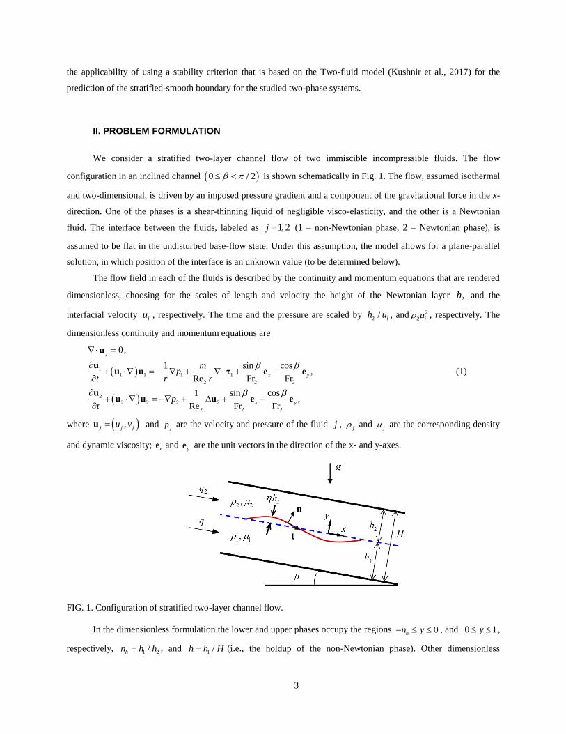


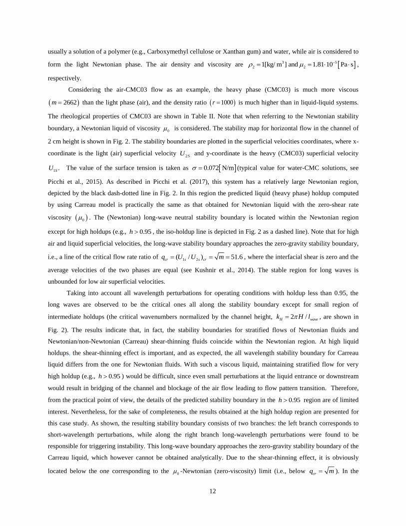


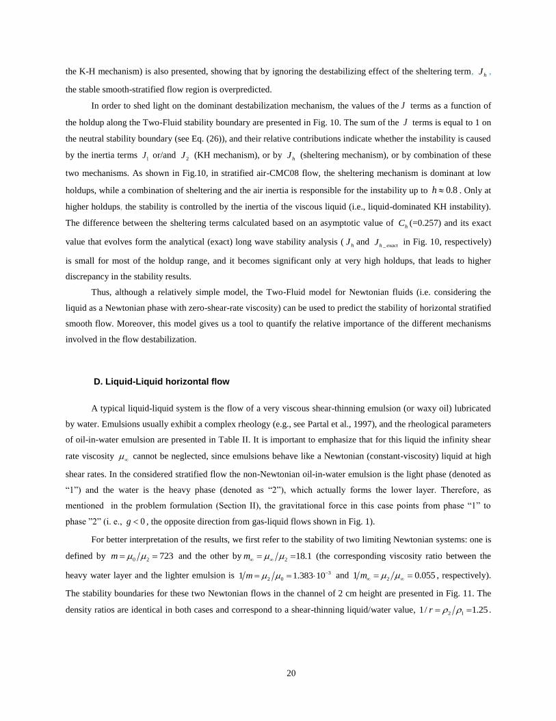


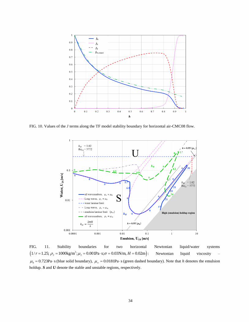


![Modelling of Stratified Mixture Flows, Heterogeneous Flows -Chapter 4- (Eb) [] [; ] {38s} #Ch 4 Unknown Book](https://static.documents.pub/doc/80x56/55cf8a9655034654898c0ee2/modelling-of-stratified-mixture-flows-heterogeneous-flows-chapter-4-eb.jpg)


