Stability of the Global Ocean Circulation: Basic...

Stability of the Global Ocean Circulation: Basic Bifurcation Diagrams

HENK A. DIJKSTRA

Institute for Marine and Atmospheric Research Utrecht, Utrecht University, Utrecht, Netherlands, and Department of AtmosphericScience, Colorado State University, Fort Collins, Colorado

WILBERT WEIJER

Scripps Institution of Oceanography, University of California, San Diego, La Jolla, California

(Manuscript received 4 April 2003, in final form 20 October 2004)

ABSTRACT

A study of the stability of the global ocean circulation is performed within a coarse-resolution generalcirculation model. Using techniques of numerical bifurcation theory, steady states of the global oceancirculation are explicitly calculated as parameters are varied. Under a freshwater flux forcing that isdiagnosed from a reference circulation with Levitus surface salinity fields, the global ocean circulation hasno multiple equilibria. It is shown how this unique-state regime transforms into a regime with multipleequilibria as the pattern of the freshwater flux is changed in the northern North Atlantic Ocean. In themultiple-equilibria regime, there are two branches of stable steady solutions: one with a strong northernoverturning in the Atlantic and one with hardly any northern overturning. Along the unstable branch thatconnects both stable solution branches (here for the first time computed for a global ocean model), thestrength of the southern sinking in the South Atlantic changes substantially. The existence of the multiple-equilibria regime critically depends on the spatial pattern of the freshwater flux field and explains thehysteresis behavior as found in many previous modeling studies.

1. Introduction

The response of the global ocean circulation tochanges in the surface buoyancy and wind forcing is oneof the important problems in climate research. The mo-mentum input through the wind stress is the main driv-ing mechanism of the flow in the upper layers of theocean, in particular for western boundary currents suchas the Gulf Stream, Kuroshio, and the Agulhas Cur-rent. The buoyancy input through the surface heat andfreshwater flux is crucial for the existence and structureof the stratification in the ocean and, hence, for themainly density-driven deep flow (Schmitz 1995).

A useful framework to understand the global circu-lation is the “Ocean Conveyor” (Gordon 1986). In thisview, the deep and surface flows in the Atlantic, Pacific,and Indian Ocean basins are connected through cur-rents in the Southern Ocean. The North Atlantic is oneof the central regions in this framework; here the north-ward flowing surface water becomes dense enoughto induce formation of North Atlantic Deep Water

(NADW). This water mass moves southward and canbe traced at depth far south in the Atlantic basin. Be-cause of the existence of this overturning branch of theAtlantic circulation, about 1.5 PW of heat is trans-ported northward at 24°N (Hall and Bryden 1982; Ga-nachaud and Wunsch 2000).

More and more evidence emerges that is in favor ofan active role of the ocean circulation in past climatechanges (Clark et al. 2002). The North Atlantic circu-lation has a special role because it appears sensitive tothe amplitude and pattern of the surface buoyancy forc-ing. There is much evidence that the freshwater input atparticular locations has caused, at several instances inthe geological past, a temporary slowdown of the NorthAtlantic circulation (Broecker 2000). A famous ex-ample is the onset of the Younger Dryas cooling event,about 12 000 years ago, which (likely) started with acatastrophic input of freshwater through diversion ofLake Agassiz from the Mississippi basin to the St.Lawrence drainage (Rooth 1982).

In addition, the response of the ocean circulation tochanges in the surface forcing is a central factor in thedifferent climate change scenarios computed with cur-rent climate models that investigate the impacts of in-creased atmospheric greenhouse gas concentrations(Houghton et al. 2001). The increased radiative forcing

Corresponding author address: Henk A. Dijkstra, Departmentof Atmospheric Science, Colorado State University, Fort Collins,CO 80526.E-mail: [email protected]

JUNE 2005 D I J K S T R A A N D W E I J E R 933

© 2005 American Meteorological Society

JPO2726

changes the hydrological cycle to induce more precipi-tation in the North Atlantic, which may slow down themeridional overturning circulation. Apart from changesin the freshwater flux, also changes in the ocean–atmosphere heat flux may affect the meridional over-turning. The degree of the slowdown depends on themodel configuration and on properties of the mean cli-mate state (Manabe and Stouffer 1999; Clark et al.2002).

Stability properties of the global ocean circulationhave first been addressed with ocean-only models. Thepioneering results of Bryan (1986) revived the interestin multiple flow patterns of the Atlantic Ocean circu-lation already suggested by Stommel (1961). One of theissues that has been extensively investigated is the sta-bility of the global ocean flow that arises under pre-scribed (observed) sea surface salinity (SSS) and seasurface temperature (SST) fields, with restoring timescales �S and �T, respectively. Tziperman et al. (1994)study the stability of these flows under mixed boundaryconditions (with a diagnosed freshwater flux) andfound that the circulation is unstable if �S is smallenough. In the latter case, the freshwater flux(evaporation�precipitation) becomes strongly negativein the northern North Atlantic, which inhibits northernsinking.

The sensitivity of the global ocean circulation tobuoyancy input into the North Atlantic has also beeninvestigated by adding freshwater at a very slow ratesuch that quasi-steady states are monitored in time(Rahmstorf 1995; Prange et al. 2002). In this way, a firstimpression of the stable equilibria of the global oceancirculation can be obtained (Rahmstorf 2000). In aglobal ocean general circulation model (OGCM)coupled to a zeroth-order atmosphere model, it isfound that when this freshwater input is strong enough,the Atlantic meridional overturning circulation (MOC)strongly decreases. When the freshwater forcing is re-versed from this weak MOC state, hysteresis behavioroccurs because this state can be maintained under sub-stantial negative freshwater flux (i.e., input of salt)anomalies. This has lead to the suggestion that the un-derlying bifurcation diagram is qualitatively similar tothat in the simple two-box model suggested in Stommel(1961).

Although there are models in which no weak MOCstate is found in the parameter regime investigated(Schiller et al. 1997), the multiple-equilibria structureappears to be a robust feature in coupled ocean–atmosphere models. Manabe and Stouffer (1999), forexample, showed that a weak MOC state is reached asa result of a certain freshwater perturbation in case theocean model has a small vertical mixing coefficient ofheat and salt that varies with depth. Note, however, thatwith a larger constant vertical mixing coefficient theMOC reduced substantially but recovered after sometime. Tziperman (1997) demonstrates that the occur-rence of a weak MOC state depends strongly on the

mean salinity field in the North Atlantic Ocean. Inthese model studies, the weak MOC state has deep-water formation in the Southern Ocean and upwellingin the northern North Atlantic.

The multiple-equilibria regime may be a very impor-tant characteristic of the global ocean circulation andlikely of the climate system. Its sensitivity to represen-tations of physical processes in ocean models is crucialto determine whether relatively rapid climate changes,as recorded in ice-core records (Alley et al. 1997), canbe attributed to changes in the global ocean circulation.It is also important for assessing the probability that afuture weakening of the MOC will occur as the concen-tration of greenhouse gases is increasing. Extensivesensitivity studies have only been performed in inter-mediate complexity models, such as zonally averagedmodels (Schmittner and Stocker 1999). Recently, Prahlet al. (2003) performed a sensitivity study of the hys-teresis behavior with respect to the vertical eddy diffu-sivity (KV) in a global ocean model. They show that thehysteresis behavior exists over a large range of values ofKV and that the width of the hysteresis loop becomessmaller with decreasing KV.

In this paper, the first explicit computation of thebifurcation diagram explaining the hysteresis behaviorof the global ocean circulation and its sensitivity to KV

is presented. The techniques of numerical bifurcationtheory are now in a stage that one is able to performthese computations for a low-resolution OGCM (4°horizontal resolution and 12 vertical layers) coupled toan energy-balance atmospheric model. For a similarconfiguration as used in Rahmstorf (1995), the com-plete bifurcation structure is computed including thebranch of unstable solutions, which is necessarilypresent in the bifurcation diagram. The connection toearlier bifurcation diagrams in more idealized configu-rations, that is, an Atlantic-only configuration, is pre-sented elsewhere (Dijkstra and Weijer 2003).

2. Model and methods

The behavior of the global ocean model described insection 2a is analyzed in a manner complementary totraditional model studies (Rahmstorf 1995; Tziperman,2000). The complementarity of the approach is de-scribed in section 2b using a simple example. In section2c, the numerical techniques are outlined and, as ex-plained in section 2d, they pose some restrictions on theparameter regime in the ocean model that can behandled.

a. Model

The description of the fully implicit global oceanmodel used in this study is presented in Weijer et al.(2003) to which the reader is referred for full details.The governing equations of the ocean model are thehydrostatic, primitive equations in spherical coordi-nates on a domain that includes full continental geom-

934 J O U R N A L O F P H Y S I C A L O C E A N O G R A P H Y VOLUME 35

etry as well as bottom topography. The ocean velocitiesin eastward and northward directions are indicated by uand �, the vertical velocity is indicated by w, the pres-sure by p, and the temperature and salinity by T and S.

The horizontal resolution of the model is about 4° [a96 � 38 grid in a domain (85.5°S–85.5°N, 0°–360° lon-gitudinally)], and the grid has 12 levels in the verticaldirection. The vertical grid is nonequidistant with themost upper (lowest) layer having a thickness of 50 m(1000 m), respectively. In the present version of theocean model, we have followed the configuration of theGeophysical Fluid Dynamics Laboratory (GFDL)Modular Ocean Model (MOM), as described in En-gland (1993) and used in Rahmstorf (1996), veryclosely. Vertical and horizontal mixing of momentumand heat/salt are represented by a Laplacian formula-tion with prescribed eddy viscosities AH and AV andeddy diffusivities KH and KV, respectively.

The oceanic flow is forced by the annual-mean windstress as given in Trenberth et al. (1989). The upperocean is coupled to a simple energy-balance atmo-spheric model as in Dijkstra et al. (2003), in which onlythe heat transport is modeled (no moisture transport);a short summary of this model is provided in the ap-pendix. The freshwater flux will be prescribed in eachof the results below. As in low-resolution OGCMs, thesurface forcing is represented as a body forcing over theupper layer. On the continental boundaries, no-slipconditions are prescribed, and the heat and salt fluxesare zero. At the bottom of the ocean, both the heat andsalt fluxes vanish and slip conditions are assumed.

b. Continuation methods

Since many readers may (still) be unfamiliar withcontinuation methods, a brief introduction into this ap-proach in relation to more traditional ocean modeling isgiven here.

Suppose one is interested in the changes of equilib-rium flows of a model (here the low-resolution globalocean model) with respect to changes in the forcingconditions, say the surface freshwater flux

FS � FS1 � �FS

2, �1�

where � [0, 1] is a parameter controlling the fresh-water flux (its pattern and amplitude) and the Fi

S (i �1, 2) are prescribed patterns.

In traditional ocean models, this problem would beapproached as a set of initial value problems for severalchosen values of , for example, � 0.25, 0.5, 0.75, and � 1.0. For the first value of , a motionless flow withinterpolated Levitus values for temperature and salinitycan be taken as an initial condition at time t � t0. Todetermine the equilibrium state, an initial value prob-lem is solved in which the solution at time t � tn�1 iscomputed from the solution at time t � tn.

To solve this initial value problem explicit techniquesare commonly used, such as leapfrog or Adams–

Bashforth. Mode splitting, where the barotropic modeis treated differently than the baroclinic modes, is oftenused, and sometimes the time steps for the tracers andmomentum are taken differently. In explicit methods,the time step is limited by numerical stability accordingto well-known criteria. After many time steps (a typicaltime step is 1 h and one has to integrate several thou-sands of years), one ends up with an equilibrium solu-tion for which all fields do not change in time anymore.Next, this procedure is repeated for the other values of. One could either choose the same initial conditionsas for the first value of or one can make use of equi-librium solutions computed at earlier values of .

As an example, consider the two-dimensional systemof differential equations given by

dx

dt� � � x2 and �2a�

dy

dt� x � y. �2b�

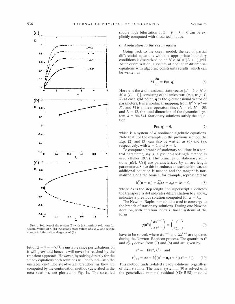
For each 0, when solved as an initial value problem,x(t) and y(t) are followed in time until a steady state isreached. If for these values of , x(t) is plotted versustime, a plot as in Fig. 1a results. However, for the ques-tion at hand, that is, the sensitivity of the equilibriaversus , only the end points of these calculations, say(x, y) � limt→�[x(t), y(t)], are of interest and typicallyone would show a plot as in Fig. 1b.

The continuation methods used here are designed todirectly compute the curve in Fig. 1b without goingthrough the transient calculations as in Fig. 1a. Insteadof solving the time-dependent equations, these tech-niques directly tackle the steady equations, that is, themodel equations with the time-derivatives put to zero.For the example,

� � x2 � 0 and �3a�

x � y � 0. �3b�

Solving directly for the latter has an important addi-tional advantage. For the steady states, we find x � y �� and x � y � �� for each value of 0. Look-ing at the evolution of small perturbations on thesestates, say

x � x � x and y � y � y, �4�

the linearized equations from (2) are

dx

dt� ��2x�x and �5a�

dy

dt� x � y. �5b�

For the solution x � y � �, the perturbations willdecay and hence the steady state is stable and will befound by transient integration (as in Fig. 1a). The so-


lution x � y � �� is unstable since perturbations onit will grow and hence it will never be reached by thetransient approach. However, by solving directly for thesteady equations both solutions will be found—also theunstable one! The steady-state branches, as they arecomputed by the continuation method (described in thenext section), are plotted in Fig. 1c. The so-called

saddle-node bifurcation at x � y � � 0 can be ex-plicitly computed with these techniques.

c. Application to the ocean model

Going back to the ocean model, the set of partialdifferential equations with the appropriate boundaryconditions is discretized on an N � M � (L � 1) grid.After discretization, a system of nonlinear differentialequations with algebraic constraints results, which canbe written as

Mdudt

� F�u, q�. �6�

Here u is the d-dimensional state vector [d � 6 � N �M � (L � 1)], consisting of the unknowns (u, �, w, p, T,S) at each grid point, q is the q-dimensional vector ofparameters, F is a nonlinear mapping from Rd � Rq →Rd, and M is a linear operator. Since N � 96, M � 38,and L � 12, the total dimension of the dynamical sys-tem, d � 284 544. Stationary solutions satisfy the equa-tion

F�u, q� � 0, �7�

which is a system of d nonlinear algebraic equations.Note that, for the example, in the previous section, theEqs. (2) and (3) can also be written as (6) and (7),respectively, with d � 2 and q � 1.

To compute a branch of stationary solutions in a con-trol parameter, say , a pseudo-arc-length method isused (Keller 1977). The branches of stationary solu-tions [u(s), (s)] are parameterized by an arc lengthparameter s. Since this introduces an extra unknown, anadditional equation is needed and the tangent is nor-malized along the branch, for example, represented by

u0T�u � u0� � �0

T�� 0� � �s � 0, �8�

where s is the step length, the superscript T denotesthe transpose, a dot indicates differentiation to s and u0

indicates a previous solution computed for � 0.The Newton–Raphson method is used to converge to

the branch of stationary solutions. During one Newtoniteration, with iteration index k, linear systems of theform

J�uk��uk�1

��k�1� � � rk

rd�1k � �9�

have to be solved, where uk�1 and k�1 are updatesduring the Newton–Raphson process. The quantities rk

and rkd�1 derive from (7) and (8) and are given by

rk � �F�uk, �k� and

rd�1k � �s � u0

T�uk � u0� � �0��k � �0�. �10�

This method finds isolated steady solutions, regardlessof their stability. The linear system in (9) is solved withthe generalized minimal residual (GMRES) method

FIG. 1. Solution of the system (2) with (a) transient solutions forseveral values of , (b) the steady-state values of x vs , and (c) thecomplete bifurcation diagram of (2).


(an iterative linear systems solver) using matrix renum-bered incomplete LU (MRILU) as a (multigrid-oriented) preconditioning technique. For details on thelatter methods, the reader is referred to Botta andWubs (1999) and Dijkstra et al. (2001).

The extended system of equations in (7)–(8) for theunknowns u(s) and (s) is needed to be able to followsolutions along saddle-node bifurcations. Rememberthat in the example (2), a saddle-node bifurcation oc-curred at x � y � � 0 where the Jacobian matrix from(5), that is,

J � ��2x 0

1 �1� �11�

becomes singular. This singularity would make it im-possible to use the Newton–Raphson method for thesystem (7). The extended system, with Jacobian J as in(9), is nonsingular, allowing one to trace branchesaround saddle-node bifurcations.

d. Shortcomings of the model

The GMRES and MRILU are sophisticated numeri-cal techniques enabling one to solve for a 284 544 sys-tem of nonlinear equations as arises from the discreti-zation of the ocean model [instead of a two-equationsystem as in (2)]. At the moment, there are two restric-tions under which this can be efficiently done for theglobal model: (i) a relatively large value of lateral eddyviscosity AH and (ii) a restriction on the use of convec-tive adjustment.

Many explicit ocean models of 4° resolution use typi-cal values of AH � 2.5 � 105 m2 s�1. If one considers themomentum equations in a single-hemispheric basin(Dijkstra et al. 2001), this value is far too small to re-solve the Ekman boundary layer near the eastern wall.This boundary layer has a thickness (AH/f0)1/2, where f0

� 2� sin�0 is the value of the Coriolis parameter atlatitude �0. General numerical practice is to resolvethese boundary layers since, otherwise, wiggles are en-countered.

When the implicit model is used to compute steadystates with this value of AH, wiggles are seen in thewhole solution. The discretization of the Coriolis termsprovides difficulties on the C grid because of the pres-ence of so-called velocity modes. The problem is exac-erbated in the implicit approach because the whole sys-tem of equations is solved simultaneously and there isno decoupling of barotropic and baroclinic modes. Inthe results below, we therefore restrict use to the C-gridcase in which the value of AH � 1.6 � 107 m2 s�1 is suchthat the lateral Ekman boundary layers are resolvedand lateral friction damps the velocity modes.

Convective adjustment is widely used in ocean mod-els and is easily implemented in explicit models, but itturns out to be difficult to use in implicit models. Themain difficulty is its nondifferentiable properties asso-ciated with an on/off behavior depending on the local

vertical density gradient. Local convective adjustmentmay lead to spurious equilibria (Vellinga 1998) whilethe global adjustment procedure (Dijkstra et al. 2001)cannot be used in a continuation setup. In most of theresults below we will not apply any convective adjust-ment scheme.

The resulting solutions appear “less realistic” thanthose of other ocean models with a comparable resolu-tion. However, they are the most “clean” solutions ofthe governing system of hydrostatic partial differentialequations in that boundary layers are well-resolved andno ad hoc procedures for convection have been applied.As will be shown below, the ocean flow is more slug-gish, but many characteristics are similar to equilibriumsolutions of traditional low-resolution ocean models(with the same spatial resolution).

3. Results

Starting from the trivial state, at zero solar forcing,no freshwater flux and no wind stress, first a branch ofequilibrium states is computed toward “realistic” forc-ing conditions. The latter consist of the annual-meanwind stress as in Trenberth et al. (1989), an analyticalform of the solar forcing as in the appendix, and theLevitus surface salinity distribution (Levitus et al.1994). The freshwater flux of this reference solution isdiagnosed and subsequently used as part of the surfacebuoyancy forcing. Next, a steady perturbation patternin the freshwater flux over a relatively small domain inthe North Atlantic is applied and the changes of theequilibrium flows with the amplitude of this perturba-tion are computed.

a. The unique regime

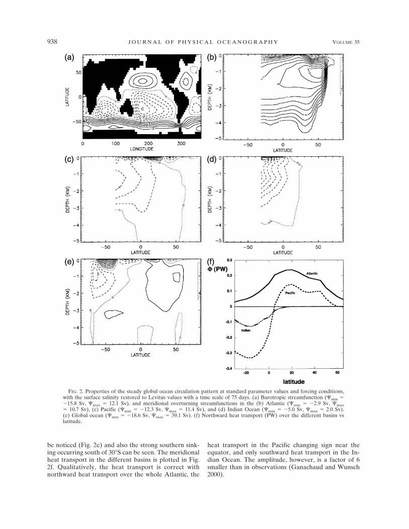
For the computation of the reference solution, a re-storing time scale of 75 days is used for the Levitussurface salinity. Standard values of eddy diffusivitiesare KV � 8 � 10�5 m2 s�1 and KH � 103 m2 s�1 and thevertical eddy viscosity AV � 10�3 m2 s�1. The proper-ties of the reference steady state are plotted in Fig. 2. Inthe barotropic streamfunction (Fig. 2a), the gyre struc-ture can be seen in each basin together with the Ant-arctic Circumpolar Current (ACC). The maximum vol-ume transport of the ACC is about 12 Sv (Sv � 106

m3 s�1), the latter due to the relatively large value ofAH. The maximum of the Atlantic meridional overturn-ing streamfunction (Fig. 2b) is about 11 Sv, which isslightly smaller than in other models (England 1993).One of the factors causing the smaller overturning isthe absence of convective adjustment. The meridionaloverturning in the Pacific Ocean (Fig. 2c) and the In-dian Ocean (Fig. 2d) is relatively strong with extremesof about �12 and �5 Sv, respectively. In all threeoceans, there are Ekman driven surface circulation cellshaving a relatively small amplitude of a few Sverdrups.In the global overturning streamfunction, the ACC can


be noticed (Fig. 2e) and also the strong southern sink-ing occurring south of 30°S can be seen. The meridionalheat transport in the different basins is plotted in Fig.2f. Qualitatively, the heat transport is correct withnorthward heat transport over the whole Atlantic, the

heat transport in the Pacific changing sign near theequator, and only southward heat transport in the In-dian Ocean. The amplitude, however, is a factor of 6smaller than in observations (Ganachaud and Wunsch2000).

FIG. 2. Properties of the steady global ocean circulation pattern at standard parameter values and forcing conditions,with the surface salinity restored to Levitus values with a time scale of 75 days. (a) Barotropic streamfunction (�min ��15.8 Sv, �max � 12.1 Sv), and meridional overturning streamfunctions in the (b) Atlantic (�min � �2.9 Sv, �max� 10.7 Sv), (c) Pacific (�min � �12.3 Sv, �max � 11.4 Sv), and (d) Indian Ocean (�min � �5.0 Sv, �max � 2.0 Sv).(e) Global ocean (�min � �18.6 Sv, �max � 39.1 Sv). (f) Northward heat transport (PW) over the different basins vslatitude.


Although many details of this equilibrium solutionare incorrect when compared with observations, theoverall characteristics of the flow are adequate and,apart from the weaker barotropic transport, compa-rable to those in other global OGCMs (Manabe andStouffer 1988; Tziperman et al. 1994; Rahmstorf 1995)using the same (very coarse) resolution. For example,in Manabe and Stouffer (1988), a meridional heat trans-port of about 0.5 PW is found at 24°N in the Atlanticand other models find similar values. The flow here issimply more sluggish than in the other models becauseof the larger value of AH and the absence of convectiveadjustment. This leads to the smaller values of the heattransport found. Apart from this, many characteristics(such as the heat transport) are qualitatively correct.

Next, the freshwater flux is diagnosed from this ref-erence solution; this flux (Fig. 3b) is needed to maintainthe (interpolated) Levitus surface salt field (shown inFig. 3a) with the steady state reference flow. Largestamplitudes, with typical values of 3.8 m yr�1, occur overthe southern Indian Ocean and in the northern NorthAtlantic. Although the freshwater flux differs substan-tially from the observation based annual mean field

(Oberhuber 1988), the pattern is just as noisy as thosediagnosed in other OGCMs using the same resolution(Tziperman et al. 1994) and the large amplitude fea-tures roughly correspond. For example, in the NorthAtlantic, there is a zonal dipolar structure with largeamplitude that can also be seen in Fig. 2 of Tzipermanet al. (1994). The salt input in the positive part of thisdipole near 40°N is needed to compensate for the mod-el’s incorrect representation of the salt transport due tothe Gulf Stream.

In Weaver and Hughes (1996), the same dipolarstructure in the freshwater flux is found near otherwestern boundary currents, such as the Kuroshio andAgulhas. These dipoles are neither found here nor inTziperman et al. (1994). The reason for this differenceis probably the higher horizontal resolution (about 2°)in the Weaver and Hughes (1996) model. In the inter-polation of the Levitus salinity field in the presentmodel, there is hardly any zonal salt gradient in theKuroshio region. On a higher resolution, this would bethe case and hence a compensating effect of the fresh-water flux, because of the misrepresentation of the Kuro-shio salt transport (as in the Gulf Stream), is required.

FIG. 3. (a) Surface salinity anomaly with respect to S0 � 35 psu, with Smin � �4.7 psu and Smax � 2.2 psu. (b) Diagnosedfreshwater flux field (in units of 10�8 m s�1) of the state in Fig. 2. The minimum and maximum values are �15.8 � 10�8

m s�1 and 12.5 � 10�8 m s�1, respectively. (c) Basin averaged freshwater flux. (d) Northward freshwater transport.


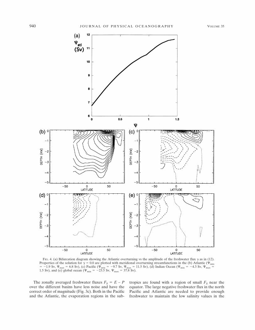
The zonally averaged freshwater fluxes FS � E – Pover the different basins have less noise and have thecorrect order of magnitude (Fig. 3c). Both in the Pacificand the Atlantic, the evaporation regions in the sub-

tropics are found with a region of small FS near theequator. The large negative freshwater flux in the northPacific and Atlantic are needed to provide enoughfreshwater to maintain the low salinity values in the

FIG. 4. (a) Bifurcation diagram showing the Atlantic overturning vs the amplitude of the freshwater flux � as in (12).Properties of the solution for � � 0.0 are plotted with meridional overturning streamfunctions in the (b) Atlantic (�min� �1.9 Sv, �max � 6.8 Sv), (c) Pacific (�min � �9.7 Sv, �max � 11.5 Sv), (d) Indian Ocean (�min � �4.3 Sv, �max �1.5 Sv), and (e) global ocean (�min � �23.5 Sv, �max � 37.8 Sv).


Levitus dataset (Fig. 3a). The meridional freshwatertransport in the different basins is shown in Fig. 3d.Although these are not well known from observations,the values here are about a factor of 6 smaller thancurrent estimates (Wijffels et al. 1992). Although thesign of the freshwater transport is correct in the NorthAtlantic, it is not in the North Pacific. These modelerrors are well known from traditional OGCMs andhave to be accepted at this low resolution.

In many previous bifurcation studies of thermohalinedriven flows [see chapter 6 in Dijkstra (2000)], thestructure of steady solutions was investigated with thestrength of the freshwater flux as control parameter,while keeping its pattern fixed. If the freshwater fluxfield in Fig. 3b is indicated by F1

S(�, �), then the surfacefreshwater flux FS is prescribed as

FS � �FS1��, ��, �12�

where � is a dimensionless amplitude. The bifurcationdiagram showing the maximum of the Atlantic meridi-onal overturning streamfunction �atl versus � is plottedin Fig. 4. The value of �atl increases monotonically with� from about 6.8 Sv at � � 0.0 up to about 11.5 Sv at� � 1.5.

Properties of the thermally only driven solution (for� � 0.0) are shown in the Figs. 4b–e. Note that for thissolution, the salinity is homogeneous over the globalocean. In Fig. 2b, about 75% of the North AtlanticDeep Water leaves the Atlantic at the southern bound-ary. This amount has decreased to about 30% in Fig. 4bas nearly all the deep water reaches the surface before30°S. The overturning extends slightly more northwardthan that of the reference solution. This is because ofthe freshwater input in the northern North Atlantic(Fig. 3b) present in the forcing of the reference solu-tion.

The southern overturning cell in the Pacific (Fig. 4c)becomes slightly weaker (it has changed to �9.7 Sv),and there is now even a northern overturning cell ofabout 4 Sv. The strong freshwater input in the NorthPacific (Fig. 3b) inhibits the presence of this northernoverturning cell in the reference solution. The over-turning streamfunction in the Indian Ocean (Fig. 4d)and the global barotropic streamfunction (not shown)are hardly affected. In the global meridional overturn-ing streamfunction (Fig. 4e) the amplitude of the south-ern sinking cell has increased to about 20 Sv.

It is clear that each equilibrium of the global oceancirculation is unique for a fixed value of � (Fig. 4a). Ifa transient simulation would be started from the refer-ence equilibrium solution (� � 1) it would remain nearthat state under the prescribed freshwater flux, similarto the large �S results in Tziperman et al. (1994).

b. The multiple-equilibria regime

We first define a region near Newfoundland, similarto region A in Rahmstorf (1995), with domain (�, �) ∈

[60°–24°W] � [54°–66°N]. To study the impact ofchanges in the freshwater flux pattern, a perturbationflux Fp

S is defined as

FSp � �pFS

2��, ��, �13�

where F2S(�, �) � 1 in the region near Newfoundland

and zero outside. The value of �p controls the ampli-tude of the freshwater flux perturbation, and followingprevious model studies, it will be expressed in Sver-drups. When changing �p, one has to take care that thesalt balance is closed; that is, we subtract the surface-integrated value Q from the total freshwater flux pro-file, such that

FIG. 5. (a) Bifurcation diagram of the steady states of the globalocean circulation as a plot of the maximum meridional Atlanticoverturning vs the anomalous freshwater-flux strength �p (Sv).Note that for �p � 0, the reference solution is obtained. (b)Changes in the Atlantic meridional heat transport along the curvein (a).


1|S | �S

�FS1��, �� pFS

2��, �� r02 cos� d� d� � Q � 0,

�14�

where |S | is the total area of the ocean surface.The bifurcation diagram, showing the maximum At-

lantic meridional overturning of the steady solutionsversus �p is plotted in Fig. 5a. It consists of two saddle-node bifurcations, indicated by L1 (�p � �0.18 Sv) andL2 (�p � �0.052 Sv), that exactly bound the regime ofmultiple equilibria of these flows. Stable solutions areindicated by a continuous line style while the branchof unstable solutions is dashed. From the reference so-lution (�p � 0.0) in this model configuration (Fig. 2),one needs to increase the amplitude of the freshwaterflux perturbation beyond �p � �0.052 Sv to reach intothe multiple-equilibria regime. In this regime, a transi-tion to a weak Atlantic MOC state can occur. For val-ues smaller than �p � �0.18 Sv, only the latter stateexists.

The changes in the Atlantic meridional heat trans-port along the equilibrium curve are plotted in Fig. 5b.The labels refer to solutions marked at specific loca-tions in Fig. 5a. At point B, the heat transport is stillpositive over the Atlantic, but along the unstable

branch (point C) the heat transport changes sign in theSouth Atlantic. In the weak MOC state, the heat trans-port is qualitatively similar to that Pacific in the refer-ence solution (Fig. 2f). This behavior of the heat trans-port is consistent with the decrease in meridional over-turning as found in Fig. 5a.

With decreasing �p, starting from the reference solu-tion, the Atlantic overturning decreases until thesaddle-node bifurcation L1 at �p � �0.18 Sv. Note thatthe equilibrium states on this branch are still linearlystable in the multiple equilibrium regime (�0.18 Sv ��p � �0.052 Sv). Hence, when a transient computationis started from an initial condition that is only a smallperturbation of the equilibrium state (e.g., by a smallchange in the freshwater input over a certain region), itwill return to the equilibrium state. A finite-amplitudeperturbation is therefore needed to induce a transitionto the stable weak MOC state on the lower branch inFig. 5a and whether a transition will occur depends onthe amplitude of this perturbation. Note that, becausethe steady states change with �p, also the critical am-plitude of this finite-amplitude perturbation changeswith �p.

The solution near the saddle-node bifurcation L1 inFig. 5a is shown in Fig. 6. The surface salinity field inthe Atlantic (not shown) has decreased by about 1 psu

FIG. 6. Properties of the steady global ocean circulation pattern at the saddle-node bifurcation L1 in Fig. 5. Meridionaloverturning streamfunction: (a) global ocean (�min � �22.1 Sv, �max � 38.5 Sv), (b) Atlantic (�min � �2.7 Sv, �max �6.4 Sv), (c) Pacific (�min � �12.4 Sv, �max � 11.5 Sv), and (d) Indian Ocean (�min � �5.1 Sv, �max � 1.9 Sv).


with respect to that of the reference solution. In theglobal overturning streamfunction (Fig. 6a), the south-ern overturning in the region south of the 30° has in-creased with respect to that of the reference solutionand the northern overturning in the Northern Hemi-sphere has weakened. Only the changes in the Atlanticoverturning (Fig. 6b) contribute to this (it has weak-ened) as the overturning circulation in the other basinsis hardly affected (Figs. 6b,c). This indicates a fairlylocalized response of the equilibrium circulation to thelocal anomalous freshwater flux. In the North Atlantic,the latitude of sinking has slightly moved southwardwith respect to the reference solution and there is asmall amount of bottom water at depth. The upwellingof deep water has also increased since the streamlinesin (Fig. 6a) are tilted upward to the south.

Along the unstable (dashed) branch in Fig. 5a, theAtlantic overturning strength of the northern sinkingsolution seems to remain fairly constant. However, thisis a consequence of the norm chosen since it is deter-mined by the wind-driven Ekman cell at the surface.Actually, it is along this branch that the solution totallychanges character: northern sinking is inhibited and thevolume of bottom water coming from the south in-creases. Last, the northern sinking cell in the Atlantic

has basically disappeared, while the southern sinkingcell has increased in amplitude to an overturningstrength of about �4 Sv at the saddle-node bifurcationL2 at �p � �0.052 Sv.

The solution at this saddle-node bifurcation is shownin Fig. 7. There is only a slight region in the subtropicalAtlantic where the salinity is larger than 35 psu. Thesinking in the Southern Hemisphere has increased by 5Sv (Fig. 7a), but the pattern of the global overturning isfairly similar to that in Fig. 6a. There is still a smallsubsurface sinking with a maximum of about 5 Sv in theNorth Atlantic (Fig. 7b) but, otherwise, sinking onlyoccurs in the Southern Ocean. Again, the whole reor-ganization of the Atlantic overturning pattern hashardly any influence on the flows in the Pacific andIndian Ocean (Figs. 7c,d). The maximum Indian Oceanmeridional overturning has only changed by about 1%along the whole unstable branch (and the maximumPacific overturning even less).

Along the lower branch (lower continuous line seg-ment in Fig. 5a), the Atlantic overturning decreaseswith increasing freshwater input (more negative �p).The solution in Fig. 8 shows the southern sinking (weakMOC) state at a quite large negative value of �p ��0.42 Sv. The sea surface salinity field now shows a

FIG. 7. Properties of the steady global ocean circulation pattern at the saddle-node bifurcation L2 in Fig. 5. Meridionaloverturning streamfunction: (a) global (�min � �27.3 Sv, �max � 37.6 Sv), (b) Atlantic (�min � �3.9 Sv, �max � 5.0 Sv),(c) Pacific (�min � �12.4 Sv, �max � 11.4 Sv), and (d) Indian Ocean (�min � �5.1 Sv, �max � 1.8 Sv).


very strong negative anomaly of about 10 psu in theNorth Atlantic and in nearly all of the Atlantic, thesalinity is lower than 35 psu. While the global meridi-onal overturning has not changed much (Fig. 8a), themaximum of southern overturning in the Atlantic hasshifted upward such that the Ekman cells are nowhardly visible (Fig. 8b). In the Pacific and IndianOcean, the salinity has increased because of the con-straint (14). It is due to these changes in the salinityfield that the overturning in Pacific and Indian Ocean(Figs. 8c,d) is also affected and both show a 10% in-crease in southern overturning with respect to the so-lution at L2.

c. Sensitivity to KV

From studies with global ocean models, it is foundthat the hysteresis behavior depends on the verticalmixing coefficient. For example, Prahl et al. (2003) find,by varying the surface values of the vertical mixing co-efficient KV, that the hysteresis does exist over a largerange of KV. For small values of KV the hysteresis in-terval decreases with decreasing values of KV and itfinally seems to disappear.

In the quasi-equilibrium computations with OGCMs,the multiple-equilibria regime has to be estimated from

the hysteresis loop. This is not trivial since, even beforethe saddle-node bifurcation is reached, the equilibriumsolution already reacts to the quasi-steady freshwaterchanges. Complementary to the quasi-equilibrium com-putations, the results here provide the exact location ofthe saddle-node bifurcations (L1 and L2 in Fig. 5a).Hence, by following the �p position of the saddle-nodebifurcations in KV, a regime diagram in the two-parameter (�p, KV) plane is obtained. This regime dia-gram exactly shows the sensitivity of the multiple-equilibria regime to KV.

Bifurcation diagrams for the smallest and largest val-ues of KV used are plotted in Fig. 9a. The topologicalshape of the diagrams is similar and for both cases, thedouble saddle-node structure is found. The distance in�p between the saddle-node bifurcations decreasesslightly with KV, as can also be seen in the regime dia-gram plotted in Fig. 9b over the range of 8.0 � 10�5 �KV � 10�3 m2 s�1. Note that the fact that one of thesaddle-node bifurcations for KV � 10�3 is located onthe curve for KV � 8 � 10�5 does not mean anything;it is just because of the choice of norm.

Our results are qualitatively similar to those in Prahlet al. (2003) although the procedure used is slightlydifferent. While they use the same freshwater flux for

FIG. 8. Properties of the steady global ocean circulation pattern at the left endpoint of the branch in Fig. 5 at �p � �0.42Sv. Meridional overturning streamfunction: (a) global ocean (�min � �28.7 Sv, �max � 36.1 Sv), (b) Atlantic (�min ��8.3 Sv, �max � 2.9 Sv), (c) Pacific (�min � �12.0 Sv, �max � 12.4 Sv), and (d) Indian Ocean (�min � �5.7 Sv, �max� 1.3 Sv).


each value of KV, we use the diagnosed freshwater fluxobtained from the restoring solution at each value ofKV. Hence, in our case, the diagnosed flux is able tomaintain the Levitus surface salinity distribution at �p

� 0. The fact that no hysteresis is found at very smallvalues of KV in Prahl et al. (2003) is probably due tofact that the freshwater flux they use can only sustainthe weak MOC solution (for all values of �p) and hencea unique solution exists.

4. Summary and discussion

For the first time, explicit bifurcation diagrams of theglobal ocean circulation have been calculated for a low-

resolution OGCM by techniques from dynamical sys-tems theory. For a configuration and parameter setupchosen quite similar to those in England (1993) andRahmstorf (1995) except for the large lateral viscosity,which makes the flow more sluggish, steady ocean cir-culation patterns are determined in parameter space.Without the computation of a single transient flow,both unique and multiple-equilibria regimes are found.For the standard configuration, it turns out that thereare no multiple equilibria of the global ocean circula-tion under a freshwater flux, which is diagnosed fromthe Levitus surface salinity field. Multiple equilibriaonly appear when the northern North Atlantic Ocean isfreshened. In that case, in addition to the northern sink-ing equilibrium, a solution with southern sinking is alsodynamically possible.

Previous model studies have shown indications thatthe location of the hysteresis regime depends on vari-ous processes, such as vertical mixing (Manabe andStouffer, 1999) and the restoring time scale of salinity inthe reference solution of Tziperman et al. (1994), whichare assumed constant in the present study. The tech-niques to compute equilibria of large-dimensional dy-namical systems, here with a dimension of about280 000, allow us to determine systematically the sen-sitivity of the global ocean circulation to the strengthand representation of the various large-scale processes.Although this work is still in progress, some scenarioscan already be anticipated.

For example, because of the different restoring timescale for salinity in the results by Tziperman et al.(1994) different equilibrium points within the diagramare reached. Their equilibrium computed with thesmaller value of �S experiences an additional freshwaterflux into the North Atlantic as compared with theirreference solution. A decreasing value of �S is thereforemimicked in the model here as a more negative value of�p. Indeed, the latter promotes the multiple-equilibriaregime as is seen in Fig. 5a. While for large �S, it isdifficult to determine whether the equilibrium is in theunique or multiple-equilibria regime, the solution forsmall �S is certainly in the multiple-equilibria regimebecause it is unstable according to Tziperman et al.(1994); hence it must be located on the unstable branch.A similar view may apply to the results of Manabe andStouffer (1999) where a larger value of the vertical mix-ing coefficient of heat and salt likely shifts the oceanstate from the multiple equilibria into the unique re-gime.

The existence of the multiple-equilibria regime isnot critically dependent on convective adjustment,since it is here also found in a model in which thisprocedure is not applied. Omitting this procedure haslead to a smooth single branch in Fig. 5a instead of thehighly variable temporal signature as found in quasi-equilibrium simulations (Rahmstorf 1995). Convectiveadjustment makes the equilibria very sensitive to localfinite-amplitude perturbations, which results in excur-

FIG. 9. (a) Bifurcation diagrams for two values of KV as curvesof the maximum Atlantic meridional overturning vs the strengthof the anomalous freshwater flux �p. (b) Regime diagram in thetwo-parameter (�p, KV) plane.


sions to nearby local equilibria in a quasi-equilibriumsimulation (Vellinga 1998). The multiple-equilibria re-gime is shown here to be fairly robust to changes in KV

similar to results in traditional ocean models (Prahl etal. 2003).

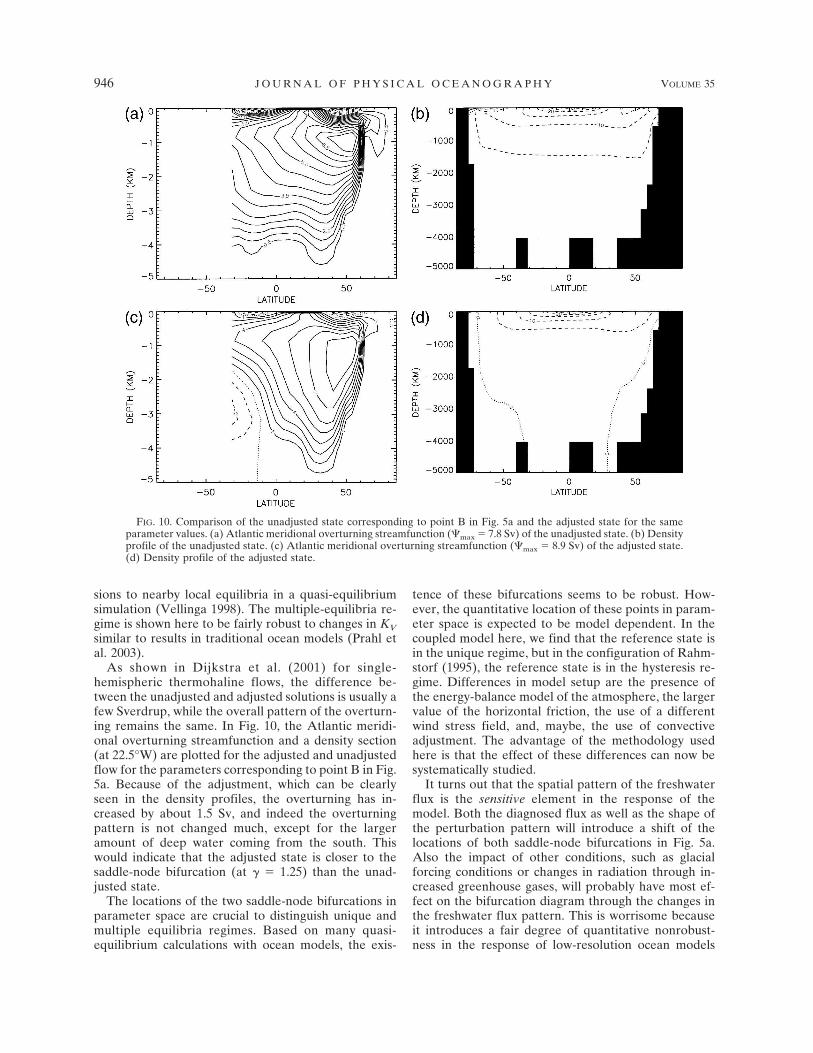
As shown in Dijkstra et al. (2001) for single-hemispheric thermohaline flows, the difference be-tween the unadjusted and adjusted solutions is usually afew Sverdrup, while the overall pattern of the overturn-ing remains the same. In Fig. 10, the Atlantic meridi-onal overturning streamfunction and a density section(at 22.5°W) are plotted for the adjusted and unadjustedflow for the parameters corresponding to point B in Fig.5a. Because of the adjustment, which can be clearlyseen in the density profiles, the overturning has in-creased by about 1.5 Sv, and indeed the overturningpattern is not changed much, except for the largeramount of deep water coming from the south. Thiswould indicate that the adjusted state is closer to thesaddle-node bifurcation (at � � 1.25) than the unad-justed state.

The locations of the two saddle-node bifurcations inparameter space are crucial to distinguish unique andmultiple equilibria regimes. Based on many quasi-equilibrium calculations with ocean models, the exis-

tence of these bifurcations seems to be robust. How-ever, the quantitative location of these points in param-eter space is expected to be model dependent. In thecoupled model here, we find that the reference state isin the unique regime, but in the configuration of Rahm-storf (1995), the reference state is in the hysteresis re-gime. Differences in model setup are the presence ofthe energy-balance model of the atmosphere, the largervalue of the horizontal friction, the use of a differentwind stress field, and, maybe, the use of convectiveadjustment. The advantage of the methodology usedhere is that the effect of these differences can now besystematically studied.

It turns out that the spatial pattern of the freshwaterflux is the sensitive element in the response of themodel. Both the diagnosed flux as well as the shape ofthe perturbation pattern will introduce a shift of thelocations of both saddle-node bifurcations in Fig. 5a.Also the impact of other conditions, such as glacialforcing conditions or changes in radiation through in-creased greenhouse gases, will probably have most ef-fect on the bifurcation diagram through the changes inthe freshwater flux pattern. This is worrisome becauseit introduces a fair degree of quantitative nonrobust-ness in the response of low-resolution ocean models

FIG. 10. Comparison of the unadjusted state corresponding to point B in Fig. 5a and the adjusted state for the sameparameter values. (a) Atlantic meridional overturning streamfunction (�max � 7.8 Sv) of the unadjusted state. (b) Densityprofile of the unadjusted state. (c) Atlantic meridional overturning streamfunction (�max � 8.9 Sv) of the adjusted state.(d) Density profile of the adjusted state.


that are often used as components in climate models.The spatial pattern of the freshwater flux is very diffi-cult to determine in the latter models with an atmo-spheric component that captures only large-scale pro-cesses. In model–model intercomparisons, patterns ofthe freshwater flux will differ widely and hence theircorresponding ocean equilibrium solutions, with largestdifferences in the North Atlantic. This quantitativenonrobustness is certainly undesired in studies assess-ing the effect of increasing atmospheric greenhouse gasconcentrations (Houghton et al. 2001).

Acknowledgments. This work was supported by theNetherlands Organization for Scientific Research(NWO) under a PIONIER grant to HD. We thank oneof the anonymous reviewers for the helpful commentson the manuscript, which lead to a much improved pa-per. All computations were done on the Origin 3800computer at SARA Amsterdam. Use of these comput-ing facilities was sponsored by the National ComputingFacilities Foundation (N.C.F.) under Project SC029with financial support from NWO.

APPENDIX

Atmospheric Energy Balance Model

The atmospheric model used is one of the simplestversions of the class of energy-balance models (Northet al. 1981). The freshwater flux is prescribed instead ofbeing determined from a moisture budget equation.The equation for the atmospheric surface temperatureTa on the global domain is given by

�aHaCpa

�Ta

�t� �aHaCpaD0��D��Ta� � �A � BTa�

�0

4S��1 � ��1 � C0�

� �oa�1 � L��T � Ta� � �laL�Tl � Ta�,

�A1�

where �a � 1.25 kg m�3 is the atmospheric density, Cpa

� 103 J (kg K)�1 is the heat capacity, � � 0.3 is theconstant albedo, Ha � 8.4 � 103 m is an atmosphericscale height, �0 � 1.36 � 103 W m�2 is the solar con-stant, D0 � 3.1 � 106 m2 s�1 is a constant eddy diffu-sivity, and 1 � C0 � 0.57 is the atmospheric absorptioncoefficient. The functions D(�) and S(�) give the lati-tude dependence of the eddy diffusivity and the short-wave radiative heat flux with

D�� 0.9 � 1.5 exp��12�2

�� and

S�� 1 �12

�0.482�3 sin��2 � 1�. �A2�

The constants A � 216 W m�2 and B � 1.5 W m�2 K�1

control the magnitude of the longwave radiative flux.

Last, T is the sea surface temperature, Tl the tem-perature of the land surface points, and the coefficientL indicates whether the underlying surface is ocean (L� 0) or land (L � 1). The exchange of heat betweenatmosphere and ocean and between atmosphere andthe land surface is modeled by constant exchange co-efficients. We assume here for simplicity that both areequal, with

�la � �oa � �aCpaCH |Va | � �, �A3�

where CH � 1.22 � 10�3 and |Va | � 8.5 m s�1 is a meanatmospheric surface wind speed; it follows that � � 13W m�2 K�1.

Boundary conditions for the atmosphere are periodicin zonal direction and no-flux conditions at the north–south boundaries; that is,

Ta�� W� � Ta�� E�;

�Ta

�� W� �

�Ta

�� E� �A4a�

� � ��S, �N :�Ta

�� 0. �A4b�

The net downward heat flux into the ocean and land isgiven by

Qoa �0

4S��1 � �C0 � ��T � Ta� �A5a�

and

Qla �0

4S��1 � �C0 � ��Tl � Ta�. �A5b�

When the heat capacity of the land is assumed to bezero, then Qla � 0 and the land temperature Tl is com-puted directly from

Tl � Ta ��0

4�S��1 � �C0. �A6�

In this way, the following integral conditions are satis-fied in steady state

�S

Qoa�1 � L� d2x � 0 �A7a�

and

�S��0

4S��1 � � � �A � BTa�� d2x � 0, �A7b�

with the integral

�S

d2x � ��W

�E ��S

�N

r02 cos� d� d�. �A8�

From the last integral condition it follows that the av-erage atmospheric temperature is independent of theland–sea distribution.


REFERENCES

Alley, R. B., P. A. Mayewski, T. Sowers, M. Stuiver, K. C. Taylor,and P. A. Clark, 1997: Holocene climate variability: A promi-nent widespread event 8200 years ago. Geology, 25, 483–486.

Botta, E. F. F., and F. W. Wubs, 1999: MRILU: An effectivealgebraic multilevel ILU-preconditioner for sparse matrices.SIAM J. Matrix Anal. Appl., 20, 1007–1026.

Broecker, W. S., 2000: Abrupt climate change: Causal constraintsprovided by the paleoclimate record. Earth-Sci. Rev., 51, 137–154.

Bryan, F. O., 1986: High-latitude salinity effects and interhemi-spheric thermohaline circulations. Nature, 323, 301–304.

Clark, P. U., N. G. Pisias, T. F. Stocker, and A. J. Weaver, 2002:The role of the thermohaline circulation in abrupt climatechange. Nature, 415, 863–869.

Dijkstra, H. A., 2000: Nonlinear Physical Oceanography: A Dy-namical Systems Approach to the Large Scale Ocean Circu-lation and El Niño. Kluwer Academic, 456 pp.

——, and W. Weijer, 2003: Stability of the global ocean circula-tion: The connection of equilibria in a hierarchy of models. J.Mar. Res., 61, 725–743.

——, H. Öksüzoglu, F. W. Wubs, and E. F. F. Botta, 2001: A fullyimplicit model of the three-dimensional thermohaline oceancirculation. J. Comput. Phys., 173, 685–715.

——, W. Weijer, and J. D. Neelin, 2003: Imperfections of thethree-dimensional thermohaline ocean circulation: Hyster-esis and unique state regimes. J. Phys. Oceanogr., 33, 2796–2814.

England, M. H., 1993: Representing the global-scale water massesin ocean general circulations models. J. Phys. Oceanogr., 23,1523–1552.

Ganachaud, A., and C. Wunsch, 2000: Improved estimates ofglobal ocean circulation, heat transport and mixing from hy-drographic data. Nature, 408, 453–457.

Gordon, A. L., 1986: Interocean exchange of thermocline water. J.Geophys. Res., 91, 5037–5046.

Hall, M., and H. Bryden, 1982: Direct estimates of ocean heattransport. Deep-Sea Res., 29, 339–359.

Houghton, J. T., Y. Ding, D. J. Griggs, M. Noguer, P. J. van derLinden, X. Dai, K. Maskell, and C. A. Johnson, Eds., 2001:Climate Change 2001: The Scientific Basis. Cambridge Uni-versity Press, 881 pp.

Keller, H. B., 1977: Numerical solution of bifurcation and nonlin-ear eigenvalue problems. Applications of Bifurcation Theory,P. H. Rabinowitz, Ed., Academic Press, 359–385.

Levitus, S., R. Burgett, and T. Boyer, 1994: Salinity. Vol. 3, WorldOcean Atlas 1994, NOAA Atlas NESDIS 3, 99 pp.

Manabe, S., and R. J. Stouffer, 1988: Two stable equilibria of acoupled ocean–atmosphere model. J. Climate, 1, 841–866.

——, and ——, 1999: Are two modes of thermohaline circulationstable? Tellus, 51A, 400–411.

North, G. R., R. F. Cahalan, and J. A. Coakley, 1981: Energybalance climate models. Rev. Geophys. Space Phys., 19, 19–121.

Oberhuber, J. M., 1988: The budget of heat, buoyancy and tur-bulent kinetic energy at the surface of the Global Ocean. MaxPlanck Institute für Meteorologie Hamburg Rep. 15, 148 pp.

Prahl, M., G. Lohmann, and A. Paul, 2003: Influence of verticalmixing on the thermohaline hysteresis: Analysis of an OGCM.J. Phys. Oceanogr., 33, 1707–1721.

Prange, M., V. Romanova, and G. Lohmann, 2002: The glacialthermohaline circulation: Stable or unstable? Geophys. Res.Lett., 29, 1–4.

Rahmstorf, S., 1995: Bifurcations of the Atlantic thermohalinecirculation in response to changes in the hydrological cycle.Nature, 378, 145–149.

——, 1996: On the freshwater forcing and transport of the Atlan-tic thermohaline circulation. Climate Dyn., 12, 799–811.

——, 2000: The thermohaline circulation: A system with danger-ous thresholds? Climate Change, 46, 247–256.

Rooth, C., 1982: Hydrology and ocean circulation. Progress inOceanography, Vol. 11, Pergamon, 131–149.

Schiller, A., U. Mikolajewicz, and R. Voss, 1997: The stability ofthe North Atlantic thermohaline circulation in a coupledocean-atmosphere general circulation model. Climate Dyn.,13, 325–347.

Schmittner, A., and T. F. Stocker, 1999: The stability of the ther-mohaline circulation in global warming experiments. J. Cli-mate, 12, 1117–1133.

Schmitz, W. J., 1995: On the interbasin-scale thermohaline circu-lation. Rev. Geophys., 33, 151–173.

Stommel, H., 1961: Thermohaline convection with two stable re-gimes of flow. Tellus, 2, 224–230.

Trenberth, K. E., J. G. Olson, and W. G. Large, 1989: A globalocean wind stress climatology based on ECMWF analyses.National Center for Atmospheric Research Tech. Rep.NCAR/TN-338�STR, 93 pp.

Tziperman, E., 1997: Inherently unstable climate behavior due toweak thermohaline ocean circulation. Nature, 386, 592–595.

——, 2000: Proximity of the present-day thermohaline circulationto an instability threshold. J. Phys. Oceanogr., 30, 90–104.

——, J. R. Toggweiler, Y. Feliks, and K. Bryan, 1994: Instabilityof the thermohaline circulation with respect to mixed bound-ary conditions: Is it really a problem for realistic models? J.Phys. Oceanogr., 24, 217–232.

Vellinga, M., 1998: Multiple equilibria of the thermohaline circu-lation as a side effect of convective adjustment. J. Phys.Oceanogr., 28, 305–319.

Weaver, A. J., and T. M. Hughes, 1996: On the incompatibility ofocean and atmosphere and the need for flux adjustments.Climate Dyn., 12, 141–170.

Weijer, W., H. A. Dijkstra, H. Oksuzoglu, F. W. Wubs, and A. C.De Niet, 2003: A fully-implicit model of the global oceancirculation. J. Comput. Phys., 192, 452–470.

Wijffels, S. E., R. W. Schmitt, H. L. Bryden, and A. Stigebrandt,1992: Transport of fresh water by the ocean. J. Phys. Ocean-ogr., 22, 155–163.


Date post:	06-Jul-2018
Category:	Documents
Upload:	phamkhanh
View:	230 times
Download:	0 times

Stability of the Global Ocean Circulation: Basic...

Documents