Technical report, IDE1119 , September 27, 2011 Master’s Thesis in Financial Mathematics Adam Rehurek School of Information Science, Computer and Electrical Engineering Halmstad University Stable Numerical Methods for PDE Models of Asian Options
Transcript
Technical report, IDE1119 , September 27, 2011
Master’s Thesis in Financial Mathematics
Adam Rehurek
School of Information Science, Computer and Electrical EngineeringHalmstad University
Stable Numerical Methods forPDE Models of Asian Options
Stable Numerical Methods forPDE Models of Asian Options
Adam Rehurek
Halmstad University
Project Report IDE1119
Master’s thesis in Financial Mathematics, 15 ECTS credits
Supervisor: Prof. Dr. Matthias Ehrhardt
Examiner: Prof. Ljudmila A. Bordag
External referees: Prof. Mikhail Babich
September 27, 2011
Department of Mathematics, Physics and Electrical EngineeringSchool of Information Science, Computer and Electrical Engineering
Halmstad University
Preface
The area of path-dependent financial derivatives is in last years widely dis-cussed. Via solutions of the respective PDEs, we discuss in depth the numer-ical pricing of Asian option contracts which payoff depends on average valueof the underlying asset, since after the recent economic crisis their propertyof low volatile payoff seems to be reasonably attractive.My thanks go to Prof. Dr. Matthias Ehrhardt for his helpfulness, guidanceand support I was provided while writing this thesis. With appreciationI acknowledge many inspiring conversations with students and professorson both Halmstad University, Halmstad, Sweden and Comenius University,Bratislava, Slovakia, especially with Michal Takac. Last but certainly notleast, I am grateful to my family for endless encouragement and support,I was given throughout my studies.
ii
Abstract
Asian options are exotic financial derivative products which price mustbe calculated by numerical evaluation. In this thesis, we study certainways of solving partial differential equations, which are associated withthese derivatives. Since standard numerical techniques for Asian op-tions are often incorrect and impractical, we discuss their variations,which are efficiently applicable for handling frequent numerical instabil-ities reflected in form of oscillatory solutions. We will show that thiscrucial problem can be treated and eliminated by adopting flux limitingtechniques, which are total variation dimishing.
Although the financial sector has a relatively long history, since the early1970’s it grew much quicker than ever before. As a result, a lot of newlyintroduced financial derivatives are dealt on the markets nowadays, provid-ing their owner with wide range of investment opportunities and strategies.One group of such financial products are option contracts, considered andanalyzed in this thesis.
Roughly speaking, an option is a derivative security, which gives its holderthe right (but not the obligation) to buy/sell a certain asset for the prespeci-fied price at some prespecified date in the future. Simplest example is a plainvanilla European call option. Thanks to this security, the holder may at aprescribed time, known as maturity or expiration date T , purchase a prede-fined asset, known as the underlying, for a prespecified amount of money,known as the strike price K.
The value of the option differs over the time with respect to variousfactors, mainly with respect to the actual price of the underlying. At thetime of expiry, the price of the option is depicted by the so-called terminalor final payoff. In case of vanilla European call option, it is given by
(S(T )−K)+
where (q)+ = max(q, 0). By S(t) we denote the price of the underlying attime 0 ≤ t ≤ T . If one speaks about a plain vanilla European put option,the right to purchase the underlying is changed into the right to sell it. Theterminal payoff takes then the form
(K − S(T ))+.
1
2 Chapter 1. Introduction
1.2 Asian Options
Asian options, sometimes also called average options, are path-dependentoption contracts which payoff depends on the average value of the asset priceover some prespecified period of time.
Via these exotic financial instruments, the holder is provided with an effi-cient and reasonable protection against possible harm caused by inconvenientfluctuations in price of the underlying. This is especially the case when pricemovements are speculatively attempted near the expiry date. For the issuer,Asian options simply represent the ability to attain a better forecasting of theterminal position and therefore be more relaxed in dealing with the maturitysituation.
As for the occurrence of such products, Asian options are mainly tradedon markets concerning commodities, energies, foreign exchange rates and in-terest rates, since end-users on these markets tend to be exposed to averageprices over an extended period of time. Thanks to these contracts, the coun-terparts are allowed to hedge more effectively their running cash flows andlower their potential losses (or profits at the same time).
On the exchange rate markets, one possible example to illustrate their us-age is an exporting company with ongoing currency exposures. This companyis selling products in one currency but for the production process throughoutthe year must purchase raw materials in a different currency. For such a com-pany, the possession of Asian option issued on the appropriate exchange rateis clearly more than convenient. On commodity markets, one can imaginethe situation of a company, which is obliged to buy some commodity at thespecified date each year and afterwards is selling it further throughout thefollowing year. In fact, on American commodity markets the greatest amountof options traded on oil and gold are nowadays of Asian type. Attractivenessof Asian options is also caused by their relatively low prices. Premiums forthese options tend to be lower than those of comparable vanilla call or putoptions. This is because the volatility in the average price of the underlyingasset tends to be lower than the volatility of the asset price itself.
As we already mentioned, the main feature of all Asian options is thattheir terminal payoff is a function of averaged asset prices over some timeperiod prior to expiry. The averaging of this price can be done in several ways,with respect to certain selection of characteristics taken into consideration.
First of all, one might consider either discrete or continuous samplingof price of the underlying. This decision noticeably affects both method ofcalculation as well as the obtained solution. Secondly, there is a differencebetween applying arithmetic or geometric averaging. One can consider eithermean of the asset price or the exponential of the mean of the logarithm of
Numerical Methods for Asian Options 3
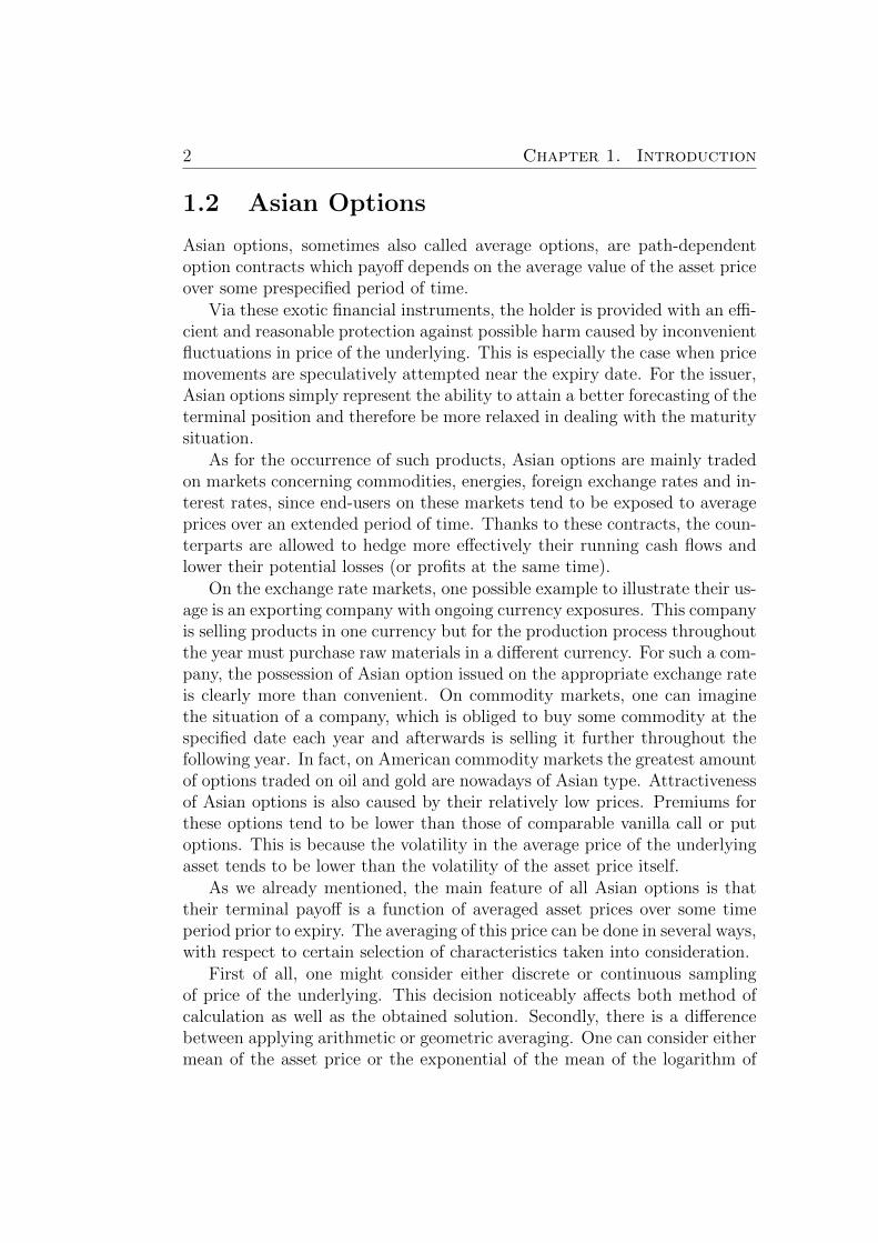
the asset price. In addition, one can decide about the period over whichthe average price is calculated. The period does not have to coincide withthe life time of the option. Finally, there is the question about weighted orunweighted average, since recent prices for instance might be for pricing theoption in some sense much more important (see Appendix for more details).
Figure 1.1: Comparison of continuous arithmetic and geometric averagingillustrated on historical prices of crude oil (inflation adjusted). Source ofdata: www.inflationdata.com.
For each different choice of these previously mentioned characteristics,the resulting solution might clearly differ. Because there is no way how toobjectively decide, which selection is more and which is less accurate, allpossible combinations have been already analyzed and have led to varioustechniques of pricing Asian options.
In fact, there are even more features, according to which Asian options canbe distinguished. The basic grouping is naturally into call options and putoptions. Another classification is into European type options and Americantype options. This means, that like in case of vanilla options there existcontracts with and without early exercise opportunity. Other specific featureis the way in which the average is incorporated into the payoff function. If wedenote the average value by A(T ), the following four basic payoff functionsare defined
(A(T )−K)+ average rate call(K − A(T ))+ average rate put
(S(T )− A(T ))+ average strike call(A(T )− S(T ))+ average strike put
4 Chapter 1. Introduction
The rate options are sometimes called price options, or fixed strike options;the strike options are also called floating strike options. If we compare thedepicted payoffs to those of plain vanilla options, for an average rate calloption the price term S(T ) is replaced by the average price term A(T ),whereas for the average strike option, the term A(T ) replaces the striketerm K.
1.3 Numerical Evaluation Techniques
Since exact analytic formulas for average rate and average strike options gen-erally do not exist, they are in point of fact much more difficult to evaluatethan common vanilla options. Furthermore, applying numerical methodsclassically used for pricing financial instruments often carries serious disad-vantages.
For example, in financial mathematics commonly used partial differentialequation (PDE) techniques are with regard to Asian options quite inaccurate,cf. [1]. Monte Carlo simulations with a specific variance reduction methodproposed by Kemna and Vorst [7] work well only considering European typeoptions and are still relatively slow. Conventional binomial lattice methodsare effectively unusable due to their huge requirements of computer memory.
As for American type Asian options, Hull and White [5] proposed a mod-ified binomial lattice method. Unfortunately, the convergence of this algo-rithm is questionable. Neave [9] used on a binomial lattice a frequency distri-bution approach. Here, calculations of order N4, where N is the number oftime steps in the lattice are required. Barraquand and Pudet [1] proposed anunconditionally convergent ”forward shooting grid” technique. In this thesis,we shall investigate modifications of finite difference (FD) methods.
As a matter of fact, the price of Asian option contract can be obtained asa numerical solution of a PDE problem, that has one dimension in time andtwo dimensions in space. We will refer to this equation as a two-dimensionalPDE. As we show later on, this PDE has convection-diffusion character, butwithout diffusion term in one of the spatial dimensions. This is very oftenthe reason of many numerical difficulties, especially occurance of spuriousoscillations. Moreover, for FD methods both the time and space complexitiesgrow exponentially in the number of state variables. Therefore one shouldtry to lower their number.
In most cases, the above mentioned two-dimensional PDE can be reducedinto a PDE with only one spatial dimension. There are at least three possibleways how to make this procedure. The first possible reduction, formulatedby Ingersoll [6] is applicable for case of average strike options. The same
Numerical Methods for Asian Options 5
property has the transformation of Wilmott, Dewinne and Howison [13].The last reduction method was proposed by Rogers and Shi [11] and can beapplied only for Asian options of European type.
In general, the one-dimensional PDE obtained from all previously intro-duced transformations is difficult to solve numerically. The reason is a noneor very small diffusion term in the derived PDE, which eventually causessolutions to oscillate. To eliminate these numerical instabilities, we shall for-mulate modifications to common methods to cope with this delicate problem.
One approach how to get rid of the oscillations caused by classically usedcentrally weighted schemes is to apply first-order upstream weighting for theconvective term (used in computational fluid dynamics). By this procedure,artificial diffusion is locally implemented into calculation and handles theoscillations. Unfortunately, one must point out that as a side-effect thisleads to results with excessive false diffusion. To additionally eliminate thisphenomenon, high order non-linear flux limiter can be applied. As we shalldemonstrate on the following pages, after such adjustment the resulting so-lutions are truly sufficiently accurate.
In Chapter 2 of this work, we are concerned with the derivation of PDEmodels to price Asian options. Chapter 3 is dedicated to depict problems,that might occur while numerically solving Asian option’s evaluation. With-out loss of relevance, this illustration is done on standard European vanillaoptions with a feature of small value of diffusion term, typical for averageoptions. In Chapter 4 we present numerical simulations and finally concludeour work in Chapter 5.
6 Chapter 1. Introduction
Chapter 2
PDE Models
2.1 Derivation of Two-dimensional Models
2.1.1 The Black-Scholes equation for path-dependentoptions
First we derive the general model for the valuation of all path-dependentoptions.
Consider the price function V (S(t), I(t), t). This function depends on thetime t, price process S(t) and the newly introduced path-dependent variable
I(t) =
∫ t
0
f(S(τ), τ)dτ, (2.1)
where the function f(.) is specific for each possible path-dependent optionconsidered. Since the variable I does not depend on the current asset priceS, the option price V is a function of three independent variables. The stockprice S(t) follows a classical geometrical Brownian motion (GBM)
dS = rSdt+ σSdB, (2.2)
where r represents the risk free interest rate, the variable σ is the volatilityand by dB we denote the standard Brownian motion. To apply Ito’s lemmaon V , we additionally need to know the stochastic differential equation (SDE)for variable I. This can be found very easily, since
I + dI = I(t+ dt) =
∫ t+dt
0
f(S(τ), τ)dτ =
∫ t
0
f(S(τ), τ)dτ + f(S(t), t)dt.
From this we clearly see, that
dI = f(S(t), t)dt. (2.3)
7
8 Chapter 2. PDE Models
Note that there is no stochastic component dB, only a drift component dt.Now we are allowed to apply the multidimensional Ito’s lemma on the
value function V (S(t), I(t), t) (see Appendix for the general form of thisformula). This procedure provides us with the expression
dV = σS∂V
∂SdB +
(1
2σ2S2∂
2V
∂S2+ rS
∂V
∂S+∂V
∂t+ f(S, t)
∂V
∂I
)dt. (2.4)
Let us now construct a risk-free portfolio Π by
Π = V −∆S,
dΠ = dV −∆dS, (2.5)
i.e., from a long position in option and short position in ∆-times underlyingasset. Substituting (2.2) and (2.4) into (2.5) yields
dΠ =
(σS
∂V
∂S−∆σS
)dB
+
(1
2σ2S2∂
2V
∂S2+ rS
∂V
∂S+∂V
∂t+ f(S, t)
∂V
∂I−∆rS
)dt
=
(σS
(∂V
∂S−∆
))dB
+
(1
2σ2S2∂
2V
∂S2+ rS
(∂V
∂S−∆
)+∂V
∂t+ f(S, t)
∂V
∂I
)dt.
To eliminate stochastic fluctuations from our portfolio, we should set ∆ =∂V/∂S. One is left with
dΠ =
(1
2σ2S2∂
2V
∂S2+∂V
∂t+ f(S, t)
∂V
∂I
)dt. (2.6)
If we adopt now the assumption of no arbitrage opportunities on the market,i.e., the change of our portfolio should coincide with the change of corre-sponding value of money deposited on the bank account earning risk-freeinterest rate, we obtain
dΠ = rΠdt = r(V −∆S)dt = r(V − ∂V
∂SS)dt. (2.7)
Putting together (2.6) and (2.7) leads to the general form of the Black-ScholesPDE for pricing path-dependent option contracts
∂V
∂t+
1
2σ2S2∂
2V
∂S2+ rS
∂V
∂S+ f(S, t)
∂V
∂I− rV = 0. (2.8)
Numerical Methods for Asian Options 9
2.1.2 The Black-Scholes equation for Asian options
As was already stated, various forms of the function f(.) specifies (2.8) forvaluing different path-dependent options. Considering the case of averagerate and average strike options, two basic possibilities arise. In the first one,we let the average value be defined as a running sum via the formula
I(t) =
∫ t
0
S(τ)dτ.
For variable I(t), first derivative with respect to time gives us the functionf(.) as
dI
dt= S(t) = f(S(t), t).
The Black-Scholes equation for Asian options in terms of variable I(t) takesthen the form
∂V
∂t+
1
2σ2S2∂
2V
∂S2+ rS
∂V
∂S+ S
∂V
∂I− rV = 0. (2.9)
Second common and equivalent concept for formulating average value is usu-ally denoted A(t) and defined by
A(t) =I(t)
t=
1
t
∫ t
0
S(τ)dτ.
Differentiation with respect to variable t gives function f(.) as expression
dA
dt=
1
tS(t)− 1
t2
∫ t
0
S(τ)dτ =1
t
(S(t)− 1
t
∫ t
0
S(τ)dτ
)=
=1
t
((S(t)− A(t)
)= f(S(t), t).
Therefore, in terms of A(t) the Black-Scholes PDE for Asian options takesthe form
∂V
∂t+
1
2σ2S2∂
2V
∂S2+ rS
∂V
∂S+
1
t(S − A)
∂V
∂A− rV = 0. (2.10)
As one can see, both depicted forms of the Black-Scholes PDE have a two-dimensional character. In other words, both PDEs include partial derivativesof the option price with respect to time and the two other state variables.However, neither equation (2.9) nor equation (2.10) has a diffusion term (sec-ond spatial partial derivative over respective variable) in the second spatialdimension. In fact, this feature causes many numerical instabilities whilenumerically solving with standard finite difference methods. We shall inves-tigate this in-depth in the following chapter.
10 Chapter 2. PDE Models
2.2 Reduction to One-dimensional Models
The more spatial dimensions the Black-Scholes equation has, the more com-plexity of FD methods is naturally incorporated into the process of pricingparticular options. In fact, both time and space complexities grow expo-nentially in the number of state variables. The two-dimensionality of thederived Black-Scholes PDEs for valuing Asian options is therefore a ratherunpleasant property.
Nevertheless, this undesirable feature can vanish, since in most cases cer-tain transformations are available which lead to reduction in spatial dimen-sions. This is not true only for American type average rate options whereeach time full two-dimensional PDE must be solved. We proceed here withillustrations of possible ways, how the reduction into one-dimensional PDEscan be done.
2.2.1 The Ingersoll method
As shown by Ingersoll [6], one possible reduction for average strike optionsmight be achieved by introducing the new variable R = S/I. Consider-ing the original pricing equation for function V (S(t), I(t), t) in form (2.9),appropriate boundary conditions are
V (0, I, t) = 0,
limS→∞
∂V
∂S(S, I, t) = 1,
limI→∞
V (S, I, t) = 0,
V (ST , IT , T ) =
(ST −
ITT
)+
.
Since in equation (2.9) appears only first partial derivative with respect tothe variable I, only one boundary condition in I direction is sufficient. Notethat all previously depicted boundary conditions together with equation (2.9)are lineary homogeneous in variables S and I. Therefore homogeneity holdsfor the option price V as well.
After the transformation R = S/I, the option price transforms intoV (S, I, t) = IG(R, t). Furthermore,
∂V/∂S = ∂G/∂R,
∂2V/∂S2 = (∂2G/∂R2)/I,
∂V/∂I = G−R(∂G/∂R),
∂V/∂t = I∂G/∂t.
Numerical Methods for Asian Options 11
In terms of the new value function G and new variable R, the pricing equationand boundary conditions become
1
2σ2R2∂
2G
∂R2+ (rR−R2)
∂G
∂R+ (R− r)G+
∂G
∂t= 0, (2.11)
G(0, t) = 0,
limR→∞
∂G
∂R(R, t) = 1,
G(RT , T ) = (RT − 1/T )+,
This approach can not be considered with average rate options, where the as-sumption of homogeneity in variables S and I is not fulfilled for the terminalcondition.
2.2.2 The Method of Wilmott, Dewinne and Howison
In contrast to the previously described method, Wilmott, Dewinne and How-ison [13] proposed a change of variables of inverse type:
Rt =ItSt
=1
St
∫ t
0
S(τ)dτ.
This causes the price function V to be transformed into a new function Hwith the relation V (S, I, t) = SH(R, t). The terminal payoff becomes
V (S, I, T ) =
(ST −
1
TIT
)+
= ST
(1− 1
TSTIT
)+
= ST
(1− 1
TRT
)+
= STH(RT , T ).
From
Rt+dt = Rt + dRt,
dSt = rStdt+ σStdBt,
follows the SDE
dRt = (1 + (σ2 − r)Rt)dt− σRtdBt.
In terms of H and R, equation (2.9) takes now the one-dimensional form
∂H
∂t+
1
2σ2R2∂
2H
∂R2+ (1− rR)
∂H
∂R= 0. (2.12)
12 Chapter 2. PDE Models
As for appropriate boundary conditions,
limR→∞
H(R, t) = 0,
∂H
∂t(0, t) +
∂H
∂R(0, t) = 0,
H(RT , T ) = (1−RT/T )+.
Similarly to the previous algorithm, this reduction works only in case ofaverage strike options.
2.2.3 The Method of Rogers and Shi
The approach formulated by Rogers and Shi [11] reduces the space dimensionsby introducing the new state variable
x =K −
∫ t0S(τ)µ(dτ)
St,
where µ is a probability measure with density ρ(t) on the interval (0, T ). Moreprecisely, ρ(t) = 1/T for average rate options and ρ(t) = 1/T − δ(T − t) foraverage strike options, where δ is a delta function.
The two-dimensional PDE for Asian options transforms in this case intoa one-dimensional equation of the form
∂W
∂t+
1
2σ2x2
∂2W
∂x2− (ρ(t) + rx)
∂W
∂x= 0. (2.13)
The terminal conditions are
w(x, T ) = x− (2.14)
for average rate call option and
w(x, T ) = (x+ 1)− (2.15)
for average strike put option, where (q)− = max(−q, 0).In the case where µ is uniform on [0, T ], the price of Asian option with
initial price S0, maturity T and fixed strike K is S0W (K/S0, 0). For anoption with floating strike but all other parameters the same is the priceequal to S0W (0, 0).
Let us remark, that on one hand the Rogers and Shi framework holds forboth average rate and average strike options. But on the other hand, it isnot applicable for Asian options of American type.
Chapter 3
Numerical Discretization
In this chapter we will focus on some basic ways in which discretization ofconsidered option models can be done. We will try to illustrate, what arethe possible problems and complications which might occur while applyingclassical discretization techniques and what could one eventually do to getrid of them. Our goal is therefore to analyze the classical way of treatmentand subsequently try to do effective adjustments so that one ends up withpractical method, which definitely provides fitting and accurate solutions.
Depiction of this matter is first done on classical European vanilla options.Afterwards, to make our point clear and understandable, transformation intoterms of Asian options is done.
3.1 Vanilla Options Discretization
As already stated, in case of Asian option contracts standard numerical dis-cretization leads often to oscillatory solutions. This feature also stands forclassical plain vanilla options which are convection-dominated (this propertyis discussed and explained later on). Instable spurious solutions are naturallyuntrustworthy (see Figure (3.1)). The numerical procedure must be thereforein all such cases clearly treated in quite a different way. The following textexplains, how to proceed.
European plain vanilla options can be priced by solving the well knownlinear parabolic Black-Scholes PDE
∂V
∂t+
1
2σ2S2∂
2V
∂S2+ rS
∂V
∂S− rV = 0, (3.1)
subject to appropriate boundary conditions and proper terminal condition.
13
14 Chapter 3. Numerical Discretization
Figure 3.1: Plain vanilla European Call price. Comparison of the Black-Scholes analytical solution and explicit numerical solution. (K = 15, T = 1,r = 0.15, σ = 0.01, ∆S = 0.1, ∆τ = 0.01)
For European call option, terminal and boundary conditions take theform
V (S(T ), T ) = (S(T )−K)+,
V (0, t) = 0,
V (S(t), t) ∼ S(t)−Ke−r(T−t) for S(t)→∞,respectively, whereas for European put option, the terminal condition is
V (S(T ), T ) = (K − S(T ))+
and the boundary conditions read
V (0, t) = Ke−r(T−t),
V (S(t), t) ∼ 0 for S(t)→∞.Since equation (3.1) is backward in time, one first needs to perform trans-
formation leading to a forward equation. This might be done by simply in-troducing the new reversed time variable, τ = T − t. Variable τ obviouslyruns from 0 to T and equation (3.1) after such substitution becomes
∂V
∂τ=
1
2σ2S2∂
2V
∂S2− (−rS)
∂V
∂S− rV. (3.2)
Numerical Methods for Asian Options 15
This equation is understood to be a convection-diffusion equation, where theterm
1
2σ2S2∂
2V
∂S2
is reffered to as a diffusion term and
(−rS)∂V
∂S
as a convective term. If in particular the ratio between these two terms,known as the Peclet number (convective coeff./diffusion coeff.), is very largeor in other words, diffusion term is very small comparing to convective term(σ � r), the equation is said to be convection-dominated. This is the caseof all PDEs for pricing Asian options. The numerical solution then behavesas if it was not parabolic equation but a hyperbolic one. Finding solutionsto such equation is therefore much difficult and demanding.
After applying on equation (3.2) one of possible finite volume discretiza-tion approaches, derived by Roache [10], we get the value at cell i at timestep n+ 1 represented as
V n+1i − V n
i
∆τ= θF n+1
i− 12
− θF n+1i+ 1
2
+ θfn+1i
+ (1− θ)F ni− 1
2− (1− θ)F n
i+ 12
+ (1− θ)fni .(3.3)
The lower index characterizes for variable its spatial position and upper indexrespective time layer. Variable θ stands for temporal weighting and holds,that 0 ≤ θ ≤ 1. For a fully-explicit method θ = 0, for a fully-implicit methodθ = 1 and to get the Crank-Nicolson method, one should let θ = 1
2. Terms
denoted by F are referred to as flux terms, those denoted by f as source/sinkterms. As for their detailed form,
F n+1i− 1
2
=1
∆Si
[(− 1
2σ2S2
i
)V n+1i − V n+1
i−1
∆Si− 12
+ (−rSi)V n+1i− 1
2
], (3.4)
F n+1i+ 1
2
=1
∆Si
[(− 1
2σ2S2
i
)V n+1i+1 − V n+1
i
∆Si+ 12
+ (−rSi)V n+1i+ 1
2
], (3.5)
fn+1i = (−r)V n+1
i , (3.6)
where
∆Si =Si+1 − Si−1
2, ∆Si+ 1
2= Si+1 − Si.
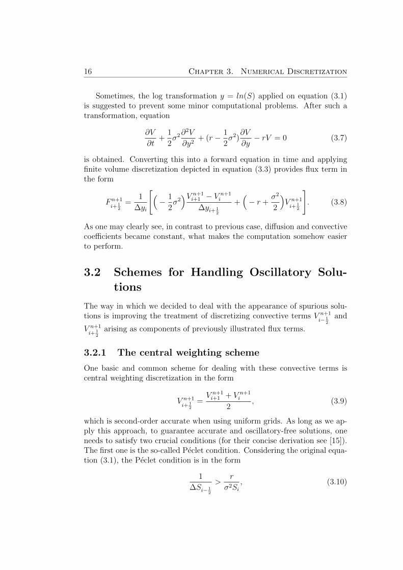
16 Chapter 3. Numerical Discretization
Sometimes, the log transformation y = ln(S) applied on equation (3.1)is suggested to prevent some minor computational problems. After such atransformation, equation
∂V
∂t+
1
2σ2∂
2V
∂y2+ (r − 1
2σ2)
∂V
∂y− rV = 0 (3.7)
is obtained. Converting this into a forward equation in time and applyingfinite volume discretization depicted in equation (3.3) provides flux term inthe form
F n+1i+ 1
2
=1
∆yi
[(− 1
2σ2)V n+1
i+1 − V n+1i
∆yi+ 12
+(− r +
σ2
2
)V n+1i+ 1
2
]. (3.8)
As one may clearly see, in contrast to previous case, diffusion and convectivecoefficients became constant, what makes the computation somehow easierto perform.
3.2 Schemes for Handling Oscillatory Solu-
tions
The way in which we decided to deal with the appearance of spurious solu-tions is improving the treatment of discretizing convective terms V n+1
i− 12
and
V n+1i+ 1
2
arising as components of previously illustrated flux terms.
3.2.1 The central weighting scheme
One basic and common scheme for dealing with these convective terms iscentral weighting discretization in the form
V n+1i+ 1
2
=V n+1i+1 + V n+1
i
2, (3.9)
which is second-order accurate when using uniform grids. As long as we ap-ply this approach, to guarantee accurate and oscillatory-free solutions, oneneeds to satisfy two crucial conditions (for their concise derivation see [15]).The first one is the so-called Peclet condition. Considering the original equa-tion (3.1), the Peclet condition is in the form
1
∆Si− 12
>r
σ2Si, (3.10)
Numerical Methods for Asian Options 17
for the log-transformed equation (3.7) in form
1
∆yi− 12
>|r − σ2
2|
σ2. (3.11)
Let us point out one problem, handled by the log transformation, which issatisfying the Peclet condition if S → 0. Considering (3.10), for S0 = 0 theimplied condition σ2
r> 1 must be fulfilled which may not be true. In the
latter case, none such a strict relation must be guaranteed.The second additional condition that must be taken into consideration
during the discretizing procedure takes the form
1
(1− θ)∆τ>σ2S2
i
2
(1
∆Si− 12∆Si
+1
∆Si+ 12∆Si
)+ r (3.12)
and1
(1− θ)∆τ>σ2
2
(1
∆yi− 12∆yi
+1
∆yi+ 12∆yi
)+ r (3.13)
for cases (3.1) and (3.7) respectively.Notice that if r is significantly large compared to σ (considered equation
is convection-dominated), to meet both additional and Peclet conditions onemust use a very fine grid spacing. To avoid this limiting and sometimesextremely demanding requirement, one may try to synthetically affect theconvection-diffusion ratio by numerically enlarging true diffusion of the modelby artificial diffusion. One possible implementation of this approach is byintroducing a first-order upstream weighting scheme, that is often used incomputational fluid dynamics.
3.2.2 The first-order upstream weighting scheme
This weighting method is first-order accurate on a uniform lattice. Its generalform is
V n+1i+ 1
2
=
{V n+1i if − rSi ≥ 0,V n+1i+1 otherwise.
Since we consider the Black-Scholes equation (3.1), the relation rSi ≥ 0holds. Therefore V n+1
i+ 12
= V n+1up = V n+1
i+1 .
18 Chapter 3. Numerical Discretization
Because evident one-sided differencing is applied through this scheme,requested synthetic diffusion is truly incorporated into the computationalprocess and the resulting solutions are after fulfilling only one condition
1
(1− θ)∆τ>σ2S2
i
2
(1
∆Si− 12∆Si
+1
∆Si+ 12∆Si
)+rSi∆Si
+ r, (3.14)
no longer unstable in terms of producing spurious oscillations. However, themethod still has some disadvantages. Among others, the main inconvenienceis certainly the fact, that artificial diffusion supplemented into numericalcalculation causes too diffused and hence inaccurate solutions. For the sakeof reliable outcomes, presence of this excessive diffusion must be furtheradjusted. We shall focus on this issue in the following subsection.
3.2.3 The van Leer flux limiter
In order to obtain reasonably accurate solutions without the threat of dealingwith both spurious oscillations and excessive diffusion, one has the possibilityto introduce the van Leer flux limiter. The aim of this approach is to augmenttrue diffusion of the model by additional numerical diffusion only if necessaryto prevent instabilities. The general formula for this method is
V n+1i+ 1
2
= V n+1up +
φ(qn+1i+ 1
2
)
2(V n+1
down − Vn+1up ), (3.15)
where the limiter function φ(.) is defined as
φ(q) =|q|+ q
1 + |q|(3.16)
and the variable q is defined as
qn+1i+ 1
2
=V n+1up − V n+1
2up
S2up − Sup
/V n+1down − V n+1
up
Sup − Sdown. (3.17)
The crucial feature of this scheme is the fact, that artificial diffusion is addedinto calculation only at specific grid points. In particular, at points wherethe gradient is steep, which as a result handles the former problem of diffusedsolutions. Consequently, the method has second-order accuracy on regionswhich are not affected by synthetic diffusion.
Numerical Methods for Asian Options 19
The guarantee of providing oscillation-free solutions is assured by scheme’stotal variation dimishing (TVD) property. TVD means that for the totalvariation of the solution, defined as
TV (V n+1) =∑i
|V n+1i+1 − V n+1
i |,
the following relation holds
TV (V n+1) ≤ TV (V n).
This outlined inequality clearly doesn’t allow any instabilities contained insolution, since any undesirable oscillations would naturally cause total vari-ation to increase and so to violate this relation.
3.3 Asian Options Discretization
Although in the previous text we were concerned with plain European vanillaoptions and their numerical treatment, now our goal is to put illustrated dis-cretization ideas into terms of Asian options. The already depicted gradualimprovement of handling problems, which may occur while numerically pric-ing special case of vanilla options, can be relatively easily transformed andapplied on Asian option contracts. This section is dedicated exactly to thismatter.
To recall, Asian options can be priced by solving two-dimensional PDE,either in form (2.9) or in form (2.10). As we already illustrated, there arecertain ways how the two-dimensionality can be eliminated and so one justneeds to deal with one-dimensional PDE which may not be that demanding.Discretization can be afterwards applied on an only one-dimensional PDEwhich is very favourable. Let us depict discretization treatment of two pre-sented PDEs, which is done analogically to the case of plain vanilla options.
If we consider the reduction proposed by Ingersoll, one deals with the PDE
1
2σ2R2∂
2G
∂R2+ (rR−R2)
∂G
∂R+ (R− r)G+
∂G
∂t= 0.
After the transformation into a forward equation, done by introducing thereversed time variable τ = T − t, one obtains the PDE
∂G
∂τ=
1
2σ2R2∂
2G
∂R2− (−rR +R2)
∂G
∂R+ (R− r)G. (3.18)
20 Chapter 3. Numerical Discretization
Now, if we apply the discretization scheme (3.3), the flux terms take the form
F n+1i− 1
2
=1
∆Ri
[(− 1
2σ2R2
i
)Gn+1i −Gn+1
i−1
∆Ri− 12
+ (−rRi +R2i )G
n+1i− 1
2
], (3.19)
F n+1i+ 1
2
=1
∆Ri
[(− 1
2σ2R2
i
)Gn+1i+1 −Gn+1
i
∆Ri+ 12
+ (−rRi +R2i )G
n+1i+ 1
2
](3.20)
and the sink term takes the form
fn+1i = (Ri − r)Gn+1
i . (3.21)
In case of considering the one-dimensional PDE
∂H
∂t+
1
2σ2R2∂
2H
∂R2+ (1− rR)
∂H
∂R= 0
proposed by Wilmott, Dewinne and Howison, transformation to forwardequation leads to PDE
∂H
∂τ=
1
2σ2R2∂
2H
∂R2− (rR− 1)
∂H
∂R.
Discretization scheme (3.3) may be then applied which provides flux termsin the form
F n+1i− 1
2
=1
∆Ri
[(− 1
2σ2R2
i
)Hn+1i −Hn+1
i−1
∆Ri− 12
+ (rRi − 1)Hn+1i− 1
2
], (3.22)
F n+1i+ 1
2
=1
∆Ri
[(− 1
2σ2R2
i
)Hn+1i+1 −Hn+1
i
∆Ri+ 12
+ (rRi − 1)Hn+1i+ 1
2
](3.23)
The sink term vanishes since considered PDE includes only partial derivativesof H.
For both methods, convective terms Gn+1i− 1
2
and Gn+1i+ 1
2
(alternatively Hn+1i− 1
2
and Hn+1i+ 1
2
) shall be treated just like we illustrated in section 3.2.
Chapter 4
Stable Numerical Valuation ofOptions
This chapter of the thesis is dedicated to practical results, which we ob-tained by gradually applying all previously mentioned theoretical methodsand knowledge. To perform numerical calculations, we decided to use themathematical software MATLAB. Two examples of the respective algorithmscreated in order to price the options can be found in Appendix.
4.1 Valuation of Vanilla Options
As already stated, problems which occur while pricing Asian options mightalso arise while pricing plain vanilla options. This is the case especially if thepricing PDE is convection-dominated. On the following pages, we concernwith exactly this situation. We shall try to numerically evaluate the plainvanilla call option, while intentionally considering small volatility and largeinterest rate.
First of all, we try to calculate the price of this option using usual conceptof central weighting scheme. After substitution done into flux terms (3.4)and (3.5) with respect to formula (3.9), substituting flux terms and sinkterms into scheme (3.3) and putting together all coefficients standing nextto the same grid points, one obtains an expression of the type
αn+1i V n+1
i−1 + βn+1i V n+1
i + γn+1i V n+1
i+1 = αni Vni−1 + βni V
ni + γni V
ni+1, (4.1)
which is well known from the finite difference methods. In particular, for
21
22 Chapter 4. Stable Numerical Valuation of Options
After setting appropriate boundary conditions and terminal condition and af-ter decision about temporal weighting (0 ≤ θ ≤ 1), finally the equation (4.1)can be written in the MATLAB code and the premium of the considered calloption can be calculated.
Figure 4.1: European Call price. Comparison of the Black-Scholes analyticalsolution and numerical solution, considering the central weighting scheme.(K = 15, T = 1, r = 0.15, σ = 0.01, ∆S = 0.1, ∆τ = 0.01, θ = 0)
Let us note once again that the ’convection-dominated’ feature typicalfor PDE models of Asian options is guaranteed by considering unrealisticvalues of the risk free interest rate and volatility, in particular r = 0.15 andσ = 0.01. As for other parameters, the strike price K = 15 and the timeto maturity T = 1. We perform the computation while using uniform gridspacing ∆S = 0.1, ∆τ = 0.01.
Numerical Methods for Asian Options 23
Figure 4.2: European Call price. Comparison of the Black-Scholes analyticalsolution and numerical solution, considering the central weighting scheme.(K = 15, T = 1, r = 0.15, σ = 0.01, ∆S = 0.1, ∆τ = 0.01, θ = 1)
Figure 4.3: European Call price. Comparison of the Black-Scholes analyticalsolution and numerical solution, considering the central weighting scheme.(K = 15, T = 1, r = 0.15, σ = 0.01, ∆S = 0.1, ∆τ = 0.01, θ = 1
2)
24 Chapter 4. Stable Numerical Valuation of Options
Illustrated results prove that the Crank-Nicolson temporal weighting pro-vides us with the most precise results in terms of general accuracy. However,as one may clearly see, while using the central weighting scheme and applyingexplicit discretization method (Figure (4.1)), the algorithm leads to apparentoscillatory results as predicted. As a matter of fact, in this particular casethe oscillations are caused by violation of the Peclet condition, which mayvery easily happen if solving Asian option PDEs. This is definitely not quitedesirable and neither considering implicit approach depicted on Figure (4.2)nor Crank-Nicolson approach shown on Figure (4.3) helps to improve han-dling the oscillations. Therefore, in order to obtain non-oscillatory outcomes,instead of the central weighting approach one needs to apply some other moresuitable method.
To move on with this matter and so to get rid of the unpleasent occu-rance of spurious oscillations, consider now the first-order upstream weightingscheme. If one derives the equation of the form (4.1) for this particular case,the coefficients read
To recall, this approach is based on the fact, that true diffusion of themodel is enlarged with some intended artificial diffusion. As a result, thediscretized PDE locally behaves as non-convection-dominated and so the fea-ture of providing oscillatory solution positively disappears. Values depictedon the Figure (4.4) proves our point. On this figure, plotted against theanalytical Black-Scholes solution, you may see results we obtained by calcu-lating price of the plain vanilla European call option considering upstreamweighting. Outcomes from all three basic temporal weighting approaches areillustrated.
On the one hand, oscillations truly disappeared from the obtained solu-tion. On the other hand, as suspected, the artificial diffusion incorporatedinto computational process seriously harmed the solution and caused it tobecome too diffuse. Unfortunately, such results are therefore absolutely notreliable and the upstream weighting scheme can not be accepted to be theproper method for solving such PDEs.
Numerical Methods for Asian Options 25
Figure 4.4: European Call price. Comparison of the Black-Scholes analyticalsolution and numerical solutions, considering the first-order upstream weight-ing scheme. (K = 15, T = 1, r = 0.15, σ = 0.01, ∆S = 0.1, ∆τ = 0.01)
Although supplementing the artificial diffusion into the model seems tobe right for handling problems with the instabilities, it must be treated differ-ently and more cautiously than by the first-order upstream weighting schemeso that the solution persists to be accurate. Let us therefore introduce thevan Leer flux limiter techniques into our calculations.
As derived and explained previously in theoretical part of this text, con-sidering flux limiter is expected to add the numerical diffusion only if neces-sary to prevent oscillations. The coefficients of equation (4.1) takes now theform
αn+1i = θ∆τ(−1
2σ2i2 + riφn+),
βn+1i = 1− θ∆τ(−σ2i2 − ri(1− φn+ − φn−)− r),
γn+1i = θ∆τ(−1
2σ2i2 − ri(1− φn−)),
αni = −(1− θ)∆τ(−1
2σ2i2 + riφn+),
βni = 1 + (1− θ)∆τ(−σ2i2 − ri(1− φn+ − φn−)− r),
γni = −(1− θ)∆τ(−1
2σ2i2 − ri(1− φn−)).
26 Chapter 4. Stable Numerical Valuation of Options
The variables φn+ and φn− represent the values of the limiter functions
φn+ =φ(qn
i+ 12
)
2, φn− =
φ(qni− 1
2
)
2
explained in detail in section 3.2.3. To simplify the computation, we decidedto substitute values φn+1
+ and φn+1− (originally appearing in the flux terms
F n+1i− 1
2
and F n+1i+ 1
2
) with values calculated at the previous time layer. Following
results show, that this simplification does not significantly affect accuracy ofthis method.
Figure 4.5: European Call price. Comparison of the Black-Scholes analy-tical solution and numerical solution, considering the van Leer flux limiterscheme. (K = 15, T = 1, r = 0.15, σ = 0.01, ∆S = 0.1, ∆τ = 0.01, θ = 0)
Figure (4.5) and Figure (4.6) illustrate, that although we incorporatedthe van Leer flux limiter, while using uniform grid spacing ∆S = 0.1 and∆τ = 0.01, the explicit and implicit method provide results that are still dif-fused and do not fit properly the call premiums given by the Black-Scholesanalytical solution (our benchmark). However, reasonably accurate resultsmight be calculated by these approaches while using finer grid spacing, e.g.considering time spacing ∆τ = 0.001, but after such modification the compu-tation becomes naturally much more time-demanding. This is true mainly incase of the implicit method. Therefore, one shall focus on the Crank-Nicolsonform of the van Leer flux limiter scheme.
Numerical Methods for Asian Options 27
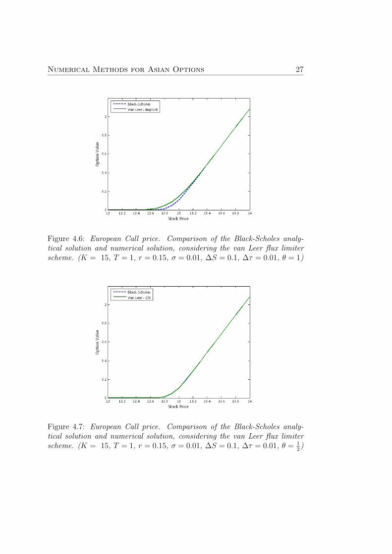
Figure 4.6: European Call price. Comparison of the Black-Scholes analy-tical solution and numerical solution, considering the van Leer flux limiterscheme. (K = 15, T = 1, r = 0.15, σ = 0.01, ∆S = 0.1, ∆τ = 0.01, θ = 1)
Figure 4.7: European Call price. Comparison of the Black-Scholes analy-tical solution and numerical solution, considering the van Leer flux limiterscheme. (K = 15, T = 1, r = 0.15, σ = 0.01, ∆S = 0.1, ∆τ = 0.01, θ = 1
2)
28 Chapter 4. Stable Numerical Valuation of Options
Judging from the Figure (4.7), the van Leer flux limiter technique jointlywith the Crank-Nicolson temporal weighting approach is truly the answer tothe established problems. As we declared in the theoretical part, this methodreally effectively handles instabilities of the resulting solution while addingjust appropriate measure of the artificial diffusion so that the outcome isaccurate and not over-diffused. If considering grid spacing ∆S = 0.1 and∆τ = 0.01, as depicted on Figure (4.7), prices of the call option given bythe Black-Scholes analytical formula and those provided by the algorithmbased on van Leer flux limiting are hardly distinguishable. As illustratedon Figure (4.8), the difference between these two premium curves is clearlyminimal and the obtained solution can be undoubtedly accepted as highlyaccurate.
Figure 4.8: European Call price. Difference between Black-Scholes analyticalsolution and numerical solution, considering the CN van Leer flux limiterscheme. (K = 15, T = 1, r = 0.15, σ = 0.01, ∆S = 0.1, ∆τ = 0.01, θ = 1
2)
Numerical Methods for Asian Options 29
4.2 Valuation of Asian Options
To properly verify the statement, that the van Leer flux limiting truly pro-vides us with highly accurate premiums while numerically pricing Asian op-tions, it is certainly reasonable to present some practical results.
Table 4.1: Comparison of the European Floating Strike Call premiums cal-culated while using the van Leer flux limiting (C-N temporal weighting) andpremiums calculated by Hansen & Jørgensen.
In order to do so, we decided to consider the transformed PDE (2.12), pro-posed by Wilmott, Dewinne and Howison, which as far as we are concernedhas not been studied yet in terms of the van Leer flux limiting. Based on
30 Chapter 4. Stable Numerical Valuation of Options
this PDE, we have created the MATLAB algorithm which numerically solvesthis equation (the code can be found in Appendix). We employed the Crank-Nicolson temporal weighting method. The representative European FloatingStrike Call premiums calculated with this algorithm are illustrated in Table4.1 and are compared to premiums calculated by Hansen & Jørgensen [4](our benchmark).
To briefly comment on the obtained values, as declared, the van Leer fluxlimiting truly appears to be efficient and very convenient approach while nu-merically pricing the Asian options. All the premiums in Table 4.1 providedby our algorithm differ from the benchmark premiums in less than 0.02. Inorder to reach such a high accuracy of results for various values of parameterT and still persist low execution time (we point out, that each illustratedprice in Table 4.1 was calculated within 20 seconds.), it was crucial to deter-mine the appropriate values for grid spacing. Hence, we present here to thereader three basic commands, that led to premiums in Table 4.1.
Let us also shortly comment on the issue of various flux limiters. Orig-inally, after calculating the Asian option premiums with the van Leer fluxlimiter, we wanted to compare these to premiums calculated with some otherknown limiters. However, after proving such a high accuracy of the van Leerapproach, this task seemed to us quite unreasonable.
In conclusion, at this point we are certainly allowed to state, that numer-ically solving convection-dominated PDEs such as the one for pricing vanillaoptions considered in previous section or those discribing prices of the Asianoptions by introducing the van Leer flux limiter can be understood to be theright choice, since the computation is not significantly time-demanding andprovided results are proven to be highly accurate.
Chapter 5
Conclusion
Dealing wide range of financial derivatives is nowadays part of everyday rou-tine on the markets all around the developed world. The valuation of allsuch liquid products is therefore expected to be clear, transparent, fast andmost of all, accurate. This master’s thesis was dedicated to fair and precisepricing of Asian option contracts, especially to the matter of handling theinstabilities which frequently occur while numerically valuing these optionsvia solution of the respective PDEs.
In Chapter 1, we introduced the reader into the concept of the Asian typeoptions, mentioning huge variety of their specific properties and unique fea-tures. We pointed out, that although original PDEs for their evaluation aretwo-dimensional in space, various reductions into one-dimensional PDEs areavailable. Since this procedure allows potential pricing algorithm to becomemuch less time-demanding, such a simplification is considered to be greatlyconvenient. At the end of this part, we went very briefly through a coupleof ways and methods, how numerical pricing of option contracts might beperformed.
Next chapter was dedicated to detailed derivation of PDE models associ-ated to these derivatives. Starting from the classical geometrical Brownianmotion, we introduced new path-dependent variable and applied the mul-tidimensional Ito’s lemma. After constructing the risk-free portfolio andadopting the no arbitrage assumption, we ended up with the general PDEfor pricing path-dependent options. Its specific form for the case of Asianoptions was derived as a following step. The second part of Chapter 2 wasthen concerned with concise depiction of three possible methods, in whichreduction of the PDE from two into one spatial dimension can be done.
The crucial property of being ’convection-dominated’, typical for PDEmodels of Asian options, was explained in Chapter 3. Without loss of rel-evance, depiction of this matter was done on the well known Black-Scholes
31
32 Chapter 5. Conclusion
PDE for pricing plain vanilla options. Problems, arising from this unpleasantfeature were subsequently introduced. The finite volume discretization ap-proach was illustrated together with the special form of its flux terms and sinkterms and on its basis appropriate methods for dealing with instabilities ofprovided numerical solution were shown. In particular, the central weightingscheme was presented, which leads to accurate solution only if two relativelystrict conditions are fulfilled. Therefore, the first-order upstream weight-ing scheme was introduced and both advantages and disadvantages of thisappproach were discussed. Afterwards the van Leer flux limiter technique,which might be seen as the efficient adjustment to the previous method, wasdepicted. Its TVD property which implies providing reasonably accuratenumerical solutions was theoreticaly demonstrated.
Finally, Chapter 4 consisted of practical results we obtained by creatingseveral MATLAB algorithms. In its first part, we analysed valuation of spe-cially designed plain vanilla options. As expected, under certain assumptionsand while using fixed uniform grid spacing in both time and space, the cen-tral weighting scheme classicaly used in discretization analysis did not pro-vide sufficient results. Visible oscillations occuring while using all three basictemporal weighting schemes were illustrated. So the upstream weightingscheme was analysed. It was proved by the outcomes, that this method trulyeliminates any oscillations from the obtained solution. However, while intro-ducing the artificial diffusion into the computation, this scheme affected thesolution to become over-diffused. This newly arising problem was effectivelymanaged later on by incorporationg the van Leer flux limiter. Through thismethod the artificial diffusion was added into the computation just appro-priately. The van Leer flux limiter scheme provided us with highly accurateresults, while in particular the calculated vanilla premiums differed from theBlack-Scholes analytical benchmark in less than 0.002. The second part ofthis chapter was then eventually dedicated to illustration and verification ofefficiency of the analysed approach in terms of the Asian options. Based onthe obtained results we were allowed to state, that the van Leer flux limit-ing can be without dispute accepted as convenient method for pricing theseexotic derivatives.
To sum up, the thesis illustrated the concept of the spurious oscillationsoccuring while pricing convection-dominated PDEs such as those associatedwith Asian option models and practically proven efficiency and applicabilityof the van Leer flux limiter approach, through which these problems mightby handled.
Notation
PDE Partial differential equation.
SDE Stochastic differential equation.
t Time.
T Expiration time.
K Strike price of an option.
S, S(t) Price of the underlying asset at time t.
I, I(t), A,A(t) Average price of the underlying asset at time t.
V, V (S, I, t) Price of the option at time t, asset’s price Sand asset’s average price I.
Π Risk-free portfolio.
(q)+ max(q, 0).
(q)− max(−q, 0).
r Risk-free interest rate.
σ Constant volatility.
τ Reversed time variable (τ = T − t).
θ Temporal weighting parameter (0 ≤ θ ≤ 1).
φ(.) Limiter function.
∆S Spacial step.
∆τ Time step.
Fni Flux term at time level n and spatial level i.
fni Source/sink term at time level n and spatial level i.
33
34
Bibliography
[1] J. Barraquand and T. Pudet (1996)Pricing of American Path-Dependent Contingent Claims. MathematicalFinance, 6, 17 – 51.
[2] T. Bokes and D. Sevcovic (2009)Early Exercise Boundary for American Type of Floating Strike AsianOption and Its Numerical Approximation. Quantitative Finance Papers0912.1321, arXiv.org.
[3] P. Brandimarte (2006)Numerical Methods in Finance and Economics : A MATLAB-BasedIntroduction. Second edition. John Wiley & Sons, Inc., Hoboken, NewJersey.
[4] A.T. Hansen and P.L. Jørgensen (1997)Analytical Valuation of American-Style Asian Options. SSRN eLibrary.
[5] J. Hull and A. White (1993)Efficient Procedures for Valuing European and American Path-dependentOptions. The Journal of Derivatives, 1, 21 – 31.
[6] J.E. Ingersoll, Jr. (1987)Theory of Financial Decision Making. Rowman & Littlefield Publishers,Inc., New Jersey.
[7] A. Kemma and A. Vorst (1990)A Pricing Method for Options Based on Average Asset Values. Journalof Banking and Finance, 14, 113 – 129.
[8] T.R. Klassen (2001)Simple, Fast, and Flexible Pricing of Asian Options. Journal of Compu-tational Finance, 4, 89 – 124.
35
[9] E. Neave (1994)A Frequency Distribution Method for Valuing Average Options. Workingpaper, School of Business, Queen’s University.
[10] P. Roache (1972)Computational Fluid Dynamics. Hermosa, Albuquerque, New Mexico.
[11] L. Rogers and Z. Shi (1995)The Value of an Asian Option. Journal of Applied Probability, 32 (4),1077 – 1088.
[13] P. Wilmott, J. Dewinne and J. Howison (1993)Option Pricing: Mathematical Models and Computation. Oxford Finan-cial Press, Oxford.
[14] P. Wilmott, J. Howison and J. Dewinne (1995)The Mathematics of Financial Derivatives. Cambridge.
[15] R. Zvan, P.A. Forsyth and K. Vetzal (1998)Robust Numerical Methods for PDE Models of Asian Options. Journalof Computational Finance, 1, 39 – 78.
36
Appendix
1. Different Methods of AveragingIn case of continuous sampling, one deals with a price process St. If this
process St is observed at discrete time moments ti, say equidistantly withthe time distance h := T/n, one is dealing with a times series St1 , St2 , . .. , Stn . If we denote the average value of asset price A(T ) and indices forarithmetical and geometrical average a and g respectively, in the discretecase
Aa(T ) =1
n
n∑i=1
Sti =1
Th
n∑i=1
Sti ,
Ag(T ) =
( n∏i=1
Sti
)1/n
= exp
(1
nlog
n∏i=1
Sti
)= exp
(1
n
n∑i=1
logSti
).
For continuously sampled price process, average value can be expressed asfollows:
Aa(T ) =1
T
∫ T
0
Stdt,
Ag(T ) = exp
(1
T
∫ T
0
logStdt
).
As for weighted averaging, one possible weightening method in case ofarithmetic average is by the formula
Awa (T ) =1∫ T
0a(t)dt
∫ T
0
a(T − t)Stdt,
where the kernel function a(.) ≥ 0,∫∞0a(t)dt < ∞ is usually defined as
a(t) = e−λt for some constant λ > 0.
37
2. Multidimensional Ito’s lemmaAssume, that the stochastic processes X
(i)t for i = 1, ..., n can be expressed
through the following stochastic differential equations:
dX(1)t
X(1)t
= µ(1)dt+ σ(1)dB(1)t ,
dX(2)t
X(2)t
= µ(2)dt+ σ(2)dB(2)t ,
...
dX(n)t
X(n)t
= µ(n)dt+ σ(n)dB(n)t ,
where d[B(i)t , B
(j)t ] = ρijdt.
Then, the general form of Ito’s lemma for any function f(X(1)t , ..., X
(n)t , t)
reads
df(X(1)t , ..., X
(n)t , t) =[(
∂
∂t+
n∑i=1
µ(i)X(i)t
∂
∂X(i)t
+1
2
n∑i,j=1
X(i)t X
(j)t σ(i)σ(j)ρij
∂2
∂X(i)t ∂X
(j)t
)f
]dt
+n∑i=1
∂f
∂X(i)t
σ(i)dB(i)t .
38
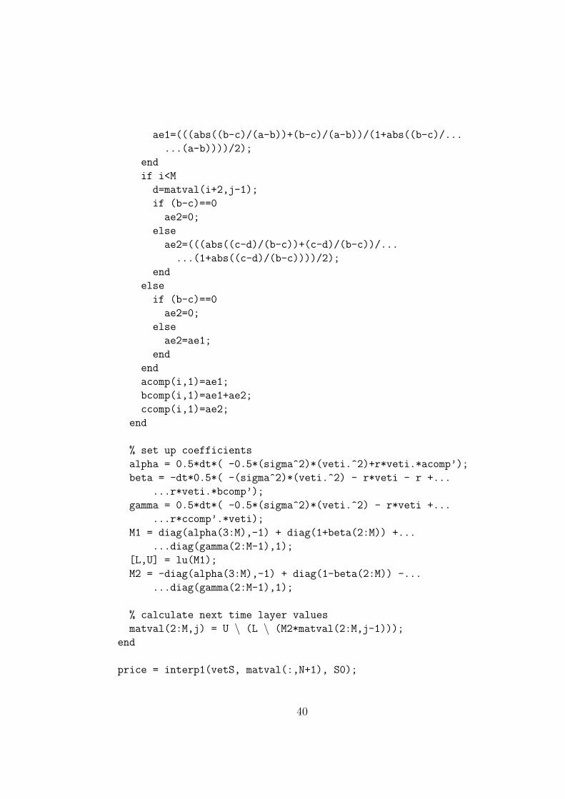
3. MATLAB code for European Vanilla Calloptions - the C-N van Leer flux limiter method


![Spatiotemporal dynamics of continuum neural fields...partial differential equation (PDE) models of diffusively coupled excitable systems [13, 14], neural field models can exhibit](https://static.documents.pub/doc/80x56/5f700c514eff5425e92b0db3/spatiotemporal-dynamics-of-continuum-neural-fields-partial-differential-equation.jpg)


