Stage long de recherche FIP M1 ´ Etude des collisions entre atomes froids de rubidium et un gaz chaud Study of collisions between cold rubidium atoms and a hot background gas Gabriel Dufour February 8 -July 12 2010 Supervisors: Kirk Madison James Booth Quantum Degenerate Gas Laboratory University of British Columbia Vancouver, Canada
Transcript
Stage long de rechercheFIP M1
Etude des collisions entre atomes froids derubidium et un gaz chaud
Study of collisions between cold rubidium atomsand a hot background gas
Gabriel Dufour
February 8 -July 12 2010
Supervisors:
Kirk MadisonJames Booth
Quantum Degenerate Gas LaboratoryUniversity of British Columbia
Vancouver, Canada
Abstract
Le systeme etudie consiste en un ensemble d’atomes de rubidium refroidisdans un piege magneto-optique puis transferes dans un piege magnetiquequadrupolaire. Nous avons cherche a caracteriser l’effet d’un gaz residuel(10−8 − 10−9 Torr) a temperature ambiante sur ce systeme. Une collisionavec un atome chaud peut causer la perte d’un atome piege, mais pourles grands parametres d’impact le transfert d’energie est insuffisant pourque l’atome sorte du piege. Ainsi, on observe a la fois une perte d’atomesdu piege et l’augmentation de l’energie moyenne des atomes restants. Nousavons mesure ce rechauffement experimentalement en sondant la distributiond’energie des atomes a l’aide d’ondes radio. De plus nous avons mis au pointune simulation directe du piege tenant compte du mouvement des atomeset des collisions avec le gaz chaud. Ces collisions sont regies par la sectionefficace differentielle calculee numeriquement a partir de premiers principes.La comparaison entre experience, simulation et des modeles simples doitconfirmer que les principaux mecanismes a l’œuvre sont bien compris etqu’ils peuvent etre mesures et predits.
We have studied an ensemble of rubidium atoms cooled in a magneto-optical trap and transferred into a magnetic quadrupole trap. The goal wasto characterize the effects of a room-temperature residual background gas(10−8− 10−9 Torr) on this system. A collision between a trapped atom anda background particle can cause the former to be lost from the trap, but forglancing collisions this is not always the case: the energy transferred to thetrapped atom might not be sufficient for it to leave the trap. Therefore, asatoms are lost from the trap, we also expect to see the average energy ofthe remaining atoms increase. This heating was experimentally measuredusing a radio-frequency field to probe the energy distribution in the trap.Moreover, a direct numerical simulation of the trap was designed. It takesinto account the classical motion of atoms inside the trap and collisions withbackground atoms. These collisions are governed by the differential cross-section, which was calculated numerically from first principles. Comparingexperiment, simulation and simple theoretical models should confirm thatthe mechanisms at work are well understood and that they can be measuredand predicted.
Before I start, I wish to thank Kirk Madison for welcoming me into his lab. Thanksto him this internship was an interesting, pleasant and inspiring experience.
I am very grateful to James Booth for his patience and good spirits whenintroducing me to the apparatus and guiding me through the experiments, as wellas for his valuable advice on theoretical questions.
It was a great privilege and pleasure to work with Charles Zhu. He has putan impressive amount of energy into this project. I wish him all the best for hisstudies in Toronto.
Thanks also to Dallas Clement, who is taking over this project with a lot ofenthusiasm and competence.
Janelle Van Dongen was a good fairy to all of us, always ready to help andalways successful in doing so.
Thank you to Will Gunton, Ben Deh, Mariusz Semczuk, Bruce Klappauf, Zhiy-ing Li and Ovidiu Toader for their competence, conversation and company.
I am indebted to David Fagnan for laying out the bases for this work.Enfin, je voudrais remercier ceux qui a l’Ecole Normale, ont rendu ce stage
possible, notamment Mascia Reato, Nicolas Mordant et Frederic Chevy.
Introduction
This report sums up the work I have been involved in during a 5 month stay in theQuantum Degenerate Gas laboratory (QDG) at the University of British Columbia(UBC) in Vancouver. This internship was supervised by Dr Kirk Madison fromUBC and Dr James Booth from the British Columbia Institute of Technology(BCIT).
The main subjects of interest in the QDG lab are
• the creation of cold polar molecules in an optical lattice,
• the characterization of loss and heating in pure-magnetic and magneto-optical traps.
I was involved in the latter project.
Interest in loss and heating processes in atom traps arose when contemplatingthe feasibility of a miniature atom trap. The lifetime of atoms in a trap is limitedby collisions with hot atoms from the residual background vapour. Such collisionsoften impart enough kinetic energy to the trapped atoms for them to escape thetrapping potential. Therefore a good vacuum (on the order of 10−8 Torr) is indis-pensable to trap atoms for more than a few seconds. However pumping systems
3
take up a lot of space, so a miniature trap might have to do without one. Theplan was to trap atoms in a sealed cell under high vacuum. But it appeared thatgases released from the cell walls prevented the formation of long-lived traps.
Nevertheless, this attempt drew attention to the fact that some backgroundgases affect atom traps more than others. Indeed, the loss rate from the trapdepends on the collisional cross-section between trapped atoms and backgroundatoms. Therefore trap loss is more than just a hindrance: it provides a tool toinvestigate cross-sections. Collisions range from glancing collisions with a largeimpact parameter to very energetic head-on collisions. Given a trap depth, onlysome of these collisions will contribute to loss. Measuring loss rates for varioustrap depths is therefore a way of characterizing this distribution of collisions. Thiswas done prior to my arrival by studying the evolution of trapped 87 rubidium inthe presence of a background vapour of 40 argon [8].
After having characterized losses from a magnetic trap, the team’s focus shiftedto heating. The glancing collisions mentioned above do not involve a large enoughenergy transfer to cause the loss of the trapped particle, but they do affect thatparticle’s energy. The overall effect of such collisions is an increase of the averageenergy per particle in the trap1.
Before we start, let me sum up the main goals that were set during his intern-ship:
• experimentally observe and quantify heating in a magnetic trap,
• predict and observe the dependence of heating with respects to trap depth,background pressure and the temperature of the trapped atoms
• and create an accurate direct numerical simulation of the system, compareits results with the experiment and use it to make predictions.
Although I have participated in the pursuit of all of these goals, the mainfocus of my work was the last objective: simulating the system to get a betterunderstanding of it.
1 Theoretical background
The object of this section is to provide a quick overview of the concepts I will bedealing with further on in this report. It is by no means exhaustive, please look-upthe references for more details.
1I might refer to this average energy per particle as a temperature in this report (E = kBT ,wth kB the Boltzmann constant). This should be seen as a convenient change of units ratherthan as a statement on the thermodynamics of the system. Indeed, our system is way out ofequilibrium and the strict definition of temperature does not apply.
4
1.1 Trapping neutral atoms
First of all, I will describe the principles behind the trapping of atoms using lightand/or magnetic fields.
1.1.1 Magnetic trap
In an atom, the nuclear and electronic spins (I and S) and the electronic orbitalangular momentum (L) all contribute to an atomic magnetic moment µ. Its am-plitude is described by the quantum number F . In a magnetic field, the projectionof this moment along the field takes quantized values gFµBmF , where gF is theLande g-factor 2, µB is the Bohr magneton and mF = −F,−F + 1, . . . , F . Theenergy of an atom in a magnetic field B is shifted by ∆E = −µ ·B. Thereforeatoms with the same F but different mF numbers will be degenerate in energy ifthere is no magnetic field and that degeneracy will be lifted in the presence of afield. This is referred to as Zeeman splitting.
The states for which µ and B are aligned will have a lower energy in higherfields (high-field-seeking states) whereas those for which µ and B are anti-alignedwill have a lower energy in smaller fields (low-field-seeking states). In free-space amagnetic field maximum cannot be achieved, but a local minimum can, and thisminimum will be seen as a potential well by low-field-seeking atoms.
It should be noted here that the direction of the field is not necessarily uniform.When an atom moves in an inhomogeneous field, its magnetic moment will followthe local magnetic field so long as the variations of the field are not too fast. Inthat case the motion is said to be adiabatic. However if the magnetic field changesquickly, the atom cannot follow and a trapped, anti-aligned state might suddenlyfind itself aligned and be lost from the trap (figure 1).
Figure 1: A case of Majorana spin-flip: the atom crosses the magnetic field zeroand goes from being anti-aligned (trapped) to aligned (lost).
2The Lande g-factor is a dimensionless proportionality constant that depends on I, L and S.
5
This type of diabatic process is called a Majorana spin-flip, it is liable to happenif the rate of change of the magnetic field (due to the atom’s motion) becomes ofthe same order as the frequency associated with the transition [11]:
v · ∇B
B∼ µ ·B
~, (1.1)
The simplest setup to create a magnetic field minimum consists of two coils inanti-helmholtz configuration. That is two coils aligned along the z-axis, separatedby a distance D and carrying a current I running in opposite directions. Thesetwo magnetic dipoles with opposite directions form a magnetic quadrupole, hencethe name quadrupole trap.
Figure 2: Shape of the potential seen by an atom in the xz-plane of a mag-netic quadrupole trap. The potential increases linearly with the coordinatec =
√x2 + y2 + (2z)2.
Near the centre of the trap, the magnetic field amplitude varies linearly withdistance from the minimum. The radial field gradient is half the axial gradient.The magnetic field goes to zero and changes sign in the centre (figure 2), whichraises the question of Majorana losses. If B = b′x, with x a position coordinate,the condition given in equation (1.1) becomes:
x2 ∼ ~µb′
(1.2)
This defines the surface through which an atom has to pass to undergo a spin-flip.The associated loss rate is:
ΓMajorana ∼ nx2v ∼ n~v2
µb′∼ n
~kBTmµb′
(1.3)
6
where n is the density, v is a typical speed and kBT is an energy scale for trappedatoms. In typical conditions for our experiment, this rate is on the order of 10−7
s−1 (versus 10−1 s−1 for collisional losses), so we will neglect Majorana losses.To the linear potential felt by low-field-seeking atoms because of their inter-
action with the magnetic field, one must add the gravitational potential (thoughit is relatively small in most cases). The trap depth is generally limited by theglass walls of the vacuum cell: atoms that reach the room-temperature walls areinstantly heated and lost from the trap.
1.1.2 The radio-frequency knife
The Zeeman splitting between different mF states is in the radio-frequency (RF)range. Therefore, an RF field can cause magnetic dipole transitions between thesestates [5]. But we have seen in the last paragraph that only certain mF statesare trappable (i.e. are low-field-seeking), so the RF can be used to eject atomsfrom the trap. Since the magnetic field amplitude is position dependent, so isthe energy splitting between different states. As a consequence the RF will onlybe resonant with a transition at a precise position, that is, at a given potentialenergy. The RF frequency ν defines a closed surface around the centre of the trap,and all particles that cross that shell are lost from the trap. Since only particleswith a total energy, potential and kinetic, larger than hν can reach that shell, andassuming that they do so in at most a few hundred microseconds, the RF can beused to empty out all atoms with energies hν or larger (figure 3). Its ability to“cut” energy distributions has earned this technique the name of “RF knife”. Ofcourse, the RF knife can also be used to set the trap depth.
1.1.3 Magneto-optical trap
The magnetic trap can only trap atoms that are already cold, therefore, it hasto be loaded from another type of trap that actively captures and cools atoms: amagneto-optical trap (MOT).
When photons scatter off an atom, they transfer some momentum to that atom,i.e. the atom experiences a force (called radiation pressure). A magneto-opticaltrap ingeniously uses that force to capture and trap atoms.
The scattering of photons off atoms can be seen as a process of absorption andre-emission. When the photon is absorbed, it transfers its momentum ~k to theatom. When the atom spontaneously re-emits, it recoils by −~k∗, where k∗ isthe wave-vector of the emitted photon, which is equal in amplitude to k but israndom in direction. If an atom scatters a great number of photons coming fromone direction, the absorptions will all push the atom in the same direction, butthe effect of the emissions will average out. Thus the atom experiences a net forcein the direction of k (figure 4).
The rate at which a two-level atom scatters photons is given by the lorentzian[7, 14]:
7
Figure 3: The RF knife transitions atoms of a given potential energy to an un-trappable state, causing them to be lost from the trap. We assume that all atomswith a total energy above hν have undergone a transition after a few hundredmilliseconds. The energy levels shown here correspond to an atom in the F = 1state (mF = −1, 0,+1).
Figure 4: The net force on an atom scattering photons is in the direction of theincoming light. Indeed the momenta transferred to the atom add up whereas therecoils due to spontaneous emission cancel out.
8
r =γ
2
s0
1 + s0 + (2δ/γ)2(1.4)
where γ is the spontaneous emission rate from the upper state and s0 = I/Isat isthe saturation parameter, ratio of the light intensity I and the saturation intensityIsat, which depends on the properties of the atom. The detuning δ = ω − ω0 isthe difference between the light’s angular frequency and the frequency associatedwith the energy gap in the two level atom.
Since each scattering event transfers a momentum ~k to the atom on average,the radiation pressure3 is given by:
F =γ
2
s0
1 + s0 + (2δ/γ)2~k (1.5)
At a given intensity, this force decreases when the absolute value of the detuningincreases.
A moving atom will see a Doppler-shifted light frequency: if the atom is trav-elling at v in the direction of the light’s propagation,
ω = ωl(1−v
c) (1.6)
Where ωl is the light’s frequency in the lab frame.Therefore the detuning is a function of the atom’s velocity: if δl = ωl − ω0,
δ = ωl(1−v
c)− ω0 = δl − kv (1.7)
An atom lit by a red-detuned laser4 will scatter more photons if it is travellingtowards the light source (v < 0) than if it is travelling away from it (v > 0).
Now if red-detuned light is shone on an atom from two opposite directions, theatom will experience two opposing forces, but the strongest of the two will alwaysoppose his velocity. Indeed, the resultant force is:
Fres =γ
2
(s0
1 + s0 + (2(δl − kv)/γ)2− s0
1 + s0 + (2(δl + kv)/γ)2
)~k (1.8)
Fres '8~k2s0δl/γ
(1 + s0 + (2δl/γ)2)2v (1.9)
Since δl is negative, this is a friction force. This effect is called Doppler cooling.If six red-detuned laser beams are shone in the ±x ,±y ,±z directions, atoms willbe slowed whatever the direction they are travelling in: we have a so called 3Doptical molasses.
Atoms that enter the molasses experience a force which depends on their veloc-ity but has no spatial dependence. When an atom’s velocity nears zero, the friction
3It is really a force.4A red-detuned laser has a frequency ωl < ω0 (δl < 0), a blue detuned laser has a frequency
ωl > ω0 (δl > 0).
9
force also goes to zero and the random recoils due to spontaneous emission causethe atom to undergo a random walk in momentum space, eventually leading it outof the molasses. This is a typical example of Brownian motion. A consequenceof this is the Doppler limit to cooling which is reached when the diffusion of themomentum prevents any further cooling5 [9, 14].
To introduce a spatial dependence to the radiation pressure, an inhomogeneousmagnetic field is applied. As we have seen in section 1.1.1, an atom’s energy levelsare slightly shifted in a magnetic field due to the Zeeman effect, and that shiftdepends on the quantum number mF and on the magnetic field amplitude. Theenergy difference between a | F,mF 〉 ground state and a | F ′,m′F ′〉 excited state istherefore a function of the local magnetic field, and so of the position. Actually,if the magnetic field is a quadrupolar field (as described in section 1.1.1), themagnetic field amplitude increases linearly with position6, and so does the Zeemansplitting.
To illustrate, let us consider the transition from a F = 0 ground state (mF = 0)to a F ′ = 1 excited state (m′F ′ = −1, 0,+1)7. Polarized light can be used to driveonly certain transitions. Left-circularly-polarized light (denoted σ−) only allowstransitions with m′F ′ = mF − 1 whereas right-circularly-polarized (σ+) light onlyallows m′F ′ = mF + 1 transitions. Suppose σ− light is shone from the side wherethe Zeeman shift brings the m′F ′ = −1 state closer to resonance (let this be theright-hand side, as in figure 5) and σ+ is shone from the opposite direction (theleft-hand side in figure 5). An atom on the right of the magnetic zero will morelikely undergo the near-resonant transition to m′F ′ = −1 and therefore absorb moreσ− photons and be pushed back to the centre of the trap. Conversely an atom inthe left-hand side region will absorb more σ+ photons that allow it to make thenear-resonant transition to m′F ′ = +1.
This clever combination of magnetic field and circularly-polarized light createsthe missing position-dependent force (figure 6): now the MOT can capture atomsfrom a vapour, cool them and trap them.
1.2 Collisions with the background gas
1.2.1 Classical collision kinematics
Consider two colliding particles of masses m1 and m2 and of velocities v1 and v2.They interact through a short-range potential V (r), where r = r1 − r2 is thevector that joins the two particles. The collision being a brief and violent event,we can suppose that these two particles are isolated (the effect of exterior forcesis negligible in such a short time).
5Another source of heating is the irregularity with which photons are absorbed, which leadsto “jiggling” of the atoms
6Near the centre of the trap.7This scheme also works in more complex cases.
10
Figure 5: The non-uniform magnetic field creates a position-dependent trappingforce by bringing atoms closer to resonance with the light that is pushing themtowards the centre of the trap.
Figure 6: Diagram of a magneto-optical trap showing the six contra-propagatingbeams and their polarizations, as well as the coil currents and magnetic field lines.
11
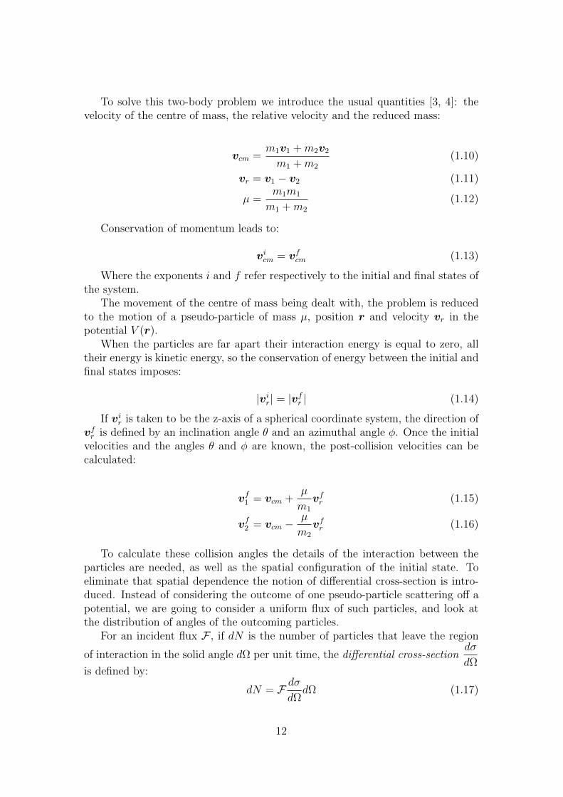
To solve this two-body problem we introduce the usual quantities [3, 4]: thevelocity of the centre of mass, the relative velocity and the reduced mass:
vcm =m1v1 +m2v2
m1 +m2
(1.10)
vr = v1 − v2 (1.11)
µ =m1m1
m1 +m2
(1.12)
Conservation of momentum leads to:
vicm = vfcm (1.13)
Where the exponents i and f refer respectively to the initial and final states ofthe system.
The movement of the centre of mass being dealt with, the problem is reducedto the motion of a pseudo-particle of mass µ, position r and velocity vr in thepotential V (r).
When the particles are far apart their interaction energy is equal to zero, alltheir energy is kinetic energy, so the conservation of energy between the initial andfinal states imposes:
|vir| = |vfr | (1.14)
If vir is taken to be the z-axis of a spherical coordinate system, the direction ofvfr is defined by an inclination angle θ and an azimuthal angle φ. Once the initialvelocities and the angles θ and φ are known, the post-collision velocities can becalculated:
vf1 = vcm +µ
m1
vfr (1.15)
vf2 = vcm −µ
m2
vfr (1.16)
To calculate these collision angles the details of the interaction between theparticles are needed, as well as the spatial configuration of the initial state. Toeliminate that spatial dependence the notion of differential cross-section is intro-duced. Instead of considering the outcome of one pseudo-particle scattering off apotential, we are going to consider a uniform flux of such particles, and look atthe distribution of angles of the outcoming particles.
For an incident flux F , if dN is the number of particles that leave the region
of interaction in the solid angle dΩ per unit time, the differential cross-sectiondσ
dΩis defined by:
dN = F dσdΩ
dΩ (1.17)
12
The total cross-section is defined as the integral of the differential cross-sectionover all solid angles:
σ =
∫dσ
dΩdΩ (1.18)
It has the units of an area: classically it can be seen as the effective surface thetarget particle presents to the incoming flux. Note that it generally is a functionof the relative speed vr.
1.2.2 Calculation of the differential cross-section
The differential cross-section can be obtained by using a simple quantum-mechanicalmodel.
As in the classical case, the quantum two-body problem can be reduced tosolving for a pseudo-particle of mass µ scattering off a potential V (r) [5, 4]. TheHamiltonian of the system is:
H =p2r
2µ+ V (r) (1.19)
The time independent solutions of Schrodinger’s equation verify:[− ~2
2µ∆ + V (r)
]ψ(r) = Eψ(r) (1.20)
Where E is the energy of the system.Suppose that V (r) tends to zero faster than 1/r as r goes to infinity, i.e. the
interaction takes place in a limited volume (this is verified by a typical Lennard-
Jones potential V (r) =C12
r12−C6
r6). In that case, the potential term can be neglected
at large r. Therefore the total energy of the system, E, is the incoming particle’sinitial kinetic energy and the wave function at large r is a solution of Schrodinger’sequation for a free particle.
Remember that our goal here is to obtain the probability distribution for theangles θ and φ given a uniform incident flux. This prompts us to write the wavefunction at large r as the sum of an incoming plane wave and a scattered sphericalwave, which are both solutions of the free-particle equation (figure 7):
ψ(r) ∼r→∞
N
(eikz + f(k, θ, φ)
eikr
r
)(1.21)
Where N is a normalization factor8 and k =
√2µE
~.
8We are leaving the problem of normalization aside, as the constant N will cancel out anyway.
13
Figure 7: The wave function is supposed to tend asymptotically to the sum of twosolutions of the free Schrodinger equation: an incoming plane wave and a scatteredspherical wave.
The probability current density associated to that wave function sheds light onthe reasons behind that choice. It is defined by [5, 4]
j(r) =~
2iµ(ψ(r)∗∇ψ(r)− ψ(r)∇ψ(r)∗) (1.22)
The current density associated with the plane wave is:
jin(r) = |N |2~kµ
= |N |2vr (1.23)
It has the form of a uniform flux of particles with speed vr.The current associated with the spherical wave is:
jout(r) = |N |2~kµ
|f(k, θ, φ)|2
r2(1.24)
The current through an element of surface r2dΩ is |N |2~kµ|f(k, θ, φ)|2dΩ. Thus
the fraction of incident flux which is deflected into the solid angle dΩ is |f(k, θ, φ)|2dΩ.By definition of the differential cross-section,
dσ
dΩ= |f(k, θ, φ)|2 (1.25)
At that point, let us make another hypothesis: V (r) = V (r) is a central poten-tial. Again, the Lennard-Jones potential satisfies that condition. Then the problemhas cylindrical symmetry around the z-axis (as defined in figure 7). Therefore, thewave function ψ(r) is independent of the azimuthal angle φ and it can be expandedin a Legendre series:
ψ(r, θ) =+∞∑l=0
Rl(r, θ)Pl(cos θ) (1.26)
14
where Pl is the lth Legendre polynomial. This is known as the partial wave ex-pansion [5, 4]. The lth partial wave has an angular momentum l. To satisfy theboundary condition given in equation (1.21), it can be shown that Rl must tendasymptotically to:
Rl(r, θ) ∼r→∞
1
kr(2l + 1)ileiδl sin(kr − lπ
2+ δl) (1.27)
Where δl is a real constant called the phase shift of the lth partial wave. Thescattering amplitude f(k, θ) can then be written:
f(k, θ) =1
k
+∞∑l=0
(2l + 1)il sin δlPl(cos θ) (1.28)
We can then go about solving Schrodinger’s equation to find the phase shifts δl.How this is done numerically has been detailed in [7] using a technique describedin [10].
1.3 Losses and heating
1.3.1 Trap loss
Consider the collisions of a trapped atom of initial velocity vt with backgroundatoms of initial velocity vb
9. The trapped atom sees a flux of such backgroundparticles equal to:
F(vb) = nbd(vb)(vb − vt) (1.29)
where nb is the background gas density (supposed to be constant in the cell) andd(vb) is the probability distribution function for the background particle’s velocity,i.e. the Maxwell-Boltzmann distribution at T = 300 K.
The fraction of that flux that will end up making an angle between θ and θ+dθwith the direction of the flux is:∫ 2π
0
(dσ
dΩsin θdθ
)dφ = 2π
∣∣∣f (k =µvr~, θ)∣∣∣2 sin θdθ (1.30)
Only some of these collision angles correspond to a final velocity for the trappedparticle that will make it leave the trap.
To simplify, let us suppose that the trapped particle is initially static, i.e.
vit = 0. In that case vir = vib, vcm =mb
mb +mt
vib and equation (1.16) becomes
vft =mb
mb +mt
(vir − vfr
)9I am keeping the same notations as in the previous section, except the index 1 is replaced
by b, for background particle, and the index 2 is replaced by t, for trapped particle. I amalso dropping the exponent i, all velocities referred to being initial velocities, unless otherwisespecified.
15
So the energy transferred by a collision of angle θ to the trapped atom is:
∆E =µ2
mt
vi2b (1− cos θ) (1.31)
If U is the trap depth, a collision will expel the atom out of the trap if [1, 2, 8]:
∆E > U (1.32)
or θ > θmin, (1.33)
where θmin = arccos
(1− Umt
µ2vi2b
)(1.34)
If we define the partial loss cross-section:
σU(vb) = 2π
∫ π
θmin
∣∣∣f (θ, kr =µvb~
)∣∣∣2 sin θdθ, (1.35)
the rate at which the trapped atom is being driven out of the trap by particlesof velocity vb is [8]:
F(vb)σU(vb) = nbd(vb)vbσU(vb) (1.36)
To obtain the total loss rate for a trapped atom, the previous expression mustbe integrated over the background velocities:
ΓU = nb
∫∫∫d(vb)vbσU(vb)dvb = nb〈σUvb〉 (1.37)
For simplicity, we will only write
Γ = nb〈σv〉 (1.38)
when this is not ambiguous. 〈σv〉 is known as the loss rate coefficient.
Figure 8: Theoretical loss rate coefficient 〈σUv〉 versus trap depth U for the collisionof 300 K rubidium atoms with static rubidium atoms.
16
1.3.2 Trap population
If several background gases are present, the loss rate is the sum of their contribu-tions.
Γ = nb1〈σv〉1 + ...+ nbi〈σv〉i (1.39)
In the magnetic trap nothing compensates for this loss and the number of atomexponentially decays:
NMT (t) = NMT (0)e−Γt (1.40)
In the MOT, however, the atoms are actively being captured at a rate R.Moreover the presence of excited state atoms with large cross-sections leads tolight-assisted collisions between trapped atoms [16]. The losses associated to thesecollisions are characterized by the constant β and are proportional to the overlapof the cloud with itself. The equation for the trap population is therefore:
dNMOT
dt= R− ΓNMOT − β
∫n2dV (1.41)
Where n is the density in the trap. In first approximation we can neglect light-assisted collisions and the equation can be solved (for an initial population ofzero):
NMOT (t) =R
Γ
(1− e−Γt
)(1.42)
1.3.3 Heating
As we have seen earlier, not all collisions lead to loss. The total collision rate isalso the loss rate at zero trap depth (in which case any collision expels the atomfrom the trap), so per unit time, each trapped atom undergoes nb〈σ0vb〉−nb〈σUvb〉collisions which do not lead to loss. These atoms are promoted to higher energyorbits and therefore the average energy of atoms in the trap increases. This iswhat we will refer to as heating.
The heating rate for static atoms in a trap of depth U is given by [1, 2]:
QU = nb〈vb2π∫ θmin
0
∆E(θ)∣∣∣f (θ, kr =
µvr~
)∣∣∣2 sin θdθ〉 (1.43)
Where 〈..〉 still refers to averaging over the Maxwell-Boltzmann distributionand ∆E(θ) is the energy transfer for a collision of angle θ (note that it is also afunction of vr, see equation (1.31)).
At this point the approximation of static trapped atoms breaks down: even ifthey start at a very low temperature, atoms eventually acquire an energy which isno longer negligible compared to the trap depth. The way they are lost from thetrap or heated further can no longer be described accurately by our model.
17
One purpose of the N-body numerical simulation described in section 2 is pre-cisely to determine the limits of that model and quantify the so-called finite-temperature effects.
Nevertheless, it is possible to go further without the help of the simulationunder a very simple assumption. Let ρ(E, t)dE be the number of trapped atoms
with energies between E and E + dE at time t. N(E, t) =∫ E
0ρ(E ′, t)dE ′ is the
number of atoms in the trap of energy E or lower. The assumption is that:
dN
dt(E, t) = −Γ(E)N(E, t) (1.44)
Where Γ is a function of E only.Said an other way,
N(E, t) = N(E, 0)e−Γ(E)t (1.45)
which simply means the population of a trap of depth E will decay exponen-tially at the rate Γ(E).
This is reasonable considering that loss curves observed both in experimentand in simulation are very well fit by exponentials, but it is by no means obvious:if the energy distribution in the trap is changing, couldn’t the loss rate changetoo? After all, hotter atoms see a lower effective trap depth and are lost moreeasily from the trap. Nevertheless, based on our experimental observations, this isa good hypothesis.
Differentiating this with respects to E yields the following equation for theenergy distribution:
dN
dE(E, t) =
dN
dE(E, 0)e−Γ(E)t − t dΓ
dE(E)N(E, 0)e−Γ(E)t (1.46)
ρ(E, t) =
(ρ(E, 0)− t dΓ
dE(E)N(E, 0)
)e−Γ(E)t (1.47)
If Γ(E) and the initial energy distribution are known, the energy distribution inthe trap can be calculated for all times. In our case we can take Γ(E) = nb〈σEv〉,where 〈σEv〉 is the theoretical loss rate coefficient for a trap of depth E (see section1.3.1).
2 Simulation
As noted at the end of the previous section, the approximation of static trappedatoms cannot adequately describe an ensemble of atoms that is being heated.This prompted us to write a simulation that could precisely describe heating in amagnetic trap.
18
2.1 Goals and starting hypotheses
Our objective was to create a N-body simulation which reproduced as closely aspossible the behaviour of atoms in the magnetic quadrupole trap. Magneticallytrapped atom ensembles are very sensitive, hard to manipulate systems for whichmeasurement is destructive as it requires a light to be shone on the atoms. Asimulation has the advantage of giving access to information on the system thatcannot be easily obtained experimentally.
The simulation is also a way of testing the system’s response to a whole rangeof conditions that cannot necessarily be accomplished in experiments (for exampleall atoms have the same initial energy). This is helpful when trying to deconvolvevarious effects.
Moreover, being able to replicate the behaviour of the atoms in the trap is atest of our understanding of the relevant mechanisms at work. The agreement ofthe simulation with reliable experimental data would serve as a test of its validity.
The effects that were taken into account in the simulation are:
• the classical movement of atoms within the trap
• and the collisions between room-temperature background gas atoms andtrapped atoms.
Collisions between trapped atoms were not taken into account as they arebelieved to be negligible in the dilute atomic clouds considered (n ∼ 106 − 107
cm−3). Thus there is no rethermalization going on (and as a consequence, noevaporative cooling).
2.2 Implementation
Here are some details regarding the way the simulation is carried out. The codingwas done in Python and allows the simulation to be run on a cluster.
2.2.1 Potentials
Various trapping potentials can be used:
• a realistic reproduction of the potential felt by atoms in the magnetic quadrupoletrap,
• a finite harmonic potential
• and a finite square well.
Another option is to use “frozen” atoms: the trapped atoms have no velocityand are lost only if a collision imparts an energy greater than the trap depth. Thislast possibility is based on the assumptions made in theoretical work describingthe system, where trapped atoms are supposed to be at rest (see section 1.3 and[1, 2, 8]).
19
2.2.2 Time evolution
For the simulation in a realistic potential, the positions and velocities of particlesare updated at each time-step. The algorithm used is the velocity-Verlet or leapfrogalgorithm:
a(t) = −∇V (r(t)) (2.1)
r(t+ ∆t) = r(t) + v(t)∆t+1
2a(t)∆t2 (2.2)
v(t+∆t
2) = v(t) + a(t)∆t (2.3)
a(t+ ∆t) = −∇V (r(t+ ∆t)) (2.4)
v(t+ ∆t) = v(t+∆t
2) + a(t+ ∆t)∆t (2.5)
However updating the positions and velocities of every particle at each time-step is time consuming. This is one reason why other, simpler, potentials wereintroduced. Indeed, if atoms are static or have a constant speed or if the equationsof motion have simple analytical solutions (e.g. in a harmonic potential), it ispossible to “jump” from one collisional event to the next without numericallyintegrating the trajectory.
2.2.3 Collisions
The occurrence of collisions is a poissonian random process. In the case of therealistic potential, there is a given probability that a collision will occur at eachtime-step. For the simpler potentials, the interval of time between two collisionsis an exponential random variable.
Each time a collision occurs, a function is called to determine the velocity kickreceived by the trapped particle (or the energy transfer in the case of the “frozen”atoms). The velocity of the trapped particle is known, the velocity of the incom-ing particle and the collision angle are picked from their respective probabilitydistributions.
The velocities after the collision can thus be obtained by the classical calcula-tion detailed in section 1.2.1.
The differential cross-section for rubidium on rubidium was computed for anumber of angles and background particle velocities using a Fortran code writtenby David Fagnan. Our simulation uses these data to sample scattering angles.
2.2.4 Analyzing results
After each collision, the collision time and the particle’s new energy are stored in a“history” array10. When the simulation is over, the user can specify a trap depth
10“Frozen” atoms remain at 0 energy, even after a collision. The energy imparted by thecollision contributes to “heating” and is stored in the “history” but the atom does not “keep”it, meaning that in a subsequent collision the atom will still be static.
20
and the program will then determine if a particle has been lost from the trap, andat what time. With this approach it is possible to obtain a variety of results fordifferent trap depths with only one simulation.
Information that can be extracted from the “history” array includes:
• The loss rate. It is estimated from the loss times using the maximum like-lihood estimator for censored data: for an ensemble of N particles withexponential lifetimes, if l particles have been lost at times t1, . . . , tl duringa time of observation T , the estimate loss-rate is given by [6]:
Γ =l∑l
i=1 ti + (N − l)T(2.6)
When using this estimator, we are assuming that the trapped populationdecays exponentially. This is not obvious, as the loss rate could change overtime because of heating (as discussed at the end of section 1.3.3). Howeverfitting exponentials to the decay curves shows that they are indeed exponen-tials with a very good approximation.
• The energy distribution in the trap at any time, which is essential whenstudying heating.
• The energy imparted by each collision. In particular, we were able to count“cooling collisions”, which leave the trapped particle with less energy thanit had initially. These collisions are rare enough, and involve small enoughenergy transfers, that they can be neglected.
2.3 Trap dynamics
The simulation can be used to learn more about the dynamics in the trap, inde-pendently of collisions. A modified version of the code allows the user to design anexperimental sequence in the same way this is done in the experiment: by passingcommands such as “ramp coil current”, “wait” or “use RF knife”. The positionsand velocities are recorded at each time-step, but there are no collisions.
At first this simulation allowed us to test that the leapfrog algorithm (seesection 2.2.2) did indeed conserve the energy of atoms. It also showed that in thetrap, the potential energy was approximately twice the kinetic energy, as predictedby the virial theorem (the trapping potential is close to linear).
An important time scale for the system is the time it takes for an atom to“visit” the entire trap. For example the use of the RF knife relies on all atomsabove a certain energy crossing the surface defined by the RF in a short period oftime. The simulation indicated that this “ergodicity” time scale was on the orderof 10 to 100 ms.
21
3 Experiment
This section briefly describes the experimental setup used to investigate loss andheating in a magnetic trap. More details are given in [15] and [7]. The varioustypes of measurements that were performed and their most significant results aregiven.
3.1 Apparatus
3.1.1 Laser system
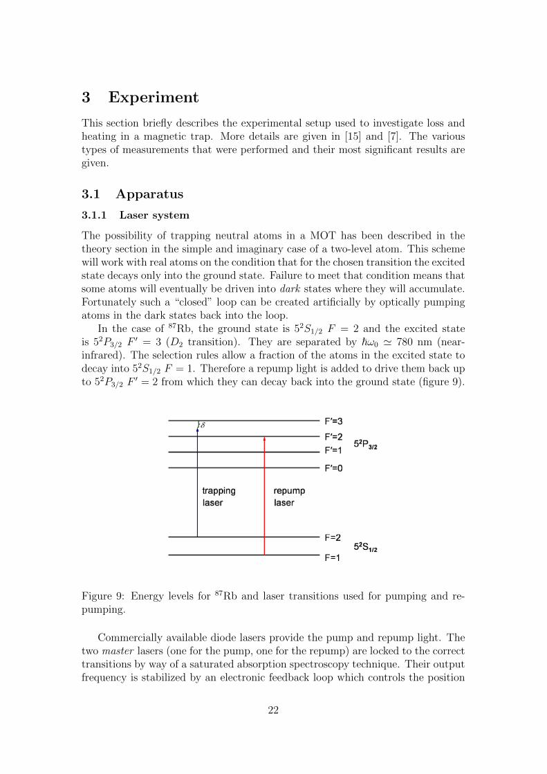
The possibility of trapping neutral atoms in a MOT has been described in thetheory section in the simple and imaginary case of a two-level atom. This schemewill work with real atoms on the condition that for the chosen transition the excitedstate decays only into the ground state. Failure to meet that condition means thatsome atoms will eventually be driven into dark states where they will accumulate.Fortunately such a “closed” loop can be created artificially by optically pumpingatoms in the dark states back into the loop.
In the case of 87Rb, the ground state is 52S1/2 F = 2 and the excited stateis 52P3/2 F
′ = 3 (D2 transition). They are separated by ~ω0 ' 780 nm (near-infrared). The selection rules allow a fraction of the atoms in the excited state todecay into 52S1/2 F = 1. Therefore a repump light is added to drive them back upto 52P3/2 F
′ = 2 from which they can decay back into the ground state (figure 9).
Figure 9: Energy levels for 87Rb and laser transitions used for pumping and re-pumping.
Commercially available diode lasers provide the pump and repump light. Thetwo master lasers (one for the pump, one for the repump) are locked to the correcttransitions by way of a saturated absorption spectroscopy technique. Their outputfrequency is stabilized by an electronic feedback loop which controls the position
22
of a diffraction grating placed outside the cavity. The diffracted light with thedesired frequency is re-injected into the cavity, saturating the gain medium andextinguishing all competing frequencies. This scheme provides very stable lightwith a narrow linewidth, but insufficient power for the creation of a MOT. There-fore this light is injected into slave diodes with a much higher power output. Again,injecting light of a given frequency forces the slave to emit at the same frequency[15].
The powerful, stable, narrow-linewidth light can then be driven through acousto-optic modulators (AOM) to adjust the frequency (for example detuning the lightfor the purposes of trapping). It is then split into three beams and sent in throughthe vacuum cell along three orthogonal axes. The correct circular polarization isobtained through a set of quarter-wave plates. Mirrors reflect the beams back tocomplete the MOT (the reflection conveniently changes σ+ light into σ− and viceversa).
3.1.2 Test chamber
The test chamber in which the MOT and magnetic trap are formed is a glass cellmeasuring 6× 1× 1 cm3
The ultra-high vacuum required to form a fair sized MOT or a long-lived mag-netic trap in that chamber is obtained through several pumps:
• an ion pump which uses combined electric and magnetic fields to ionize theatoms and accelerate them towards a solid electrode
• and chemical getter pumps that rely on chemical reactions to capture nitro-gen, hydrogen, oxygen, and methane.
Rubidium vapour can be released into the system by driving a current througha source. The current vaporizes the rubidium atoms contained in an alloy. Afterrefilling for a few minutes, the pressure decreases over the course of approximately12 hours as the pumps evacuate the extra rubidium atoms. As the pressure de-creases the pump becomes less efficient and the pressure ultimately stabilizes.
3.1.3 Imaging devices
The fluorescence from the MOT is collected by a lens and measured using a photo-diode. If the MOT density is not too large, this signal is proportional to the numberof atoms.
A CCD camera is also used to image the shape of the atom cloud. This is usefulwhen realigning the MOT beams, to make sure the MOT is stable and spherical.Flaring, bouncing and splitting of the MOT must be avoided to ensure a stablesignal, with a high signal-to-noise ratio.
23
3.2 Measuring losses
3.2.1 Experimental sequence
All experiments involving the magnetic trap start by loading atoms from the MOTinto the magnetic trap. This is simply done by turning off the lasers and increasingthe current in the magnetic coils (from 0.5 A to values between 1.5 A and 15A). Far-detuning the lasers before turning them off further cools the ensemble,increasing the efficiency of the transfer. If the repump laser is turned off beforethe pump, the pump will empty out the F = 2 ground state and all of the atomswill end up in F = 1. Conversely, if the pump beam is turned off first, atoms endup in the F = 2 state (figure 9). The experiments described in this report havebeen performed with 87Rb in the F = 1 state. Unless otherwise mentioned, thebackground gas is a mixture of 87Rb and 85Rb.
The magnetic trap is left to evolve for a given amount of time. The number ofatoms left in the trap is then measured by turning the lasers back on and doinga fluorescence measurement. Next, a baseline measurement is made by turningoff the magnetic field so that atoms leave the trap but the scattered laser lightbackground signal remains. Finally the MOT is refilled completely and anotherexperimental point can be taken (figure 10).
Figure 10: Diagram of a fluorescence curve as observed in a typical experiment.
The population in the magnetic trap is expressed as a fraction of the full MOTpopulation:
Since each trap depth U is linked to an angle θmin (equation (1.34)), the dependenceof the rate coefficient 〈σUv〉 on trap depth informs us on the angular dependence
24
of the differential cross-section [12, 13].If X refers to a species present in the background vapour,
Γ = nX〈σv〉X +∑
ni〈σv〉i (3.2)
where the first term corresponds to losses caused by collisions between trappedrubidium and background X and the second term refers to collisions with othergases that might be present in the background vapour (typically H2, CO, CH4 andN2).
The rate coefficient 〈σv〉X can be obtained as the slope of the plot of lossrate versus X density. Previous work at QDG involved measuring 〈σv〉Ar versustrap depth for rubidium-argon collisions. Argon was leaked into the system anda residual gas analyzer (RGA) was used to determine its pressure. For a numberof trap depths, loss rates were measured at various argon pressures. Very goodagreement with the theory was found [8].
However, rubidium pressure cannot be measured directly with an RGA. Indeed,rubidium atoms tend to stick to the stainless steel walls of the vacuum system. Asa consequence, pressure gradients form in the system, making a measurement ofthe pressure in the cell very difficult.
A possible proxy is the MOT’s loading rate, which is proportional to the back-ground rubidium pressure: R = αnRb. It can easily be fitted from fluorescencecurves as it is the initial slope of the MOT loading curve (equation (1.41)).Thedownside is that α is unknown and is liable to change when the MOT beams arereadjusted, an operation that must be done nearly daily. Nevertheless, by vaporiz-ing rubidium into the chamber and measuring loss rates (for various trap depths)as the pressure drops back down, one can obtain plots of the loss rate versus R,the slopes of which are 〈σv〉X/α. Finally we have the desired result, but scaled bya factor α. This means that when comparing with theory, α remains as a fittingparameter (figure 11).
Note that once α is known, a single MOT loading curve suffices to know thepressure. Unfortunately, as we have mentioned earlier, α is liable to change fromday to day. But there is another, simpler way of measuring background gas pres-sure.
3.2.3 Measuring pressure and trap depth
Equation (3.2) links loss rate, background gas density and trap depth (the ratecoefficient corresponds to a unique trap depth). If we are confident that theoret-ically calculated and experimentally measured rate coefficients agree, a loss ratemeasurement can be used to determine pressure (if the trap depth is known) ortrap depth (if the pressure is known).
25
Figure 11: Loss rate coefficient 〈σUv〉 versus trap depth U . The blue line is thetheoretical prediction for 300 K rubidium atoms colliding with static rubidiumatoms. The squares are experimental points, they have been scaled to best fit thetheoretical curve; the red and green points have been scaled separately.
Indeed, if the loss rates at various (known) trap depths are plotted against thecorresponding theoretical rate coefficients, according to equation (3.2) the pointsshould line up11 and the slope is the background rubidium density. The y-interceptcorresponds to the contribution of other gases to the loss rate.
Conversely, if the loss rate is measured for various pressures of X at a constant,unknown trap depth, the slope of the corresponding curve is 〈σv〉X , which givesus the trap depth. Note that this technique is very robust and works for all kindsof traps, as demonstrated by Janelle Van Dongen’s work at QDG [16].
3.3 Measuring heating
3.3.1 First attempts
A first order approach to the measurement of heating is to divide the trap intotwo energy bins and count the number of atoms in the lower and higher bins overtime.
Consider a trap of depth E1, and E0 an intermediate energy. Bin 0 coversenergies from 0 to E0 and bin 1 goes from E0 to E1. They contain respectively N0
and N1 atoms. The heated fraction is defined by:
HF =N1
N0 +N1
(3.3)
Experimentally, heated fraction measurements start by emptying the upper bin
11If∑ni〈σv〉i does not vary too much with trap depth, which is usually the case.
26
by setting the RF to ν0 = E0/h12. The trap is then left to evolve for some time
(the trap depth E1 is often set by using the RF knife at ν1 = E1/h during thattime). At the end of the run, either the RF is set at ν0 once more, or it isn’t. Inthe former case, the number of remaining atoms is N0, in the latter it is N0 +N1.
At first the frequency of the RF knife was swept between the desired cuttingfrequency and a high frequency, so as to empty out the high energy atoms faster.However this method gave noisy results, possibly because some atoms were ejectedfrom the trap and then flipped back in. Keeping the RF knife at a constantfrequency and waiting for the atoms with enough energy to cross the shell itdefines yields far better results. Actually, the precision of our measurements wasenhanced to the point that we could abandon the heated fraction technique andsample the entire energy distribution instead.
3.3.2 Probing the energy distribution
Using the RF at a frequency ν after having held atoms in the trap for a periodof time t will leave you only with atoms with energies below hν. This is pre-cisely the cumulative energy distribution (non-normalized) evaluated in hν, i.e.N(E = hν, t) if we reintroduce the quantities defined in section 1.3.3. By varyingν, the entire cumulative distribution can be sampled (figure 12).
Figure 12: Cumulative energy distribution in a 55 MHz deep trap after 0.4 s (bluesquares), 4.5 s (red circles) and 10 s (green triangles); either non-normalized (left)or normalized (right). Not only do the non-normalized distributions get smaller asatoms are lost from the trap, but their shape changes over time, as clearly shown bythe normalized distributions. The normalized curves shift towards larger energiesas time goes by, indicating heating.
The average energy per particle is E(t) = 1N(U,t)
∫ U0Eρ(E, t)dE. An integration
by part gives a convenient way of obtaining that energy from the data:
E(t) = U − 1
N(U, t)
∫ U
0
N(E, t)dE (3.4)
12This step is not absolutely necessary, its object is only to make heating more visible.
27
If the energy distribution is measured after various wait times, one can plot theaverage energy versus time. This curve appears to be linear, though we expect it
to curve off for longer times13. Its slope is what we will call the heating ratedE
dt.
As expected, the heating rate increases linearly with background rubidiumdensity (figure 13). The slope of these curves is what we will refer to as density-
normalized heating rate (1
nb
dE
dt). It is the equivalent, for heating, of the loss rate
coefficient.
Figure 13: Heating rate dEdt
versus background rubidium density nb for a 40 MHztrap (red circles) and a 60 MHz trap (blue squares). The lines are weighted linearfits. Heating increases linearly with the collision rate, and so with the backgroundgas density. This increase is faster for a deeper trap, as more collisions lead toheating, and less to loss.
As shown by figure 14, larger trap depths allow more heating as fewer collisionslead to loss.
To observe the effects of the atoms’ finite temperature on heating the initialtemperature of the atoms was varied. The initial energy distribution of the trappedatoms can be changed by using the RF knife to cut out the hotter part of thedistribution, leaving the remaining atoms with less energy on average. Anotherpossibility, suggested by the simulation, is to vary the length of time during whichthe coil current is being ramped when the atoms are loaded from the MOT intothe magnetic trap. If the magnetic field is turned on slowly after the lasers areturned off, the atoms have the time to move away from the centre of the trap andend up with more potential energy when the magnetic field is fully turned on, thus
13This is a result of the simulation, but it is obvious that heating cannot go on indefinitely asthe trap has a finite depth.
28
the distribution is hotter. On the contrary, ramping the magnetic field quicklyleads to a cooler initial distribution (figure 15).
Figure 14: Density-normalized heating rate 1nb
dEdt
versus trap depth U . Shallowertraps allow less heating to take place.
Figure 15: Cumulative energy distributions: either the magnetic field is crankedup instantly (blue squares), in which case the average energy is 8.5± 0.3 MHz, orit is ramped up in 50 ms (red circles) and the average energy is 15.4 ± 0.3 MHz.The faster the magnetic field is turned on, the less times atoms have to wanderaway from the centre of the trap, and the less potential energy they end up having.
29
Figure 16 shows that a trap that initially holds hot atoms cannot be heated asmuch as a trap with a colder initial distribution .
Figure 16: Density-normalized heating rate 1nb
dEdt
versus the initial average energyper atom. A warmer distribution heats up more slowly as atoms are more easilyexpelled from the trap.
Conclusion
Over the course of this internship, my colleagues and I have experimentally char-acterized loss and heating for an ensemble of cold atoms colliding with room-temperature atoms. In particular, we probed the energy distribution in the trapusing an RF knife and were able to detect its evolution over time.
Concurrently, we designed a direct simulation of the trap. Unlike the existenttheoretical models, the simulation takes the finite temperature of the trappedatoms into account. Both the experiments and the simulation showed that it wasnecessary to take finite temperature effects into consideration to describe heatingprecisely.
Comparison between numerical and experimental is currently under way. Weare hoping the two will concur and validate our approach.
Future work at QDG could involve:
• using argon as a background gas in order to have better control over itspressure,
• trying to replicate these results with 85Rb,
• probing the density distribution of the trapped atoms by using the RF knifein very short pulses, so as to take out atoms at a given position only,
30
• investigating losses from the MOT due to collisions between ground andexcited state atoms,
• linking loss rate and capture rate for a MOT,
• studying inelastic or reactive collisions,
• . . .
Research with cold atoms is a very active and fast-moving field. We hopethat our results can help others to better deal with limitations such as losses andheating, but we would also like to point out that they are not only hindrances,they are a rich subject of research in themselves.
References
[1] S. Bali, K.M. OHara, M.E. Gehm, S.R. Granade, and J.E. Thomas. Quantum-diffractive background gas collisions in atom-trap heating and loss. PhysicalReview A, 60(1):29–32, 1999. → pg. 16, 17, 19
[2] H.C.W. Beijerinck. Rigorous calculation of heating in alkali-metal traps bybackground gas collisions. Physical Review A, 61(3):33606, 2000. → pg. 16,17, 19
[3] G.A. Bird. Molecular gas dynamics and the direct simulation of gas flows.1994. Clarendon Press, Oxford. → pg. 12
[5] Claude Cohen-Tannoudji, Bernard Diu, and Franck Laloe. Mecanique quan-tique. Hermann, 1973. → pg. 7, 13, 14, 15
[6] D. Cook, W. M. Duckworth, M. S. Kaiser, W. Q. Meeker, and W. R. Stephen-son. Beyond Traditional Statistical Methods, chapter 2. 1999. → pg. 21
[7] David E. Fagnan. Study of collision cross section of ultra-cold rubidium usinga magneto-optic and pure magnetic trap, April 2009. Honour’s Thesis. → pg.7, 15, 22
[8] David E. Fagnan, Jicheng Wang, Chenchong Zhu, Pavle Djuricanin, Bruce G.Klappauf, James L. Booth, and Kirk W. Madison. Observation of quantumdiffractive collisions using shallow atomic traps. Phys.Rev.A., 80:022712, 2009.→ pg. 4, 16, 19, 25
[9] C.J. Foot. Atomic physics. Oxford University Press, USA, 2005. → pg. 10
[10] B.R. Johnson. The multichannel log-derivative method for scattering calcu-lations. J. Comp. Phys, 13:445–449, 1973. → pg. 15
31
[11] E. Majorana. Atomi orientati in campo magnetico variabile. Il Nuovo Cimento(1924-1942), 9(2):43–50, 1932. → pg. 6
[12] K.J. Matherson, R.D. Glover, D.E. Laban, and R.T. Sang. Absolutemetastable atom-atom collision cross section measurements using a magneto-optical trap. Review of Scientific Instruments, 78:073102, 2007. → pg. 25
[13] K.J. Matherson, R.D. Glover, D.E. Laban, and R.T. Sang. Measure-ment of low-energy total absolute atomic collision cross sections with themetastableˆ3 P 2 state of neon using a magneto-optical trap. PhysicalReview A, 78(4):42712, 2008. → pg. 25
[14] P. van der Straten and H. Metcalf. The quest for bec. Interactions in UltracoldGases: From Atoms to Molecules, pages 1–63. → pg. 7, 10
[15] Janelle Van Dongen. Simultaneous cooling and trapping of 6li and 85/87rb.Master’s thesis, UBC, December 2007. → pg. 22, 23
[16] Janelle Van Dongen, Chenchong Zhu, Gabriel Dufour, James L. Booth, andKirk W. Madison. Trap depth determination using residual gas collisions.Submitted to Phys. Rev. A. → pg. 17, 26