Chapter 3

Staged-Process Models:The Calculusof Finite Differences

5.1 INTRODUCTION

Chemical processing often requires connecting finite stages in series fashion.Thus, it is useful to develop a direct mathematical language to describeinteraction between finite stages. Chemical engineers have demonstrated con-siderable ingenuity in designing systems to cause intimate contact betweencountercurrent flowing phases, within a battery of stages. Classic examples oftheir clever contrivances include plate-to-plate distillation, mixer-settler systemsfor solvent extraction, leaching batteries, and stage-wise reactor trains. Thus,very small local driving forces are considerably amplified by imposition ofmultiple stages. In the early days, stage-to-stage calculations were performedwith highly visual graphical methods, using elementary principles of geometryand algebra. Modern methods use the speed and capacity of digital computa-tion. Analytic techniques to exploit finite-difference calculus were first publishedby Tiller and Tour (1944) for steady-state calculations, and this was followed bytreatment of unsteady problems by Marshall and Pigford (1947).

We have seen in Chapter 3 that finite difference equations also arise in PowerSeries solutions of ODEs by the Method of Frobenius; the recurrence relationsobtained there are in fact finite-difference equations. In Chapters 7 and 8, weshow how finite-difference equations also arise naturally in the numericalsolutions of differential equations.

In this chapter, we develop analytical solution methods, which have very closeanalogs with methods used for linear ODEs. A few nonlinear differenceequations can be reduced to linear form (the Riccati analog) and the analogousEuler-Equidimensional finite-difference equation also exists. For linear equa-tions, we again exploit the property of superposition. Thus, our general solu-tions will be composed of a linear combination of complementary and particularsolutions.

5.1.1 Modeling Multiple Stages

Certain assumptions arise in stage calculations, especially when contactingimmiscible phases. The key assumptions relate to the intensity of mixing and theattainment of thermodynamic equilibrium. Thus, we often model stages usingthe following idealizations:

• CSTR Assumption (Continuous Stirred Tank Reactor) implies that the compo-sition everywhere within the highly mixed fluid inside the vessel is exactlythe same as the composition leaving the vessel.

• Ideal Equilibrium Stage Assumption is the common reference to an "ideal"stage, simply implying that all departing streams are in a state of thermody-namic equilibrium.

As we show by example, there are widely accepted methods to account forpractical inefficiencies that arise, by introducing, for example, Murphree Stageefficiency, and so on.

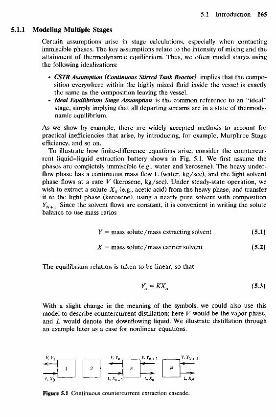
To illustrate how finite-difference equations arise, consider the countercur-rent liquid-liquid extraction battery shown in Fig. 5.1. We first assume thephases are completely immiscible (e.g., water and kerosene). The heavy under-flow phase has a continuous mass flow L (water, kg/sec), and the light solventphase flows at a rate V (kerosene, kg/sec). Under steady-state operation, wewish to extract a solute X0 (e.g., acetic acid) from the heavy phase, and transferit to the light phase (kerosene), using a nearly pure solvent with compositionYN+1. Since the solvent flows are constant, it is convenient in writing the solutebalance to use mass ratios

Y = mass solute/mass extracting solvent (5.1)

X = mass solute/mass carrier solvent (5.2)

The equilibrium relation is taken to be linear, so that

Yn = KXn (5.3)

With a slight change in the meaning of the symbols, we could also use thismodel to describe countercurrent distillation; here V would be the vapor phase,and L would denote the downflowing liquid. We illustrate distillation throughan example later as a case for nonlinear equations.

Figure 5.1 Continuous countercurrent extraction cascade.

A material balance on the nth stage can be written, since accumulation is nil(steady state)

LXn^ + VYn + 1 -LXn-VYn = O (5.4)

We can eliminate either X or Y, using Eq. 5.3. Since we are most concernedwith the concentration of the light product phase (Y1), we choose to eliminateX; hence,

(^)Yn-I + VYn + 1 - [^Yn -VYn = O (5.5)

Dividing through by V yields a single parameter, so we have finally,

Yn + 1 - (P + I)Yn+PYn^ = O (5.6)

where

This equation could be incremented upward (replace n with n + 1) to readilysee that a second order difference equation is evident

Yn+2-(p+ I)Yn + 1+/3Yn = O (5.7)

Thus, the order of a difference equation is simply the difference between thehighest and lowest subscripts appearing on the dependent variable (Y in thepresent case). Thus, we treat n as an independent variable, which takes on onlyinteger values.

5.2 SOLUTION METHODS FOR LINEAR FINITE DIFFERENCE EQUATIONS

It was stated at the outset that analytical methods for linear difference equa-tions are quite similar to those applied to linear ODE. Thus, we first find thecomplementary solution to the homogeneous (unforced) equation, and then addthe particular solution to this. We shall use the methods of UndeterminedCoefficients and Inverse Operators to find particular solutions.

The general linear finite difference equation of A:th order can be written justas we did in Section 2.5 for ODE

Yn+k + *k-i(n) • Yn+k_x + • • • +aQ(n)YH = f(n) (5.8)

It frequently occurs that the coefficients ak are independent of n and takeconstant values. Moreover, as we have seen, the second order equation arisesmost frequently, so we illustrate the complementary solution for this case

Yn+2+ Ci1Yn + 1+U0Yn = O (5.9)

Staged processes usually yield a negative value for U1, and by comparing withthe extraction battery, Eq. 5.7, we require ax = -(/3 + 1) and a0 = p.

5.2.1 Complementary Solutions

In solving ODE, we assumed the existence of solutions of the form y =Aexp(rx) where r is the characteristic root, obtainable from the characteristicequation. In a similar manner, we assume that linear, homogeneous finitedifference equations have solutions of the form, for example, in the previousextraction problem

Yn=A(T)" (5.10)

where A is an arbitrary constant obtainable from end conditions (i.e., wheren = 0, n = N + 1, etc.). Thus, inserting this into this second order Eq. 5.9, with^ 1 = -(/3 + 1) and a0 = /3 yields the characteristic equation for the extractionbattery problem

r2 - (/3 + \)r + /3 = 0 (5.11)

This implies two characteristic values obtainable as

(ff + l) + y/(/3 + l ) 2 - 4 f f (p + 1) ± Q - 1)ri,2 — 2 ~~ 2 w* l z /

which gives two distinct roots

T1=JS; r 2 = l

Linear superposition then requires the sum of the two solutions of the form inEq. 5.10, so that

Yn =A(rY)n + B(r2)n= A(f$)n + B(I)" (5.13)

We can now complete the solution for the extraction battery. Thus, taking thenumber of stages TV to be known, it is usual to prescribe the feed composition,X0, and the solvent composition YN+1. From these, it is possible to find theconstants A and B by defining the fictitious quantity F0 = KX0; hence

KX0 = A(/3)° + B(I)0 =A + B (5.14)

YN+1=A(P)N+1+B (5.15)

so we can solve for A and B

A = T - ^ ' 1 (5-16)and

P _ YN+I ~ KXOPN+1

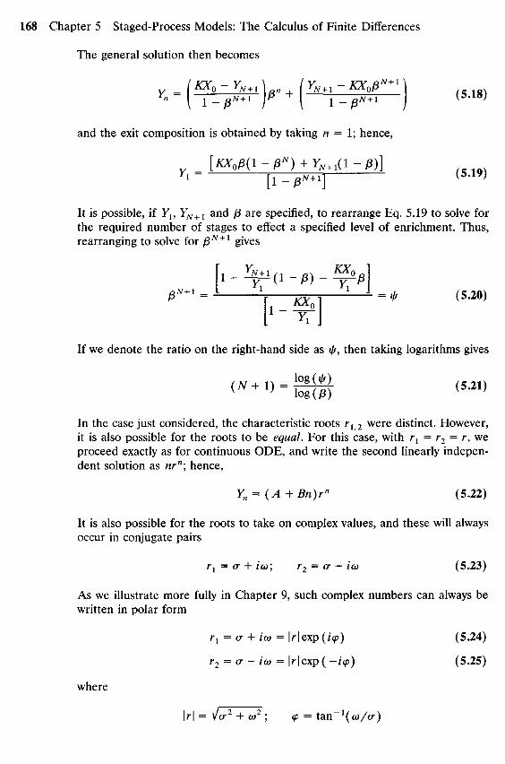
The general solution then becomes

Yn = (*f°_~^r)r + (YN+\~_™fr) (5-18)

and the exit composition is obtained by taking n = 1; hence,

[Xy0JB(I- g" ) + F N + 1 ( I -P)]yi - [l-j8"+1] ( }

It is possible, if Y1, YN+1 and /3 are specified, to rearrange Eq. 5.19 to solve forthe required number of stages to effect a specified level of enrichment. Thus,rearranging to solve for fiN+l gives

^ " = \ SI = * (5'20)

L1" YAIf we denote the ratio on the right-hand side as ifj, then taking logarithms gives

In the case just considered, the characteristic roots rl2 were distinct. However,it is also possible for the roots to be equal. For this case, with rx = r2 = r, weproceed exactly as for continuous ODE, and write the second linearly indepen-dent solution as nrn\ hence,

Yn = (A +Bn)rn (5.22)

It is also possible for the roots to take on complex values, and these will alwaysoccur in conjugate pairs

rx = a + ico; r2 = a — ico (5.23)

As we illustrate more fully in Chapter 9, such complex numbers can always bewritten in polar form

rx = a + io) = \r\exp(i(p) (5.24)

r2 = a - ico = \r\exp(—i<p) (5.25)

where

\r\ = V7O-2 + a)2 ; <p = t a n " 1 (co/a)

Here, |r| is called the modulus, and <p is the phase angle. It is now clear that theEuler formula can be used to good effect

| r | exp( i» =|r |[cos(?) +/sin(<p)] (5.26)

so we insert the two complex roots and rearrange to get

Yn = \r\n[ A cos (n<p) +B sin (n<p)] (5.27)

since

exp (in<p) = cos (n<p) + / sin (n<p)

EKMiPLESJ

It is desired to find the required number of ideal stages in the extractioncascade illustrated in Fig. 5.1. Take the feed-to-solvent ratio (L/V) andequilibrium distribution constant (K) to be unity, then /3 = L/(KV) = 1. Puresolvent is specified, so YN+1 = 0 kg solute/kg solvent, and the feed is X0 = 1 kgsolute/kg carrier. It is desired to produce a rich extract product such thatY1 = 0.9 kg solute/kg solvent.

This problem can be solved by classical methods, using graphical constructionas illustrated in Fig. 5.2. The stage-to-stage calculations require linear connec-tions between equilibrium line (i.e., departing streams) and operating line. Thepassing streams are related by way of a material balance between any stage nand the first stage, and this relationship is called the operating line; thus, we

Figure 5.2 Graphical stage-to-stage calculations.

Equilibrium line

Operating line

Yn

write the material balance:

VYn + 1 +LX0 = VY1 + LXn (5.28)

and rearrange to find Yn + 1 = f(Xn) which is the operating line

Yn + 1-(y)xn + (Y1-X0^) (5.29)

with slope L/ V and intercept (Y1 - X0 L/ V). This line is plotted along withthe equilibrium curve (Yn = KXn) in Fig. 5.2, and stages are stepped-off asillustrated to yield N = 9 stages.

A direct computation could have been performed using Eq. 5.21. However,since /3 = 1, a difficulty arises, since

log(<A)/log(/3) = log(l)/ log(l) = 0/0

which is indeterminate. To resolve this difficulty, we can perform the limitingoperation

<"+1J-SSw- (5-30)

To perform this limit, we can use the series expansion for logarithms

log (x) = (x - 1) - \(x - I)2 + • • • (5.31)

so for x ~ 1, use the first term to get

(N + 1) = hm T^ TT (5.32)

This gives a finite limit, since (/3 - 1) cancels and we finally get

valid for /3 = 1. Inserting the given parameters yields

( N + I ) = ( 1 _ 1Q 9 ) = 1 0 - : N = 9 (5.34)

We could also have resolved this indeterminacy using L'Hopital's rule.In Section 2.4.2, we illustrated how to reduce a certain class of variable

coefficient ODE to an elementary constant coefficient form; such equationforms were called Equidimensional or Euler equations. The analog of this also

exists for finite difference equations; for example,

(n + 2)(n + I)Yn+2+A(n + I)Yn + 1 +BYn = O (5.35)

This can be reduced to constant coefficient status by substituting

Yn = TTT ( 5 - 3 6 )

hence, we have in terms of z

Zn+2+Azn + 1+Bzn = O (5.37)

EMMPlMSJ

Find the analytical solution for an in the recurrence relation given in Eq. 3.9,subject only to the condition aQ is different from 0

«n+2(» + 2)(« + 1) - 2an + l(n + 1) + an = 0 (5.38)

As suggested in Eq. 5.36, let

a" = Sf (5 J 9>so we get a relation for an

an+2-2an + 1 + an = 0 (5.40)

Now, assume a solution for this constant coefficient case to be

an=Arn (5.41)

so the characteristic equation is

r2 - Ir + 1 = 0 (5.42)

Hence, we have equal roots: rx = r2 = 1. According to Eq. 5.22, the solution is

an = (A + Bn)rn = {A + £n) (5.43)

and so from Eq. 5.38,

{A +Bn)an = ~—j[\—" (5-44)

Now, the only boundary condition we have stipulated is that a0 is different from0, so one of the constants A or B must be set to zero. If we set A = O, then we

would have

But when n = 0, then (-1)! = ». This says «0 = 0. Thus, we must set B = 0and write #„ = A/n\. Now, since ^0 is different from zero, set n = 0 to see that4̂ = fl0, since 0! = 1. This reproduces the result given by Eq. 3.10, with r = 1

«n - S (5.46)

5.3 PARTICULAR SOLUTION METHODS

We shall discuss two techniques to find particular solutions for finite differenceequations, both having analogs with continuous ODE solution methods:

1. Method of Undetermined Coefficients2. Method of Inverse Operators

A Variation of Parameters analog was published by Fort (1948).

5.3.1 Method of Undetermined Coefficients

Under forced conditions, the constant coefficient, second order finite differenceequation can be written, following Eq. 5.8

Yn+2+ O1Yn + 1 +Ci0Yn =f(n) (5.47)

where f(n) is usually a polynomial function of n. Thus, if the forcing function isof the form

f(n) =b0 + bxn + b2n2 + • • • (5.48)

then the particular solution is also assumed to be of the same form

Ynp = a0 + Ct1H + a2n

2 + • • • (5.49)

where at are the undetermined coefficients. The particular solution is insertedinto the defining equation, yielding a series of algebraic relations obtained byequating coefficients of like powers. Difficulties arise if the forcing function hasthe same form as one of the complementary solutions. Thus, linear indepen-dence of the resulting solutions must be guaranteed, as we illustrated earlier,for example, in Eq. 5.22 (for the occurrence of equal roots). We illustrate themethod by way of examples in the following.

Find the particular solution for the forced finite difference equation

Vn + X-Iyn- 3yn^ = (n + l) (5.50)

Inserting an assumed solution of form

yn = a0 + axn (5.51)

into Eq. 5.50 yields

a0 + Ot1(H + 1) - 2(a0 + OL1Ti) - 3[a0 + ax(n - I)] = n + 1 (5.52)

Equating coefficients of unity and rc gives, first for coefficient of unity

ao + ai ~ 2a0 ~ 3a0 + 3«! = 1 (5.53)

hence,

4«! - 4a0 = 1 (5.54)

Next, coefficients of n give

^1 — 2 ^ 1 — 3 a t = 1 .*.«! = — -T (5.55)

We can now solve Eq. 5.54 for a0

aQ=-\ (5.56)

The particular solution can now be written

ypn = -\~\n (5.57)

To check linear independence with the complementary parts, first find thecharacteristic roots from the homogeneous equation to see

r2 - Ir - 3 = 0 .\r1>2 = 3 , - 1 (5.58)

ycn=A(3)n + B(-l)n (5.59)

and these are obviously independent of the particular solutions. The generalsolution is written as before: yn = yc

n + y%. The coefficients A and B are foundfor the general solution using end conditions.

EKAMPLE SA

Repeat the previous problem, except the forcing function, f(n) = (3)n.It is clear that an assumed solution of the form

ypn = «(3)" (5.60)

will not be linearly independent of one of the complementary solutions.

Therefore, we assume a solution form, which is clearly independent

yZ = pn(3)" (5.61)

Inserting this gives

p(n + 1)3" + 1 - 2pn3n - 3p(n - I)S""1 = 3n (5.62)

Dividing through by 3" gives

3p(n + 1) - lfin - p(n - 1) = 1 (5.63)

Equating coefficients of unity allows the undetermined coefficient P to be found

3/3 + /3 = 1 :.p = \ (5.64)

Coefficients of n are exactly balanced, since

3Pn - ipn -IPn = O (5.65)

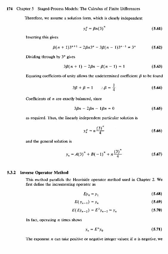
as required. Thus, the linearly independent particular solution is

yZ = n&- (5.66)

and the general solution is

yn=A(3)"+B(-l)" + n&- (5.67)

5.3.2 Inverse Operator Method

This method parallels the Heaviside operator method used in Chapter 2. Wefirst define the incrementing operator as

Ey0 = yx (5.68)

E(yn-l)=yn (5.69)

E(Eyn_2)=E2yn_2=yn (5.70)

In fact, operating n times shows

yn = EnyQ (5.71)

The exponent n can take positive or negative integer values; if n is negative, we

increment downward. The equivalent of Rule 1 in Chapter 2 for arbitrary c is

Ecn = c n + l =ccn ^ j 2 )

Emcn = cm+n = ^n (5 73)

and as before, for any polynomial of E, Rule 1 is

P(E)cn =P(c)cn (5.74)

This has obvious applications to find particular solutions when f(n) = cn. Theanalogous form for Rule 2 is

P(E)(c"fn)=c"P(cE)fn (5.75)

Here, we see that cE replaces E. This product rule has little practical value inproblem solving.

Thus, we can rewrite Eq. 5.47 as

(E2 + axE + aQ)yn=f(n) (5.76)

Now, if f(n) takes the form Kc", then we can solve directly for the particularsolution

yn = T^—^r—^Kc" (5.77)[E + Ci1E + a0)

With the usual provision that the inverse operator can be expanded in series, wehave, using Rule 1,

provided c2 + a{c + a0 is different from zero.

EK4MPLM5.5

Find the particular solution for

y n + 2 - 2 y n + l-8yn = e" (5.79)

Writing in operator notation, we have in one step

vp = e" = e" (5 8(My» [E2-2E-8] [e2-2e-8] ( '

This would have required considerably more algebra using the method ofundetermined coefficients. To check for linear independence, the roots of the

homogeneous equation are

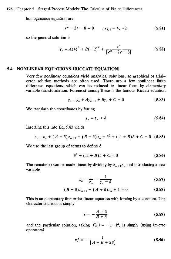
r2 - Ir - 8 = 0 :.rl2 = 4, - 2 (5.81)

so the general solution is

yn=A(4)"+B(-2r+[e2_e;e_8] (5.82)

5.4 NONLINEAR EQUATIONS (RICCATI EQUATION)

Very few nonlinear equations yield analytical solutions, so graphical or trial—error solution methods are often used. There are a few nonlinear finitedifference equations, which can be reduced to linear form by elementaryvariable transformation. Foremost among these is the famous Riccati equation

yn + iyn + Ayn + 1 + Byn + C = 0 (5.83)

We translate the coordinates by letting

yn = zn + 8 (5.84)

Inserting this into Eq. 5.83 yields

Zn + 1Zn + (A + 8)zn + l + (B + 8)zn + 82 + (A + B)8 + C = 0 (5.85)

We use the last group of terms to define 8

82 + (A+B)8 + C = 0 (5.86)

The remainder can be made linear by dividing by Zn + 1Zn and introducing a newvariable

(B + 8)vn+1 + (A +S)Vn + 1 = 0 (5.88)

This is an elementary first order linear equation with forcing by a constant. Thecharacteristic root is simply

and the particular solution, taking f(n) = — 1 • 1", is simply (using inverseoperators)

"•'--[A+B + 28] {5M)

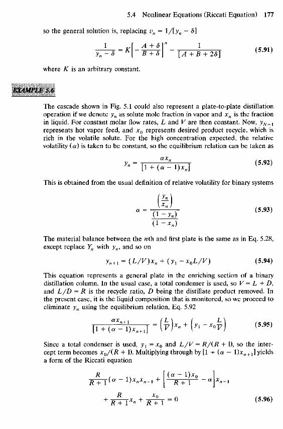
so the general solution is, replacing Vn = l/[yn — 8]

J-^8 -K[-TTS\ ~ [A +B + 28] ( 5 '9 1 )

where K is an arbitrary constant.

EMMPLM SJ

The cascade shown in Fig. 5.1 could also represent a plate-to-plate distillationoperation if we denote yn as solute mole fraction in vapor and Xn is the fractionin liquid. For constant molar flow rates, L and V are then constant. Now, yN+l

represents hot vapor feed, and xQ represents desired product recycle, which isrich in the volatile solute. For the high concentration expected, the relativevolatility (a) is taken to be constant, so the equilibrium relation can be taken as

This is obtained from the usual definition of relative volatility for binary systems

- - -tk (5-'3)(l-*n)

The material balance between the nth and first plate is the same as in Eq. 5.28,except replace Yn with yn, and so on

Vn + I = (WV)Xn+ (V1-X0LZV) (5.94)

This equation represents a general plate in the enriching section of a binarydistillation column. In the usual case, a total condenser is used, so V = L + D,and L/D = R is the recycle ratio, D being the distillate product removed. Inthe present case, it is the liquid composition that is monitored, so we proceed toeliminate yn using the equilibrium relation, Eq. 5.92

Since a total condenser is used, yx = X0 and L/V = R/(R + 1), so the inter-cept term becomes xo/(R + 1). Multiplying through by [1 + (a - D*n + 1] yieldsa form of the Riccati equation

JTTT (* " l)XnXn + l + [ ^ + !*° - aj*n + l

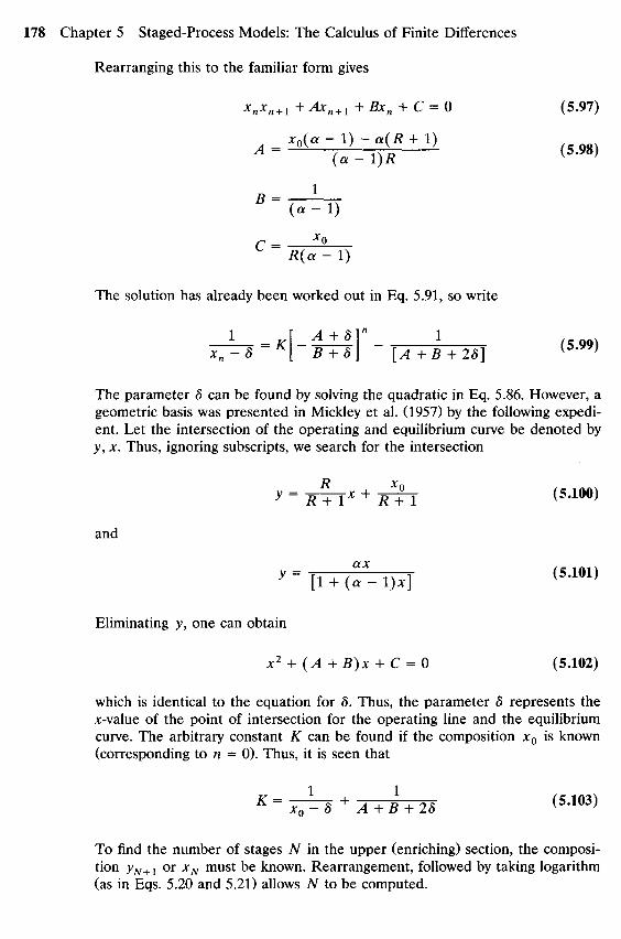
Rearranging this to the familiar form gives

xnxn + 1+Axn+1+Bxn + C = 0 (5.97)

x o ( « - I ) - « ( * + !)A ~ (a-I)R ( 5 > 9 8 )

C= ^R(a - 1)

The solution has already been worked out in Eq. 5.91, so write

1 =K\ A + 8]n 1Xn -8

A [ B + «] [ , 4 + 5 + 2S] l '

The parameter 5 can be found by solving the quadratic in Eq. 5.86. However, ageometric basis was presented in Mickley et al. (1957) by the following expedi-ent. Let the intersection of the operating and equilibrium curve be denoted byy, x. Thus, ignoring subscripts, we search for the intersection

y = TTFT* + TTTT (5'10°)

and

y - [i + C«-Dx] (5-101)

Eliminating y, one can obtain

x2 + (A + B)x + C = O (5.102)

which is identical to the equation for 8. Thus, the parameter 8 represents thejc-value of the point of intersection for the operating line and the equilibriumcurve. The arbitrary constant K can be found if the composition xQ is known(corresponding to n = 0). Thus, it is seen that

K = —^-=• + A , p , „ (5.103)x0 - 8 A + B + 28 v '

To find the number of stages N in the upper (enriching) section, the composi-tion yN+x or xN must be known. Rearrangement, followed by taking logarithm(as in Eqs. 5.20 and 5.21) allows TV to be computed.

5.5 REFERENCES

1. Fort, T. Finite Differences and Difference Equations in the Real Domain. OxfordUniversity Press, New York (1948).

2. Foust, A. S., L. A. Wenzel, C. W. Clump, L. Mans, and L. B. Andersen. Principles ofUnit Operations, p. 117, John Wiley & Sons, Inc., New York (1980).

3. Marshall, W. R., and R. L. Pigford. The Application of Differential Equations toChemical Engineering Problems. University of Delaware, Newark, Delaware (1947).

4. Mickley, H. S., T. K. Sherwood, and C. E. Reid. Applied Mathematics in ChemicalEngineering. McGraw Hill, New York (1957).

5. Pigford, R. L., B. Burke and D. E. Blum. "An Equilibrium Theory of the ParametricPump," Ind. Eng. Chem. Fundam., 8, 144 (1969).

6. Tiller, F. M., and R. S. Tour, "Stagewise Operations—Applications of the Calculus ofFinite Differences to Chemical Engineering," Trans. AIChE, 40, 317-332 (1944).

5.6 PROBLEMS

5.I2. Find the analytical solutions for the following finite difference equations

O) yn+3 ~ 3yn + 2 + 2yn + 1 = 0

(b) yn+3 ~ 6 y n + 2 + Hyn + 1 - 6yn = 0

(c) yn+2yn = yl+\

Hint: Use logarithms

(d) Rxn_x-Rxn = vsxn

when

* o - s

is initial state.5.2*. A continuous cascade of stirred tank reactors consists of TV tanks in series

as shown below.

The feed to the first tank contains C0 moles/cc of component A. Eachtank undergoes the irreversible reaction A -> B so that the reaction rateis Rn = kCn (moles/cc/sec). The volume rate of flow in the cascade isconstant at a value L (cc/sec).

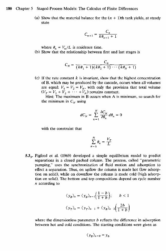
(a) Show that the material balance for the (n H- l)th tank yields, at steadystate

c c"n + 1 kfi + 1

where On = Vn/L is residence time.(b) Show that the relationship between first and last stages is

C = £>N (IcO1 + l)(fcfl2 + I ) " " (k0N + 1)

(c) If the rate constant k is invariant, show that the highest concentrationof B, which may be produced by the cascade, occurs when all volumesare equal: V1 = V2 = VN, with only the provision that total volume(VT = V1 + V2 + • • • + VN) remains constant.

Hint: The maximum in B occurs when A is minimum, so search forthe minimum in CN using

dCN= E ^dOn = On = \ n

with the constraint that

5.33. Pigford et al. (1969) developed a simple equilibrium model to predictseparations in a closed packed column. The process, called "parametricpumping," uses the synchronization of fluid motion and adsorption toeffect a separation. Thus, on upflow the column is made hot (low adsorp-tion on solid), while on downflow the column is made cold (high adsorp-tion on solid). The bottom and top compositions depend on cycle numbern according to

{yB)n-{yB)n-\\^y b<\

(yT)n = (yT)n-\ + (yB)n-*y I + ^ )

where the dimensionless parameter b reflects the difference in adsorptionbetween hot and cold conditions. The starting conditions were given as

(yB\=o = y0

Show that the separation factor for this process is

(yT>n /„ , 2b \(l+b\" (l + b\2 .

<>r>2-yo( i + T T F )

Is the separation factor bounded as n -> oo?5.4*. A gas-liquid chemical reaction is carried out in a cascade of shallow

bubble columns, which are assumed to be well mixed owing to the mixingcaused by gas bubbles. Each column contains H moles of liquid com-posed mainly of inert, nonvolatile solvent with a small amount of dis-solved, nonvolatile catalyst. Liquid does not flow from stage to stage. Puregas A is fed to the first column at a rate G (moles/sec). The exit gasfrom stage one goes to stage two, and so on. On each stage, some Adissolves and reacts to form a volatile product B by way of the reversiblereaction

A^B

A linear rate law is assumed to exist for each pathway. The B formed byreaction is stripped and carried off by the gas bubbling through the liquidmixture. Overall absorption, desorption efficiencies are predictable usingMurphree's vapor rule

A AV 1 — V/7 — yn — \ Jn

A y<t-,-{?ty

yB , -yB

B~ y?-i-(ynB)*

where the equilibrium solubilities obey Henry's law

{yBnf = rnBxB

n

Here, yn and Xn denote mole fractions, for the nth stage, and in thevapor phase, only A and B exist, so that y£ + y% = 1.(a) The moles of A or B lost to the liquid phase can be represented in

terms of stage efficiency; thus, for component A

GW-!-yf) = GEA[y^x - (y^)*] = GEA{y?_x-mAxf)

Write the steady-state material balances for the liquid phase and show

that

where

1/ kBH\F \ GEA )

kBHAp ~mB + - ^ -

EB-EA

I kAH\( kBHA\ kBH I kAHA\

I A GEA ) \ B G I GEA \ A G I

(b) Find the relationship to predict y* as a function of n, where y£ = 1.(c) The statement of the problem implies mB ;̂ > m^ ( 5 is volatile)

EB > EA (volatiles have higher efficiencies), and kA> kB. Are thesethe appropriate conditions on physical properties to maximize produc-tion of Bl Compute the composition y£, leaving the 5th stage for thefollowing conditions:

mB = 10; mA = 1; -77 = 0.1 sec"1; EA = EB = 0.5;

/c^ = 2 sec"1; Zc5 = 1 sec

Ans: 0.925.53. A hot vapor stream containing 0.4 mole fraction ammonia and 0.6 mole

fraction water is to be enriched in a distillation column consisting ofenriching section and total condenser. The saturated vapor at 6.8 atmpressure (100 psia) is injected at a rate 100 moles/hour at the bottom ofthe column. The liquid distillate product withdrawn from the total con-denser has a composition 0.9 mole fraction NH3. Part of the distillate isreturned as reflux, so that 85% of the NH3 charged must be recovered asdistillate product.(a) Complete the material balance and show that xN = 0.096 (mole

fraction NH3 in liquid leaving Nth tray) and that the required refluxratio is R = 1.65.

(b) The NH3-H2O system is highly nonideal, and hence, the relativevolatility is not constant, so that the assumption of constant molaroverflow is invalid. Nonetheless, we wish to estimate the number ofideal stages necessary, using the single available piece of vapor-liquidequilibria data at 6.8 atm pressure: y(NH3) = 0.8 when Jc(NH3) = 0.2.This suggests a « 16. Use this information and the results fromExample 5.6 to find the required number of ideal stages (an enthalpy-composition plot shows that exactly two stages are needed).

5.63. Acetone can be removed from acetone-air mixtures using simple counter-current cascades, by adsorption onto charcoal (Foust et al. 1980). We wishto find the required number of equilibrium stages to reduce a gas streamcarrying 0.222 kg acetone per kg air to a value 0.0202 kg acetone per kgair. Clean charcoal (X0 = 0) enters the system at 2.5 kg/sec, and the airrate is constant at 3.5 kg/sec. Equilibrium between the solid and gas canbe taken to obey the Langmuir-type relationship

Y - KXn - / r - n sr" " 1 + KXn ' A " u '*

whereYn = kg acetone/kg airXn = kg acetone/kg charcoal

(a) Write the material balance between the first stage (where X0 enters)and the nth stage, and use the equilibrium relationship to derive thefinite difference equation for Xn.

(b) Rearrange the expression in part (a) to show that the Riccati equationarises

XHXn + l+AXn + l+BXH + C = 0

What are the appropriate values for A9 B, and C?(c) Use the condition X0 = 0 (clean entering charcoal) to evaluate the

arbitrary constant in the general solution from part (b) and thus obtaina relationship to predict Xn = f(n).

(d) Use an overall material balance to find XN and use this to calculatethe number of equilibrium stages (AO required.

Ans: (d) 3.5 stages