2016

47

96 (3)STATISTIKA

Abstract

An important task in econometric modelling is to determinate the integration order of analysed time series through unit root tests. Statistical theory offers a wide range of tests where the most common are Dickey-Fuller tests, Phillips-Perron test, KPSS test, and their modifications ADF-GLS test and Ng-Perron test. The choice of an appropriate one depends primarily on a subjective judgement of the analyst. If we wish to avoid the sub-jective choice, we need to find an objective criterion that clearly defines which test is the most suitable for spe-cific types of time series. The goal of the article is to answer this question by a simulation study and to provide the recommendations which test is possible to use. The conclusions will be applicable for time series of lengths T = 25, ..., 500 and positive values of the autoregressive parameter AR(1).

Selection of Unit Root Test on the Basis of Lengthof the Time Series and Value of AR(1) ParameterMarkéta Arltová1 | University of Economics, Prague, Czech RepublicDarina Fedorová2 | IBM, Prague, Czech Republic

IntroductIon Statistics and econometrics use a single-equation or multi-equation regression models of time series for modelling economic variables and their interrelations. These models are based on the Box and Jenkins methodology (Box, Jenkins, 1970) and the fundamental assumption for their use is time series stationarity or their linear combinations stationarity in the case of multi-equation models. In practice, however, this condition is often not met because most of economic time series are non-stationary. These time series are denoted as integrated of order d when they are after the d-differentiations stationary.

Therefore, analytic models construction requires identification of the order of integration or the or-der of differentiation d. Econometrists employ several approaches to determine this order. The simplest method is an assessment of the time series graphs. The original time series is compared with time series

Keywords

Unit root test, augmented Dickey-Fuller test, Phillips-Perron test, KPSS test, ADF-GLS test,

NGP test, simulation, power of test, time series analysis

JEL code

C12, C15, C22, C51

1 Faculty of Informatics and Statistics, Nám. W. Churchilla 4, 130 67 Prague 3, Czech Republic. Corresponding author: e-mail: marketa.arltova@vse.cz.

2 IBM Czech Republic, V Parku 2294/4, 148 00 Prague 4, Czech Republic. E-mail: darina.fedorova@cz.ibm.com.

AnAlyses

48

of the first and second differences. Although this method has a subjective character, it is very effective in many cases, especially for experienced analysts. The shape of sample autocorrelation (ACF) and par-tial autocorrelation (PACF) functions (Box, Jenkins, 1970) is another simple method providing sufficient results. If the ACF is slowly decreasing, roughly at a linear rate, the PACF has a very high first value, the time series should be differentiated (the assumption is, that the time series does not contain the out-liers, whose presence can change the shape of both functions and it is necessary to remove it before the analysis). In case the time series is classified as non-stationary, then its first differences are analysed. Simi-larly, if the time series of first differences is non-stationary, the time series of second differences is analysed. The above approach, however, suffers by the over-differencing risk. Therefore, it is convenient to approach this problem formally and to use appropriate statistical tests to determine the order of differentiation.

The determination and verification of the order of integration is a quite wide area that includes an extensive list of tests known as unit root tests, where the most commonly used are Dickey and Fuller’s DF-test and ADF test (Dickey and Fuller, 1979), Phillips-Perron test (Phillips and Perron, 1988), KPSS test (Kwiatkowski, Phillips, Schmidt and Shin, 1992), also less frequently used ADF-GLS test (Elliot, Rothenberg and Stock, 1996) and NGP test (Ng and Perron, 1995 and 2001).

Consequently, there is a wide range of unit root tests that are usually integrated in statistical and econo-metric software. A question the analysts face is which one of them should be used as the most suitable test for the respective time series. The aim of this article is to solve this dilemma and advise which one of them to use under specific criteria. The recommendations concluded from this article are suitable for short and medium-long time series of lengths from 25 to 500 values and for positive values of parameter

of the autoregressive process AR(1).

1 rEVIEW oF SELEctEd unIt root tEStS1.1 dickey-Fuller tests (dF test and AdF test)Dickey-Fuller test (Dickey, Fuller, 1979) is one of the best known and most widely used unit root tests. It is based on the model of the first-order autoregressive process (Box, Jenkins, 1970):

(1)

where is the autoregression parameter, εt is the non-systematic component of the model that meets the characteristics of the white noise process.

The null hypothesis is , i.e. the process contains a unit root and therefore it is non-stationary, and is denoted as I(1), alternative hypothesis is , i.e. the process does not contain a unit root and is stationary, I(0).

To calculate the test statistic for DF test, we use an equation that we get if yt–1 is subtracted from both sides of the equation (1):

(2)

where . The test statistic is defined as:

(3)

where is a least square estimate of and is its standard error estimate. Under the null hypothesis this test statistic follows the Dickey-Fuller distribution, critical values for this distribution were obtained by a simulation and have been tabulated in Dickey (1976) and Fuller (1976).

2016

49

96 (3)STATISTIKA

Model (1) can be expanded by a constant or a linear trend:

(4)

(5)

In the case when a non-systematic component in DF models is autocorrelated, so-called Augmented Dickey-Fuller test is constructed (Dickey, Fuller, 1981). Model (1) is then transformed as:

(6)

and the following equation is used to calculate the test statistic of the ADF test:

(7)

A practical problem of this test is the choice of lags p. The next steps are the same as in the case of DF test. Schwert (1989) suggests choosing the maximum lag pmax = 12(T/100)1/4, because if p is too low, the test will be affected by autocorrelation and if p is too large, the power of test will be lower. Model (6) can be expanded by a constant, or linear trend as well. Then, tests based on the following model are used:

, (8)

where , for p = 0, 1, contains deterministic parts of the models mentioned above.

The limiting distribution of test statistics is identical with the distribution of DF test statistics and for T → ∞ is tabulated in Dickey (1976) and MacKinnon (1991).

1.2 Phillips-Perron test (PP test)In the unit root testing of time series generated by the process with autocorrelated and heteroscedastic non-systematic component, there is often a problem of selection of lag p in the regression model. Phillips and Perron (1988) were dealing with this problem and instead of describing the autocorrelation structure of the generating process by the corresponding autocorrelation models, they used standard Dickey-Fuller test with non-parametrically modified test statistics.

This test is also based on the models (1), (4) and (5) with the difference that the linear trend in the last model is replaced by a centred time variable.

Nevertheless, the next steps differ from Dickey-Fuller tests. This test is not using the differentiated equations for the test statistics calculation, but it derives it directly from the equations (1), (4) and (5).

The test statistics Z for model with a constant are written as follows (Pesaran, 2015):

(9)

AnAlyses

50

, (10)

where:

,

tDF is the test statistics of DF test, sT2 is the OLS estimator of the non-systematic component variance,

is the maximum likelihood estimator of the non-systematic component covariance and q is a num-ber of lag of covariates.

If εt is not autocorrelated, then , the limiting distribution of the test statistics t is therefore not dependent on autoregressive parameters of εt process. The test statistics Z are consequently reduced to tDF test statistics. Dickey-Fuller test is thus a special case of non-parametric tests.

1.3 AdF-GLS testADF-GLS test, also known as ERS test (Elliot, Rothenberg and Stock, 1996), is another modification of Augmented Dickey-Fuller test. Before the unit root testing, the ADF-GLS test utilizes the detrending transformation (i.e. transformation that removes trend from time series).

The constant in model (4) is estimated based on the generalised least squares method (GLS) using the transformation:

(11)

where 3 based on the equation:

(12)

Subsequently, parameter is estimated by the least squares method and used to remove constant from the time series yt

(13)

In the last step, the ADF test is calculated based on the transformed time series given by:

(14)

3 The value = –7 (resp. –13.5, in the case of a model with a linear trend) was deduced for α = 0.05 by Elliot, Rothenberg and Stock (1996) based on power envelope. For given T and when the relevant deterministic components are present the power envelope in this point reaches 50% (i.e., that the tests are optimal at the 50% power).

2016

51

96 (3)STATISTIKA

The trend in models with the linear trend is estimated by GLS. Transformation (11) is extended by z1 = 1, zt = t − ρ(t − 1), where ρ = 1 + /T, where = −13.5. Estimates of parameters are calculated based on equation:

(15)

and estimated parameters 0 and 1 are then used to remove trend from the time series yt

(16)

Finally, the ADF test is applied on the transformed time series, i.e. the test statistic is obtained from the following equation:

(17)

The critical values for the ADF-GLS test obtained on the basis of simulation in Elliot, Rothenberg and Stock (1996) show that for models without constant they are the same as in the case of the ADF test. For the remaining models, critical values of the ADF-GLS test are used as indicated in Elliot, Rothen-berg and Stock (1996) as well.

1.4 nGP testNg and Perron (1995, 2001) built on detrended data yt

* obtained from the ADF-GLS test and modified the Phillips-Perron PP test.

Based on the equation (8) the test uses test statistics Z from the PP test that had been modified by Ng and Perron into form:

(18)

(19)

(20)

where , and marked as M tests.

Although the NGP test is considered as an effective modification of unit root tests, it is not included in many statistical software.

AnAlyses

52

1.5 KPSS testAll the tests mentioned above are testing the null hypothesis that the time series yt is integrated of order one, I(1). The opposite case, i.e. testing the null hypothesis that the time series yt is I(0), is described by the KPSS test (Kwiatkowski, Phillips, Schmidt and Shin, 1992).

Kwiatkowski, Phillips, Schmidt and Shin built on the idea that the time series is stationary around a deterministic trend and is calculated as the sum of a deterministic trend, random walk and stationary random error. It is based on model:

(21)

where , for p = 0, 1, contains deterministic parts of the model (constant or deterministic

trend), εt are iid N(0, σε2), rt is a random walk with variance σu

2 and ut are iid N(0, σu2).

KPSS test is based on LM test of the hypothesis that the random walk has a zero variance, i.e. H0: σu

2 = 0, which means that rt is a constant, against the alternative H1: σu2 > 0. The test statistic is written as:

(22)

where T, and is the estimate of variance of process εt from the equation

(21). Critical values were derived by a simulation and are listed in Kwiatkowski, Phillips, Schmidt and Shin (1992).

1.6 Problems associated with unit root testsPesaran (2015) and Zivot (2006) state that a problem of all the above-mentioned unit root tests subsists in their dependence on the length of analysed time series. In the case of the ADF test the authors Dick-ey and Fuller (Dickey, Fuller, 1979) are aware of this fact from the outset. The description of other tests mentioned above indicates that their construction reacts to this fact and attempts to eliminate the dis-advantages of the ADF test.

The Phillips-Perron test represents the most common alternative to the ADF test. Its main advantage is that it is a non-parametric test. Thus, it is not necessary to specify the model and lagged parameter in the test regression. On the other hand, PP test is based on an asymptotic theory, i.e. it is designed to test the unit roots in long time series. Unfortunately, this assumption is often not met in reality. Pesa-ran (2015) shows that PP and ADF tests are asymptotically equivalent.

Both Pesaran (2015) and Zivot (2006) also point out another problem that occurs in a situ-ation where the parameter in the autoregressive process (1) is close to one. Both tests have in this case low power and the invalid null hypothesis is not rejected, i.e. time series is classi-fied as non-stationary, type I(1), while it is actually stationary, type I(0), and the alternative hypothesis applies. According to Caner and Killian (2001) even the KPSS test suffers from a sim-ilar drawback. Moreover, it was proved that the power of these tests is lower in the case where a linear deterministic trend is included in the model of test regression. In contrast, the ADF-GLS and NGP tests should eliminate this problem. Nevertheless, complicated construction and also the fact that they are practically not represented in statistical and econometric software make their application difficult.

2016

53

96 (3)STATISTIKA

2 SIMuLAtIon StudYA simulation study based on Fedorová (2016) shows the impact of the length of time series and the value of parameter on the results of the unit root tests. This comparative study is accord-ing to our information quite unique, since a study that would contain similar list of analysed unit root tests has not been found in any available sources. A comparison of some tests can be found e.g. in Park (1990), Park, Fuller (1995), Schwert (1989). Traditionally, simulation studies verifying the properties of specific unit root tests are presented in the original papers by Dickey, Fuller (1979), Phil-lips-Perron (1988), Kwiatkowski, Phillips, Schmidt and Shin (1992), Elliot, Rothenberg and Stock (1996) and Ng, Perron (1995 and 2001).

First, 297 000 times series were generated by a stationary autoregressive process AR(1) without a constant, in the form yt = yt–1 + εt , where εt ~ N(0, 1), for positive values of the parameter

, i.e. = 0.01, 0.02, …, 0.99, which fulfil the condition of stationarity of the process. The number of replications is n = 3 000. The length of time series T = 500 was chosen as a base from which the time series of lengths T = 25, 50 and 100 were derived. These lengths were chosen both with re-gard to the length of real time series and also to verify the assumption of rapid growth in the power of these tests with increasing T.

The second step assumes that the above described unit root tests were applied on these time series. The criterion for comparison of their effectiveness is their power, i.e. one of the fundamental character-istics observed in the statistical hypothesis testing. The power of the test, denoted as (1 – β), is the prob-ability of rejecting the null hypothesis when it is false.

In the results evaluation we monitor in how many cases a test rejects the null hypothesis H0: = 1. To yield the probability β, a sum of these cases is divided by a number of test replications. We plot the calculated values of the power of tests, i. e. the value (1 – β) in the form of so-called power functions. An exception from the above is the KPSS test, whose hypotheses are defined reversely. In this case we plot the ratio of number of non-rejections of null hypothesis of stationarity and number of replications, i. e. the probability (1 – α).

For the sake of completeness, a simulation, where the generating process contains a unit root, i.e. = 1 (it is the non-stationary process), was performed. It was examined in how many cases a test did

not reject the null hypothesis H0: = 1, and the size of the test (probability of type I error α) was calcu-lated for each test (except KPSS test).

All tests were conducted on a chosen 5% significance level. The simulation study was performed in the statistical software R, R Development Core Team (2008).

2.1 Power comparison of selected unit root testADF testBased on the assumptions, the ADF test is considered to have a very low power. This appears particularly in the case where the parameter is close to 1.

For very short time series (T = 25) the power of the test gradually decreases inversely to the value of parameter . More importantly, as is evident from Fig. 1, the test is not able to prove the stationarity even for low values of this parameter. The test achieves maximum success, approximately 70%, for very small values of (0.01 < < 0.15). For values > 0.3 is the test more likely to not reject the non-sta-tionarity of time series despite the fact of its stationarity.

The test properties improve for time series of length T = 50 and the results of the ADF test are ap-proaching 1 for < 0.2. Again, the power of the ADF test gradually decreases for higher values of this parameter. In the case of time series of length T = 100 the power of the test increases; it reaches 1 until the value = 0.6 and then begins to decrease. It seems clear that the power of the test increases along with the growing length of time series, but even in the case of time series with 500 observations, which

AnAlyses

54

uniquely identifies the test stationarity for < 0.9, its power function drops sharply for higher values of parameter .

The sizes of the test α (Figure 10) are 4.6% for T = 25, 4.9% for T = 50, 4.7% for T = 100 and 4.8% for the length of time series T = 500. The sizes of the test (probability of the type I error) are for all lengths almost at the given 5% significance level.

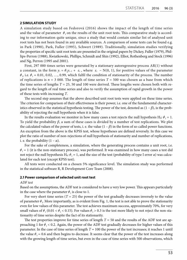
PP testThe PP test uses non-parametrically adjusted test statistics. Compared to the ADF test this fact should increase the power of tests and improve test results.

Noticeable smoothing of power functions with increasing number of replications can be seen also in this case. For time series of length T = 25 the power of the test remains very low; the results are good only for the smallest values of parameter where the power of the test for < 0.2 is above 80%. For T = 50 the test reaches almost 1 in the case of values < 0.4 and then decreases rapidly. If the time series is of length T = 100, the power of the test is significantly higher. Namely, it reaches the maximum value for < 0.7 and only after this value the power begins to decline. The test becomes very reliable in the case of lengths T = 500. Nevertheless, similarly as for the ADF test, the power of the test rapidly declines for values of close to 1.

The sizes of the test α (Figure 10) are 3.8% for T = 25, 5.8% for T = 50, 6.6% for T = 100 and 6.4% for the length of time series T = 500. For the length T = 25, this test is a conservative test as the size of the test α is notably lower than set 5% significance level, what might result in a smaller power of test. On the contrary, if time series is longer, this test is liberal as the sizes of the test are higher than the given 5% significance level up to 1.6 percentage points.

Figure 1 Power functions (1 – β) of ADF test for simulated time series of lengths T = 25, 50, 100, 500 and number of replications n = 3 000, α = 0.05

Source: Authors‘ calculation

T=25T=50T=100T=500

0.0

0.1

0.2

0.3

0.4

0.5

0.6

0.7

0.8

0.9

1.0

0.0 0.1 0.2 0.3 0.4 0.5 0.6 0.7 0.8 0.9 1.0

1 −β

φParameter 1

2016

55

96 (3)STATISTIKA

ADF-GLS testThe power functions of the ADF-GLS test, also called “efficient unit root test“, are shown in Figure 3.

The ADF-GLS test shows a noticeable increase in power with a raising number of observations as well. The shape of the power functions is, however, different at first glance; in comparison with the previous tests it is very low for small T and . For T = 25 the power is below the 40% threshold, therefore, this test is not sufficient. Even though, also in this case the power of test increases with the growing length of the time series, for T = 50 it does not reach even the 70% threshold and with the increasing value of the parameter it slowly drops. In the case of lengths T = 100 the power of the test fluctuates around 80% for 0.01 < < 0.7, then it begins to fall again. For the time series of length T = 500, we can observe greater ability to reject the null hypothesis of the unit root also for higher values of the parameter . The power of the test is approaching 1 even for the values around = 0.9. It, however, declines sharply after this value.

The sizes of the test α (Figure 10) are 10.0% for T = 25, 8.9% for T = 50, 6.9% for T = 100 and 5.9% for the length of time series T = 500. In this case, the type I errors exceed 5% significance level for any length of time series. This test is liberal for all analysed lengths of time series. For short time series, the difference reaches up to 5 p.p., it declines for longer time series. In the case of very long time series, with more than 500 observations, we can assume that the size of the test will be approaching the given 5% significance level.

NGP testThe NGP test is assumed to have high power in the case of close to 1.

As before, the power of the test is very low for T = 25, for < 0.3 it reaches only about 30% and slowly decreases. For T = 50 it fluctuates above 50% until = 0.6 and then decreases after this point. In the case

Figure 2 Power functions (1 – β) of PP test for simulated time series of lengths T = 25, 50, 100, 500 and number of replications n = 3 000, α = 0.05

Source: Authors‘ calculation

T=25T=50T=100T=500

0.0

0.1

0.2

0.3

0.4

0.5

0.6

0.7

0.8

0.9

1.0

0.0 0.1 0.2 0.3 0.4 0.5 0.6 0.7 0.8 0.9 1.0

1 −β

φParameter 1

AnAlyses

56

Figure 3 Power functions (1 – β) of ADF-GLS test for simulated time series of lengths T = 25, 50, 100, 500 and number of replications n = 3 000, α = 0.05

Source: Authors‘ calculation

T=25T=100

T=50T=500

0.0

0.1

0.2

0.3

0.4

0.5

0.6

0.7

0.8

0.9

1.0

0.0 0.1 0.2 0.3 0.4 0.5 0.6 0.7 0.8 0.9 1.0

1 −β

φParameter 1

Figure 4 Power functions (1 – β) of NGP test for simulated time series of lengths T = 25, 50, 100, 500 and number of replications n = 3 000, α = 0.05

Source: Authors‘ calculation

T=25T=100

T=50T=500

0.0

0.1

0.2

0.3

0.4

0.5

0.6

0.7

0.8

0.9

1.0

0.0 0.1 0.2 0.3 0.4 0.5 0.6 0.7 0.8 0.9 1.0

1 −β

φParameter 1

2016

57

96 (3)STATISTIKA

of lengths T = 100, the power of the test oscillates around 80% and declines from the value of parameter = 0.8. In the case of T = 500, the power reaches 1 for < 0.95 and falls sharply just before close to 1.

The sizes of the test α (Figure 10) are 4.0% for T = 25, 3.4% for T = 50, 3.2% for T = 100 and 4.6% for the length of time series T = 500. The sizes of the test are for all lengths below the 5% significance level and the test is sufficiently valid. This test is conservative for the lengths T = 25, 50 and 100 as the sizes of the test α are notably lower than given 5% significance level, by up to 1.8 p.p., in the case of long time series T = 500 is the size of test approaching the 5% significance level.

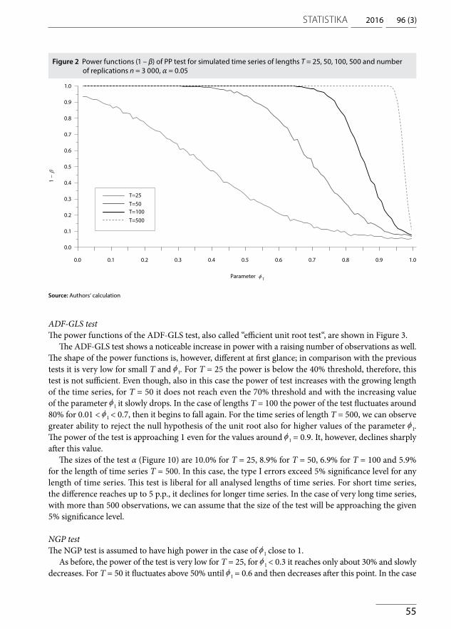
KPSS testKPSS test, unlike the other tests mentioned above, is not a unit root test, but a test of stationarity of the time series. Therefore, instead of the power functions, Figure 5 shows the probability (1 – α), i. e. the probability of not rejecting the null hypothesis when it is true.

For the values of the parameter < 0.2 the results of the KPSS test for individual lengths are very similar and the probability (1 – α) fluctuates around the selected 95% (see the line at 0.95 level in the graph). For higher values of the parameter the envelopes rapidly decline.

Interesting fact to note is that for T = 25 the probability (1 – α) is higher than this probability for T = 50 and for the value = 0.8 and bigger values it is higher than for T = 100. For > 0.9 and for shorter time series the probability (1 – α) becomes higher than in the case of longer time series.

The KPSS test is therefore considered as a suitable complement for unit root tests not only due the fact that it directly tests the stationarity, but especially because it can be used for shorter time series.

Figure 5 Probability 1 – α of KPSS test for simulated time series of lengths T = 25, 50, 100, 500 and number of replications n = 3 000, α = 0.05

Source: Authors‘ calculation

T=25T=50T=100T=500

0.0

0.1

0.2

0.3

0.4

0.5

0.6

0.7

0.8

0.9

1.0

0.0 0.1 0.2 0.3 0.4 0.5 0.6 0.7 0.8 0.9 1.0

1 −α

φParameter 1

AnAlyses

58

2.2 comparison of selected unit root testsNow, let us compare individual tests according to their ability to determine the presence of unit root or stationarity for different lengths of time series. The results of KPSS test will not be presented, the com-parison will be made based on the findings of the previous section.

Very short time series (T = 25)At first, the tests for time series of lengths T = 25 will be compared.

It is clear from Figure 6 that the power of most of the tests appears to be very low. For < 0.5 is the order of the tests according to their power as follows – PP, ADF, the power of the other tests is very low. In the interval of 0.5 < < 0.7 the power functions intersect and for higher values of this parameter is the order of the tests as follows - ADF-GLS, NGP, ADF and PP test. In the case of stationarity tests for this length (Figure 5) and lower values of the parameter , the KPSS test achieves very good results and therefore is considered to be a suitable complement in this situation.

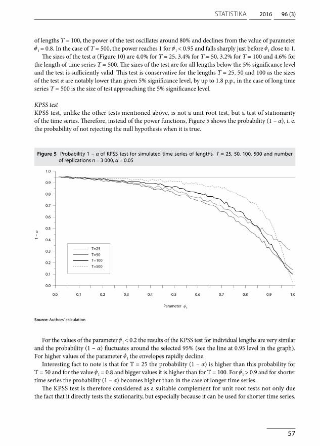
Medium-long time series (T = 50)Figure 7 shows the power of the tests for T = 50.

For this length, some of the tests reach the values close to 1. It is the case of the ADF and PP tests. The power functions of these tests are again very similar and decline rapidly from the value of parameter

= 0.4. At first, better results are achieved by the PP test, but the order changes at = 0.7 and slightly better results are observed for the ADF test.

The power of the ADF-GLS and NGP tests is again not very high for small values of the parameter . For > 0.7, however, their power reaches comparable or even better results than the other tests.

Figure 6 Comparison of power functions of selected tests for time series length T = 25, α = 0.05

Source: Authors‘ calculation

ADFPPADF-GLSNGP

0.0

0.1

0.2

0.3

0.4

0.5

0.6

0.7

0.8

0.9

1.0

0.0 0.1 0.2 0.3 0.4 0.5 0.6 0.7 0.8 0.9 1.0

1 −β

φParameter 1

2016

59

96 (3)STATISTIKA

The power functions intersect around this value and for higher values of this parameter is the order of the tests as follows – ADF-GLS, NGP, ADF and PP. The conclusion is therefore the same as for T = 25. KPSS test can be used as a complementary test also for this length.

Long time series (T = 100)The power of the tests increases with the increasing length of time series (see Figure 8).

As for the shorter lengths, also in this case the ADF and PP tests reach the best results for small values of parameter . The power of both tests equals 1 for < 0.6. Afterwards, it sharply declines. KPSS test can be also used.

The power of ADF-GLS and NGP tests is for > 0.8 even higher when compared to ADF and PP. The advantages of modifications of classic unit root tests, i. e. NGP and ADF-GLS, can already be observed.

Very long time series (T = 500)The results of all tests for time series of length T = 500 are very good and the power functions have much similar shape.

The results of the ADF and PP tests are in this case almost undistinguishable; their power reaches 100% for < 0.9 and then it suddenly and sharply declines.

The values of power of the ADF-GLS test fluctuate below the level of 100 %. In this case a steep de-cline of power function occurs already for > 0.8. The NGP test shows considerably better results than for shorter time series. It reaches 100% for < 0.95 and its power for close to 1 is still the highest in comparison with other tests.

The order of the tests according to their power for close to 1 is as follows – NGP, ADF-GLS, ADF, PP, KPSS test cannot be recommended for this length.

Figure 7 Comparison of power functions of selected tests for time series length T = 50, α = 0.05

Source: Authors‘ calculation

ADFPPADF-GLSNGP

0.0

0.1

0.2

0.3

0.4

0.5

0.6

0.7

0.8

0.9

1.0

0.0 0.1 0.2 0.3 0.4 0.5 0.6 0.7 0.8 0.9 1.0

1 −β

φParameter 1

AnAlyses

60

Figure 8 Comparison of power functions of selected tests for time series length T = 100, α = 0.05

Source: Authors‘ calculation

ADFPPADF-GLSNGP

0.0

0.1

0.2

0.3

0.4

0.5

0.6

0.7

0.8

0.9

1.0

0.0 0.1 0.2 0.3 0.4 0.5 0.6 0.7 0.8 0.9 1.0

1 −β

φParameter 1

Figure 9 Comparison of power functions of selected tests for time series length T = 500, α = 0.05

Source: Authors‘ calculation

ADFPPADF-GLSNGP

0.0

0.1

0.2

0.3

0.4

0.5

0.6

0.7

0.8

0.9

1.0

0.0 0.1 0.2 0.3 0.4 0.5 0.6 0.7 0.8 0.9 1.0

1 −β

φParameter 1

2016

61

96 (3)STATISTIKA

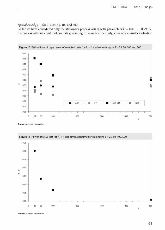
Special case = 1, for T = 25, 50, 100 and 500So far we have considered only the stationary process AR(1) with parameters = 0.01, …, 0.99, i.e. the process without a unit root, for data generating. To complete the study, let us now consider a situation

Figure 10 Estimations of type I error of selected tests for = 1 and series lengths T = 25, 50, 100 and 500

Figure 11 Power of KPSS test for = 1 and simulated time series lengths T = 25, 50, 100, 500

Source: Authors‘ calculation

Source: Authors‘ calculation

0.00

0.01

0.02

0.03

0.04

0.05

0.06

0.07

0.08

0.09

0.10

0.11

0 100 200 300 400 500 5025T

ADF PP ADF-GLS NGP

α

0.00

0.05

0.10

0.15

0.20

0.25

0.30

0.35

0 100 200 300 400 500 5025T

1 −β

AnAlyses

62

where the generating process contains a unit root, i.e. = 1, therefore we speak about a non-stationary random walk process.

Figure 10 shows the estimates of probabilities of the type I. errors of individual tests (without KPSS test) for T = 25, 50, 100 and 500. This figure shows that valid tests for the length T = 25 are PP, NGP and ADF that are below 5% of the nominal significance level, in contrary ADF-GLS test is notably above this level and therefore is not suitable for this length. For the same reason only the ADF and NGP tests can be used for lengths T = 50, 100 and 500.

To complete the results Fig. 11 has been created to show the power of KPSS test.

2.3 results summaryIt is evident that it is impossible to choose the only test that could be generally described as the best for unit root testing in time series for any length T and any value of the parameter at the same time. Table 1 shows the summary of the results of our simulation study and recommendations which tests are appropriate for given length T and value of the parameter . We have taken into consideration three basic aspects – power of the test, its validity and ease of use.

The most suitable tests for very short time series are the ADF and PP tests, the best results were ob-tained for length T = 25. KPSS test can be used for refinement in the case of lower values of parameter

. For higher values of parameter , the NGP test is also suitable.The best results for time series of lengths T = 50 were obtained by ADF test. For lower values

of parameter the PP and KPSS tests are sufficient, in contrary, NGP test can be used for > 0.7.The most appropriate test for values > 0.8 and length T = 100 was the ADF test, a suitable comple-

ment for < 0.7 is the PP test and for > 0.7, the NGP test.In the case of very long time series, i.e. in our case for T = 500, the results of all the analysed tests

were very similar. The best results for < 0.9 were achieved by the NGP, ADF and PP tests, for > 0.9 by the ADF-GLS and NGP tests.

concLuSIonUnit root testing in time series is one of the fundamental steps in the construction of univariate and multivariate econometric models. As the theory offers several possible unitroot tests, the aim of this paper was to make recommendations to analysts which test to choose based on given parameters. The results were obtained from a simulation study where the criteria were the length of time series and value of the parameter in the autoregressive process AR(1) without drift.

Table 1 was created based on the results of the simulation study and it gives clear recommendations which tests should be used based on the length of time series and the value of the parameter . The highest

Table 1 Overview of appropriate tests for different lengths of time series and values of parameter , α = 0.05

T

25 50 100 500

(0; 0.5> PP, ADF, + KPSS PP, ADF, + KPSS ADF, PP ADF, PP, NGP

(0.5; 0.7> PP, ADF, + KPSS PP, ADF, + KPSS ADF, PP ADF, PP, NGP

(0.7; 0.9> ADF, NGP, PP ADF, NGP, PP ADF, NGP ADF, NGP

(0.9; 1> PP, NGP, ADF ADF, NGP ADF, NGP ADF, NGP

Source: Authors‘ calculation

2016

63

96 (3)STATISTIKA

power for shorter time series was achieved the ADF and PP tests. KPSS test, which tests the stationarity is suitable for very small values of the parameter , we do not recommended to use it independently, but only as complementary test during the unit root testing of shorter time series. The ability of other tests to reject the null hypothesis of the unit root increased with the increasing length of time series. Signifi-cantly better results were achieved by the ADF and PP tests especially for lower values of the parameter

. Very good results for higher values of this parameter were achieved by the modified NGP test.The results show that the ADF test is a reliable option for unit root testing, its results are very good

especially in the case of time series with bigger number of observations. PP test is a suitable substitute for very short time series, or another recommendation could be a simultaneous use of KPSS test. How-ever, despite this lack, the ADF test is and will be one of the most commonly used unit root test since its crucial advantage lies in its simple construction and feasibility.

Despite the fact that our simulation study is relatively rare, we do realize its rather narrow focus (re-sulting from the use of the autoregressive process AR(1), with positive values of the parameter only) and the possibility to extend it quite significantly in the future. This extension would be possible not only for the negative values of the parameter , but also for autoregressive processes with deterministic components (constant and linear trend), for autoregressive processes of higher order, for processes that contain a combination of autoregressive process and process of moving averages, for different significance levels α and even for longer time series.

AcKnoWLEdGEMEntSThis paper was written with the support of the Czech Science Foundation project No. P402/12/G097 DYME – Dynamic Models in Economics.

References

BOX, G. E. P, JENKINS, G. M. Time Series Analysis, Forecasting and Control. San Francisco: Holden-Day, 1970.CANER, M., KILIAN, L. Size Distortions of Tests of the Null Hypothesis of Stationarity: Evidence and Implications

for the PPP Debate. Journal of International Money and Finance, 2001, Vol. 20, pp. 639–657. DICKEY, D. A. Estimation and Hypothesis Testing in Nonstationary Time Series. Iowa State University Ph.D. Thesis, 1976.DICKEY, D. A., FULLER, W. A. Distribution of the Estimators for Autoregressive Time Series with a Unit Root. Journal

of the American Stat. Association, 1979, 74, pp. 427–431.DICKEY, D. A., FULLER, W. A. Likelihood Ratio Statistics for Autoregressive Time Series with a Unit Root. Econometrica,

1981, 49, pp. 1057–72.ELDER, J., KENNEDY, P. E. Testing for Unit Roots: What Should Students Be Taught? Journal of Economic Education,

2001, Vol. 32, No. 2, pp. 137–146. DOI: 10.2307/1183489. ELLIOT, G., ROTHENBERG, T. J., STOCK, J. H. Efficient Tests for an Autoregressive Unit Root. Econometrica, 1996,

Vol. 64, No. 4, pp. 813–836. ENDERS, W. Applied Econometric Time Series. 2nd Ed. Hoboken: Wiley, 2004. FEDOROVÁ, D. Vybrané testy jednotkových kořenů v časových řadách. Diploma thesis, Prague: VŠE, 2016.FULLER, W. A. Introduction to Statistical Time Series. New York: John Wiley & Sons, 1976.KWIATKOWSKI, D., PHILLIPS, P. C. B., SCHMIDT, P. SHIN, Y. Testing the Null Hypothesis of Stationarity Against

the Alternative of a Unit Root. Journal of Econometrics, 1992, 54, pp. 159–178. DOI: 10.1016/0304-4076(92)90104-Y.MACKINNON, J. G. Critical Values for Cointegration Tests. In: ENGLE, R. F., GRANGER, C. W. J., eds. Long Run Economic

Relationships. Oxford University Press, 1991, pp. 267–276.NG, S., PERRON, P. Lag Length Selection and the Construction of Unit Root Tests with Good Size and Power. Econometrica,

November 2001, Vol. 69, No. 6, pp. 1519–1554. NG, S., PERRON, P. Unit Root Tests in ARMA Models with Data-Dependent Methods for the Selection of the Truncation

Lag. Journal of the American Statistical Association, March 1995, Vol. 90, No. 429, pp. 268–281. PARK, H. J. Alternative Estimators of the Parameters of the Autoregressive Process. Retrospective Theses and Dissertations,

Paper 9880, Iowa State University, 1990.

AnAlyses

64

PARK, H. J., FULLER, W. A. Alternative Estimators and Unit Root Tests for the Autoregressive Process. Journal Time Series Analysis, 1995, 16, pp. 415–429.

PESARAN, M. H. Time Series and Panel Data Econometrics. Oxford University Press, 2015.PHILLIPS, P. C. B. Time Series Regression with a Unit Root. Econometrica, Vol. 55, 1987, No. 2, pp. 277–301. PHILLIPS, P. C. B., PERRON, P. Testing for a unit root in a time series regression. Biometrika, 1988, Vol. 75, No. 2, pp. 335–346.R DEVELOPMENT CORE TEAM. R: A Language and Environment for Statistical Computing [online]. R Foundation

for Statistical Computing, Vienna, Austria, 2008. <http://www.R-project.org>.SCHWERT, G. W. Test for Unit Roots: A Monte Carlo Investigation. Journal of Business & Economic Statistics, 1989,

Vol. 7, No. 2, pp. 147–159.ZIVOT, E. Unit root tests [online]. 2006. <http://faculty.washington.edu/ezivot/econ584/notes/unitroot.pdf>.