Page 1
293
Standard Costing
Practical Question on Standard Costing Question 1: The standard cost of a certain chemical mixture is as under:
40% of Material A @ `30 per kg
60% of Material B @ `40 per kg
A standard loss of 10% of input is expected in production. The following actual cost data
is given for the period.
350 kg Material – A at a cost of `25
400 kg Material – B at a cost of `45
Actual weight produced is 620 kg.
You are required to calculate the following variances raw material wise and indicate
whether they are favorable (F) or adverse (A):
(i) Cost variance
(ii) Price variance
(iii) Mix variance
(iv) Yield variance Solution:
Actual Output produced is 630 Kg. The Standard Quantity of Material required for 630 Kg. of output is
700 Kg.
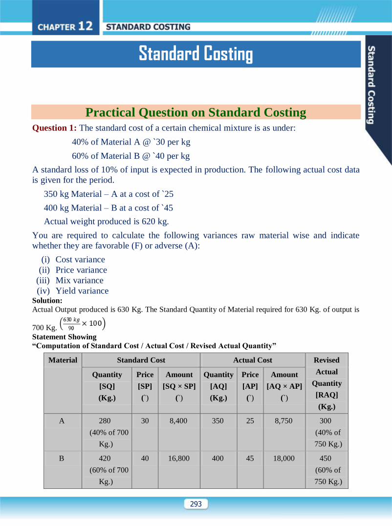
Statement Showing
“Computation of Standard Cost / Actual Cost / Revised Actual Quantity”
Material Standard Cost Actual Cost Revised
Actual
Quantity
[RAQ]
(Kg.)
Quantity
[SQ]
(Kg.)
Price
[SP]
(`)
Amount
[SQ × SP]
(`)
Quantity
[AQ]
(Kg.)
Price
[AP]
(`)
Amount
[AQ × AP]
(`)
A 280
(40% of 700
Kg.)
30 8,400 350 25 8,750 300
(40% of
750 Kg.)
B 420
(60% of 700
Kg.)
40 16,800 400 45 18,000 450
(60% of
750 Kg.)
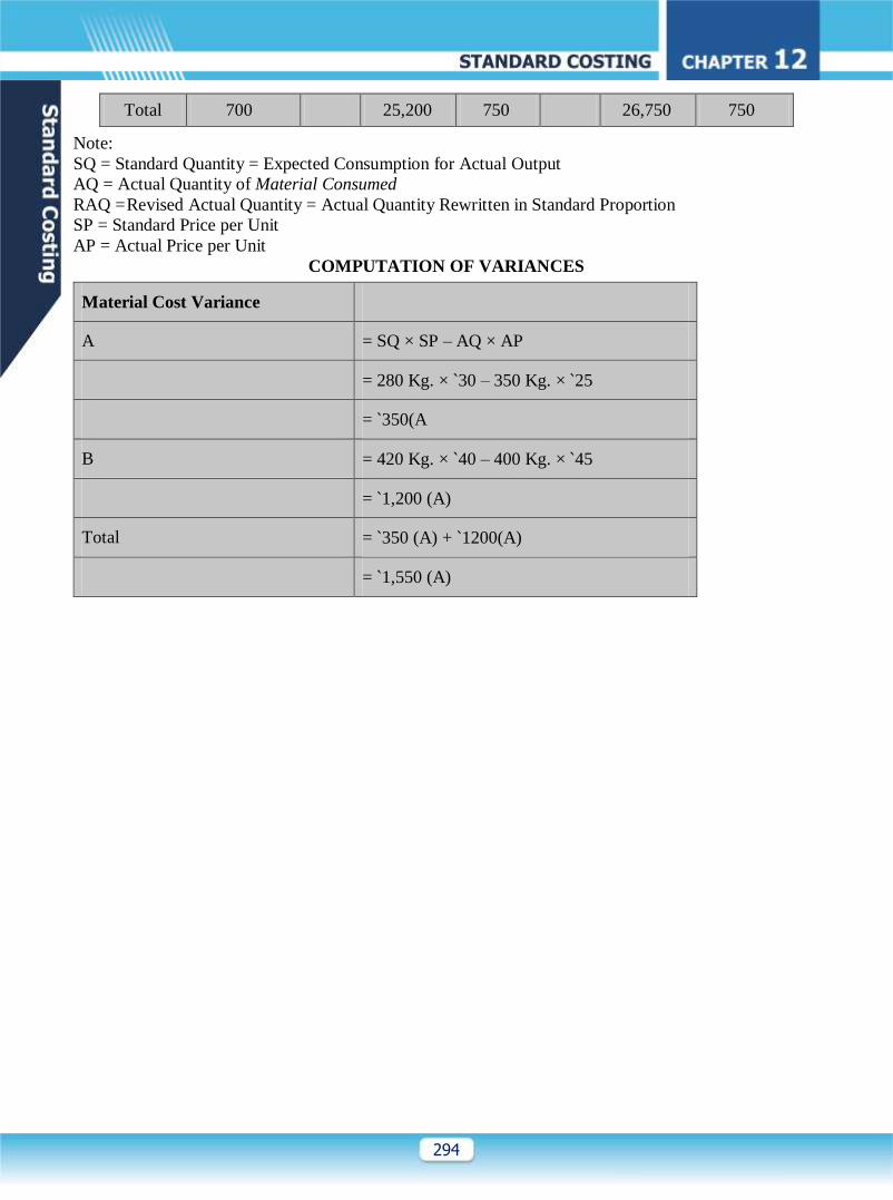
Page 2
294
Total 700 25,200 750 26,750 750
Note:
SQ = Standard Quantity = Expected Consumption for Actual Output
AQ = Actual Quantity of Material Consumed
RAQ = Revised Actual Quantity = Actual Quantity Rewritten in Standard Proportion
SP = Standard Price per Unit
AP = Actual Price per Unit
COMPUTATION OF VARIANCES
Material Cost Variance
A = SQ × SP – AQ × AP
= 280 Kg. × `30 – 350 Kg. × `25
= `350(A
B = 420 Kg. × `40 – 400 Kg. × `45
= `1,200 (A)
Total = `350 (A) + `1200(A)
= `1,550 (A)
Page 3
295
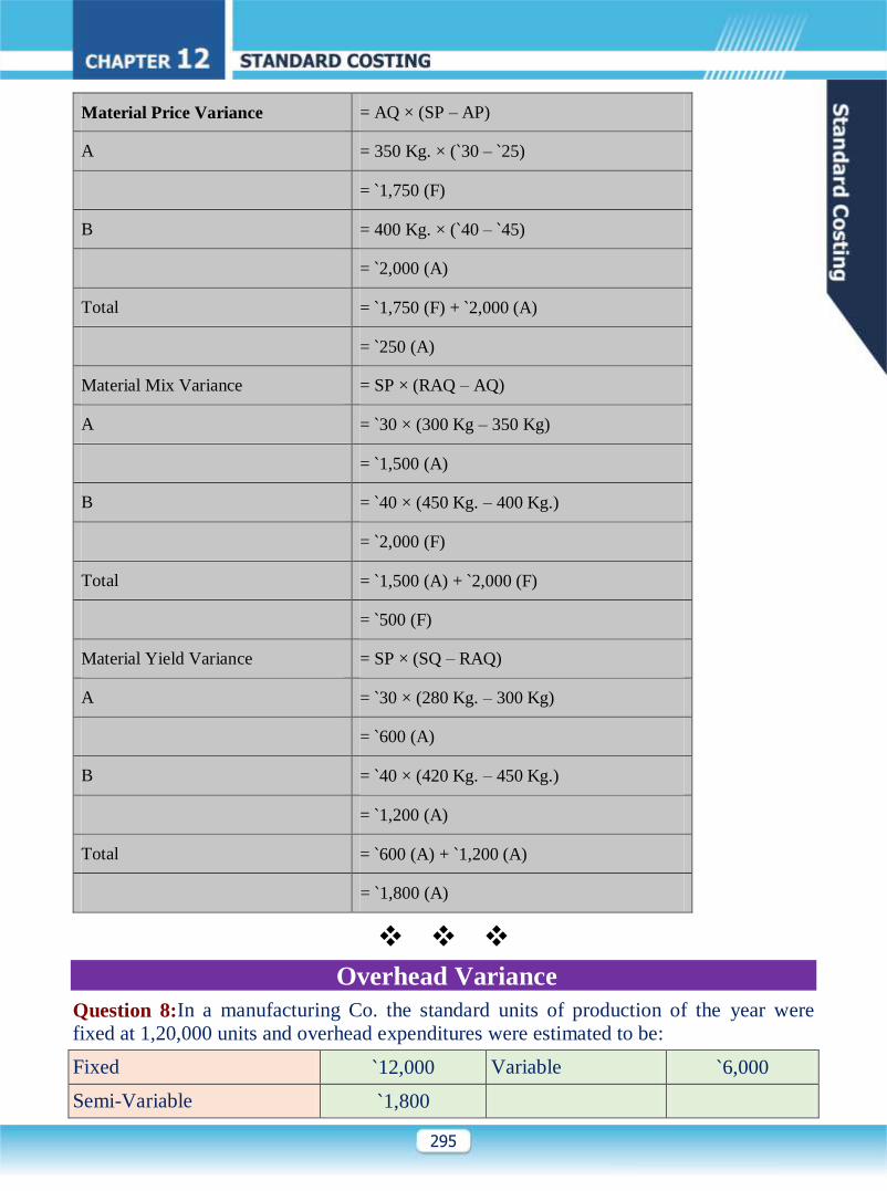
Material Price Variance = AQ × (SP – AP)
A = 350 Kg. × (`30 – `25)
= `1,750 (F)
B = 400 Kg. × (`40 – `45)
= `2,000 (A)
Total = `1,750 (F) + `2,000 (A)
= `250 (A)
Material Mix Variance = SP × (RAQ – AQ)
A = `30 × (300 Kg – 350 Kg)
= `1,500 (A)
B = `40 × (450 Kg. – 400 Kg.)
= `2,000 (F)
Total = `1,500 (A) + `2,000 (F)
= `500 (F)
Material Yield Variance = SP × (SQ – RAQ)
A = `30 × (280 Kg. – 300 Kg)
= `600 (A)
B = `40 × (420 Kg. – 450 Kg.)
= `1,200 (A)
Total = `600 (A) + `1,200 (A)
= `1,800 (A)
Overhead Variance
Question 8:In a manufacturing Co. the standard units of production of the year were
fixed at 1,20,000 units and overhead expenditures were estimated to be:
Fixed `12,000 Variable `6,000
Semi-Variable `1,800
Page 4
296
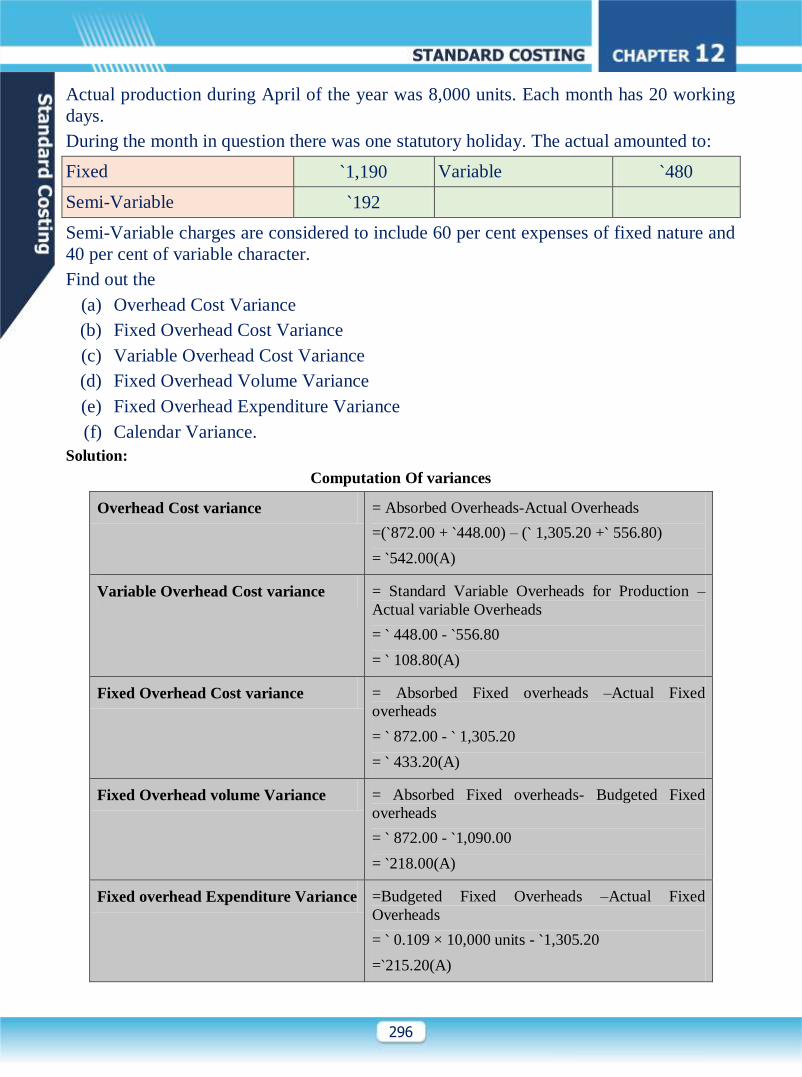
Actual production during April of the year was 8,000 units. Each month has 20 working
days.
During the month in question there was one statutory holiday. The actual amounted to:
Fixed `1,190 Variable `480
Semi-Variable `192
Semi-Variable charges are considered to include 60 per cent expenses of fixed nature and
40 per cent of variable character.
Find out the
(a) Overhead Cost Variance
(b) Fixed Overhead Cost Variance
(c) Variable Overhead Cost Variance
(d) Fixed Overhead Volume Variance
(e) Fixed Overhead Expenditure Variance
(f) Calendar Variance.
Solution:
Computation Of variances
Overhead Cost variance = Absorbed Overheads-Actual Overheads
=(`872.00 + `448.00) – (` 1,305.20 +` 556.80)
= `542.00(A)
Variable Overhead Cost variance = Standard Variable Overheads for Production –
Actual variable Overheads
= ` 448.00 - `556.80
= ` 108.80(A)
Fixed Overhead Cost variance = Absorbed Fixed overheads –Actual Fixed
overheads
= ` 872.00 - ` 1,305.20
= ` 433.20(A)
Fixed Overhead volume Variance = Absorbed Fixed overheads- Budgeted Fixed
overheads
= ` 872.00 - `1,090.00
= `218.00(A)
Fixed overhead Expenditure Variance =Budgeted Fixed Overheads –Actual Fixed
Overheads
= ` 0.109 × 10,000 units - `1,305.20
=`215.20(A)
Page 5
297
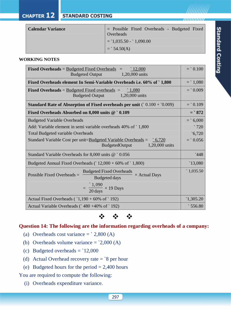
Calendar Variance = Possible Fixed Overheads - Budgeted Fixed
Overheads
= `1,035.50 - ` 1,090.00
= ` 54.50(A)
WORKING NOTES
Fixed Overheads = Budgeted Fixed Overheads = ` 12,000
Budgeted Output 1,20,000 units
= ` 0.100
Fixed Overheads element In Semi-Variable Overheads i.e. 60% of ` 1,800 = ` 1,080
Fixed Overheads = Budgeted Fixed overheads = ` 1,080
Budgeted Output 1,20,000 units
= ` 0.009
Standard Rate of Absorption of Fixed overheads per unit (` 0.100 + `0.009) = ` 0.109
Fixed Overheads Absorbed on 8,000 units @ ` 0.109 = ` 872
Budgeted Variable Overheads
Add: Variable element in semi variable overheads 40% of ` 1,800
Total Budgeted variable Overheads
Standard Variable Cost per unit=Budgeted Variable Overheads = ` 6,720
BudgetedOutput 1,20,000 units
= ` 6,000
` 720
`6,720
= ` 0.056
Standard Variable Overheads for 8,000 units @ ` 0.056 `448
Budgeted Annual Fixed Overheads (` 12,000 + 60% of ` 1,800) `13,080
Possible Fixed Overheads = Budgeted Fixed Overheads
Budgeted days × Actual Days
= 1,090
20 days
` × 19 Days
` 1,035.50
Actual Fixed Overheads ( `1,190 + 60% of ` 192) `1,305.20
Actual Variable Overheads (` 480 +40% of ` 192) ` 556.80
Question 14: The following are the information regarding overheads of a company:
(a) Overheads cost variance = ` 2,800 (A)
(b) Overheads volume variance = `2,000 (A)
(c) Budgeted overheads = `12,000
(d) Actual Overhead recovery rate = `8 per hour
(e) Budgeted hours for the period = 2,400 hours
You are required to compute the following:
(i) Overheads expenditure variance.
Page 6
298
(ii) Actual incurred overheads.
(iii) Actual hours for actual production.
(iv) Overheads capacity variance.
(v) Overheads efficiency variance.
(vi) Standard hours for actual production.
Solution:
BASIC WORKINGS
Overheads Cost Variance = ` 2,800 (A)
Overheads Volume Variance = ` 2,000 (A)
Budgeted Overheads = ` 12,000
Actual Overhead Recovery Rate = ` 8 per hour
Budgeted Hours for the period = 2,400 hours
COMPUTATION OF REQUIREMENTS
Overheads expenditure variance
Overheads Expenditure Variance = Overheads Cost Variance (–) Overheads Volume Variance
= ` 2,800 (A) – ` 2,000 (A)
= ` 800 (A)
Actual incurred overheads
Overheads Expenditure Variance = Budgeted Overheads (–) Actual Overheads
` 800(A) = ` 12,000 (–) Actual Overheads
Therefore, Actual Overheads = ` 12,800
Actual hours for actual production
Actual hours for actual production =
=
= 1,600 hours
Overheads capacity variance
Overheads Capacity Variance = Budgeted Overheads for Actual Hours (–) Budgeted Overheads
= ` 5 × 1,600 hrs. – ` 12,000
= ` 8,000 – ` 12,000
= ` 4,000 (A)
Overheads efficiency variance
Overheads Efficiency Variance = Absorbed Overheads (–) Budgeted Overheads for Actual Hours
Page 7
299
= ` 10,000 – ` 5 × 1,600 hours
= ` 2,000 (F)
Standard hours for actual production
Standard hours for actual output =
=
= 2,000 hours
WORKING NOTE
Overhead Cost Variance = Absorbed Overheads (–) Actual Overheads
` 2,800 (A) = Absorbed Overheads (–) `12,800
Absorbed Overheads = `10,000
Standard Rate per hour =
=
= ` 5
Question 16:The Standard Cost Sheet per unit for the product produced by Style
Manufactures is worked out on this basis:—
Direct Materials 1.3 tons @`4.00 per ton
Direct Labour 2.9 hours @ `2.30 per hour
Factory Overhead 2.9 hours @ `2.00 per hour
Normal Capacity is 2,00,000 direct labour hours per month.
The Factory Overhead rate is arrived at on the basis of a fixed Overhead of `1,00,000 per
month and a Variable Overhead of `1.50 per direct labour hour.
In the month of May, 50,000 units of the product was started and completed. An
investigation of the raw material inventory account reveals that 78,000 tons of raw
materials were transferred into and used by the factory during May. These goods cost
`4.20 per ton. 1,50,000 hours of Direct Labour were spent during May at a cost of `2.50
per hour. Factory Overhead for the month amounted to `3, 40,000 out of which `1, 02,000
was fixed.
Compute and identify all variances under Material, Labour and overhead as favourable or
adverse.
Identify one or more departments in the company who might be held responsible for each
variance.
Page 8
300
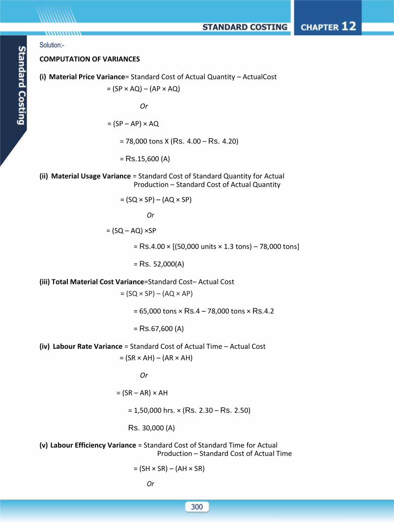
Solution:-
COMPUTATION OF VARIANCES
(i) Material Price Variance= Standard Cost of Actual Quantity – ActualCost
= (SP × AQ) – (AP × AQ)
Or
= (SP – AP) × AQ
= 78,000 tons X (Rs. 4.00 – Rs. 4.20)
= Rs.15,600 (A)
(ii) Material Usage Variance = Standard Cost of Standard Quantity for Actual Production – Standard Cost of Actual Quantity
= (SQ × SP) – (AQ × SP)
Or
= (SQ – AQ) ×SP
= Rs.4.00 × [(50,000 units × 1.3 tons) – 78,000 tons]
= Rs. 52,000(A)
(iii) Total Material Cost Variance=Standard Cost– Actual Cost
= (SQ × SP) – (AQ × AP)
= 65,000 tons × Rs.4 – 78,000 tons × Rs.4.2
= Rs.67,600 (A)
(iv) Labour Rate Variance = Standard Cost of Actual Time – Actual Cost
= (SR × AH) – (AR × AH)
Or
= (SR – AR) × AH
= 1,50,000 hrs. × (Rs. 2.30 – Rs. 2.50)
Rs. 30,000 (A)
(v) Labour Efficiency Variance = Standard Cost of Standard Time for Actual Production – Standard Cost of Actual Time
= (SH × SR) – (AH × SR)
Or
Page 9
301
= (SH – AH) ×SR
= Rs.2.30 × [(50,000 units × 2.9 hrs.) – 1,50,000 hrs.]
= Rs.11,500 (A
(vi) Total Labour Cost Variance= Standard Cost – Actual Cost
= (SH × SR) – (AH × AR)
= (1,45,000 hrs. × Rs.2.30) – (1,50,000 hrs. × Rs.2.50)
= Rs.41,500 (A)
(vii) Variable Overhead Cost = Standard Variable Overheads for Production– Variance Actual Variable Overheads
= (50,000 units × 2.9 hrs. × Rs.1.50) – Rs.2,38,000
= Rs.20,500 (A)
(viii) Fixed Overhead Expenditure = Budgeted Fixed Overheads – Actual Fixed Overheads Variance = Rs.1,00,000 – Rs.1,02,000
= Rs. 2,000 (A)
(ix) Fixed Overhead Volume = Absorbed Fixed Overheads – Budgeted Fixed Overheads Variance = 2.9 hrs. × Rs.0.50 × 50,000 units –Rs.1,00,000
= Rs. 27,500 (A)
(x) Fixed Overhead Capacity = Budgeted Fixed Overheads for Actual Hours –
Budgeted Fixed Variance Overheads
= (1,50,000 hrs. × Rs.0.50) – Rs.1,00,000
= Rs. 25,000 (A)
(xi) Fixed Efficiency Variance= Absorbed Fixed Overheads – Budgeted Fixed Overheads for Actual
Hours
= (2.9 hrs. × Rs.0.50 × 50,000 units) – (1,50,000 hrs.× Rs.0.50)
= Rs. 2,500 (A)
(xii) Total Fixed Overhead Variance = Absorbed Fixed Overheads – Actual Fixed Overheads
= (2.9 hrs. × Rs.0.50 × 50,000 units) – Rs.1,02,000
= Rs. 29,500 (A)
IDENTIFICATION OF DEPARTMENT(S) WHO MIGHT BE HELD RESPONSIBLE FOR EACH VARIANCE
Page 10
302
Name of Variance Name of the Department
Material Price Variance .................................. Purchase Department
Material Usage Variance ............................... Production Department / Factory Foreman
Labour Rate Variance .................................... Personnel Department / Manager Policy
Labour Efficiency Variance ............................. Production Department / Factory Foreman
Overhead Variances .......................................Production Department / Factory Foreman
Question 18:Bajaj Ltd. produces a product “M”. The following information is
available:
For one unit of product the standard materials input is 20 meters at a standard price of ` 2
per meter. The standard wage rate is ` 6 per hour and 5 hours are allowed in which to
produce one unit.
Fixed production overhead is absorbed at the rate of 100% of direct wages cost. During
the month just ended the following occurred:
Actual price paid for material purchased ` 1.95 per meter
Total direct wages cost was ` 1,56,000
Fixed production overhead incurred was ` 1,58,000
Variances Favorable (`) Adverse (`)
Direct material price (at the time of purchase) 8,000 -
Direct material usage - 5,000
Direct labour rate - 5,760
Direct labour efficiency 2,760 -
Fixed production overhead expenditure - 8,000
Required:
Calculate the following for the month:
• Actual units produced.
• Actual hours worked
• Budgeted output in units,
• Number of meter purchased,
• Number of meters used above standard allowed.
• Average actual wage rate per hour.
Answer:
Page 11
303
Budgeted output in units
Fixed Overhead Expenditure = Budgeted Fixed Overheads –Actual Fixed Overheads Variance
= Rs.8,000 (A) = Budgeted output X ( Rs.6 X 5 hrs.) - Rs. 1,58,000
Budgeted output = 5,000 units
Number of liters purchased
Material Price variance = Actual Quantity X (Std Price –Actual Price)
=Rs.8,000 (F) = No. of liters purchased X (Rs.2 - Rs.1.95)
= No. of liters purchased = 1,60,000 liters
Number of liters used above standard allowed
Material Usage Variance = Standard Price X (Standard Quantity – Actual Quantity)
= Rs.5000 (A) = Rs.2 X ( standard Quantity – 1,60,000 liters)
= standard Quantity = 1,57,500 liters
No. of liters above Standard = 1,60,000 liters – 1,57,500 liters
= 2,500 liters
Actual units produced
Labour Cost Variance =Rate Variance + Efficiency Variance
= Rs.5,760 (A) + Rs. 2,760 (F)
= Rs.3,000 (A)
Labour Cost Variance =Standard Cost- Actual Cost
=Rs.3000 (A) = Actual Output X (Rs.6 X 5 hrs) - Rs.1,56,000
= Actual output = 5,100 units
Actual hours worked
Page 12
304
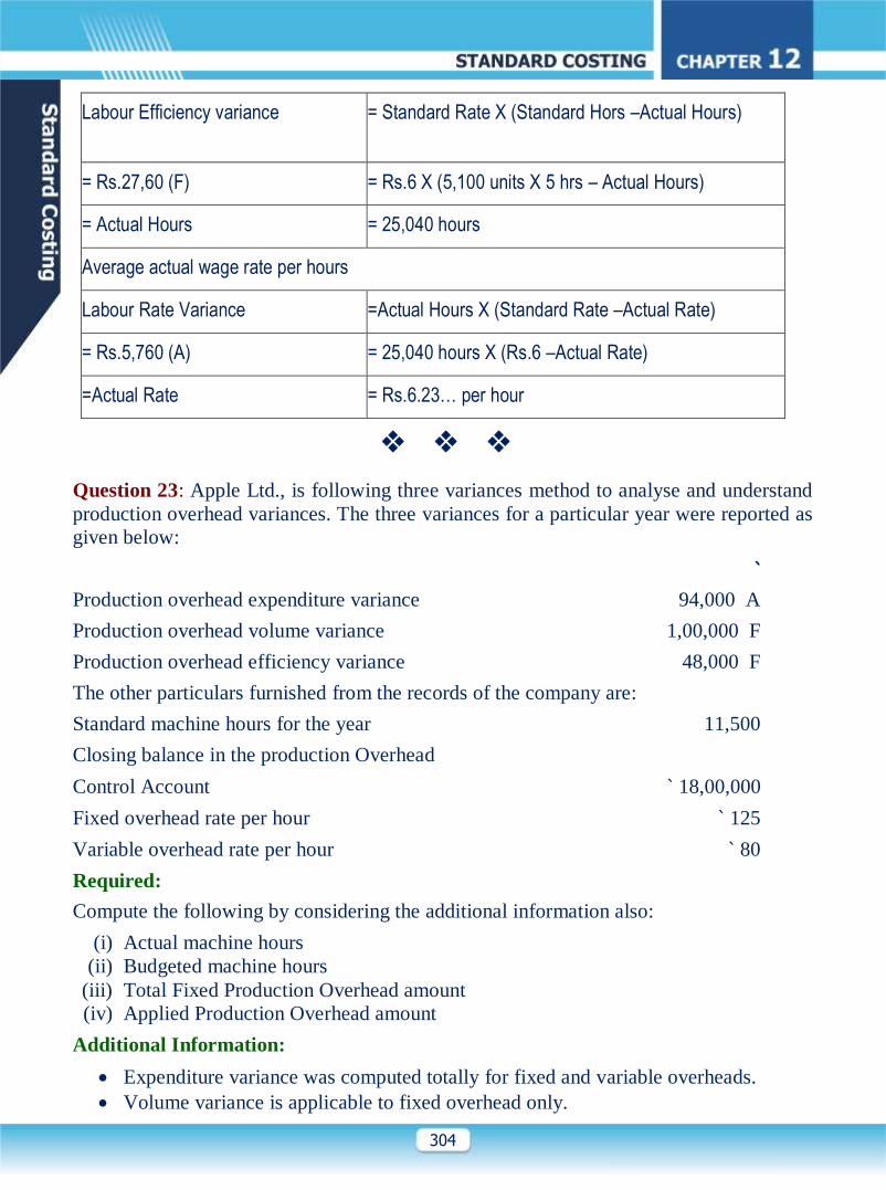
Labour Efficiency variance = Standard Rate X (Standard Hors –Actual Hours)
= Rs.27,60 (F) = Rs.6 X (5,100 units X 5 hrs – Actual Hours)
= Actual Hours = 25,040 hours
Average actual wage rate per hours
Labour Rate Variance =Actual Hours X (Standard Rate –Actual Rate)
= Rs.5,760 (A) = 25,040 hours X (Rs.6 –Actual Rate)
=Actual Rate = Rs.6.23… per hour
Question 23: Apple Ltd., is following three variances method to analyse and understand
production overhead variances. The three variances for a particular year were reported as
given below:
`
Production overhead expenditure variance 94,000 A
Production overhead volume variance 1,00,000 F
Production overhead efficiency variance 48,000 F
The other particulars furnished from the records of the company are:
Standard machine hours for the year 11,500
Closing balance in the production Overhead
Control Account ` 18,00,000
Fixed overhead rate per hour ` 125
Variable overhead rate per hour ` 80
Required:
Compute the following by considering the additional information also:
(i) Actual machine hours
(ii) Budgeted machine hours
(iii) Total Fixed Production Overhead amount
(iv) Applied Production Overhead amount
Additional Information:
Expenditure variance was computed totally for fixed and variable overheads.
Volume variance is applicable to fixed overhead only.
Page 13
305
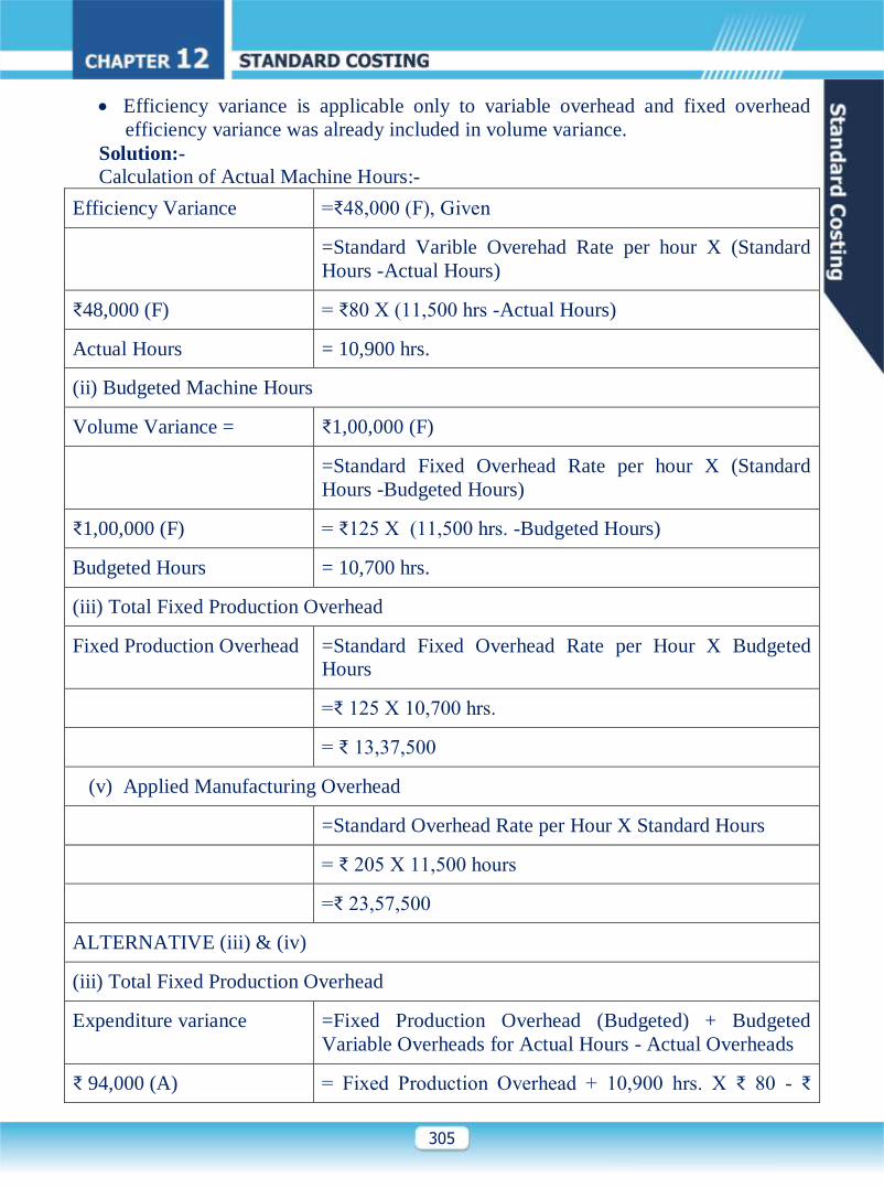
Efficiency variance is applicable only to variable overhead and fixed overhead
efficiency variance was already included in volume variance.
Solution:-
Calculation of Actual Machine Hours:-
Efficiency Variance =₹48,000 (F), Given
=Standard Varible Overehad Rate per hour X (Standard
Hours -Actual Hours)
₹48,000 (F) = ₹80 X (11,500 hrs -Actual Hours)
Actual Hours = 10,900 hrs.
(ii) Budgeted Machine Hours
Volume Variance = ₹1,00,000 (F)
=Standard Fixed Overhead Rate per hour X (Standard
Hours -Budgeted Hours)
₹1,00,000 (F) = ₹125 X (11,500 hrs. -Budgeted Hours)
Budgeted Hours = 10,700 hrs.
(iii) Total Fixed Production Overhead
Fixed Production Overhead =Standard Fixed Overhead Rate per Hour X Budgeted
Hours
=₹ 125 X 10,700 hrs.
= ₹ 13,37,500
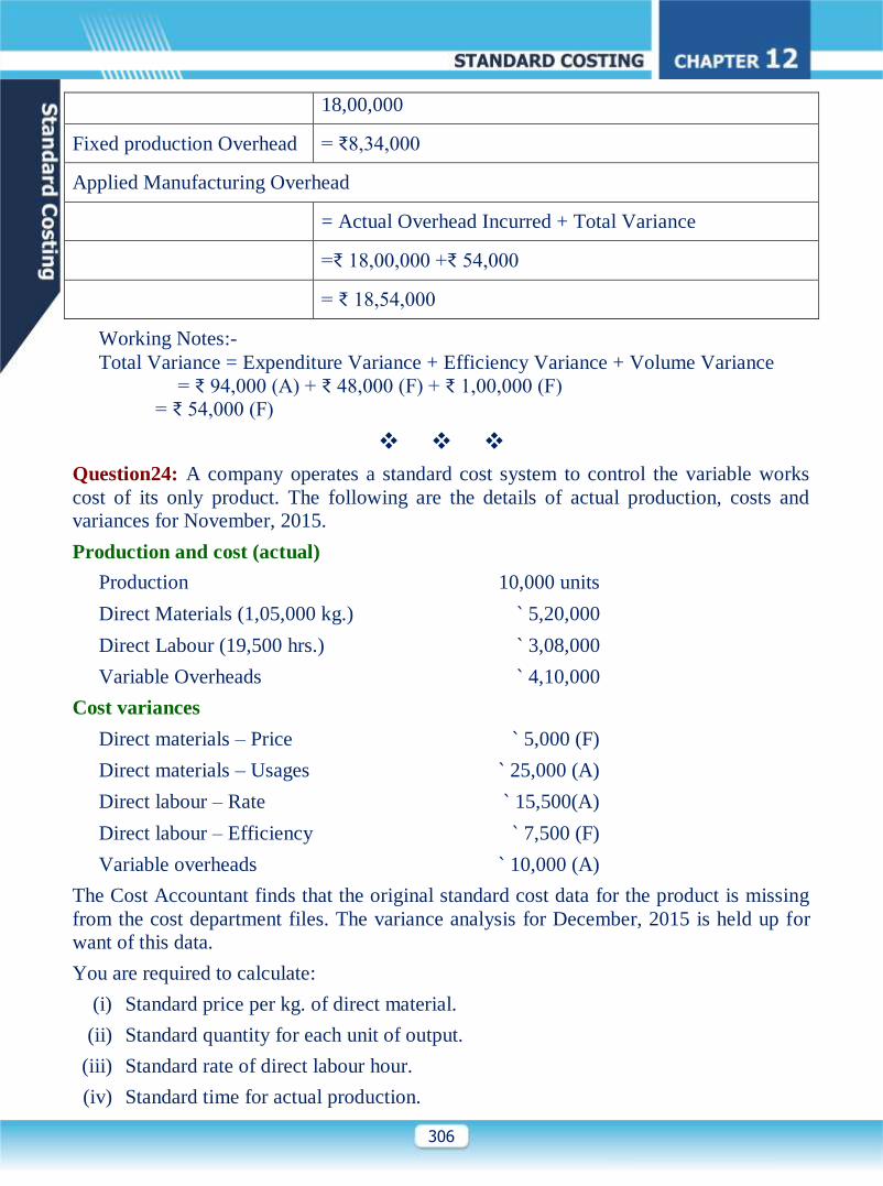
(v) Applied Manufacturing Overhead
=Standard Overhead Rate per Hour X Standard Hours
= ₹ 205 X 11,500 hours
=₹ 23,57,500
ALTERNATIVE (iii) & (iv)
(iii) Total Fixed Production Overhead
Expenditure variance =Fixed Production Overhead (Budgeted) + Budgeted
Variable Overheads for Actual Hours - Actual Overheads
₹ 94,000 (A) = Fixed Production Overhead + 10,900 hrs. X ₹ 80 - ₹
Page 14
306
18,00,000
Fixed production Overhead = ₹8,34,000
Applied Manufacturing Overhead
= Actual Overhead Incurred + Total Variance
=₹ 18,00,000 +₹ 54,000
= ₹ 18,54,000
Working Notes:-
Total Variance = Expenditure Variance + Efficiency Variance + Volume Variance
= ₹ 94,000 (A) + ₹ 48,000 (F) + ₹ 1,00,000 (F)
= ₹ 54,000 (F)
Question24: A company operates a standard cost system to control the variable works
cost of its only product. The following are the details of actual production, costs and
variances for November, 2015.
Production and cost (actual)
Production 10,000 units
Direct Materials (1,05,000 kg.) ` 5,20,000
Direct Labour (19,500 hrs.) ` 3,08,000
Variable Overheads ` 4,10,000
Cost variances
Direct materials – Price ` 5,000 (F)
Direct materials – Usages ` 25,000 (A)
Direct labour – Rate ` 15,500(A)
Direct labour – Efficiency ` 7,500 (F)
Variable overheads ` 10,000 (A)
The Cost Accountant finds that the original standard cost data for the product is missing
from the cost department files. The variance analysis for December, 2015 is held up for
want of this data.
You are required to calculate:
(i) Standard price per kg. of direct material.
(ii) Standard quantity for each unit of output.
(iii) Standard rate of direct labour hour.
(iv) Standard time for actual production.
Page 15
307
(v) Standard variable overhead rate.
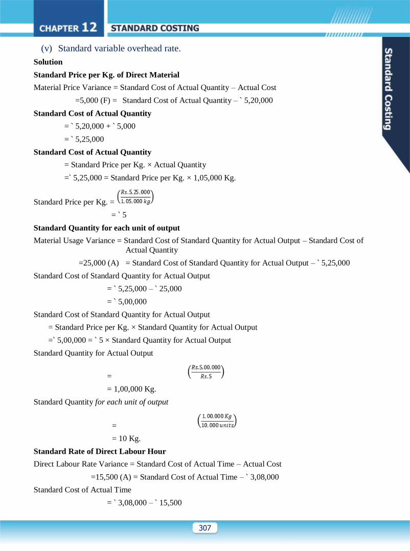
Solution
Standard Price per Kg. of Direct Material
Material Price Variance = Standard Cost of Actual Quantity – Actual Cost
=5,000 (F) = Standard Cost of Actual Quantity – ` 5,20,000
Standard Cost of Actual Quantity
= ` 5,20,000 + ` 5,000
= ` 5,25,000
Standard Cost of Actual Quantity
= Standard Price per Kg. × Actual Quantity
=` 5,25,000 = Standard Price per Kg. × 1,05,000 Kg.
Standard Price per Kg. =
= ` 5
Standard Quantity for each unit of output
Material Usage Variance = Standard Cost of Standard Quantity for Actual Output – Standard Cost of
Actual Quantity
=25,000 (A) = Standard Cost of Standard Quantity for Actual Output – ` 5,25,000
Standard Cost of Standard Quantity for Actual Output
= ` 5,25,000 – ` 25,000
= ` 5,00,000
Standard Cost of Standard Quantity for Actual Output
= Standard Price per Kg. × Standard Quantity for Actual Output
=` 5,00,000 = ` 5 × Standard Quantity for Actual Output
Standard Quantity for Actual Output
=
= 1,00,000 Kg.
Standard Quantity for each unit of output
=
= 10 Kg.
Standard Rate of Direct Labour Hour
Direct Labour Rate Variance = Standard Cost of Actual Time – Actual Cost
=15,500 (A) = Standard Cost of Actual Time – ` 3,08,000
Standard Cost of Actual Time
= ` 3,08,000 – ` 15,500
Page 16
308
= ` 2,92,500
Standard Cost of Actual Time
= Standard Rate per hr. × Actual Hours
=` 2,92,500 = Standard Rate per hr. × 19,500 hrs
Standard Rate per hr. =
= ` 15
Standard Time for Actual Production
Labour Efficiency Variance = Standard Cost of Standard Time for Actual Production – Standard Cost
of Actual Time
=7,500 (F) = Standard Cost of Standard Time for Actual Production –
` 2,92,500
Standard Cost of Standard Time for Actual Production
= ` 2,92,500 + ` 7,500
= ` 3,00,000
Standard Cost of Standard Time for Actual Production
= Standard Rate per hr. × Standard Time for Actual Production
=` 3,00,000 = ` 15 × Standard Time for Actual Production Standard Time for Actual Production
=
= 20,000hrs
Standard Variable Overhead Rate
Variable Overhead Variance = Standard Variable Overheads for Production – Actual Variable
Overheads
=10,000 (A) = Standard Variable Overheads for Production – ` 4,10,000
Standard Variable Overheads for Production
= ` 4,10,000 – ` 10,000
= ` 4,00,000
Standard Variable Overheads for Production
= Standard Variable Overhead Rate per Unit × Actual Production (Units)
= ` 4,00,000 = Standard Variable Overhead Rate per Unit × 10,000 units
Standard Variable Overhead Rate per unit
=
= ` 40
Or
Standard Variable Overheads for Production
= Standard Variable Overhead Rate per Hour × Standard Hours for Actual Production
Page 17
309
=` 4,00,000 = Standard Variable Overhead Rate per Hour × 20,000 hrs
Standard Variable Overhead Rate per hour
=
= ` 20
Sales Variance
Question 25:Compute the missing data indicated by the question marks from the
following:
Product R Product S
Standard Sales Qty. (Units) ??? 400
Actual Sales Qty. (Units) 500 ???
Standard Price/Unit `12 `15
Actual Price/Unit `15 `20
Sales Price Variance ??? ???
Sales Volume Variance `1,200 (F) ???
Sales Value Variance ??? ???
Sales Mix Variance for both the products together was `450 (F). ‘F’ denote favourable.
Solution:
Statement Showing “Standard & Actual Data (incomplete)”
Product Standard / Budgeted Data Actual Data
Qty.
(units)
Price
(per unit)
Amount
(`)
Qty.
(units)
Price
(per unit)
Amount
(`)
R ? ?? ` 12 ??? 500 ` 15 7,500
S 400 ` 15 6,000 ??? ` 20 ???
Total ??? ? ?? ? ?? ???
Product: R
Sales Price Variance = Actual Qty. × (Actual Price – Budgeted Price)
= 500 units × (` 15 – ` 12)
= ` 1,500 (F)
Sales Volume Variance = Budgeted Price × (Actual Qty. – Budgeted Qty.)
Page 18
310
`1,200 (F) = ` 12 × (500 units – Budgeted Qty.)
= Budgeted Qty. = 400 units
Sales Value Variance = Sales Price Variance + Sales Volume Variance
= ` 1,500 (F) + ` 1,200 (F)
= ` 2,700 (F)
The table can now be presented as follows. Assumed Actual Quantity of S is ‘T’ units.
Product Standard / Budgeted Data Actual Data
Qty.
(units)
Price
(per unit)
Amount
(`)
Qty.
(units)
Price
(per unit)
Amount
(`)
R 400 ` 12 4,800 500 ` 15 7,500
S 400 ` 15 6,000 T ` 20 20 x T
800 10,800 500 + T 7,500 + 20T
Sales Mix Variance = Total Actual Qty (units) × (Average Budgeted Price per unit of Actual Mix –
Average Budgeted Price per unit of Budgeted Mix)
=`450 (F) = (500 units + T units) ×
=`450 (F) = 6,000 +15T– 13.5 × (500 + T)
=T = 800 units
Statement Showing “Standard & Actual Data (Complete)”
Product Standard / Budgeted Data Actual Data
Qty.
(units)
Price
(per unit)
Amount
(`)
Qty.
(units)
Price
(per unit)
Amount
(`)
R 400 ` 12 4,800 500 ` 15 7,500
S 400 ` 15 6,000 800 ` 20 16,000
800 10,800 1,300 23,500
Product: S
Sales Price Variance = Actual Qty. × (Actual Price – Budgeted Price)
= 800 units × (` 20 – ` 15)
= ` 4,000 (F)
Sales Volume Variance = Budgeted Price × (Actual Qty. – Budgeted Qty.)
= ` 15 × (800 units – 400 units)
= ` 6,000 (F)
Page 19
311
Sales Value Variance = Sales Price Variance + Sales Volume Variance
= 4,000 (F) + 6,000 (F)
= `10,000 (F)
Planning and Operational variances for Sales
The Sales volume variance can be sub-divided into a planning and operational variance:
Actual sales quantity × Standard margin
Market Share variance (Operational)
Revised budgeted sales × Standard margin
(to achieve target share of actual market )
Market size variance(planning)
Original budgeted sales × standard margin
Computation of Variances and
Reconciliation of Budgeted/Standard Profit with Actual Profit
Question 28:Safron products Ltd. produces and sells a single product. Standard cost
card per unit of the product is as follows.
`
Direct Material, A 10 kg @ `5 per kg 50.00
B 5 kg @ `6 per kg 30.00
Direct Wages, 5 hours @ ` 5 per hour 25.00
Variable Production Overheads, 5 hours @ 12 per hour 60.00
Fixed Production Overheads 25.00
Total Standard Cost 190.00
Standard Gross Profit 35.00
Standard Selling Price 225.00
A fixed production overhead has been absorbed on the expected annual output of 25, 200
units produced evenly throughout the year. During the month of December, 2013, the
following were the actual results for an actual production of 2,000 units:
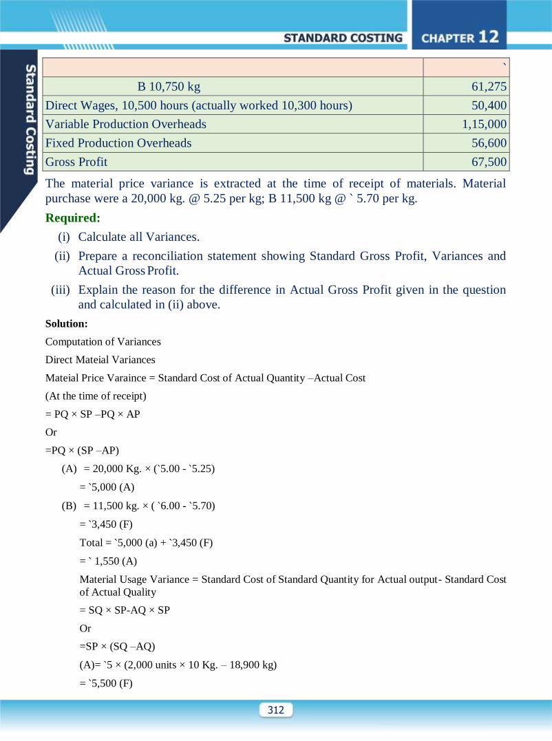
`
Sales, 2,000 units @ ` 225 4,50,000
Direct Materials, A 18,900 kg 99,225
Page 20
312
`
B 10,750 kg 61,275
Direct Wages, 10,500 hours (actually worked 10,300 hours) 50,400
Variable Production Overheads 1,15,000
Fixed Production Overheads 56,600
Gross Profit 67,500
The material price variance is extracted at the time of receipt of materials. Material
purchase were a 20,000 kg. @ 5.25 per kg; B 11,500 kg @ ` 5.70 per kg.
Required:
(i) Calculate all Variances.
(ii) Prepare a reconciliation statement showing Standard Gross Profit, Variances and
Actual Gross Profit.
(iii) Explain the reason for the difference in Actual Gross Profit given in the question
and calculated in (ii) above.
Solution:
Computation of Variances
Direct Mateial Variances
Mateial Price Varaince = Standard Cost of Actual Quantity –Actual Cost
(At the time of receipt)
= PQ × SP –PQ × AP
Or
=PQ × (SP –AP)
(A) = 20,000 Kg. × (`5.00 - `5.25)
= `5,000 (A)
(B) = 11,500 kg. × ( `6.00 - `5.70)
= `3,450 (F)
Total = `5,000 (a) + `3,450 (F)
= ` 1,550 (A)
Material Usage Variance = Standard Cost of Standard Quantity for Actual output- Standard Cost
of Actual Quality
= SQ × SP-AQ × SP
Or
=SP × (SQ –AQ)
(A)= `5 × (2,000 units × 10 Kg. – 18,900 kg)
= `5,500 (F)
Page 21
313
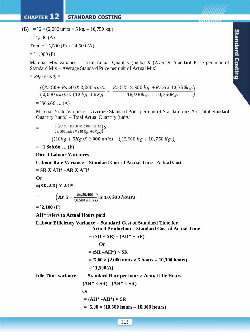
(B) = `6 × (2,000 units × 5 kg. – 10,750 kg.)
= `4,500 (A)
Total = ` 5,500 (F) + ` 4,500 (A)
= ` 1,000 (F)
Material Mix variance = Total Actual Quantity (units) X (Average Standard Price per unir of
Standard Mix – Average Standard Price per unit of Actual Mix)
= 29,650 Kg. ×
= `866.66…..(A)
Material Yield Variance = Average Standard Price per unit of Standard mix X ( Total Standard
Quantity (units) – Total Actual Quantity (units)
= X
= ` 1,866.66…. (F)
Direct Labour Variances
Labour Rate Variance = Standard Cost of Actual Time –Actual Cost
= SR X AH* –AR X AH*
Or
=(SR-AR) X AH*
=
= `2,100 (F)
AH* refers to Actual Hours paid
Labour Efficiency Variance = Standard Cost of Standard Time for
Actual Production – Standard Cost of Actual Time
= (SH × SR) – (AH* × SR)
Or
= (SH –AH*) × SR
= `5.00 × (2,000 units × 5 hours – 10,300 hours)
= ` 1,500(A)
Idle Time variance = Standard Rate per hour × Actual idle Hours
= (AH* × SR) - (AH* × SR)
Or
= (AH* -AH*) × SR
= `5.00 × (10,500 hours – 10,300 hours)
Page 22
314
= `1,000 (A)
AH* refers to Actual Hours Worked
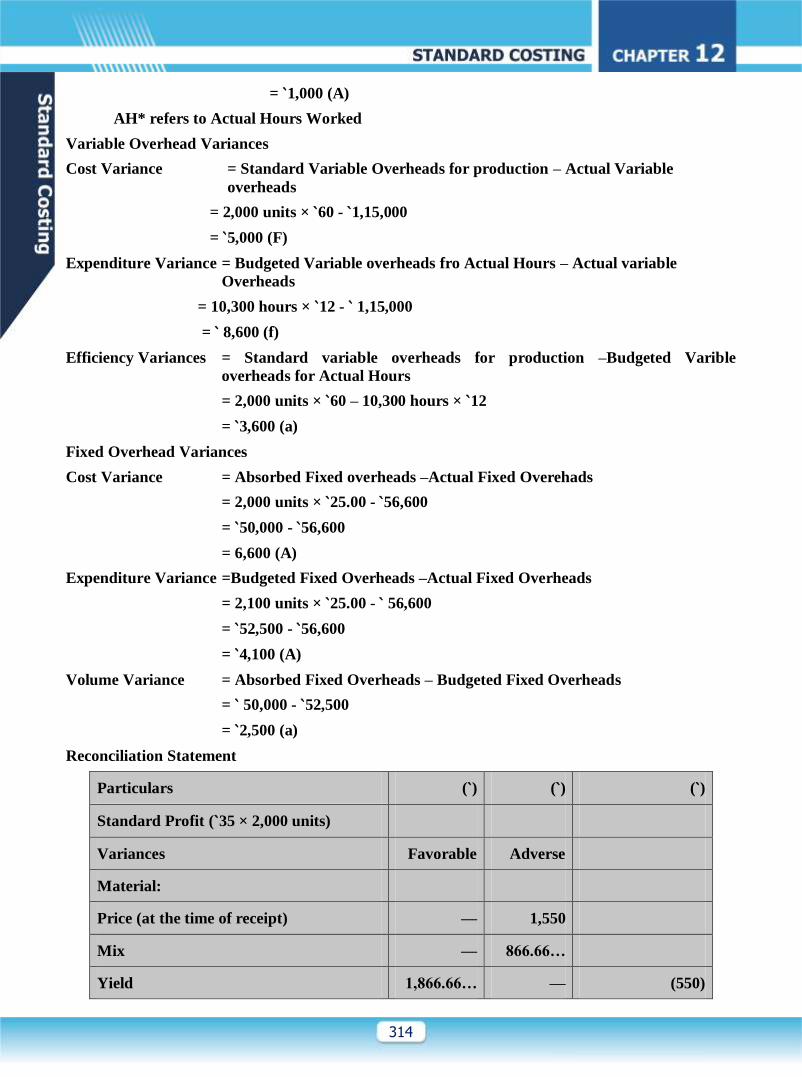
Variable Overhead Variances
Cost Variance = Standard Variable Overheads for production – Actual Variable
overheads
= 2,000 units × `60 - `1,15,000
= `5,000 (F)
Expenditure Variance = Budgeted Variable overheads fro Actual Hours – Actual variable
Overheads
= 10,300 hours × `12 - ` 1,15,000
= ` 8,600 (f)
Efficiency Variances = Standard variable overheads for production –Budgeted Varible
overheads for Actual Hours
= 2,000 units × `60 – 10,300 hours × `12
= `3,600 (a)
Fixed Overhead Variances
Cost Variance = Absorbed Fixed overheads –Actual Fixed Overehads
= 2,000 units × `25.00 - `56,600
= `50,000 - `56,600
= 6,600 (A)
Expenditure Variance =Budgeted Fixed Overheads –Actual Fixed Overheads
= 2,100 units × `25.00 - ` 56,600
= `52,500 - `56,600
= `4,100 (A)
Volume Variance = Absorbed Fixed Overheads – Budgeted Fixed Overheads
= ` 50,000 - `52,500
= `2,500 (a)
Reconciliation Statement
Particulars (`) (`) (`)
Standard Profit (`35 × 2,000 units)
Variances Favorable Adverse
Material:
Price (at the time of receipt) — 1,550
Mix — 866.66…
Yield 1,866.66… — (550)
Page 23
315
Particulars (`) (`) (`)
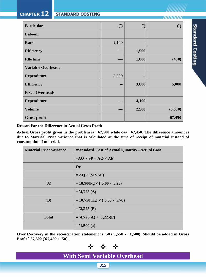
Labour:
Rate 2,100 —
Efficiency — 1,500
Idle time — 1,000 (400)
Variable Overheads
Expenditure 8,600 --
Efficiency -- 3,600 5,000
Fixed Overheads.
Expenditure --- 4,100
Volume --- 2,500 (6,600)
Gross profit 67,450
Reason For the Difference in Actual Gross Profit
Actual Gross profit given in the problem is ` 67,500 while cas ` 67,450. The difference amount is
due to Material Price variance that is calculated at the time of receipt of material instead of
consumption if material.
Material Price variance =Standard Cost of Actual Quantity –Actual Cost
=AQ × SP – AQ × AP
Or
= AQ × (SP-AP)
(A) = 18,900kg × (`5.00 - `5.25)
= `4,725 (A)
(B) = 10,750 Kg. × (`6.00 - `5.70)
= `3,225 (F)
Total = `4,725(A) + `3,225(F)
= `1,500 (a)
Over Recovery in the reconciliation statement is `50 (`1,550 - ` 1,500). Should be added in Gross
Profit ` 67,500 (`67,450 + `50).
With Semi Variable Overhead
Page 24
316
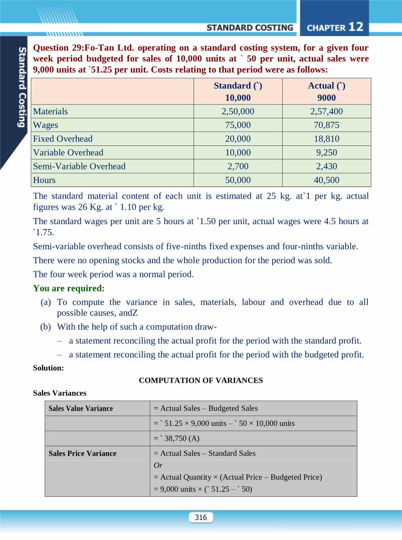
Question 29:Fo-Tan Ltd. operating on a standard costing system, for a given four
week period budgeted for sales of 10,000 units at ` 50 per unit, actual sales were
9,000 units at `51.25 per unit. Costs relating to that period were as follows:
Standard (`)
10,000
Actual (`)
9000
Materials 2,50,000 2,57,400
Wages 75,000 70,875
Fixed Overhead 20,000 18,810
Variable Overhead 10,000 9,250
Semi-Variable Overhead 2,700 2,430
Hours 50,000 40,500
The standard material content of each unit is estimated at 25 kg. at`1 per kg. actual
figures was 26 Kg. at ` 1.10 per kg.
The standard wages per unit are 5 hours at `1.50 per unit, actual wages were 4.5 hours at
`1.75.
Semi-variable overhead consists of five-ninths fixed expenses and four-ninths variable.
There were no opening stocks and the whole production for the period was sold.
The four week period was a normal period.
You are required:
(a) To compute the variance in sales, materials, labour and overhead due to all
possible causes, andZ
(b) With the help of such a computation draw-
– a statement reconciling the actual profit for the period with the standard profit.
– a statement reconciling the actual profit for the period with the budgeted profit.
Solution:
COMPUTATION OF VARIANCES
Sales Variances
Sales Value Variance = Actual Sales – Budgeted Sales
= ` 51.25 × 9,000 units – ` 50 × 10,000 units
= ` 38,750 (A)
Sales Price Variance = Actual Sales – Standard Sales
Or
= Actual Quantity × (Actual Price – Budgeted Price)
= 9,000 units × (` 51.25 – ` 50)
Page 25
317
= 11,250 (F)
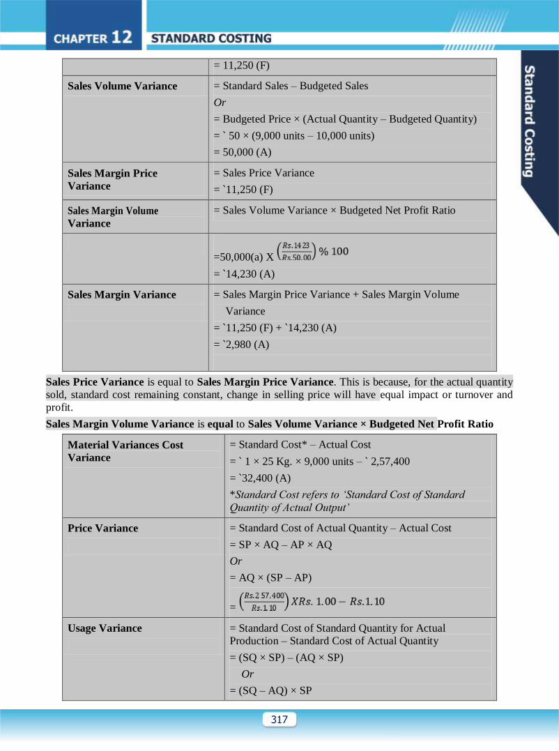
Sales Volume Variance = Standard Sales – Budgeted Sales
Or
= Budgeted Price × (Actual Quantity – Budgeted Quantity)
= ` 50 × (9,000 units – 10,000 units)
= 50,000 (A)
Sales Margin Price
Variance
= Sales Price Variance
= `11,250 (F)
Sales Margin Volume
Variance
= Sales Volume Variance × Budgeted Net Profit Ratio
=50,000(a) X
= `14,230 (A)
Sales Margin Variance
= Sales Margin Price Variance + Sales Margin Volume
Variance
= `11,250 (F) + `14,230 (A)
= `2,980 (A)
Sales Price Variance is equal to Sales Margin Price Variance. This is because, for the actual quantity
sold, standard cost remaining constant, change in selling price will have equal impact or turnover and
profit.
Sales Margin Volume Variance is equal to Sales Volume Variance × Budgeted Net Profit Ratio
Material Variances Cost
Variance
= Standard Cost* – Actual Cost
= ` 1 × 25 Kg. × 9,000 units – ` 2,57,400
= `32,400 (A)
*Standard Cost refers to ‘Standard Cost of Standard
Quantity of Actual Output’
Price Variance
= Standard Cost of Actual Quantity – Actual Cost
= SP × AQ – AP × AQ
Or
= AQ × (SP – AP)
=
Usage Variance
= Standard Cost of Standard Quantity for Actual
Production – Standard Cost of Actual Quantity
= (SQ × SP) – (AQ × SP)
Or
= (SQ – AQ) × SP
Page 26
318
=
= `9,000 (A)
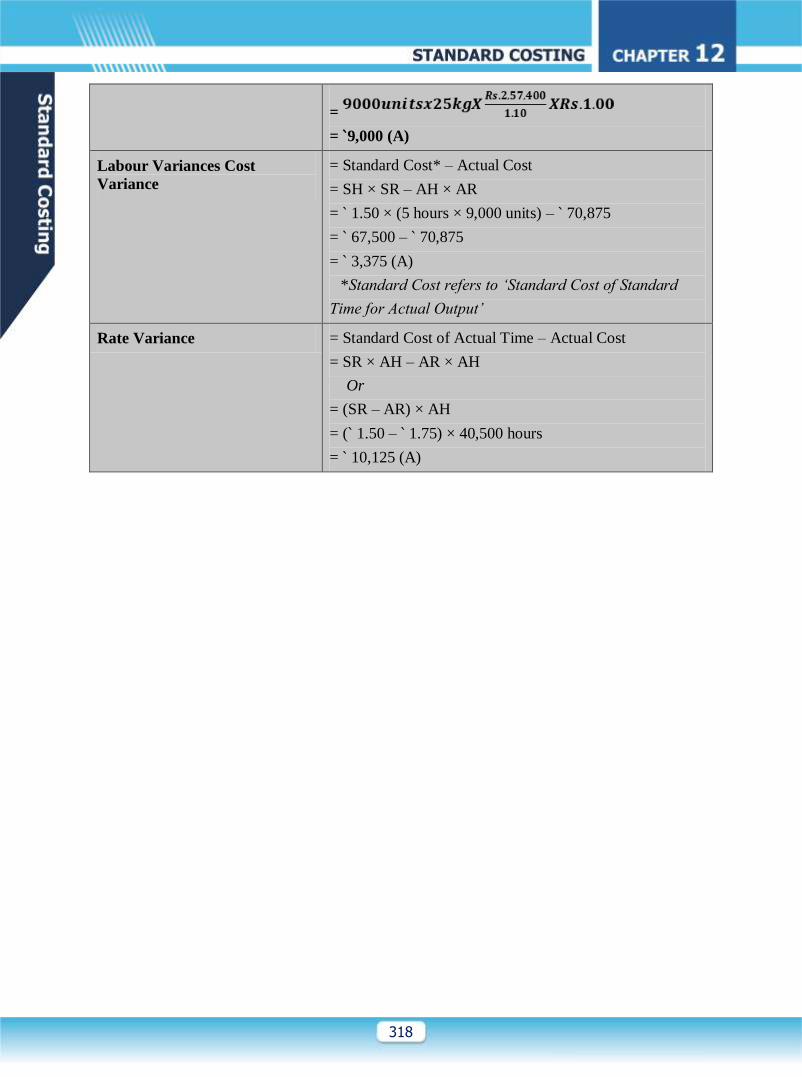
Labour Variances Cost
Variance
= Standard Cost* – Actual Cost
= SH × SR – AH × AR
= ` 1.50 × (5 hours × 9,000 units) – ` 70,875
= ` 67,500 – ` 70,875
= ` 3,375 (A)
*Standard Cost refers to ‘Standard Cost of Standard
Time for Actual Output’
Rate Variance = Standard Cost of Actual Time – Actual Cost
= SR × AH – AR × AH
Or
= (SR – AR) × AH
= (` 1.50 – ` 1.75) × 40,500 hours
= ` 10,125 (A)
Page 27
319
Efficiency Variance = Standard Cost of Standard Time for Actual Production –
Standard Cost of Actual Time
= (SH × SR) – (AH × SR)
Or
= (SH – AH) × SR
= (45,000 hours – 40,500 hours) × ` 1.50
= ` 6,750 (F)
4. Variable Overhead Cost Variances
Cost Variance = Standard Variable Overheads for Production – Actual
Variable Overheads
= `1.12 × 9,000 units – `10,330
= ` 250 (A)
Expenditure Variance = Budgeted Overheads for Actual Hours – Actual
Overheads
= 40,500 hours × ` 0.224 – ` 10,330
= ` 1,258 (A)
Efficiency Variance
= Standard Variable Overheads for Production – Budgeted
Overheads for Actual Hours
= `1.12 × 9,000 units – 40,500 hours × ` 0.224
= ` 1,008 (F)
5. Fixed Overhead Variances
Cost Variance = Absorbed Fixed Overheads – Actual Fixed Overheads
= 9,000 units × ` 2.15 – ` 20,160
= ` 19,350 – ` 20,160
= ` 810 (A)
Expenditure Variance = Budgeted Fixed Overheads – Actual Fixed Overheads
= ` 21,500 – ` 20,160
= ` 1,340 (F)
Volume Variance = Absorbed Fixed Overheads – Budgeted Fixed
Overheads
= ` 19,350 – ` 21,500
= ` 2,150 (A)
Page 28
320
Capacity Variance = Budgeted Fixed Overheads for Actual Hours –
Budgeted Fixed Overheads
= 40,500 hours × ` 0.43 – ` 21,500
= ` 4,085 (A)
Efficiency Variance = Absorbed Fixed Overheads – Budgeted Fixed
Overheads for Actual Hours
= ` 19,350 – 40,500 hours × ` 0.43
= ` 1,935 (F)
RECONCILIATION STATEMENT
(Standard and Actual Profit)
Particulars (`) (`)
Profit- Standard 1,28,070
Sales Margin Variances
Volume N.A.
Price 11,250 (F) 11,250
Direct Material Variances
Price 23,400 (A)
Usage 9,000 (A) (32,400)
Direct Labour Variances
Labour Rate 10,125 (A)
Labour Efficiency 6,750 (F) (3,375)
Variable Overhead Variances
Expenditure 1,258 (A)
Efficiency 1,008 (F) (250)
Fixed Overhead Variances
Expenditure 1,340 (F)
Capacity 4,085 (A)
Efficiency 1,935 (F) (810)
Actual Profit 1,02,485
RECONCILIATION STATEMENT
(Budgeted & Actual Profit)
Particulars (`) (`)
Page 29
321
Budgeted Profit (10,000 units x ` 14.23) 1,42,300
Sales Margin Variances
Volume 14,230 (A)
Price 11,250 (F) (2,980)
Direct Material Variances
Price 23,400 (A)
Usage 9,000 (A) (32,400)
Direct Labour Variances
Labour Rate 10,125 (A)
Labour Efficiency 6,750 (F) (3,375)
Variable Overhead Variances
Expenditure 1,258 (A)
Efficiency 1,008 (F) (250)
Fixed Overhead Variances
Expenditure 1,340 (F)
Capacity 4,085 (A)
Efficiency 1,935 (F) (810)
Actual Profit 1,02,485
WORKING NOTES
Standard Variable Overheads = ` 10,000 + ` 2,700 × 4/9
= ` 11,200
Std. Variable Overhead Rate per unit
=
= `1.12
Std. Variable Overheads Rate per
hour =
= ` 0.224
Actual Variable Overheads = ` 9,250 + ` 2,430 × 4/9
= ` 10,330
Budgeted Fixed Overheads = ` 20,000 + 5/9 × ` 2,700
= ` 21,500
Page 30
322
Standard Fixed Overheads Rate per
unit =
=Rs. 2.15
Std. Fixed Overheads Rate per hour
= ` 0.43
Actual Fixed Overheads = ` 18,810 + ` 2,430 × 5/9
= ` 20,160
Standard Hrs. for actual production
= 9,000 units ×
= 45,000 hours
Standard Cost per unit
=
= `35.77
Budgeted Margin per unit = `50 – `35.77
= `14.23
Standard Profit/Margin = Actual Qty. Sold × Budgeted Margin per unit
= 9,000 units × ` 14.23
= `1,28,070
Computation of Actual Profit
Actual Sales (9,000 units × ` 51.25)
Actual Cost of Sales
Actual Profit
= ` 4,61,250
= ` 3,58,765
= Actual Sales – Actual Cost of Sales
= ` 4,61,250 – ` 3,58,765
= `1,02,485
Question 30:BOM & CO. operate a system of standard costs. For the four weeks
ended 31st March, 2013 the Following was their profit and Loss Account:
Particulars ` Particulars `
Material Consumed 1,89,000 Transfer to Sales Deptt. 3,500
units of Finished articles at. `140
each
4,90,000
Direct Wages 22,100
Fixed Expenses 1,88,000
Page 31
323
Variable Expenses 62,000
Profit 28,900
4,90,000 4,90,000
The following Further information is given:
(a) There was no opening or closing work-in-progress. The articles manufactured are
identical and get transferred to sales department after manufacture.
(b) Materials were drawn for 3,600 units at ` 52.50 per unit.
(c) For the four week period, the standard production capacity is 4,800 units, and the
break-up of the standard selling prices is given below:
` Per unit
Material 50
Direct Wages 6
Fixed Expenses 40
Variable Expenses 20
Standard Cost of Sale 116
Standard Profit 24
Standard Selling Price 140
(d) The standard wages per article is based on 9,600 hours worked for the four-week
period at a rate of ` 3.00 per hour. 6,400 hours were actually worked during the
four-week period and, in addition, wages for 400 hours were paid to compensate
for idle time due to breakdown of a machine, and the overall wage rate was `3.25.
You have to present a Trading and profit and loss account indicating the comparison
between standards and actual and analyse the variances.
Solution
COMPARISON BETWEEN STANDARD AND ACTUAL
Trading and Profit and Loss Account for 4 weeks ended 31st March, 2013
Particulars Std.
3,500
units
Actual
3,500
units
Variance Particulars Std.
3,500
units
Actual
3,500
units
Variance
` ` ` ` ` `
Material 1,75,000 1,89,000 14,000(A) Transfer to
Sales Dept.
at `140 each
4,90,000 4,90,000 -
Page 32
324
Particulars Std.
3,500
units
Actual
3,500
units
Variance Particulars Std.
3,500
units
Actual
3,500
units
Variance
` ` ` ` ` `
Direct
Wages
21,000 22,100 1,100(A)
Variable Exp. 70,000 62,000 8,000(F)
Fixed Exp. 1,40,000 1,88,000 48,000(A)
Profit 84,000 28,900 55,100(A)
4,90,000 4,90,000 4,90,000 4,90,000
COMPUTATION OF VARIANCES
1. Direct Material Variances
Material Price Variance = Actual Quantity × (Standard Price – Actual Price)
= 3,600 units × (` 50.00 – ` 52.50)
= ` 9,000 (A)
Material Usage Variance = Standard Price × (Standard Quantity – Actual Quantity)
= ` 50 × (3,500 units – 3,600 units)
= ` 5,000 (A)
Material Cost Variance = ` 9,000 (A) + ` 5,000 (A)
= `14,000 (A)
2. Direct Labour Cost Variance
Labour Rate Variance = Actual Hours × (Standard Rate – Actual Rate)
= 6,800 hours × (` 3.00 – ` 3.25)
= ` 1,700 (A)
Page 33
325
Labour Efficiency
Variance
= Standard Rate × (Standard Hours – Actual Hours)
= ` 3 × (3,500 units × 2 hours – 6,400 hours)
= ` 1,800 (F)
Idle Time Variance = Standard Rate × Idle Hours
= ` 3 × 400
= ` 1,200 (A)
Labour Cost Variance = ` 1,700 (A) + ` 1,800 (F) + ` 1,200 (A)
= ` 1,100 (A)
3. Variable Expense Variance
= Standard Variable Expenses – Actual Variable Expenses
= 3,500 units × ` 20 – ` 62,000
= ` 8,000 (F)
4. Fixed Expenses Variances
Expenditure Variance = Budgeted Fixed Expenses – Actual Fixed Expenses
= 4,800 units × ` 40 – ` 1,88,000
= ` 4,000 (F)
Volume Variance = Absorbed Fixed Expenses – Budgeted Fixed Expenses
= ` 40 × 3,500 units – ` 40 × 4,800 units
= ` 52,000 (A)
Capacity Variance = Std. Rate per hour × (Actual Hours – Budgeted Hours)
= ` 20 × (6,400 hours – 9,600 hours)
= ` 64,000 (A)
Efficiency Variance
= Std. Rate per hour × (Std. Hours for Actual Output – Actual
Hours)
= ` 20 × (7,000 hours – 6,400 hours)
= ` 12,000 (F)
Fixed Expense
Variance
=` 4,000 (F) + ` 64,000 (A) + ` 12,000 (F)
= ` 48,000 (A)
Total Cost Variance = Direct Material Cost Variance + Direct Labour Cost Variance +
Variable Expenses Variance + Fixed Expenses Variance
= ` 14,000 (A) +1,100 (A) + ` 8,000 (F) + ` 48,000 (A)
= ` 55,100 (A)
6. Profit Variance = Standard Profit – Actual Profit
= ` 84,000 – ` 28,900
= ` 55,100 (A)
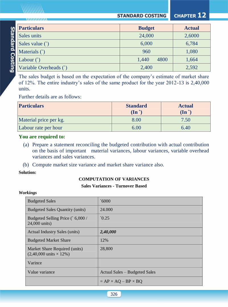
Question 33:Young Chin limited uses standard and marginal costing system. It
provides the following details for the year 2012-13 relating to its production, cost
and sales:
Page 34
326
Particulars Budget Actual
Sales units 24,000 2,6000
Sales value (`) 6,000 6,784
Materials (`) 960 1,080
Labour (`) 1,440 4800 1,664
Variable Overheads (`) 2,400 2,592
The sales budget is based on the expectation of the company’s estimate of market share
of 12%. The entire industry’s sales of the same product for the year 2012-13 is 2,40,000
units.
Further details are as follows:
Particulars Standard
(In `) Actual
(In `)
Material price per kg. 8.00 7.50
Labour rate per hour 6.00 6.40
You are required to:
(a) Prepare a statement reconciling the budgeted contribution with actual contribution
on the basis of important material variances, labour variances, variable overhead
variances and sales variances.
(b) Compute market size variance and market share variance also.
Solution:
COMPUTATION OF VARIANCES
Sales Variances - Turnover Based
Workings
Budgeted Sales `6000
Budgeted Sales Quantity (units) 24.000
Budgeted Selling Price (` 6,000 /
24,000 units)
`0.25
Actual Industry Sales (units) 2,40,000
Budgeted Market Share 12%
Market Share Required (units)
(2,40,000 units × 12%)
28,800
Varince
Value variance Actual Sales – Budgeted Sales
= AP × AQ – BP × BQ
Page 35
327
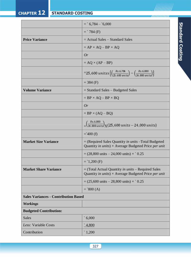
= ` 6,784 – `6,000
= ` 784 (F)
Price Variance = Actual Sales – Standard Sales
= AP × AQ – BP × AQ
Or
= AQ × (AP – BP)
=
= 384 (F)
Volume Variance = Standard Sales – Budgeted Sales
= BP × AQ – BP × BQ
Or
= BP × (AQ – BQ)
= X
=`400 (f)
Market Size Variance = (Required Sales Quantity in units –Total Budgeted
Quantity in units) × Average Budgeted Price per unit
= (28,800 units – 24,000 units) × ` 0.25
= `1,200 (F)
Market Share Variance = (Total Actual Quantity in units – Required Sales
Quantity in units) × Average Budgeted Price per unit
= (25,600 units – 28,800 units) × ` 0.25
= `800 (A)
Sales Variances - Contribution Based
Workings
Budgeted Contribution:
Sales ` 6,000
Less: Variable Costs ` 4,800
Contribution ` 1,200
Page 36
328
Budgeted Units 24,000
Contribution / unit (`1,200 / 24,000
units)
` 0.05
Page 37
329
Variances
Sales Contribution Price Variance
= Sales Price Variance
= 384 (F)
Sales Contribution Volume Variance = Sales Volume Variance x Budgeted Profit
Volume Ratio
=400(F) X
= ` 80 (F)
Market Size Variance = (Required Sales Quantity in units –Total
Budgeted Quantity in units) × Average Budgeted
Contribution per unit
= (28,800 units – 24,000 units) × ` 0.05
= `240 (F)
Market Share Variance = (Total Actual Quantity in units – Required
Sales Quantity in units) × Average Budgeted
Contribution per unit
= (25,600 units – 28,800 units) × ` 0.05
= `160 (A)
Contribution Variance = Sales Contribution Price Variance + Sales
Contribution Volume Variance
= `384 (F) + `80 (F)
= `464 (F)
Direct Materials Variance
Workings
Budgeted Material Cost ` 960
Budgeted Units 24,000
Budgeted Material Cost per 100 units
(`960 / 24,000units × 100)
` 4
Standard Price of Material per Kg ` 8
Standard Requirement of Materials per
100 units of output (`4 / `8)
0.50 Kg
Actual Output (units) 25,600
Standard Requirement for Actual Output 128 Kg
Page 38
330
{(25,600 units × 0.50 Kg) / 100 units}
Actual Material Cost ` 1,080
Actual Price per Kg ` 7.50
Actual Quantity of Materials Consumed
(`1,080 / `7.50)
144 Kg
Variances
Material Price Variance = Standard Cost of Actual Quantity – Actual Cost
Or
= Actual Qty. × (Std. Price – Actual Price)
= 144 Kg. × (` 8 – ` 7.50)
= 72 (F)
Material Usage Variance Standard Cost of Standard Quantity for Actual
Production – Standard Cost of Actual Quantity
Or
= Std. Price × (Std. Qty. – Actual Qty.)
= ` 8 × (128 Kg. – 144 Kg.)
= ` 128 (A)
Direct Labour Variances
Workings
Budgeted Labour Cost ` 1,440
Budgeted Units 24,000
Budgeted Labour Cost per 100 units
(`1,440 / 24,000 units ×100 units)
` 6
Standard Labour Rate per hour ` 6
Standard Requirement of Labour Hours
per 100 units of output (`6 / `6)
1 hr
Actual Output (units) 25,600
Standard Hours Required for Actual
Output (25,600 units × 1 hr /100 units)
256 hrs
Actual Labour Cost ` 1,664
Actual Direct Labour Rate per hour ` 6.40
Actual Hours Worked (`1,664 / `6.40) 260 hrs
Budgeted Direct Labour Hours (`1,440 / 240 hrs
Page 39
331
`6)
Variances
Labour Rate Variance = Standard Cost of Actual Time – Actual Cost
Or
= Actual Hours × (Std. Rate – Actual Rate)
= 260 hours × (` 6.00 – ` 6.40)
= `104 (A)
Labour Efficiency Variance = Standard Cost of Standard Time for Actual
Production – Standard Cost of Actual Time
OR
= Std. Rate × (Std. Hours – Actual Hours)
= ` 6 × (256 hours – 260 hours)
= ` 24 (A)
Variable Overheads Variances
Workings
Budgeted Variable Overheads ` 2,400
Budgeted Labour Hours 240
Standard Variable Overhead Rate per
direct labour hour (` 2,400 / ` 240)
` 10
Actual Hours 260 hrs
Standard Hours Required for Actual
Output
256 hrs
Variances
Expenditure Variance = Budgeted Variable Overheads for Actual Hours
– Actual Variable Overheads
= 260 hours × ` 10 – ` 2,592
= ` 8 (F)
Efficiency Variances = Standard Variable Overheads for Production –
Budgeted Variable Overheads for Actual Hours
= 256 hours × ` 10 – 260 hours × ` 10
= 40 (A)
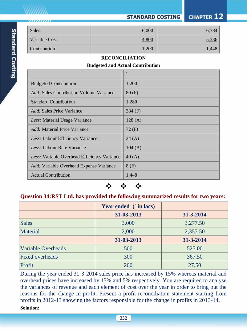
CONTRIBUTION ANALYSIS
Budget Actual
Page 40
332
Sales 6,000 6,784
Variable Cost 4,800 5,336
Contribution 1,200 1,448
RECONCILIATION
Budgeted and Actual Contribution
`
Budgeted Contribution 1,200
Add: Sales Contribution Volume Variance 80 (F)
Standard Contribution 1,280
Add: Sales Price Variance 384 (F)
Less: Material Usage Variance 128 (A)
Add: Material Price Variance 72 (F)
Less: Labour Efficiency Variance 24 (A)
Less: Labour Rate Variance 104 (A)
Less: Variable Overhead Efficiency Variance 40 (A)
Add: Variable Overhead Expense Variance 8 (F)
Actual Contribution 1,448
Question 34:RST Ltd. has provided the following summarized results for two years:
Year ended (` in lacs)
31-03-2013 31-3-2014
Sales 3,000 3,277.50
Material 2,000 2,357.50
31-03-2013 31-3-2014
Variable Overheads 500 525.00
Fixed overheads 300 367.50
Profit 200 27.50
During the year ended 31-3-2014 sales price has increased by 15% whereas material and
overhead prices have increased by 15% and 5% respectively. You are required to analyse
the variances of revenue and each element of cost over the year in order to bring out the
reasons for the change in profit. Present a profit reconciliation statement starting from
profits in 2012-13 showing the factors responsible for the change in profits in 2013-14.
Solution:
Page 41
333
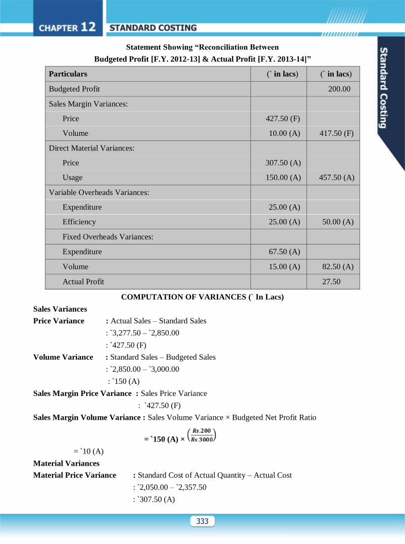
Statement Showing “Reconciliation Between
Budgeted Profit [F.Y. 2012-13] & Actual Profit [F.Y. 2013-14]”
Particulars (` in lacs) (` in lacs)
Budgeted Profit 200.00
Sales Margin Variances:
Price 427.50 (F)
Volume 10.00 (A) 417.50 (F)
Direct Material Variances:
Price 307.50 (A)
Usage 150.00 (A) 457.50 (A)
Variable Overheads Variances:
Expenditure 25.00 (A)
Efficiency 25.00 (A) 50.00 (A)
Fixed Overheads Variances:
Expenditure 67.50 (A)
Volume 15.00 (A) 82.50 (A)
Actual Profit 27.50
COMPUTATION OF VARIANCES (` In Lacs)
Sales Variances
Price Variance : Actual Sales – Standard Sales
: `3,277.50 – `2,850.00
: `427.50 (F)
Volume Variance : Standard Sales – Budgeted Sales
: `2,850.00 – `3,000.00
: `150 (A)
Sales Margin Price Variance : Sales Price Variance
: `427.50 (F)
Sales Margin Volume Variance : Sales Volume Variance × Budgeted Net Profit Ratio
= `150 (A) ×
= `10 (A)
Material Variances
Material Price Variance : Standard Cost of Actual Quantity – Actual Cost
: `2,050.00 – `2,357.50
: `307.50 (A)
Page 42
334
Material Usage Variance : Standard Cost of Standard Quantity for Actual Output – Standard Cost
of Actual Quantity
= `1,900 – `2,050
= `150 (A)
Variable Overhead Variances Expenditure Variance
= Budgeted Variable Overheads for Actual Hours – Actual Variable
Overheads
Or
= Std. Rate per unit × Expected Output for Actual Hours Worked – Actual
Variable Overheads
= `500 – `525
= `25 (A)
Efficiency Variances = Standard Variable Overheads for Production – Budgeted Variable
Overheads for Actual Hours
Or
= Std. Rate per unit × Actual Output – Std. Rate per unit × Expected
Output for Actual Hours Worked
= `475 – `500
= `25 (A)
Fixed Overhead Variances
Expenditure Variance = Budgeted Fixed Overheads – Actual Fixed Overheads.
= `300.00 – `367.50
= `67.50 (A)
Volume Variance = Absorbed Fixed Overheads – Budgeted Fixed Overheads
= `285 – `300
= `15 (A)
WORKING NOTES (` in lacs)
Note-1
Sales in F.Y. 2013-2014 3,277.50
Less: Increase due to price rise [`3,277.50 lacs × 15/115] 427.50
Sales in F.Y. 2013-2014 at F.Y. 2012-2013 Prices [Standard Sales] 2,850.00
Sales in F.Y. 2012-2013 3,000.00
Fall in Sales in F.Y. 2013-2014 [`3,000 lacs − `2,850 lacs] 150.00
Percentage fall 5%
Note-2
Material Cost In F.Y. 2012-2013 2,000.00
Less: 5% for Decrease in Volume 100.00
Page 43
335
‘Standard Material Usage’ at F.Y. 2012-13 Prices
(Standard Cost of Standard Quantity for Actual output)
1,900.00
Actual Material Cost F.Y. 2013-2014
Less: 15% Increase in Prices [`2,357.50 lakhs × 15/115]
2,357.50
307.50
Actual Materials Used, at F.Y. 2012-2013 Prices
(Standard Cost of Actual Quantity)
2,050.00
Note-3
Variable Overheads Cost in F.Y. 2012-13 500.00
Less: 5% due to fall in Volume of Sales in F.Y. 2013-14 25.00
"Standard Overheads for Production" in F.Y. 2013-14 475.00
Actual Variable Overheads Incurred in F.Y. 2013-14 525.00
Less: 5% for Increase in Price [`525 lacs × 5 / 105] 25.00
Amount Spent in F.Y. 2013-14 at F.Y. 2012-13 Prices
(Budgeted Variable Overheads for Actual Hours)
500.00
Note-4
Fixed Overheads Cost in F.Y. 2012-13 300.00
Less: 5% due to fall in Volume of Sales in F.Y. 2013-14 15.00
"Standard Overheads for Production" in F.Y. 2013-14.
(Absorbed Fixed Overheads)
285.00
This problem can also be solve by ‘Contribution’
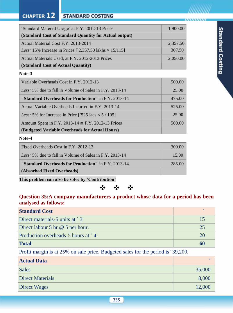
Question 35:A company manufacturers a product whose data for a period has been
analysed as follows:
Standard Cost `
Direct materials-5 units at ` 3 15
Direct labour 5 hr @ 5 per hour. 25
Production overheads-5 hours at ` 4 20
Total 60
Profit margin is at 25% on sale price. Budgeted sales for the period is` 39,200.
Actual Data `
Sales 35,000
Direct Materials 8,000
Direct Wages 12,000
Page 44
336
Analysis of variances
Adverse
` Favorable
`
Direct material
Price 800 —
Usage — 405
Direct Labour
Rate — 975
Efficiency 300 —
Production overhead
Expenditure 200 —
Volume — 340
Assume that there is no change in stock and that there are no other overheads.
Required:
To compute the following from the above details:
1. Sales price variance
2. Actual profit
3. Reconciliation between actual profit & budgeted profit.
4. Budgeted hours worked
5. Actual hours worked
6. Production overhead capacity variance
7. Actual production
8. Sales Volume profit variance
9. Production overhead efficiency variance
Answer:507 unit, ` 5000, 2595, 2450, 240A, 580F, 5560A, 340F, Budget profit= 9800,
490 unit.
Question 37:The working results of a Jems Ltd. For two corresponding years are
shown below:—
The working results of a Jems Ltd. For two corresponding years are shown below:—
Particulars Amount (` in Lakhs)
Page 45
337
Year 2012 Year 2013
Sales 600 770
Cost of Sales:
Direct materials 300 324
Direct wages and variable overheads 180 206
Fixed Overheads 80 150
Profit 40 90
In year 2013, there has been an increase in the selling price by 10 percent. Following are
the details of material consumption and utilization off direct labour hours during the two
years:
Particulars Year 2012 Year 2013
Direct materials Consumption (M.tons) 5,00,000 5,40,000
Direct Labour Hours 75,00,000 80,00,000
Required:—
Taking year 2012 as base year, analyse the variances of year 2013 and also workout the
amount which each variance has contributed to change in profit.
Find out the breakeven sales for both years.
Calculate the percentage increase in selling price in the year 2013 that would be needed
over the sale value of year 2013 to earn margin of safety of 45 per cent.
Solution
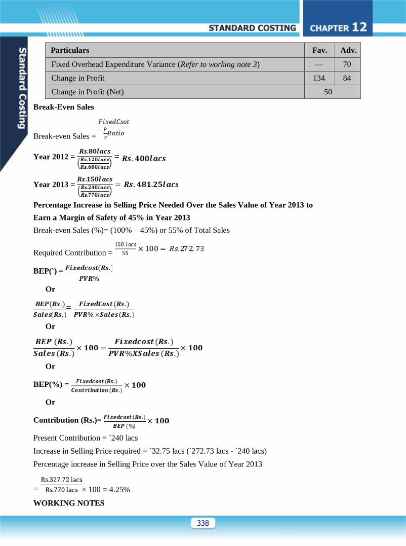
COMPUTATION OF REQUIREMENTS
Reconciliation Statement Showing “Factors Contributed Change in Profit”
(` in lacs)
Particulars Fav. Adv.
Increase in Contribution Due to Increase in Volume (` 140 lacs –`120 lacs)
(Refer to working note 3)
20 —
Sales Price Variance (Refer to working note 3) 70 —
Material Usage Variance (Refer to working note 4) 26 —
Material Price Variance (Refer to working note 4) — —
Direct Labour Rate Variance (Refer to working note 4) — 14
Direct Labour Efficiency Variance (Refer to working note 4) 18 —
Page 46
338
Particulars Fav. Adv.
Fixed Overhead Expenditure Variance (Refer to working note 3) — 70
Change in Profit 134 84
Change in Profit (Net) 50
Break-Even Sales
Break-even Sales =
Year 2012 = =
Year 2013 =
Percentage Increase in Selling Price Needed Over the Sales Value of Year 2013 to
Earn a Margin of Safety of 45% in Year 2013
Break-even Sales (%)= (100% – 45%) or 55% of Total Sales
Required Contribution =
BEP(`) =
Or
=
Or
Or
BEP(%) =
Or
Contribution (Rs.)=
Present Contribution = `240 lacs
Increase in Selling Price required = `32.75 lacs (`272.73 lacs - `240 lacs)
Percentage increase in Selling Price over the Sales Value of Year 2013
= × 100 = 4.25%
WORKING NOTES
Page 47
339
Budgeted Sales in Year 2013
If Actual Sales in Year 2013 is ` 110 then Budgeted Sales is ` 100.
If Actual Sales in Year 2013 is ` 1 then Budgeted Sales =
If Actual Sales in Year 2013 are ` 770,00,000 then Budgeted Sales are
= × 7,70,00,000 = `700 lacs
Budgeted Figures of Direct Material; Direct Wages; and Variable Overhead
Worked Out on the Basis of % of Sales in Year 2013
Direct Material % to Sales (in Year 2012) = × 300/600 × 100 = 50%
Budgeted figure of Direct Material (in Year 2013)
= 50% × ` 700 lacs = 350 lacs
Direct Wages and Variable Overhead (% to sales in Year 2012)
=
= 180/600 × 100 = 30%
Budgeted figure of Direct Wages and Variable Overhead (in Year 2013)
= 30% × 700 lacs = 210 lacs
Statement of Figures Extracted from Working Results of Company
(Figure in lacs of`)
Particulars Year
2012
[Actual]
(a)
Year
2013
[Budgeted]
(b)
Year
2013
[Actual]
(c)
Total
[Variance]
(d) = (c) –
(b)
Sales : (A)
(*Refer to working note 1)
600 700* 770 70 (F)
Direct Material...(a)*
( Refer to working note 2)
300 350*
324 26 (F)
Direct Wages and Variable Overhead...(b)*
( Refer to working note 2)
180 210
*
206 4 (F)
Total Variable Costs: (B) = (a + b) 480 560 530 30(F)
Contribution (C) = (A) – (B) 120 140 240 100 (F)
Less : Fixed Cost 80 80 150 70 (A)
Profit 40 60 90 30(F)
Page 48
340
Data for Material Variances (i)
Standard Cost for Actual Output Actual Cost
Quantity of
Material
(m/t)
Rate per
m/t
(`)
Amount
(`)
Quantity of
Material
(m/t)
Rate per
m/t
(`)
Amount
(`)
5,83,333..
*
60
350 lacs 5,40,000 60 324 lacs
300 lacs / 5 lacs m/t
Material Price Variance = (Standard Rate – Actual Rate) × Actual Quantity
= Nil
Material Usage Variance = (Standard Quantity – Actual Quantity) × Standard Rate per m/t
= (5,83,333.. – 5,40,000) × ` 60
= `26 lacs (F)
Data for Labour Variances/Overhead Variances (ii)
Standard Cost for Actual Output Actual Cost
Labour
Hours
Rate per
hour
(`)
Amount
(`)
Labour
Hours
Rate per
hour
(`)
Amount
(`)
87,50,000
2.40*
210 lacs 80,00,000 2.575 206 lacs
180 lacs / 75 lacs hours
Rate Variance = (Standard Rate – Actual Rate) × Actual Labour Hours
= (` 2.40 – ` 2.575) × 80,00,000
= `14 lacs (A)
Efficiency Variance = (Standard Labour Hours – Actual Labour Hours) × Standard Rate per Hour
= (87,50,000 – 80,00,000) × ` 2.40
= ` 18 lacs (F)
Question 43:Managing Director of Petro –Kl Ltd. (PTKLL) thinks that Standard Costing
has little to offer in the reporting of material variances due to frequently change in price
of materials.
PTKLL can utilize one for two equally suitable raw materials and always plan to utilize
the raw material which will lead to cheapest total production costs. However PTKLL is
Page 49
341
frequently trapped by price changes and the material actually used often provides, after
the event, to have been more expensive than the alternative which was originally rejected.
During Last accounting period, to produce a unit of “p” PTKLL could use either 2.50 Kf
of “PG” or 2.50 Kg of “PD” PTKLL planned to use “PG” as it appeared it would be
cheaper of the two and plans were based on a cost of “Pg” of ` 1.50 per Kg. Due to
market movements the actual prices changed and if PTKLL had purchased efficiently the
cost would have been:
“Pg” ` 2.25 per Kg.
“PD” ` 2.00 per Kg
Production of “P’ was 1,000 units and usage of “PG” amounted to 2,700 Kg at a total
cost of ` 6,480/-
You are required to analyze the material variance for “P’ by:
Traditional Variances Analysis: and
An approach which distinguishes between Planning and Operational Variances.
Solution:
COMPUTATION OF VARIANCES
Traditional Variance (Actual Vs Original Budget)
Usage Variance = (Standard Quantity – Actual Quantity) × Standard
Price
= (2,500 Kg – 2,700 Kg) × ` 1.50
= ` 300 (A)
Price Variance = (Standard Price – Actual Price) × Actual Quantity
= (` 1.50 – ` 2.40) × 2,700 Kg
= ` 2,430 (A)
Total Variance ` 300 (A) + ` 2,430 (A) = ` 2,730 (A)
Operational Variance (Actual Vs Revised)
Usage Variance = (2,500 Kg – 2,700 Kg) × ` 2.25
= ` 450 (A)
Price Variance = (` 2.25 – ` 2.40) × 2,700 Kg
= ` 405 (A)
Total Variance = ` 450 (A) + ` 405 (A) = ` 855 (A)
Planning Variance (Revised Vs Original Budget)
Controllable Variance = (` 2.00 – ` 2.25) × 2,500 Kg
= 625 (A)
Uncontrollable Variance = (` 1.50 – ` 2.00) × 2,500 kg
= 1,250 (a)
Page 50
342
Total Variance = ` 625 (A) + ` 1,250 (A) = ` 1,875 (A)
Traditional Variance = Operational Variance + Planning Variance
= 855 (A) + 1,875 (A) = 2,730 (A)
A Planning Variance simply compares a revised standard to the original standard. An Operational
Variance simply compares the actual results against the revised amount. Controllable Variances are
those variances which arises due to inefficiency of a cost centre /department. Uncontrollable Variances
are those variances which arises due to factors beyond the control of the management or concerned
department of the organization.
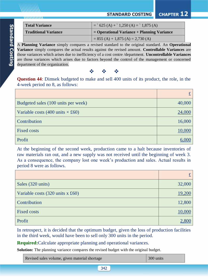
Question 44: Dimsek budgeted to make and sell 400 units of its product, the role, in the
4-week period no 8, as follows:
£
Budgeted sales (100 units per week) 40,000
Variable costs (400 units × £60) 24,000
Contribution 16,000
Fixed costs 10,000
Profit 6,000
At the beginning of the second week, production came to a halt because inventories of
raw materials ran out, and a new supply was not received until the beginning of week 3.
As a consequence, the company lost one week’s production and sales. Actual results in
period 8 were as follows.
£
Sales (320 units) 32,000
Variable costs (320 units x £60) 19,200
Contribution 12,800
Fixed costs 10,000
Profit 2,800
In retrospect, it is decided that the optimum budget, given the loss of production facilities
in the third week, would have been to sell only 300 units in the period.
Required:Calculate appropriate planning and operational variances.
Solution: The planning variance compares the revised budget with the original budget.
Revised sales volume, given material shortage 300 units
Page 51
343
Original budgeted sales volume 400 units
Planning variance in units of sales 100 units (A)
x standard contribution per unit x £40
Planning variance in £ £4,000 (A)
Arguably, running out of raw materials is an operational error and so the loss of sales volume and
contribution from the materials shortage is an opportunity cost that could have been avoided with better
purchasing arrangements. The operational variances are variances calculated in the usual way, except
that actual results are compared with the revised standard or budget. There is a sales volume
contribution variance which is an operational variance, as follows:
Actual sales volume 320 units
Revised sales volume 300 units
Operational sales volume variance in units
(possibly due to production efficiency or marketing efficiency)
20 units
x standard contribution per unit x £40
£800 (F)
These variances can be used as control information to reconcile budgeted and actual profit.
£ £
Operating statement, period 8
Budgeted profit 6,000
Planning variance 4,000 (A)
Operational variance – sales volume contribution 800 (F)
3,200 (A)
Actual profit in period 8 2,800
You will have noticed that in this example sales volume variances were valued at contribution forgone,
and there were no fixed cost volume variances. This is because contribution forgone, in terms of lost
revenue or extra expenditure incurred, is the nearest equivalent to opportunity cost that is readily
available to management accountants (who assume linearity of costs and revenues within a relevant
range of activity).
Question 47:Standard Costing – Reconciliation of Budgeted and Actual Profit
Osaka Manufacturing Co. (OMC) is a leading consumer goods company. The
budgeted and actual data of OMC for the year 2013-14 are as follows:—
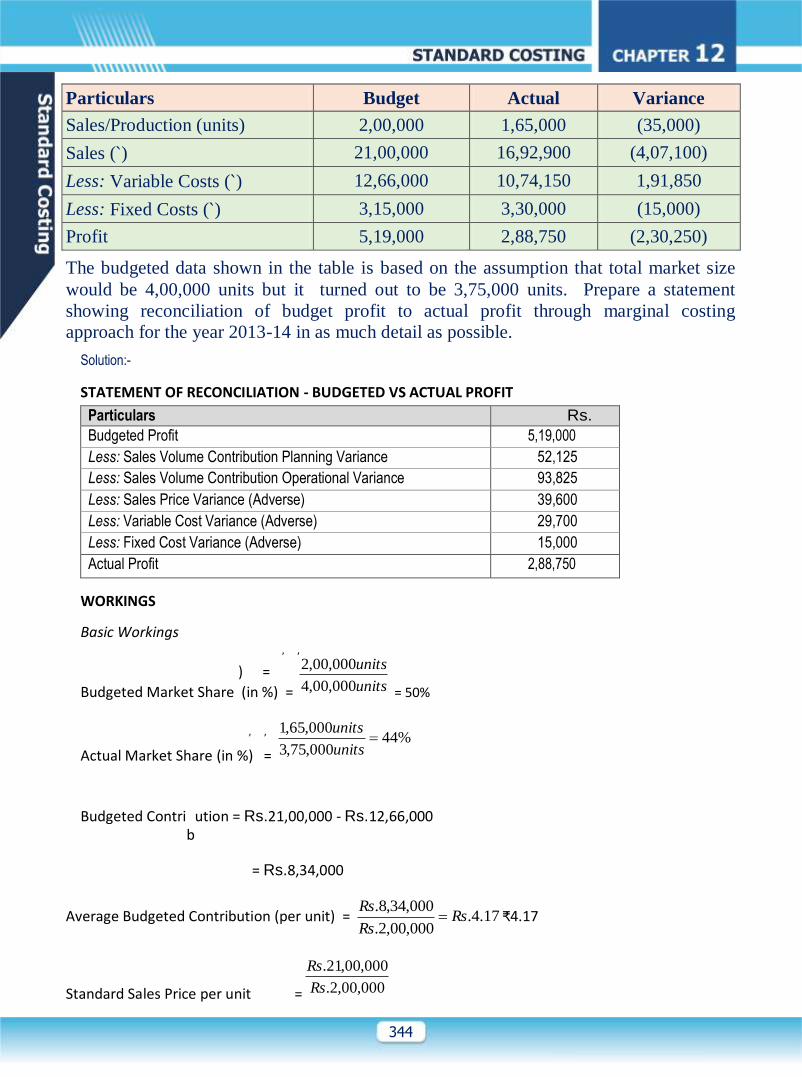
Particulars Budget Actual Variance
Page 52
344
,
,
,
, )
,
,
=
,
,
Particulars Budget Actual Variance
Sales/Production (units) 2,00,000 1,65,000 (35,000)
Sales (`) 21,00,000 16,92,900 (4,07,100)
Less: Variable Costs (`) 12,66,000 10,74,150 1,91,850
Less: Fixed Costs (`) 3,15,000 3,30,000 (15,000)
Profit 5,19,000 2,88,750 (2,30,250)
The budgeted data shown in the table is based on the assumption that total market size
would be 4,00,000 units but it turned out to be 3,75,000 units. Prepare a statement
showing reconciliation of budget profit to actual profit through marginal costing
approach for the year 2013-14 in as much detail as possible.
Solution:-
STATEMENT OF RECONCILIATION - BUDGETED VS ACTUAL PROFIT
Particulars Rs.
Budgeted Profit 5,19,000
Less: Sales Volume Contribution Planning Variance 52,125
Less: Sales Volume Contribution Operational Variance 93,825
Less: Sales Price Variance (Adverse) 39,600
Less: Variable Cost Variance (Adverse) 29,700
Less: Fixed Cost Variance (Adverse) 15,000
Actual Profit 2,88,750
WORKINGS
Basic Workings
Budgeted Market Share (in %) = units
units
000,00,4
000,00,2
= 50%
Actual Market Share (in %) = %44
000,75,3
000,65,1
units
units
Budgeted Contrib
ution = Rs.21,00,000 - Rs.12,66,000
= Rs.8,34,000
Average Budgeted Contribution (per unit) = 17.4.000,00,2.
000,34,8.Rs
Rs
Rs ₹4.17
Standard Sales Price per unit = 000,00,2.
000,00,21.
Rs
Rs
Page 53
345
× (Rs.6.33 – Rs.6.51)=
= ₹ 10.50
Actual Sales Price per unit = 000,65,1.
900,92,16.
Rs
Rs
= ₹ 10.26
Standard Variable Cost per unit = 000,00,2.
000,66,12.
Rs
Rs
= ₹ 6.33
Actual Variable Cost per unit = 51.6.
000,65,1.
150,74,10.Rs
Rs
Rs
CALCULATION OF VARIANCES
Sales Variances:……….
Volume Contribution Planning* = Budgeted Market Share % × (Actual Industry Sales Quantity
In units–Budgeted Industry Sales Quantity inunits) × (Average
Budgeted Contribution per unit)
= 50% × (3,75,000 units – 4,00,000 units) × Rs.4.17
= 52,125 (A)
(*) Market Size Variance
Volume Contribution Operational** = (Actual Market Share % – Budgeted Market
Share %) × (Actual Industry Sales Quantity in units) × (Average Budgeted Contribution per unit) (44% – 50 %) × 3,75,000 units × Rs.4.17
93,825 (A) (**) Market Share Variance
Price = Actual Sales – Standard Sales
= Actual Sales Quantity × (Actual Price – Budgeted Price)
=1,65,000 units × (Rs.10.26 – Rs.10.50) = 39,600 (A)
Variable Cost Variances:………. Standard Cost for Production – Actual Cost
= Actual Production × (Standard Cost per unit – Actual Cost per unit) 1,65,000 units Rs.29,700(A) Cost
Page 54
346
Fixed Cost Variances:………. Budgeted Fixed Cost – Actual Fixed Cost Expenditure Rs.3,15,000 – Rs.3,30,000 = Rs.15,000(A)
Fixed Overhead Volume Variance does not arise in a Marginal Costingsystem
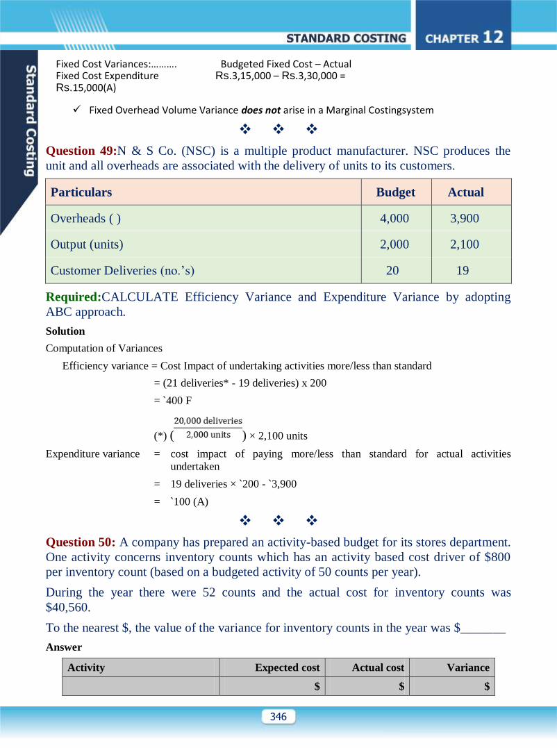
Question 49:N & S Co. (NSC) is a multiple product manufacturer. NSC produces the
unit and all overheads are associated with the delivery of units to its customers.
Particulars Budget Actual
Overheads ( ) 4,000 3,900
Output (units) 2,000 2,100
Customer Deliveries (no.’s) 20 19
Required:CALCULATE Efficiency Variance and Expenditure Variance by adopting
ABC approach.
Solution
Computation of Variances
Efficiency variance = Cost Impact of undertaking activities more/less than standard
= (21 deliveries* - 19 deliveries) x 200
= `400 F
(*) ( ) × 2,100 units
Expenditure variance = cost impact of paying more/less than standard for actual activities
undertaken
= 19 deliveries × `200 - `3,900
= `100 (A)
Question 50: A company has prepared an activity-based budget for its stores department.
One activity concerns inventory counts which has an activity based cost driver of $800
per inventory count (based on a budgeted activity of 50 counts per year).
During the year there were 52 counts and the actual cost for inventory counts was
$40,560.
To the nearest $, the value of the variance for inventory counts in the year was $_______
Answer
Activity Expected cost Actual cost Variance
$ $ $
Page 55
347
Inventory counts (based on 52
counts)
41,600 40,560 1,040 (F)
Question 51: XX produces the Unit and all overheads are associated with the delivery of
units to its customers. Budget details for the period include $8,000 overheads, 4000 units
output and 40 customer deliveries. Actual results for the period are $7,800 overheads,
4,200 units output and 38 customer deliveries. Calculate overhead volume and exp
variance.
Answer: the overhead cost variance for the period is
$
Actual cost 7,800
Standard cost (4,200 units × $2 per unit) 8,400
Cost variance 600 (F)
Applying the traditional fixed overhead cost variance analysis gives the following result:
$
Volume variance ($8,400 standard - $8,000 budget) 400 F
Expenditure variance ($8,000 buget - $7,800 actual) 200 F
Cost variance 600 F
Adopting an ABC approach gives the following result:
$
Efficiency variance (42 standard – 38 actual deliveries) × $200 800 F
Expenditure variance [(38 deliveries x $200)] - $7,800 200 A
Cost variance 600 F
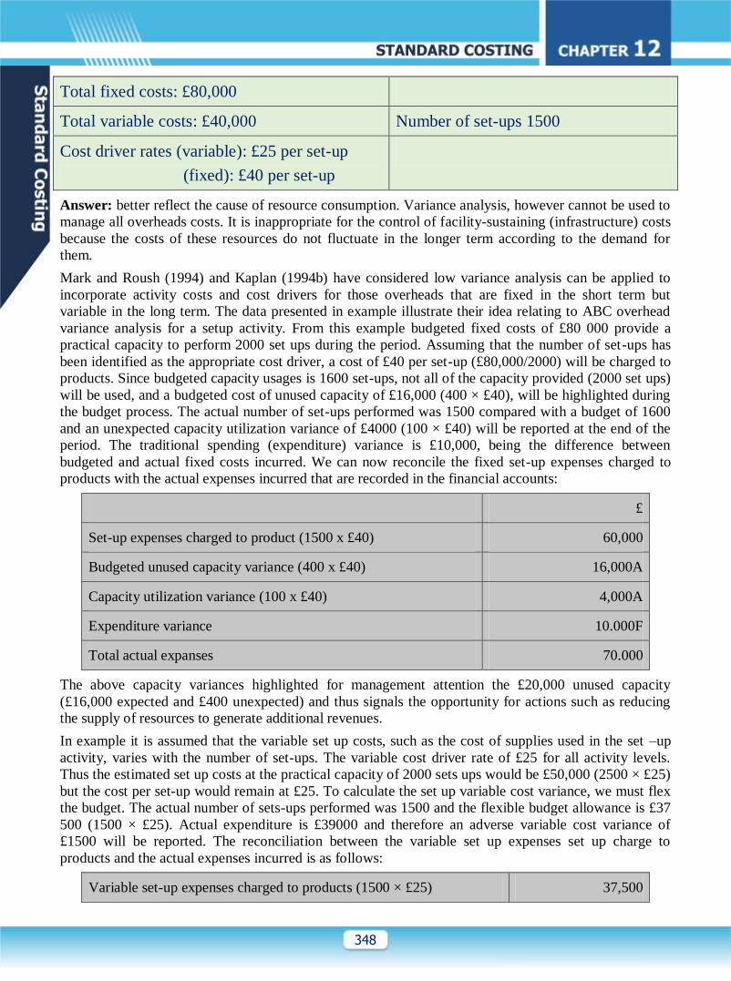
Question 52: Assume the following information for the set-up activity for a period:
Budget Actual
Activity level: 1600 set-ups Total fixed costs: £70,000
Practical capacity supplied: 2000 set-ups Total variable costs: £39,000
Page 56
348
Total fixed costs: £80,000
Total variable costs: £40,000 Number of set-ups 1500
Cost driver rates (variable): £25 per set-up
(fixed): £40 per set-up
Answer: better reflect the cause of resource consumption. Variance analysis, however cannot be used to
manage all overheads costs. It is inappropriate for the control of facility-sustaining (infrastructure) costs
because the costs of these resources do not fluctuate in the longer term according to the demand for
them.
Mark and Roush (1994) and Kaplan (1994b) have considered low variance analysis can be applied to
incorporate activity costs and cost drivers for those overheads that are fixed in the short term but
variable in the long term. The data presented in example illustrate their idea relating to ABC overhead
variance analysis for a setup activity. From this example budgeted fixed costs of £80 000 provide a
practical capacity to perform 2000 set ups during the period. Assuming that the number of set-ups has
been identified as the appropriate cost driver, a cost of £40 per set-up (£80,000/2000) will be charged to
products. Since budgeted capacity usages is 1600 set-ups, not all of the capacity provided (2000 set ups)
will be used, and a budgeted cost of unused capacity of £16,000 (400 × £40), will be highlighted during
the budget process. The actual number of set-ups performed was 1500 compared with a budget of 1600
and an unexpected capacity utilization variance of £4000 (100 × £40) will be reported at the end of the
period. The traditional spending (expenditure) variance is £10,000, being the difference between
budgeted and actual fixed costs incurred. We can now reconcile the fixed set-up expenses charged to
products with the actual expenses incurred that are recorded in the financial accounts:
£
Set-up expenses charged to product (1500 x £40) 60,000
Budgeted unused capacity variance (400 x £40) 16,000A
Capacity utilization variance (100 x £40) 4,000A
Expenditure variance 10.000F
Total actual expanses 70.000
The above capacity variances highlighted for management attention the £20,000 unused capacity
(£16,000 expected and £400 unexpected) and thus signals the opportunity for actions such as reducing
the supply of resources to generate additional revenues.
In example it is assumed that the variable set up costs, such as the cost of supplies used in the set –up
activity, varies with the number of set-ups. The variable cost driver rate of £25 for all activity levels.
Thus the estimated set up costs at the practical capacity of 2000 sets ups would be £50,000 (2500 × £25)
but the cost per set-up would remain at £25. To calculate the set up variable cost variance, we must flex
the budget. The actual number of sets-ups performed was 1500 and the flexible budget allowance is £37
500 (1500 × £25). Actual expenditure is £39000 and therefore an adverse variable cost variance of
£1500 will be reported. The reconciliation between the variable set up expenses set up charge to
products and the actual expenses incurred is as follows:
Variable set-up expenses charged to products (1500 × £25) 37,500
Page 57
349
Variable overhead variance 1,500 A
Total actual expenses 39,000
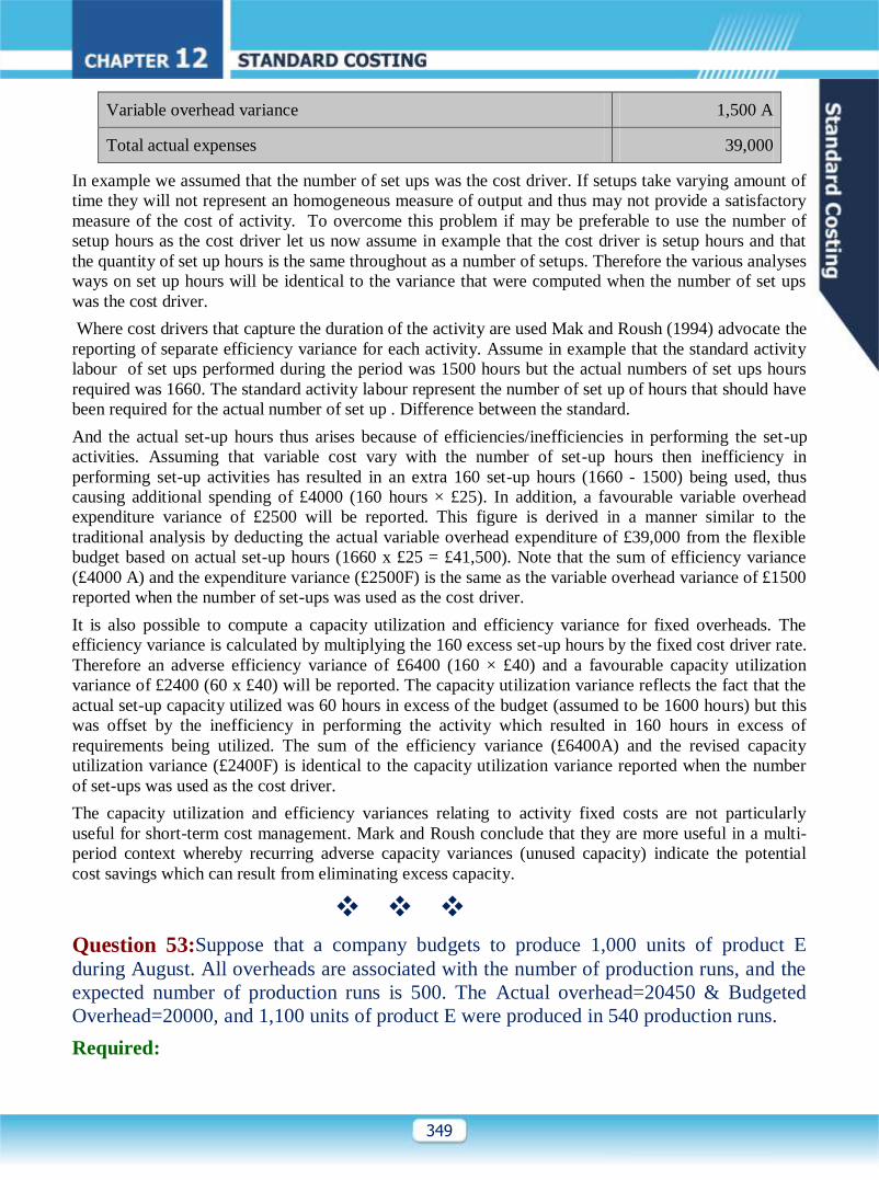
In example we assumed that the number of set ups was the cost driver. If setups take varying amount of
time they will not represent an homogeneous measure of output and thus may not provide a satisfactory
measure of the cost of activity. To overcome this problem if may be preferable to use the number of
setup hours as the cost driver let us now assume in example that the cost driver is setup hours and that
the quantity of set up hours is the same throughout as a number of setups. Therefore the various analyses
ways on set up hours will be identical to the variance that were computed when the number of set ups
was the cost driver.
Where cost drivers that capture the duration of the activity are used Mak and Roush (1994) advocate the
reporting of separate efficiency variance for each activity. Assume in example that the standard activity
labour of set ups performed during the period was 1500 hours but the actual numbers of set ups hours
required was 1660. The standard activity labour represent the number of set up of hours that should have
been required for the actual number of set up . Difference between the standard.
And the actual set-up hours thus arises because of efficiencies/inefficiencies in performing the set-up
activities. Assuming that variable cost vary with the number of set-up hours then inefficiency in
performing set-up activities has resulted in an extra 160 set-up hours (1660 - 1500) being used, thus
causing additional spending of £4000 (160 hours × £25). In addition, a favourable variable overhead
expenditure variance of £2500 will be reported. This figure is derived in a manner similar to the
traditional analysis by deducting the actual variable overhead expenditure of £39,000 from the flexible
budget based on actual set-up hours (1660 x £25 = £41,500). Note that the sum of efficiency variance
(£4000 A) and the expenditure variance (£2500F) is the same as the variable overhead variance of £1500
reported when the number of set-ups was used as the cost driver.
It is also possible to compute a capacity utilization and efficiency variance for fixed overheads. The
efficiency variance is calculated by multiplying the 160 excess set-up hours by the fixed cost driver rate.
Therefore an adverse efficiency variance of £6400 (160 × £40) and a favourable capacity utilization
variance of £2400 (60 x £40) will be reported. The capacity utilization variance reflects the fact that the
actual set-up capacity utilized was 60 hours in excess of the budget (assumed to be 1600 hours) but this
was offset by the inefficiency in performing the activity which resulted in 160 hours in excess of
requirements being utilized. The sum of the efficiency variance (£6400A) and the revised capacity
utilization variance (£2400F) is identical to the capacity utilization variance reported when the number
of set-ups was used as the cost driver.
The capacity utilization and efficiency variances relating to activity fixed costs are not particularly
useful for short-term cost management. Mark and Roush conclude that they are more useful in a multi-
period context whereby recurring adverse capacity variances (unused capacity) indicate the potential
cost savings which can result from eliminating excess capacity.
Question 53:Suppose that a company budgets to produce 1,000 units of product E
during August. All overheads are associated with the number of production runs, and the
expected number of production runs is 500. The Actual overhead=20450 & Budgeted
Overhead=20000, and 1,100 units of product E were produced in 540 production runs.
Required:
Page 58
350
Calculate the fixed overhead total variance and its sub-variance adopting the traditional
approach and then calculate the efficiency and expenditure variances using a ABC
approach.
Solution:
Applying the traditional fixed overhead cost variance analysis gives the following results.
A: Fixed overhead total variance
$
Fixed overhead incurred 20,450
Standard Cost (1,100 units X ($20,000/ 22,000
Fixed overhead total variance 1,550 (F)
(a) Fixed overhead expenditure varicne
$
Budgeted fixed overhead expenditure 20,000
Actual Fixed overhead expenditure 20,450
Fixed overhead Expenditure variance 450(A)
Fixed overhead volume variance
$
Actual production at Standard rate (1,100 × $20 pe r unit) 22,000
Budgeted production at standard rate (1,00 × $20 per unit) 20,000
Fixed overhead volume variance 2,000 (F)
Adopting an ABC approach gives the following results.
The efficiency variance highlight the impact of undertaking more or lower activities (production runs)
than budget.
$
Number of production runs should have been (1,100 × 0.5 per unit) 550
540
10 (F)
X Standard cost per run ( $20,000/500) 40
Efficiency Variance 400 (F)
The expenditure variance highlights the effect of paying more or less than budget for the actual number
of activities (production runs) undertaken.
Page 59
351
$
540 production runs should have cost (X $40 per run) 21,600
But dis cost 20,450
Expenditure variance 1,150 (F)
Question 54: Toymaster Ltd. Produces a plastic toy car, TGC in batches. To manufacture
a batch of TGCs, Toymaster must setup the machines. Setup costs are batch-level costs.
A separate setup Department is responsible for setting up machines for TGC.
Setup overhead costs consist of some costs that are variable and some that are fixed with
respect to the number of setup-hours. The following information pertains to 2007:
Static budget
amounts
Actual amounts
Units of TGC produced and sold 30,000 22,500
Batch size (number of units per batch) 250 225
Setup-hours per batch 5 5.25
Variable overhead cost per setup-hour `250 `240
Total fixed setup overhead costs `1,80,000 `1,75,350
Required:—
1. For variable setup overhead costs, compute the efficiency and spending variances.
Comment on the results.
2. For fixed setup overhead costs, compute the spending and the production-volume
variance. Comment on the results.
Solution:
Activity based costing, variance analysis.
1.
Static budget amounts Actual amounts
(a) Units of TGC produced and sold 30,000 22,500
(b) Batch size 250 225
(c) Number of batches (a ÷ b) 120 100
(d) Setup-hours per batch 5 5.25
(e) Total setup-hours (c × d) 600 525
Page 60
352
Static budget amounts Actual amounts
(f) Variable overhead cost per setup-hour `250 `240
(g) Variable setup overhead costs (e × f) `1,50,000 `1,26,000
(h) Total fixed setup overhead costs `1,80,000 `1,75,350
(i) Fixed overhead cost per setup-hour (h ÷ e) `300 `334
The flexible –budget is based on the budgeted number of setups for the actual output achieved:
22,500 units ÷250 units per batch = 90 batches
Computation of variable overhead cost variances follows:
Actual costs incurred Actual input × budgeted rate Flexible budget: Budgeted
input allowed for actual
output × budgeted rate
(100 × 5.25 × `240)
`1,26,000
(100 × 5.25 × `250)
`1,31,250
(90 × 5.0 × `250)
`1,12,500
` 5,250 F `18,750 U
Price variance Efficiency variance
The favorable spending variance is due to the actual variable overhead cost per setup-hour declining
from the budgeted `250 per hour to the actual rate of `240 per hour. The unfavorable efficiency variance
is due to the actual output of 22,500 units (1) requiring more setup (100) than the budgeted amount (90),
and (2) each setup taking longer time (5.25 hours) than the budgeted time (5.0 hours). The flexible-
budget variance of `13,500 it reflects the larger unfavorable efficiency variance not being offset by the
favorable spending variance.
2. Computation of the fixed setup overhead cost variance follows:
Actual costs incurred Actual input X budgeted rate Flexible budget: Budgeted
input allowed for actual
output X budgeted rate
(100 × 5.25 × `240)
`1,26,000
(100 × 5.25 × `250)
`1,31,250
(90 × 5.0 × `250)
`1,12,500
` 5,250 F `18,750 U
Spending variance Production- volume variance
Question 57: Choc Co is a company which manufactures and sells three types of biscuit
in packets. One of them is called ‘Ooze’ and contains three types of sweetener: honey,
sugar and syrup. The standard materials usage and cost for one unit of Ooze (one packet)
is as follows:
$
Honey 20 grams at $0.02 per gram 0.40
Page 61
353
Sugar 15 grams at $0.03 per gram 0.45
syrup 10 grams at $0.025 per gram 0.25
1.10
In the three months ended 30 November, Choc Co, produced 101, 000 units of ‘Ooze’
using 2200 kg of honey, 1400 kg of sugar and 1050 kg of syrup. Note: there are 1000
grams in a kilogram (kg).
Choc Co has used activity based costing to allocate its overheads for a number of years.
One of its main overheads is machine set-up costs. In the three months ended 30
November the following information was available in relation to set-up costs:
Budget
Total no. of units produced 264,000
Total no. of set-ups 330
Total set-up costs $52,800
Actual
Total no. of units produced 320,000
Total no. of set-ups 360
Total set-up costs $60,000
Required:
(a) Calculate the following variances for materials in ooze:
(i) Total materials usage variance
(ii) Total materials mix variance;
(iii) Total materials quantity (yield) variance
(b) Calculate the following activity-based variance in relation to the set-up cost of the
machines:
(i) The expenditure variance;
(ii) The efficiency variance
Solution: (a) (i) usage variance
Std usage for
actual output
Actual usage Std cost Variance
kgs kgs variance Per kg $ $
Honey 2020 2200 (180) 20 (3600)
Sugar 1515 1400 115 30 3450
Syrup 1010 1050 (40) 25 (1000)
(1150)A
(ii ) Mix variance
Page 62
354
Std usage for
actual output
Actual usage Std cost Variance
kgs kgs variance Per kg $ $
Honey 2066.67 2200 (133.33) 20 (2666.60)
Sugar 1550 1400 150 30 4500
Syrup 1033.33 1050 (16.67) 25 (416.75)
(1416.65)F
(i) Yieldvariance Std usage for
actual output
Actual
usage
Std cost Variance
kgs kgs variance Per kg $ $
Honey 2020 2066.67 (46.67) 20 (933.40)
Sugar 1515 1550 (35) 30 (1050)
Syrup 1010 1033.33 (23.33) 25 (583.25)
(2566.65) The above usage and mix variance have been calculated following the approach described in section titled ‘Direct Materials mix and yield variances’. For the actual output of 101,000 units the standard usage for actual output is 2020 kg of sugar (101,000 x 20/1000), 1515 kg of sugar (101,000 x 10/1000). To calculate the mix variance, it is necessary to ascertain the standard mix for the actual total quantity of inputs used (4650 kg). the standard mix for one unit of output is 20 grams of honey, 15 grams of sugar and 10 grams of syrup giving a standard mix of 20/45 honey, 15/45 sugar and 10/45 syrup. Therefore an actual input of (4650kg x 20/25), 1550kg of sugar (4650 x 15/45) and 1033 kg of syrup (4650 x 10/45).
The yield variance is calculated in a different way to the approach described in chapter 18. For the actual output (101,000 units), the standard quantities in the standard input mix are determined. They are compared with the actual quantities of inputs used based on the standard mix and the differences are multiplied by the standard input prices. This approach neutralizes the impact of the mix variance. For an actual input of 4650 kg an output of 103,333 units should result (4650kg/45 grams per unit of output). Therefore output was 2333 units fewer than it should have been for the input. This shortfall is multiplied by the standard cost of one unit of output ($1.10) giving an adverse variance of$2566.
(b ) (i) expenditure variance
Cost driver rate = $52,800/330 = $160 Expected cost = 360x$160 $57,600 Actualcost $60,000 Variance $2,400A
(ii) Efficiencyvariance
Expected no. of units per set up 264,000/330 = 800
Expected no. of set-ups for
320,000 =320,000/800= 400
Actual no. ofset ups 360
Difference 40F
X standard rateperset-up $160
Variance $6400F.
Page 63
355
STANDARD COSTING WITH LEARNING CURVE
Question 58: A company needs to calculate a new standard cost for one of its products.
When the product was first manufactured, the standard variable cost of the first unit was
as follows.
Cost per unit
$
Direct material 10 kg @ $4 per kg 40
Direct labour 10 hours @ $9 per hour 90
Variable overhead 10 hours @$1 per hour 10
Total 140
During the following year, a 90% learning curve was observed in making the product.
The cumulative production at the end of the third quarter was 50 units. After producing
50 units, the learning effect ended and all the subsequent units look the same time to
make.
Required:What is the standard cost per unit for the fourth quarter assuming the learning
curve had reached a steady state is peak efficiency was reached after the 50th unit was
produced?
Solution
where b = log0.9/log2.
b = - 0.0457575/0.30103 = -0.1520031
For 49 cumulative units Y = 10 × (49-0.1520031) = 10 × 0.55346 hours = 5.5346 hours.
Total time for first 49 units = 49 × 5.5346 hours = 271.2 hours.
For 50 cumulative units Y = 10 × (50-0.1520031) = 10 × 0.55176 hours = 5.5176 hours.
Total time for first 50 units = 50 × 5.5176 hours 271.2 hours = 275.88 hours.
Time for 50th unit = (275.88 – 271.2) = 4.68 hours
This is the standard time for the product when the steady state has been reached.
Standard cost Cost per unit
$
Direct material 10 kg @ $4 per kg 40.00
Direct labour 4.68 hours @ $9 per hour 42.12
Variable overhead 4.68 hours @$1 per hour 4.68
Page 64
356
Total 86.80
In practice, the standard time may be rounded to a more convenient number, such as 4.5 hours or 5.0
hours.
Question 59: City International Co. is a multiproduct firm and operates standard costing
and budgetary control system. During the month of June firm launched a new product.
An extract from performance report prepared by Sr. Accountant is as follows:
Particulars Budget Actual
Output 30 units 25 units
Direct Labour Hours 180.74 hrs. 118.08 hrs.
Direct Labour Cost `1,19,288 ` 79,704
Sr. Accountant prepared performance report for new product on certain assumptions but
later on he realized that this new product has similarities with other existing product of
the company.
Accordingly, the rate of learning should be 80% and that the learning would cease after
15 units.
Other budget assumptions for the new product remain valid.
The original budget figures are based on the assumption that the labour has learning rate
of 90% and learning will cease after 20 units, and thereafter the time per unit will be the
same as the time of the final unit during the learning period, i.e. the 20th unit. The time
taken for 1st unit is 10 hours.
Required:Show the variances that reconcile the actual labour figures with revised
budgeted figures in as much detail as possible.
Note:The learning index values for a 90% and a 80% learning curve are −0.152 and
−0.322 respectively.
[log 2 = 0.3010, log 3 = 0.47712, log 5 = 0.69897, log 7 = 0.8451, antilog of 0.6213 =
4.181, antilog of 0.63096 = 4.275]
Solution:
Working Note
The usual learning curve model is
y = axb
Where,
y = average time per unit for x units
a = Time required for first unit
x = cumulative number of units produced
b = learning coefficient
Page 65
357
W.N.1
Time required for first 15 units based on revised learning curve of 80% (when the time required for the
first unit is 10 hours)
y = 10 x (15)-0.322
log y = log 10 – 0.322 × log 15
log y = log 10 – 0.322 × log (5 x 3)
log y = log 10 – 0.322 × [log5 + log3]
log y = 1 – 0.322 × [0.69897 + 0.47712]
log y = 0.6213
y = antilog of 0.6213
y = 4.181 hours
Total time for 15 units = 15 units × 4.181 hours
= 62.72 hours
Time required for first 14 units based on revised learning curve of 80% (when the time required for the
first unit is 10 hours)
y = 10 × (14)-0.322
log y = log 10 – 0.322 × log 14
log y = log 10 – 0.322 × log (2 x 7)
log y = log 10 – 0.322 × [log2 + log7]
log y = 1 – 0.322 x [0.3010 + 0.8451]
log y = 0.63096
y = antilog of 0.63096
y = 4.275 hours
Total time for 14 units = 14 units × 4.275 hours
= 59.85 hours
Time required for 25 units based on revised learning curve of 80% (when the time required for the first
unit is 10 hours) total time for first 15 units = 62.72 hrs
Total time for next 10 units = 28.70 hrs [(62.72 – 59.85) hours × 10 units]
Total time for 25 units = 62.72 hrs + 28.70 hrs
= 91.42 hrs
W.N.2
Computation of Standard and Actual Rate
Standard Rate = = `660.00 per hr.
Actual rate = = `675.00 per hr.
W.N.3
Computation of Variances
Page 66
358
Labour rate variance = actual hrs × (std. rate – actual rate)
= 118.08 hrs × (`660.00 - `675.00)
= `1,771.20 (A)
Labour efficiency variance = std. rate × (std hrs – actual hrs)
= `660 × (91.42 hrs – 118.08 hrs)
= `17,595.60 (A)
Statement of Reconciliation (Actual Figures Vs Budgeted Figures)
Particulars `
Actual Cost 79,704.00
Less: Labour Rate Variance (Adverse) 1,771.20
Less: Labour Efficiency Variance (Adverse) 17,595.60
Budgeted Labour Cost (Revised)* 60,337.20
Budgeted labour cost (revised)*
= Std. Hrs. × Std. Rate
= 91,42 hrs. × `660
= `60,337.20
Question 60: The direct labour efficiency variance in respect of a new product has been
calculated as $14,700 favorable. The variance was calculated using standard cost data
which showed that each unit of the product was expected to take 8 hours to produce, at a
cost of $15 per hour.
The actual output was 560 units, and the actual time worked in the manufacture of the
product totaled 3,500 hours, at a cost of $57,750. However, the production manager now
realizes that the standard time of 8 hours per unit was the time taken to produce the first
unit and that a learning curve rate of 90% should have been anticipated for the first 600
units.
Required:Calculate the planning and operational efficiency variance for labour
efficiency, following the recognition of the learning curve effect (b = -0.1520 for a 90%
learning curve).
Answer: The ‘8 hours’ original standard does not take into account the presence of a learning curve
effect, that affects the first 600 units. By the time we reach 560 units of production, we have been
average time per unit of 3.0574 hours:
Y = 8 hours x 560 units-0.1520
Y = 3.0574 hours an average per unit (revised standard).
Therefore the first 560 units should have taken:
8 hours per unit × 560 units = 4,480 hours using the original, old standard labour hours per unit, and
Page 67
359
3.0574 hours per unit × 560 units = 1,712 hours, using the revised standard labour hours per unit.
This is a favorable difference of 2,768 hours and therefore the planning variance for labour efficiency
may be calculated as 2,768 hours x $15 = $41,520 Favorable.
To calculate the operational variance, we compare the standard number of labour hours for actual
production (1,712 hours, using the revised standard) and the actual time of 3,5000 hours, giving 1,788
hours ADV × $15 = $26,820 ADV.
AH x SR 1,450 × $10 = $14,500
Operational variance $500 F
RSH x SR 1,500 × $10 = $15,000
Planning variance $2,500 A
SH x SR 1,250 × $10 = $12,500
$2,000 A
Question 61:Bokco is a manufacturing company. It has a small permanent workforce but
it is also reliant on temporary workers, whom it hires on three month contracts whenever
production requirements increase. All buying of material is the responsibility of the
company’s purchasing department and the company’s policy is to hold low levels of raw
materials in order to minimize inventory holding costs. Bokco uses cost plus pricing to
set the selling prices for its products ones an initial cost card has been drawn up. Prices
are then reviewed on a quarterly basis. Detailed variance reports are produced each
month for sales, material costs and labour costs. Departmental managers are then paid a
monthly bonus depending on the performance of their department.
One month ago, Bokco began production of a new product. The standard cost card for
one unit was drawn up to include a cost of $84 for labour., based on seven hours of
labour at $12 per hour. Actual output of the product during the first month of production
was 460 units and the actual time taken to manufacture the product totaled 1,860 hours at
a total cost of $26,040.
After being presented with some initial variance calculations, the production manager has
realized that the standard time per unit of seven hours was the time taken to produce the
first unit and that a learning rate of 90% should have been anticipated for the first 1,000
units of production.
The production manager has been asked to recalculate the standard time for the first 460
units, based on a learning rate of 90%.
Note: the learning index b for a 90% learning curve is -0.1520.
1. What is the revised standard time for the first 460 units based on a learning rate of
90%.
A. 2,757 hours
B. 1,268 hours
Page 68
360
C. 2,898 hours
D. 3,220 hours
2. An engineer has now informed the production manger that the learning rate should
have been 85%. Based on this, he has correctly calculated that the revised standard
time for the first 460 units is 765 hours.
What are the labour efficiency planning and labour efficiency operational
variances?
Planning Operational
A $29,460 favorable $16,320 adverse
B $29,460 adverse $13,140 adverse
C $206,220 favorable $91,980 adverse
D $29,460 favorable $13,140 adverse
3. The following reasons were given by the engineer for changing the expected
learning rate from 90% to 85%:
(1) Staff turnover was lower than expected
(2) Unexpected problems were encountered with production
(3) Unexpected changes to Health and safety laws meant that the company had to
increase the number of breaks for employees during production
Which reasons could have caused the difference between the original and
revised rate of learning?
(a) 1, 2 and 3
(b) 2 and 3 only
(c) 1 only
(d) None of the statements
4. The production manger has been criticized by other departmental managers for
failing to take into account the learning rate in the original standard. They claim
“he has no idea of all the problems this has caused”.
Which of the following might have been caused by the failure of the production
manger to take into account the learning rate in the original standard?
(1) Insufficient numbers of temporary staff would have been employed, leading to
an inability to satisfy demand
(2) Since the company uses the cost plus pricing, the price for the product will have
been set too high leading to a fall in demand for the product
(3) The sales manager will be held responsible for the poorer sales of the product,
which will probably be reflected in an adverse sales volume variance. He will
become demotivated
(4) Since production is actually happening more quickly than anticipated, the
company may well have run out of raw materials, leading to a stop in
production.
A. 1, 2 and 4 only
B. 1 and 4 only
Page 69
361
C. 2,3 and 4
D. 2 and 3 only
5. Which of the following statements concerning planning and operational variance
are true?
(1) If the variance calculated using the original standard is adverse, then the
operational variance will always be adverse
(2) Operational variance are generally a better reflection of the underlying
performance of managers than traditional variances
(3) Planning variances reflect factors outside of the control of operational
managers.
(4) 1, 2 and 3
(5) 2 and 3 only
(6) 1 only
(7) None of the statements
Solution: Justification
1. B. Revised hours for actual production:
Cumulative time per hour for 460 units is calculated by using the learning curve formula:
Y = axb
a=7
x= 460
b =-0.1520
Therefore y=7 × 460 -0.1520 =2.7565054
Therefore revised time for 460 units = 1,268 hours (460 × 2.7565054).
2. D. Labour efficiency planning variance
(Standard hours for actual production- revised hours for actual production) × Standard rate
=([460 × 7] -765 ) × $12 = $29,460 F
Labour efficiency operational variance
(Revised hours for actual production – actual hours for actual production × standard rate (765 -
1,860) × $12 = $13,140A
3. C. The revised learning rate of 85% was actually better than the original expected rate of 90%
and only (i) Cold cause it to improve.
4. C. (1) is incorrect. Bokco will have hired too many temporary staff because of the fact that the
new product can actually be produced more quickly than originally thought.
(2) Is correct. The budgeted cost, on which the price is based would be too high since it does not
take account of the labour efficiencies as a result of the learning.
(3) Since the price charged is too high (Statement 2), demand for the product will fall.
(4) Production will occur more quickly since the time per unit is less than anticipated.
5. B. The Operational variance shows the difference between the revised standard and the actual
performance. This could be adverse or favorable, even if the variance calculated using the
original standard is adverse, so (1) is incorrect. The other two statements are correct.
Question 63:Martin Co developed a new product. it set a standard labour cost based on
the expected time to make the first unit of the product, which has 100 minutes. A 90%
Page 70
362
learning rate is expected to apply, and the budgeted cost per hour of labour time is $12
per hour. This learning rate was not incorporated into the standard.
The actual time taken to make the first four units was 350 minutes and the cost was $80.
Required:
(a) Calculate traditional labour rate and efficiency variances.
(b) Re-calculate the labour efficiency variance to take account of the learning rate.
Solution:
(a) labour rate variance
$
actual labour hours × actual rate 80
Actual labour hours × standard rate (350/60) × $12 70
Labou rate variance (adverse) 10
Labour efficiency variance
$
actual labour hours × standard rate 70
standard hours for actual production x standard rate (working) 324
minutes × $12/60
65
Labour efficiency variance (adverse) 5
Working – standard hours for actual production taking into account the learning rate of 90%.
Output
(units)
Cumulative average time Total time
1 100 100
2 90 180
4 81 324
Question 65:S uses a standard absorption costing system to control its production costs
and monitors its performance using monthly variance reports.
S has recently launched a new product which is being manufactured in batches of 100
units. An extract from the standard cost details per unit for this new product is as follows:
5.3 hours of direct labour @ $10 per hour = $53.00
It is now realized that the standard cost details were based on an average learning period
target of 5.3 hours per unit, and that a batch related period of learning was expected. The
time expected for the initial batch was 1,000 hours and 90% learning rate was anticipated.
Page 71
363
During August production commenced on the product, and 400 units were produced in
four batches of 100 units using 2500 hours of direct labour at a cost of $26,000. The
direct labour variances that were reported in respect of this product were:
Direct labour rate variance $1,000 Adverse
Direct labour efficiency variance $3,800 Adverse
Required:
(a) Calculate the expected length of the learning period in batches.
(b) Calculate planning and operating variances for August. Answer: (a)
No. of batches completed Average time per batch
1 1,000 hours
2 900 hours
4 810 hours
8 729 hours
16 656 hours
32 590 hours
64 531 hours
Note: with a 90% learning rate, the cumulative average time per unit of output will fall to 90% of what
it was before, every time output is doubled.
Expected length of learning period = 64 batches
(average time of 5.3 hours per unit; 530 hours per batch of 100 after 64 batches have been completed).
(b) S produced 4 batches of the new product in August. The average time per batch should have been
810 hours
4 batches should have taken (4 × 810 hours) 3,240 hours
4 batches did take 2,500 hours
740 hours (F)
Standard rate $10/hr
Operating efficiency variance $7,400 (F)
The planning variance is calculated by comparing the standard target time with the revised target time:
Original standard (5.3 hrs × 400 units) 2,120 hours
Revised standard (4 x 810 hrs) 3,240 hours
1,120 hours (A)
Standard rate $10/hr
Page 72
364
Planning efficiency variance $11,200 (A)
RECONCILATION
Question 66: Queensland Chemicals (QC) manufactures high-quality chemicals C-1, C-2
and C - 3. Extracts from the budget for last year are given below:
C-1 C-2 C-3
Sales Quantity (kg) 1,000 3,250 750
/ kg / kg / kg
Average Selling Price 17,600 2,560 22,400
Direct Material (C2H6O) Cost 8,000 1,280 9,600
Direct Labour Cost 3,200 480 4,800
Variable Overhead Cost 320 48 480
The budgeted direct labour cost per hour was 160.
Actual results for last year were as follows:
C-1 C-2 C-3
Sales Quantity (units) 900 3,875 975
/kg /kg /kg
Average Selling Price 19,200 2,480 20,000
Direct Material(C2H6O) Cost 8,800 1,200 10,400
Direct Labour Cost 3,600 480 4,800
Variable Overhead Cost 480 64 640
The actual direct labour cost per hour was 150. Actual variable overhead cost per direct
labour hour was 20. QC follows just in time system for purchasing and production and
does not hold any inventory.
Required: INTERPRET the Sales Mix Variance and Sales Quantity variance in terms of
contribution.
Solution:-
Variance Interpretation
The sales quantity variance and the sales mix variance describe how the sales volume contribution
variance has been affected by a change in the total quantity of sales and a change in the relative mix of
products sold.
From the figures arrived for the sales quantity contribution variance, we can observe that the increase in
Page 73
365
total quantity sold would have gained an additional contribution of 2,124,600, if the actual sales volume
had been in the budgeted sales proportion.
The sales mix contribution variance shows that the variation in the sales mix resulted in a curtailment in
profit by 570,600. The change in the sales mix has resulted in a relatively higher proportion of sales of
C-2 which is the chemical that earns the lowest contribution and a lower proportion of C-1 which earn a
contribution significantly higher. The relative increase in the sale of C-3 however, which has the highest
unit contribution, has partially offset the switch in mix to C-2.
Workings
Statement Showing Standard Contribution
C-1
₹/ kg
C-2
₹/ kg
C-3
₹/ kg
Average Selling Price 17,600 2,560 22,400
Direct Material (C2H6O) Cost 8,000 1,280 9,600
Direct Labour Cost 3,200 480 4,800
Variable Overhead Cost 320 48 480
Contribution 6,080 752 7,520
Sales contribution mix variance
Products Actual
Quantity
[AQ]
Actual Sales at
Budgeted
Proportion [RAQ]
Difference
[AQ – RAQ]
Contribution
[SC]
Mix Variance
( ’ 000)
SC × [AQ – RAQ]
C-1 900 1,150 250 (A) 6,080 1,520 (A)
C-2 3,875 3,737.50 137.50 (F) 752 103.40 (F)
C-3 975 862.50 112.50 (F) 7,520 846 (F)
5,750 5,750 570.60 (A)
Sales contribution quantity variance
Products Budget
Sales
Quantity
[BQ]
Actual Sales at
Budgeted
Proportion
[RAQ]
Difference
[RAQ]
Contribution
[SC]
Qty. Variance
( ’ 000) SC ×
[RAQ – BQ]
C-1 1,000 1,150 150 (F) 6,080 912 (F)
C-2 3,250 3,737.50 487.50 (F) 752 366.60 (F)
C-3 750 862.50 112.50 (F) 7,520 846 (F)
5,000 5,750 2,124.60 (F)
Case Scenario
Page 74
366
Question 67: Natural Spices manufactures and distributes high-quality spices to gourmet
food shops and top quality restaurants. Gourmet and high-end restaurants pride
themselves on using the freshest,highest-quality ingredients.
Natural Spices has set up five state of the art plants for meeting the ever- growing
demand. The firm procures raw material directly from the centers of produce to maintain
uniform taste and quality. The raw material is first cleaned, dried and tested with the help
of special machines. It is then carefully grounded into the finished product passing
through various stages and packagedat the firm’s ultraclean factory before being
dispatched to customers.
The following variances pertain to last week of operations, arose as a consequence
ofmanagement’s decision to lower prices to increase volume.
Sales Volume Variance 18,000 (F)
Sales Price Variance 14,000 (A)
Purchase Price Variance 10,000 (F)
Labour Efficiency Variance 11,200 (F)
Fixed Cost Expenditure Variance 4,400 (F)
Required:
(i) Identify the ‘Critical Success Factors’ for Natural Spices.
(ii) Evaluate the management’s decision with the “Overall Corporate Strategy” and
“critical Success Factors”.
Solution:-
(i) Gourmet and high-end restaurants recognizes Natuarl spices on the basis of high quality of
spices. Therefore, quality is most critical success factor of Natural spices. There are other factors
which cannot be ignore such as price, delivery option, attractive packing etc. But all are
secondary to the quality.
(ii) Deliberate action of cutting price to increase sales volume indicates that firm is intending to
expand its market to retail market and street shops which is price sensitive.
Purchase Price Variance is clearly indicating that firm has purchased raw material at lower price which
may be due to buying of lower quality of material. Similarly, positive Efficiency Variance is indicating
cost cutting and stretching resources.
It appears that firm is intending to expand its market to retail market and street shops by not only
reducing the price but also compromising its quality which is opposing its current strategy of high
quality.
Management should monitor the trends of variances on regular basis and take appropriate action in case
of evidence of permanent decline in quality. Here, customer feedback is also very important.
Question 68: A company manufactures two types of fertilizers (FA and FB). The
company uses a standard costing system for planning and control purposes. Standards are
set annually but budgets and variance reports are prepared each period.
Page 75
367
Chemicals
Three chemicals (C1, C2 and C3) are used to make the fertilizers. C2 and C3 can be input
directly to the manufacturing process but C1 has to be treated before it can be used. The
treatment results in a loss of 30% of the chemicals treated. There are no further losses in
the manufacturing process.
Details of the standards for the chemicals are as follows:
C1 C2 C3
Price per kg $8 $15 $12
Treatment loss 30%
Content of finished product:
Per unit of FA 0.20 kg 0.15 kg NIL
Per unit of FB 0.20 kg NIL 0.25kg
Inventory policies
Chemicals: end of period holdings must be equal to 50% of the following period’s
requirements.
Treated C1 is used immediately. There are never any inventories of treated C1 at the start
or end of any period.
Fertilizers: no finished products are to be held.
Period 1: output and sales
Budgeted units Actual units
FA 40,000 38,000
FB 24,000 25,000
Period 2 and 3: sales budgets
Budgeted units Actual units
FA 40,000 44,000
FB 24,000 33,000
Required:-
(a) During period 1, the quantity of C1 used was 17,740 kg. Calculate for period 1 for
C1:
(i) the materials usages variance for the whole process
(ii) the treatment loss percentage
(b) In period 1, the company purchased and used 6,450 kg of C3. The cost of this
purchase was $94,000. It has now been realized that the standard price of C3
should have been $14.50 per kg for period 1.
Page 76
368
Calculate the planning variance, and the operational price and usages variance for
C3 for period 1.
Solution:
(a) (i) FA 38,000 units should have used (0.2 kg/70%) 10,857.14
FB 25,000 units should have used (0.2 kg/70%) 7,142.86
But did use 17,740.00
Variance in kg 260.00 (F)
X standard cost per kg x $8
$2,080 (F)
(ii) content of output = (38,000 + 25,000) x 0.2 kg of x C1 = 12,600 kg of C1
Materials input = 17,740 kg of C1
Therefore, actual losses = 5,140 kg of C1
Therefore, actual loss percentage =
(b) Planning variance
$
Revised standard cost (25,000 units × 0.25 kg × $14.50) 90,625
Original standard cost (25,000 units × 0.25 kg × $12) 75,000
15,625(A)
Operational price variance
$
6,450 should have cost (x $14.50) 93,525
But did cost 94,000
475 (A)
Operational usages variance
25,000 units should have used (x 0.25kg) 6,250
But did use 6,450
Variance in kg 200 (A)
X revised standard cost per kg x $14.50
Standard with service sector
Question 69: Flexed budget for the cost of medical supplies in a hospital, based on a
percentage of maximum bed occupancy, are shown below:
Bed occupancy 82% 94%
Medical supplies cost $410,000 $429,200
During the period, the actual bed occupancy was 87% and the total cost of the medical
supplies was $430,000.
Identify the medical supplies expenditure variance:
A. $5,000 adverse
Page 77
369
B. $12,0000 adverse
C. $5,000 favorable
D. $12,000 favorable
Solution
Contribution margin
=
= $1,600 for every 1% chance
Budget for 87% occupancy = $429,200 – (7 x 1600)
= $418,000
Medical expenditure variance = 418,000 – 430,000
= $12,000 Adverse
Question 70:Secure Net (SN) manufactures security cards that restrict access to
government owned building around the world.
The standard cost for the plastic was $5.25 per kg and the production manager (who is
responsible for all buying and production issues) was asked to explain the increase. He
said ‘World oil price increases pushed up plastic prices by 20% compared to our budget
and I also decided to use a different supplier who promised better quality and increased
reliability for a slightly higher price. I know we have overspent but not all the increase in
plastic prices in my fault. The actual usage of plastic per card was 35 g per card and again
the production manager had an explanation. He said ‘the world-wide standard size for
security cards increased by 5% due to a change in the card reader technology, however,
our new supplier provided much better quality of plastic and this helped to cut down on
the waste’.
SN operates a just in time (JIT) system and hence carries very little inventory.
Required:
(a) Discuss the behavioral problems that can arise from using standard costs and ways
to prevent them.
(b) Analyse the above total variances into components parts for planning and
operational variances in as much detail as the information allows.
(c) Assess the performance of the production manager.
Solution: (a) behavioral problems that may arise from using standard costs
Standard costing is principally used to value inventories, to prepare budgets and to act as a control
device. The focus in using a standard cost system should not be to attribute blame, but to influence
behavior through positive support and appropriate motivation.
The perception of a standard costing system can affect its success or failure. A negative perception is
often the consequence of unreasonable standards, lack of transparency in setting standards, poor
Page 78
370
communication or uneven reward systems. Such situation can make a good standard cost system a
failure.
Ways to reduce negative perception/motivation
Organization should set understable and achievable standard, otherwise it neither motivates nor rewards
employees. Complex financial measures and reports mean nothing to most employees.
Employees should be involved in setting standards and developing performance measures. This should
result in realistic targets and increase employee motivation.
Standards should be well defined and communicated to all employees so that operational efficiency can
be achieved. Management should ensure that any performance-related scheme does not reward behavior
that goes against the best interest of the organization.
Finally, performance pay plans should be reviewed and update on a regular basis to meet the changing
needs of employees and the business as a whole.
(b) Total material planning variance
$
Original flexed budget cost (100,000 × $4 × 0.04kgs) 16,000
Revised flexed budget cost (100,000 × $4.80 × 0.042kgs) 20,160
4,160(A)
Planning price variance
Actual units × revised standard usage × (original standard price – revised standard price)
= 100,000 units × 0.042kgs × ($4.00 - $4.80) = $3,360 (A)
Planning usage variance
Actual units × original standard price × (original standard usage – revised standard usage)’
= 100,000 units × $4.00 × (0.04 kgs – 0.042 kgs) = $800 (A)
Planning price variance + planning usage variance = toattl planning variance
$3,360 + $800 = $4,160 (A)
Total material operational variance
$
Actual cost (for 100,000 units) 18,375
Revised standard cost (for 100,000 units) (0.042 kgs × $4.80) 20,160
Total operational variance 1,785 (F)
Operational price variance
$
Actual price of actual material (3,500 kg) 18,375
Revised standard price of actual materials ($4.80 × 3500 kg) 16,800
Operational price variance 1,575 (A)
Operational usage variance
Page 79
371
Actaula quantity should have benn 4,200 kgs
But was 3,500kgs
Operational usage variance in kgs 700 kgs (F)
X revised standard cost per kg X $4.80
Operational usage variance in $ $3,360 (F)
(c) world wide standard size
The size of the security card has to fit the reader of that card and if the industry specification changes
there is nothing that the production manager can do about it. This is beyond his control and therefore a
planning error and should not be used to assess his performance.
Oil prices
Worldwide oil prices have increased which have increased plastic prices and again the production
manager cannot control that. This is another planning error and should be ignored in an assessment of
his performance.
New supplier
The decision to use a new supplier cost an extra $1,575 which is the operational price variance and
could be regarded as poor performance by the production manager. However, the manager seems to
have agreed to the higher price on the promise of better quality and reliability.
The operational usage variance is $3,360 favorable and this could be as a result of improved quality.
Increase in production and sales
Production level increased significantly from 60,000 to 100,000 which could potentially has caused
problems for the production manger. However the ability to increase production suggests that the new
supplier’s reliability was good.
The total materials operational variance shows a favorable variance of $1,785 which reflects well on the
performance of the production manager. The ability to react and be flexible can often form a part of a
performance assessment.
In conclusion the manger could be said to have performed well.
Question71:A company using a detailed system of standard costing finds that the cost of
investigation or variances is `20,000. If after investigation an out of control situation is
discovered, the cost of corrective action is ` 30,000. If no investigation is made, the
present value of extra costs involved is `1,50,000.The probability of the process being in
control is 0.82 and the probability of the process being in control is 0.82 and the
probability of the process being out of control is 0.18
Advise(i) Whether Investigation of the variances should be undertaken or not (ii) the
probability at which it is desirable to institute investigation in to the variances.
Answer: This is a problem relating to the cost of administration of standard costing system.
Investigating into variances costs money, and taking corrective action, if necessary , also costs money .
If investigation and corrective actions are not carried out, the adverse variances will be a drain on the
profits. Hence it is necessary to strike a balance between the two.
Page 80
372
Action Costs it in control (`) Cost if out of control(`)
(a) If investigated 20,000 20,000 +30,000 = 50,000
(b) If not investigated 0 1,50,000
Expected value:
(i) (a) If investigated the probability of process beig in control is 0.82. Hence the expected value of
being in control is `20,000 × 0.82 = ` 16,400.
The probability of process being out of control is 0.18. Hence the expected value of being ou of
control is `50,000 × 0.18 = `9,000. So, the total cost of investigation is ` 16,400 + ` 9,000 = ` 25,400.
(b) If not investigated, the cost of continued incurrence of variances is `1,50,000 × 0.18 = `27,000.
Since the total costs are lower when investigation is done and corrective action is carried out, it is
advisable to investigate and take corrective action.
(ii) Put the probability of not investigating =p2. Then the probability of investigation = (1-p2).
Put, cost of investigation of `20,000 = C.
Cost of corrective action of ` 30,000 =M
Cost of variances of `1,50,000 = L
The cost indifference point is as follows:
Investigate = C (1-p2) + (C+M)p2 = Lp2
Solving the above equation, we get:
P2= C(L-M)
Substituting the data, we get:
` 20,000 (`1,50,000- `30,000) = 0.17
The conclusion is if the probability of the variances being in control is greater than 0.17,
investigation should be done. If it is less than 0.17, investigation should be done. If it is less than
0.17, investigation need not be done. At the probability value of 0.17, the company is indifferent to
undertaking the investigations.
Question 72: -Established in the year 1999, FF Company is the pioneer of fast
food in Southampton. It delivers a truly fresh, affordable, made to order
sandwiches, burger, and other meal in a friendly and relaxed environment. The
popularity of the sandwiches, burger etc. continuedto grow over the decades
but one thing remained the same and that was its core values andprinciples:
- Always provide exceptional service to valuedguests;
- Provide the highest quality menu items at a price everyone can afford
and enjoy;and
- Keep operating costs low and ensure to have great systems in
place and never stop improving.
It provides a comfortable place for people to unwind over interesting
conversations. From the beginning, as it continues to grow, it is guided by
Page 81
373
passion for delighting customers by serving fresh, delicious food right in front of
customer.
The performance report* for FY 2018-19 was presented at the management
committee meeting as follows:
Particulars Budget Actual Variance
Sales / Production (no. of burgers) 2,00,000 1,65,000 (35,000)
Sales (£) 10,50,000 8,46,450 (2,03,550)
Less: Variable Costs (£) 6,33,000 5,37,075 95,925
Less: Fixed Costs (£) 1,57,500 1,65,000 (7,500)
Profit 2,59,500 1,44,375 (1,15,125)
* burger segment
The Management Accountant of FF believed that the size of the fast-food
market deriving the budget number of burgers to be sold is over-estimated. He
has computedthe value of the sales volume contribution planning variance to
be 26,062.50adverse.
Further, the report also included customer’s feedback and the majority of
comments were regarding delay in service time. One of feedback was as follows:
“I ordered two burgers at 2:10 pm. After half an hour (30 minutes) of waiting I
called the waiter and asked him what happened? he told me that he will check
with kitchen. I gotthe order after 45 minutes of waiting, this cafe is not good in
deliverytime”
The budgeted data shown in the table is based on the assumption that total
market size would be 4,00,000 units.
Required
(i) PREPARE a reconciliation statement of budgeted profit to actual profit
through marginal costing approach in as much detail as possible.
(ii) EXPLAIN the implications of the reconciliation statement.
(iii) Management is worried about customer’s feedback. ADVISE measures to
improve delivery service time.
Solution:- Statement of Reconciliation:- Budgeted Vs Actual Profit
Particulars $
Budgeted Profit 2,59,500
Less: Sales volume contribution -Planning Variance
(Adverse)
26,062.50
Less: Sales Volume contribution-Operational Variance
(Adverse)
46,912.50
Less: Sales Price Variance (Adverse) 19,800
Less: Variable Cost Variance (Adverse) 14,850
Page 82
374
Less: Fixed Cost Variance (Adverse) 7,500
1,44,375
Workings
Basic Working
Budgets Market Share (in %) = %50
000,00,4
000,00,2
units
units
Budgeted Contribution = $ 10,50,000 - $ 6,33,000 = $ 4,17,000
Average Budgeted Contribution (Per unit)
= 085.2$
000,00,2
000,17,4$
Volume Contribution Planning = Budgeted Market Share % X (Actual industry Sales Quantity in units -
Budgeted Industry Sales Quantity in units) X (Average Budgeted Contribution per unit)
=$26,062.50(A) = 50% X (Actual Industry Sales Quantity in units - 4,00,000 units) X $2.085
= Actual Industy Sales Quantity = 3,75,000 units
Actual Market Share (In %) = %44000,75,3
450,46,8$
units=44%
Standard Sales Price per unit = 25.5$
000,00,2
000,50,10$
Actual Sales Price per unit = 13.5$
000,65,1
450,46,8$
Standard Variable Cost per unit = 165.3$
000,00,2
000,33,6$
Actual Variable Cost per unit = 255.3$
000,65,1
075,37,5$
CALCULATION OF VARIANCES
Sales Variance
Volume Contribution Operational = (Actual Market Share % -Budgeted Market Share %) X (Actual Industry
Sales Quantity in units) X ( Average Budgeted Contribution per unit)
= (44% - 50%) X 3,75,000 units X $ 2,085
= $ 46,912.50(A)
Price = Actual Sales -Standard Sales
= Actual Sales Quantity X (Actual Price -Standard Price)
= 1,65,000 units X( $5.13 - $ 5.25)
Page 83
375
= $19,800 (A)
Variable Cost Variance
Cost = Standard Cost for Production - Actual Cost
= Actual Production X (Standard Cost per unit -Actual
Cost per unit)
= 1,65,000 units X ( $ 3.165 - $ 3,255)
= $14,850 (A)
Fixed Cost variance
Expenditure = Budgeted Fixed Cost -Actual Fixed Cost
= $1,57,500 - $ 1,65,000
= $ 7,500 (A)
(iii) Implication of Reconcilitation Statement
(iv) In the revised statement the sales volume variance has been detailed by the way of two
variances I.e. planning and operational variances.THis kind of detailed information assists the company
to check , which kind of variances are under the management control and which are not. FF has
adverse volume contribution planning variance and the reason of could be the environmental/market
changes, that was not anticipated at the time of budget preparation, so they are not under
management control and hence, no one is responsible for this. On the other hand, the sales volume
contribution operational variance was under control of the managers and they should be held
responsible for the same.The reason of adverse sales volume contribution operational variance could
be unsuccessful direct selling efforts/marketing efforts.FF has adverse sales price variance as well. It
indicates that the budgets were sold for lower price than standard.The reason of this could be
unforeseen market competitive price, tapping new market etc.
Further revised reconciliation statement delivers little information about the variable cost and fixed cost
variances. They both are adverse, Fixed Cost consists of many items such as salaries, annual maintenance
cost, rent and insurance etc.Often fixed cost items are not affected in short run in response to change in
the level of activity , but they might change in response to other factors such as price.This may cause
increase expenditure on fixed overheads.A meaningful analysis of fixed cost variance requires a line to line
comparison of budgeted cost with actual cost.
In case of FF, the variable cost may be made up of large individual different items such as vegetables, gas,
indirect labor, regular maintenance cost etc. Control of variable cost also required line by line analysis for
each individual item. The adverse variable cost variance simply reveals that FF incurred more on variable
cost than expected. However it is necessary to take into consideration the causes of this adverse variacne
which is beyond the control of the management , for instance the unusual price hike in vegetables in case
of unseasonal rainfall.`
(iii) Measures to improve Fast Food Delivery Service Time
Customers expect that their food order to be delivered quickly. From customers feedback in the question,
it is evident that FF has a problem in food delivery , due to which , customers go unsatisfied.The reason of
late delivery could be non-availability of raw material on time or employees not working properly etc. The
reason of employees not working properly could be job dissatisfaction which may be due to improper
working conditions, low salary, or no reward for overtime etc.
In order to reduce delivery time, raw material should be made available in stock based on daily
requirement.FF may follow quantitative approach to inventory problems, which lay s down clear
guidelines that when to re-order or alert the management in exceptional situations.
In addition , FF must also address the issues related to employees and involve them in a loop. FF could
improve the employee satisfaction with proper working conditions, better pay, training and growth
opportunities.
Moreover, It is important that customers should be informed about approximate delivery time since this
Page 84
376
will reduce customers anxiety and will proactively reduce any complaints over long waits for delivery of
food. If unexpected delays occur, it is important to communicate with customers, apologies for the delay
and inform them about the new approximate delivery time along with valid reason.
In addition to this, FF can also introduce pages or install electronic board displaying ticket number or self-
serve kiosk allowing customers to roam around or order in advance so that they do not have long waiting
time.
SOLVED PROBLEMS
Market Size and Share
Question 73: Hudson has a sales budget of 400,000 units for the coming year based on
20% of the total market. On each unit, Hudson makes a profit of $3. Actual sales for the
year were 450,000, but industry reports showed that the total market volume had been 2.2
million.
(a) Find the traditional sales volume variance.
(b) Split this into planning and operational variances (market size and market share).
Comment on your results.
Answer: (a) Traditional Sale Volume variance
=(Actual units sold- Budgeted Sales) × Standard profit per unit
=(450,000 -400,000) × $3 = $15,000 F.
(b) Planning and operational variances The revised (ex-post) budget would
show that Hudson Ltd should expect to sell 20% of 2.2 million units
=440,000 units
Original Sales × Standard margin = 400,000 × $3 = $1,200,000
Market Size = $120,000 F
Revised Sales × Standard margin = 440,000 × $3 = $1,320,000
Market Share = $30,000 F
Actual Sales × standard margin =450,000 × $ 1,350,000
Total Sales volume variance = $12,000 F + $30,000 F = $150,000 F
Comment:
Most of the favorable variance can be attributed to the increase in overall
market size. However, some can be put down to effort by the sales force
which has increased its share from 20% to 20.5% (450,000/2,200,000)
Managers should only be appraised on the operational variance i.e. the
market share variance.
Question 74: A Company sets its sales budget based on an average price of $14 per unit
and sales volume of 250.000 units. Competition was more intense than expected and the
company only achieved sales of 220,000 and had to sell at a discounted price of $12.50
Page 85
377
per unit. The company was unable to reduce costs so profit per unit fell from $4 per unit.
The company was unable to reduce costs so profit per unit fell from $4 per unit to $2.50
per unit. It was estimated that the total market volume grew by 10% from 1,000,000 units
to 1,100,000 units.
Required:
(a) Calculate the sales price and volume variances.
(b) Analyse the volume variances into market share and market size.
(c) Discuss whether the price variances is a planning or operational variance.
Answer: (a) Sales price variance
= 220,000 × ($14 - $12.50) = $330,000A
Sales volume variance
= (250,000 -220,000) × $4 = $120,000 A
(b) Budgeted market share = 250,000/1,000,000 = 25%
The sales of 25% × 1,100,00 = 275,000 in the actual market conditions.
The market size variance
= (275,000 – 250,000) × $4 = $ 220,000 A
The increased market size is favorable as the company should sell more if
market share can be maintained. The market share variance was adverse as
market share fell from 25% to 220,000/1,100,000= 20%.
(c) It could be argued that the increased competition in the market was not
foreseen when the budget was set and the variance is thus a planning
variance. However , this line of reasoning would suggest that any unforeseen
issues give rise just to planning variances. Perheps sales managers should
have identified potential threats sooner? Also, once extra competition was
experienced , managers had to decide how to respond . This could have
involved additional advertising rather than price cuts. E.g. it could be argued
that price cuts were made to try (unsuccessfully) to protect market share, in
which case managers should be held (at least partly) responsible for such a
decision.
Question 75: The sale budget of Brunco was based on the following estimates:
Total size of market: 200,000 units
Expected market share: 25%
Standard contribution per unit $40
At the end of the year it was estimated that the actual size of the market during the
year has been 260,000 units.
Actual sales in the year were 61,000 units.
Required:
Page 86
378
Calculate for the year:
(a) The total sales volume variance
(b) The market size variance
(c) The market share variance.
Answer:
Units
Budgeted Sales volume (25% × 200,000) 50,000
Actual Sales volume 61,000
Sales volume variance in units 11,000 (F)
Standard contribution per unit X$40
Sales volume variance in $ contribution $440,000 (F)
Market size variance Units
Ex ante (budgeted) total market size 200,000
Ex post (Actual) total market size 260,000
Total Difference 60,000 (F)
Budgeted market share X25%
Market size variance (in units) 15,000 (F)
Standard contribution per unit X $40
Market size variance in $ contribution $600,000 (F)
Market share variance Units
Ex post (actual) total market size 260,000
Budgeted market share X25%
Expected sales if budgeted market share achieved 65,000
Actual Sales 61,000
Market share variance (units) 4,000 (A)
Standard contribution per unit X$40
Market share variance in $ contribution $160,000 (A)
Summary
$
Market size variance 600,000 (F)
Market share variance 1,60,000 (A)
Total sales volume variance 440,000 (F)
Page 87
379
Question 76: T-tech is a Taiwan based firm, that designs, develops, and sells audio
equipment. Founded in 1975 by Mr. Boss, firm sells its products throughout the world. T-
tech is best known for its home audio systems and speakers, noise cancelling
headphones, professional audio systems and automobile sound systems. Extracts from the
budget are shown in the following table:
Home Audio System Division
Jan’2018
System Sales (units) Selling Price
`
Standard Cost
(per System)`
3,000 W PMPO 1,500 18,750 12,500
5,000 W PMPO 500 50,000 26,250
The Managing Director has sent you a copy of an email he received from the Sales
Manager ‘K’. The content of the email was as follows:
“We have had an outstanding month. There was an adverse Sales Price Variance on the
3,000 W PMPO Systems of `22,50,000 but I compensated for that by raising the price of
5,000 W PMPO Systems. Unit sales of 3,000 W PMPO Systems were as expected but
sales of the 5,000 W PMPOs were exceptional and gave a Sales Margin Volume
Variance of `23,75,000. I think I deserve a bonus!”
The managing Director has asked for your opinion on these figures. You got the
following information:
Actual results for Jan’ 2018 were:
System Sales (units) Selling Price`
3,000 W PMPO 1,500 `17,250
5,000 W PMPO 600 `53,750
The total market demand for 3,000 W PMPO Systems was as budgeted but as a result of
suppliers reducing the price of supporting UHD TV System the total market for 5,000 W
PMPO Systems raised by 50% in Jan’2018.
The company had sufficient capacity to meet the revised market demand for 750 units of
its 5,000 W PMPO Systems and therefore maintained its market share.
Required
(i) CALCULATE the following Operational Variances based on the revised market
details:
- Sales Margin Mix Variance
Page 88
380
- Sales Margin Volume Variance
(ii) COMMENT briefly on the measurement of the K’s performance.
Answer: (i) Statement Showing Sales Margin Mix Variance
System Standard
Margin
per unit
(`)
Actual
Qty.
(units)
Revised Actual
Quantity(units)
Difference
(`)
Variance
(`)
3,000 W PMPO `6,250 1,500 1,400 +100 +6,25,000 (F)
5,000 W PMPO `23,750 600 700 -100 23,75,000 (A)
Total 2,100 17,50,000 (A)
Statement Showing Sales Margin Volume Variance
System Standard
Margin
per unit
(`)
Actual Qty.
(units)
Budgeted
Quantity
(units)
Difference(`) Variance
(`)
3,000 W PMPO `6,250 1,500 1,500 0 -
5,000 W PMPO `23,750 600 750 -150 35,62,500 (A)
Total 2,100 35,62,500 (A)
(ii) A Planning Variance simply compares a revised standard (that should or would have
been used if planners had known in advance what was going to happen) to the original
standard. A planning variance is considered as not to be controllable by management.
The market size is not within the control of the sales manager and therefore variances
caused by changes in the market size would be regarded as planning variances.
However, variances caused by changes in the selling prices and consequently the selling
price variances and market shares would be within the control of the sales manager and
treated as operating variances.
The market size variance compares the original and revised market sizes. This is
unchanged for 3,000 W PMPO Systems so the only variance that occurs relates to the
5,000 W PMPO Systems and is ` 59,37,500 (F) [250 systems × `23,750].
It is vital to make this distinction because as can be seen from the scenario the
measurement of the ‘K’’s performance is incomplete if the revised market size is ignored.
The favourable volume variance of `23,75,000 referred to in the ‘K’’s e-mail is made up
of two elements, one of which, the market size, is a planning variance which is outside
his control. It is this that has caused the overall volume variance to be favourable, and
Page 89
381
thus ‘K’ is not responsible for the overall favourable performance.
Question 77: - JPY Limited produces a single product. I thas recently automated part of
its manufacturing plant and adopted Total Quality Management( TQM) and Just-In-Time
manufacturing system. No inventories are held for material as well as for finished
product.The company currently uses standard absorption costing system. Following are
related to fourth quarter of 2018-19:
Budget Actual
Production and Sales 1,00,000 units 1,10,000 units
Direct Materials 2,00,000 [email protected] /Kg 2,50,[email protected] /Kg.
Direct Labour Hours 25,000 hrs @Rs. 300/hr 23,000hrs@Rs. 300/hr.
Fixed Production overhead Rs. 3,20,000 Rs. 3,60,000
Production overheads are absorbed on the basis of direct labour hours.
The CEO intends to introduce activity based costing system along with TQM and JIT for
better cost management. A committee has been formed for this purpose.The committee
has further analysed and classified the overhead of fourth quarter as follows:
Budget Actual
Costs:
Materail Handling Rs. 96,000 Rs. 1,24,000
Set UP Rs. 2,24,000 Rs. 2,36,000
Activity:
Material Handling (orders executed) 8,000 8,500
Set up (Production runs) 2,000 2,100
Revision of standards relating to fourth quarter were made as below:
Original Standard Revised Standard
Mateial Content per unit 2KG 2.25 Kg
Page 90
382
Cost of Mateial Rs. 30 per Kg Rs. 31 per Kg
Direct Labour Hours 15 minutes 12 minutes
Requried
(i) Calculate Planning and Operational Varicnes relating to material Price, Material
usage, Labour efficiency, and Labour rate.
(ii) Calculate Overehead expenditure and efficiency variance using Activity Based
costing principles.
Solution
(i) Workings
Factor Original standards
(ex-ante)
Revised Standards
(Ex-Post)
Actual
(1,10,000 units)
Material 1,10,00
units X 2
Kgs X
Rs.30
Rs.
66,00,000
1,10,000
units X
2.25 Kgs
X Rs. 31
Rs.
76,72,500
2,50,000
Kgs X Rs.
31.20
Rs.
78,00,000
Labour 1,10,000
X 15/60
hrs X Rs.
300
Rs.
82,50,000
1,10,000
X 12/60
hrs X Rs.
300
Rs.
66,00,000
23,000 hrs
X Rs. 300
Rs.
69,00,000
Material
Traditional Varicances
Usage Varince = ( 2,20,000 Kgs – 2,50,000 Kgs) X Rs. 30
= Rs. 9,00,000 (A)
Price Varince =(Rs. 30.00-Rs. 31.20) X2,50,000 Kgs
= Rs. 3,00,000 (A)
Total Varince = Rs. 9,00,000 (A) + Rs. 3,00,000 (A)
= Rs. 12,00,000 (A)
Planning Variances
Usage varicne =(2,20,0000Kg – 2,47,500Kg) X Rs. 30
= Rs. 8,25,000 (A)
Price Variance =(Rs 30-Rs. 31) X 2,47,500 Kgs
= Rs. 2,47,500 (A)
Page 91
383
Total Variance = Rs. 8,25,000 (A) + Rs. 2,47,5000 (A)
= Rs. 10,72,500 (A)
Operational Variances
Usage variacne = (2,47,500 Kg. – 2,50,000 Kg.) X Rs. 31
= Rs. 77,500 (A)
Price Variance = (Rs. 31.00-Rs. 31.20) X 2,50,000 Kg.
= Rs. 50,000 (A)
Total variance = Rs. 77,500 (A) + Rs. 50,000 (A)
= Rs. 1,27,500 (A)
Labour
Traditional Varince
Efficeincy Varince = (27,500 hrs – 23,000 hrs) X Rs. 300
= Rs. 13,50,000 (F)
Rate Variance = (Rs. 300 – Rs. 300) X 23,000 hrs.
=NIL
Total Variance = Rs. 13,50,000 (F) + NIL
= Rs. 13,50,000 (F)
Planning Variances
Efficiency Variance = (27,500 hrs – 22,000hrs) X Rs. 300
= Rs. 16,50,000 (F)
Rate Variance = (Rs. 300 – Rs. 300) X 22,000 hrs.
= Nil
Total Variance = Rs. 3,00,000 (A) +0
= Rs. 3,00,000 (A)
(ii) Material Handling
Efficiency Variance = Cost impact of undertaking activities more/less than
standard
= (8,800 orders – 8,500 orders) X Rs. 12
= Rs. 3,600 (F)
(*) ( 8,000 orders/1,00,000 units) X 10,000 units
Expenditure Variance =Cost impact of paying more/less than standard for
Page 92
384
actual activities undertaken
=8,500 orders X Rs. 12 - Rs. 1,24,000
= rs. 22,000 (A)
Setup
Efficiency Variance =Cost impact of undertaking activities more/less than
standard
=(2,200 runs -2,100 runs) X Rs. 112
= Rs. 11,200 (F)
(*) (2,000 runs/1,00,000 units) X 1,10,000 units
Expenditure Variance =Cost impact of paying more/less than standard for
actual activities undertaken
=2,100 runs X Rs. 112 – Rs. 2,36,000
= Rs. 800 (A)
Question 78: ‘HAL’ is a manufacturer, retailer, and installer of Cassette Type Split AC
for industrial buyers. It started business in 2001 and its market segment has been low to
medium level groups. Until recently, its business model has been based on selling high
volumes of a standard AC, brand name ‘Summer’, with every limited degree of customer
choice, at low profit margins. ‘HAL”s current control system is focused exclusively on
the efficiency of its manufacturing process and it reports monthly on the following
variances: material price, material usage and manufacturing labour efficiency. ‘HAL’
uses standard costing for its manufacturing operations. In 2018, ‘HAL’ employs 20
teams, each of which is required to install one of its ‘Summer’ AC per day for 350 days a
year. The average revenue per ‘Summer’ AC installed is ` 36,000. ‘HAL’ would like to
maintain this side of its business at the current level. The ‘Summer’ installation teams are
paid a basic wage which is supplemented by a bonus for every AC they install over the
yearly target of 350. The teams make their own arrangements for each installation and
some teams work seven days a week and up to 12 hours a day, to increase their earnings.
‘HAL’ usually receives one minor complaint each time a ‘Summer’ AC is installed and a
major complaint for 10% of the ‘Summer’ AC installations.
In 2016, ‘HAL’ had launched a new AC, brand name ‘Summer-Cool’. This AC is aimed
at high level corporates and it offers a very large degree of choice for the customer and
the use of the highest standards of materials, appliances, and installation. ‘HAL’ would
like to grow this side of its business. A ‘Summer-Cool’ AC retails for a minimum of
`1,00,000 to a maximum of ` 5,00,000. The retail price includes installation. In 2017 the
average revenue for each ‘Summer-Cool’ AC installed was ` 3,00,000. Currently, ‘HAL’
has 7 teams of ‘Summer-Cool’ AC installers and they can install up to 240 AC a year per
Page 93
385
team. These teams are paid salaries without a bonus element. ‘HAL’ has never received a
complaint about a ‘Summer-Cool’ AC installation. ‘HAL”s business is generated from
repeat orders, recommendations, and local press advertising. It employs three sales
executive who earn an annual salary of ` 3,00,000 each. It offers a six-month money back
guarantee and this has to be fulfilled for 1% of its installations. ‘HAL’ has always been in
profits but was shocked to see that in its results in 2017 it only earned 0.2% net profit on
its turnover.
Required
(i) EVALUATE the appropriateness of ‘HAL”s current control system.
(ii) RECOMMEND four Critical Success Factors (CSFs) which could assist ‘HAL’ in
achieving future success.
(iii) ADVISE ‘HAL’ about the changes it could implement in its standard costing and
reporting system to achieve improved control.
Solution:-
HAL’s Control System:-HAL’s current control system is focused exclusive on
manufacturing process and its efficiency even though HAL is also a retailer and
industrial ACs.
Only MPV , MUV , Leffv are considered while Other variances are ignored. LRV,
MYU.
A lack of product costs computation may be the reason that it was shocked about
its 2017 profit margin.
In the case of a Summer Cool AC where the highest standard of materials are used,
It is pertinent that the quality of the finished product is not compromised.
Therefore it might be proper to accept an unfavorable material price variance to
maintain the products standard.
Variance analysis should not be done in isolation but a holistic view needs to be
taken about HAL’s operations and the current control system may not lead to this.
HAL is not currently controlling and monitoring aspects which are important for
competitive success . HAL’s critical success Factors have not been identified yet.
There is monthly reporting of variances but in addition to this. There should also
be follow-up actions for outcome resulting from reports. However a month is not
inventing the relevant reporting period for all aspects of HAL’s business.
If there is a production problem leading to excessive materials wastage a month is
too long time to wait before remedial action are taken. Therefore real time or
coexistent reporting may be more relevant for manufacturing operations. A major
deficiency of HAL’s control systems is that they do not extend to retailing and
installation activities.
Page 94
386
The summer installation teams are incentivized to complete AC’s which could be
good for their productivity. However there is a high level of complaints associated
with their work.
As there is no evident means of monitoring the installation team’s work, the reason
of the complaints cannot be identified.
Critical Success Factors (CSF) are elements tied to the strategy of business and they
represent objectives that business is trying to achieve as a corporation, as a department or as
business unit. Critical success factors may vary over time and may include items like employee
attitudes, manufacturing flexibility etc. There are a range of CSF’s which could be appropriate
for HAL. They include:
1:- CSF: Installation Quality:-There are different quality expectation for the two ACs and
there have been different levels of quality achieved can be seen in the historic pattern of
complaints . This strongly implies that the quality of installation should be tracked as a
separate CSF for each AC.
This CSF is important for HAL due to cost implications of rectifications and guarantee
claims.
It is also important to consider that because of the defect that poor quality will have
adverse effect on HAL’s future business.
2:- CSF: Customer Satisfaction Like Quality, this CSF also will need to be monitored
separately for each AC, Customer satisfaction encompass the complete life of a transaction
beginning with the initial enquiry about a purchase and continuing after installation for the life
of the machine. Customer satisfaction will have an influence on HAL’s future business which is
dependent, in part on repeat orders and recommendations .
This CSF will also show the market view of HAL’s brand.
3:- CSF: Brand Performance HAL has two distinct brands. They are directed at different
market segments and have different associated attributes.
“Summer” ACs offer limited choice to the customer and retail, on average for `36,000.
HAL would like to maintain this business at its present level (7,000 Acs a year minimum)
`252 million revenue.
HAL needs to ascertain where this brand is situated in its life-cycle and what marketing
activities may be required to support it.
The summer –cool brand is aimed at a different market segments and Hal would like to
grow this aspect of its business which produces revenue of `504 million. The success of
both brands is important for the continual success of HAL and this CSF indicate a
complete view of performance.
4:- CSF Manufacturing Excellence HAL manufactures all the ACs which it sells and installs
Page 95
387
Manufacturing must be a substantial part of HAL’s total cost and a significant contributor
to profitability .
Currently , HAL monitors some limited aspects of manufacturing though its control
system.
However there are many other aspects which have not been reported upon , For
example-innovation, labour abseentism, manufacturing in technology. This CSF is
much broader than the current control system. It also assists in searching for
competitiveness.
Standard Costing and Reporting System:- HAL May be required to abandon or modify its
standard costing and reporting system.
The rationale behind this is that the current control system might lead to an
inappropriate emphasis being placed on certain aspects of performance .
The installation for summer AC is causing a substantial level of complaints whereas
there has never been a complaint made about a “Summer Cool AC. IT could be that the
different remuneration arrangements for the ACs installation teams have led to this and
as the complaint level is an important aspect of the CSF i.e. Customer Satisfaction, HAL
may need to modify its remuneration arrangements.
It should also reckon whether it would be benefited from a broader range of variable
reporting, for example, it may find reporting useful to report on labour rates and material
yield. For all CSFs HAL will need to determine the appropriate reporting intervals.
Although it is useful to synchronize this with the accounting reporting cycle. CSFs and
KPLs do not necessary coexist with accounting period ends. Some KPIn real-time, for
example material wastage, others may be of a longer duration like Customer
Satisfaction.
There is a strong argument for disassociation of the CSFs reporting from the financial
reporting cycles.
Question 79: Accountant at in Focus Corporation, maker of lenses for eye glasses. Your
company sells generic-quality lenses for a moderate price. Your boss, the controller, has
given you the latest month’s report for the lens trade association. This report includes
information related to operations for your firm and three of your competitors within the
trade association. The report also includes information related to the industry benchmark
for each line item in the report. You do no t know which firm is which, except that you
know you are Firm A.
Unit Variable Costs
Member Firms
For the Month Ended September 30, 2015
Firm A Firm
B
Firm C Firm D Industry Benchmark
Page 96
388
Firm A Firm
B
Firm C Firm D Industry Benchmark
Materials input 2.15 2.00 2.20 2.60 2.15 Oz. of glass
Materials price `50 `52.5 `51 `45 `51 Per OZ.
Labour hour s used 0.75 1.00 0.65 0.70 0.70 Hours
Wage rate `142 `140 `142.5 `152.5 `125 Per DLH
Variable overhead
rate
`92.5 `140 `77.5 `117.5 `122.50 PER DLH
Required:
1: Calculate the total variable cost per unit for each firm in the trade association
Computer the percent of total for the material, labour, and variable overhead
components.
2: Using the trade association’s industry benchmark, calculate direct materials and
direct manufacturing labour price and efficiency variances for the firms. Calculate
the percent over standard for each firm and each variance.
3: Write a brief memo to your boss outlining the advantages and disadvantages at
belonging to this trade association for benchmarking purposes. Include a few ideas
improve productivity that you want your boss to take to the department heads
meaning.
Solution:
1: Unit Variable cost (rupees) and component percentage for each firm:
Firm A Firm B Firm c Firm D
DM `107.5 37.6% `105 27.3% `112.20 44.0% `117.0 38.2%
DL 108.8 38.1% 140 36.3% 92.6 36.3% 106.8 34.9%
VOH 69.4 24.3% 140 36.4% 50.4 19.7% 82.3 26.9%
TOTAL `285.7 100.0% `385 100.0% `255.20 100.0% `306.10 100.0%
2: Variances and percentage over/under standard for each firm relative to the
industry Benchmark:
Firm A Firm B Firm c Firm D
Variance % over
Standard
Variance % over
Standard
Variance % over
Standard
Variance % over
Standard
`2.2F -1.96% `3U 2.94% - - `15.6F -11.76%
- - `7.7F -6.98% `2.6U 2.33% `23.0U 20.93%
Page 97
389
`6.3U 7.14% `37.5U 42.86% `6.3F -7.14% - -
We illustrate these calculations for Firm A.
The DM Price variance is computed as:
(Firm A Price –Benchmark price) × Firm A Usage
= (`50-`51) × 2.15oz.
= `2.2F
The DM Efficiency Variance is computed as follows:
(Firm A Usage-Benchmark Usage) × Benchmark Price
= (2.15oz – 2.15 oz) ×`51
= `0
The DL Price Variance is computed as:
(Firm A Rate –Benchmark Rate) × Firm A hours
= (`145 - `125) × 0.75
= ` 15U
The DL Efficiency Variance is computed as follows:
(Firm A Usage –Benchmark Usage) X Benchmark Rate
= (0.75hours – 0.70 Hours) ×`125
= ` 6.3U
The % over standard is the percentage difference in prices relatives to the industry
Benchmark. Again using the DM Price Variance Calculation for Firm A, the % over
standard is given by:
(Firm A Price –Benchmark Price)/Benchmark Price
= (`50 - `51)/`51
= 1.96% under standard.
Question 80: Apollo Tyres Ltd. manufactures tires for large auto companies . It uses
standard costing and allocates variable and fixed manufacturing overhead based on
machine-hours. For each independent scenario given, indicate whether each of the
manufacturing overhead based on machine-hours. For each independent scenario given,
indicate whether each of the manufacturing variances will be favorable or unfavorable or,
in case of insufficient information, indicate “CBD” (Cannot be determined).
Scenario
Variable
Overhead
Spending
Variance
Variable
overhead
Efficiency
variance
Fixed
overhead
spending
variance
Fixed overhead
production-
volume variance
Production output is 6%
less than budgeted, and
Page 98
390
Scenario
Variable
Overhead
Spending
Variance
Variable
overhead
Efficiency
variance
Fixed
overhead
spending
variance
Fixed overhead
production-
volume variance
actual fixed
manufacturing overhead
costs are 5% more than
budgeted
Production output is
13% less than budgeted,
actual machine hours
are 7% more than
budgeted
Production output is
10% more than
budgeted
Actual machine-hours
are 20% less than
flexible –budget
machine hours
Relative to the flexible
budget, actual machine-
hours are 15% less, and
actual variable
manufacturing overhead
costs are 20% greater.
Solution:
Scenario Variable
Overhead
Spending
Variance
Variable
overhead
Efficiency
variance
Fixed
overhead
spending
variance
Fixed overhead
production-
volume
variance
Production output is
6% less than
budgeted, and actual
fixed manufacturing
overhead costs are 5%
more than budgeted
Cannot be
determined: no
information on
actual versus
budgeted VOH
rates.
Cannot be
determined; no
information on
actual versus
flexible budget
machine-hours
Unfavorable;
actual fixed
costs are more
than budgeted
fixed costs.
Unfavorable
output is less
than budgeted
causing FOH
costs to be under
allocated
Production output is
13% less than
budgeted, actual
machine hours are 7%
Cannot be
determined; no
information on
actual versus
Unfavorable
;actual machine –
hours more than
flexible –budget
Cannot be
determined; no
information on
actual versus
Unfavorable
output is less
than budgeted
causing FOH
Page 99
391
Scenario Variable
Overhead
Spending
Variance
Variable
overhead
Efficiency
variance
Fixed
overhead
spending
variance
Fixed overhead
production-
volume
variance
more than budgeted budgeted VOH
rates.
machine hours budgeted FOH
costs.
costs to be under
allocated
Production output is
10% more than
budgeted
Cannot be
determined; no
information on
actual versus
budgeted VOH
rates
Cannot be
determined; no
information on
actual machine –
hours versus
flexible budget
machine-hours
Cannot be
determined; no
information on
actual versus
budgeted FOH
costs.
Favorable output
more than
budgeted will
cause FOH costs
to be over
allocated
Actual machine-hours
are 20% less than
flexible –budget
machine hours
Cannot be
determined; no
information on
actual versus
budgeted VOH
rates.
Favorable ; less
machine-hours
used relative to flexible budget.
Cannot be
determined; no
information on
actual versus
budgeted FOH
costs.
Cannot be
determined no
information on
flexible budget
on flexible
budget machine
hours relative to
static budget
machine-hours.
Relative to the flexible
budget, actual
machine-hours are
15% less, and actual
variable
manufacturing
overhead costs are
20% greater.
Unfavorable
actual VO H
rate greater than
budgeted VOH rate.
Favorable; actual
machine-hours
less than flexible
budget machine hours.
Cannot be
determined; no
information on
actual versus
budgeted FOH costs.
Cannot be
determined no
information on
actual output
relative to budgeted output.
Question 81: Modern Rice mill Ltd process and sells brown rice. It buys a unprocessed
paddy and then, using a relatively simple process, removes the outer husk to produce the
brown rice. This means that there is substantial loss of weight in the process. The market
for the purchase of paddy and the sales of brown rice has been, and is expected to be,
stable. Modern Rice Mill Ltd uses a variance analysis system to monitor its performance.
There has been some concern about the interpretation of the variances that have been
calculated in moth1.
1:- The purchasing manger is adamant, despite criticism from the production director that
he has purchases wisely and saved the company thousands of rupees in purchase costs by
buying the required quantity of paddy at a cheaper rate from a new supplier.
Page 100
392
2:- The production director Is upset at being criticized for increasing the wage rates for
month 1: he feels the decision was the right one, considering the implications of the
increase. Morale was poor and he felt he had to do something about it.
3. The maintenance manager feels that saving `8,000 on fixed overhead has helped the
profitability of the business. He argues that the machine annual maintenance can wait for
another month without a problem as the machines have been running well.
The variances for moth 1 are as follows: `
Material Price 48,000 (Favorable)
Material Usage 52,000 (Adverse)
Labour rate 15,000 (Adverse)
Labour efficiency 18,000 (Favorable)
Labour idle time 12,000 (Favorable)
Variable overhead expenditure 18,000 (Adverse)
Variable Overhead efficiency 30,000 (Favorable)
Fixed overhead expenditure 8,000 (Favorable)
Sales price 85,000 (Adverse)
Sales volume 21,000 (Adverse)
Modern Rice Mill Ltd users labour hours to absorb the variable overhead.
Required
Comment on the performance of the purchasing manager, the production director and the
maintenance manager using the variances and other information above and reach a
conclusion as to whether or not they have each performed well.
Solution:Modern Rice Mill Ltd.
Re: Comment on the performance of the Purchasing Manager, Production Director & the
Maintenance Manager At the time of evaluation of performance of different managers, it
is very important to consider all the variances and the inter relationship of the variances.
It is true that favorable variances are appreciated and adverse variances are criticized.
However, it is not always right to come to a conclusion on the basis of one ”Favourable”
or one adverse variance.
Purchase Manager’s performance: Material variance is ` 48,000 (Favorable). It indicates
apparently that the purchase manager was successful in buying paddy at a cheaper rate.
However, it may be due to purchase of lower grade paddy. The materials usage variance ` 52,000 (Adverse) is indicating strongly the wastage was more than expected. The
excessive wastage may be due to poor quality of paddy purchased by purchase manager
at a lower price.
Again sales price variance is ` 85,000 (Adverse) and sales volume variance is
` 21,000 (Adverse).These indicate that the rice quality was not good, as a result the actual
Page 101
393
selling price was less than budgeted selling price and expected quantity if rice could not
be sold.
It may be concluded that the purchasing manager was responsible for loss of `1,10,000
taking all four variances (e.g. material price and usage as well as sales price and
quantity)into consideration.
Total loss has been calculated as follows:
Material price variance 48,000 (favorable)
Material usage variance 52,000 (Adverse)
Sales price variance 85,000 (Adverse)
Sales volume variance 21,000 (Adverse)
1,10,000 (Adverse)
Production Director’s Performance:Labour rate variance is ` 15,000 (Adverse) The
wages was paid at a higher rate to boost the workers motivation. It is very clear that the
production manager’s decision was right because the efficiency variance and idle time
variance are favorable ` 18,000 and ` 12,000 respectively.
The effect of adverse wages rate variance is ` 15,000 was compensated by
` 30,000 favorable variance `18,000efficeincy - `12,000 idle time).Therefore net gain of
the organization is ` 15,000.
In conclusion, the production manager’s performance was praise worthy.
Maintenance Manager’s Performance:- Maintenance managers claim of saving` 8,000
fixed cost by delaying annual maintenance is not acceptable. He has not saved but
delayed the maintenance cost. Ultimately today or tomorrow the maintenance cost must
be incurred. Main danger is the loss of output and sales if there is break-down. In case of
work-down the expenses for repairing may be much more than that of annual
maintenance.
In conclusion, maintenance manager’s performance is not appreciable.
Question82:-Aquatic Feed (AF) is the leading manufacturer of Fish and other sea animal
feed .AF ha smade its credit pioneering effort and service fo rover one decade in
development of culture, processing and exports with its state-of-art fish feed and
processing plants. Hallmarks of AF is constant upgrdation of aquaculture technology
bringing latest developments in the field to the doorstep of the Indian aquaculture farmer.
It stands as a leading provider of high quality feed, best technical support to the farmer
and caters to the quality standards of global customers.
One of its fish product is “B” which is produced by mixing and heating three ingredients
B1, B2 and B3. It uses a standard costing system to monitor its costs.
Page 102
394
The standard material cost for 100Kg. of “B” is as follows:
ingredients Standard Qty
(kg)
Cost per Kg.
(Rs.)
Cost per 100 Kg. of “B”
B1 42 3 126
B2 62 6 372
B3 21 2 42
125 540
Notes:-
B1,B2 and B3 are agricultural products.Their quality and price change significantly
every year. Stadnard prices are determined at the average market price over the last
three years.AF has a purchasing manager responsible for purchasing and pricing.
The standard mix is decided by the Managing Partner having 15 years rich
experience in aquaculture field. The last time this was done at time of launching
the “B” that was six years back.The standard mix has not been changed since.
Mixing and heating process are subject to some evaporation loss.
In current month 4,605Kg. of “B” was produced, using the following ingredients:
Ingredients Actual Qty. Cost per Kg. Total Cost of “B”
B1 2,202 2.8 6,165.60
B2 2,502 7 17,514
B3 921 2 1,842
5,625 25,521.60
At every month end, the production manager receives a statement from the Managing
Partner.This statement contains material price and usage variances for the month and no
other feedback on the efficiency of the processes is provided.
Requried:
EVALUATE the performance measurement system in AF.
Solution:-The statement reported, Rs. 2,062 favourable material price variance. The
responsibility for controlling the material price variance is usually the purchasing
manager’s Undoubtedly, in current scenario the price of materials is largely beyond his or
her control; however, the price variance can be influenced by such factors as quality ,
Page 103
395
quantity discounts, distance of suppliers location, and so on.These factors are often under
the control of the purchase manager.The production manager is responsible for material
usage and cannot be held responsible for the material price variance.
Since total usage variance reported Rs. 1,406 favourable, production manager could
assume good performance. However, if usage variance is considered in more detail,
though the mix and yield calculations, it can be observed that variance was driven by a
change in the mix and by using a mix of ingredients which was different from standard, it
has resulted in a saving of Rs. 840; similarly it has led to a favourable yield, It is
worthwhile to note that changing the mix could impact the product quality and sales as
well, however, no information has been given about this.
Prices and quality of three agriculture ingredients are changing significantly every year.
Using ex ante prices and usage standards can implicit an outdated view of
variances.Failing to separate variances caused by uncontrollable factors and planning
errors from variances caused by controllable factors can be demoralizing for the
managers.
In addition, managers are not involved in setting the standard mix and the same has not
been changed for six years despite conituous changes in the quality and prices of the
ingredients.This can also mislead the managers i.e. to carryout control activities which
are based on the outdated standards.
Furthermore, a true image is missing in relation to managers performance as statement
does not include any feedback or comments on the varicnes.Even no follow up is being
taken on the same.
Overall, it appears that AF is not having comprehensive performance measurement
system and this could adversely impact the firm in long run.
Workings
Price varaicne
Input Actual Qty
(kg)
Std.Qty
(Rs.)
Actual Cost
(Rs.)
Std. Cost
(Rs.)
Varicne
(Rs.)
B1 2,202 3 2.8 0.20 440 (F)
B2 2,502 6 7 1(A) 2,502 (A)
B3 921 2 2 - -
Page 104
396
5,625 2,062 (F)
Usage Varicne
Input Std. Qty
(Kg)
Actual Qty
(kg)
Differnce
(Kg)
Std Cost
(Rs.)
Variance
(Rs.)
B1 1,934 2,202 268 (A) 3 804 (A)
B2 2,855 2,502 353 (F) 6 2,118 (F)
B3 967 921 46 (F) 2 92 (F)
5,756 5,625 131 (F) 1,406 (F)
MIX Variance
Input Rev. Actual Qty
(kg)
Actual Qty
(kg)
Differance
(Kg)
Std Cost
(Rs.)
Variance
(Rs.)
B1 1,890 2,202 312 (A) 3 936 (A)
B2 2,790 2,502 288 (F) 6 1,728 (F)
B3 945 921 24 (F) 2 48 (F)
5,625 NIL 840 (F)
Yield variance
Input Standard Qty.
(Kg)
Rev. Actual
Qty.
(Kg)
Differance
(Kg)
Std Cost variance
B1 1,934 1,890 44 (F) 3 132 (F)
B2 2,855 2,790 65 (F) 6 390 (F)
B3 967 945 22 (F) 2 44 (F)
5,756 5,625 131 (F) 566 (F)
Question 85: GDR Limited produces a single product. It has recently automated part of
its manufacturing plant and adopted Total Quality Management (TQM) and Just-In-Time
(JIT) manufacturing system. No inventories are held for material as well as for finished
product. The company currently uses standard absorption costing system.Following are
related to fourth quarter of 2018-19:
Budget Actual
Production and Sales 1,00,000 units 1,10,000 units
Page 105
397
Direct Materials 2,00,000 Kg @ Rs.15/Kg 2,50,000 Kg @ Rs. 15.60/Kg
Direct Labour Hours 25,000 hours @ Rs. 150/
hour
23,000 hours @ Rs. 150
/hour
Fixed Production
Overhead
Rs.1,60,000 Rs. 1,80,000
Production overheads are absorbed on the basis of direct labour hours.
The CEO intends to introduce activity based costing system along with TQM and JIT for
better cost management. A committee has been formed for this purpose. The committee
has further analysed and classified the production overhead of fourth quarter as follows:
Budget Actual
Costs:
Mateial Handling Rs. 48,000 Rs. 62,000
Set Up Rs. 1,12,000 Rs. 1,18,000
Activity:
Material Handling (Orders executed) 8,000 8,500
Set Up ( Production Runs) 2,000 2,100
Revision of standards relating to fourth quarter were made as below:
Original Standard Revised Standard
Material content per unit 2 Kg 2.25 Kg
Cost of material Rs. 15 per Kg Rs. 15.50 per Kg
Direct Labuor Hours 15 minutes 12 minutes
Required:
(i) Calculate Planning and Operational Varinces relating to material price, material usage,
labuor efficiency and labour rate.
(ii) Calculate overhead expenditure and efficiency variance using activity based costing
principles.
Solution:-
Part 1:
WN 1: Computation of Planning Variances - Material
Page 106
398
SP X SQ SP X AQ AP X AQ
15 x 2,20,000 15 x 2,47,500 15.50 x 2,47,500
33,00,000 37,12,500 38,36,250
Note 1: Computation of SQ:
(b) SQ = AO x (Input/Output) (original standard)
(c) SQ = 1,10,000 x (2/1) = 2,20,000 KG
Note 2: Computation of AQ:
AQ = AO x (Input/Output) (revised standard)
SQ = 1,10,000 x (2.25/1) = 2,47,500 KG
Note3:- Computation of Variances:
Material cost variance = (SP x SQ) – (AP x AQ) = 33,00,000 – 38,36,250 = Rs.5,36,250 (A)
Material Price Variance = (SP x AQ) – (AP x AQ) = 37,12,500 – 38,36,250 = Rs.1,23,750 (A)
Material Usage Variance = (SP x SQ) – (SP x AQ) = 33,00,000 – 37,12,500 = Rs.4,12,500 (A)
Working Note 2:- Computation of Operating Variacnes - Material
SPXSQ SP X AQ AP X AQ
15.50 x 2,47,500 15,50 x 2,50,000 15.60 x 2,50,000
38,36,250 38,75,000 39,00,000
Note 1: Computation of variances:
Material cost variance = (SP x SQ) – (AP x AQ) = 38,36,250 – 39,00,000 = Rs.63,750 (A)
Material Price Variance = (SP x AQ) – (AP x AQ) = 38,75,000 – 39,00,000 = Rs.25,000 (A)
Material Usage Variance = (SP x SQ) – (SP x AQ) = 38,36,250 – 38,75,000 = Rs.38,750 (A)
Working Note3:- Computation of Planning Variances- Labour
SR x SH SR x AH AR x AH
150 x 27,500 150 x 22,000 150 x 22,000
41,25,000 33,00,000 33,00,000
Note 1: Computation of SH:
SH = AO x (Input/output) (original standard)
Page 107
399
SH = 1,10,000 x (15 mins/1) = 16,50,000 minutes (or) 27,500 hours
Note 2: Computation of AH:
AH = AO x (Input/output) (revised standard)
AH = 1,10,000 x (12 mins/1) = 13,20,000 minutes (or) 22,000 hours
Note 3: Computation of Varainces:
Labour rate variance = 0
Labour efficiency variance = (SR x SH) – (SR x AH) = 41,25,000 – 33,00,000 = 8,25,000 F
Labour cost variance = (SR x SH) – (AR x AH) = 41,25,000 – 33,00,000 = 8,25,000 F
Working Note3:- Computation of Operating Variances:
SR x SH SR x AH AR x AH
150 x 22,000 150 x 23,000 150 x 23,000
33,00,000 34,50,000 34,50,000
Variance Calculation:
Labour rate variance = 0
Labour efficiency variance = (SR x SH) – (SR x AH) = 33,00,000 – 34,50,000 = 1,50,000 (A)
Labour cost variance = (SR x SH) – (AR x AH) = 33,00,000 – 34,50,000 = 1,50,000 (A)
Part2:-
Material Handling variances:
Standard Rate x
Standard Orders
Standard Rate x Actual
Orders
Actual Rate x Actual
Orders
6 x 8,800 6 x 8,500 62,000
52,800 51,000 62,000
Note:
Computation of standard orders:
1,00,000 units = 8,000 orders
1,10,000 units = ?
1,10,000 units = 8,800 orders
Page 108
400
Computation of standard rate per order:
Standard rate per order = (Budgeted cost /budgeted orders)
Standard rate per order = (48,000/8,000) = Rs.6 per order
Expenditure variance = (SR x Actual orders) – (AR x Actual orders)
Expenditure variance = (51,000 – 62,000) = 11,000 (A)
Efficiency variance = (SR x standard orders) – (SR x Actual orders)
Efficiency variance = 52,800 – 51,000 = 1,800 (F)
Set-up cost variances:
Standard Rate x
Standard
production runs
Standard Rate x
Actual
production runs
Actual Rate x
Actual
production runs
56 x 2,200 56 x 2,100 1,18,000
1,23,200 1,17,600 1,18,000
Note:
Computation of standard production runs:
1,00,000 units = 2,000 production runs
1,10,000 units = ?
1,10,000 units = 2,200 production runs
Computation of standard rate per production runs:
Standard rate per production run = (Budgeted cost /budgeted production runs)
Standard rate per production run = (1,12,000/2,000) = Rs.56 per production run
Expenditure variance = (SR x Actual production runs) – (AR x Actual production run)
Expenditure variance = (1,17,600 – 1,18,000) = 400 (A)
Efficiency variance = (SR x standard production runs) – (SR x Actual production runs)
Efficiency variance = 1,23,200 – 1,17,600 = 5,600 (F)
Overall variances:
Expenditure variance = 11,000 (A) + 400 (A) = 11,400 (A)
Efficiency variance = 1,800 (F) + 5,600 (F) = 7,400 (F)
Page 109
401
Question 87:- Britania is a manufacturer of fruit cakes. One of its plants produces five
different cake products. Each cake product differs in terms of material inputs. They are
identical in terms of the cooking and changeover processes.
The changeover process entrails switching the production line from the manufacturing of
one product to another product.The costs of a changeover are a batch cost. They comprise
the labor cost of the workers who clean the equipment so that the contents of each
different product are not mixed together. The following information pertains to March
2019.
Static-Budget Amounts Actual Amounts
Units of cakes produced and sold 240,000 330,000
Average batch size (cakes per batch) 6,000 10,000
Changeover labor-hours per batch 20 24
Changeover labor cost per hour Rs. 200 Rs. 210
1. Compute the flexible –budget variance for total changeover labor costs in March 2019.
Comment on the results.
2. Compute the price and efficiency variances for total changeover labor costs in March
2007. Comment on the results.
3. Provide two explanations for each of the price and efficiency variances in requirement 2.
Question 88:- SPS Limited uses activity based costing to allocate variable manufacturing
overhead costs to products. The company identified three activities with the following
information for last quarter:
Activity Standard Rate Standard Quantity
per unit produced
Actual
Costs
Actual Quality
Indirect
Materials
Rs. 20 per
Kilogram
0.5 kilogram per unit Rs.
9,40,000
48,000 Kilogram
Product
Testing
Rs. 3 per test
minute
10 minutes per unit Rs.
22,50,000
7,40,000 test
minutes
Energy Rs. 0.20 per
minute of machine
time
4 minutes of
machine time per
unit
Rs. 70,000 3,60,000 minutes
of machine time
The Company produced 80,000 units in the last quarter Company policy is to investigate
all variances above 5% of the flexible budget amount for each activity.
Required:-
(i) Calculate variable overhead expenditure variance and variable overhead efficiency
variance for each of the activities using activity based costing. Clearly indicate each
variance as favorable or unfavorable /adverse.
Page 110
402
(ii) Interpret the results of variable overhead efficiency variances as calculated in (i) above
in respect of indirect materials and product testing activity.
(iii) Identify the variances that should be investigated according to company policy. Show
calculations to support your answer.
Solution:-
Indirect Materials
Efficiency Variance = Cost impact of undertaking activities more/less than standard
= (0.5 Kg X 80,000 units - 48,000Kg.) X ₹ 20
= ₹ 1,60,000 (A)
Expenditure Variance = Cost impact of paying more/less than standard for actual
activities undertaken
= 48,000 Kg X ₹ 20 - ₹9,40,000
= ₹20,000 (F)
Product Testing
Efficiency Variance = Cost impact of undertaking activities more/less than standard
= (10 mins X 80,000 units - 7,40,000 mins) X ₹3
= ₹1,80,000 (F)
Expenditure Variance = Cost impact of paying more/less than standard for actual
activities undertaken
= 7,40,000 mins X ₹ 3 - ₹ 22,50,000
= ₹30,000 (A)
Energy
Efficiency Variance = Cost impact of undertaking activities more/less than standard
= ( 4 mins X 80,000 units - 3,60,000 mins) X ₹ 0.20
= ₹8,000 (A)
Expenditure Variance= Cost impact of paying more /less than standard for actual
activities undertaken
= 3,60,000 mins X ₹ 0.20 - ₹ 70,000
= ₹2,000 (F)
Page 111
403
(iii) Indirect Materials
SPS actually spent 48,000 Kg. Or 8,000 Kg more than the standard allows. At a
predetermined rate of ₹ 20 per Kg. Efficiency variances is 1,60,000 (A). Since actual
quantity were higher than the standard , the variance is unfavourable. This adverse
varicne, could have been caused by the inferior quality result of carelessness handling of
materials by production workers or could as a result of change in methods of production,
product specification or the way in which quality of the product is checked or controlled.
Product Testing
Favourable efficiency variance amounting to ₹1,80,000 indicates that fewer testing
minutes were expended during the quarter than the standard minutes required for the
level of actual output. This may be due to employment of a higher skilled labor or
improvement of skills of existing workforce through training and development leading to
improved productivity etc.
(iv) Flexible Budget
Indirect Materials =(0.50Kg X 80,000 units) X₹20
= ₹ 8,00,00
= ₹8,00,000X 5%
= ₹40,000
Product Testing =(10 mins X 80,000 units ) X ₹ 3
= ₹24,00,000
=₹ 24,00,000 X 5%
= ₹1,20,000
Energy = ( 4 mins X 80,000) X ₹ 0.20
= ₹64,000
= ₹ 64,000 5%
= ₹3,200
Efficiency Variance for all the three activities are more than 5% of their flexible budget
amount. So, according to the company policy, efficiency variances should be
investigated.
Alternative
Statement Showing identification of variances to be investigated
Calculation Varince % of
Flexible Budget
Criteria Investigate y or
N
Indirect Materials
Efficiency
variance
100
00,00,8
000,60,1X
20% 5% Y
Page 112
404
Expenditure
Variance
100
000,00,8
000,20X
2.5% 5% N
Product Testing
Efficiency
Variance
100
00,00,24
000,80,1X
7.5% 5% Y
Expenditure
Variance
100
000,00,24
000,30X
1.25% 5% N
Energy
Efficiency
Variance
100
000,64
000,8X
12.5% 5% Y
Expenditure
Variance
100
000,64
000,2X
3.125% 5% N