STANDARD OF LIVING INDICES - ... · Web viewThe NFHS Standard of Living Index A standard of living...

DRAFT

INEQUALITIES IN HEALTH IN INDIA:

THE METHODOLOGICAL CONSTRUCTION OF INDICES AND MEASURES

Report to Department for International Development, India

Professor George Davey SmithProfessor Dave Gordon

Ms Michelle KellyMr Shailen Nandy

Dr SV Subramanian

SUMMARY OF PROJECT

This project aims to explore the health inequalities between women, men and children within the four Indian states of Andhra Pradesh, Madhya Pradesh, Orissa and West Bengal and provides a detailed description of the methods used to explore the social and economic determinants of health, using the NFHS-2 India data. This methodology report explains the techniques and methods used to analyse these data. The substantive results for each state can be found in the four state reports.

2

CONTENTS

I. Construction of Anthropometric Measures 1

II. Standard of Living Indices 7

III. Anthropometry, Child Health and Standard of Living 59

IV. Area Facilities Index 89

V. A multilevel statistical approach to analysing socio-economic and geographic disparities in health in India 93

Appendix 111

Bibliography 115

SECTION I

CONSTRUCTION OF ANTHROPOMETRIC MEASURES

IntroductionEstimates of the extent of malnutrition are dependent on the indicator used. The three main anthropometric indices used are stunting (low height for age), wasting (low weight for height) and underweight (low weight for age).

Children whose measurements are more than 2 standard deviations below the World Health Organisation's (WHO) international reference population median are classified as mild to moderately stunted, wasted or underweight. Children whose measurements are more than 3 standard deviations below the reference population median are considered severely stunted, wasted or underweight (WHO, 1995).

The international reference population currently used by the WHO is based on data produced by the US National Centre for Health Statistics (NCHS). In 1975, the NCHS developed a reference population from four separate data sources. For children aged two to 18 years, data from three representative surveys, conducted in the USA between 1960 and 1975, are used. For children aged under two years, data from the Fels Longitudinal Study are used. The Fels Study was conducted in Yellow Springs, Ohio, between 1929 and 1975. Concerns have been raised (and debated) regarding the appropriateness of the reference population for international comparisons and WHO is working on a more internationally representative reference population (Martorell and Habicht, 1986; Eveleth and Tanner, 1990; De Onis et al, 1997; 2001).

Current Anthropometric MeasuresStunting reflects chronic (long-term) under-nutrition. It is associated with long-term deprivation of food or exposure to infection and, in children over two, its effects are believed to be largely irreversible. In children under three, stunting implies a current failure to grow as a result of under-nutrition. In older children, low height for age reflects a previous failure to grow and results in their being stunted. The stunting measure does not reflect short-term changes in nutritional status.

Wasting is an indicator of body mass and is used to assess acute (current) under-nutrition or recent weight loss, which can result either from low food intake and/or repeated infection. The prevalence of wasting may be affected by the season of measurement (food availability at harvest time, for example) and is appropriate for assessing nutritional status in emergency situations.

Underweight is used as a composite measure of wasting and stunting. It is associated both with a lack of food and infection (e.g. weight loss from repeated bouts of diarrhoea). It reflects both chronic and acute under-nutrition for a given age but cannot distinguish between the two (i.e. an 'underweight' child could be tall and thin (wasted) or short but correct weight for age (stunted) but necessarily malnourished). It is the measure currently used by WHO and UNICEF to estimate the prevalence of child malnutrition in developing countries.

1

Towards a Better Measure?Estimates of the extent of malnutrition vary according to the indicator used, as Table I.1 demonstrates.

Table I.1: Wasting, stunting and underweight in Indian children aged 0-2 years

Wasting Stunting Underweight% % %

Mild to Moderate (<-2SD) 15.9 45.2 47.1Severe (<-3SD) 2.9 22.8 17.9

If children who are wasted, stunted or underweight are all considered malnourished and all suffer from a degree of anthropometric failure, then estimates of the prevalence of malnutrition should include children who are either stunted and/or wasted and/or underweight. While current measures identify most children adequately, because of a certain degree of overlap, none is able to identify all children. Therefore, an aggregated composite measure of anthropometric 'failure' is required.

Using an original model by development economist Peter Svedberg (2000), different possible combinations of 'anthropometric failure' (i.e. stunting, wasting or underweight) are set out in Figure I.1.

Figure I.1: Anthropometric failure combinations (groups A to F)

2

Svedberg argued that, since children who are stunted, wasted, or underweight are considered to be in a non-acceptable state, the only anthropometric indicator capable of giving an all-inclusive estimate is one which incorporates all three forms of malnutrition. Thus, an overall measure, a composite index of anthropometric failure (CIAF), would be one that included children in all the groups B to F and excluded those in group A.

Group A includes children whose heights and weights are above the age specific norm (i.e. in line with the reference population heights and weights). They are not wasted, stunted or underweight - they do not suffer from 'anthropometric failure'.

Group B includes children who have 'acceptable' weight and height for their age but, being relatively tall, they have sub-normal weight for their height. They are wasted only.

Group C includes children who have above-norm heights but weights that are too low, both for their heights and for their age. They are both wasted and underweight.

Group D includes children who fail on all three measures – they are wasted, underweight and stunted.

Group E includes children who are underweight and stunted but who have acceptable weights for heights. They are underweight and stunted.

Group F includes children who are stunted, but who have above-norm weight, both for their age and for their small heights. They are stunted only.

These groups of anthropometric failure are summarised in Table I.2.

Table I.2: Groups of anthropometric failure

Wasted Stunted UnderweightGroup A - No failure No No NoGroup B - Wasted only Yes No NoGroup C - Wasted & Underweight Yes No YesGroup D - Wasted, Stunted & Underweight Yes Yes YesGroup E - Stunted & Underweight No Yes YesGroup F - Stunted only No Yes No

Group Y - Underweight only No No YesGroup Z - Wasted & Stunted [impossible] Yes Yes No

MethodSvedberg's hypothesis was tested using data from the second National Family Health Survey (NFHS-2) for India. The NFHS-2 is a nationally representative survey, with socio-economic and demographic data collected at household and individual level. Anthropometric and health data were collected on over 24,000 children aged between birth and two years old.

3

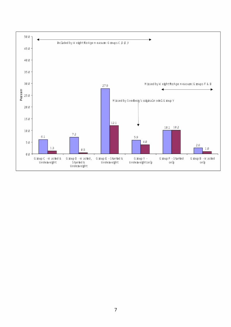
Rates of stunting, wasting and underweight (at both mild/moderate and severe levels) in children of this age were calculated using height and weight data. A CIAF for the same children was then constructed. During the process, an additional group of anthropometric failure - Group Y - emerged, which did not appear in Svedberg's original model. The model was therefore modified to show this group (Figure I.2). Group Y includes those children who are underweight but who are not wasted or stunted.

Figure I.2: Anthropometric failure combinations (groups A to F and new group Y)

Group Y may have been overlooked because the original model assumed the diagonal Weight for Height line passes through the origin of the Weight for Age and Height for Age axes (see Figure I.1). However, the axes in Figure I.1 represent deviations from the Height for Age and Weight for Age axes. Figure I.2 shows the modification made to Svedberg's original model, with the Weight for Height line passing through the correct origin of the Height for Age and Weight for Age axes.

The CIAF therefore covers all children who are wasted and/or stunted and/or underweight, while other measures appear to miss different sets of children. Figure I.3 illustrates how children are 'missed', using the Weight for Age indicator (Underweight) as an example. The CIAF shows that at the mild/moderate level (i.e. <-2SD), 59.8% of children are in fact malnourished – considerably more

4

than suggested by the conventional indicies. At the ‘severe’ level (i.e. <-3SD), the CIAF shows 29.1% of children in India 0-35 months are severely malnourished.

Figure I.3: Malnourished children missed by the underweight measure

5

6

SECTION II

STANDARD OF LIVING INDICES

IntroductionStrong associations have been found between low socio-economic position (SEP) and poor health (WHO, 1995). The construction of socio-economic indices is one of the most economically important uses of social statistics, since they often contribute as key elements in the allocation of resources. Here, data collected by the National Family Health Survey (NFHS) 1998-1999 (IIPS, 2000f) was used to calculate two standard of living indices. Such indices are used to determine whether there is an association between socio-economic deprivation and health.

Weighting of indicesOut of necessity, many standard of living indices are often composed of indirect or proxy indicators rather than direct measures. It is, therefore, unsurprising that a bewildering array of indices has been proposed, using different combinations of variables and different statistical methods.

The key question that most researchers want answered is ‘which index is the best?’ This question can be divided into two parts: firstly, what does the index measure (if anything) and, secondly, ‘which index provides the most accurate and precise measurement?’ Answering these questions is often far from a simple matter. Advocates of new indices rarely make detailed comparisons between their index and others. Similarly, theoretical discussions on the nature and measurement of socio-economic conditions and health are often dealt with in a cursory manner or are entirely lacking from many papers. Indeed, many indices seem to be composed from combinations of variables that the authors think measure something ‘bad’ or ‘harmful’. Although, what these ‘bad’ things are is often unclear. Various statistical procedures and transformations are often performed on the indices components, usually in order to ensure equal weighting, i.e. so that each variable provides an equal contribution to the final index. However, the justification for such statistical procedures is often absent. The terms ‘health’, ‘standard of living’ and ‘poverty’ are generally used loosely, with little reference to the specific technical meanings of these terms (Gordon, 1995).

The need for weightingSocial scientists have been using social surveys to study poverty and health in Britain for over a hundred years. All these surveys have shown that certain groups are more likely to suffer from multiple deprivation and ill health than others (i.e. disabled people and the unemployed are not equally likely to be living in poverty or suffering from ill health and indices that consider them to be are probably wrong.) Similar results have been found from India and other countries. Therefore, deprivation and health indices that give equal weight to their component variables are likely to yield inaccurate results.

7

For example, in India in the early 1990s, the ‘fulfilment of basic needs’ survey in West Bengal (Rudra et al, 1994; Joshi, 1997) measured the standard of living of poor households using the following 17 indicators:

1. Consumption of meat, fish and egg during last month.2. Number of bedrooms (<1) per family.3. Room height (<1.68 meters).4. Adequacy of dwelling for protection against room shows.5. Woollen garments in the household.6. Number of woollen garments (<1) per person.7. Number of saris or similar garments (<2) per adult female.8. Mattresses in the bedding.9. Lack of blankets, quilts in the households.10. Number of dining plates (<1) per adult member.11. School education for child of age group 6-14.12. Availability of two square meals a day through out the last year and, if not, whether the

number of months when they did not get this was >2.13. Availability of milk every day for children in the age group (0-4).14. Member of household engaged in begging.15. Availability of special food before and after delivery for female member who conceived

during last three years.16. Whether or not the household procured food items as gift or loan from some other

household during last month.17. Whether or not the household usually obtained food items by free collection from months

or from land belonging to other.

The authors of this study, quite correctly, determined that these 17 poverty indicators were not all of equal importance. Households were assigned, by deprivation score and simple pragmatic criteria, to three levels of poverty (first, second and third level of poverty).

The first level of poverty was defined as ‘ultra poor’ on the basis of at least one of the following three criteria.

Non-availability of two square meals a day for more than two months during the last year. Non-availability of saris or similar garments per adult female in the house being less than

two. Member of household reporting begging.

The second level of poverty included households with a deprivation score of 4 or more and the number of months without two square meals a day was two or more.

The third level of poverty was defined by deprivation score of 1 to 3 and the number of months without two square meals a day was either none or one.

Since most social survey based indices are generally composed of indicators of unequal importance or even of surrogate or proxy measures of deprivation and health rather than direct measures, there are two basic requirements they should fulfil to ensure accuracy:

The components of the index should be weighted to reflect the different probability that each group has of suffering from deprivation and/or ill health; and

8

the components of the index must be additive, e.g. if an index is composed of two variables, unemployment and lone parenthood, then researchers must be confident that unemployed lone parents are likely to be poorer or less healthy than either lone parents in employment or unemployed people who are not lone parents.

Weighted indices also have the advantage that their results are often much easier to understand, e.g. saying that, in a given area, 25% of households are living in poverty has a much greater intuitive meaning than saying that an area has a Z-score of 7.86 or a signed Chi-squared score of 22.46.

Methods of weighting indicesWhere researchers are very experienced, it is often possible for them to produce very good pragmatic weightings based on a lifetime of research experience. However, few people have this level of in-depth knowledge and most have to rely on more formal methods. There are some general and proven methods of weighting indices that have been developed by European researchers (particularly Dutch, Swedish, Irish, Portuguese and British social scientists).

Possession weighting Proportionate possession weighting Opinion weighting Proportionate opinion weighting

Possession weighting was suggested by Peter Townsend (1979) in his study of Poverty in the United Kingdom. It involves measuring the normal level of possession for standard of living or health measures and then weighting each component of an index by this level (or its inverse). For example, if 90% of all households can manage to obtain a school education for their children aged 6-14 and 98% of all households do not need to engage in begging, then these two components of a deprivation index could be given a weighting of 90 and 98, respectively. Those households with the highest score on this index would be the most deprived (poorest). Alternatively, if the purpose is to construct a standard of living index rather than a deprivation index, then the same two items could be given a weighting of 10 (100-90=10) and 2 (100-98=2), respectively. Those households with the highest score on this index would be the wealthiest (richest). The possession weighting method has been widely used by European social scientists, particularly when comparing survey results from different countries or from different years in the same country (for example, see Nolan and Whelan, 1996; Gordon and Pantazis, 1997; Gordon et al, 2000; Layte et al, 2001).

Proportionate possession weighting (PPW) is an adjustment that reflects the differences between various social and demographic groups. Thus, the PPW approach takes account of these differences by adjusting the weighting for each index item according to significant differences within the population. Account could be taken of the variation in the preferences of any number of different social or demographic groups, such as - sex, age, family composition (whether they are single or couples with or without children) or rurality. Proportionate index weights would allow for differences in, for example, the different levels of possession of electricity and bullock carts between urban and rural households.

Opinion weighting has been used widely in both poverty and health research. For example, Joanna Mack and Stewart Lansley conducted social surveys in the UK to determine the population’s views on what were the ‘necessities of life’. They then produced deprivation indices that were weighted by public opinion and thus went further than any of their predecessors in an effort to relate the definition of poverty to the view of public opinion and to reduce the impact of arbitrary decisions.

9

“.....we have aimed to exclude our own personal value judgements by taking the consensual judgement of society at large about people’s needs. We hope to have moved towards what Sen describes as ‘an objective diagnosis of condition’ based on ‘an objective understanding of ‘feelings’.” (Mack and Lansley, 1985, p46)

Similarly, a number of different measures of health have made use of public opinion on the desirability (or lack of it) of various health conditions to produce opinion weighted health indices (e.g. EuoQol 5D, Qualy’s, etc.).

Proportionate opinion indices have not yet been used to any great extent in health research but have been used more widely in the study of poverty and deprivation. Such indices have been used extensively in Scandinavian research where public opinion on the minimum acceptable standard of living has been used to produce indices that are weighted to reflect those differences by sex, age and family composition (whether they are single or couples with or without children). This method of weighting to measure poverty has been called the ‘proportional deprivation index’ (PDI). It has been argued that the PDI is more theoretically appealing than more simple deprivation indices since it is more sensitive to individual preferences and takes account of significant differences in preferences between demographic and social categories (Halleröd, 1994; 1995; 1998; Halleröd, Bradshaw and Holmes, 1997).

Weighting and statistical theoryWeighting is an important part of valid and reliable index construction, particularly where only a limited number of proxy indicators are available. However, if large numbers of direct measures are available to the researcher, then weighting is of lesser concern since both statistical theory and empirical research has shown that indices with equal weights for each component can perform almost as well as weighted indices given sufficient high quality measures of health and standard of living.

The NFHS Standard of Living IndexA standard of living index was created by the NFHS as a summary household measure (IIPS, 2000). It is composed of 27 items, including consumer durables, agricultural machinery, housing conditions and access to basic services (water, light, fuel, etc). The components of the NFHS index are set out in Table II.1, together with their respective weights.

Table II.1: NFHS Standard of Living Index components and weights

Household characteristic Scores1 House type - pucca =4 - semi pucca=2 - kachha=02 Separate room for cooking - yes=1 - no=03 Ownership of house - yes=1 - no=0

10

4 Toilet facility - own flush toilet=4

- public or shared flush toilet or own pit toilet=2

- shared or public pit toilet=1

- no facility=0

5 Source of lighting - electricity=2 - kerosene, gas, oil=1

- other source of lighting=0

6 Main fuel for cooking- electricity, liquid petroleum gas or biogas=2

- coal, charcoal or kerosene=1 - other fuel=0

7 Source of drinking water

- pipe, hand pump, well in residence/ yard/ plot=2

- public tap, hand pump or well=1

- other water source=0

8 Car or tractor - yes=4 - no=09 Moped or scooter - yes=3 - no=010 Telephone - yes=3 - no=011 Refrigerator - yes=3 - no=012 Colour TV - yes=3 - no=013 Black and white TV - yes=2 - no=014 Bicycle - yes=2 - no=015 Electric fan - yes=2 - no=016 Radio - yes=2 - no=017 Sewing machine - yes=2 - no=018 Mattress - yes=1 - no=019 Pressure cooker - yes=1 - no=020 Chair - yes=1 - no=021 Cot or bed - yes=1 - no=022 Table - yes=1 - no=023 Clock or watch - yes=1 - no=024 Ownership of livestock - yes=2 - no=025 Water pump - yes=2 - no=026 Bullock cart - yes=2 - no=027 Thresher - yes=2 - no=0

The index is calculated by summing the weights which have been developed by the International Institute of Population Sciences NFHS research team in India. These weights are based upon their considerable knowledge of the relative significance of ownership of these items, rather than on a more formal analysis. For example, a household which owns a colour TV is considered to be three times as wealthy as one that owns its own house (IIPS, 2000).

The NFHS Standard of Living Index was created for All India as well as for each state (Andhra Pradesh, Madhya Pradesh, Orissa, West Bengal) with possible scores ranging from 0-67.

For the purpose of comparison, the index was grouped into quintiles based on a reference population consisting of the 1999 All India NFHS-2 data set. The first quintile represents the poorest group of the population and the fifth represents the wealthiest.

Standard of Living Index (SLI) using a Proportionate Possession Weighting (PPW)Very experienced researchers like the IIPS team can develop weightings for standard of living items based upon their experience. However, a more generalised method of weighting is also desirable,

11

which can produce consistent results for different surveys across both time and place. Many researchers simply select a group of standard of living items and sum them (e.g. all items have a weight of one). This is obviously not the best method when comparing different areas since the possession of different standard of living indicators may signify different degrees of wealth from one place to another, e.g. the ownership of a colour television in India (where few households have one) is highly likely to indicate a greater degree of relative wealth than the ownership of a colour television does in the UK, where most households possess one. Conversely, owning your own home in the UK (where land prices are relatively high) is likely to be a better indicator of wealth than home ownership is in India, where land prices are relatively low.

An alternative standard of living index was calculated using a different method of weighting the indices. A proportionate possession weighting (PPW) is an adjustment that reflects the differences between various social and demographic groups and , therefore, takes account of these differences within the population. Unlike the NFHS Standard of Living Index, this PPW index refers entirely to a household’s possessions. For example, proportionate index weight would allow for differences in the various levels of possession of telephones and tables between urban and rural households.

Elements such as ‘water source’ or ‘toilet facility’ can often be considered public goods and can be more representative of a village’s standard of living than that of an individual household within the village. Rather than using a system of independently attributed scores, this SLI uses the relative proportion of each possession as scores reflecting the significant differences specific to the population in question. For example, 1.6% of households in the All India sample own a car. Using the PPW method, car owners would be assigned a score of 98.4 (100-1.6). The proportions of each possession were taken from the NFHS-2 All India report (IIPS, 2000).

The possessions included in the PPW are set out in Table II.2, together with their All India weightings.

The PPW indicesThree separate indices were created using the All India possession proportions:

Overall All India SLI: applying the all India possession weightings to the data. Rural All India SLI: applying the all India rural possession weightings to the data. Urban All India SLI: applying the all India urban possession weightings to the data.

Furthermore, a PPW index was created based on the possession proportions of each of the four states:

Andhra Pradesh state SLI: applying the Andhra Pradesh specific possession weightings to the data.

Madhya Pradesh state SLI: applying the Madhya Pradesh specific possession weightings to the data.

Orissa state SLI: applying the Orissa specific possession weightings to the data West Bengal state SLI: applying the West Bengal specific possession weightings to the

data.

See Tables A.1 to A.4 in the Appendix for the weights for the four states.

12

Table II.2: Proportionate Possessions Weighting based on NFHS All India 1998 Report

All India total All India urban All India ruralItem % weight % weight % weight

1 Mattress 47.4 52.6 71.7 28.3 38.1 61.92 Pressure cooker 29.6 70.4 65.2 34.8 16.0 84.03 Chair 45.5 54.5 71.3 28.7 35.6 64.44 Cot/bed 81.2 18.8 86.1 13.9 79.4 20.65 Table 39.6 60.4 64.9 35.1 30.0 70.06 Clock/watch 66.5 33.5 90.1 9.9 57.5 42.57 Electric fan 45.5 54.5 82.2 17.8 31.4 68.68 Bicycle 47.8 52.2 53.5 46.5 45.7 54.39 Radio 38.0 62.0 53.2 46.8 32.2 67.810 Sewing machine 18.4 81.6 35.5 64.5 11.9 88.111 Telephone 7.4 92.6 20.1 79.9 2.6 97.412 Refrigerator 10.6 89.4 28.8 71.2 3.7 96.313 TV (B/W) 24.7 75.3 44.8 55.2 17.0 83.014 TV (colour) 10.1 89.9 27.3 72.7 3.5 96.515 Moped 11.2 88.8 25.0 75.0 6.0 94.016 Car 1.6 98.4 4.4 95.6 0.6 99.417 Tractor 1.6 98.4 0.8 99.2 2.0 98.018 Bullock cart 7.2 92.8 1.4 98.6 9.4 90.619 Water pump 8.5 91.5 9.3 90.7 8.2 91.820 Thresher 2.0 98.0 0.7 99.3 2.5 97.5

The relative differences between the NFHS index and PPW index weighting schemes are shown in Figures II.4 and II.5 below.

13

Figure II.4: NFHS weights for each possession

Figure II.5: PPW weights for each possession

14

Figures II.4 and II.5 show that the two weighting schemes broadly correspond, with the PPW index giving a relatively greater weight than the NFHS index to pressure cooker, table, sewing machine, water pump, bullock cart and thresher.

The Theory of MeasurementIt is of crucial importance to this research to establish that the NFHS and PPW indices are ‘good’ measures of standard of living. In order to establish this it is necessary to understand measurement theory. Classical test theory dates back to the pioneering work of Spearman (1904) and others at the turn of the century and much of the modern theoretical work has been developed by educationalist and psychologists since the Second World War. Classical test theory distinguishes between the observed score (measurement) on any test and the ‘true’ score. Since all attempts to measure anything will inevitably result in some random errors creeping in to the measurement, the observed score is comprised of two components - the true score and random error:

O = T + RE

where:O = Observed scoreT = True scoreRE = Random error

The true score (in this case the true level of standard of living) is of course a hypothetical quantity. It can never be measured directly, only estimated from the observed score and a knowledge of the size of the random measurement errors. If the size of the random errors is large relative to the observed score, then the measurement is unreliable by definition. Conversely, if the random errors are small, the measurement is reliable. The concept of reliability in this sense is equivalent to the concept of precision used in the natural sciences.

There are a large number of sources of random error that have been catalogued in the literature in relation to social surveys, such as Censuses and deprivation studies. These range through mis-codings, ambiguous instructions, different emphasis on different words during an interview, interview fatigue, etc. This means that “the amount of chance error may be large or small, but it is universally present to some extent. Two sets of measurements of the same features of the same individual will never exactly duplicate each other” (Stanley, 1971)

Thus, all measurements are, to some extent, unreliable. What is important is the degree of unreliability.

However, random errors are not the only type of errors present during measurement (of deprivation or anything else). In addition, there are always systematic errors or biases present. There are many sources of bias recorded in the literature which include, for example, people giving incorrect information because they are embarrassed by their standard of living or income, response-set (where a person repeatedly answers ‘yes’ or ‘no’ to a series of questions because they have lost concentration), or the tendency for the elderly to over-estimate their level of good health, etc.

Thus, Spector (1994) has argued that classical test theory can be extended so that the observed scores can be considered to be comprised of the true scores plus random and systematic errors:

O = T + RE + SE

15

where:O = Observed scoreT = True scoreRE = Random errorSE = Systematic error

A valid measurement is one where the size of the systematic error is small. The concept of validity is analogous to the concept of accuracy used in the natural sciences. However, this mathematical formulation of validity to some extent begs the question. A measurement cannot be generally valid - it must be valid for something, for example, a driving test may be a valid test of the driver’s ability to control the car but it is probably not a valid test of the driver’s ability to tap dance or get a degree in mathematics. Validity can only be assessed in relation to a theoretical framework.

ReliabilityThe term ‘reliability’ often causes confusion because the common usage of the word differs from its scientific meaning. In common usage, a reliable measurement is a correct measurement, eg something that can be relied upon. However, in scientific terms, a reliable measurement is not necessarily correct - it is just precise. For example, if you were to repeatedly measure an object with a one foot ruler, which in reality was only 11 inches long, you would produce a series of very similar measurements. This series of measurements would be highly reliable even though they were completely inaccurate. Scientific reliability is about the consistency of a measurement, not its accuracy and there are a number of statistics that can be used to measure the internal consistency (reliability) of scales such as standard of living indices.

Reliability of the NFHS and PPW indices All measurement is subject to error which can take the form of either random variations or systematic bias (Stanley (1971) lists many causes of bias). Random errors of measurement can never be completely eliminated. However, if the error is only small relative to size of the phenomena being studied, then the measurement will be reliable. Reliable measurements are repeatable, they have a high degree of precision.

The theory of measurement error has been developed, mainly by psychologists and educationalists, and its origins can be traced to the work of Spearman (1904). The most widely used model is the Domain-Sampling Model, although many of the key equations can be derived from other models based on different assumptions (see Nunnally (1981) Chapters 5-9, for detailed discussion).

The Domain-Sampling Model assumes that there is an infinite number of questions (or, at least, a large number of questions) that could be asked about deprivation. If you had an infinite amount of time, patience and research grant, you could ask every person/household all of these questions and then you would know everything about their level of deprivation, i.e. you would know their ‘true’ deprivation score. The 20 questions used in the PPW standard of living index can be considered to be a subset of this larger group (domain) of all possible questions about standard of living.

Some questions will obviously be better at measuring standard of living than others, however, all of the questions that measure standard of living will have some common core. If they do not, they are not measuring deprivation - by definition. Therefore, all the questions that measure deprivation should be intercorrelated so that the sum (or average) of all the correlations of one question, with all

16

the others, will be the same for all questions (Nunnally, 1981). If this assumption is correct then, by measuring the average intercorrelation between the answers to the set of deprivation questions, it is possible to calculate both:

an estimate of the correlation between the set of questions and the ‘true’ scores that would be obtained if the infinite set of all possible standard of living questions had been asked; and

the average correlation between the set of questions asked (the standard of living index) and all other possible sets of deprivation questions (standard of living indices) of equal length (equal number of questions).

Both these correlations can be derived from Cronbach’s Coefficient Alpha (Cronbach, 1951; 1976; Cronbach et al, 1971).

Cronbach’s Coefficient Alpha is 0.86 for the 20 items used in the PPW SLI. This is the average correlation between these 20 items and all the other possible sets of 20 items that could be used to measure standard of living. The estimated correlation between the 20 items and the ‘true’ scores, from the infinite possible number of standard of living questions, is the square root of Coefficient Alpha, i.e. 0.93.

Nunnally (1981) has argued that:

“in the early stages of research ... one saves time and energy by working with instruments that have modest reliability, for which purpose reliabilities of 0.70 or higher will suffice ... for basic research, it can be argued that increasing reliabilities much beyond 0.80 is often wasteful of time and funds, at that level correlations are attenuated very little by measurement error.”

Therefore, the Alpha Coefficient score of 0.86 for the 20 PPW index items indicates that they have a high degree of reliability and also that effectively similar results would have been obtained if any other reliable set of 20 standard of living questions had been asked instead.

Table II.3: Reliability analysis of components of PPW SLI score

Components of PPW SLI score Corrected item total correlation

Alpha Coefficient if item deleted

Mattress 0.597 0.797Pressure cooker 0.610 0.797Chair 0.606 0.797Cot or bed 0.331 0.812Table 0.629 0.796Clock or watch 0.557 0.800Fan 0.613 0.796Bicycle 0.339 0.813Sewing machine 0.479 0.806Telephone 0.423 0.810Refrigerator 0.488 0.807Television (B/W) 0.375 0.810Television (colour) 0.431 0.809Car 0.228 0.817

17

Water pump 0.317 0.813Bullock cart 0.119 0.819Thresher 0.146 0.818Tractor 0.191 0.817Radio 0.455 0.806Moped 0.485 0.807Ownership of house -0.002 0.824Ownership of land 0.026 0.831Ownership of livestock -0.045 0.835

N of Cases 92235N of Items 23

Alpha Coefficient 0.818

Coefficient alpha can also be used to test the reliability of individual questions. Table II.3 shows how the Alpha Coefficient would change if any single question was deleted from the deprivation index. There are only three questions (highlighted in bold) which would yield an increase in Alpha Coefficient when removed, i.e. ownership of house, land or livestock.

However, it is important to examine the reasons why these three items are not reliable measurers of standard of living. Ownership of a house and livestock are negatively correlated with the standard of living scale, which may indicate that, in India, many owner-occupier households with some animals tend to have a lower standard of living than other households. Similarly, the ownership of a small amount of land may not indicate a high standard of living, e.g. small farmers are often ‘poorer’ than urban households.

Therefore, based on this initial reliability analysis, where the Alpha Coefficient was already high (0.82), the items highlighted in bold, ownership of house, land and livestock were removed from the score in order to improve the internal consistency of the index. Based on these corrections the Alpha Coefficient of the PPW SLI score improved to 0.86.

The same analysis carried out on the 27 components of the NFHS SLI (see Appendix for components) gave the following inter-item correlation – Alpha Coefficient – 0.79.

Based on these Alpha coefficients, both scales are reliable. The 20 item PPW index is a more reliable scale, with 74% of the variance explained by the internal components. The 27 item NFHS index is also reliable, with 62% of the variance explained by the internal components. Though the PPW scale is more reliable, these analyses do not provide information on the validity of the respective index.

Validity of the NFHS and PPW Standard of Living Indices In order to be a ‘good’ measure of standard of living, an index must be both reliable and valid (precise and accurate in the terminology of the natural sciences). There are several types of validity measures.

Face Validity The standard of living measures in both the NFHS and PPW indices have a high degree of face validity. Anastasi (1988) describes the concept of face validity as follows:

18

"Content validity should not be confused with face validity. The latter is not validity in the technical sense; it refers, not to what the test actually measures, but to what it appears superficially to measure. Face validity pertains to whether the test "looks valid" to the examinees who take it. the administrative personnel who decide on its use, and other technically untrained observers (p.144)."

Therefore, face validity is concerned with how a measure or procedure appears. Unlike content validity, face validity does not depend on established theories for support (Fink, 1995). Possession of consumer durables and housing facilities has been shown in all countries to be associated with standard of living e.g. the higher the standard of living of a household the more possessions they tend to have and the better their housing conditions. In general, the ‘rich’ do not choose to live like the ‘poor’ in any country and the ‘poor’ generally lack possessions due to a lack of resources rather than out of choice. It is also fairly evident that the possessions used in the two indices are relevant measures of standard of living in the Indian context (they have face validity) compared with the type of items that are often used in, say, Nordic countries, e.g. cross country skis, small boats, mobile phones, etc.

Construct ValidityThere are many types of validation procedures, however the most commonly applicable to the social sciences is construct validation. Construct validation is based on assessing how well a “particular measure relates to other measures consistent with theoretically derived hypotheses concerning the concepts (or constructs) that are being measured.” (Carmines and Zeller, 1994).

In the case of standard of living theory it is predicted that those who are ‘poorest’ are more likely to suffer from ill health than those with a higher standard of living. Therefore, it would be expected that areas with high levels of poverty would also be areas with high levels of ill health (all other things being equal). Similarly, theory predicts that people suffering from a low standard of living are also likely to suffer from a range of deprivations, for example, food deprivation (e.g. food of insufficient quantity and/or quality). Therefore, an area with low levels of standard of living is also likely to contain food deprived households. Therefore indicators of ill health and severe deprivation can be used as validation criteria for assessing the construct validity of standard of living indices, eg the most valid (accurate) indices are likely to be those with the highest correlations with ill health and severe deprivation.

A frequently asked question is ‘why bother to go to all the trouble of constructing both a standard of living index and a measure of ill health and then working out the correlation between them? Why not simply use the measure of ill health as a proxy index for standard of living?’ The direction of causality is the key to the answer; the relative theory of poverty predicts that poor people are likely to become sick, not that sick people are likely to become poor (Lee et al, 1995). Indeed, theories that predict that sick people are likely to become poor have been shown to be of only limited validity in the European context (Power et al, 1990). This is not to deny that ill health can cause a fall in the standard of living of a household, this is an undeniable fact in all countries. However, although this reciprocal causality exists (poverty causes ill health and ill health can cause poverty), longitudinal studies have shown that far more ill health is caused by poverty, than poverty is caused by ill health.

It is well established that a low standard of living is strongly associated with poor outcomes for both adults and children. In particular, in developing countries, household deprivation and a lack of control of sufficient resources over time often results in anthropometric failure in younger children, particularly stunting (low height for age). A good measure of the validity of each component of the

19

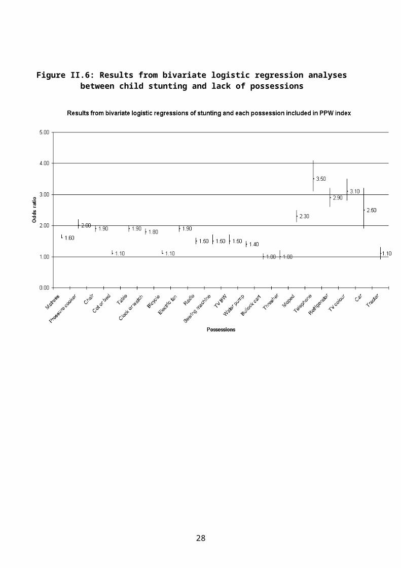
NFHS and PPW standard of living indices is to calculate the likelihood that the children (under two years) in a household will suffer from stunting if they lack an item in the index.

Figure II.6 and Table II.4 below show the results of a criterion validity exercise at the individual level, they display the results from a series of bivariate logistic regression analyses for the odds of stunting in children if a household lacks a standard of living item.

Figure II.6: Results from bivariate logistic regression analyses between child stunting and lack of possessions

20

Table II.4: Comparison of the odds ratio for stunting to the index weights for each possession

21

Figure II.6 and Table II.4 show that a household that does not have a telephone or a colour TV is 3.5 times more likely to have a stunted child than a household that owns a telephone. Households which own a colour television are three times less likely to have stunted children than households that do not. Similarly, children in households that possess refrigerators or mopeds or pressure cookers are half as likely to suffer from stunting than households which do not own these items. These consumer durables seems to be valid measures of standard of living. Conversely, children in households which own tractors, threshers and bullock carts are not significantly more likely to be stunted than those in households which do not. These agricultural possessions are likely to be somewhat invalid measures of standard of living. In the case of tractors and threshers, the lack of validity on this test is mainly due to the relatively small number of households in the survey which own these items and also have children aged under two.

It would be possible to create a somewhat more reliable and valid index for India by dropping the agricultural items from the PPW SLI, however, it was decided not to do this in order to maintain comparability between the NFHS standard of living index and the PPW index. Also, dropping all the agricultural items from the PPW standard of living index would reduce its reliability, without much gain to the index’s validity.

For this research, the main purpose of measuring standard of living was to obtain a reliable ranking of households from ‘richest’ to ‘poorest’ within and between states. It was therefore more important to maximise the reliability of the index than to maximise its validity. The PPW standard of living index was therefore designed to demonstrate that standard scientific index construction methods could allow researchers who do not possess a lifetime of knowledge on standard of living in India to produce a highly reliable (and also valid) index while also maintaining a high degree of comparability with previous research in this field.

It must be noted that different approaches can be used to construct standard of living indices, other than classical test theory. In particular, several researchers have used a factor analyses framework to build valid and reliable indices of standard of living. The most comprehensive comparative research in this area has recently been undertaken by the New Zealand Government (Krishnan, Jensen and Ballantyne, 2002). Which compared the results of standard of living indices constructed on the basis of an extensive confirmatory factor analysis approach with one constructed using a classical test theory approach (Item Response Theory) (see Reise, Widaman and Pugh, 1993; Jensen et al, 2002). They found that both approaches produced standard of living indices with similar properties but for policy purposes the classical test theory approach index was the most suitable. Detailed confirmatory factor analysis models are often both very complex and time consuming and subject to the danger of ‘overfitting’ the model. This can result in an index which is specific to a certain dataset rather than being more generalisable. Simpler factor analysis approaches, like principal components analysis, can result an index whose meaning is difficult to interpret (for an Indian example see Filmer and Prichett, 2001)

Comparing the indices

All India overall indicesThe indices were first compared at the All India scale through the use of Pearson’s correlation coefficients. When the overall All India NFHS and PPW indices were compared, Pearson’s correlation gave a figure of 0.96 (correlation is significant to the 0.01 level (two tailed).

The positive correlation between the two indices is very high and can be highlighted graphically by a scatter-plot comparing the household SLI scores from each index.

22

Figure II.7: Scatter plot of All India overall NFHS and PPW standard of living indices

The Pearson’s coefficient and the scatter plot confirm that the two indices are highly correlated, with 92% of the variance being explained by this association.

All India urban indicesThe urban indices were compared at the All India scale through the use of Pearson’s correlation coefficients, using data for urban households only. The NFHS index was compared to the PPW index that uses All India urban possession weightings (see Appendix). Pearson’s correlation gave a figure of 0.95 (correlation is significant to the 0.01 level (two tailed).

The positive correlation between the two indices is very high and can be highlighted graphically by a scatter-plot comparing the household SLI scores from each index:

23

Figure II.9: Scatter plot of All India urban NFHS and PPW standard of living indices

The Pearson’s coefficient and the scatter plot confirm that the two urban indices are highly correlated, with 90% of the variance being explained by this association.

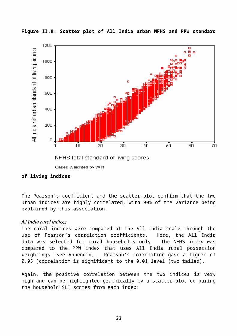
All India rural indicesThe rural indices were compared at the All India scale through the use of Pearson’s correlation coefficients. Here, the All India data was selected for rural households only. The NFHS index was compared to the PPW index that uses All India rural possession weightings (see Appendix). Pearson’s correlation gave a figure of 0.95 (correlation is significant to the 0.01 level (two tailed).

Again, the positive correlation between the two indices is very high and can be highlighted graphically by a scatter-plot comparing the household SLI scores from each index:

24

Figure II.8: Scatter plot of All India rural NFHS and PPW standard of living indices

The Pearson’s coefficient and the scatter plot confirm that the two rural indices are also highly correlated, with 90% of the variance being explained by this association.

Comparing the indices within the four states

Understanding the indicesIn all four states two sets of proportionate possession weighted indices were produced,

1) an All India set of weighted indices to facilitate comparisons between urban and rural areas in each state and the urban and rural Indian average distribution and,

2) a set of state weighted indices to facilitate the comparison of the relative distribution of wealth between urban and rural areas within the state.

The details of each index are described below;

NFHS overall index: This is the NFHS SLI applied to the state in question.

25

All India PPW index: The NFHS-2 All India data set was used to extract proportions of materials/goods owned. These proportions form the basis for constructing an All India PPW index applied to the state in question.

State PPW index: The particular NFHS-2 state data set was used to extract proportions of materials/goods owned. These proportions form the basis for constructing a state PPW index.

NFHS urban index: This is the NFHS SLI applied to urban areas of the state in question.

All India urban PPW index: The NFHS-2 All India urban data set was used to extract proportions of owned materials/goods. These proportions form the basis for constructing an All India PPW index applied to urban areas of the state in question.

NFHS rural index: This is the NFHS SLI applied to rural areas of the state in question.

All India rural PPW index: The NFHS-2 All India rural data set was used to extract proportions of materials/goods owned. These proportions form the basis for constructing an All India PPW index applied to rural areas of the state in question.

Andhra PradeshThree forms of standard of living indices were calculated for Andhra Pradesh: three All India weighted PPW indices (overall, rural, urban), a state weighted PPW index and an NFHS index (see Appendix for weightings).

Comparing Andhra Pradesh and All India indices using correlationsThe Andhra Pradesh NFHS and All India weighted PPW indices were compared using Pearson’s correlation coefficients. This gave a correlation of 0.96 (correlation is significant to the 0.01 level (two tailed).


26

Figure II.9: Scatter plot of Andhra Pradesh NFHS and All India weighted PPW SLI

The Pearson’s coefficient and the scatter plot confirm that the two indices are highly correlated, with 92% of the variance being explained by this association.

Comparison between Andhra Pradesh indices using quintile distributionAll of the standard of living indices were divided by referent quintiles using NFHS-2 All India data to establish the quintile cut-offs. Below, the NFHS index is compared to the PPW index by presenting the data in quintile form. The percentage of households in each SLI referent quintile is shown providing a comparison between the two indices and also with the All India average. The lowest quintile represents the most deprived households.

27

Figure II.10: All India overall indices calculated for Andhra Pradesh: % of households by NFHS and PPW SLI shown in quintiles

The above chart illustrates the distribution of standard of living within the state of Andhra Pradesh using two independent methods of calculation. The differences between the NFHS and PPW methods of calculating standard of living are relatively small. Both indices show a similar trend: a larger proportion of the Andhra Pradesh population is present in the lowest standard of living quintile. Using both indices, the lowest proportion of households is present in the highest quintile. Compared to the All India sample, Andhra Pradesh has a larger proportion in the most deprived quintile and a lower than average proportion in the wealthiest quintile. This was a consistent finding using both indices.

28

Figure II.11: All India urban indices calculated for Andhra Pradesh: % of urban households by NFHS and PPW SLI shown in quintiles

The above chart illustrates the distribution of standard of living within the urban households of Andhra Pradesh using two independent methods of calculation. The differences between the NFHS and PPW methods of calculating standard of living are relatively small, with similar variations occurring across the quintile range. Both indices show a gradient with the largest proportions of Andhra Pradesh households in the lowest quintiles and the lowest proportions in the highest quintiles. Furthermore, compared to the All India sample, Andhra Pradesh has a larger proportion of its urban households in the most deprived quintiles and fewest households in the wealthy quintiles.

29

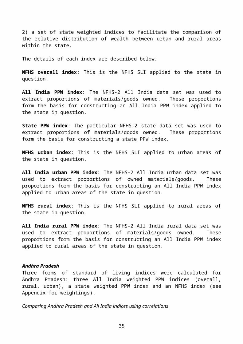
Figure II.12: All India rural indices calculated for Andhra Pradesh: % of rural households by NFHS and PPW SLI shown in quintiles

The above chart illustrates the distribution of standard of living within the rural households of Andhra Pradesh using two independent methods of calculation. The differences between the NFHS and PPW methods of calculating standard of living are relatively small, with similar variations occurring across the quintile range. Both indices show that the largest proportion of the rural population is present in the lowest standard of living quintile. With both indices, the lowest proportion of households is present in the second quintile. Furthermore, compared to the All India rural sample, Andhra Pradesh has a larger proportion of its rural households in the most deprived quintile.

The above indices, calculated from All India data and using the NFHS methods, show that most of the households in Andhra Pradesh are found in the poorest SLI quintiles compared to the All India average. This was true for both rural and urban households in Andhra Pradesh when they were observed independently.

30

Comparing Andhra Pradesh indices using correlationsThe Andhra Pradesh NFHS and state weighted PPW indices were compared using Pearson’s correlation coefficients. The correlation found was 0.96 (correlation is significant to the 0.01 level (two tailed).


Figure II.13: Scatter plot of Andhra Pradesh NFHS and state PPW SLI

The Pearson’s coefficient and the scatter plot confirm that the state PPW and NFHS indices are highly correlated, with 92% of the variance being explained by this association.

Comparison within Andhra Pradesh state PPW indexThe Andhra Pradesh state weighted SLI provides a comprehensive reflection of the socio-economic differentials within the state. Below, it is divided by Andhra Pradesh overall referent quintiles, allowing for a comparison between rural and urban households and the Andhra Pradesh average SLI distribution.

31

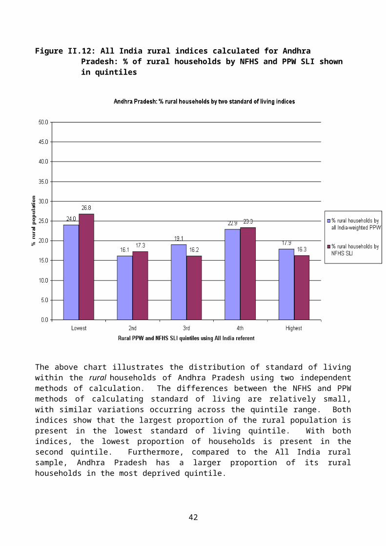
Figure II.14: State PPW index calculated for Andhra Pradesh: % of urban and rural households by state PPW SLI shown in quintiles

The above chart illustrates the distribution of standard of living within the rural and urban households of Andhra Pradesh using a state weighted index. The differences between urban and rural households within Andhra Pradesh and compared to the state average are striking. Urban households are present in a steep gradient across the quintile range, with the lowest proportion (6%) in the poorest quintile and the highest proportion (45%) in the wealthiest quintile. By contrast, rural households show an opposite trend. The largest proportion of rural households are in the most deprived quintiles and the lowest proportion is in the wealthiest quintile. Compared to the Andhra Pradesh average, an extra 25% of urban households and 8% fewer rural households are present in the highest quintile. Using the state weighted PPW index allows insights into the relative distribution of wealth within the state.

Madhya PradeshThree forms of standard of living indices were calculated for Madhya Pradesh: three All India weighted PPW indices (overall, rural, urban), a state weighted PPW index and an NFHS index (see Appendix for weightings).

Comparing Madhya Pradesh and All India indices using correlationsThe Madhya Pradesh NFHS and All India weighted PPW indices were compared using Pearson’s correlation coefficients. This gave a correlation of 0.97 (significant to the 0.01 level (two tailed).

32


Figure II.15: Scatter plot of Madhya Pradesh NFHS and All India weighted PPW SLI

The Pearson’s coefficient and the scatter plot confirm that the All India PPW and NFHS indices are highly correlated, with 92% of the variance being explained by this association.

Comparison between Madhya Pradesh standard of living indices All of the standard of living indices were divided by referent quintiles using NFHS-2 All India data to establish the quintile cut-offs. Below, the NFHS index is compared to the PPW index by presenting the data in quintile form. The percentage of households in each SLI referent quintile is shown providing a comparison between the two indices and also with the All India average. The lowest quintile represents the most deprived households.

33

Figure II.16: All India overall indices calculated for Madhya Pradesh: % of households by NFHS and PPW SLI shown in quintiles

The above chart illustrates the distribution of standard of living within the state of Madhya Pradesh using two independent methods of calculation. The differences between the NFHS and PPW methods of calculating standard of living are relatively small. Both indices show a similar trend: a larger proportion of the Madhya Pradesh population is present in the lower standard of living quintiles. Using both indices, the lowest proportions of households are present in the highest quintiles. Compared to the All India sample, both indices show that Madhya Pradesh has larger proportions of households in the lowest two quintiles and lower than average proportions in the highest two quintiles.

34

Figure II.17: All India urban indices calculated for Madhya Pradesh: % of urban households by NFHS and PPW SLI shown in quintiles

The above chart illustrates the distribution of standard of living within the urban households of Madhya Pradesh using two independent methods of calculation. The differences between the NFHS and PPW methods of calculating standard of living are relatively small, with similar variations occurring across the quintile range. Both indices show the largest proportions of Madhya Pradesh households in the most deprived quintile. The SLI is otherwise relatively evenly distributed across the remaining four quintiles. Compared to the All India average, Madhya Pradesh has a higher proportion of urban households in the lowest quintile.

35

Figure II.18: All India rural indices calculated for Madhya Pradesh: % of rural households by NFHS and PPW SLI shown in quintiles

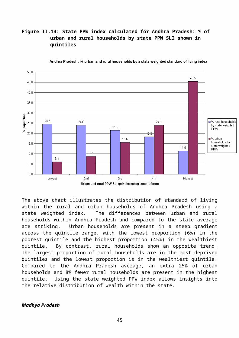
The above chart illustrates the distribution of standard of living within the rural households of Madhya Pradesh using two independent methods of calculation. Here, there are some differences between the two indices. The PPW index shows a gradient, with the higher proportions of Madhya Pradesh rural households in the lowest quintiles and the lowest proportions found in the highest quintiles. The NFHS index shows that the highest proportion of rural households in Madhya Pradesh are found in the middle quintile and the lowest proportions found in the two most extreme quintiles. What is consistent between the two indices is in finding the lowest proportion of rural households in the highest quintile.

The above indices calculated from All India data and using the NFHS methods show that most of the households in Madhya Pradesh are found in the poorer SLI quintiles and fewer are present in the highest quintile compared to the All India average.

Comparing Madhya Pradesh indices using correlationsThe Madhya Pradesh NFHS and state weighted PPW indices were compared using Pearson’s correlation coefficients. The correlation found was 0.96 (significant to the 0.01 level (two tailed).


36

Figure II.19: Scatter plot of Madhya Pradesh NFHS and state weighted PPW SLI


Comparison within Madhya Pradesh state PPW indexThe Madhya Pradesh state weighted SLI provides a comprehensive reflection of the socio-economic differentials within the state. Below, it is divided by Madhya Pradesh overall referent quintiles, allowing for a comparison between rural and urban households and the Madhya Pradesh average SLI distribution.

37

Figure II.20: State PPW index calculated for Madhya Pradesh: % of urban and rural households by state PPW SLI shown in quintiles

The above chart illustrates the distribution of standard of living within the rural and urban households of Madhya Pradesh using a state weighted index. There is a striking difference between the SLI distribution in urban and rural households. Rural households are present in a gradient across the quintile range, with the lowest proportion (10%) in the highest quintile and the highest proportion (25%) in the second poorest quintile. Urban households in Madhya Pradesh are distributed in an opposite and steep gradient. The highest proportion of urban households is found in the highest quintile and the lowest proportions found in the poorer two quintiles.

Using the state weighted PPW index allows insights into the relative distribution of wealth compared to the state average. It is apparent that rural households are disproportionately present in the poorest quintiles compared to urban households, which are over-represented in the wealthiest quintile.

OrissaThree forms of standard of living indices were calculated for Orissa: three All India weighted PPW indices (overall, rural, urban), a state weighted PPW index and an NFHS index (see Appendix for weightings).

Comparing Orissa and All India indices using correlationsThe Orissa NFHS and All India weighted PPW indices were compared Pearson’s correlation coefficients. The correlation found was 0.97 (significant to the 0.01 level (two tailed).

38


Figure II.21: Scatter plot of Orissa NFHS and All India weighted PPW SLI


Comparison between Orissa standard of living indices All of the standard of living indices were divided by referent quintiles using NFHS-2 All India data to establish the quintile cut-offs. Below, the NFHS index is compared to the PPW index by presenting the data in quintile form. The percentage of households in each SLI referent quintile is shown providing a comparison between the two indices and also with the All India average. The lowest quintile represents the most deprived households.

39

Figure II.22: All India overall indices calculated for Orissa: % of households by NFHS and PPW SLI shown in quintiles

The above chart illustrates the distribution of standard of living within the state of Orissa using two independent methods of calculation. The differences between the NFHS and PPW methods of calculating standard of living are relatively small. Both indices show a similar trend: a striking gradient along the quintile range, with the largest proportion of Orissa households present in the poorest quintile and a very small proportion in the wealthiest quintile. Compared to the All India average, Orissa has between 16-21% more households in the lowest quintile and about 10% fewer households in the wealthiest quintile.

40

Figure II.23: All India urban indices calculated for Orissa: % of urban households by NFHS and PPW SLI shown in quintiles

The above chart illustrates the distribution of standard of living within the urban households of Orissa using two independent methods of calculation. The differences between the NFHS and PPW methods of calculating standard of living are relatively small, with similar variations occurring across the quintile range. Both indices show the largest proportions of Orissa households in the lowest quintile, with the other four quintiles containing similar proportions of households. Furthermore, compared to the All India sample, Orissa has 13-19% more of its urban households in the most deprived quintile and fewer households in the other four quintiles.

41

Figure II.24: All India rural indices calculated for Orissa: % of rural households by NFHS and PPW SLI shown in quintiles

The above chart illustrates the distribution of standard of living within the rural households of Orissa using two independent methods of calculation. The differences between the NFHS and PPW methods of calculating standard of living are relatively small. Both indices show a similar trend: a striking gradient along the quintile range, with the largest proportion of Orissa rural households present in the poorest quintile and a very small proportion in the wealthiest quintile. Compared to the All India average, Orissa has between 12-17% more households in the lowest quintile and about 7% fewer households in the wealthiest quintile.

The above indices calculated from All India data and using the NFHS methods show that most of the households in Orissa are found in the poorest SLI quintiles compared to the All India average. This was true for both rural and urban households in Orissa when they were observed independently.

Comparing Orissa state indices using correlationsThe Orissa NFHS and state weighted PPW indices were compared Pearson’s correlation coefficients. The correlation found was 0.96 (significant to the 0.01 level (two tailed).

42


Figure II.25: Scatter plot of Orissa NFHS and state weighted PPW SLI


Comparison within Orissa state PPW indexThe Orissa state weighted SLI provides a comprehensive reflection of the socio-economic differentials within the state. Below, it is divided by Orissa overall referent quintiles, allowing for a comparison between rural and urban households and the Orissa average SLI distribution.

43

Figure II.26: State PPW index calculated for Orissa: % of urban and rural households by state PPW SLI shown in quintiles

The above chart illustrates the distribution of standard of living within the rural and urban households of Orissa using a state weighted index. There is a striking difference between the SLI distribution in urban and rural households. Rural households are predominantly found in the highest quintile (31%) with the lower proportions in the other four quintiles. Urban households in Orissa are distributed in a contrasting manner, with a huge proportion (53%) in the wealthiest quintile. The lowest proportion of urban households is in the second to lowest quintile.

Using the state weighted PPW index allows insights into the relative distribution of wealth within the state. Compared to the Orissa average, rural households are disproportionately present in the poorest quintile and urban households are over-represented in the highest quintile.

West BengalThree forms of standard of living indices were calculated for West Bengal: three All India weighted PPW indices (overall, rural, urban), a state weighted PPW index and an NFHS index (see Appendix for weightings).

Comparing West Bengal and All India indices using correlationsThe West Bengal NFHS and All India weighted PPW indices were compared Pearson’s correlation coefficients. The correlation found was 0.96 (significant to the 0.01 level (two tailed).


44

Figure II.27: Scatter plot of West Bengal NFHS and All India weighted PPW SLI


Comparison between West Bengal standard of living indices All of the standard of living indices were divided by referent quintiles using NFHS-2 All India data to establish the quintile cut-offs. Below, the NFHS index is compared to the PPW index by presenting the data in quintile form. The percentage of households in each SLI referent quintile is shown providing a comparison between the two indices and also with the All India average. The lowest quintile represents the most deprived households.

45

Figure II.28: All India overall indices calculated for West Bengal: % of households by NFHS and PPW SLI shown in quintiles

The above chart illustrates the distribution of standard of living within the state of West Bengal using two independent methods of calculation. The differences between the NFHS and PPW methods of calculating standard of living are relatively small. Both indices show a similar trend: a larger proportion of the West Bengal population is present in the lower standard of living quintiles. In both indices, the lowest proportions of households are present in the highest quintiles. Compared with the All India sample, both indices show that West Bengal has larger proportions of households in the lowest quintile and lower than average proportions in the highest two quintiles.

46

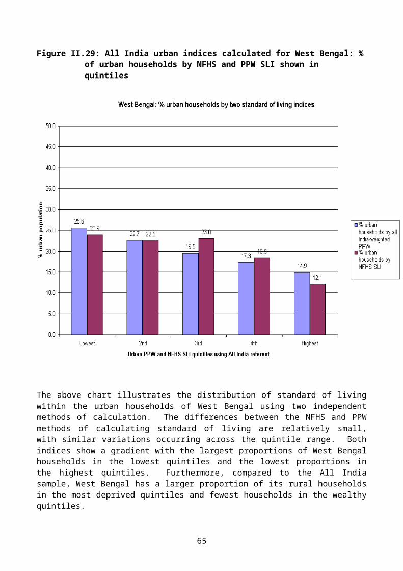
Figure II.29: All India urban indices calculated for West Bengal: % of urban households by NFHS and PPW SLI shown in quintiles

The above chart illustrates the distribution of standard of living within the urban households of West Bengal using two independent methods of calculation. The differences between the NFHS and PPW methods of calculating standard of living are relatively small, with similar variations occurring across the quintile range. Both indices show a gradient with the largest proportions of West Bengal households in the lowest quintiles and the lowest proportions in the highest quintiles. Furthermore, compared to the All India sample, West Bengal has a larger proportion of its rural households in the most deprived quintiles and fewest households in the wealthy quintiles.

47

Figure II.30: All India rural indices calculated for West Bengal: % of rural households by NFHS and PPW SLI shown in quintiles

The above chart illustrates the distribution of standard of living within the rural households of West Bengal using two independent methods of calculation. The differences between the NFHS and PPW methods of calculating standard of living are relatively small, with similar variations occurring across the quintile range. Both indices show that the largest proportion of the rural population is present in the lowest standard of living quintile. With both indices, the lowest proportion of households is present in the wealthiest quintile. Furthermore, compared to the All India sample, West Bengal has a larger proportion of its rural households in the most deprived quintile.

The above indices calculated from All India data and using the NFHS methods show that most of the households in West Bengal are found in the poorest SLI quintiles compared to the All India average. This was true for both rural and urban households in West Bengal when they were observed independently.

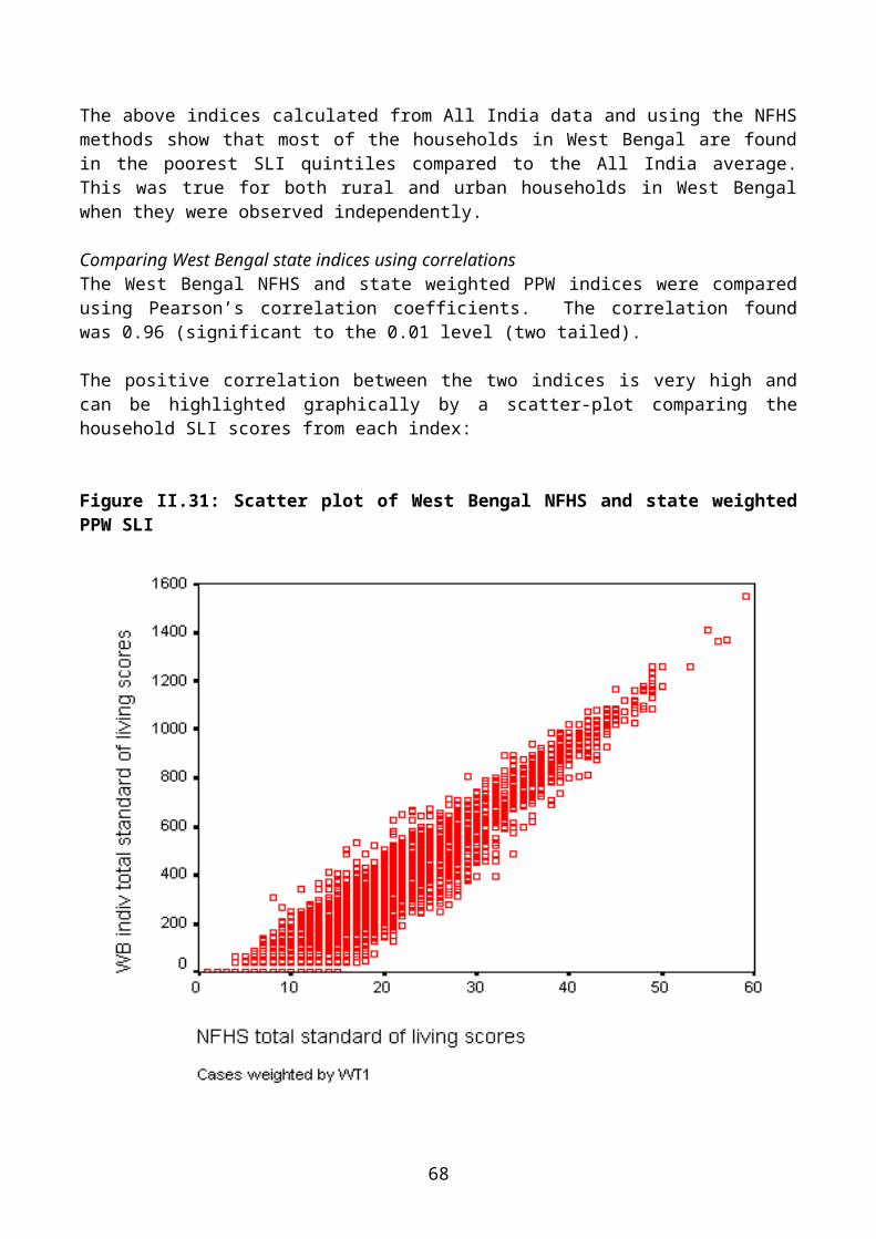
Comparing West Bengal state indices using correlationsThe West Bengal NFHS and state weighted PPW indices were compared using Pearson’s correlation coefficients. The correlation found was 0.96 (significant to the 0.01 level (two tailed).

48


Figure II.31: Scatter plot of West Bengal NFHS and state weighted PPW SLI


Comparison within West Bengal state PPW indexThe West Bengal state weighted SLI provides a comprehensive reflection of the socio-economic differentials within the state. Below, it is divided by West Bengal overall referent quintiles, allowing for a comparison between rural and urban households and the West Bengal average SLI distribution.

49

Figure II.32: State PPW index calculated for West Bengal: % of urban and rural households by state PPW SLI shown in quintiles

The above chart illustrates the distribution of standard of living within the rural and urban households of West Bengal using a state weighted index. The differences between urban and rural households within West Bengal - and compared to the state average - are striking. Urban households are present in a steep gradient across the quintile range, with the lowest proportion (5%) in the poorest quintile and the highest proportion (49%) in the wealthiest quintile. By contrast, rural households show an opposite trend. The largest proportion of rural households is in the most deprived quintiles and the lowest proportion is in the wealthiest quintile (10%). Compared to the West Bengal average, there are more rural households found in poor quintiles and more urban households in the higher quintiles.

50

Comparing the SLI distribution between the four states

Radar diagramsThe All India PPW index was calculated for each state and divided into All India referent quintiles. Below, the SLI distribution within each state is shown in radar diagrams whereby the All India average for each quintile is represented by the 20th percentile line. This allows for comparisons between states:

Figure II.33: Radar diagrams: All India overall PPW index for each state

These diagrams show that, compared to the other states, Orissa has a more deprived household population with the largest proportion in the lowest quintile and the smallest proportion in the highest quintile. West Bengal has a similar distribution to Orissa between the lowest and highest quintile. The household populations of Madhya Pradesh and Andhra Pradesh are the most evenly distributed across the quintile range.

51

Figure II.34: Radar diagrams: All India rural PPW index for each state

Compared to the other states, the rural household population of Andhra Pradesh is relatively evenly distributed across the quintile range. Orissa and West Bengal have comparatively fewer households in the higher quintiles and a large proportion of rural households in the most deprived quintile. This is particularly exaggerated for Orissa where over 56% are in the lowest two quintiles. The rural households of Madhya Pradesh are slightly skewed toward the more deprived quintiles, though not as severely as West Bengal or Orissa.

52

Figure II.35: Radar diagrams: All India urban PPW index for each state

Compared to the other states, Orissa urban households are predominantly found in the most deprived quintile, with fewer households than the All India urban average in the highest quintiles. West Bengal and Andhra Pradesh also have a high proportion of urban households in the first and second quintiles. The index is comparatively evenly distributed amongst Madhya Pradesh urban households, though the largest proportion is found in the most deprived quintile.

53

Gini coefficient based on the PPW standard of living index The Gini coefficient is a measure of inequality typically used to describe the distribution of income within a population. The coefficient ranges between 0 and 1, where 0 represents the most equal distribution of wealth, with everyone having an equal share, and 1 represents the most un-equal distribution, with one person having all the wealth.

The simplest and most intuitive interpretation of the Gini Coefficient is:

“If we choose two people at random from the income distribution, and express the difference between their incomes as a proportion of the average income, then this difference turns out to be (on average) twice the Gini Coefficient: a coefficient of 0.3 means that the expected difference between two people chosen at random is 60 per cent (2 x 0.3) of the average income. If the Gini Coefficient is 0.5 then the expected difference would be the average income itself.” (Raskall & Matherson, 1992)

Figure II.36: Example showing the line of equally distributed SLI across the population

This example shows the theoretical line of total equality, where the bottom 1% receives 1% of the total standard of living, the bottom 20% receives 20% of the total SLI, and so on.

54

Figure II.37: Example showing the likely distribution of SLI in a population

The above graph is an example of the likely distribution of SLI within a population. The Lorenz curve plots the proportion of total income held by each proportion of the population. The Gini coefficient is the ratio of the area between the two lines (i.e. the shaded area of the above graph) to the total area under the line of equality (e.g. the 45-degree line). If income become more unequally distributed, the Lorenz curve bulges further away from the complete equality line and the area between the curve and the 45-degree line increases. Thus the Gini coefficient rises with rising inequality and falls with falling inequality (see Goodman & Webb, 1994 for discussion).

55

The All India SLI Gini coefficientUsing the ‘Povcal’ program created by the World Bank, a Gini coefficient was calculated using the All India PPW SLI.

Figure II.38: The All India SLI Lorenz curve and Gini coefficient

Figure II.38 shows that India as a whole has a Gini coefficient of 0.49, this means that on average two Indian households selected at random will differ in standard of living by almost the average level living standards of the country. Although it is apparent from the above figure that inequalities in the distribution of SLI persist along the social gradient in India, more can be learnt by comparing SLI Gini coefficients calculated for each state to the All India SLI Gini.

56

Figure II.39: The four state SLI Lorenz curves and Gini coefficients compared to each other and to the All India SLI Lorenz curve and Gini

The All India Gini coefficient is 0.49 and is compared above to that of the four states. These results indicate that, with the exception of Andhra Pradesh, the three other states have greater levels of inequality than the All India average. The Gini coefficient for Orissa is highest (0.59), indicating that the distribution of SLI within the state is more unequal than for the other three states - and All India. The Gini for Andhra Pradesh is closest to the All India average (0.48), whereas Madhya Pradesh and West Bengal have similar coefficients, both of which indicate greater levels of inequality than Andhra Pradesh or the All India average.

57

Summary of comparison between the standard of living indicesThe two independent standard of living indices have been compared and found to be both reliable and very similar. The correlations at the All India level as well as at the state level have been consistently high, with about 90% of the variance being explained by the association.

The All India PPW index allows for comparisons between states, using both the All India possessions weightings and the All India referent quintile cut-off points. This means that the states can be compared with each other as well as with the All India average through the use of objective and scientific measurements. It was found that Orissa had the highest proportion of households in the poorest SLI quintile (between 36-41%), followed by West Bengal, which also had large proportions of its households in the lowest quintile (between 27-29%). Andhra Pradesh and Madhya Pradesh had more even distributions across the quintile range, not dissimilar to the All Indian average.

The state weighted PPW indices, calculated for each state independently using its own proportionate possessions weighting, allows for a representation of relative wealth within the state. This was shown when the standard of living of urban and rural household were compared. Within each state, it was found that a disproportionately high proportion of rural households are found in the most deprived SLI quintiles, whereas urban households are over-represented in the wealthier SLI quintiles, compared to the state average.

From the analyses above, it can be concluded that the two indices show similar trends for All India, as well as for the individual states. It is apparent that Orissa is more severely deprived compared to the All India average, as well as compared to the other three states, with large proportions of its households being in the poorest standard of living quintile. Furthermore, all of the states observed here at the state level show important disparities between the urban and rural environments, with a disproportionate prevalence of rural households in the lowest SLI quintile.

Calculating Gini coefficients, based on the distribution of SLI within the All India sample population and the state sample populations, confirms the trends seen across the SLI quintiles. The All India population has significant socio-economic inequalities along the social gradient, reflected by the SLI Gini coefficient of 0.49. When comparisons are made between the various Gini coefficients, it becomes apparent that Orissa has the most unequal distribution of wealth out of the four states and All India, with a coefficient of 0.59. Orissa’s poorly distributed wealth is closely followed by West Bengal (0.54) and Madhya Pradesh (0.53). Andhra Pradesh has a similar SLI distribution to All India , with a slightly better coefficient (0.48).

58

SECTION III

ANTHROPOMETRY, CHILD HEALTH AND STANDARD OF LIVING

All India PPW and NFHS SLI compared to child health outcomesAn individual’s health is closely associated with their socio-economic position. Anthropometric measurements are used as proxy measures of health and nutritional status alongside morbidity and immunisation. An assessment of the associations between each index and child health outcome measures was carried out in order to compare the two methods of calculating standard of living.

The first method used to compare the indices was to create a ‘relative index of inequality’ (RII). This was used to represent the disparities in child health along the social gradient. There are only slight differences between the respective RII for each SLI, primarily due to the different methods used to calculate the index.

The differences were then further explored by comparing the distribution of each child health outcome by SLI quintiles. Overall, the child health outcome proportions in each quintile group were similar for the two indices. The NFHS index tended to have a higher proportion of children in the lower quintiles and a lower proportion in the high quintiles. The PPW index tends to capture more individuals with a higher standard of living. This means that the gradient difference between low and high standard of living will be steeper for the NFHS SLI and more attenuated for the PPW SLI.

Finally, using the results from univariate logistic regression analyses between child health outcomes and SLI, a comparison was made between the odds ratios of each quintile group for the two indices. Differences were small and for some child health outcomes more than others. Overall, the trends and results were the same for both indices.

Relative Index of Inequality (RII)How the relative index of inequality was calculated:

Each standard of living index was divided into population quintiles. Each group was given a score between 0 and 1 according to the proportion of households

with a higher position than the midpoint of each group within this hierarchy. The new numerical indicators of socio-economic position (SEP) are then related to health

outcomes through a regression analysis. This yields the Relative Index of Inequality for a specific health outcome. The RII for diarrhoea is therefore the Odds Ratio of having diarrhoea at the top compared to the bottom of the socio-economic hierarchy. The larger the RII, the greater the degree of inequality.

59

Health outcome measures used:

Incidence of diarrhoea Stunted Underweight Wasted Severely stunted Severely underweight Severely wasted Moderate anthropometric failure Severe anthropometric failure Immunised for measles

Comparing standard of living to child health outcomes using a Relative Index of Inequality (RII)

Incidence of diarrhoea

Table III.1: Diarrhoea – whether child had diarrhoea within the last two weeks

Count Valid %No report of diarrhoea 24785 81Had diarrhoea in past two weeks 5802 19Total 30587 100

RII for diarrhoea using the PPW SLI Odds ratio1.2*

95% CI1.1-1.3

RII for diarrhoea using NFHS SLI*P<0.001 1.3* 1.2-1.4

The RII is represented in this analysis by the odds ratio. The RII based on the PPW SLI shows that children with the lowest standard of living are 20% more likely to have had diarrhoea recently than those with the highest. The RII based on the NFHS SLI shows that children with the lowest SLI are 30% more likely to have had diarrhoea recently than those with the highest.

Figure III.1: Proportion of children with diarrhoea by SLI quintile using two indices

60

This bar chart shows the total percentage of children with diarrhoea per quintile group for both standard of living indices. Both indices have a similar distribution of proportions in each quintile. The lowest proportions of children with diarrhoea are found in the wealthiest quintile for both indices.

61

Figure III.2: Two logistic regression analyses with diarrhoea as dependent variable, and each SLI as categorical independent variables with highest quintile as referent

This chart shows the change in odds ratio from the lowest to the fourth SLI quintile groups with the 95% confidence intervals represented by the bars. Again, this figure shows that the two indices find similar results. There are minor differences in diarrhoea prevalence along the social gradient.

62

Stunting (height for age)

Table III.1: Stunting – whether child is stunted

Count Valid %Not stunted 13372 55Stunted 11024 45Total 24396 100RII for Stunting using the PPW SLI Odds ratio

3.9*95% CI3.6-4.3

RII for Stunting using the NFHS SLI*P<0.001

3.9* 3.6-4.3

The RII is represented in this analysis by the odds ratio. The RII based on the PPW SLI shows that children with the lowest standard of living are nearly four times more likely to be stunted than those with the highest SLI. The relative index of inequality based on the NFHS SLI shows that children with the lowest standard of living are also nearly four times more likely to be stunted than those with the highest SLI.

Figure III.3: Proportion of children with stunting by SLI quintile using two indices

63

This bar chart shows the total percentage of stunted children per quintile group for both standard of living indices. Both indices have a similar distribution of proportions in each quintile and show the same downward trend from lowest to highest quintile. The largest proportions of children with stunting are found in the poorest SLI quintiles. The lowest proportion of children with stunting is found in the wealthier households.

Figure III.4: Two logistic regression analyses with stunting as the dependent variable and each SLI as categorical independent variables with highest quintile as referent

This chart shows the change in odds ratio from the lowest to the fourth SLI quintile groups with the 95% confidence intervals represented by the bars. There are small differences between the two indices but, overall, they both show the same trend. A negative gradient persists along the SLI range with the children in lower standard of living quintiles having higher odds of being stunted compared to the 5th (highest) referent quintile.

64

Underweight (weight for age)

Table III.3: Children underweight

Count Valid %Not Underweight 12903 53Underweight 11493 47Total 24396 100RII for Underweight using the PPW SLI Odds ratio

4.8*95% CI4.4-5.3

RII for Underweight using the NFHS SLI*P<0.001

4.9* 4.5-5.4

The RII is represented in this analysis by the odds ratio. The RII based on the PPW SLI shows that children with the lowest standard of living are nearly five times more likely to be underweight than those with the highest SLI. The relative index of inequality based on the NFHS SLI shows that children with the lowest standard of living are also nearly five times more likely to be underweight than those with the highest SLI.

Figure III.5: Proportion of underweight children by SLI quintile using two indices

65

This bar chart shows the total percentage of underweight children per quintile group for both standard of living indices. Both indices have a similar distribution of proportions in each quintile and show the same downward trend from lowest to highest quintile. Larger proportions of underweight children are present in the poorer quintiles, with the lowest prevalence of underweight found in the wealthiest quintile.

Figure III.6: Two logistic regression analyses with underweight as the dependent variable and each SLI as categorical independent variables with highest quintile as referent

This chart shows the change in odds ratio from the lowest to the fourth SLI quintile groups with the 95% confidence intervals represented by bars. There are slight differences between the two indices, with overall indicate the same trend. There is a negative gradient whereby children in lower standard of living quintiles having higher odds of being underweight compared to the 5th (highest) referent quintile.

66

Wasting (weight for height)

Table III.4: Children wasted

Count Valid %Not Wasted 20651 84Wasted 3904 16Total 24555 100RII for Wasted using the PPW SLI Odds ratio

2.7*95% CI2.4-3.1

RII for Wasted using the NFHS SLI*P<0.001

2.9* 2.6-3.3

The RII is represented in this analysis by the odds ratio. The RII based on the PPW SLI shows that children with the lowest standard of living are over two-and-a-half times more likely to be wasted than those with the highest SLI. The relative index of inequality based on the NFHS SLI shows that children with the lowest standard of living are nearly three times more likely to be wasted than those with the highest SLI.Figure III.7: Proportion of wasted children by SLI quintile using two indices

67

This bar chart shows the total percentage of wasted children per quintile group for both standard of living indices. Both indices have a similar distribution of proportions in each quintile and show the same downward trend from lowest to highest quintile. The indication here is that few children in the wealthier households suffer from wasting, whereas higher proportions of wasted children are found in the poorer SLI quintiles.

Figure III.8: Two logistic regression analyses with wasting as the dependent variable and each SLI as categorical independent variables with highest quintile as referent

This chart shows the change in odds ratio from the lowest to the fourth SLI quintile groups with the 95% confidence intervals represented by bars. The two indices show the same negative trend. Children from more deprived households have significantly higher odds of being wasted than those from the wealthiest quintile.

68

Severely stunted

Table III.5: Children severely stunted

Count Valid %Not Severely stunted 18838 77Severely stunted 5557 23Total 24396 100RII for Severely stunted using the PPW SLI Odds ratio

4.3*95% CI3.9-4.8

RII for Severely stunted using the NFHS SLI*P<0.001

4.5* 4.0-5.1

The RII is represented in this analysis by the odds ratio. The RII based on the PPW SLI shows that children with the lowest standard of living are more than four times more likely to be severely stunted than those with the highest SLI. The relative index of inequality based on the NFHS SLI shows that children with the lowest standard of living are four-and-a-half times more likely to have been severely stunted than those with the highest SLI.

69

Figure III.9: Proportion of severely stunted children by SLI quintile using two indices

This bar chart shows the total percentage of severely stunted children per quintile group for both standard of living indices. Both indices have a similar distribution of proportions in each quintile and show the same downward trend from lowest to highest quintile. Severely stunted children are predominantly found in the lower SLI quintiles, whilst lower proportions are present in the wealthier households.

70

Figure III.10: Two logistic regression analyses with severe stunting as the dependent variable and each SLI as categorical independent variables with highest quintile as referent

This chart shows the change in odds ratio from the lowest to the fourth SLI quintile groups with the 95% confidence intervals represented by bars. There are slight differences between the two indices, with the NFHS index having consistently higher odds along the quintile distribution. Both indices show a similar negative gradient whereby the children in lower standard of living quintiles have significantly higher odds of being severely stunted compared to the 5th (highest) referent quintile.

71

Severely underweight

Table III.6: Children severely underweight

Count Valid %Not Underweight 20030 82Severely stunted 4366 18Total 24396 100RII for Severely underweight using the PPW SLI Odds ratio

6.2*95% CI5.5-7.1

RII for Severely underweight using the NFHS SLI*P<0.001

6.7* 5.9-7.6

The RII is represented in this analysis by the odds ratio. The RII based on the PPW SLI shows that children with the lowest standard of living are more than six times more likely to be severely underweight than those with the highest SLI. The relative index of inequality based on the NFHS SLI shows that children with the lowest standard of living are nearly seven times more likely to be severely underweight than those with the highest SLI.

72

Figure III.11: Proportion of severely underweight children by SLI quintile using two indices

This bar chart shows the total percentage of severely underweight children per quintile group for both standard of living indices. Both indices have a similar distribution of proportions in each quintile and show the same downward trend from lowest to highest quintile. This chart indicates that smaller proportions of severely underweight children are found in the wealthiest quintiles, whilst the highest proportions are found in the lowest quintile.

73

Figure III.12: Two logistic regression analyses with severely underweight as the dependent variable and each SLI as categorical independent variables with highest quintile as referent

This chart shows the change in odds ratio from the lowest to the fourth SLI quintile groups with the 95% confidence intervals represented by bars. Both indices show the same striking gradient. Indeed, children in the lowest quintile are between 5.7 and 4.9 times more likely to be severely stunted than those in the highest quintile. The two indices indicate that severe stunting is highly socially patterned.

74

Severely wasted

Table III.7: Children severely wasted

Count Valid %Not Severely wasted 23840 97Severely wasted 716 3Total 24555 100RII for Severely wasted using the PPW SLI Odds ratio

3.7*95% CI2.8-4.9

RII for Severely wasted using the NFHS SLI*P<0.001

3.8* 2.9-5.1

The RII is represented in this analysis by the odds ratio. The RII based on the PPW SLI shows that children with the lowest standard of living are more than three-and-a-half times more likely to be severely wasted than those with the highest SLI. The relative index of inequality based on the NFHS SLI shows that children with the lowest standard of living are nearly four times more likely to be severely wasted than those with the highest SLI.

75

Figure III.13: Proportion of severely wasted children by SLI quintile using two indices

This bar chart shows the total percentage of severely wasted children per quintile group for both standard of living indices. The indices have varying distributions of proportions in each quintile, probably due to the small numbers of severely wasted children. The proportions of severely wasted children are much lower than for the other anthropometric measures.

76

Figure III.14: Two logistic regression analyses with severely wasted as the dependent variable and each SLI as categorical independent variables with highest quintile as referent

This chart shows the change in odds ratio from the lowest to the fourth SLI quintile groups with the 95% confidence intervals represented by bars. The regression analysis provides more information on the relationship between severe wasting and standard of living than the bar chart. Here, both indices show a negative gradient, whereby children in the lower quintiles have significantly higher odds of being wasted compared to the 5th (highest) referent quintile.

77

Moderate anthropometric failure: a composite measure combining stunting, wasting and underweight

Table III.8: Children suffering moderate anthropometric failure

Count Valid %No moderate anthropometric failure 9806 40Moderate anthropometric failure 14590 60Total 24396 100RII for moderate anthropometric failure using the PPW SLI

Odds ratio4.6*

95% CI4.2-5.1

RII for moderate anthropometric failure using the NFHS SLI*P<0.001

4.7* 4.2-5.2

The RII is represented in this analysis by the odds ratio. The RII based on the PPW SLI shows that children with the lowest standard of living are more than four-and-a-half times more likely to have moderate anthropometric failure than those with the highest SLI. The relative index of inequality based on the NFHS SLI shows that children with the lowest standard of living are nearly five times more likely to have moderate anthropometric failure than those with the highest SLI.

78

Figure III.15: Proportion of children with moderate anthropometric failure by SLI quintile using two indices

This bar chart shows the total percentage of children with moderate anthropometric failure per quintile group for both standard of living indices. Both indices have a similar distribution of proportions in each quintile and show the same downward trend from lowest to highest quintile. The chart indicates that anthropometric failure is socially patterned with the lowest proportion of children with moderate anthropometric failure in the highest quintile and the highest proportions in the lower quintiles.

79

Figure III.16: Two logistic regression analyses with moderate anthropometric failure as the dependent variable and each SLI as categorical independent variables with highest quintile as referent

This chart shows the change in odds ratio from the lowest to the fourth SLI quintile groups with the 95% confidence intervals represented by bars. Again, the two indices show a similar negative gradient: the children in lower standard of living quintiles having higher odds of being having moderate anthropometric failure compared to the 5th (highest) referent quintile.

80

Severe anthropometric failure: a composite measure combining stunting, wasting and underweight

Table III.9: Children suffering severe anthropometric failure

Count Valid %No severe anthropometric failure 17291 71Severe anthropometric failure 7105 29Total 24396 100RII for severe anthropometric failure using the PPW SLI

Odds ratio5.0*

95% CI4.5-5.6

RII for severe anthropometric failure using the NFHS SLI*P<0.001

5.2* 4.7-5.8

The RII is represented in this analysis by the odds ratio. The RII based on the PPW SLI shows that children with the lowest standard of living are five times more likely to have severe anthropometric failure than those with the highest SLI. The relative index of inequality based on the NFHS SLI shows that children with the lowest standard of living are more than five times more likely to have severe anthropometric failure than those with the highest SLI.

81

Figure III.17: Proportion of children with severe anthropometric failure by SLI quintile using two indices

This bar chart shows the total percentage of children with severe anthropometric failure per quintile group for both standard of living indices. Both indices have a similar distribution of proportions in each quintile and show the same downward trend from lowest to highest quintile. The lowest proportion of children with severe anthropometric failure is in the wealthiest quintile and the highest proportions are found in the lowest two quintiles.

82

Figure III.18: Two logistic regression analyses with severe anthropometric failure as the dependent variable and each SLI as categorical independent variables with highest quintile as referent

This chart shows the change in odds ratio from the lowest to the fourth SLI quintile groups with the 95% confidence intervals represented by bars. Both indices show that severe anthropometric failure is socially patterned, with a negative gradient apparent in the odds ratios along the SLI range. The children in lower standard of living quintiles have significantly higher odds of having severe anthropometric failure compared to the 5th (highest) referent quintile.

83

Measles Immunisation: Children aged between 12 and 34 months only

Table III.10: Children not immunised

Count Valid %Not immunised against measles 8388 46Immunised against measles 10012 54Total 18401 100RII for lack of measles immunisation using the PPW SLI

Odds ratio10.6*

95% CI9.4-11.8

RII for lack of measles immunisation using the NFHS SLI*P<0.001

9.7* 8.6-10.9

The RII based on the PPW SLI shows that children with the lowest standard of living are more than ten-and-a-half times more likely to have not been immunised for measles than those with the highest SLI. The relative index of inequality based on the NFHS SLI shows that children with the lowest standard of living are nearly ten times more likely to have not been immunised for measles than those with the highest SLI.

84

Figure III.19: Proportion of children not immunised against measles by SLI quintile using two indices

This bar chart shows the total percentage of children not immunised for measles per quintile group for both standard of living indices. Both indices have a similar distribution of proportions in each quintile and show the same downward trend from lowest to highest quintile. The proportion of children not immunised for measles is highest in the poorest quintiles and lowest in the wealthiest quintile.

85

Figure III.20: Two logistic regression analyses not immunised for measles as the dependent variable and each SLI as categorical independent variables with highest quintile as referent

This chart shows the change in odds ratio from the lowest to the fourth SLI quintile groups with the 95% confidence intervals represented by bars. Both indices show the striking gradient along the SLI quintile range. Indeed, the change in odds ratio from the lowest SLI quintile to the highest suggests that measles immunisation is highly socially patterned. The children in lower standard of living quintiles have significantly higher odds of not being immunised for measles compared to the 5 th (highest) referent quintile.

86

Summary of comparison between the two indicesThe proportionate possessions weighting (PPW) provides a comparable measure of household standard of living to that created by the NFHS. It also has the advantage of being a more objective measure, as it uses a scientific method to calculate the weightings. Such an independent method could easily be used in other studies without requiring an extensive or in-depth knowledge of local socio-economic conditions. In addition, it enables an assessment of relative poverty at different levels (regional, state, national, and international), which the NFHS SLI does not.

More importantly, the findings suggest that significant inequalities persist along the socio-economic gradient in India. The measures of anthropometric failure show particularly strong differences in the health and nutritional status of children from low standard of living households compared to those from high standard of living households. The analyses using measles immunisation as the outcome measure indicate huge disparities in access to services, such as child immunisation, depending on relative standard of living. Prevalence of diarrhoea did not change substantially along the SLI quintile range, whereas outcomes such as underweight, severe stunting, anthropometric failure and measles immunisation showed a consistent gradient whereby the children in the more deprived SLI quintiles had significantly higher odds of a poor health outcome than those in the highest quintile.

Such results indicate substantial inequalities in health and access to health services along the socio-economic gradient, here measured by two independent standard of living indices. The findings show both chronic and acute health outcomes being strongly socially patterned in this All India sample.

87

SECTION IV

AREA FACILITY INDEX

Introduction‘Area standard of living’ has at least three different meanings (Macintyre et al, 1993; Macintyre, 1997):

1. A compositional meaning, whereby an area is considered to be deprived if it contains a large number of poor people. In this case, the spatial effects are entirely due to the concentration of poor people in a given area – there are no independent area effects (Slogget and Joshi, 1994; Dale, 1997).

2. A collective meaning, whereby an area is considered to be deprived because, if it contains a lot of poor people, a ‘social miasma’ may exist. That is, a concentration of poor people will exert a collective influence, above and beyond their individual circumstances. For example, it may be difficult to find a job if you live in a deprived area because employers are prejudiced against people from poor areas. Although this is a commonly held belief, there is relatively little (other than anecdotal) evidence to support it (Brown and Madge, 1982).

3. A public goods or environmental meaning, whereby an area is considered deprived because it lacks facilities (roads, hospitals, schools, libraries, etc.) or because it suffers from high pollution levels (Bramley, 1997).

These three meanings of area deprivation are separate and distinct but are often confused. (Lee et al, 1995).

Area Facility IndexAlthough household standard of living has been assessed using two different methods of calculation, a household with a high standard of living may be situated in a deprived area with poor access to basic facilities such as clean water and health care. In order to establish relative standard of living based on public access facilities, an Area Facility Index was created for rural areas based on the NFHS-2 All India Village data set.

Sixteen different public health facilities were used as markers for the index. They can be broken down into markers of distance and markers of availability.

Distance from facilitiesThe distance markers were weighted on a scale from 0 to 2. A score of 2 was attributed if the distance of the village from the marker was between 0 and 2 kilometres. A score of 1 was given if the distance was between three and 20 kilometres and a score of 0 was given if the distance was greater than 20 kilometres. The distance markers used are: distance to nearest town, district headquarters, railway station, transport service, primary school, higher education centre, primary health centre, secondary health centre, post-office, telegraph-office, and bank.

88

Availability of facilitiesThe availability markers were weighted on a scale from 0 to 1. A score of 1 was attributed if the facility was present in the village and a score of 0 was given if the facility was not. Both drainage and electricity facilities were scored from 0 to 2. A score of 2 was given if the electricity supply was ‘regular’ or the drainage was ‘underground’, a score of 1 was given if the electricity supply was ‘irregular’ or the drainage was ‘open’ and a score of 0 was given if the facility was not available. The availability markers are: availability of a community television set, a weekly market, a market shop, drainage and electricity.

The Area Facility Index (AFI) is composed of various domains:

An education domain, consisting of distance to nearest primary school and distance to nearest higher education centre (middle school and secondary school and college).

A health domain, consisting of distance to primary health centre (primary health centre, community health centre, and dispensary) and distance to secondary health centre (government hospital, private clinic and private hospital).

A transport domain, consisting of distance to nearest railway station and to nearest transport service.

A communications and media domain, consisting of distance to nearest post-office, distance to nearest telegraph-office, availability of community television set.

A finance domain, consisting of distance to nearest bank. A commercial domain, consisting of availability of weekly market, and availability of

market shop. A general domain, consisting of distance to nearest town, and distance to district

headquarters.

The scores of each marker are added up to form an overall AFI. The index scores range from 0 to 29, in ascending order, from villages with the least access to facilities (0) to those with the best access to facilities (29).

When the household proportionate possessions SLI and the AFI are compared, using Pearson’s correlation, no association was found between the two (R2=0.00). This indicates that households across the entire standard of living distribution are present in areas of varying access to facilities. Put in simpler terms, poorer and wealthier households are present both in areas of good and bad access to facilities.

Comparisons between area and householdTo investigate the interactions between household standard of living and the area facilities index, analyses were run assessing the relationship of both indices with health outcomes. Three logistic regression models were constructed for each health outcome:

Univariate models, where each index was entered respectively as a continuous independent variable.

Multivariate models, where both indices were entered into the same model as continuous independent variables.

89

Multivariate models, where both indices were entered into the same model as continuous independent variables and an interaction variable (household index by AFI) was entered as an independent continuous variable.

Table IV.1: Univariate and Multivariate model results of the association between household standard of living and area facilities and anthropometric failure

Child health Univariate: Household SLI

Univariate: Area facilities index

Model: Household SLI and Area facilities index

Model: Household SLI, Area facilities index and interaction term between the two

SLI AFI SLI AFI SLI AFI Interaction term

Stunting 2.9 (2.6-3.3)* 1.1 (1.02-1.2)* 2.9 (2.6-3.2)* 1 (0.9-1.1)ns 1.8 (1.4-2.2)* 0.8 (0.7-0.9)* 1 (1.0-1.0)*

Wasting 2.7 (2.3-3.1)* 1.2 (1.09-1.4)* 2.6 (2.3-3.1)* 1.1 (1.02-1.3) ^ 2.5 (1.8-3.3)* 1.1 (0.9-1.3)ns 1 (1.0-1.0)ns

Underweight 3.7 (3.3-4.1)* 1.2 (1.1-1.3)* 3.6 (3.2-4.1)* 1.1 (1.02-1.2)* 1.9 (1.5-2.4)* 0.8 (0.7-0.9)* 1 (1.0-1.0)*

Stunting (sev) 2.9 (2.5-3.3)* 1.2 (1.06-1.3)* 2.9 (2.5-3.2)* 1.1 (0.9-1.2)ns 1.7 (1.3-2.2)* 0.8 (0.7-1.0)ns 1 (1.0-1.0)*

Wasting (sev) 3.6 (2.6-5.0)* 1.09 (0.8-1.4)* 3.6 (2.6-4.9)* 1 (0.7-1.3)ns 3.2 (1.7-6.3)* 0.9 (0.6-1.4)ns 1 (1.0-1.0)ns

Underweight (sev) 4.3 (3.7-5.0)* 1.2 (1.08-1.4)* 4.3 (3.7-4.9)* 1.1 (0.9-1.2)ns 2.5 (1.9-3.4)* 0.8 (0.7-1.0)ns 1 (1.0-1.0)*

Anth failure 1.8 (1.6-2.0)* 1.1 (1.08-1.2)* 1.8 (1.6-2.0)* 1.1 (1.0-1.2)* 1.1 (0.9-1.4)ns 0.9 (0.8-1.0)ns 1 (1.0-1.0)*

Anth failure (sev) 2.5 (2.3-2.8)* 1.2 (1.1-1.3)* 2.5 (2.2-2.8)* 1.1 (1.0-1.2)* 1.6 (1.3-2.0)* 0.9 (0.8-1.0)ns 1 (1.0-1.0)*

Maternal health services

SLI AFI SLI AFI SLI AFI Interaction term

Visited health facility in last 12 months

3.4 (3.0-3.7)* 1.4 (1.2-1.5)* 3.3 (3.0-3.7)* 1.2 (1.1-1.4)* 2.6 (2.1-3.2)* 1.1 (1.0-1.3)* 1 (1.0-1.)*

Went for antenatal care

1.5 (1.3-1.8)* 0.8 (0.6-0.9)^ 1.5 (1.3-1.8)* 0.7 (0.6-0.9)* 1.7 (1.2-2.5)* 0.8 (0.6-1.0)ns 1 (1.0-1.0)ns

Odds ratios (95% Confidence intervals)* P<0.01^P<0.05ns = not significant

The univariate results show that, in separate analyses, both household standard of living and area facilities are related to health outcomes. When both indices are simultaneously put into a multivariate model, the associations between health and area become attenuated whereas the associations between health and SLI remain the same. In a multivariate model where a further interaction term is added, there are virtually no associations between health and area facilities. The associations between household SLI and health are attenuated but remain consistent and significant.

90

These analyses show that, despite finding some associations between area facilities and health, household standard of living remains a stronger overall predictor of health outcomes.

Multi-Level ModelsHowever, it must be noted that the model described above is miss-specified as household standard of living and area facilities are measured at two different levels. In order to correctly assess the relative effects of these indices on ill health, it is necessary to use a hierarchal or multi-level model. These are discussed briefly below and in much greater detail in a separate report by Dr. S.V. Subramanian “Methodologies for analyzing socioeconomic and geographic disparities in health using the Indian National Family and Health Survey (INFHS): a multilevel statistical approach”

For reasons of cost and efficiency, the NFHS Survey adopted a multistage or clustered design. This involved four stages of sampling, all states were selected for survey, then within states a sample of primary sampling units (villages or urban neighbourhoods) were selected, then within these primary sampling units a sample of households were selected and then only certain individuals were interviewed in each household. Such a design generates a 4-level hierarchical structure with individuals at level 1 nested in households at level 2, which are in turn nested in villages or neighbourhoods at level 3, which in turn are located within specific states at level 4. Individuals living in the same household or village can be expected to be more alike than a random sample, that is they are autocorrelated, and consequently such clustered samples do not contain as much `information' as simple random samples of similar size.

Most conventional statistical analyses ignore this autocorrelation and this results in incorrect estimates of precision, standard errors, confidence limits and tests (Skinner et al, 1989). In the univariate and logistic regression results in this report there is a slightly increased risk of finding differences and relationships where none exist.

Multilevel analysis differs from conventional General Linear Model (GLM) analysis (e.g. logistic and linear regression, correlation, etc.) in that. the hierarchical structure is seen not as a result of multistage sampling, but rather the population itself is conceptualised to have a complex (often hierarchical) structure (Goldstein, 1987,199I, 1995, Jones 1997). Individuals, households, villages and states are seen as important structures in the population which may be measured and modelled. In the terminology of survey research, with multilevel models the standard errors are automatically adjusted for the design effect and associated autocorrelation or infra-class correlation that results from the hierarchical structure. However, multilevel analysis is more than just a technical improvement to GLM models, it also allows for the modelling of contextuality. Thus, such models are not only able to model between-individual variation (at level 1) and household variation (at level 2) but also between-place variation (between-village and between-state variation at levels 3 and 4 respectively).

Conventional GLM analysis has either been undertaken at the aggregate (e.g. village) level (as adopted by many geographers) or the individual (the preferred choice of many epidemiologists). Choosing to work at the aggregate level lays one open to the charge of the ecological fallacy (Robinson, 1950) and aggregation bias (Roberts and Burstein, 1980), while choosing to work at the individual level risks being found guilty of the atomistic fallacy (Alker, 1969). The latter approach misses the context in which individual behaviour occurs, while the former falls to recognise that it is individuals who act, not aggregates. Working at the individual level misses the context of local cultures, while working at the aggregate level fails to capture individual variation fully. The standard statistical approaches to

91

aggregate analysis (such as the calculation of rates and averages and regression modelling) and to dis-aggregate analysis (such as cross-tabulation, logistic and log-linear modelling) cannot deal with these problems because they operate at a single level. Clearly if we ignore any level in an analysis we can say nothing substantive about it (Jones, 1997).

Multilevel models were explicitly developed to resolve this dilemma by working at more than one level simultaneously, so that an overall model can handle the micro-scale of people and the macro-scale of places. Most importantly by distinguishing different levels, multilevel procedures allow relationships to vary according to context. This is explained in much greater detail in the following section.

92

Section V

A multilevel statistical approach to analysing socio-economic and geographic disparities in health

IntroductionOne methodology that has captured the imaginations of health researchers interested in simultaneously modelling individual and area variations in health are the multilevel statistical procedures (Goldstein, 2003), also known as hierarchical (Raudenbush and Bryk, 2002), mixed and random-effects (Laird and Ware, 1982), covariance components (Dempster et al., 1981) or random-coefficient regression (Longford, 1993) models. This report provides an introduction to these procedures from a conceptual as well as practical perspective and discussion is done within the context of utilizing and analysing the Indian National Family Health Survey (NFHS) data, which is the Indian equivalent of the wider Demographic and Health Surveys (DHS) currently underway in some 60 countries (WWW.MEASUREDHS.COM). Specific emphasis is placed on the modelling strategies that characterize multilevel statistical techniques along with their empirical interpretation. The report begins by introducing the idea of multilevel structures followed by conceptual outline of the nature of research questions that the multilevel framework can help us address, with particular emphasis on modelling contextual influences on health. The statistical implementation of the multilevel models to answering such questions will be the focus of the subsequent section. In the final section, the discussion is exemplified with a multilevel analysis of tobacco chewing-related behaviour and its relation to individual and area-based standard of living index (SLI).

Multilevel structuresMultilevel methods are specifically geared towards the statistical analysis of data that have a nested structure. The nesting, typically, but not always, is often seen in hierarchical terms. Figure V.I, for instance, shows a two level structure that is often present in the NFHS data such that there are many individuals at level-1 are nested within a smaller number of areas (representing villages/wards) at level-2. Importantly, such structures arise routinely in health and social sciences and indeed, “once you know that hierarchies exist, you see them everywhere”. The term multilevel, therefore, relates to the levels of analysis, which usually, but not always, consists of, individuals (at lower level) who are nested within spatial units (at higher levels). As will be discussed later, there are other data structures that can also be considered as a special case of multilevel structure.

Figure V. I: A two level hierarchical structure of individuals (at level-1) nested within villages (at level-2)

93

http://www.measuredhs.com/

Why should we be concerned about such nested structures, say individuals nested within areas? The existence of such nested data is neither random nor ignorable; for instance, individuals differ but so do areas. Differences among areas could either be directly due to the differences among individuals who live in them; or groupings based on areas may arise for reasons less strongly associated with the characteristics of the individuals who live in them. Regardless, once such groupings are established, even if their establishment is random, they will tend to become differentiated. This would imply that the group (e.g., areas) and its members (e.g., individual residents) can exert influence on each other suggesting different sources of variation (e.g., individual-induced and area-induced) in the outcome variable of interest and thus compelling analysts to consider covariates at the individual and at the area level.

Ignoring this multilevel structure of variations not simply risks overlooking the importance of area effects, but has implications for statistical validity (Aitkin and Longford, 1986). For instance, individuals within any one area, because they belong to a similar context, tend to be more alike (than different) in their health experiences. More formally, the individual samples are correlated or clustered. Such clustered samples do not contain as much information as simple random samples of similar size and ignoring this autocorrelation and clustering results in increased risk of finding differences and false positive relationships.

Clustered data may also arise as a result of sampling strategies. For instance, while planning large-scale survey data collection, such as the NFHS, for reasons of cost and efficiency, it is usual to adopt a multistage sampling design. For instance, the NFHS involved a three-stage design, with states being selected first, then villages/wards or groups of villages/wards (referred to as the Primary Sampling Unit) at the second stage, and then households at the final stage. Within the household information was then ascertained for all the qualified individuals. A design of this kind generates a four-level hierarchically clustered structure of individuals at level-1 nested within households at level-2 nested within villages/wards at level-2, which in turn are nested within states at level-4.

Much documentation exists on measuring this “design effect” and correcting for it. Indeed, clustered designs (e.g., individuals at level-1 nested in areas at level-2) are often a nuisance in traditional analysis. However, individuals and areas can be seen as distinct structures that exist in the population that should be measured and modelled. Multilevel approach not only recognizes and models the between-individual variation (at level-1), but, simultaneously, models the between-area variation (at different levels). Consequently, this “higher-level” variation is not a nuisance but of potential substantive importance; people vary, but so may areas. Thus, multilevel methods consist of statistical procedures that are pertinent when,

a) the observations that is being analysed are correlated or clustered along spatial, non-spatial or/and temporal dimensions;

b) the causal processes is thought to operate simultaneously at more than one level; and/orc) there is an intrinsic interest in describing the variability and heterogeneity in the

population, over and above the focus on average relationships.

Specifically, using a multilevel modelling approach the above three substantive aspects of health variations are exemplified. The exemplification is undertaken specifically in relation to the data design and structure that is characteristic of the 1998-99 Indian National Family Health Survey (NFHS) (IIPS, 2000); the Indian equivalent to the Demographic and Health Surveys (DHS) which has been or is currently underway in some 60 developing countries. While the initial impetus for these surveys was to

94

facilitate fertility transition, in its subsequent form DHS have expanded its range of health inventory to include the reproductive health of women, children’s health, in addition to covering health-related behaviours and key disease information for the entire population. Importantly, these surveys are increasingly becoming a critical informational base for policy discussions and planning besides providing a unique opportunity to understand the aetiology of health and health-related behaviours. Both these developments have critical methodological implications for empirical research. For instance, the health data from the NFHS comes from three types of questionnaires: Household; Woman; and Child. A possible data structure for health outcomes from the household questionnaire could be individuals (level-1) nested within households (level-2) nested within villages/wards (level-3) nested within districts (level-4) nested within states (level-5). For women related outcomes, a similar structure can be applied with level-1 being women (as against all individuals). For child related health outcomes, level-1 could be children while level-2 could be mothers, and so on.

Multilevel modelling approachMultilevel statistical models, like all regression models, have two components: a fixed part and a random part. The fixed part in a multilevel model has a similar interpretation as that of a conventional regression models, in that the value of parameter estimates are the average (or mean) effects of predictor variables on the response, . While the interpretation of the parameter estimates are similar in a multilevel and a single level conventional model, the estimates themselves and their standard error in the two models are likely to be different. The difference in the estimates will be marked if the sample data exhibits substantial intra-class correlation and/or if there are significant heterogeneity associated with fixed parameter estimates. Conventional regression models tend to either largely ignore this, but increasingly they tend to apply “adjustments” or “correction” procedures. The latter may be appropriate if there is no substantive interest in the magnitude of intra-class correlation and heterogeneities, and the interest is fundamentally in the fixed parameter estimates. These models are also referred to as “marginal” models. Meanwhile, multilevel statistical models are most inclusive and indeed the appropriate statistical model if there is an intrinsic interest in modelling the intra-class correlation and heterogeneity. It does so mainly by expanding the random part of a multilevel model. Essentially, the total variation in the response is decomposed into different levels. Thus, if we have a response for individual , and say the sources of the variation in are two: one that can be accounted by individual factors and the other that can be accounted by villages/ward level factors. In a multilevel model, individuals and the villages/wards become the two levels such that individuals (at level-1) is nested within villages/wards (at level-2).

Analysing health variations: a multilevel methodological approachA causal multilevel framework for understanding the variations in health is presented.

Evaluating sources of variation: compositional and/or contextualEvidence for variations in health behaviours and outcomes, for instance, between different

settings or contexts can be due to factors that are intrinsic to, and are measured at, the contextual level. In other words, the variation can be due to what can described as contextual, area, or ecological effects. Alternatively, variations between places may be compositional, i.e., certain types of people who are more likely to practice certain health behaviours due to their individual characteristics/circumstances happen to be clustered in certain places. The issue, therefore, is not whether variations between different places exist (they usually do), but what is the primary source of these variations, i.e., are the variations across settings mainly compositional or contextual, in relative terms? The research question underlying this concern is: are there significant contextual differences in health outcomes between settings (such as

95

villages), after taking into account the individual compositional characteristic of the village? Figures V.2(a) and V.2(b) present a graphical illustration of this idea.

Figure V. 2(a): Contextual variation between villages conditional on individual SLI

Figure V. 2(b): No contextual variation between villages conditional on SLI

In figure V.2(a), the y-axis represents a underlying probability of chewing tobacco and on the x-axis are two groupings, individuals belonging to low and high SLI. The thick solid lines represent the average rates for the two groups, while the different dashed-lines (one for each village) represent the variation between villages around the average line. Since the individual relationship between SLI and chewing is also shown in the model (the thick solid lines), the graph implies that the variation between villages is not solely due to the varying SLI composition of villages and, therefore, is contextual. Conversely, if village variation is simply a result of people being clustered in certain villages in terms of their SLI (composition-induced village variation) then the resultant graph would resemble figure V.2(b), i.e., no variation between villages, conditional on individual SLI. The notions of contextual and

High SLILow SLI

High SLILow SLI

96

compositional sources of variation have general relevance and they are applicable whether the context is administrative (e.g., political boundaries), temporal (e.g., different time periods), or institutional (e.g., schools or hospitals).

Describing contextual heterogeneityBeyond disentangling the contextual and compositional sources of variation, contextual

differences may be complex such that it may not be the same for all types of people. Describing such contextual heterogeneity is another aspect of a causal multilevel analysis. For instance, while village contexts may matter for the health behaviours of low SLI individuals, it may not have any influence upon the health status of high SLI individuals. The research question in this case is: are the contextual village differences in health behaviours different for different types of population groups? Figure V.3 presents one possible graphical hypothesis.

Figure V.3: Contextual heterogeneity between villages as a function of individual SLI

Figure V.3 hypothesizes that there is a different amount of village variation, such that low SLI, on average, have higher chances of practicing chewing, but the between village variation is relatively large as compared to high SLI; and the reverse for the high SLI: a lower probability of chewing, on average, and smaller variation between villages. Stated differently, for high SLI it does not matter in which villages they live but it matters a great deal for the low SLI individuals. In the graph, it is also hypothesized that there is a differential ordering: villages that are high for one group are low for the other and vice versa, as shown in figure V.3.

Characterizing and explaining the contextual variationsIf geographic heterogeneity persists even after controlling for relevant individual characteristics,

it is then clear that not only do villages differ, but they also make a difference. The next analytical step would then be ask what aspects of village can account for the observed true contextual differences between villages. Put differently, contextual differences, in addition to individual characteristics, may

High SLILow SLI

97

also be influenced by the different characteristics of villages such that individual characteristics may interact with contextual characteristics. For example, low SLI individuals (individual characteristic) may experience different levels of chewing depending upon the SLI of the village in which they live (village characteristic). The research question of interest is: a) what is the average relationship between chewing and village level characteristics?; and b) does the effect of village level characteristics on chewing differ for different types of individuals based on their demographic and socio-economic characteristics? Figure V. 4 presents two of the several hypothetical situations that may arise as a result of considering individual and village exposures simultaneously.

Figure V.4(a): Individual/contextual relationships: main effect

Figure 4(b): Individual/contextual relationships: cross-level interaction effect

In figures V.4(a) and V.4(b), y-axis represents the individual probability of chewing and the x-axis represents the village predictor, a measure of village SLI. The solid-line represents low SLI individuals, and the dashed-line represents high SLI individuals. The parallel lines in figure V.4(a) hypothesizes that village SLI has a detrimental effect (linear here, but could be non-linear) on chewing behaviour, after accounting for individual SLI. The key point is that the contextual effect of village SLI is seen to be the

Low SLI

High SLI

Village SLI

Low SLI

High SLI

Village SLI

98

same for both the high and low SLI individuals. Thus, while village SLI explains the prevalence of chewing, it does not influence the individual SLI-based inequalities in health behaviour. Figure V.4(b), on the other hand, hypothesizes that contextual effects of village SLI are different for different groups, such that while village SLI adversely affect the low SLI individuals, but does the opposite for the high SLI individuals. Importantly, villages with lowest village SLI are also areas with least health disparities as compared with areas with highest level of village SLI. Thus, village level SLI is not only related to average health achievements but also shapes social inequalities in health.

Multilevel logistic regression model: an outlineWe start by introducing a single-level logistic model. The underlying motivation is to establish

the different aspects of the relationship between material standard of living and individual health behaviour. As an example, we consider an individual health behaviour outcome, tobacco chewing that is a binary outcome measured for every individual (1 if the individual chew tobacco, 0 otherwise).

The conventional approach to modelling this would be to fit a binary logistic regression model at the level of individuals. It is assumed that the response, , for individual are independently and Bernoulli distributed with probabilities . These probabilities are then related to the standard of living (SLI), (a dummy variable with 1 if the individual has a low SLI, 0 otherwise) by the following logit link function:

(1)

where, is the linear predictor consisting of a fixed part . Equation (1) can be re-written as:

(2)The responses can now be written as the probability plus a level-1 residual denoted by :

, where has zero mean and variance . The fixed parameters estimates the log odds of chewing for the reference category, individuals with high standard of living; and estimates the differential for chewing for the contrast category, individuals with low standard of living, as compared to the reference category. The fixed logit coefficient(s), thus obtained, from calibrating a logistic regression model can be transformed or exponentiated to either proportions/probabilities,

, or to Odds Ratios (OR), .

In the above statistical formulation (popularly referred to as the generalized linear models), we assume no clustering in individual chewing behaviour by the villages, and as such the entire model is specified only at the individual level. While villages in the NFHS were also PSUs, and therefore it is necessary to account for any sample-design induced clustering, villages also provide the everyday context within which health behaviours occur. Consequently, the evidence of clustering, conditional on individual predictors, provides an important clue about the potential importance of villages for health behaviours. Furthermore, once we are substantively interested in clustering then clearly it should be described and modelled. In the following paragraphs, we extend the model outlined in equation (1) to take account of the above.

99

The response is now indexed not only to differentiate individuals but also to consider the villages. Stated differently, individuals are seen to be nested within villages and thus the response is now , that is, whether an individual chews or not in village . As before, are independently and Bernoulli distributed with probabilities . These probabilities are related to the standard of living (SLI), by the logit link function:

(3)

where is the linear predictor consisting of a fixed part and a random part . The parameter represents the random differential for village with the following distribution:

. This random term is assumed to be independently distributed and independent of the fixed part coefficients. Re-writing equation (3):

(4)

The responses can now be written as the probability plus a level-1 residual denoted by : , where, has zero mean and variance .

The difference between the equations specified in equations (1) and (3) is the introduction of the random effect for each village. The random parameter, , is the between-village variation in chewing, conditional on the fixed individual relationship between chewing and SLI. The formulation in equation (4) assumes that the between-village variation is a constant function of individual SLI, such that the village variance is same for both high and low SLI groups. Equation (5) relaxes this assumption with a random effect being estimated for both the SLI categories:

(5)where, and are random effects at the village-level corresponding to the fixed effects, and , respectively. These random effects have zero mean and variances , and .

While the fixed parameter estimates the log odds of chewing for high SLI, the random parameter estimates the between-village variation in chewing for high SLI groups. The random parameter

corresponds to the fixed effect , which is the average log odds differential in chewing for low SLI groups. Consequently, is the between-village variation in the differential for the low SLI groups. Just as the probability of chewing for low SLI groups is given by + , the between village variation for low SLI is: .

Having estimated differential village-level variation, the next strategy would be to model the variation in chewing for the two SLI groups as a function of a village-level exposure, such as, average SLI of a village. Such measures may either be directly measured at the village level or may be aggregated from the individual SLI. Either way, they relate to a characteristic of a village and not of individuals (since all individuals within the same village will be exposed to the same level of village level exposure). Thus, equation (5) can be extended to include village-level predictors:

(6)where, the new fixed parameter, estimates the log odds of change in chewing for a unit change in the average village SLI represented by (note that the predictor has a subscript and not and as

100

such can differ only between villages and not between individuals within a village). It may also be observed that equation (6) also includes a “cross-level” interaction variable (an interaction between village SLI, , and the individual level indicator variable for low SLI, ) and as such this variable can differ between individuals within a village. While fixed parameter, estimates the log odds of change in chewing for a unit change in the average village SLI for high SLI (the reference category), estimates the differential log odds of change in chewing for a unit change in the average village SLI for low SLI groups.

ExemplificationIn order to exemplify the above discussion four models are calibrated that highlight the unique

aspects of a multilevel modelling approach. The response is a binary variable: whether an individual chews tobacco or not. The individual-level predictor is quintiles of SLI, with the highest quintile being the reference category. At the village-level, we consider the average SLI score as a continuous predictor. For exemplification, we pooled the individual NFHS household data for the four DfID states: Andhra Pradesh (AP), Madhya Pradesh (Madhya Pradesh), Orissa (OR) and West Bengal (WB).

A key motivation of this exemplification is to show the relevance of multilevel models for modelling health outcomes within their context, over and above the individual/household gradients. Stated differently, there is an intrinsic interest in describing the contextuality underlying health outcomes in India. Meanwhile, in order to ascertain contextual variation between places, two potential modelling strategies can be employed. In the first, spatial contexts (such as villages) are treated as a level in the analytical framework, with the villages being seen as a random sample from an overall population of villages with a mean and variation for the “population” of villages. In the second, spatial contexts, such as villages, can also be treated as fixed exposures, rather than as a level. The latter would be appropriate when the interest is in making inferences about specific places and/or if we do not have a large number of places to estimate the mean and variance of the overall population of places. The former strategy is appropriate when there is sufficient number of villages and the interest is in making inferences about the population of villages, rather than about specific villages.

In this exemplification, we combine the two modelling strategies to ascertain the contextual variations in chewing. While we consider villages as a distinct level in our multilevel analysis, and thus provide estimate about how villages vary in the population, we model state-effects as an exposure with a fixed regression coefficient. The reason for not considering state as a distinct level is because our interest is in making specific inferences about the four states (conditional on individual exposures, as well as after taking account of the within state variations due to villages). Furthermore, since in our study we consider only four states, it may not be appropriate to model them as a random sample of an overall population of states as the interpretation of the variances in multilevel models have asymptotic assumptions.

The multilevel structure for the analysis is 43409 individuals at level-1 nested within 471 villages at level-2. The following four models were specified and calibrated.Model 1: A two-level model with state dummies in the fixed part and a variance component estimated for villages. This model estimates the fixed (average) probabilities of chewing in four states and the between-village variation in chewing having taken account of the state-differences in chewing.Model 2: Model 1, but also includes individual SLI in the fixed part. This model estimates the fixed (average) individual relationship between SLI and chewing. The between village variation in the

101

probability of chewing is estimated after accounting for any clustering of villages by SLI and having taken account of the state-differences in chewing.Model 3: Model 2, but also allows the individual level relationship between chewing and SLI to be different across different villages and thus estimating a differential contextual variation for different SLI groups.Model 4: Model 3, but includes village-level SLI in the fixed part of the model along with interaction terms between village and individual SLI. The model estimates the contextual effect of village SLI on individual chewing and anticipates the contextual effect of village SLI to be different for different SLI quintile groups.

ResultsTable V.1 presents the results derived from Models 1 and 2. These two models highlight the “composition versus context” debate in social sciences and public health. Model 1 presents the unadjusted and unconditional variation in chewing by villages (in the random part of the model) and by states (in the fixed part of the model). As can be seen the between village variation in chewing is significant ( =0.428, p ≤ 0.001). Can this evidence be used to conclude that villages matter? While villages differ, this model does not allow us to conclude that villages make a difference. This is because Model 1 does not account for the individual-level influences on chewing. Thus, for instance, it is realistic to expect that there might be significant influence of one’s SLI on their health behaviour, such that people from lowest SLI quintile may be more likely to chew tobacco as compared to people from the highest SLI quintile. If villages are clustered (not simply by behaviours) but also by SLI, then it is necessary to take into account the extent to which the village-level clustering in SLI accounts for the village-level clustering in chewing. If the two are strongly correlated, adjusting for SLI, should explain away the between-village variation as any such variation is simply due to the “compositional” effect that is attributable to individuals who live in these villages rather than the village per se. On the other hand, if the between-village variation in chewing decreases, but nonetheless remain significant, that would suggest that while clustering in chewing is related to clustering by SLI, the latter, however, does not entirely explain why certain villages have higher or lower probability of chewing. Such evidence has been considered as an “indirect” evidence for the independent importance of the context of village, over and above of what type of individuals reside in these villages. As we can see in the random part results of Table V.1 (Model 2), the variance parameter associated with village level variation remains largely unchanged ( =0.428, p ≤ 0.001) suggesting that villages are not clustered by SLI and hence including SLI does not account for any clustering in chewing. The fixed state differences are also marked and as with villages adjusting for SLI does not account for the fixed state differences in chewing. Orissa has the highest OR of chewing tobacco, more than 7 times than that of the reference state, Andhra Pradesh. Madhya Pradesh and West Bengal also have a greater OR of chewing tobacco when compared to Andhra Pradesh.

Table V.1: Multilevel logit regression estimates (along with their Odds Ratios and 95% Confidence Interval) for Models 1 and 2 based on a two-level binomial logit model for chewing with a random effects component for villages

Fixed Parameters Estimate SE OR 95%CI Estimate SE OR 95%CIConstant -2.163 0.077 -2.704 0.090Madhya Pradesh 1.312 0.093 3.71 3.09 4.46 1.315 0.092 3.72 3.10 4.47Orissa 1.991 0.103 7.32 5.98 8.96 1.965 0.102 7.13 5.84 8.72West Bengal 0.731 0.106 2.08 1.68 2.56 0.700 0.106 2.01 1.64 2.48

102

SLIQ 1 0.805 0.051 2.24 2.02 2.48SLIQ 2 0.575 0.052 1.78 1.60 1.97SLIQ 3 0.360 0.054 1.43 1.29 1.60SLIQ 4 0.250 0.057 1.29 1.15 1.44Village SLISLIQ 1.Village SLISLIQ 2.Village SLISLIQ 3.Village SLISLIQ 4.Village SLIRandom ParametersLevel-2: Between-village variationConstant/Constant 0.428 0.033 0.423 0.032

The fixed part results in Model 2, besides estimating the average difference between states for chewing, also provide the average relationship between SLI and chewing. Individuals belonging to lowest quintile of SLI are some 2.25 times more likely to chew compared to the highest (the reference). The OR systematically reduces as the quintile category of SLI increases. While individuals in the second lowest quintile are 1.78 times more likely to chew, the increased relative risk is some 43% and 29% for the third and fourth lowest quintile categories.

Table V.2 presents two other unique advantages of the multilevel modelling approach. Model 3 represents what is commonly referred to as the “random-slope” or “variance-covariance” models. While the fixed part in Model 3 is exactly similar to the one specified in Model 2, the underlying random part with the assumption of the variances at the village level in particular has substantially changed. While in Model 2 we assumed that the variation between villages is constant across all SLI quintile categories, in Model 3 the assumption of a constant variance was relaxed and a differential variation is estimated for different SLI quintiles. Using the random part estimates from Model 3, we can estimate the village level variation for each of the SLI quintile groups and these are presented in Table V.3, along with the average probabilities (again estimated using the fixed part estimates from Model 3). While individuals belonging to the lowest SLI quintile have a highest probability of chewing tobacco (0.13), the between-village variation is also the largest for this group. This might suggest that the context of villages might be more important in influencing this individual behaviour. Significant variation can also be observed for the remaining SLI quintile categories.

Table V.2: Multilevel logit regression estimates (along with their Odds Ratios and 95% Confidence Interval) for Models 3 and 4 based on a two-level

binomial logit model for chewing with a random effects component for villagesFixed Parameters Estimate SE OR 95%CI Estimate SE OR 95%CIConstant -2.811 0.099 -3.091 0.228Madhya Pradesh 1.383 0.092 3.99 3.32 4.78 1.380 0.093 3.97 3.31 4.77Orissa 2.034 0.102 7.64 6.26 9.34 2.033 0.102 7.64 6.25 9.34

103

West Bengal 0.720 0.107 2.06 1.67 2.54 0.715 0.107 2.04 1.66 2.52SLIQ 1 0.857 0.071 2.36 2.05 2.71 1.179 0.225 3.25 2.09 5.05SLIQ 2 0.632 0.069 1.88 1.64 2.16 0.911 0.222 2.49 1.61 3.85SLIQ 3 0.409 0.074 1.51 1.30 1.74 0.899 0.233 2.46 1.56 3.88SLIQ 4 0.305 0.071 1.36 1.18 1.56 0.641 0.229 1.90 1.21 2.98

Village SLI 0.00090.000692 1.09 0.96 1.25

SLIQ 1.Village SLI -0.0010.000749 0.90 0.77 1.04

SLIQ 2.Village SLI -0.000870.000727 0.92 0.79 1.06

SLIQ 3.Village SLI -0.001790.000765 0.84 0.72 0.97

SLIQ 4.Village SLI -0.001130.000713 0.89 0.78 1.03

Random ParametersLevel-2: Between-village variationConstant/Constant 0.506 0.097 0.501 0.097SLIQ 1/Constant -0.274 0.094 -0.262 0.093SLIQ 1/ SLIQ 1 0.595 0.123 0.576 0.122SLIQ 2/Constant -0.213 0.086 -0.215 0.086SLIQ 2/SLIQ 1 0.458 0.105 0.453 0.105SLIQ 2/SLIQ 2 0.394 0.107 0.403 0.108SLIQ 3/Constant -0.263 0.094 -0.250 0.093SLIQ 3/SLIQ 1 0.408 0.108 0.390 0.107SLIQ 3/SLIQ 2 0.358 0.101 0.356 0.101SLIQ 3/SLIQ 3 0.530 0.127 0.508 0.125SLIQ 4/Constant -0.156 0.082 -0.150 0.082SLIQ 4/SLIQ 1 0.235 0.094 0.222 0.093SLIQ 4/SLIQ 2 0.194 0.087 0.194 0.087SLIQ 4/SLIQ 3 0.280 0.097 0.266 0.096SLIQ 4/SLIQ 4 0.260 0.103 0.253 0.102

Table V3: Predicted probabilities for chewing across individual SLI quintiles along with the between-village variation for the SLI quintiles

Individual SLI quintiles Predicted probabilities Between-village variationSLIQ 1 0.13 0.552SLIQ 2 0.10 0.474SLIQ 3 0.10 0.509SLIQ 4 0.08 0.454SLIQ 5 0.04 0.505

104

In the final model (Model 4), village-level SLI was included to test for the multilevel relationship between village SLI, individual SLI and individual chewing behaviour. In order to facilitate interpretation, using the appropriate fixed part estimates predictions were made and plotted in figure V.5. Figure V.5 plots the predicted probability of chewing by village SLI for different SLI quintiles. While village SLI has no impact on chewing for SLI quintile 2 and 4, there are some contrasting patterns that are marked. An increase in village SLI seems to increase the probability of chewing for the highest quintile (SLI quintile 5). However, the trend is exactly the reverse for the middle SLI quintile (SLI quintile 3). As SLI of a village increases, the probability of chewing comes down for this group. For the lowest individual SLI quintile there also is some marginal evidence in this direction.

Figure V.5: Relationship between village SLI (x-axis) and predicted probability of chewing (y-axis) for different individual SLI quintiles

Extensions to multilevel data structureWhile in the report we exemplified only a two-level model, this can be extended to include more

levels. For instance, the two-level structure of individuals at level-1 nested within villages at level-2 can be further extended to include districts at level-3 and states at level-4. Besides extending the number of levels, other extensions are also possible when analysing the NFHS data and some of these are discussed here.

Health outcomes and behaviours, from a substantive perspective, as well as their causal mechanisms are rarely stable and invariant over time, producing data structures that involve repeated measures and such repeated measurements can be considered a special case of multilevel clustered data structures. Figure V.6 recasts an approach known as repeated cross-sectional design as a multilevel

105

structure. Level-3 is a state, level-2 is the year and level-1 is the individuals. Level-2 represents repeated measurements on the states over time. Such a structure permits an investigation of trends within geographic settings controlling for the individual characteristics of different cohorts. For example, in health research, these structures could be used to model what sorts of individuals and what sorts of states have changed with respect to health outcomes.

Figure V.6: Repeated cross sectional data structure

Figure V.7 shows multivariate multilevel data structures in which level-1 is a set of response variables measured on individuals at level-2 in villages at level-3. Here, the different responses are seen to be correlated within individuals. The response could be, for instance, different aspects of health behaviours (e.g.: smoking, drinking and chewing). The substantive benefit of this approach is that it is possible to assess whether different types of diseases are related to individual characteristics in the same or different ways. Importantly, it would be possible to ascertain whether the village geography of smoking is correlated with the village geography of drinking or chewing.

Figure 7: Multivariate data structures

106

Summary

The purpose of this section was to introduce readers to the relevance of multilevel statistical methodologies for analysing socio-economic inequalities in health. In particular, the characteristics of the NFHS both in terms of design as well as its substantive content can be optimally exploited only within multilevel framework. While the advances in statistical research and computing has shown the potential of multilevel methods for health research there are issues to be considered while developing and interpreting multilevel applications. First, it is important to clearly motivate and conceptualise the choice of higher levels (e.g. villages) in a multilevel analysis. Second, establishing the relative importance of context and composition is probably more apparent than real and necessary caution must be exercised while conceptualising and interpreting the compositional and contextual sources of variation. Third, it is important that the sample of areas belong to well-defined population of areas such that the sample shares exchangeable properties that are essential for robust inferences. Fourth, it is important to ensure adequate sample size at all levels of analysis. In general, if the research focus is essentially on areas then clearly the analysis require more areas (as compared to more individuals within an area). Lastly, like all quantitative procedures, the ability of multilevel models to make causal inferences is limited and innovative strategies including randomised area-level research designs in combination with multilevel analytical strategy may be required to convincingly demonstrate causal effects of areas.

The multilevel statistical approach – an approach that explicitly models the correlated nature of the data arising either due to sampling design or because populations are clustered – has number of substantive and technical advantages.

From a substantive perspective, it circumvents the problems associated with ecological fallacy (the invalid transfer of results observed at the ecological level to the individual level); individualistic fallacy (occurs by failing to take into account the ecology or context within which individual relationships happen); and atomistic fallacy (arises when associations between individual variables are used to make inferences on the association between the analogous variables at the group/ecological level). The issue common to the above fallacies is the failure to recognize the existence of unique relationships being observable at multiple levels and each being important in its own right. Specifically, one can think of an individual relationship (e.g., individuals who are poor are more likely to have poor health); an ecological/contextual relationship (e.g., places with a high proportion of poor individuals are more likely to have higher rates of poor health); and an individual-contextual relationship (e.g., the greatest likelihood of being in poor health is found for poor individuals in places with a high proportion of poor people). Multilevel models explicitly recognize the level-contingent nature of relationships.

From a technical perspective, the multilevel approach enables researchers to obtain statistically efficient estimates of fixed regression coefficients. Specifically, using the clustering information, multilevel models provide correct standard errors, and thereby robust confidence intervals and significance tests. These generally will be more conservative than the traditional ones that are obtained simply by ignoring the presence of clustering. More broadly, multilevel models allow a more appropriate and realistic specification of complex variance structures at each level. Multilevel models are also precision weighted and capitalize on the advantages that accrue as a result of “pooling” information from all the neighbourhoods to make inferences about specific neighbourhoods.

107

The discussion of multilevel methods and analysis in this entry was essentially illustrated with a hierarchical two-level structure of individuals at level-1 nested within neighbourhoods at level-2. Additional statistical and analytical considerations can be identified while dealing with three-level, repeated measures, multivariate, or cross-classified data structures. Also of note are research developments whereby multilevel perspective has been extended to survival and event history models; meta analysis; structural equation modelling; and factor analysis.

108

109

110

APPENDIX

Table A.1: PPW based on NFHS Andhra Pradesh 1998 Report

Andhra Pradesh total

Andhra Pradesh urban

Andhra Pradesh rural

Item % weight % weight % weight

Mattress 32.9 67.1 59.7 40.3 24.0 76.0Pressure cooker 14.8 85.2 42.3 57.7 5.6 94.4Chair 54.5 45.5 79.7 20.3 46.1 53.9Cot/bed 85.4 14.6 89.2 10.8 84.1 15.9Table 40.5 59.5 64.4 35.6 32.5 67.5Clock/watch 62.4 37.6 87.5 12.5 54.1 45.9Electric fan 53.9 46.1 84.4 15.6 43.8 56.2Bike 38.7 61.3 50.5 49.5 34.7 65.3Radio 35.1 64.9 45.4 54.6 31.6 68.4sewing mach. 9.7 90.3 22.2 77.8 5.5 94.5Telephone 4.9 95.1 15.2 84.8 1.5 98.5Refrigerator 6.4 93.6 19.8 80.2 2.0 98.0TV (bw) 25.9 74.1 45.1 54.9 19.5 80.5TV (colour) 7.4 92.6 21.9 78.1 2.6 97.4Moped 9.2 90.8 23.9 76.1 4.3 95.7Car 0.8 99.2 2.5 97.5 0.2 99.8Water pump 12.6 87.4 23.1 76.9 9.1 90.9Bullock cart 8.0 92 0.9 99.1 10.4 89.6Thresher 0.3 99.7 0.3 99.7 0.2 99.8Tractor 0.6 99.4 0.1 99.9 0.7 99.3

111

Table A.2: PPW based on NFHS Madhya Pradesh 1998 Report

Madhya Pradesh total

Madhya Pradesh urban

Madhya Pradesh rural

Item % weight % weight % weight

Mattress 47.4 52.6 72.9 27.1 38.7 61.3Pressure cooker 23.5 76.5 60.0 40.0 11.1 88.9Chair 28.8 71.2 59.2 40.8 18.4 81.6Cot/bed 87.3 12.7 88.3 11.7 87.0 13.0Table 24.7 75.3 52.5 47.5 15.2 84.8Clock/watch 55.3 44.7 84.7 15.3 45.3 54.7Electric fan 40.0 60.0 77.6 22.4 27.2 72.8Bike 50.8 49.2 63.6 36.4 46.5 53.5Radio 26.3 73.7 43.4 56.6 20.5 79.5Sewing mach. 16.8 83.2 41.8 58.2 8.3 91.7Telephone 4.5 95.5 13.4 86.6 1.5 98.5Refrigerator 6.4 93.6 20.1 79.9 1.8 98.2TV (b/w) 25.0 75.0 53.7 46.3 15.2 84.8TV (colour) 6.1 93.9 18.7 81.3 1.8 98.2Moped 11.5 88.5 30.8 69.2 5.0 95.0Car 0.9 99.1 2.7 97.3 0.3 99.7Water pump 11.5 88.5 13.3 86.7 10.9 89.1Bullock cart 16.4 83.6 4.8 95.2 20.3 79.7Thresher 6.0 94.0 2.3 97.7 3.2 96.8Tractor 2.4 97.6 1.9 98.1 2.6 97.4

112

Table A.3: PPW based on NFHS Orissa 1998 Report

Orissa total Orissa urban Orissa ruralItem % weight % weight % WeightMattress 13.1 86.9 37.7 62.3 10.0 90.0Pressure cooker 13.0 87.0 44.9 55.1 9.1 90.9Chair 31.7 68.3 60.2 39.8 28.1 71.9Cot/bed 71.4 28.6 79.5 20.5 70.3 29.7Table 27.4 72.6 57.8 42.2 23.6 76.4Clock/watch 47.2 52.8 76.8 23.2 48.5 51.5Electric fan 27.6 72.4 69.9 30.1 22.3 77.7Bike 56.2 43.8 69.9 30.1 55.5 44.5Radio 30.7 69.3 47.6 52.4 28.6 71.4Sewing machine 5.4 94.6 21.0 79.0 3.5 96.5Telephone 2.6 97.4 15.5 84.5 1.0 99.0Refrigerator 3.7 96.3 20.7 79.3 1.6 98.4TV (bw) 14.6 85.4 41.6 58.4 11.3 88.7TV (colour) 3.0 97.0 16.4 83.6 1.3 98.7Moped 7.1 92.9 25.6 74.4 4.8 95.2Car 0.6 99.4 3.4 96.6 0.2 99.8Water pump 3.7 96.3 8.5 91.5 3.1 96.9Bullock cart 9.0 91.0 3.0 97.0 9.8 90.2Thresher 4.6 95.4 3.0 97.0 4.8 95.2Tractor 0.2 99.8 0.4 99.6 0.2 99.8

113

Table A.4: PPW based on NFHS West Bengal 1998 Report

West Bengal

totalWest Bengal

urbanWest Bengal

ruralItem % weight % weight % weightMattress 37.3 62.7 71.1 28.9 25.0 75.0Pressure cooker 23.2 76.8 57.2 42.8 10.9 89.1Chair 33.7 66.3 59.7 40.3 24.3 75.7Cot/bed 62.0 38.0 83.9 16.1 54.0 46.0Table 37.2 62.8 63.1 36.9 27.8 72.2Clock/watch 61.7 38.3 87.9 12.1 52.2 47.8Electric fan 33.7 66.3 78.5 21.5 17.4 82.6Bike 53.3 46.7 55.3 44.7 52.6 47.4Radio 38.6 61.4 53.3 46.7 33.3 66.7Sewing mach. 8.8 91.2 23.4 76.6 3.5 96.5Telephone 5.8 94.2 19.2 80.8 1.0 99.0Refrigerator 8.2 91.8 26.7 73.3 1.5 98.5TV (bw) 21.9 78.1 48.4 51.6 12.3 87.7TV (colour) 6.5 93.5 21.0 79.0 1.3 98.7Moped 4.6 95.4 10.1 89.9 2.6 97.4Car 1.1 98.9 3.4 96.6 0.3 99.7Water pump 6.1 93.9 9.4 90.6 4.9 95.1Bullock cart 5.1 94.9 0.7 99.3 6.6 93.4Thresher 3.4 96.6 0.4 99.6 4.6 95.4Tractor 0.4 99.6 0.2 99.8 0.5 99.5

114

BIBLIOGRAPHY

Aitkin M and Longford NT (1986). Statistical modelling in school effectiveness studies. Journal of Royal Statistical Society A, 149:1-43.

Alker, H.S. (1969) A typology of ecological fallacies. In Dogan, M. and Rokkan, S. (Eds) Quantitative Ecological Analysis. MIT Press, Mass.

Anastasi, A. (1988) Psychological testing. Macmillan, New York, NY.

Bramley, G. (1997) ‘Poverty and Local Public Services’, in Gordon, D. and Pantazis, C. (eds) Breadline Britain in the 1990s. Ashgate, Aldershot.

Brown, M. and Madge, N. (1982) Despite the Welfare State: A Report on the SSRC/DHSS Programme of Research into Transmitted Deprivation, SSRC/DHSS Studies in Deprivation and Disadvantage, Heinemann Educational Books, London.

Carmines, E.G. and Zeller, R.A. (1994) Reliability and Validity Assessment. In Lewis-Beck, M.S. (Ed) Basic Measurement, , Sage Publications, Singapore.

Cronbach, L.J. (1951) Coeffcient Alpha and the Internal Structure of Tests. Psychometrika 16: 297-334.

Cronbach, L.J. (1976) Research on Classrooms and Schools: Formulation of Questions, Design and Analysis. Stanford University Evaluation Consortium, Stanford.

Cronbach, L.J., Gleser, G.C., Nanda, H. and Rajaratnam, N. (1971) The Dependability of Behavioural Measurements. Wiley, New York.

Dale, A. (ed.) (1997) Exploiting National Survey and Census Data: the Role of Locality and Spatial Effects . CCRS Occasional Paper No 12, Manchester.

De Onis, M., Garza, C. and Habicht, J.P. (1997) Time for a New Growth Reference. Pediatrics 100: 5.

De Onis, M., Victoria, C.G., Garza, C., Frongillo, E. and Cole, T. (2001) ‘A New International Growth Reference for Young Children’, in Dasgupta and Hauspie (eds) Perspectives in Human Growth, Development and Maturation. Kluwer Academic Publishers, Dordrecht.

Dempster AP, Rubin DB, and Tsutakawa RK (1981). Estimation in covariance components models. Journal of the American Statistical Association, 76:341-353.

Eveleth, P.B. and Tanner, J.M. (1990) Worldwide Variations in Human Growth. 2nd edition. Cambridge University Press, Cambridge.

Filmer, D. and Pritchett, L.H. (2001) Estimating wealth effects without expenditure data – or tears: an application to educational enrolments in states of India. Demography, 38(1), 115-132.

Fink, A. (ed.) (1995). How to measure survey reliability and validity. Sage, Thousand Oaks, CA.

Goldstein, H. (1987). Multilevel models in Educational and Social Research. Charles Griffin, London.

115

Goldstein, H. (1991). Multilevel modelling of survey data. The Statistician, 40, 235-244.

Goldstein, H. (1995). Multilevel statistical models. Arnold, London.

Goldstein H (2003). Multilevel statistical models. 3rd ed. London: Arnold.

Goodman, A. and Webb, S. (1994) For Richer, For Poorer: The Changing Distribution of Income in the United Kingdom, 1961-91. Institute of Fiscal Studies Commentary No 42, London.

Gordon, D. (1995) Census Based Deprivation Indices: Their Weighting and Validation. Journal of Epidemiology and Community Health 49 (Suppl 2), S39-S44.

Gordon, D. and Pantazis, C. (1997) Breadline Britain in the 1990s, Ashgate, Aldershot.

Gordon, D., Adelman, A., Ashworth, K., Bradshaw, J., Levitas, R., Middleton, S., Pantazis, C., Patsios, D., Payne, S., Townsend, P. and Williams, J. (2000) Poverty and social exclusion in Britain. Joseph Rowntree Foundation, York.

Halleröd, B. (1994) A New Approach to Direct Consensual Measurement of Poverty. Discussion Paper No. 50, Social Policy Research Centre, University of New South Wales.

Halleröd, B. (1995) The Truly Poor: Indirect and Direct Measurement of Consensual Poverty in Sweden. Journal of European Social Policy 5(2): 111-29.

Halleröd, B. (1998) ‘Poor Swedes, poor Britons: A comparative analysis of relative deprivation’, in Andreß, H.J. (ed.) Empirical poverty research in a comparative perspective. Ashgate publishing company: Vermont, pp283-311.

Halleröd, B., Bradshaw, J. and Holmes, H. (1997) ‘Adapting the consensual definition of poverty’, in Gordon, D. and Pantazis, C. (eds) Breadline Britain in the 1990s, Ashgate, Aldershot.

IIPS and Macro International (2000) National Family Health Survey (NFHS-2), 1998-99: India. International Institute of Population Sciences, Mumbai.

IIPS and Macro International (2000) National Family Health Survey (NFHS-2), 1998-99: Andhra Pradesh. International Institute of Population Sciences, Mumbai.

IIPS and Macro International (2000) National Family Health Survey (NFHS-2), 1998-99: Madhya Pradesh. International Institute of Population Sciences, Mumbai.

IIPS and Macro International (2000) National Family Health Survey (NFHS-2), 1998-99: Orissa. International Institute of Population Sciences, Mumbai.

IIPS and Macro International (2000) National Family Health Survey (NFHS-2), 1998-99: West Bengal. International Institute of Population Sciences, Mumbai.

Jensen, J., Spittal, M., Crichton, S., Sathiyandra, S. and Krishnan, V. (2002) Direct Measurement of Living Standards: The New Zealand ELSI Scale. Ministry of Social Development, Wellington, New Zealand.

(see http://www.msd.govt.nz/publications/)

116

http://www.msd.govt.nz/publications/

Jones, K. (1997) Multilevel approaches to modelling contextuality: from nuisance to substance in the analysis of voting behaviour. In Dale, A. (ed.) Exploiting National Survey and Census Data: the Role of Locality and Spatial Effects. CCRS Occasional Paper No 12, Manchester

Joshi, P.D. (1997) Conceptualisation, measurement and dimensional aspects of poverty in India. Conference Paper at the United Nation’s Expert Group on Poverty Statistics (Rio Group), Santiago, May 7-9.

(available at http://www.ibge.gov.br/poverty/pdf/india.pdf)

Krishnan, V., Jensen, J and Ballantyne, S. (2002) New Zealand Living Standards 2000. Centre for Social Research and Evaluation, Ministry of Social Development, Wellington, New Zealand.

(see http://www.msd.govt.nz/publications/)

Laird N and Ware JH (1982). Random-effects models for longitudinal data. Biometrics, 38:963-974.

Layte, R., Maitre, B., Nolan, B. and Whelan, C.T. (2001) Persistent and consistent poverty in the 1994 and 1995 wave of the European Community Household Panel Survey. Review of Income and Wealth 47(4): 427-449.

Lee, P., Murie, A. and Gordon, D. (1995) Area Measures of Deprivation: A Study of Current Methods and Best Practices in the Identification of Poor Areas in Great Britain. University of Birmingham, Birmingham.

Longford N (1993). Random coefficient models. Oxford: Clarendon Press.

Mack J. and Lansley S. (1985), Poor Britain. Allen and Unwin, London.

Macintyre, S. Maciver, S. and Sooman, A. (1993) Area, Class and Health; Should we be Focusing on Places or People? Journal of Social Policy 22: 213-234.

Macintyre, S. (1997) ‘What are Spatial Effects and how can we Measure them?’ in Dale, A. (ed.) Exploiting National Survey and Census Data: the Role of Locality and Spatial Effects. CCRS Occasional Paper No 12, Manchester, pp1-18.

Martorell, R. and Habicht, J.P. (1986) ‘Growth in Early Childhood in Developing Countries’, in Falkner, F. and Tanner, J.M. (eds) Human Growth: A Comprehensive Treatise. Plenum Press, New York.

Nolan, B. and Whelan, C.T. (1996) Resources, Deprivation and Poverty. Clarendon Press, Oxford.

Nunnally, J.C. (1981) Psychometric Theory. Tate McGraw-Hill Publishing Company Ltd, New Delhi.

Raskall, P. and Matheson, G. (1992) Understanding the Gini Coefficient. SPRC Newsletter No 46, University of New South Wales.

Raudenbush S and Bryk A (2002). Hierarchical linear models: applications and data analysis methods. Thousand Oaks: Sage.

Reise, S.P., Widaman, K.F. and Pugh, R.H. (1993) Confirmatory factor analysis and item response theory: Two approaches for exploring measurement invariance. Psychological Bulletin 114(3): 552-566.

Roberts, K.H. and Burnstein, L. (1980) Issues of aggregation. Jossey-Bass, San Francisco.

Robinson, W.S. (1950) Ecological correlations and the behaviour of individuals. American Sociological Review, 15, 351-357.

117

http://www.msd.govt.nz/publications/

Rudra, A. (1974) ‘Minimum Level of Living - A Statistical Examination in Poverty and Income Distribution’, in Bardhan, P.K. and Srinivasan, T.N. (eds) Statistical Publishing Society, Calcutta.

Rudra, A., Chakraborty, S., Mazumdar, K. and Bhattacharya, N. (1995) ‘Criterion for identification of rural poor-Preliminary Results based on a survey in West Bengal’, in Chattopadhyay, M. (ed.) Foreign Capital-Welfare implications of growth.

Sloggett, A. and Joshi, H. (1994) Higher Mortality in Deprived Areas: Community or Personal Disadvantage? British Medical Journal 309: 1470-1474.

Spearman, C. (1904) General Intelligence Objectively Determined and Measured. American Journal of Psychology 15: 201-293.

Spector, P.E. (1994) Summated Rating Scale Construction: An Introduction. In Lewis-Beck, M.S. (Ed) Basic Measurement, Singapore, Sage Publications.

Stanley, J.C. (1971) ‘Reliability’, in Thorndike, R.L. (ed.) Educational Measurement (American Council on Education, Washington DC.

Subramanian, S.V. (2003) Methodologies for analyzing socioeconomic and geographic disparities in health using the Indian National Family and Health Survey (INFHS): a multilevel statistical approach. Harvard University, Unpublished report.

Svedberg, P. (2000) Poverty and Undernutrition: Theory, Measurement and Policy. Oxford University Press, New Delhi.

Townsend, P. (1979) Poverty in the United Kingdom, Allen Lane and Penguin Books, Harmondsworth, Middlesex and Berkeley, University of California Press.

World Health Organization (1995) Expert Committee on Nutrition and Physical Status: Uses and Interpretation of Anthropometry. WHO, Geneva.

118

Date post:	20-Jun-2018
Category:	Documents
Upload:	phungkhanh
View:	216 times
Download:	0 times

STANDARD OF LIVING INDICES - ... · Web viewThe NFHS Standard of Living Index A standard of living...

Documents