Sta$s$cs Sta$s$cs is the grammar of science. Karl Pearson There are three types of lieslies, damn lies, and sta$s$cs. Benjamin Disraeli? Mark Twain? It ain't what you don't know that gets you into trouble. It's what you know for sure that just ain't so. Mark Twain? Yogi Berra? All models are wrong, but some models are useful. George E.P. Box Data do not give up their secrets easily. They must be tortured to confess. Jeff Hopper, Bell Labs
Transcript
Sta$s$cs Sta$s$cs is the grammar of science. -‐ Karl Pearson There are three types of lies-‐-‐lies, damn lies, and sta$s$cs. -‐ Benjamin Disraeli? Mark Twain? It ain't what you don't know that gets you into trouble. It's what you know for sure that just ain't so. -‐ Mark Twain? Yogi Berra? All models are wrong, but some models are useful. -‐ George E.P. Box Data do not give up their secrets easily. They must be tortured to confess. -‐ Jeff Hopper, Bell Labs
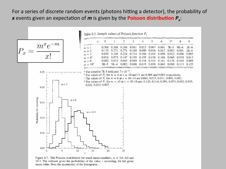
For a series of discrete random events (photons hiEng a detector), the probability of x events given an expecta$on of m is given by the Poisson distribu,on Px:
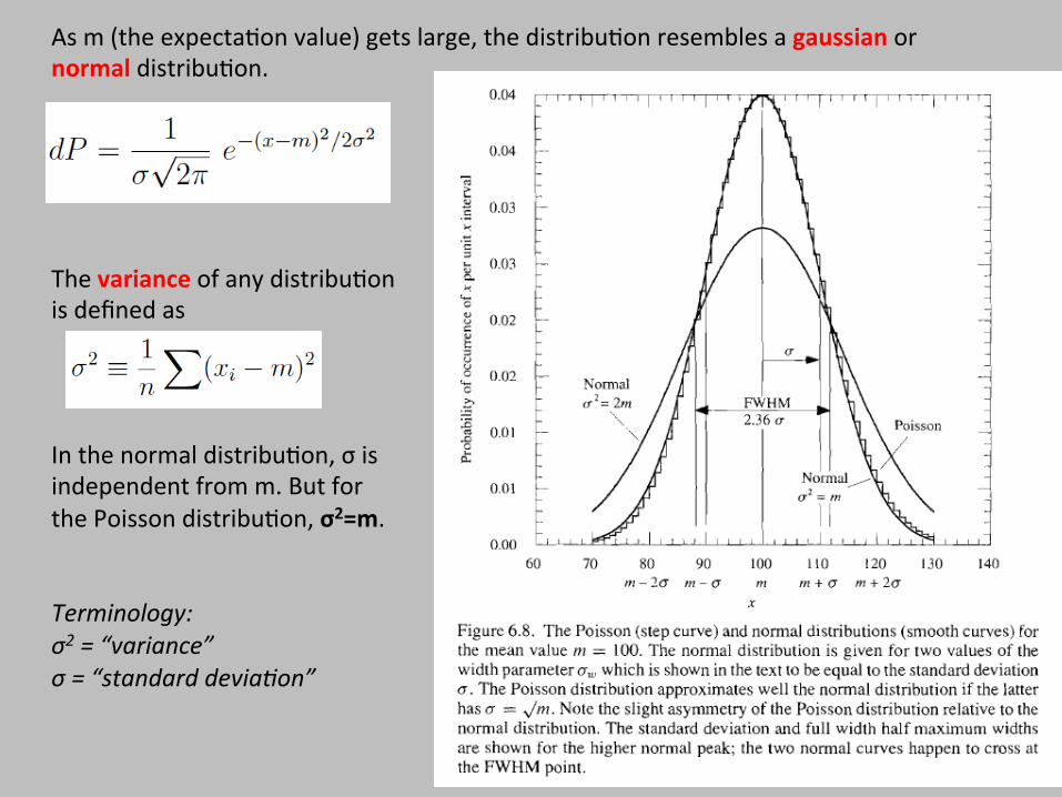
As m (the expecta$on value) gets large, the distribu$on resembles a gaussian or normal distribu$on.
The variance of any distribu$on is defined as
In the normal distribu$on, σ is independent from m. But for the Poisson distribu$on, σ2=m. Terminology: σ2 = “variance” σ = “standard deviaNon”
Detec,on significance Say the background sky gives m=100 photons per pixel. By Poisson stats, the uncertainty in the sky level is then σ=√m =√100 = 10 photons. So the sky level is 100 ± 10 photons. How faint of a (one pixel) star could you detect? N* = 10 photons è 1σ detec$on, very likely to be just a sky fluctua$on. A poor detec$on. N* = 30 photons è 3σ detec$on, likelihood of a sky fluctua$on is small. A good detec$on!
A more rigorous signal-‐to-‐noise calcula$on Consider measuring the flux from a star in an aperture that includes npix pixels. Signal: • N*, the total number of photons from the star. Noise: • Total Poisson noise from the star: σ = √N* • Per-‐pixel Poisson noise from the sky: σ = √NS • Per-‐pixel Poisson noise from dark current: σ = √ND • Per-‐pixel CCD read noise σ = NR
These noise contribu$ons add in quadrature, so we get
“The CCD Equa$on” see Howell, Chapter 4.4
These N’s all refer to photons or electrons, not counts!
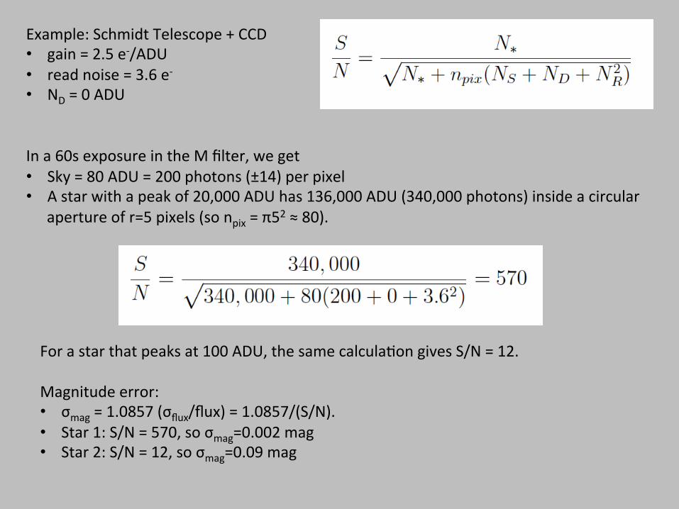
In a 60s exposure in the M filter, we get • Sky = 80 ADU = 200 photons (±14) per pixel • A star with a peak of 20,000 ADU has 136,000 ADU (340,000 photons) inside a circular
aperture of r=5 pixels (so npix = π52 ≈ 80).
For a star that peaks at 100 ADU, the same calcula$on gives S/N = 12. Magnitude error: • σmag = 1.0857 (σflux/flux) = 1.0857/(S/N). • Star 1: S/N = 570, so σmag=0.002 mag • Star 2: S/N = 12, so σmag=0.09 mag
S/N scaling with exposure ,me
Case 1: Bright objects N* dominates, so S/N ≈ N*/√N* ≈ √N* Since N* scales with exposure $me, S/N ~ √texp Case 2: Detector limited NR dominates, so S/N ≈ N*/NR NR is independent of exposure $me, so S/N ~ texp
Random vs Systema,c Error Precision: How well can you measure a quan$ty? How repeatable is your measurement? Usually captured by “random errors.” Accuracy: How well does your measurement actually recover the value you are trying to measure? Source of “systema$c errors.” Precision vs Accuracy / Random vs Systema$c is cri$cal to understand, extremely hard to quan$fy in prac$ce. If you measure a value and do not give some esNmate of uncertainty or some discussion of systemaNc errors, your measurement is useless.
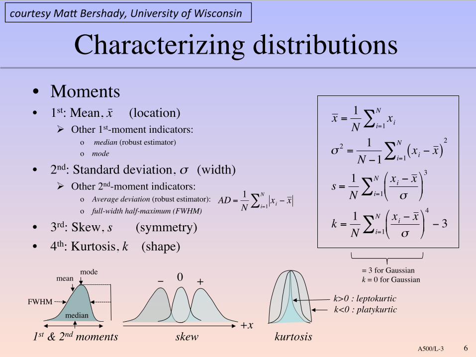
Characterizing distributions!• Moments!• 1st: Mean, x (location)!
! Other 1st-moment indicators:!o median (robust estimator)!o mode!
• 2nd: Standard deviation, σ (width)"! Other 2nd-moment indicators: !
o Average deviation (robust estimator):!o full-width half-maximum (FWHM)!
• 3rd: Skew, s (symmetry)!• 4th: Kurtosis, k (shape)!
A500/L-3!
€
x = 1N
xii=1
N∑
σ 2 =1
N −1xi − x ( )
i=1
N∑
2
s =1N
xi − x σ
%
& '
(
) *
i=1
N∑
3
k =1N
xi − x σ
%
& '
(
) *
i=1
N∑
4
− 3
€
AD =1N
xi − x i=1
N∑
+x!skew!
0! +!�"k>0 : leptokurtic!k<0 : platykurtic!
kurtosis!
= 3 for Gaussian!k = 0 for Gaussian!
mode!mean!
median!
1st & 2nd moments!
FWHM!
6!
courtesy MaV Bershady, University of Wisconsin
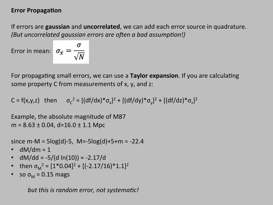
Error Propaga,on If errors are gaussian and uncorrelated, we can add each error source in quadrature. (But uncorrelated gaussian errors are oZen a bad assumpNon!) Error in mean: For propaga$ng small errors, we can use a Taylor expansion. If you are calcula$ng some property C from measurements of x, y, and z: C = f(x,y,z) then σC2 = [(df/dx)*σx]2 + [(df/dy)*σy]2 + [(df/dz)*σz]2 Example, the absolute magnitude of M87 m = 8.63 ± 0.04, d=16.0 ± 1.1 Mpc since m-‐M = 5log(d)-‐5, M=-‐5log(d)+5+m = -‐22.4 • dM/dm = 1 • dM/dd = -‐5/(d ln(10)) ≈ -‐2.17/d • then σM2 = [1*0.04]2 + [(-‐2.17/16)*1.1]2 • so σM = 0.15 mags
but this is random error, not systemaNc!
Correla,ons Linear: • y = mx +b • mul$dimensional: z = mx + ny + b Nonlinear: try to linearize them!
Example #1: Exponen$al surface brightness of a disk
Raw form: I(r)=I0e-‐r/h Linearized form: ln(I) = ln(I0) – r/h In surface brightness:
remember log(x)=ln(x)/log(10)
Example #2: Power law form form of Tully-‐Fisher
Raw form: L ~ Vcircα
Linearized form: log(L) = αlog(Vcirc) + C
Correla,ons Pearson’s correla$on coefficient, r, measures linear correla$on between two variables.
Slope(s), intercept, and their uncertain$es: m ± σm, b ± σb RMS scawer around the fit:
But, beware……..
Anscombe’s quartet: Fit y=mx+b and get the same r, m, b, σm, σb, σRMS
Modeling Uncertainty Let’s say you have used your data to es$mate some parameter. For example, you have a set of x,y data points and you’ve fit a line to the data and es$mated a slope and intercept. How do we es$mate our uncertain$es on these values: Least squares fiIng: what usually comes out of your computer. Implicitly assumes uncorrelated Gaussian sta$s$cs. Different algorithms can give different es$mates, par$cularly in low-‐N or presence of outliers. Resampling (non-‐parametric): • Jack-‐knife: go through your data i=1,N $mes, tossing out data point i and redoing you
es$mate. Look at varia$on. • Bootstrap: go through your dataset picking out N data points at random. Do this as
many $mes as you can stand, look at varia$on.
Bayesian Es,ma,on We speak in terms of probabili$es. What is the probability you’d get the data you measure given some underlying model? Bayes’ theorem: A = your dataset B = the parameter you’re trying to measure P(B|A): The posterior probability. What is the probability of B, given that you’ve measured A? Your best es$mate is the B that is most-‐likely. P(A|B): The likelihood func:on. What is the probability of measuring A, given that model B is true? P(B): The prior. What is the probability of B? P(A): Normalizing factor. What is the probability you could measure A to begin with?
Bayesian Es,ma,on Let’s get specific, but simple. The luminosity func$on of a galaxy cluster – the number of galaxies as a func$on of their luminosity, N(L). Adopt the Schecter func$on: N(L) ~ Lαe-‐L/L* You’ve measured a bunch of galaxy luminosi$es – how do you es$mate α and L*? Classical: bin in L, plot N(L), do a chi-‐sq fit, solve for α and L* Bayesian:
• A = your measurements • B = the LF parameters α and L* • P(A|B) = probability of measuring my dataset given some par$cular value of α
and L*, in other words the model for the luminosity func$on. • P(B) = my prior beliefs about α and L* • P(B|A) = the probability that I’d get my data given some par$cular (α, L*) pair