State Estimation, Observability and B d DBad Data

EE 521 Analysis of Power Systems

Chen-Ching Liu, Boeing Distinguished ProfessorWashington State University

Concept of State Estimation (Wood, Wollenberg)

21

100 MW

2

60 MW

M12 (meter)

65 MW40 MWM13

M32

Use the measurements M13 = 5 MW = 0.05 p.u. and M32 = 40 MW = 0.40 p.u.

35 MW (TRUE VALUE)5 MW3

1

p.u.40.01

p.u.05.01

23

3113

x

x

ff f

10.0 ,002.0 findcan we,0213

23

x

Two measurements are sufficient. This example assumes meters are perfectly accurate.

If all 3 meters have some errors. For example,M12 = 62 MWM13 = 6 MWM32 = 37 MW

If only M13 & M32 are used, use DC load flow to show 2 92 25 MW 2 1 M12 58.25 MW

TRUE Values in parentheses)

92.25 MW

(100)

M13

M32

37 MW (40)(MATCHED)

p )64.25 MW

(65)

6 MW(5)

MATCHED

0331 MW

(35)

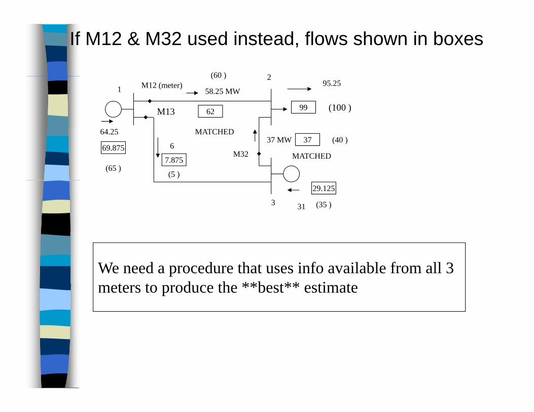
If M12 & M32 used instead, flows shown in boxes

2(60 )

1

(100 )

2

58.25 MW

M13

M12 (meter)

9962

95.25(60 )

64.2537 MW

M32

37 (40 )MATCHED

MATCHED69.875

(65 )

6

7.875

(5 )

313 (35 )

29.125

We need a procedure that uses info available from all 3 t t d th **b t** ti tmeters to produce the **best** estimate

Maximum Likelihood+

Xtrue

l r1-volts

Want to estimate the value of the 111

zz truemeas

Want to estimate the value of the voltage source xtrue

Note { mean value of Z meas}=Z true if Note { mean value of Z1meas}=Z1

true if 1has zero mean

Normal Distribution with Zero Mean

Probability density function (PDF) is normal

zz truemeas11 (random error)

Probability density function (PDF) is normal

-exp1 )( 2

2

PDF

i

deviation standard

2p

2)(

21

2

11

PDF( )variance1 PDF()

Small 1 better measurement quality

10

So the PDF of Z1meas

2

1

2

1 211exp

21 )(

)( zz truemeasPDF

If r1

is know, then

2

)( xmeas

2

11 21

1exp

21 )(

)(r

zmeas

PDF

Want to find an estimate that maximizes the probability density that the observed measurement Z1

meas would occur

Therefore, we can

2

meas1

1

)PDF( log max z

xz meas

x

2

1

1

21

1

2log-max r

zx

2

11

rx

z meas

or

2

121max r

x

2

11

min rx

z meas

or

2

12min

x

Find xest by

rx

z meas2

011

x 2

1

02

zrx measest

or

11

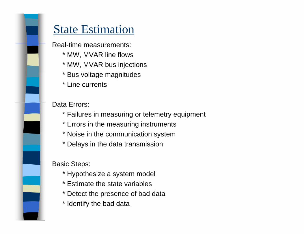
State EstimationR l ti tReal-time measurements:

* MW, MVAR line flows* MW, MVAR bus injections* B lt it d* Bus voltage magnitudes* Line currents

D t EData Errors:* Failures in measuring or telemetry equipment* Errors in the measuring instruments* N i i th i ti t* Noise in the communication system* Delays in the data transmission

B i SBasic Steps:* Hypothesize a system model* Estimate the state variables* Detect the presence of bad data* Identify the bad data

Benefits of State Estimation:

Can reduce # of transducers and remote terminal units.

Bad data detection and identification.

State Estimation: Problem Formulation

STATIC STATE ESTIMATOR

Measurements z

Structure SEstimated system state &

model

(Computer Algorithms)Parameter Values p

Notation: t: continuous, tn: discrete (n=1,2,…)Unknown independent variables:

• Node injection Complex, nonstationary, environmentally dependentvector-valued stochastic process

ty~

• True structure Binary type stochastic process

t~

• True parameter values Line, transformer, meter data

t~

Unknown State Variables: Node VoltagesThe power flow equation now reads

K titi

tttt xfy

~~~_~

,,

Known quantities: Measurements

line flows bus injections voltage magnitudes

tn_

line flows, bus injections, voltage magnitudes Pseudo measurements

nontelemetered information on line flows, injections,, j ,voltages.

Parameter values ntp_

note that: Parameter value error

S

nznn tvttp~

__

ntzv

_ S Structure ntS

_

nnn ttt CS___

(error)

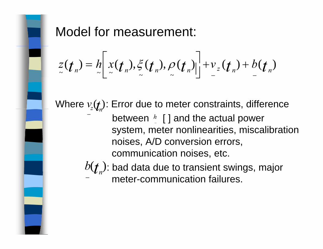
Model for measurement:

)()()(),(),()(__~~~~~ tttttt nnznnnnbvxhz

Where : Error due to meter constraints, difference

)(tnzvbetween [ ] and the actual power system, meter nonlinearities, miscalibration noises A/D conversion errors

)(_ tnz

_h

noises, A/D conversion errors, communication noises, etc.

: bad data due to transient swings, major )(tnb g , jmeter-communication failures.

)(_ tn

Static State Estimator:1 Hypothesize model: determine1. Hypothesize model: determine

))(),(,()(____ tt nnxhxh

p

s

__

__

and the measurement error covariance matrix__

)()( tt TER

2. State estimate value of which minimizes the

)()(__tvtv nznzER

:)(^

tx n xresidual _ _

))(()()(___txhtzt nnn

3. Detection: Test to decide if bad data or structural error exist

___

4. Identification:Test to decide which measurements or structural data are incorrect

Four Basic Operations of Static State EstimationSCADA

Measurement z_ParameterStructure s

_

p_

Hypothesize modelassume vbc p,,

______000

obtain Rxh ),(__

E i i Fi d ( i i i )^ Modify

Estimation: Find (minimize )x_

_

Detection: Check assumptionsb i if i

Y

yinput

, by testing if is small enoughEND No

_00

____, bc

Identification: Logic to determine location of bad data & structural error

Estimation:Weighted least Square (WLS)Algorithm

M t M d lMeasurement Model(sym)

)(

z

_~__~

RE Tz

z

vv

bvxhz

Suppose no bad data b=0, then~

z~

vv

zvxhz~~

)(

To minimize the residual We minimize

__

)(__~~xhz

)]([)]([)(___

1

____xhzxhzx RJ T

Why: Assume that the n components of are jointlyGaussian, then the joint probability density function is given by

y~

function is given by

)()(1exp1)( 11/22/ yyRyyf mmy T

)()(

2p

R)(det)2()(

__

__

1/22/_~

yyyyyf mmy n

where R is the covariance matrix and is the mean ofym

~

y~

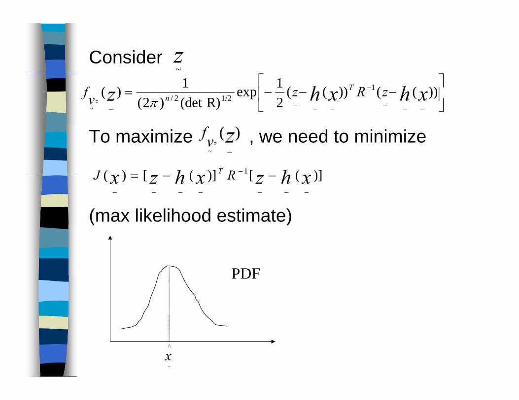
Consider

z~

))(())((

21exp

R) (det)2(1)(

___

1

___1/22/_~

xhxhz zRzvfT

nz

To maximize , we need to minimize)(_~zzvf

)]([)]([)( 1 xhxhx RJ T

(max likelihood estimate)

)]([)]([)(_______xhzxhzx RJ

( )

PDFPDF

x^

_

0))((2)(

_

_1

____

_

hxh

xhzxx

RJ

T

0))((

H where0))((2

___

1

_

_1

___

xhzxh

xhz

RH

HR

T

T

Necessary condition for optimality

(1)0)()(2)(

1_

xhzxx

RHJ

T

T

Where is the Jacobian

(1) 0)()(2____

_

xhzxx

RH

xh_H

To solve (1), the following iterative algorithm is usedx_

___

1

__1_(3) )]([)(][ xhzRxHxxG ii

Tiii

Note that if i= 1 converges to then_

^

_1_, xxx ii

x^xNote that if , i= 1,…,converges to thenix_ _x

)2( 0)]([___

1 xhzRH T

Question: How to choose Gi (Gain matrix)^^

Suppose , then (3&4) yields

seriesTaylor (4)))(()()(________ iii xxxHxhxh

)()(^xHxH i ____

))(()(_

^

___

1

__ iiiT xxxHRxH

C ith (3)

))(()(___

1

__ iiT xhzRxH

Compare with (3)

)()( 1ii

T

ixRx HHG

(Information matrix)

__

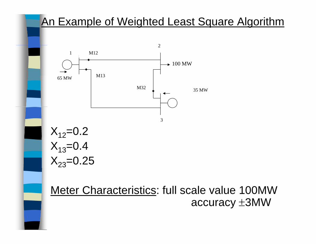
An Example of Weighted Least Square Algorithm

21

100 MW

2

M13

M12

35 MW

65 MW M13

M32

X12=0.23

12X13=0.4X23=0.25

Meter Characteristics: full scale value 100MW 3MWaccuracy 3MW

Interpretation: Normal distribution density N(0,1)

Prob{ 3 3} = 0 99

Mean-3-3MW

3+3MW

Prob{-3 3} = 0.99

The meter will give a reading within interval forg g 99% of the time.

= 1MW = 0.01 (p.u.)

DC Load Flow

11313

211212

BzBz

BBB

1121212

23232

0

-

z

Bz

BB

232

13

32

13

5- 5

- 0

0

zz

2

1

MatrixCovariance4- 0 0 2.5

1010

4-

4-

2

13

2

12

0 0

0 0

0 0

0 0

R

Matrix Covariance

10 10

4-2

32

13

0 0 0 0

WLS Estimatef (1)0))((1 hRHT from eq(1)0))((

___

1 xhzRHT

111^

0zx RHHRH TT

4

41

4

4

__

0.060.62

0 0

0 0

4-05-0 2.5 5

0 2.55- 5

0 0

0 0

4-05-0 2.5 5

1010

1010

^

1

44

028571.0

0.37 0 04- 0 5-

4- 0 0 04- 0 5-

10 10

R id l

^

2

094286.0

Residual

][][),(^

1^

21 xHzxHz RJ T

2.14 ______

Reading:Reading:

Power Generation, Operation & ControlJohn Wiley & Sons A WoodJohn Wiley & Sons, A. Wood, B. Wollenberg, 1996, Chapter 12.

Network Observability (Wu and Monticelli)

DC load flowLine flows )(

__

θθ

θBp

Bf

Line flows

Let Y=diag{Bij}, then the vector of line flow

)( jiijijθθBf

measurements can be written as

The true line flows are given by

__θHz

T θYAf The true line flows are given by

Where Y=diag{Bij}

__θYAf

j

H, A include the datum node (unreduced)

A network is said to be observable if any flow in the network can be observed by some sort of i di i i h findication in the set of measurements.

In other words, whenever there is any nonzeroIn other words, whenever there is any nonzero flow in the network, at least one of the measurements should be nonzero.

Definition: A network is said to be observableif for all such that the line flows

_

00 fz

0__ Hz

___

____

0 TYAf

Any state for whichIs called an unobservable state .

_

*

_

T

_

*

_0A ,0 H*

_

For an unobservable state *Let then branch (i, j) is an unobservable branch.

_0 ,A *

ij*

_

T*

_ if

unobservable branch.

Q:How to check the observability of the t k?network?

We will show that

The network is observable if and only if has a full rank, where is obtained from H by deleting any column.

_

H_

H

Why: (A:unreduced)____10 AT

where any real number and = [1,1,…1]T

(1) If th t k i b bl th

_1

(1) If the network is observable, then

_____00 TAHz

So we obtain(i (th l i ))

10____

H

(i.e., (the column sum is zero)) __01 H

Define H= To show has a full rank _H

_h

_H

___

Now suppose

00____

H

0_

_

_

_H

Let then

_

_

_ 0

0

0_

__0

or

H

Hence is of full rank.

0__

or

_H

(2) On the other hand, if is of full rank, and, then

H_

0___

HZ

_

k

k

k

hH

hHhH

__

_

_

_

_

__

_

0

Now k

TT

hHHH_

_1

___

_

__

Nowthe column sum of H is always equal to zero (why) 1 ( y)

hence 0

1

1

_

_

hH

or

1

1

__

_1

__

__

_

hHHH

hHTT

ityobservabil

therefore,

01___

_

_

__

AT

k

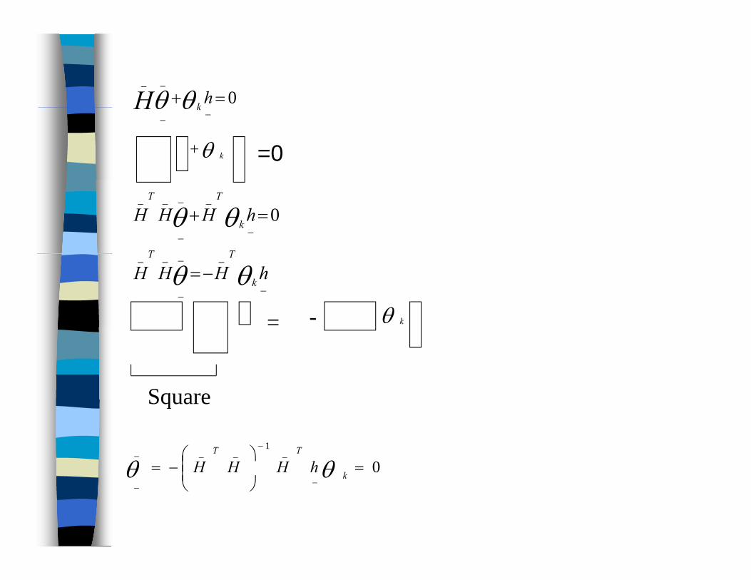
0__

hkH __kH

=0 k

_

__

_

__0hHHH

TT

k

TT

_

__

_

__hHHH k

TT

= - k

SquareSquare

0_

1___

k

TT

hHHH__

k

ExampleLi 1 21

Line 4Li 2

Line 1 2

Line 2

iLine 34 3

10011001 114

zz

011001101001

4

3

2

32

23

41z

zzz

Node Incidence Matrix

011000111001

32

A

11000110

Delete one column of H

00

00

11

_

H

1

11

100H

Rank = 2H_

is not of full rank H_

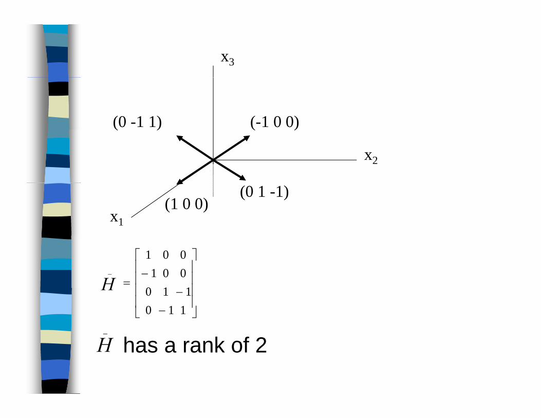
x3

(-1 0 0)(0 -1 1)

x2

( )( )

x1(1 0 0)

(0 1 -1)

1

00

100

01

1_

H

has a rank of 2

1

11

100H

H_

has a rank of 2H

*

_

*

*

TA

*

3*

2*

1*

34

23

12

10011100

01100011

*

*

*

Now suppose (zero measurements)

4*

14

1001*

_

* 0HThen , and Line flows

_0*

4*

1 0*

3*

2

0*

*

3*

2*

23

2*

1*

12

Unobservable branches

0*

*

4*

1*

14

4*

3*

34

Unobservable state: 1= 4 , 2 = 3

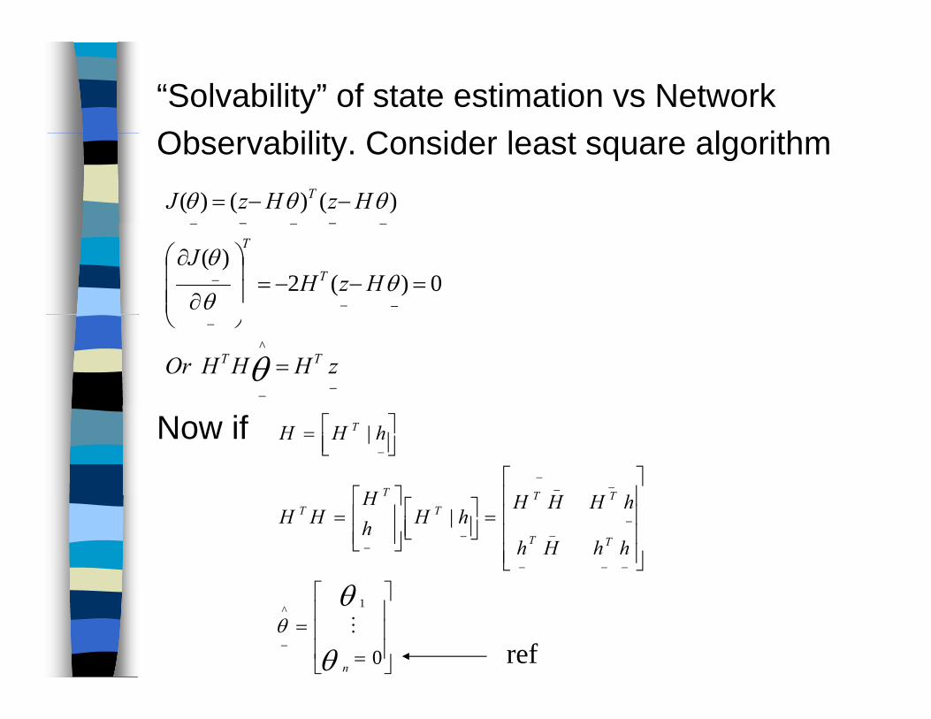
“Solvability” of state estimation vs Network Ob bilit C id l t l ithObservability. Consider least square algorithm

)()()( HzHzJ T

__

_

_____

0)(2)(

HzHJ

T

T

__

^

_

zHHHOr TT

Now if

|

__

_

_

TTT

T

hHHHH

hHH

|

__

_

_

__

_

TT

TTT

TT

hhHh

hHHHhHh

HHH

0

1^

_

n

ref

0

1 _

_

_

___

hhh

hHHHH

TT

TT

T H

1

0

_

_

__

___

_

zHHH

hhHh

T

TT

TT

1

1

_

_

_

__

_

__

_

_

zHHH

zhHhTT

TT

Now suppose the network is observable, then is of full rank, therefore exists, and

_

H1

__

HH

T

zHHHT

_

_1

__

_1

is solved uniquely. (Solvability)* Pseudo measurements are often used for

estimation of unobservable states.

Identification of Bad DataWeighted Least Square

T

___

1

___

__

T

xhzRxhz

rr

J

T

The WLS estimate satisfies

2

1

m

i i

ir

x

The WLS estimate satisfies

2

_

___

1

xxhzRH

xxddJ T

x_

J bithih

2 __

1 0__

hH

rRHd

xx

T

now

Jacobiantheis where

____

_

_

_

vxhz

xH d

1

00

_

b

dIth meter is bad

___bvv z

0

d: size of bad data

Define the state estimation errorxxx

Suppose is small, andx

___

x_

xhxh H

1

_____

& ,Then 0

T xhvxhRH

xhxh xH

1

,______,

0

0

T hh

xhvxhRH

11

______

1

_0

T

T xhvHxhRH x

Also, for ,covariance matrix 11where

x

T HRHzvv

_

_

(why?) E__

x

T

Xx

Now for the residual vectorzzr___

xhvxh____

xhvHxh x_____

vvRHxH T

_

1

_

_

vRHxHI T 1

_

_

Where the residual sensitivity matrixvr W

__

T 1

RH TxHIW 1

For , the residual covariancezvv__

rE rrT

WRxHR

rE

H

rrT

(why?)

__

Now define the diagonal matrix rdiagD

*Weighted residualg

1

* Normalized residual

rRrw

_

1

_

Normalized residual

rDrN

_

1

_

Then for , covarianceszvv__

rr UwwET

W__

AndRR r 11

rr UNE N

T

DD r

N

11

__

Note that diagonal elements of UN are all equal to 1to 1.

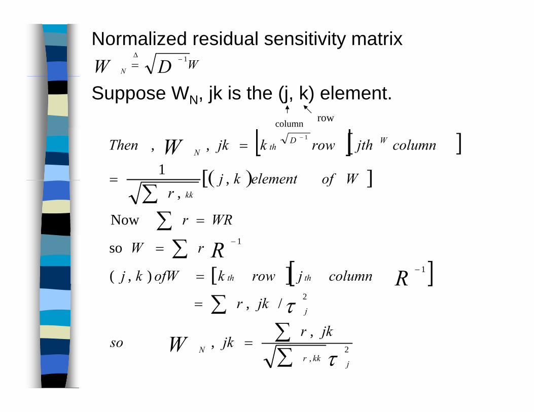
Normalized residual sensitivity matrix1WDW N

Suppose WN, jk is the (j, k) element.

column row

1

, ,1 WD

thN

Wofelementkj

columnjthrowkjkThen W

Now

,, kk

WRr

Wofelementkjr

1

1

),(

so

thth columnjrowkofWkj

rW

RR

2

,

/, j

jkr

jkrR

2,

,,

jkkr

N

jkjkso W

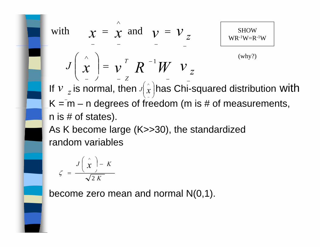
zvvxx___

and with

SHOWWR-1W=R-1W

zJ vWRvx T

Z

1

_

(why?)

If is normal, then has Chi-squared distribution with K = m – n degrees of freedom (m is # of measurements,

Z ____ zv

_

xJ_

g ( ,n is # of states).As K become large (K>>30), the standardized

d i blrandom variables

KJ x

become zero mean and normal N(0,1).

K2

Bad data detection

HypothesesH : no bad data or structural errorsH0 : no bad data or structural errorsH1 : H0 is not true

Let Pe : prob. of rejecting H0 when H0 is actually tr e (“False alarm”)true (“False alarm”)

Pd : prob. of accepting H1 when H1 is true(d t ti )(detection)

t t

1. - test

xJ_

Accept H0 if Reject H0 (accept H1) otherwise

1

1Reject H0 (accept H1), otherwise when is normal, K is large and H0

i t th i N(0 1) S 1 65zv

_

1

is true, then is N(0,1). So = 1.65 corresponds to Pe = 0.005

1

2. RN – testA t H if

Accept H0 if Reject H0 otherwise

mkkNr ,...,1, ,

3 R – test3. Rw testAccept H0 isR j t H th i

mkkwr ,...,2,1, ,

Reject H0 otherwise

For single or multiple non-interacting Bad data

Ordered residual search:weighted (normalized) residuals

Nrrweighted (normalized) residuals

put into a descending order of magnitude.The measurement z corresponding to the

Nw rr__

The measurement zi corresponding to the largest residual rw

max (rnmax) is removed first,

etcetc.Grouped residual search:

the p largest residuals in or removedr Nrthe p largest residuals in or removed simultaneously and then put back one after another until bad data is detected.

wr_

Nr_

References[1] “Bad Data Analysis for Power System State Estimation,” E. Handschin et al.IEEE Trans. Power Apparatus and Systems, Mar/April 1975, pp. 329-337.[2] A M ti lli “El t i P S t St t[2] A, Monticelli, “Electric Power System State Estimation,” Proceedings of the IEEE, Feb. 2000, pp. 262-282.