Daedalus Dakota (18m/s stall) State-space models for the unsteady lift force due to agile maneuvers and gusts Steve Brunton & Clancy Rowley Princeton University FAA/JUP January 20, 2011 Monday, March 21, 2011
Transcript
Daedalus Dakota (18m/s stall)
State-space models for the unsteady lift force due to agile maneuvers and gusts
Steve Brunton & Clancy RowleyPrinceton University
FAA/JUP January 20, 2011Monday, March 21, 2011
FLYIT Simulators, Inc.
Motivation
Predator (General Atomics)
Applications of Unsteady Models
Conventional UAVs (performance/robustness)
Flow control, flight dynamic control
Autopilots / Flight simulators
Gust disturbance mitigation
Need for State-Space Models
Need models suitable for control
Combining with flight models
Wake Vortex Shadow (Aerocam)Monday, March 21, 2011
2.7.2.2 Unmanned Aircraft SystemsUAS operations are some of the most demanding operations in NextGen. UAS operations include scheduled and on-demand flights for a variety of civil, military, and state missions.
Because of the range of operational uses, UAS operators may require access to all NextGen airspace. ...
5.3.3 Weather Information Enterprise Services•! Enterprise Service 3: UASs Are Used for Weather Reconnaissance. [R-169]En route weather reconnaissance UASs are equipped to collect and report in-flight weather data. Specialized weather reconnaissance UASs are used to scout potential flight routes and trajectories to identify available “weather-favorable” airspace...
2.7.2.3 Vertical Flight... Rotorcraft are also used for UAS applications for commercial, police, and security operations. These operations add to the density and complexity of operations, particularly in and around urban areas.
3.3.1.2.3 Integrated Environmental OperationsUAS performing security functions and the airport perimeter security intrusion detection system may have the capability to assist with wildlife management programs.
NextGen ConOps V2.0: UAVs
Monday, March 21, 2011
AC 00-54 Appendix 1
U/25/88
2.3.3 ENCOUNTER ON APPROACH
Analysis of a typical windshear en- counter on approach provided evidence of an increasing downdraft and tailwind
along the approach flight path (Figure 20). The airplane lost airspeed, dropped below the target glidepath, and contacted the ground short of the runway threshold.
Figure 20. Windshear encounter during approach. (1) Approach initially appeared normal. (2) Increasing downdraft and tailwind encountered at transition. (3) Airspeed decrease combified with reduced visual cues resulted in pitch attitude reduction. (4) Airplane crashed short of approach end of runway.
Page 22
11125188 AC 00-54 Appendix 1
2.3.1 ENCOUNTER DURING TAKEOFF - AFTER off the runway (Figure 13). For the LIFTOFF first 5 seconds after liftoff the
takeoff appeared normal, but the air- In a typical accident studied, the plane crashed off the end of the run- airplane encountered an increasing way about 20 seconds after liftoff. tailwind shear shortly after lifting
3
~ 2
1 4
Runway
Figure 13. Windshear encounter during takeoff after liftoff. (1) Takeoff initially appeared normal. (2) Windshear encountered just after liftoff. (3) Airspeed decrease resulted in pitch attitude reduction. (4) Aircraft crashed off departure end of runway 20 set after liftoff.
Page 15
AC 00-54 Appendix 1
11125188
o The Microburst as a Windshear Threat
Identification of concentrated, more powerful downdrafts--known as micro- bursts--has resulted from the inves- tigation of windshear accidents and from meteorological research. Micro- bursts can occur anywhere convective weather conditions (thunderstorms, rain showers, virga) occur. Observa- tions suggest that approximately five percent of all thunderstorms produce a microburst.
Downdrafts associated with microbursts are typically only a few hundred to 3,000 feet across. When the downdraft reaches the ground, it spreads out horizontally and may form one or more horizontal vortex rings around the downdraft (Figure 7). The outflow region is typically 6,000 to 12,000 feet across. The horizontal vortices may extend to over 2,000 feet AGL.
Cloud Base
0
Downdraft
1 Scale 1OOOft
I Xl\\ I I
Figure 7. Symmetric microburst An airplane transiting the microburst would experience equal headwinds and tailwinds.
Page 8
11/25/88 AC 00-54 Appendix 1
Microburst outflows are not always symmetric (Figure 8). Therefore, a significant airspeed increase may not occur upon entering the outflow, or
may be much less than the subsequent airspeed loss experienced when exiting the microburst.
Cloud Base \ toooft
Approx
L- Scale
0 lOOOft
Wind
-Downdraft
Horizontal Vortex-
Outflow Front1 -outflow- Figure 8. Asymmetric microburst. An airplane transiting the microburst from left to
right would experience a small headwind followed by a large failwiqd.
Page 9
Microburst Windshear
Navigating a microburst requires counterintuitive piloting
M.L. Psiaki and R.F. Stengel, J. Aircraft: vol. 23, no. 8, 1986.
S.S. Mulgund and R.F. Stengel, J. Guidance: vol. 16, no. 6, 1993.
D.A. Stratton and R.F. Stengel, J. Guidance: vol. 15, no. 5, 1992.
Monday, March 21, 2011
Stall velocity and size
RQ-1 Predator (27 m/s stall)
Daedalus Dakota (18m/s stall)
Puma AE(10 m/s stall)
Smaller, lower stall velocity
Vstall =�
2ρ
(CLmaxS)−1 W
S
W
L
CL
V
Wing surface area
Aircraft weight
Lift force
Lift coefficient
Velocity of aircraft
Monday, March 21, 2011
UAV Flight Envelope
1. Landing approach speed is 30% higher than stall speed
Vstall =�
2ρ
(CLmaxS)−1 W
2. occurs at the stall speed CLmax Vstall
CLmax ∈ [1, 1.5]
for reasonable aspect ratio
W = Lmax = CLmax qS
= CLmax ·�
12ρV 2
stall
�· S
i.e.
S
W
L
CL
V
Wing surface area
Aircraft weight
Lift force
Lift coefficient
Velocity of aircraft
Monday, March 21, 2011
3 Types of Unsteadiness
1. High angle-of-attack
α > αstall
Large amplitude, slow Moderate amplitude, fast
2. Strouhal number
St =Af
U∞
3. Reduced frequency
k =πfc
U∞
Small amplitude, very fast
� �� �Closely related
αeff = tan−1 (πSt)
Brunton and Rowley, AIAA ASM 2009
Monday, March 21, 2011
3 Types of Unsteadiness
3. Reduced frequency
k =πfc
U∞
Small amplitude, very fast
1. High angle-of-attack
α > αstall
Large amplitude, slow Moderate amplitude, fast
2. Strouhal number
St =Af
U∞
� �� �Closely related
αeff = tan−1 (πSt)
Brunton and Rowley, AIAA ASM 2009
(flutter instability, fast gust disturbance, rapid maneuver)
Monday, March 21, 2011
D V
!
"
Iyy q = M
mV ! = L + T sin(") ! mg sin(!)mV = T cos(") ! D ! mg sin(!)
" = q ! (L + T sin(") ! mg cos(!)) /mV
x = Ax + Bu
y = Cx + Du
!"#$%&'()*+,#-.
/0123)*+,#-.
TL
M
q
coupled model
Coupled Flight Dynamic Model
Interesting control scenario when time-scales of flight dynamics are close to time-scales of aerodynamics
Monday, March 21, 2011
Candidate Lift Models
CL = CL(α)
CL = CLαα
CL = 2πα
Motivation for State-Space Models
Computationally tractable
fits into control framework
Captures input output dynamics accurately
CL(t) = CδL(t)α(0) +
� t
0Cδ
L(t− τ)α(τ)dτ Wagner’s Indicial Response
Theodorsen’s Model
CL =π
2
�h+ α− a
2α�
� �� �Added-Mass
+2π
�α+ h+
1
2α
�1
2− a
��
� �� �Circulatory
C(k)
Leishman, 2006.
Theodorsen, 1935.
Wagner, 1925.
Monday, March 21, 2011
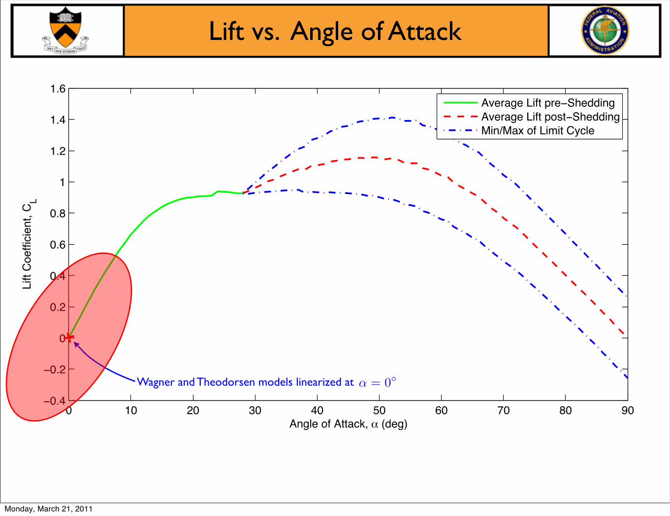
Lift vs. Angle of Attack
0 10 20 30 40 50 60 70 80 900.4
0.2
0
0.2
0.4
0.6
0.8
1
1.2
1.4
1.6
Angle of Attack, (deg)
Lift
Coe
ffici
ent,
C L
Average Lift pre SheddingAverage Lift post SheddingMin/Max of Limit Cycle
Low Reynolds number, (Re=100)
Hopf bifurcation at αcrit ≈ 28◦ (pair of imaginary eigenvalues pass into right half plane)
Monday, March 21, 2011
Lift vs. Angle of Attack
0 10 20 30 40 50 60 70 80 900.4
0.2
0
0.2
0.4
0.6
0.8
1
1.2
1.4
1.6
Angle of Attack, (deg)
Lift
Coe
ffici
ent,
C L
Average Lift pre SheddingAverage Lift post SheddingMin/Max of Limit Cycle
Need model that captures lift due to moving airfoil!
Monday, March 21, 2011
Lift vs. Angle of Attack
0 10 20 30 40 50 60 70 80 900.4
0.2
0
0.2
0.4
0.6
0.8
1
1.2
1.4
1.6
Angle of Attack, (deg)
Lift
Coe
ffici
ent,
C L
Average Lift pre SheddingAverage Lift post SheddingMin/Max of Limit CycleSinusoidal (f=.1,A=3)
Need model that captures lift due to moving airfoil!
Monday, March 21, 2011
Lift vs. Angle of Attack
0 10 20 30 40 50 60 70 80 900.4
0.2
0
0.2
0.4
0.6
0.8
1
1.2
1.4
1.6
Angle of Attack, (deg)
Lift
Coe
ffici
ent,
C L
Average Lift pre SheddingAverage Lift post SheddingMin/Max of Limit CycleSinusoidal (f=.1,A=3)Canonical (a=11,A=10)
Need model that captures lift due to moving airfoil!
Monday, March 21, 2011
0 10 20 30 40 50 60 70 80 900.4
0.2
0
0.2
0.4
0.6
0.8
1
1.2
1.4
1.6
Angle of Attack, (deg)
Lift
Coe
ffici
ent,
C L
Average Lift pre SheddingAverage Lift post SheddingMin/Max of Limit CycleSinusoidal (f=.1,A=3)Canonical (a=11,A=10)
Lift vs. Angle of Attack
! " # $ % & ' ("&
#!
#&
)*+,-./0.)11234
! " # $ % & ' (
!5&
"
"5&
#
67
89:-
.
.;<=>?).@A$B. A!>?).@A$B. A"&
Need model that captures lift due to moving airfoil!
Monday, March 21, 2011
Lift vs. Angle of Attack
0 10 20 30 40 50 60 70 80 900.4
0.2
0
0.2
0.4
0.6
0.8
1
1.2
1.4
1.6
Angle of Attack, (deg)
Lift
Coe
ffici
ent,
C L
Average Lift pre SheddingAverage Lift post SheddingMin/Max of Limit Cycle
Wagner and Theodorsen models linearized at α = 0◦
Monday, March 21, 2011
Theodorsen’s Model
Apparent Mass
Not trivial to compute, but essentially solved
force needed to move air as plate accelerates
Increasingly important for lighter aircraft
Circulatory Lift
Need improved models here
source of all lift in steady flight
Captures separation effects
k =πfc
U∞
2D Incompressible, inviscid model
Unsteady potential flow (w/ Kutta condition)
Linearized about zero angle of attack
Leishman, 2006.
Theodorsen, 1935.
CL =π
2
�h+ α− a
2α�
� �� �Added-Mass
+2π
�α+ h+
1
2α
�1
2− a
��
� �� �Circulatory
C(k)
C(k) =H
(2)1 (k)
H(2)1 (k) + iH
(2)0 (k)
Monday, March 21, 2011
Empirical Theodorsen
CL =π
2
�h + α− a
2α�
� �� �Added-Mass
+ 2π
�α + h +
12α
�12− a
��
� �� �Circulatory
C(k)
CL = C1
�α− a
2α�
+ C2
�α +
12α
�12− a
��C(k)
L [CL]L [α]
= C1
�1s −
a2
�+ C2
�1s2 + 1
2s
�12 − a
��C(s)
Generalized Coefficients
Transfer Function
Added MassCL+
Quasi-SteadyCL(!e!)
C(s)!
C2
!1s2
+12s
"12! a
#$
C1
"1s! a
2
#
Monday, March 21, 2011
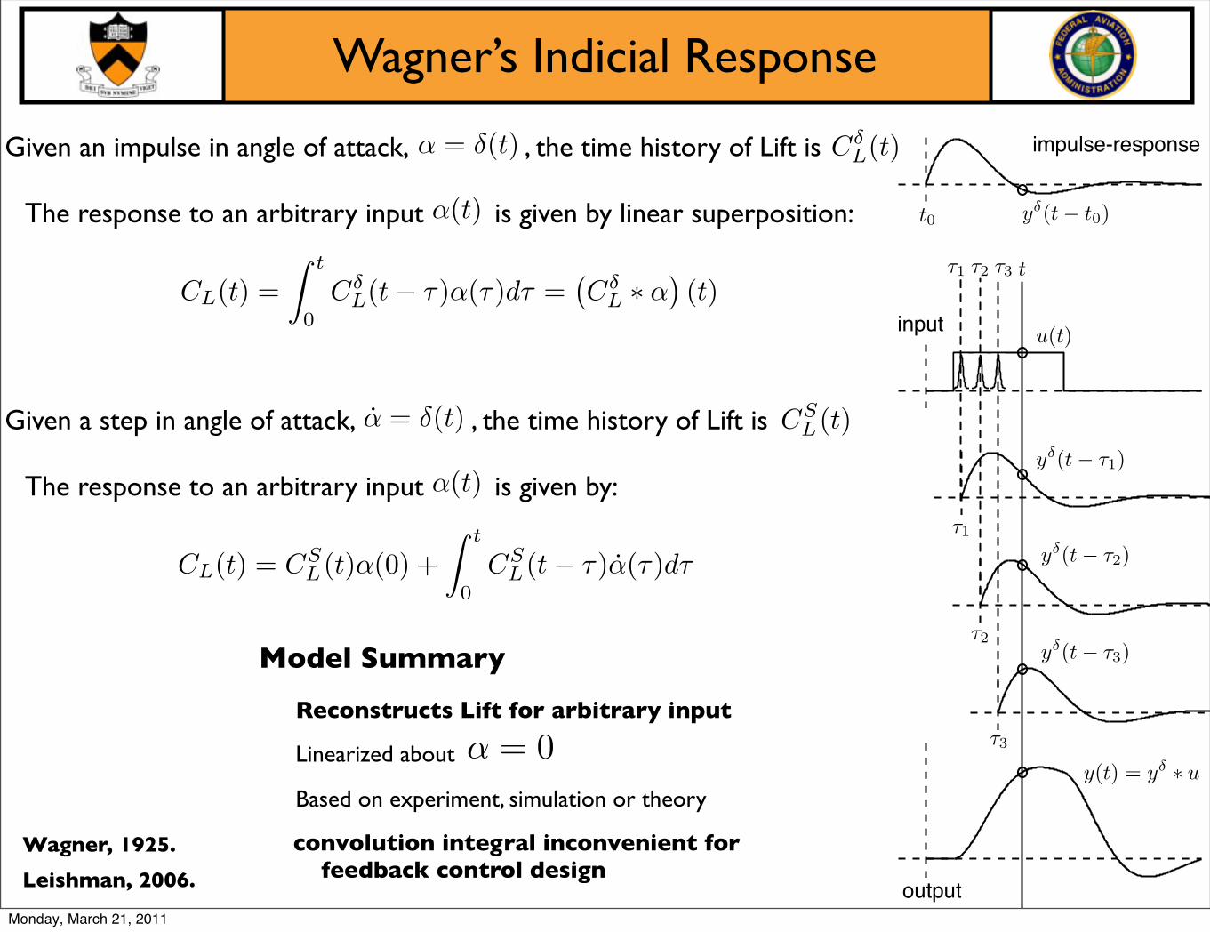
Wagner’s Indicial Response
Model Summary
convolution integral inconvenient for feedback control design
Reconstructs Lift for arbitrary input
Linearized about
Based on experiment, simulation or theory
α = 0
Leishman, 2006.
Wagner, 1925.
u(t)
!1 !2 !3 t
!"#$%
&$%#$%
!1
!2
!3
!'#$()*+,*)#&")*
t0
y!(t ! !1)
y!(t ! !2)
y!(t ! !3)
y(t) = y! " u
y!(t ! t0)
CL(t) = CSL(t)α(0) +
� t
0CS
L(t− τ)α(τ)dτ
CL(t) =
� t
0Cδ
L(t− τ)α(τ)dτ =�Cδ
L ∗ α�(t)
Given an impulse in angle of attack, , the time history of Lift is
The response to an arbitrary input is given by linear superposition:α(t)
CδL(t)α = δ(t)
Given a step in angle of attack, , the time history of Lift is
The response to an arbitrary input is given by:
CSL(t)α = δ(t)
α(t)
Monday, March 21, 2011
Reduced Order Wagner
CL(α, α, α,x) = CLαα+ CLα α+ CLα α+ Cx
Y (s) =
�CLα
s2+
CLα
s+ CLα +G(s)
�s2U(s)
d
dt
xαα
=
Ar 0 00 0 10 0 0
xαα
+
Br
01
α
CL =�Cr CLα CLα
�
xαα
+ CLα α
Stability derivatives plus fast dynamics
Transfer Function
State-Space Form
Quasi-steady and added-mass Fastdynamics
Monday, March 21, 2011
Reduced Order Wagner
+ CL
G(s)
!"#$%&$'(#)*+,+#))()+-#$$
.#$'+)*/#-%0$
CL!
CL!
s
CL!
s2
!
Brunton and Rowley, in preparation.
Model Summary
ODE model ideal for control design
Based on experiment, simulation or theory
Linearized about α = 0
Recovers stability derivatives associated with quasi-steady and added-mass
CLα , CLα , CLα
quasi-steady and added-mass
ERA Model
input
fast dynamics
d
dt
xαα
=
Ar 0 00 0 10 0 0
xαα
+
Br
01
α
CL =�Cr CLα CLα
�
xαα
+ CLα α
CL(t) = CSL(t)α(0) +
� t
0CS
L(t− τ)α(τ)dτ
Monday, March 21, 2011
Bode Plot - Pitch (LE)
Frequency response
Model without additional fast dynamics [QS+AM (r=0)] is inaccurate in crossover region
Models with fast dynamics of ERA model order >3 are converged
output is lift coefficient CL
Punchline: additional fast dynamics (ERA model) are essential
input is ( is angle of attack)α α
Brunton and Rowley, in preparation.
10 2 10 1 100 101 10240
20
0
20
40
60
Mag
nitu
de (d
B)
10 2 10 1 100 101 102180
160
140
120
100
80
60
40
20
0
Phas
e (d
eg)
Frequency (rad U/c)
QS+AM (r=0)ERA r=2ERA r=3ERA r=4ERA r=7ERA r=9
Pitching at leading edge
Monday, March 21, 2011
Bode Plot - Pitch (QC)
Frequency response
Reduced order model with ERA r=3 accurately reproduces Wagner
Wagner and ROM agree better with DNS than Theodorsen’s model.
output is lift coefficient CL
input is ( is angle of attack)α α
Brunton and Rowley, in preparation.
Pitching at quarter chord
Asymptotes are correct for Wagner because it is based on experiment
Model for pitch/plunge dynamics [ERA, r=3 (MIMO)] works as well, for the same order model
Canonical pitch-up, hold, pitch-down maneuver, followed by step-up in vertical position
Reduced order model for Wagner’s indicial responseaccurately captures lift coefficient history from DNS
OL, Altman, Eldredge, Garmann, and Lian, 2010
Monday, March 21, 2011
Lift vs. Angle of Attack
0 10 20 30 40 50 60 70 80 900.4
0.2
0
0.2
0.4
0.6
0.8
1
1.2
1.4
1.6
Angle of Attack, (deg)
Lift
Coe
ffici
ent,
C L
Average Lift pre SheddingAverage Lift post SheddingMin/Max of Limit Cycle
Wagner and Theodorsen models linearized at α = 0◦
Monday, March 21, 2011
Lift vs. Angle of Attack
0 10 20 30 40 50 60 70 80 900.4
0.2
0
0.2
0.4
0.6
0.8
1
1.2
1.4
1.6
Angle of Attack, (deg)
Lift
Coe
ffici
ent,
C L
Average Lift pre SheddingAverage Lift post SheddingMin/Max of Limit Cycle
Wagner and Theodorsen models linearized at α = 0◦
Monday, March 21, 2011
Bode Plot of ERA Models
10 2 10 1 100 101 10250
0
50
100Frequency Response for Leading Edge Pitching
Mag
nitu
de (d
B)
10 2 10 1 100 101 102200
150
100
50
0
Phas
e
Frequency
=0=5=10=15=20=25
Results
At larger angle of attack, phase converges to -180 at much lower frequencies. I.e., solutions take longer to reach equilibrium in time domain.
Lift slope decreases for increasing angle of attack, so magnitude of low frequency motions decreases for increasing angle of attack.
Consistent with fact that for large angle of attack, system is closer to Hopf instability, and a pair of eigenvalues are moving closer to imaginary axis.
Monday, March 21, 2011
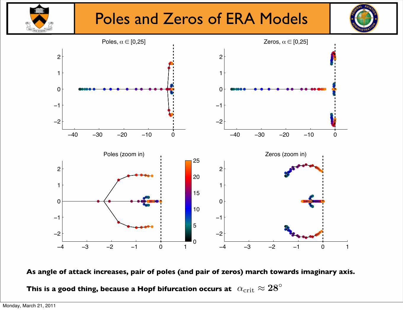
Poles and Zeros of ERA Models
4 3 2 1 0 1
2
1
0
1
2
Poles (zoom in)
4 3 2 1 0 1
2
1
0
1
2
Zeros (zoom in)
40 30 20 10 0
2
1
0
1
2
Poles, [0,25]
40 30 20 10 0
2
1
0
1
2
Zeros, [0,25]
0
5
10
15
20
25
As angle of attack increases, pair of poles (and pair of zeros) march towards imaginary axis.
This is a good thing, because a Hopf bifurcation occurs at αcrit ≈ 28◦
Monday, March 21, 2011
Poles and Zeros of ERA Models
4 3 2 1 0 1
2
1
0
1
2
Poles (zoom in)
4 3 2 1 0 1
2
1
0
1
2
Zeros (zoom in)
40 30 20 10 0
2
1
0
1
2
Poles, [0,25]
40 30 20 10 0
2
1
0
1
2
Zeros, [0,25]
0
5
10
15
20
25
As angle of attack increases, pair of poles (and pair of zeros) march towards imaginary axis.
This is a good thing, because a Hopf bifurcation occurs at αcrit ≈ 28◦
Reduced order model based on indicial response at non-zero angle of attack
- Based on eigensystem realization algorithm (ERA)- Models appear to capture dynamics near stall- Locally linearized models outperform models linearized at α = 0◦
Empirically determined Theodorsen model
- Theodorsen’s C(k) may be approximated, or determined via experiments- Models are cast into state-space representation- Pitching about various points along chord is analyzed
Brunton and Rowley, AIAA ASM 2009-2011
OL, Altman, Eldredge, Garmann, and Lian, 2010
Leishman, 2006.
Wagner, 1925.
Theodorsen, 1935.
Breuker, Abdalla, Milanese, and Marzocca, AIAA 2008.
Future Work:
- Combine models linearized at different angles of attack - Add large amplitude effects such as gust disturbance or wake vortex