1 STATES AND MARKETS: THE ADVANTAGE OF AN EARLY START Valerie Bockstette Areendam Chanda Louis Putterman * Abstract: In this paper, an index of the depth of experience with state-level institutions, or state antiquity, is derived for a large set of countries. We show that state antiquity is significantly correlated with measures of political stability and institutional quality, with income per capita, and with the rate of economic growth between 1960 and 1995. State antiquity contributes significantly to the explanation of differences in growth rates even when other measures of institutional quality, conventional explanatory variables, and region dummies are controlled for. It is also a good instrument for “social infrastructure,” which explains cross-country differences in worker productivity. Keywords: Economic Growth, Economic Development, Comparative Economic Systems, JEL Classifications: O40, O10, P50 Introduction States and markets have sometimes been viewed as competitors, but in the last decade, there has been increasing agreement that a capable state can play an important * No affiliation; Department of Economics, North Carolina State University; Department of Economics, Brown University. Send comments to [email protected]. We thank the World Bank for its support of part of this project and related research. We are grateful to Atsushi Inoue for his assistance with part of the estimating work.
Transcript
1
STATES AND MARKETS: THE ADVANTAGE OF AN EARLY START
Valerie Bockstette
Areendam Chanda
Louis Putterman*
Abstract: In this paper, an index of the depth of experience with state-level institutions, or
state antiquity, is derived for a large set of countries. We show that state antiquity is
significantly correlated with measures of political stability and institutional quality, with
income per capita, and with the rate of economic growth between 1960 and 1995. State
antiquity contributes significantly to the explanation of differences in growth rates even
when other measures of institutional quality, conventional explanatory variables, and
region dummies are controlled for. It is also a good instrument for “social
infrastructure,” which explains cross-country differences in worker productivity.
States and markets have sometimes been viewed as competitors, but in the last
decade, there has been increasing agreement that a capable state can play an important
* No affiliation; Department of Economics, North Carolina State University; Department of Economics, Brown University. Send comments to [email protected]. We thank the World Bank for its support of part of this project and related research. We are grateful to Atsushi Inoue for his assistance with part of the estimating work.
2
facilitating role in the process of economic development.1 A number of studies have
explored the empirical connection between measures of political stability and
bureaucratic competence, on the one hand, and rates of economic growth, on the other.2
There is some evidence from these, and also arguments at the case study level, that a
stable and competent state is indeed a contributing factor in economic growth. But what
gives rise to effective states?
In this paper, we investigate the possibility that differences not only in state
capacity but more broadly, in the capacity to mount an effective drive toward economic
development, derive in part from very long run historical processes giving rise to
different potentials for growth. We develop an index of the antiquity of the state, and
show that it is a robust predictor of recent economic growth in the presence of a variety
of economic, institutional, and regional controls. We show that the index is correlated
with indicators of current institutional capacity and stability, but has predictive power in
growth equations even when the latter are controlled for. We show that while the
antiquity of the state appears to predict the level of development in some simple
regressions, this predictive power declines as one moves towards earlier post-War years
and it vanishes in the presence of additional controls. Finally, we show that while the
antiquity of the state is not a robust proximate determinant of the level of development, it
is an effective instrument for the social infrastructure variable used in Hall and Jones
(1999).
Early States and Modern Growth
3
Imagine a series of political maps of the world, in which the areas occupied by
kingdoms, empires, or states are shaded, the rest unshaded. By 10,000 BC, there is
human habitation in all of the continents except Antarctica, but the map of the world
remains entirely unshaded, since people live in small bands or clan groups and there are
no signs of political structures uniting even a few thousand individuals. By 1500 BC, the
map would be shaded in portions of Mesopotamia and of the Nile, Indus, and Yellow
River valleys and would remain unshaded almost everywhere else. On the eve of
Columbus’s 1492 voyage, the map would be more widely shaded, but would remain
unshaded for large parts of the Americas and Africa, all of Australia, and smaller portions
of Europe and Asia. By 2000 AD, the inhabited world would be fully shaded and
comprised of nation states. A review of the earlier maps would make it clear that some
of today’s nations (for example, China) have histories stretching back thousands of years,
while others (for example, New Guinea) have much shorter state histories.
A longer history of statehood might prove favorable to economic development
under the circumstances of recent decades for several reasons. There may be learning by
doing in the ways of public administration, in which case long-standing states, with larger
pools of experienced personnel, may do what they do better than do newly formed states.
The operation of a state may support the development of attitudes consistent with
bureaucratic discipline and hierarchical control, making for greater state (and perhaps
more broadly, organizational) effectiveness. An experienced state like China seems to
have been capable of fostering basic industrialization and the upgrading of its human
capital stock even under institutions of government planning and state property in the
1960s and 1970s, whereas an inexperienced state like Mozambique sewed economic
disaster when attempting to pursue similar policies a few years later. Such differences
4
may carry over to a market setting -- contrast, for instance, the late 20th Century
economic development of Japan and South Korea, modern countries with ancient national
histories, with that of the Philippines, a nation that lacked a state before its 16th Century
colonization by Spain.
Historically, the technological, social and economic development of the world’s
societies between Neolithic times and the present was not a one step process of leaping
from a “backward” or “traditional” economy to a “modern” and industrial one. Instead,
there were multiple steps involving a transition from hunting and gathering in small
bands to the development of settled village agricultures to the rise of more densely settled
agrarian states with currencies and taxation and finally the development of modern
enterprise systems, markets, and public sectors (Boserup, 1965, Diamond, 1998). While
the shifts to village agriculture and then to agrarian states predated the rise of modern
industry by a thousand years or longer in places like southern Europe and China, some
societies have tried to collapse the transition to an industrial society from one of village
agriculture, pastoralism, or hunting and gathering, into a generation or two. There are
indications that this is difficult, perhaps in part due to limits on the rate of change of
social attitudes and capabilities. Statistical evidence suggests that position on the
densely populated agrarian state end of the continuum of pre-modern societies has been
conducive to economic growth in the latter part of the 20th Century (Burkett, Humblet
and Putterman, 1999, Chanda and Putterman, 2000). While those studies use Boserupian
indicators like population density to measure the stage of development, the presence of an
early state may be an equally good indicator of early development, or may reflect
dimensions of early development that the other indicators miss.
5
Finally, as Diamond argues with reference to China, nationhood fosters linguistic
unity. With nationhood and a common language may come a sense of common identity.
These factors may be helpful for the avoidance of the civil wars and other forms of
political instability that have had devastating impacts on many economies (Easterly and
Levine, 1997). A unified state and a common language and identity may also facilitate
the trust and ease of social interaction discussed in the literature on social capital
(Putnam, 1993, Knack and Keefer, 1997; Temple, 1998).
Related Literature
The idea that differences in state effectiveness or in other forms of “social
capability” underlie differences in levels and rates of economic growth has been
suggested by a number of contributors to the recent literature on economic growth.
Abramowitz (1986) argues that a “country’s potential for rapid growth is strong not when
it is backward without qualification, but rather when it is technologically backward but
socially advanced.” Temple and Johnson (1998) find that after controlling for initial
income per capita, the average economic growth rates for the period 1960-85 for sixty
countries for which the required data are available are higher for countries with higher
values of a modernization or “social development” index based on measures in Adelman
and Morris (1967). The index continues to be a significant predictor of economic growth
after controlling also for human capital and investment rates, suggesting that social
capability works through channels not captured by the investment rates, formal schooling
measures or the initial level of development.
6
Hall and Jones (1999) postulate that differences in capital accumulation, total
factor productivity and output per worker are driven by differences in “social
infrastructure,” which they define as “institutions and government policies that determine
the economic environment within which economic individuals accumulate skills, [and]
firms accumulate capital and produce output.” The authors proxy “social infrastructure”
by the mean of (a) an index of country risk to international investors, and (b) an index of
openness to international trade. To account for the likely two-way relationship between
income levels and social infrastructure, they attempt to identify exogenous instruments
for that variable. They find that distance from the equator, the extent to which French,
German, Spanish, and especially English are spoken as first languages and the predicted
trade share of an economy, are effective predictors of social infrastructure. Using these
variables as instruments, they find that variations in social infrastructure can account for a
25.2-fold difference (out of an overall 35.2-fold difference) in output per worker across
economies.
Another “social” variable that has received much recent attention in economics as
well as in sociology and political science is “social capital”. Used extensively by
sociologists such as James Coleman (1988), the term was introduced into economics by
Loury (1977), who used it to describe the “authority regulations, relations of trust and
consensual allocation of rights which establish norms.”3 This usage overlaps with but
differs slightly from that of sociologists, for instance Narayan (1997), who uses social
capital to refer to “the quantity and quality of associational life and related norms” (p. 1)
and to “the rules, norms, obligations, reciprocity, and trust embedded in social relations,
social structures, and society’s institutional arrangements which enable its members to
achieve their individual and community objectives” (p. 50). In recent discussions of
7
social capital in economics, the concept is related to the extent of trust, associational
memberships, and general social and political participation (Temple, 1998). Robert
Putnam’s (1993) argument that a more vibrant associational life leads to better
government and economic performance was based on observations in northern Italy and
has been accorded great attention by economists.
Knack and Keefer (1997) try to measure the importance of social capital to
economic growth by constructing indicators of the level of “trust” and “civic norms” for
twenty-nine market economies, based on the World Values Survey. They find that both
indicators are significant predictors of per capita income growth in the period 1980-1992.
Furthermore, both measures are higher in countries that effectively protect property rights
and contracts and in countries that are less polarized along lines of ethnicity and class.
Countries with higher amounts of both also have lower economic inequality (as measured
by the Gini coefficient). Unfortunately, the sample of countries for which the required
measures are available consists mainly of developed and middle-income economies.
La Porta, Lopez-de-Silanes, Shleifer and Vishny (1998) examine the laws
governing investor protection, the enforcement of these laws, and the extent of
concentration of ownership of shares in firms across countries. On a similar historical
note they find that countries with different legal histories offer different types of legal
protection to their investors. Most countries’ legal rules, either through colonialism,
conquest or outright borrowing, can be traced to one of four distinct European legal
systems: English common-law, French civil-law, German civil-law and Scandinavian
civil-law. They show that countries whose legal rules originate in the common law
tradition offer the greatest protection to investors. As far as law enforcement is
concerned, German civil-law and Scandinavian civil-law countries emerge superior. The
8
French civil-law countries offer both the weakest legal protection and the worst
enforcement. These legal origin variables have been increasingly adopted as exogenous
determinants of institutional quality in the economic growth literature. In particular,
given their usefulness in predicting various indicators of investor rights and protection,
they have been used widely as instrumental variables for financial market development.4
A last set of studies that are worthy of remark in view of their relationship to the
present one are those of Acemoglu, Johnson and Robinson (2001, 2002), who study the
histories of countries colonized by Europeans after 1500. They argue that where
European settlement was discouraged by settler susceptibility to disease (Acemoglu et
al., 2001) or where the extraction of surpluses was favored by the presence of dense,
urbanized, and relatively prosperous populations (Acemoglu et al., 2002), institutions
suited to extraction rather than investment were put in place, leading to an eventual
“reversal of fortunes” wherein the low-density countries (often settled by large numbers
of Europeans) overtook the high-density (usually indigenous majority) countries in level
of development. While Acemoglu et al.’s “reversal” may help to explain why we do not
find early states to be proximate determinants of contemporary development levels, those
authors do not consider the advantage that early states may have conferred in the
“catching up” phase of 1960-1995.
State History: Construction and Correlations
Do countries having a longer history of state-level institutions perform better on
indicators of political stability and bureaucratic quality? In levels of income and rates of
economic growth? To explore these questions, one first needs a measure of the antiquity
9
of the state. Finding no existing series of data ready to hand, we compiled a rough index
of state antiquity as follows.5 We began by dividing the period from 1 to 1950 C.E. into
39 half centuries.6 For each period of fifty years, we asked three questions (and allocated
points) as follows: 1. Is there a government above the tribal level? (1 point if yes, 0 points
if no)7; 2. Is this government foreign or locally based? (1 point if locally based, 0.5 points
if foreign [i.e., the country is a colony], 0.75 if in between [a local government with
substantial foreign oversight]8; 3. How much of the territory of the modern country was
ruled by this government? (1 point if over 50%, 0.75 points if between 25% and 50%, 0.5
points if between 10% and 25%, 0.3 points if less than 10%).9 Answers were extracted
from the historical accounts on each of 119 countries in the Encyclopedia Britannica.
The scores on the three questions were multiplied by one another and by 50, so that for a
given fifty year period, what is today a country has a score of 50 if it was an autonomous
nation, 0 if it had no government above the tribal level, 25 if the entire territory was ruled
by another country, and so on. We then combined the data for the 39 periods,
experimenting with different ways of “discounting” to reduce the weight of periods in the
more remote past.10 Finally in order to make the series easier to interpret, the resulting
sum was divided by the maximum possible value the series could take given the same
rate of discounting the past. Thus the value that the index can take for any given country
lies between zero and one.
Most of our correlation and regression results are robust over a range of
assumptions about how rapidly the effect of the past is dissipated; to simplify exposition,
we focus on a series we will call statehist5, which reduces the weight on each additional
half century by a moderate 5%.11 Table 1 shows the average values of statehist5 for seven
macro regions, with region averages calculated using country populations in 1960 as
10
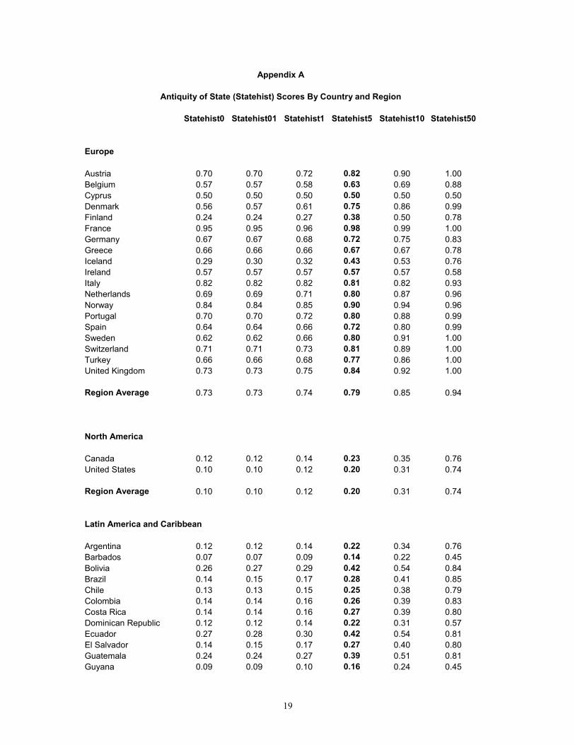
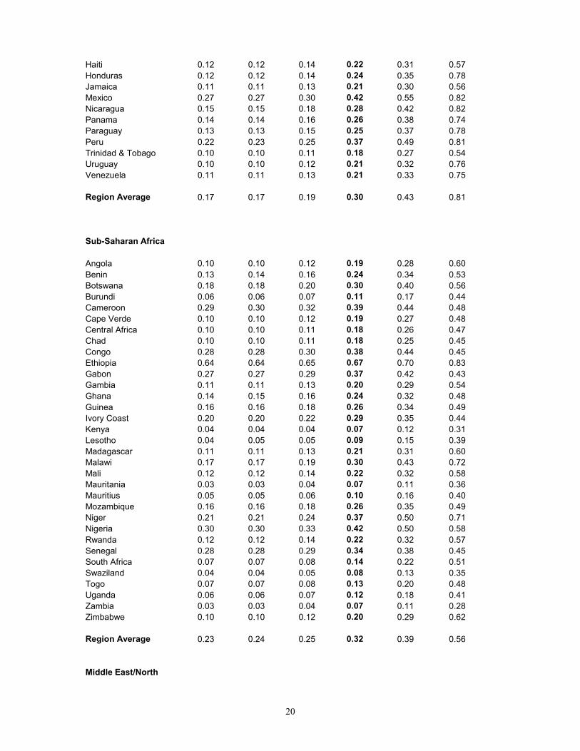
weights. Appendix A shows individual country values of statehist5 and versions of the
index for alternative rates of discounting the past. The highest value of statehist5 is 1, for
China, while the lowest value is 0.066, for Zambia. Appendix B lists the correlations of
statehist5 with variants of the measure which place different weights on the past.
Appendix C shows how the index is formed by reviewing two country examples: Italy
(statehist5 = 0.81), and Mexico (statehist5 = 0.42).
In Table 2, we present simple correlations between statehist5 and sets of political
and institutional quality indicators, social and demographic indicators, and measures of
per capita income and growth, calculated (with one exception) for the maximal sample of
countries for which relevant data are available. These correlations provide strong support
for the conjecture that a long state history is conducive both to better contemporary state
performance and to a higher income and growth.
The International Country Risk Guide (ICRG) published by Political Risk
Services—a firm that specializes in assessment of risk in various countries—provides
data on various indicators of the quality of governance. These include measures of a)
corruption b) government repudiation of contracts, c) expropriative risk d) rule of law,
and e) bureaucratic quality, among others.12 As is apparent, Statehist5 is significantly
positively correlated with all of these variables. It is also positively correlated with
Mauro’s (1995) index of political stability. Countries with high values of statehist5 also
experienced fewer political assassinations during 1965-69.13 However, political
instability was lower in these countries if measured by the number of riots and of
government crises.14
11
Table 2 also shows statehist5 to be significantly positively correlated with the
level of real GDP per capita for various years (1960, 1970, 1980, 1990 and 1995) and
with the average rate of growth of real GDP per capita between 1960 and 1995.15 An
interesting feature of Table 2 is that statehist5 is found to be more correlated with per
capita income as time unfolds, and more strongly correlated still with the growth rate of
income. One reason why this might be the case is that the positive effect of statehist5
becomes increasingly visible as the negative impact of colonialism fades away.
Equivalently, less developed countries with longer histories of national-level experience
displayed a greater relative advantage in income generation after two or three decades of
policy experimentation than at the outset of the post-colonial era.16
The types of correlations seen here do not, of course, imply causality. Although
the long run nature of statehist5 means we needn’t worry about reverse causality, it is
possible that the state variables are proxying for more direct determinants of political
system performance, income levels, and growth. Statehist5 may proxy for geographic
region, which could influence the growth rate for reasons that remain unclear to us. Early
states are associated with higher population densities, and Table 2 shows this correlation
to persist when looking at population density in 1960. Could the latter be the real cause
of faster growth? Another example, mentioned above, is that an early national
government is likely to be associated with greater linguistic homogeneity, which several
studies suggest is associated with more rapid growth. Table 2 shows that statehist5 is
indeed negatively correlated with the main index of ethno-linguistic heterogeneity
(ETHNIC) used by Easterly and Levine, significant at the .01 level. State experience
may also be correlated with modernization or social development, as studied by Temple
and Johnson (1998). Their social development index, covering mainly developing
12
countries, is significantly positively correlated with statehist5 when the sample excludes
Latin America, but there is no correlation in this case for the full sample.17 Also
statehist5 has a strong correlation with Knack and Keefer’s (1997) measure of civic
norms, although it is less strongly correlated with their measure of trust. Finally, we have
seen that statehist5 is correlated with various measures of contemporary state quality.
Might these be treated as the proximate causes of faster growth, with the age of the state
per se being of no further interest in its own right?18
Relationship with Recent Economic Growth: Multivariate Analysis
The relationship between the rate of recent economic growth and the length of
state experience is the main focus of our paper. The correlation between the two
variables that is reported in Table 2 is shown graphically in Figure 1, which plots the
values of statehist5 against the growth rate of GDP per capita in 1960-95 for the 94
countries for which the two series are available. To check whether an early state is
associated with the rate of growth after other influences are controlled for, Table 3
reports a set of exercises in which statehist5 and related variables are added to a set of
cross-country growth regressions modeled on those of Barro (1991) and Mankiw, Romer
and Weil (MRW, 1992). Column 1 shows a baseline regression including only the core
explanatory variables studied by MRW.19 The dependent variable is the growth rate of
real GDP per capita from 1960 to 1995, and the independent variables are logarithm of
per capita GDP in 1960, the secondary school enrollment rate of 1960 (Schooling), the
population growth rate for 1960 to 1995 20, and the logarithm of the average gross
domestic investment share of GDP from 1960 to 1995.21 In Column 2, we add statehist5
13
and find that it has a positive coefficient significant at the 1% level. The addition of
statehist5 increases the proportion of the variance explained by the regression from about
47% to almost 58%.
Figure 2 presents a scatter plot of the orthogonalized residuals for growth rate and
statehist5 after controlling for all the above variables. A visual inspection of the scatter
plot confirms the positive association between the two variables. However, it also clearly
shows Hong Kong (HKG) to be an important outlier.22 To ensure that our results are not
driven by Hong Kong, the regression in column (2) was repeated in column (3) after
dropping Hong Kong.23 The significance of statehist5 is retained. How important is
statehist5 quantitatively? To get a sense of how much having a longer experience with
governments could raise growth rates, consider the following exercise: suppose that
Mauritania, the country which recorded the second lowest value for statehist5 (0.068),
instead had the statehist5 value of China, the highest in the sample (1.0). Based on the
estimated coefficient in column (3), this would mean Mauritania would have recorded an
annual increase of 1.9% in its growth rate. Given that Mauritania’s average growth rate
during the 35-year period was nearly zero and China’s was 3.8%, differences in statehist5
can, by these calculations, explain half the difference in growth rates between the two
countries.
As we have seen, the recent literature on economic growth has recognized the
importance of quality of institutions. There is no doubt that the arguments being made for
the importance of a well-developed state has a bearing on issues of institutional quality.
Therefore, it is important to check that statehist5 does not simply proxy the former. To
control for this, Column 4 adds an institutional quality variable (ICRG) which is the
average of the five ICRG variables discussed earlier. The coefficient on the ICRG
14
measure is significant and has the expected positive sign. Adding the ICRG variable
actually tends to increase the significance of statehist5 though it comes at the cost of
reduced sample size.
Burkett et al. (op. cit.) conjecture that the level of pre-modern development,
conceptualized as lying on a continuum from the hunting-and-gathering band to the large-
scale agrarian state, may have facilitated economic growth in recent decades, helping to
explain why, for instance, growth was higher in China and South Korea than in Zaire and
New Guinea. They estimate growth regressions like those of Table 3 in which they add,
to a specification resembling column, three alternative proxies for level of pre-modern
development, including population density (see Boserup, op cit.). The results strongly
support their conjecture. Is the significance of statehist5 in Table 3’s regressions
attributable to a distinctive effect of an early state, or is it simply substituting for other
measures of early development, e.g. population density, in these equations? In column 5
of Table 3 we add 1960 population density, which is available for all but one country in
our sample, to the regression of column 3. The result shows that both an early state and a
dense population are associated with more rapid modern economic growth; the two
variables each have significant positive coefficients in this regression.
We have discussed above the relationship between an early state and ethnic
homogeneity. A regression adding the ethnic heterogeneity measure ETHNIC is shown
in column 6. We find that statehist5 retains its explanatory power, while the coefficient
on ETHNIC is negative but not significant. Finally, Column 7 embeds all the earlier
specifications and also adds region dummies which cover the entire world.24 Statehist5
continues to be robust.
15
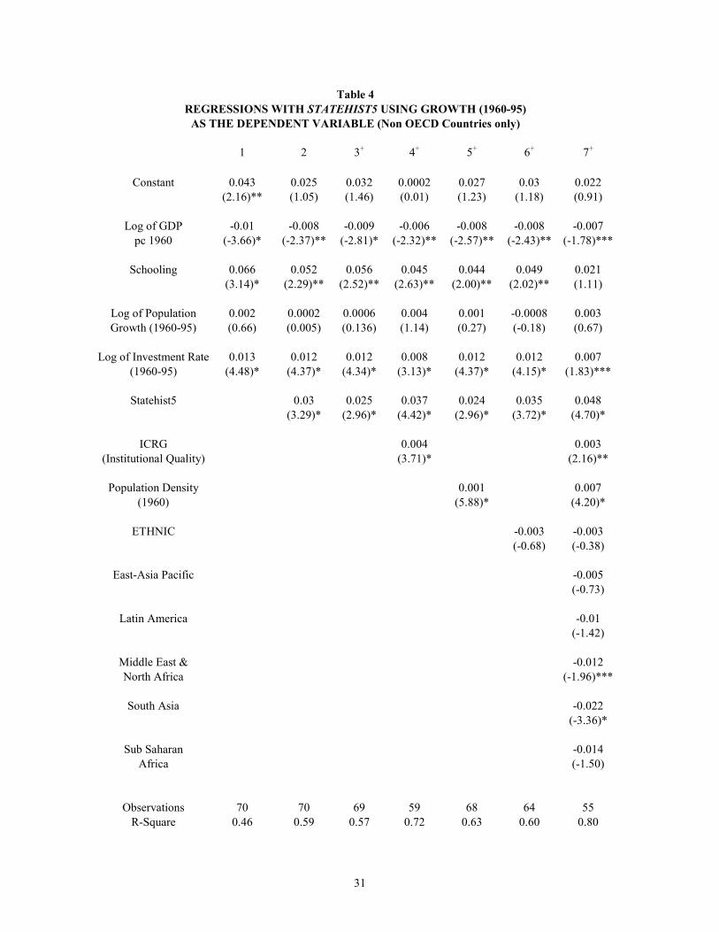
Conceivably, the relationships suggested by Table 3 hold only when the more
industrialized economies are included in the sample. An early state might account for
faster growth, in a global sample, but not greater relative success among developing
countries. To check, we re-estimated the regressions excluding the OECD countries.25
The results, shown in Table 4, are consistent with the pattern displayed in Table 3.
Indeed, the explanatory contribution of statehist5 is arguably even stronger here, for
adding it to the base regression for the developing country sample raises R-squared from
.46 to almost .59, raising the variation in growth rates that is explained by almost 13%.
What about income levels?
In addition to looking at growth regressions, one can also check whether
statehist5 helps to explain differences in income levels.26 This is interesting for two
reasons. First, ultimately what we care about is differences in average income levels since
they are a more relevant indicator of welfare than growth rates.27 Secondly, as noted
earlier in connection with Table 2, the correlation of statehist5 is clearly seen to be
increasing with income levels over time. This would suggest that more recent cross
sectional variances in income levels might be explained by statehist5, even after
controlling for other factors. Most of the work on income levels tries to decompose
differences in output per capita into differences in stocks of accumulable factors such as
physical and human capital and the residual total factor productivity. For example Hall
and Jones (1999) (henceforth HJ) find that differences in total factor productivity are
significantly more important in explaining differences in output per worker than are
conventional factors such as human capital and physical capital. Further, they find that
16
their measure of “social infrastructure” (henceforth SI) helps explain these output per
worker differences.
Table 5 examines whether statehist5, is a proximate determinant of economic
development.28 Included as control variables are the independent variables from Table 4
that can be viewed as sufficiently exogenous, plus one additional geographic variable,
latitude.29 While the results in column (1) suggest that statehist5 might have some
predictive power, the results in column (2), which repeats the same regression but
introduces SI as an additional control, do not support a significant role for statehist5.
While statehist5 is unlikely to be a proximate determinant of differences in
income, it may be a legitimate candidate to serve as a more fundamental determinant.
Given that most economic variables, which seek to explain differences in income levels,
will probably be endogenous to income levels themselves, statehist5 might also serve as
an instrument for such variables. Here, we explore how statehist5 performs as an
instrument for the SI variable used by Hall and Jones, given the commonalities in what
both variables claim to capture. As we have just observed, the introduction of SI robs
statehist5 of its predictive power in the levels equation of Table 5. At the same time, HJ
have rightly noted that SI is vulnerable to simultaneity bias. The correlation between
statehist5 and SI turns out to be 0.48. How does statehist5 compare with other
instruments for SI? Table 6a reports OLS regressions of SI on the four instruments used
by HJ—fraction of country’s population speaking one of Western Europe’s five main
languages (including English) (EURFRAC), the fraction speaking English (ENGFRAC),
the latitude and the logarithm of predicted trade share of an economy based on a gravity
model that only uses a country’s population and geographical features
(LOGFRANKFROM)—and statehist5.30 The table reports results when the sample
17
includes all countries and when it excludes OECD countries. As is apparent, statehist5 is
one of the most significant predictors of social infrastructure, making a strong case for its
use as an instrument.
Table 6b reports both OLS and generalized method of moments-instrumental
variable (GMM-IV) regression results for output per worker and SI. The fact that SI may
be measured incorrectly implies that OLS estimation would produce a coefficient that is
biased downwards. On the other hand the fact that output per worker itself may positively
affect SI implies that the OLS coefficient will be biased upwards. Column (1) reports the
OLS estimation and column (2) reports the GMM-IV estimation when statehist5 is not
included in the list of instruments. In keeping with HJ’s findings, the GMM-IV
coefficient is higher than the OLS coefficient suggesting that measurement error is the
more important of the two.31 Column (3) reports the GMM-IV results when statehist5 is
added to the list of instruments. As is apparent, the significance of social infrastructure is
increased, though the estimated coefficient declines. This suggests that adding statehist5
to the list of instruments probably helps lower measurement error. Also the p-values of
the overidentification test indicate that the null hypothesis that the instruments are
orthogonal to the error terms can be accepted.32
Conclusion
It is increasingly appreciated that an effective government can be an asset in the
struggle to achieve modern economic growth. There is also a growing body of research
suggesting that certain social preconditions may be as important a determinant of growth
performance as are economic policies and resource endowments. The findings of this
paper suggest that an early territory-wide polity and experience with large-scale
18
administration may make both for more effective government and for more rapid
economic growth. An early state may be associated with more rapid growth in part
because it is associated with greater ethnic homogeneity, a dense population, and higher
measured quality of government, but there is a significant further effect not accounted for
by these variables. These results may be viewed as lending support to the emphasis on
capacity-building and institutional quality in current programs to foster economic
development.
Over and above their policy implications, our findings may also contribute to a
better understanding of the effects of economic history on recent economic performance.
Although the industrial revolution that began in northwest Europe in the 18th Century did
not spread rapidly to early states remote from its point of origin, under late 20th Century
conditions less developed countries that had reached the state level of societal evolution
earlier than others were more successful in catching up with early developers. Because
European countries and Japan also resumed robust growth after the Second World War,
growth rates in the world as a whole during 1960-95 were strongly correlated with state
antiquity. Levels of development at the end of that period were correlated with state
antiquity, too, and the index of state antiquity helps to predict the social infrastructure
variable that Hall and Jones use to explain the cross-country output per worker
differences in 1988.
19
Appendix A
Antiquity of State (Statehist) Scores By Country and Region
Note: Statehist0, Statehist01, Statehist1, Statehist5, Statehist10 and Statehist50 are calculated by discounting half centuries at rates of 0, 0.1, 1, 5, 10 and 50%, respectively. Region Averages reflect 1960
Note: The correlation of 1 between statehist0 and statehist01 reflects a computer generated approximation.
23
Appendix C Examples of Statehist.
• Italy: The first four hundred years of Italy's history beginning in 1 C.E. can be
equated with Roman history. Thus Italy had an indigenous, comprehensive government until the fall of the Roman Empire, so that q1=q2=q3=1. From that point until unification in 1861, all of Italy's regions were part of governmental structures, most being locally based, so that q1=q2=1. These include the famous city-states and republics, as well as the territories that were part of the Holy Roman Empire. However, q3=0.75 for this period because Italy contained no single state controlling most of the present country’s territory. Due to Italy’s unification in 1861, both of the final two periods are treated as having q1=q2=q3=1. Multiplying q1xq2xq3x50 gives the following scores for the 50 year periods between each set of dates shown below:
• Mexico: During the first millennium and the outset of the second, agrarian village
societies began to emerge in what is now Mexico, but a general polity first emerged with the Aztecs, whose kingdom comprised around half of present day Mexico by about 1200. Hence, q1 = 0 for 0 – 1200, while q1 = q2 = 1 and q3 = 0.75 between 1200 and Spanish exploration in the 16th century. Between 1550 and 1600, the Aztec empire had already diminished in power and scope, but the Spanish conquerors had not reached the entire territory of Mexico, resulting in scores of q1=1, q2=0.5 and q3=0.75. By 1600, the Spanish had colonized most of Mexico, giving it a scores of q1 = 1, q2 = 0.5, q3 = 1. In the first half of the 19th century, Mexico gained independence. The value of q2 jumps from 0.5 to 1 during the course of this period, and we use the average value of 0.75. With full independence achieved, q1 = q2 = 1 between 1850 and 1950. Multiplying q1xq2xq3x50 gives the following scores for the 50 year periods between each set of dates shown below:
References Abramovitz, Moses, 1986, “Catching up, forging ahead, and falling behind,” Journal of Economic History, 46: 385-406. Acemoglu, Daron, Simon Johnson and James Robinson, 2001, “The Colonial Origins of Comparative Development: An Empirical Investigation,” American Economic Review 91 (5): 1369-1401. ___________________________________, 2002, “Reversal of Fortune: Geography and Institutions in the Making of the Modern World Income Distribution,” Quarterly Journal of Economics 117 (4): [in press]. Adelman, Irma and Cynthia T. Morris, 1967, Society, Politics and Economic Development. Baltimore: Johns Hopkins University Press. Alfaro, Laura, Areendam Chanda, Sebnem Kalemli-Ozcan and Selin Sayek, 2001, “FDI and Economic Growth: The Role of Local Financial Markets,” Harvard Business School Working Paper 2001-083. Aron, Janine, 1999, “Growth and Institutions: A Review of the Evidence,” unpublished paper, University of Oxford, May. Banks, Arthur, 1994, “Cross-National Time Series Data Archive,” Center for Social Analysis, SUNY Binghamton. Barro, Robert, 1991, “Economic Growth in a Cross-Section of Countries,” Quarterly Journal of Economics 106: 407-44. ___________ and Jong-Wha Lee, 1994, “Sources of Economic Growth,” Carnegie-Rochester Conference Series on Public Policy. Beck, Thorsten, R. Levine and N. Loayza, 2000, “Finance and the Sources of Growth,” Journal of Financial Economics, 58, 261—300 Boserup, Ester, 1965, Conditions of Agricultural Growth: The Economics of Agricultural Change Under Population Pressure. New York: Aldine. Burkett, John, Catherine Humblet and Louis Putterman, 1999, “Pre-Industrial and Post-War Economic Development: Is There a Link?” Economic Development and Cultural Change, 47 (3): 471-95.
25
Chanda, Areendam and Louis Putterman, 2000, “Economic Growth, Social Capability, and Pre-Industrial Development,” a report to the World Bank Africa Region Technical Families, Macroeconomics 2, October. Coleman, James, 1988, “Social Capital in the Creation of Human Capital,” American Journal of Sociology, 94: S95-S120. Dasgupta, Partha, 1998, “Economic Development and the Idea of Social Capital,” in P. Dasgupta and I. Seralgeldin, eds., Social Capital: Integrating the Economist’s and the Sociologist’s Perspectives. Washington, D.C.: The World Bank. Diamond, Jared, 1998, Guns, Germs and Steel: The Fates of Human Societies. New York: W. W. Norton. Easterly, William and Ross Levine, 1997, “Africa’s Growth Tragedy: Policies and Ethnic Divisions,” Quarterly Journal of Economics 112: 1203-1246. Frankel, Jeffrey A. and David Romer, 1999, “Does Trade Cause Growth?”, American Economic Review, 89(3): 379-99. Hall, Robert E. and Jones, Charles I., 1999, “Why Do Some Countries Produce So Much More Output per Worker than Others?” The Quarterly Journal of Economics, 114: 83-116. Kaufmann, Daniel, Aart Kraay and Pablo Zoido-Lobaton, 1999, “Governance Matters,” unpublished paper, The World Bank, August. Klenow, Peter J. and Andres Rodriguez-Clare, 1997, “The Neo-Classical Growth Revival in Economics: Has it Gone Too Far?” NBER Macroeconomics Annual, Cambridge and London: MIT Press, pages 73-103. Knack, Stephen and P. Keefer, 1995, “Institutions and Economic Performance: Cross Country Tests Using Alternative Institutional Measures,” Economics and Politics, 7:207-27. Knack, Stephen and P. Keefer, 1997, “Does Social Capital Have an Economic Payoff? A Cross-Country Investigation,” Quarterly Journal of Economics, 112:1251-1288. La Porta, Rafael, Florencio Lopez-de-Silanes, Andrei Shleifer, and Robert Vishny, 1997, “Legal Determinants of External Finance,”, Journal of Finance, 52: 1131-50. La Porta, Rafael, Florencio Lopez-de-Silanes, Andrei Shleifer, and Robert Vishny, 1998, “Law and Finance,” Journal of Political Economy, 106, 1113—1155 Levine, R., N. Loayza and T. Beck, 2000, “Financial Intermediation and Growth: Causality and Causes,” Journal of Monetary Economics, 46:1, 31—77
26
Levine, Ross and David Renelt, 1992, “A Sensitivity Analysis of Cross-Country Growth Regressions,” American Economic Review 82: 942-63. Loury, Glenn, 1977, A Dynamic Theory of Racial Income Differences, P.A. Wallace and A. Le Mund eds. Women, Minorities and Employment Discrimination, Lexington, MA: Lexington Books. Mankiw, Gregory N., David Romer and David N. Weil, 1992, A Contribution to the Empirics of Economic Growth, Quarterly Journal of Economics, Mauro, Paolo, 1995, “Corruption and Growth,” Quarterly Journal of Economics 110: 681-712. Narayan, Deepa, 1997, “Voices of the Poor: Poverty and Social Capital in Tanzania,” Environmentally and Socially Sustainable Development Studies and Monographs Series 20, The World Bank. Putnam, Robert, with Robert Leonardi and Raffaella Nanetti, 1993, Making Democracy Work : Civic Traditions In Modern Italy. Princeton, NJ: Princeton University Press. Putterman, Louis, 2000, “Can an Evolutionary Approach to Development Predict Post-War Economic Growth?” Journal of Development Studies (in press). Sachs, Jeffrey and Andrew Warner, 1997, "Sources of Slow Growth in African Economies," Journal of African Economies 6 (3): 335-76. Temple, Jonathan, 1998, Initial Conditions, Social Capital and Growth in Africa, Journal of African Economies, 7(3): 309-347. Temple, Jonathan and Paul A. Johnson, 1998, Social Capability and Economic Growth, Quarterly Journal of Economics, 113(3): 965-990. World Bank, 1997, World Development Report 1997: The State in a Changing World. Washington, D.C.: The World Bank
27
Table 1
Regional Averages of Statehist5 (Weighted by 1960 Population)
+ Hong Kong has been dropped from Regressions (3)-(7) Note: Numbers in parentheses are t statistics (calculated from heteroscedastic consistent standard errors). Schooling refers to secondary school enrollment ratio in 1960. Institutional Quality is as measured by the ICRG index. ETHNIC is the variable used in Easterly and Levine (1997) *= significant at .01 level; ** = significant at .05 level; *** = significant at .10 level
31
Table 4
REGRESSIONS WITH STATEHIST5 USING GROWTH (1960-95) AS THE DEPENDENT VARIABLE (Non OECD Countries only)
+ Hong Kong has been dropped from Regressions (3)-(7)
Note: Numbers in parentheses are t statistics (calculated from heteroscedastic consistent standard errors). Schooling refers to secondary school enrollment ratio in 1960. Institutional Quality is as measured by the ICRG index. ETHNIC is the variable used in Easterly and Levine (1997) *= significant at .01 level; ** = significant at .05 level; *** = significant at .10 level
33
Table 5 REGRESSIONS WITH STATEHIST5 USING LOG OF
OUTPUT PER WORKER (1988) AS DEPENDENT VARIABLE
(1) (2)
Constant 8.897 (14.78)*
8.558 (15.53)*
STATEHIST5 0.742 (1.85)***
0.194 (0.50)
ETHNIC -0.182 (-0.73)
-0.131 (-0.58)
Population Density
(1960) 0.041
(2.21)** 0.015 (0.84)
East-Asia Pacific -0.06
(-0.11) -0.493 (-0.93)
Latin America -0.099
(-0.17) -0.297 (-0.57)
Middle East & North Africa
0.473 (0.86)
0.192 (0.38)
North America 1.957
(2.87)* 0.646 (0.94)
South Asia -0.695
(-1.13) -0.619 (-1.11)
Sub-Saharan Africa -1.387
(-2.38)** -1.453
(-2.75)*
Latitude -0.011 (-3.02)*
-0.008 (-2.21)**
SOCINF 1.642
(4.31)*
Observations 93 93 R-Squared 0.79 0.81
Notes: Data for log output per worker and latitude is from Hall and Jones (1999). Numbers in parentheses are t statistics. ETHNIC is the variable used in Easterly and Levine (1997). SOCINF refers to “social infrastructure” in Hall and Jones (1999). *= significant at .01 level; ** = significant at .05 level; *** = significant at .10 level
34
Table 6a HALL-JONES SOCIAL INFRASTRUCTURE EQUATION WITH
STATEHIST5 AS AN ADDITIONAL INSTRUMENT Dependent variable: Social Infrastructure
(1) (2) All Countries Non OECD countries Constant 0.04
(0.33) -0.16 (-1.4)
ENGFRAC 0.21 (2.13)**
0.07 (0.58)
EURFRAC 0.14 (3.29)*
0.11 (2.51)**
LOGFRANKFOM 0.06 (1.64)
0.12 (3.80)*
LATITUDE 0.001 (0.58)
-0.004 (-3.04)*
Statehist5 0.49 (3.39)*
0.59 (3.92)*
Observations 101 77 R-Square 0.41 0.28 Notes: All data except statehist5 comes from Hall and Jones (1999). Both regressions exclude Hong Kong.
Table 6b
HALL-JONES PRODUCTIVITY EQUATION AFTER STATEHIST5 IS ADDED AS AN INSTRUMENT
Dependent Variable: Log of Output per Worker (1988)
(1) (2) (3) OLS GMM-IV
(excl. statehist5) GMM-IV
(incl. statehist5) SOCINF 3.27
(15.14) 4.90
(10.15) 4.77
(13.14) p-value of overidentification test - 0.22 0.31 Observations 101 101 101 Notes: SOCINF refers to “social infrastructure” in Hall and Jones (1999).Column (2) includes engfrac, eurfrac, logfrankrom and latitude as instruments. Column (3) also includes statehist5. The number in parenthesis for column (1) is the t-ratio and for columns (2) and (3) is the z-statistic. The p-values are for Hansen’s J-statistic. The R-Square for the OLS regression is 0.61. All regressions include a constant.
35
36
37
1 See World Bank, 1997, and sources cited therein. 2 See Janine Aron, 1999; Daniel Kaufmann, Aart Kraay and Pablo Zoido-Lobaton, 1999. 3 A discussion of economic accounts is provided by Dasgupta (1998). 4 For example, see La Porta, Lopez-de-Silanes, Shleifer and Vishny (1997), Beck, Levine and Loayza (2000), Levine, Loayza and Beck (2000), and Alfaro, Chanda, Kalemli-Ozcan and Sayek (2001). 5 We consulted with several experts on early states and were told that no such data series had been compiled. We are grateful to Gerhard Lenski for his suggestion that we construct our own index by consulting the Encyclopedia Britannica. We also thank Jared Diamond for putting us in touch with other scholars to discuss this index problem, and for his expression of enthusiasm about this project. 6 Although a few states date back well before the year 1, experience in the sufficiently remote past can be expected to have little or no current impact, and with a modest rate of discounting, this would have little effect on the measure we are constructing. 7 It might be preferable to score this first dimension along a continuum from countries with strong central governments or rulers to ones in which the central ruler has little power compared to formally subordinate local lords or chiefs, but to do so would require more information than is available to us. The exception is when our source identifies the top ruler as a “paramount chief” (e.g., Fiji). In this case, we assign a value of 0.75 for question 1. 8 Note that government by members of a group that migrated from another part of the world does not make the country a colony if the rulers are not directed by authorities in their place of origin. Thus, we count the British colonies of North America as colonies before 1776 but as independent afterwards, even though the region’s earlier inhabitants did not regain control when the colonists’ ties with the home country were severed. 9 We also gave a score of 0.75 for question 3 if there were several co-existing states in today’s region that covered the majority of the country (for example India before the Muslim invasions around 1200 or Italy between the fall of Rome and the formation of a nation state in the mid 19th century). 10 Specifically, to each of the 39 observations for a country we attached an exponent (1 + δ)-t, where 0 < δ < 1 functions like a discount rate, and t is the number of half centuries by which the period precedes 1901-1950 (for example, t = 1 for 1851-1900). At δ = .5, for example, the contribution to our index of having had an autonomous state over the whole territory from 1851 to 1900 is 50x(1.5)-1 = 33.33. 11 In statehist5, that is, δ of the previous note is equal to 0.05. At the 5% rate, the period 1000-1950 C.E. receives 71% of the overall weight in the index, versus 29% for the millennium 1-1000 C.E., assuming equal scores in each half century. At a 1% discount rate, the weights are 54% and 46%, respectively, while at a 10% discount rate, they are 86% and 14%. 12 These five indicators are used in Knack and Keefer (1995) followed widely by other studies including Sachs and Warner (1997) and Hall and Jones (1999). 13 Based on the assassination data used in Barro (1991). 14 Both variables are from Banks’ (1994) data set as used by Easterly and Levine. 15 Real GDP Per Capita in constant dollars (international prices, base year 1985) taken from the Global Development Network Growth Database.
38
16 Also, the relative disadvantage of some sub-Saharan African countries (with short state histories) may have become more apparent with the passage of time after independence because their per capita incomes circa 1960 may have been heavily influenced by colonial era investments that post-independence regimes were unable to maintain. 17 There is a significant negative correlation within the set of Latin American countries, which tends to cancel out the positive correlation for the rest of the developing world. It appears that Latin America behaves somewhat unlike other regions because Latin American countries with states and dense populations pre-dating European conquest experienced lower levels of social development and economic growth than Latin American countries formed from areas with sparse indigenous populations in which Europeans came to substantially outnumber indigenous people. This difference may actually be viewed as supporting the general trend since the longer state history of Europeans than of indigenous Americans was in a sense brought to the Americas with them, along with relative modernization and capacity for economic development. 18 We also examined the correlations between statehist5 and the origins of countries’ legal systems documented in La Porta et al (1998). We found that statehist5 was likely to be greater in countries that adopted the German and Scandinavian civil-laws. The correlations were 0.36 and 0.21 respectively. On the other hand the correlations with English common-law and French civil-law were –0.14 and –0.15 respectively. It is not clear, however, why a country with a longer experience with state level institutions should adopt a particular legal system. The high correlation with the German and Scandinavian legal system probably reflects the fact that countries which adopted those systems tend to have done better at enforcement of legal rules. And countries with higher values for statehist5 also do better in terms of institutional quality. Some of the measures of enforcement of legal rules used by La Porta et al (1998) are the same as the ICRG measures discussed earlier. 19 Unlike MRW, we use GDP per capita rather than GDP per worker for both the base and growth rate variables, and our human capital variable is simply the secondary school enrollment ratio. 20 As in the case of MRW, this is actually the log of (gpop6095+0.05), 0.05 being an estimate of the sum of the rate of depreciation of physical capital and TFP growth. 21 All data are from the World Development Indicators CD-ROM (2000). 22 Although Hong Kong was never a country in its own right, its economic autonomy has been such that it has been included as such in most cross-country growth studies. The value of the statehist measures is calculated for Hong Kong by coding years as part of China using q1 = q2 = q3 = 1 and years under British rule as q1 = q3 = 1, q2 = 0.5. The alternative of treating Hong Kong as a colony when ruled by China as well as when ruled by Britain is rejected because of Hong Kong’s longstanding Chinese culture and ultimate re-incorporation into that country. 23 All the remaining regressions in the table continue to omit Hong Kong. 24 These are World Bank dummies for East Asia-Pacific, Latin America, Middle East & North Africa, North America, South Asia, Sub-Saharan Africa and Western Europe. To avoid perfect collinearity the only region not included is Eastern and Central Europe. 25 OECD membership here excludes more recent members such as Mexico and Korea. Countries which are treated as OECD members and thus dropped in the next exercise are: Australia, Austria, Belgium, Canada, Switzerland, Germany, Denmark, Spain, Finland,
39
France, UK, Greece, Ireland, Iceland, Italy, Japan, Netherlands, Norway, New Zealand, Portugal, Sweden, Turkey, United States. Luxembourg is also a part of this sample but does not have a value for Statehist5. 26 We are grateful to an anonymous referee for suggesting this exercise. 27 The literature has begun to reflect this change in focus. See for example Klenow and Rodriguez-Clare (1998) in addition to Hall and Jones (1999). 28 The entire exercise that follows excludes Hong Kong from the sample. 29 In a regression with the level of income as the dependent variable, entering almost any economic variable e.g. the investment rate, schooling enrollment ratios, population growth rates, etc, as a control, would be highly susceptible to the simultaneity bias problem. The latitude variable is used as a predictor of social infrastructure by Hall and Jones. 30 The predicted trade share variable comes from Frankel and Romer (1999). All data for this exercise except statehist5 was downloaded from Charles Jones’ website: http://elsa.berkeley.edu/users/chad/HallJones400.asc . 31 HJ use a simple IV estimator. What we use is the GMM-IV estimator which allows for heteroscedasticity of an unknown form. 32 The results are robust when the sample is limited to non-OECD countries.