Supplemental Online Materials (SOM) for Balbus et al. Health Co-benefits of Specific U.S. Climate Activities Climate Change MS#4772 Appendix A: Fleet turnover analysis The magnitude of co-benefits achieved from enhancing the fuel economy of the light-duty and heavy-duty vehicle fleet strongly depends on whether new or old vehicles are replaced. Historically, fuel economy regulations have focused on new vehicle requirements due to the difficulties and cost associated with retrofitting or early replacement of used vehicles. Given recent changes to PM 2.5 and NO x emission regulations for cars and especially trucks, a GHG reduction policy focusing exclusively on new vehicles would have significantly less co-benefits than one that required replacement of older vehicles. For example, Figure A1 shows projected relative emission factors (g PM 2.5 / g fuel) and relative fuel-use by model year of cars (top) and trucks (bottom). One key difference between the light-duty and heavy-duty vehicle sectors is that heavy-duty trucks are operated for longer than light-duty vehicles, so the total fleet average emissions for cars respond to reduced new vehicle emission regulations in a shorter time frame than trucks. We estimate the reduction of PM 2.5 emissions from fuel economy improvements in new vehicles starting in 2015 by holding emissions per fuel burned from model years before 2015 constant and applying a factor to fuel-use for each future model year starting in 2015. We then weight the model year emission factor by the relative fuel use expected from each model year (model year % of vehicle fleet * model year % of total miles driven) and sum to find an average fleet emission factor for a future year. The relative age distribution of vehicles is assumed to stay constant over time and is based on separate age distributions for light and heavy-duty vehicles reported by Davis et al. (2011). 1
Transcript
Supplemental Online Materials (SOM) forBalbus et al. Health Co-benefits of Specific U.S. Climate
Activities Climate Change MS#4772
Appendix A: Fleet turnover analysis
The magnitude of co-benefits achieved from enhancing the fuel economy of the light-duty and heavy-duty vehicle fleet strongly depends on whether new or old vehicles are replaced. Historically, fuel economy regulations have focused on new vehicle requirements due to the difficulties and cost associated with retrofitting or early replacement of used vehicles. Given recent changes to PM2.5 and NOx emission regulations for cars and especially trucks, a GHG reduction policy focusing exclusively on new vehicles would have significantly less co-benefits than one that required replacement of older vehicles. For example, Figure A1 shows projected relative emission factors (g PM2.5/ g fuel) and relative fuel-use by model year of cars (top) and trucks (bottom). One key difference between the light-duty and heavy-duty vehicle sectors is that heavy-duty trucks are operated for longer than light-duty vehicles, so the total fleet average emissions for cars respond to reduced new vehicle emission regulations in a shorter time frame than trucks.
We estimate the reduction of PM2.5 emissions from fuel economy improvements in new vehicles starting in 2015 by holding emissions per fuel burned from model years before 2015 constant and applying a factor to fuel-use for each future model year starting in 2015. We then weight the model year emission factor by the relative fuel use expected from each model year (model year % of vehicle fleet * model year % of total miles driven) and sum to find an average fleet emission factor for a future year. The relative age distribution of vehicles is assumed to stay constant over time and is based on separate age distributions for light and heavy-duty vehicles reported by Davis et al. (2011). Emission factors (emissions/g fuel were converted from grams per brake horsepower-hour (gbhp-hr)) are simply based on the allowable emission limit for each model year depending on the regulations at the time (EPA maintains a history of emission regulations, see for example: http://www.epa.gov/otaq/standards/allstandards.htm). By comparing the future fleet emission factors we can find the expected magnitude of PM2.5 reductions from fuel economy improvements to new vehicles scenarios.
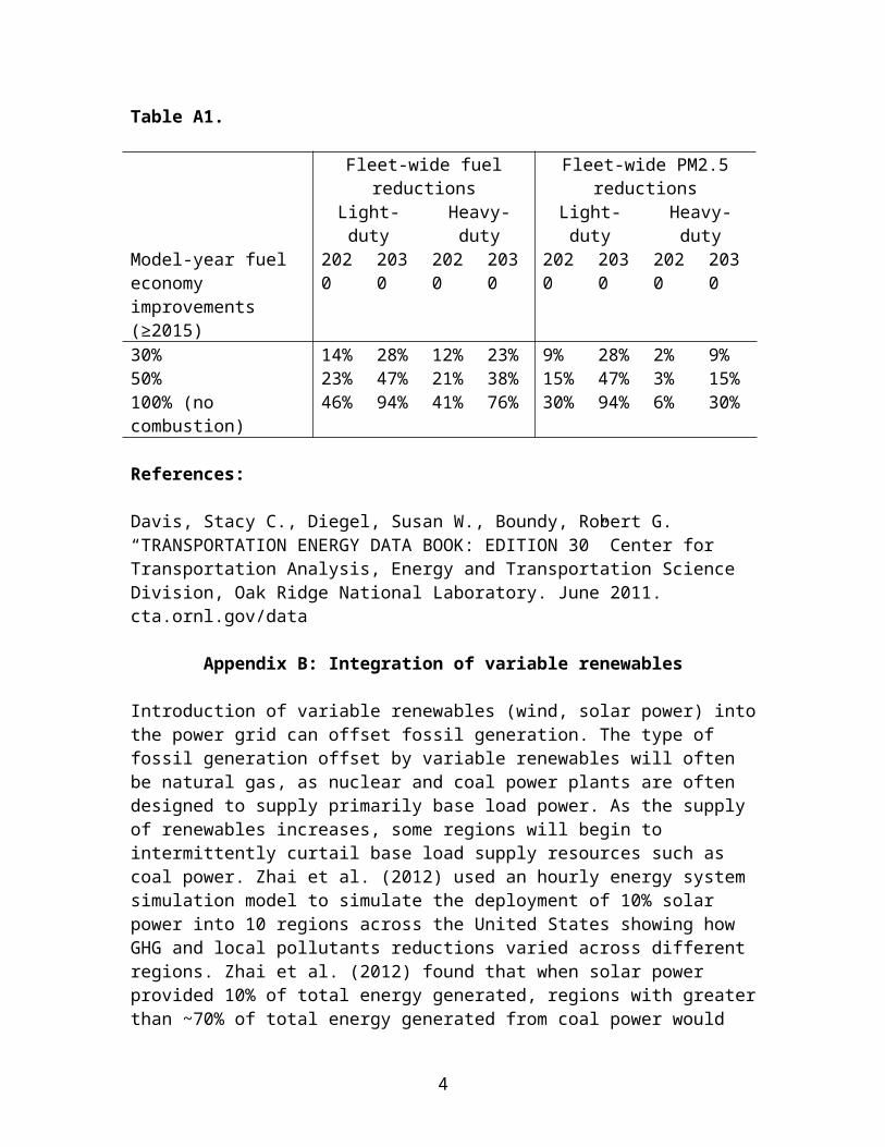
Table A1 shows expected PM2.5 reductions from 30, 50 and 100% fuel economy improvements to new vehicles beginning in 2015. Table A1
1
indicates that by 2030, a 30% fuel economy improvement for new cars starting in 2015 would yield 28% fleet-wide fuel savings and achieve a 23% reduction in PM2.5 emissions from cars. By 2030 a 30% fuel economy improvement for new trucks starting in 2015 would yield 23% fleet-wide fuel savings but only achieve a 9% reduction in PM2.5 emissions from trucks. Table A1 indicates that requiring new trucks to improve fuel economy starting in 2015 would achieve only marginal co-benefits by 2020. These results show that in order to realize co-benefits from a fuel economy program for heavy-duty trucks a policy must drive early replacement of older trucks as opposed to simply increasing new vehicle fuel economy standards.
Davis, Stacy C., Diegel, Susan W., Boundy, Robert G. “TRANSPORTATION ENERGY DATA BOOK: EDITION 30” Center for Transportation Analysis, Energy and Transportation Science Division, Oak Ridge National Laboratory. June 2011. cta.ornl.gov/data
Appendix B: Integration of variable renewables
Introduction of variable renewables (wind, solar power) into the power grid can offset fossil generation. The type of fossil generation offset by variable renewables will often be natural gas, as nuclear and coal power plants are often designed to supply primarily base load power. As the supply of renewables increases, some regions will begin to intermittently curtail base load supply resources such as coal power. Zhai et al. (2012) used an hourly energy system simulation model to simulate the deployment of 10% solar power into 10 regions across the United States showing how GHG and local pollutants reductions varied across different regions. Zhai et al. (2012) found that when solar power provided 10% of total energy generated, regions with greater than ~70% of total energy generated from coal power would see reductions in emissions of SO2, NOx, and PM2.5 from coal power generation. However, the simulation indicated that regions generating less than 60% of their energy from coal power would see little reduction in coal power use with the introduction of 10% solar power generation. The 60-70% threshold for reducing coal power generation discussed above is reduced if a region has energy generated from nuclear power as well. Based on Zhai et al. (2012) we identify regions of the U.S. where coal power generation would be sensitive to 10% penetration of variable renewables (Figure B2). Based on the generation mix described for NERC subregion tabulated
4
by EPA in eGRID (EGRID 2012), much of the area from the Dakota’s through to West Virginia has a prior generation mix similar to the generation mix that was identified by Zhai et al. (2012) to show reductions in emissions of pollutants and GHG associated with coal power generation. Areas with lower levels of coal generation, such as Colorado or Texas would see little reductions in coal use from the introduction of 10% variable renewables. The states highlighted in Figure B2 account for roughly 60% of national net coal generation in the U.S. in 2011, (EIA 2013).
Figure B2. NERC sub-regions with areas highlighted where prior generation mix would likely allow for reduced coal power emissions from the integration of 10% variable renewables on an energy basis. (Sub-regions are mapped from EPA’s EGRID 2012).
References:EIA, “Electric Power Annual 2011” (2013). Independent Statistics and Analysis, US Energy Information Administration.EGRID 2012, “eGRID2012 Version 1.0 Year 2009 Summary Tables”, US EPA, created April 2012. http://www.epa.gov/cleanenergy/energy-resources/egrid/index.html.Zhai, P., Larsen, P., Millstein, D., Menon, S., Masanet, E.: 2012, ‘The potential for avoided emissions from photovoltaic electricity in the United States’, Energy 47, 443-450 http://dx.doi.org/10.1016/j.energy.2012.08.025.
Table C1 describes the combinations of wedge activities used and the estimated potential reductions in activity. The reductions become more pronounced in 2060 as the amount of remaining CO2 emitted becomes appreciably smaller.
As an example, Figure C1 shows the change in the required reduction of coal plant energy consumption as the number of combined wedges increases. The reductions are shown for wedge 6 (increased efficiency of baseload coal plants), combination wedge 3 (increased coal plant efficiency combined with two wedges of zero-carbon coal plant substitutions—wedges 8, 9 or 10) and combination wedge 4 (combination wedge 3 with increased building efficiency included—wedges 4 and 5). As one moves from wedge 6 to combination wedge 3 to combination wedge 4, the amount of coal plant efficiency required increases, and the degree of increase becomes stronger toward later years.
6
TABLE C1 Potential Reductions for Combined Wedge Activities
Wedge Activities
Number of Total Wedg
es Activity Units
Reduction in Activity
2020 2030
2060
Transportation1. Combine
increased light-duty fuel efficiency and reduction of light-duty vehicle miles traveled
2.0
Vehicle efficiency
Million barrels/d
ay12% 21% 36
%
Vehicle-miles
travelled
Billion miles/ye
ar12% 21% 36
%
Buildings2. Combine
increased electric end-use and direct fuel building efficiency
2.0
Electrical efficiency
Terawatt-hours/
year8% 13% 26
%
Direct fuel
efficiencyQuads/
year 23% 44% 98%
Power Plants3. Combine
increased efficiency of baseload coal plants and two zero-carbon coal substitutions
3.0
Coal plant
efficiencyQuads/
year 7% 11% 25%
Coal plant
substitutions (per wedge)
Terawatt-hours/
year7% 11% 25
%
Buildings and Power Plants
4. Combine efficient buildings wedges and all power plant wedges
5.0
Building electrical efficiency
Terawatt-hours/
year9% 17% 49
%
Building direct fuel
efficiency
Quads/year 23% 44% 98
%
Coal plant
efficiencyQuads/
year 7% 12% 34%
Coal plant
substitutions (per wedge)
Terawatt-hours/
year7% 12% 32
%
7
8
FIGURE C1 Comparison of Reduction in Coal Plant Capacities Among Individual and Combination Wedges
Health impact functions relate changes in health outcomes to changes in ambient PM2.5 concentrations. Health impact functions typically consist of four components: a concentration-response (CR) function derived from epidemiological studies, a baseline incidence rate for the health effect of concern, the affected population, and the projected change in ambient PM2.5 concentrations. The majority of the studies we used to estimate CR functions assume that the relationship between adverse health outcomes and PM2.5 pollution is best described as log-linear, where the natural logarithm of the health response is a linear function of PM2.5 concentrations. The change in number of outcomes (𝐸) of health endpoint 𝐽 when ambient concentrations (𝐶) of PM2.5 change can be given by:
∆ EJ=[exp (βJ×∆C )−1 ]×E0J× PopJ, (1)
where βJ is the CR coefficient of health endpoint J and E0J is the baseline incidence rate of health endpoint J in the affected population, PopJ . Because βJ is small, Eq.1 can be linearized and expressed as the following:
∆ E J=βJ× E0J×∆C ×PopJ (2)
9
The following subsections describe the methods and sources used to define the health impact function elements, along with the uncertainties considered in the analysis.
We use the concept of intake fractions to calculate the exposure concentration of PM2.5 associated with a given amount of emissions in the year 2020. An intake fraction is the fraction of PM2.5 released from a source (such as motor vehicles or power plants) that is eventually inhaled or ingested by a population. It is dimensionless and can be defined as the ratio of the time-averaged inhalation rate to the time-averaged emission rate (Levy et al. 2002). Mathematically, the intake fraction takes the following form:
iF=∑i=1
N
Pi×C i×BR
Q , (3)
where Pi is the population at location i, C i is the incremental concentration (µg/m3) of pollutant at location i, BR is the breathing rate (m3/day), Qis the pollutant emission rate (µg/day), and N is the number of receptor sites.
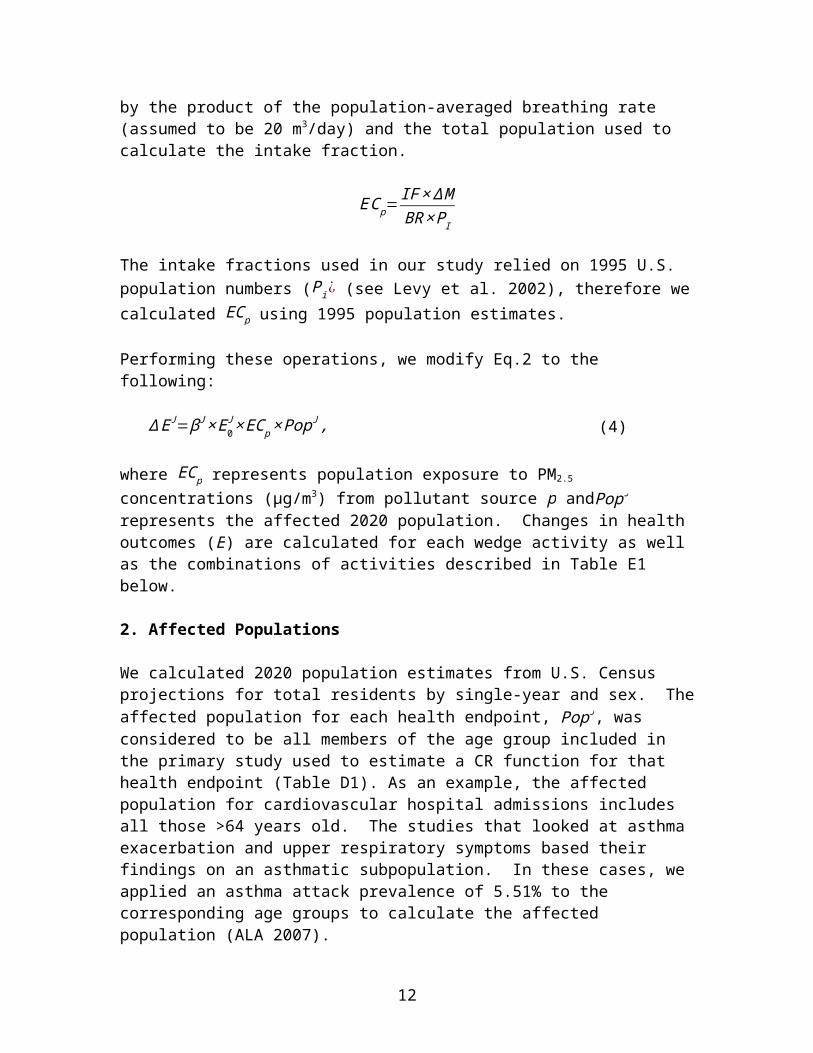
We can quantify the average population exposure concentration (EC p) in units of µg/m3 resulting from PM2.5 emissions by multiplying the intake fraction by the expected change in PM2.5 emissions in units of µg/day (M ¿ and dividing by the product of the population-averaged breathing rate (assumed to be 20 m3/day) and the total population used to calculate the intake fraction.
EC p=IF ×∆MBR×P I
The intake fractions used in our study relied on 1995 U.S. population numbers (Pi ¿ (see Levy et al. 2002), therefore we calculated EC p using 1995 population estimates.
Performing these operations, we modify Eq.2 to the following:
∆ EJ=βJ×E0J×EC p×PopJ , (4)
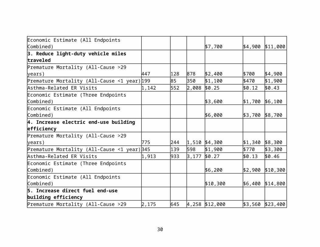
where EC p represents population exposure to PM2.5 concentrations (µg/m3) from pollutant source p andPopJrepresents the affected 2020 population. Changes in health outcomes (E) are calculated for each wedge activity as well as the combinations of activities described in Table E1 below.
10
2. Affected Populations
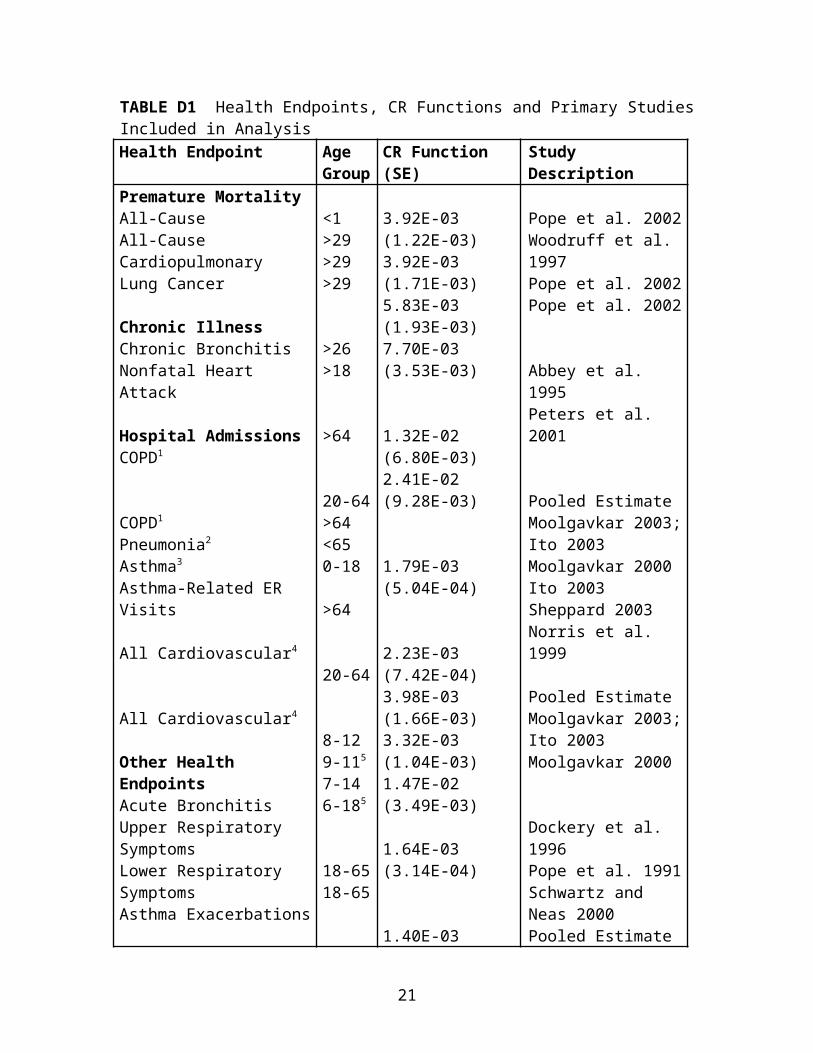
We calculated 2020 population estimates from U.S. Census projections for total residents by single-year and sex. The affected population for each health endpoint, PopJ, was considered to be all members of the age group included in the primary study used to estimate a CR function for that health endpoint (Table D1). As an example, the affected population for cardiovascular hospital admissions includes all those >64 years old. The studies that looked at asthma exacerbation and upper respiratory symptoms based their findings on an asthmatic subpopulation. In these cases, we applied an asthma attack prevalence of 5.51% to the corresponding age groups to calculate the affected population (ALA 2007).
3. Baseline Health Incidence Rates
Baseline incidence rates for each health endpoint are needed to translate the relative risk of health effect J, derived from the CR function, to the absolute change in health effect, or the number of avoided cases per year. Table D2 provides a summary of baseline incidence rates and their sources.
Whenever possible, average baseline incidence rates for different age groups were determined from national survey data. For those endpoints with survey data, we chose the most recent incidence rate available to include in the analysis. We also generated the last 5 years of survey data to assess trends and ensure comparability of incidence rate estimates between years.
Age- and cause-specific mortality data were generated from the Centers for Disease Control and Prevention’s (CDC) internet database, CDC Wonder (CDC 2008). CDC derives incidence rates from U.S. death records and Census postcensal population estimates and outputs mortality rates for specified age ranges, locations, and ICD10 codes. Because our study outcomes presented ICD9 codes for mortality-related diseases, we converted ICD9 to ICD10 codes and generated mortality rates for the latest year available in CDC Wonder (2004). It should be noted that CDC Wonder generates age groupings in 10-year intervals. To estimate mortality rates for ages >29, we scaled the 25-34 year age group by half, and by assuming that death rates were uniform across all ages in the 10-year age group, we calculated population-weighted mortality rates for the scaled age groups.
11
Respiratory- and cardiovascular-related hospital admission incidence rates for 2005 were determined from CDC’s National Hospital Discharge Survey (NHDS), which gathers data from nonfederal short-stay hospitals across the U.S. (CDC 2005). Nonfatal heart attack incidence was also ascertained from 2005 NHDS data. Per EPA methodology, we multiplied the incidence data by 0.93 based on a Rosamond (1999) estimate that 7% of hospitalized patients die within 28 days.
Emergency-room visits for asthma were estimated from the CDC National Hospital Ambulatory Care Survey as presented in the CDC report, CDC National Surveillance for Asthma --- United States, 1980—2004 (CDC 2007). CDC presented data for <18, while our population of interest includes 18, so the incidence estimates may be conservative.
Acute bronchitis, work-loss days, and minor-restricted activity day incidence rates were determined from CDC’s National Health Interview Survey (NHIS). The last year acute bronchitis and minor restricted activity days were included in the NHIS was 1996 (CDC 1996). For acute bronchitis, incidence rates are presented for the age range 5-17, which most likely represents an overestimate. The incidence rate for work loss days was taken from the 2006 NHIS (CDC 2006).
For other endpoints, the only incidence data for the population of concern comes from the primary study itself. In these cases, the incidence in the study population is assumed to represent the incidence in the national population.
4. Economic Valuation of Health Endpoints
To value the benefits of reduced premature mortality rates, EPA used the VSL approach. EPA’s guidance provided a number of VSL options, ranging from 5.5-6.3 million dollars. We chose a VSL of 6.3 million dollars because it is the primary value used by EPA in its BenMap software (EPA 2008). WTP estimates were used to value reductions in cases of chronic bronchitis, acute bronchitis, upper and lower respiratory symptoms, asthma exacerbations, and minor restricted activity days. WTP estimates are generally not available for hospital admissions, and for these health endpoints, cost-of-illness (COI) valuation estimates are used. COI estimates reflect direct expenditures, medical and opportunity costs, but do not take into account the value associated with reduced pain and suffering, and are thus likely underestimates. Finally, work-loss-days were valued
12
according to the daily median wage in the U.S. Table D3 summarizes the types and sources of economic valuations used in the analysis.
To calculate the monetary benefits associated with reductions in adverse health outcomes, the economic valuation estimate was multiplied by the change in health effect (E J¿ . Results given are in 2008 US Dollars. Because the economic values obtained from the EPA were in 2000 USD, we updated them to 2008 USD by adjusting by the increase in the US Consumer Price Index for all Urban Consumers (CPI-U) from 2000 to December, 2008 (USDOL, 2008). Economic benefits due to reductions in adverse health outcomes were calculated for each wedge activity as well as different combinations. We note that these economic benefits do not incorporate the costs associated with development and implementation of wedge activities – they reflect gross and not net economic benefits.
5. Uncertainty Analysis
The change in health and economic outcomes associated with different wedge activities for the year 2020 depends on five main analysis inputs: change in PM2.5 emissions, CR functions, baseline health incidence rates, 2020 population projections, and intake fractions (to relate emissions of PM2.5 to concentrations). Each is uncertain to a different degree and we characterized the total uncertainty surrounding final health and economic outcomes through Monte Carlo uncertainty propagation of the inputs. In Monte Carlo simulations, inputs generated through random sampling from probability distributions are used to characterize uncertainty in the outputs. Assignment of a distribution to each input was based on the best available information. For example, CR functions were assumed to be normally distributed, with a mean and standard error as reported in the primary study. When no distribution information was available, inputs were assumed to be uniformly distributed with a maximum and minimum of ± 50% the base estimate. Crystal Ball 7.3.1 was used to carry out the health and economic benefits analysis.
Table D4 describes the distributions assigned to each input and their sources. The final outputs were generated along with their standard deviations and 5th and 95th percentiles. In addition to Monte Carlo uncertainty propagation, we conducted sensitivity analyses to test the effect of alternative emissions scenarios on the final estimates. We performed an alternative analysis in which results for 2030 were moved forward to 2020 to reflect that some technologies included in the analysis are cost-beneficial or easily implemented; therefore, it is possible that the initial pace of implementation could be more rapid.
13
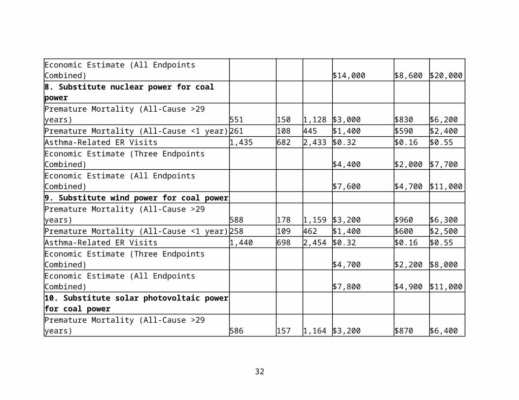
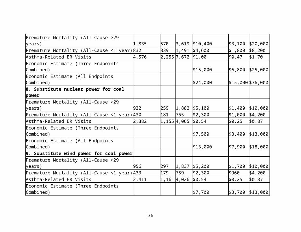
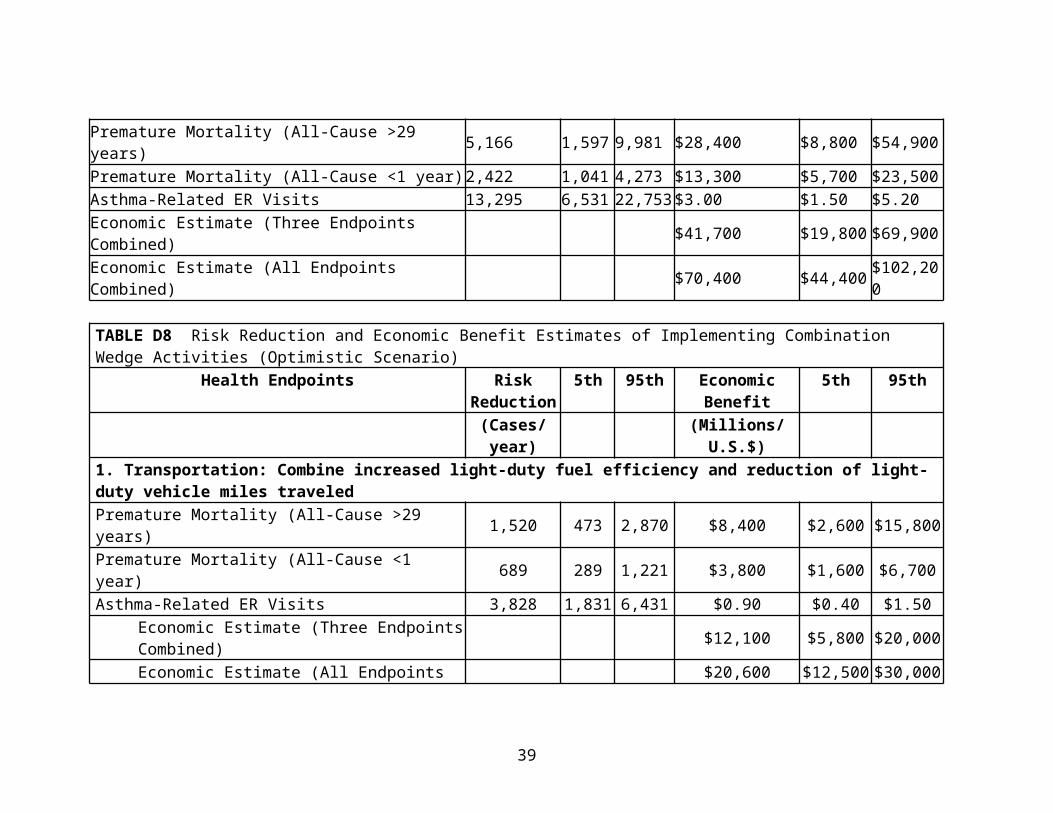
Results are shown in Table D5 through Table D8.
ReferencesAbbey, D. E., Hwang, B. L., Burchette, R. J., Vancuren, T., and Mills, P. K.: 1995, 'Estimated long-term ambient concentrations of PM(10) and development of respiratory symptoms in a nonsmoking population', Arch Env Health. 50(2): 139-152.
ALA (American Lung Association): 2007, Trends in Asthma Morbidity and Mortality, Epidemiology & Statistics Unit, Research and Program Services, Washington DC.
CDC (Centers for Disease Control and Prevention): 1996, National Health Interview Survey, 1996. Available online: http :// www . cdc . gov / nchs / nhis . htm [Accessed October 27, 2008].
CDC (Centers for Disease Control and Prevention): 2005, National Hospital Discharge Survey. Available online: http :// www . cdc . gov / nchs / about / major / hdasd / nhds . htm [Accessed October 27, 2008].
CDC (Centers for Disease Control and Prevention): 2006, National Health Interview Survey, 2006. Available online: http :// www . cdc . gov / nchs / nhis . htm [Accessed October 27, 2008].
CDC (Centers for Disease Control and Prevention): 2007, National Surveillance for Asthma --- United States, 1980—2004. MMWR: Surveillance Summaries. 56(SS08); 1-14; 18-54. Available online: http :// www . cdc . gov / mmwr / preview / mmwrhtml / ss 5608 a 1. htm [Accessed October 27, 2008].
CDC (Centers for Disease Control and Prevention): 2008, CDC Wonder. Compressed Mortality File: Underlying Cause-of-Death. Available online: http :// wonder . cdc . gov / mortSQL . html [Accessed October 27, 2008].
Chen, C., Wang, B., Fu, Q., Green, C. and Streets, D. G.: 2006, 'Reductions in emissions of local air pollutants and co-benefits of Chinese energy policy: A Shanghai case study', Energy Policy. 34, 754-762.
Chen, C., Wang, B., Huang, C., Zhao, J., Dai, Y., and Kan, H.: 2007, 'Low-carbon energy policy and ambient air pollution in Shanghai, China: A health-based economic assessment', Sci Total Environ. 373, 13–21
14
Davis, D. L. and Working Group on Public Health and Fossil Fuel Combustion.: 1997, 'Short-term improvements in public health from global-climate policies on fossil-fuel combustion: an interim report', Lancet. 350, 1341-1349.
Davis, D. L., Krupnick, A., and McGlynn, G.: 2000, Ancillary benefits and costs of greenhouse gas mitigation: An overview. Available from: http :// www . airimpacts . org / documents / local / M 00005776. pdf
Dockery, D. W., Cunningham, J., Damokosh, A. I., Neas, L. M., Spengler, J. D., Koutrakis, P., Ware, J. H, Raizenne, M., and Speizer, F. E.: 1996, 'Health effects of acid aerosols on North American children-respiratory symptoms', Environ Health Perspect. 104(5), 500-505.
EPA (U.S. Environmental Protection Agency): 2008, BenMap: Environmental benefits mapping and analysis program. User’s Manual Appendices. Prepared for Office of Air Quality Planning and Standards. Prepared by Abt Associates.
Ito, K.: 2003. Associations of particulate matter components with daily mortality and morbidity in Detroit, Michigan. In Revised Analyses of Time-Series Studies of Air Pollution and Health. Special Report. Health Effects Institute, Boston, MA.
Moolgavkar, S. H.: 2000, 'Air pollution and hospital admissions for diseases of the circulatory system in three U.S. metropolitan areas', J Air Waste Manage. 50, 1199-1206.
Moolgavkar, S. H.: 2003, Air pollution and daily deaths and hospital admissions in Los Angeles and Cook counties. In Revised Analyses of Time-Series Studies of Air Pollution and Health. Special Report. Boston, MA: Health Effects Institute.
Norris, G., Young Pong, S. N., Koenig, J. Q., Larson, T. V., Sheppard, L., and Stout, J. W.: 1999, 'An association between fine particles and asthma emergency department visits for children in Seattle', Environ Health Perspect. 107(6), 489-493.
Ostro, B. D.: 1987, 'Air pollution and morbidity revisited: A specification test', JEnviron Econ Managt. 14, 87-98.
Ostro, B. D. and Rothschild, S.: 1989, 'Air pollution and acute respiratory morbidity: An observational study of multiple pollutants', Environ Res. 50, 238-247.
15
Ostro, B., Lipsett, M., Mann, J., Braxton-Owens, H., and White, M.: 2001, 'Air pollution and exacerbation of asthma in African-American children in Los Angeles', Epidemiology. 12(2), 200-208.
Peters, A., Dockery, D. W., Muller, J. E., and Mittleman, M. A.: 2001, 'Increased particulate air pollution and the triggering of myocardial infarction', Circulation. 103, 2810-2815.
Pope, C. A., III, Dockery, D. W., Spengler, J. D., and Raizenne, M. E.: 1991, 'Respiratory health and PM10 pollution: A daily time series analysis', Am Rev Resp Dis. 144, 668-674.
Pope, C. A., III, Burnett, R. T., Thun, M. J., Calle, E. E., Krewski D., Ito, K., and Thurston, G. D.: 2002. 'Lung cancer, cardiopulmonary mortality, and long-term exposure to fineparticulate air pollution', J Am Med Assoc. 287, 1132-1141.
Rosamond, W., Broda, G., Kawalec, E., Rywik, S., Pajak, A., Cooper, L., and Chambless L.: 1999, 'Comparison of medical care and survival of hospitalized patients with acute myocardialinfarction in Poland and the United States', Am J Cardiol. Vol. 83(8), 1180-1185.
Schwartz, J. and Neas, L. M.: 2000, 'Fine particles are more strongly associated than coarse particles with acute respiratory health effects in school children', Epidemiology. 11, 6-10.
Schwartz, J., Dockery, D. W., Neas, L. M., Wypij, D., Ware, J. H., Spengler, J. D., Koutrakis, P., Speizer, F. E., and Ferris, B. G. Jr.: 1994, 'Acute effects of summer air pollution on respiratory symptom reporting in children', Am J Respir Crit Care Med. 150, 1234-1242.
Sheppard, L.: 2003, 'Ambient air pollution and nonelderly asthma hospital admissions in Seattle, Washington, 1987-1994', In Revised Analyses of Time-Series Studies of Air Pollution and Health. Special Report. Boston, MA: Health Effects Institute.
USDOL (United States Department of Labor): 2008, Consumer Price Index for all Urban Users. Available online: ftp :// ftp . bls . gov / pub / special . requests / cpi / cpiai . txt [Accessed January 16, 2009].
Vedal, S., Petkau, J., White, R., and Blair, J.: 1998, 'Acute effects of ambient inhalable particles in asthmatic and nonasthmatic children', Am J Resp Crit Care Med. 157(4), 1034-1043.
16
West, J, Fiore, A., Horowitz, L., and Mauzerall, D.: 2006, 'Global health benefits of mitigating ozone pollution with methane emission controls', P Natl Acad Sci USA. 103, 3988-3993.
Woodruff, T.J., Grillo, J., and Schoendorf, K.C.: 1997, 'The relationship between selected causes of postneonatal infant mortality and particulate air pollution in the United States', Env Health Perspect. 105(6), 608-612.
17
TABLE D1 Health Endpoints, CR Functions and Primary Studies Included in AnalysisHealth Endpoint Age
GroupCR Function (SE)
Study Description
Premature MortalityAll-CauseAll-CauseCardiopulmonaryLung Cancer
Other Health EndpointsAcute BronchitisUpper Respiratory SymptomsLower Respiratory SymptomsAsthma ExacerbationsWork Loss DaysMinor Restricted Activity Days
Other Health EndpointsAcute BronchitisUpper Respiratory SymptomsLower Respiratory SymptomsAsthma ExacerbationsWork Loss DaysMinor Restricted Activity Days
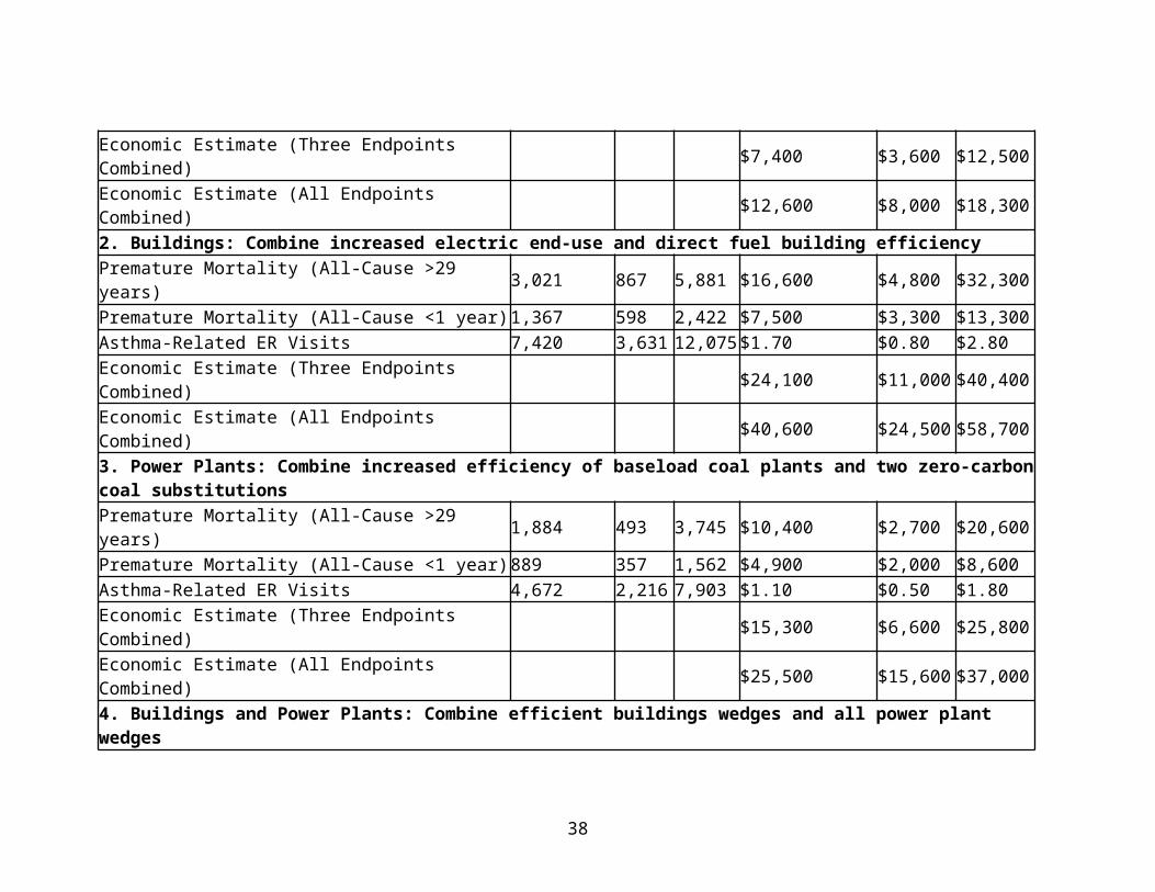
Because several wedges may reduce emissions from the same source but through different means, we evaluated specific combinations. The results of these combinations for the baseline and rapid implementation scenarios are in Table E1. Benefits in the “optimized” scenario were at least 1.5 times greater than the “baseline” scenario.
TABLE E1 Risk Reduction and Economic Benefit Estimates of Implementing Combination Wedge Activities
Economic Benefit(All Endpoints
Combined)(Millions/U.S.$)
Health Endpoints Baseline Scenari
o
Optimistic
Scenario1. TransportationCombine increased light-duty fuel efficiency and reduction of light-duty vehicle miles traveled
$12,600 $20,600
2. BuildingsCombine increased electric end-use and direct fuel building efficiency
$40,600 $74,700
3. Power PlantsCombine increased efficiency of baseload coal plants and two zero-carbon coal substitutions
$25,500 $39,900
4. Buildings and Power PlantsCombine efficient buildings wedges and all power plant wedges
$70,400 $124,000
2. Range of abatement costs for wedge activities
33
To place our calculated gross economic health benefits in context, estimated implementation costs for wedge activities from the recent literature (Creyts et al., 2007; IEA, 2009; NETL, 2010; Sovacool, 2011; EPA, 2012; Feldman et al., 2012; EIA, 2013) are summarized in Table E2 below.
3. Critique
In carrying through the analysis to the economic valuation of reduced adverse health outcomes, a number of critical assumptions and methodological choices were made. First, this analysis compares the health co-benefits associated with one wedge of CO2 reduction, rather than attempting to assess probable or maximum feasible implementation of each specific technological solution. Thus, ratios of health to CO2 reduction benefits can be compared among options, but the analysis is not intended to predict the likely magnitude of total health benefits associated with climate policies. A second critical assumption was the proportional reduction of conventional air pollutants and CO2. This assumption is likely to be invalid to varying degrees for the different solutions. For example, vehicle fuel efficiency does not correlate with vehicle pollutant emissions, as catalytic converters and other technologies can control emissions to a specified level of control regardless of fuel efficiency. The same is to some extent true for coal-fired power plant emissions, while solutions involving decreased vehicle miles would be expected to produce more proportional reductions.
Because our analysis assessed relative differences among reductions from specific sources, a method of estimating population-level exposures based on specific source reductions in primary pollutant emissions was necessary. We chose intake fractions as an initial approach in order to provide a computationally simple yet still science-based way of estimating dispersion of emissions. The use of intake fractions involves several major assumptions, including spatially uniform reduction of emissions, continued validity of distribution of sources and dispersion modeling upon which the intake fractions were originally based for 2020, and similar spatial distribution of the U.S. population in 2020.
Lastly, we used health cost data developed by EPA for air pollution regulatory impact assessment. This assumes that these willingness-to-pay and health cost data remain valid in 2020. Should health costs continue to increase at a rate greater than the consumer price index, this would result in an underestimation of the actual costs; conversely, an increase in health costs through 2020 less than the
34
general rate of inflation would result in a relative overestimation of actual costs.
Strengths of this study include the development and analysis of specific technological solutions that are estimated to provide sufficient CO2 reduction to meet the U.S proportion of the global reduction sufficient to stabilize CO2 concentrations at approximately 500 ppm. Previous studies either focused on a limited number of solutions or sectors, or else applied a percentage reduction to concentrations without linkage to any specific solutions. While linking pollutant reductions to a broad range of technological solutions introduces substantial complexity to the assessment of health benefits, this study demonstrates the feasibility of a scoping approach and can aid in the design of more sophisticated modeling of these benefits.
A second strength is the use of a relatively conservative baseline for future air pollutant emissions. Previous studies tended to use current emissions as the baseline for assessing interventions well into the future, which fails to take into account likely reductions due to regulatory controls in the absence of climate-specific interventions. EPA’s analysis conducted for the CAIR rule provides such a baseline for both power plant and motor vehicle emissions.
This study has clear limitations, some of which are related to simplifying assumptions and methods selected for ease of analysis, some of which are related to significant knowledge gaps. The assumptions involved in the use of intake fractions on a national scale preclude modeling geographic differences in air pollution health co-benefits. One serious consequence is the inability to address issues of equity in the distribution of health co-benefits associated with specific policies. A more complex analysis, which combined modeling of power plant emissions on a facility-by-facility basis combined with air quality dispersion modeling could provide greater insight into regional differences and equity issues.
A second major limitation stems from the assumption that percent reductions in PM and PM precursors equal those of CO2. While this analysis provides an estimate of potential health benefits if utilities and motor vehicle manufacturers took full advantage of reduced demand and fuel consumption, the decoupling of CO2 and conventional pollutant emissions through the use of control technology makes reliable prediction of this relationship very difficult.
Assessing all technologies on the basis of one “wedge” of CO2 reductions limits the types of questions that can be answered by this
35
analysis. Rather than being predictive of likely scenarios, the analysis provides a basis for comparing the ratio of CO2 reduction to PM pollution reduction of the various technologies, alone and in combination, as well as a rough estimation of the scale of health co-benefits possible. The choice of policy options would be better guided by incorporating overall technical feasibility, ease and speed of implementation, and cost information in analyzing the likely scenarios. This analysis, as a preliminary scoping study, establishes a framework for future work. Subsequent studies that involve collaboration with technological and economic experts are required to inform decision-makers more fully.
In analyzing only health co-benefits related to PM reductions, this study excludes significant other categories of potential health co-benefits arising from GHG reduction polices, including reductions in ozone and other air pollutants, increased physical activity from promotion of active modes of transportation, reduced occupational injuries and illness from reductions in coal and other fossil fuel extraction, and others. These additional health co-benefits are more difficult to assess, but such assessments should be included in ultimate policy decisions.
In addition to exclusion of other health co-benefits, this study did not attempted to assess potential harms to health from the CO2 reduction activities themselves. The potential for harm to health is likely to vary considerably from one option to another. A comprehensive method, such as that developed for health impact assessments of transportation and other government projects (Bhatia and Wernham, 2008) should be applied to climate change policies as well to fully inform policy makers.
In conclusion, avoided adverse health outcomes related to reduced PM exposures from climate change policies can be anticipated to substantially offset the annual costs of implementing such policies. Our estimates suggest that the economic benefits from reductions in PM would be in a range from $6 to $30 billion. Specific climate interventions will vary in the health co-benefits they provide as well as in potential harms that may result from their implementation. Rigorous assessment of these health impacts is essential for guiding policy decisions as efforts to reduce GHG emissions increase in urgency and intensity.
References
Bhatia, R. and Wernham, A.: 2008, 'Integrating human health into environmental impact assessment: an unrealized opportunity for
36
environmental health and justice', Environ Health Perspect. Aug;116(8), 991-1000.
Creyts, J., Derkach, A. et al.: 2007. Reducing U.S. Greenhouse Gas Emissions: How Much at What Cost? McKinsey & Company.
EIA (Energy Information Administration): 2013, Annual Energy Outlook 2013: With Projections to 2040, Early Release. U.S. Department of Energy, DOE/EIA-0383(2013). Available online: http://www.eia.gov/forecasts/aeo/er/index.cfm [Accessed March 2, 2013].
EPA (U.S. Environmental Protection Agency): 2012, Emissions and Generation Resource Integrated Database (eGRID), Version 1. Available online: http://www.epa.gov/cleanenergy/energy-resources/egrid/index.html [Accessed March 13, 2013].
Feldman, D., Barbose, G. et al.: 2012. Photovoltaic (PV) Pricing Trends: Historical, Recent, and Near-Term Projections, Lawrence Berkeley National Laboratory and National Renewable Energy Laboratory. DOE/GO-102012-3839.
IEA (International Energy Agency): 2009. Transport, Energy and CO2: Moving Toward Sustainability. Available online: http://www.iea.org/publications/freepublications/publication/transport2009.pdf [Accessed March 13, 2013].
NETL (National Energy Technology Laboratory): 2010. Cost and Performance Baseline for Fossil Energy Plants, Volume 1: Bituminous Coal and Natural Gas to Electricity, Revision 2. U.S. Department of Energy. DOE/NETL-2010/1397.
Sovacool, B. K.: 2011. Contesting the Future of Nuclear Power: A Critical Global Assessment of Atomic Energy, World Scientific, ISBN: 978-981-4322-75-1, 308 pp.
TABLE E2 Range of CO2 Abatement Cost Estimates for Wedge ActivitiesWedge Activity Abatement
Cost Estimates ($/tCO2)*
References
Low High Low HighTransportationEfficient Vehicles1) Increase light-duty vehicle fuel efficiency
–108 798 Creyts et al. (2007)
IEA (2009)
2) Increase heavy-duty vehicle fuel efficiency
–90 N/A Creyts et al. (2007)
No data available
Reduce Vehicle Miles Traveled3) Reduce light-duty vehicle miles traveled
0 0 No data available;
assume zero
No data available;
assume zero
BuildingsEfficient Buildings4) Increase electric end-use building efficiency
–90 60 Creyts et al. (2007)
Creyts et al. (2007)
5) Increase direct fuel end-use building efficiency
–90 60 Creyts et al. (2007)
Creyts et al. (2007)
Power PlantsEfficient Coal Plants6) Increase efficiency of base load coal plants
88 292 NETL (2010), EPA (2012), EIA (2013)
NETL (2010)
Substitutions for Coal Base Load Power7) Substitute natural gas for coal base load power
–64 –1 NETL (2010), EIA (2013)
NETL (2010)
8) Substitute nuclear power for coal base load power
9 818 NETL (2010), EIA (2013)
Sovacool (2011)
9) Substitute wind –15 27 NETL (2010), Creyts et al.
38
power for coal base load power
EIA (2013) (2007)
10) Substitute solar photovoltaic power for coal base load power
49 62 NETL (2010), EIA (2013)
NETL (2010), Feldman et al. (2012), EIA (2013)
* All costs in 2008 inflation-adjusted dollars. Negative values indicate a net cost savings over the life of the system (vehicle, building, power plant, etc.).