Static and dynamic analysis of space frames using simple Timoshenko type elements Kouhia, R.; Tuomala, M. Published in: International Journal for Numerical Methods in Engineering DOI: 10.1002/nme.1620360707 Published: 01/01/1993 Document Version Publisher’s PDF, also known as Version of Record (includes final page, issue and volume numbers) Please check the document version of this publication: • A submitted manuscript is the author's version of the article upon submission and before peer-review. There can be important differences between the submitted version and the official published version of record. People interested in the research are advised to contact the author for the final version of the publication, or visit the DOI to the publisher's website. • The final author version and the galley proof are versions of the publication after peer review. • The final published version features the final layout of the paper including the volume, issue and page numbers. Link to publication Citation for published version (APA): Kouhia, R., & Tuomala, M. (1993). Static and dynamic analysis of space frames using simple Timoshenko type elements. International Journal for Numerical Methods in Engineering, 36(7), 1189-1221. DOI: 10.1002/nme.1620360707 General rights Copyright and moral rights for the publications made accessible in the public portal are retained by the authors and/or other copyright owners and it is a condition of accessing publications that users recognise and abide by the legal requirements associated with these rights. • Users may download and print one copy of any publication from the public portal for the purpose of private study or research. • You may not further distribute the material or use it for any profit-making activity or commercial gain • You may freely distribute the URL identifying the publication in the public portal ? Take down policy If you believe that this document breaches copyright please contact us providing details, and we will remove access to the work immediately and investigate your claim. Download date: 07. Jun. 2018
Transcript
Static and dynamic analysis of space frames using simpleTimoshenko type elementsKouhia, R.; Tuomala, M.
Published in:International Journal for Numerical Methods in Engineering
DOI:10.1002/nme.1620360707
Published: 01/01/1993
Document VersionPublisher’s PDF, also known as Version of Record (includes final page, issue and volume numbers)
Please check the document version of this publication:
• A submitted manuscript is the author's version of the article upon submission and before peer-review. There can be important differencesbetween the submitted version and the official published version of record. People interested in the research are advised to contact theauthor for the final version of the publication, or visit the DOI to the publisher's website.• The final author version and the galley proof are versions of the publication after peer review.• The final published version features the final layout of the paper including the volume, issue and page numbers.
Link to publication
Citation for published version (APA):Kouhia, R., & Tuomala, M. (1993). Static and dynamic analysis of space frames using simple Timoshenko typeelements. International Journal for Numerical Methods in Engineering, 36(7), 1189-1221. DOI:10.1002/nme.1620360707
General rightsCopyright and moral rights for the publications made accessible in the public portal are retained by the authors and/or other copyright ownersand it is a condition of accessing publications that users recognise and abide by the legal requirements associated with these rights.
• Users may download and print one copy of any publication from the public portal for the purpose of private study or research. • You may not further distribute the material or use it for any profit-making activity or commercial gain • You may freely distribute the URL identifying the publication in the public portal ?
Take down policyIf you believe that this document breaches copyright please contact us providing details, and we will remove access to the work immediatelyand investigate your claim.
INTERNATIONAL JOURNAL FOR NUMERICAL METHODS IN ENGINEERING, VOL. 36, 1189-1221 (1993)
STATIC AND DYNAMIC ANALYSIS OF SPACE FRAMES USING SIMPLE TIMOSHENKO TYPE ELEMENTS
RElJO KOUHIA*
Eindhoven University of Technology, Faculty of Mechanical Engineering, P.O. Box 513, NL-5600 M B Eindhoven, The Netherlands
MARKKU TUOMALA
Tampere University of Technology, Department of Civil Engineering, Laboratory of Structural Mechanics, P.O. Box 600, SF-33101 Tampere, Finland
SUMMARY In this paper a finite element method for geometrically and materially non-linear analyses of space frames is described. Beams with both solid and thin-walled open cross-sections are considered. The equations of equilibrium are formulated using an updated incremental Lagrangian description. The elements developed can undergo large displacements and rotations, but the incremental rotations are assumed to be small. The material behaviour is described by elastoplastic, temperature-dependent elastoplastic and viscoplastic models with special reference to metals. Computationally, more economical formulations based on the relationship between stress resultants and generalized strain quantities are also presented. In the case of thin-walled beams the torsional behaviour is modelled using a two-parameter warping model, where the angle of twist and the axial variation of warping have independent approximations. This approach yields average warping shear strains directly from the displacement assumptions and no discrepancy between stress and strain fields exists.
1. INTRODUCTION
Frames are common load-carrying systems in engineering constructions. Effective use of high- strength materials and the tendency towards optimized constructions result in thin-walled and slender structures. Due to the increased imperfection sensitivity of the weight-optimized struc- tures, stability problems become more significant. The character of the load deformation path in the post-buckling range is important in assessing the safety of structures. Coupled geometrical and material non-linearities complicate the structural analysis, and only numerical solutions are feasible in practical cases.
The earliest numerical procedures for analysing the non-linear response of space frames were mainly based on the beam-column theory, where the effect of axial forces on the behaviour of the frame is taken into account, e.g. References 66, 21, 20, 57 and 83. In these approaches the tangent stiffness matrix is formulated using the exact solution of the differential equation for a beam-column. It gives good accuracy in cases where the moments of inertia in the principal directions of the cross-section are of the same magnitude. In cases where the axial forces are small
* Present address: Helsinki University of Technology, Department of Structural Engineering, Laboratory of Structural Mechanics, Rakentajanaukio 4 A, SF-02150 Espoo, Finland
OO29-598 1/93/071189-33$2 1.50 0 1993 by John Wiley & Sons, Ltd.
Received 16 July 1991 Revised 30 June 1992
1190 R. KOUHIA AND M. TUOMALA
or the cross-section moments of inertia differ greatly, i.e. in lateral buckling problems, the analyses of space structures with the beamcolumn elements do not give satisfactory results.
The non-commutative nature of finite rotations in three-dimensional space complicates the formulation of incremental equilibrium equations capable of handling large rotation increments. Several studies for handling the large-rotation effects can be found in e.g. References 1, 3, 73, 14, 23,27 and 28. Argyris et al.l have introduced the semitangential rotation concept. In contrast to rotations about fixed axes, these semitangential rotations which correspond to the semitangential torque of Ziegler" possess an important property of being commutative. Simo and V U - Q U O C ~ ~ have developed a configuration update procedure which is an algorithmic counterpart of an exponential map and the computational implementation relies on a formula for the exponential of a skew-symmetric matrix. Cardona and GeradinI4 have used the rotational vector to para- metrize rotations. They have treated Eulerian, total and updated Lagrangian formulations. Large-deflection finite element formulations have been presented by e.g. Belytschko et al.,' ' Bathe and Bolourchi7 and R e m ~ e t h . ~ ~ In these studies the non-linear equations of motion have been formulated by the total Lagrangian or by the updated Lagrangian approach. In large- deflection problems of beams the updated formulation has been found to be more economical and convenient than the total Lagrangian f~rmulation.~ A total Lagrangian formulation does not allow an easy manipulation of rotations exceeding the value of n.I4 Recently, Sandhu et ~ 1 . ~ ~ and Crisfield" have used a co-rotational formulation in deriving the equations of equilibrium for a curved and twisted beam element. In the co-rotational formulation the rigid body motion is eliminated from the total displacements. A remarkable contribution to the handling of large- rotation problems is given by Rankin and N ~ u r - O m i d . ~ ~ , 56 They have developed an element- independent co-rotational algorithm, where the invariance to rigid body motions are satisfied. In their formulation the consistent tangent stiffness is unsymmetric and the anti-symmetric part depends on the out-of-balance force vector. However, they proved that using the symmetric part of the tangent matrix the quadratic rate of convergence in the Newton iteration is retained.
In all of the above-mentioned studies the warping torsion has not been taken into account. The stiffness matrix of a thin-walled beam seems to have been first presented by K r a h ~ l a . ~ ~ The effects of initial bending moments and axial forces have been considered by Krajcin~vic:~ Barsoum and Gallagher,6 Friberg26 and many others. M ~ t t e r s h e a d ~ ~ , 54 has extended the semiloof beam element to include warping torsion of beams with thin-walled open cross-section. All the above-mentioned studies have considered linear stability problems. The effects of pre-buckling deflections to the critical loads have been studied, e.g. by Attard.' Computational tools for non-linear post-buckling analyses have been presented by Rajasekaran and Murray,62 Besseling,12 Hasegawa et uZ.30,31 Baiant and El Nimeiri" have formulated the finite element equilibrium equations of a thin-walled beam element for large-deflection analysis, taking into account also initial bimoments. The study of Rajasekaran and Murray6' includes also elastoplas- tic material properties. The above-mentioned studies for thin-walled beams have utilized the Vlasov theory of torsion and the Euler-Bernoulli theory for bending of thin beams. Seculovik7' has proposed an alternative formulation which takes into account the shear deformation in the middle line of the cross-section. In this formulation the warping of the cross-section is described by a set of axial displacement parameters, the number of which depends on the shape of the cross-section. It is applicable for both closed and open cross-sections. Epstein and Murray24 and Chen and Blandford" have suggested a formulation which takes into account the average shear strains due to warping torsion. Chen and Blandford presented a C o beam element for linear analysis, while Epstein and Murray formulated an element capable for non-linear problems. In a recent paper by Simo and Vu-Quoc7" a geometrically non-linear formulation capable of
SPACE FRAMES 1191
analysing the behaviour of thin-walled structures is presented. However, no examples of practical importance are given in that paper.
Wunderlich et a1.8s have used an incremental updated Lagrangian description in the derivation of the basic beam equations from a generalized variational principle. They have explored the influence of loading configuration, material parameters, geometric non-linearities and warping constraints on the load-carrying behaviour and on the bifurcation and ultimate loads of thin-walled beam structures. The influence of material parameters have been investigated with both J,-flow and deformation theories of plasticity. In their study, the tangential stiffness matrices are obtained by direct numerical integration of the governing incremental differential equations and no a priori assumptions on the distribution of the field quantities have been made as in conventional finite element analyses.
A non-linear theory of elastic beams with thin-walled open cross-sections has been derived by Msllmann.s2 Tn this theory the beam is regarded as a thin shell, and the appropriate geometrical constraints are introduced which constitute a generalization of those employed in Vlasov's linear theory. The rotations of the beam are described by means of a finite rotation vector. Computa- tional results based on this theory have been presented by Pedersen". 59 in which Koiter's general theory of elastic stability is used to carry out a perturbation analysis of the buckling and post-buckling behaviour.
2. EQUATIONS OF EQUILIBRIUM
The linearized incremental form of the non-linear virtual work expression in Lagrangian formal- ism can be written in the form
CAY: d('8) + ( A S . '9) : 6 S ] dY J V =Is 2TN-6udS + [ v p o ( ' f - x).dudV- 'Y:G('b)dV I (1)
where A Y is the 2nd Piola-Kirchhoff stress increment, d the Green-Lagrange strain tensor, A X the increment of the displacement gradient, TN, f the traction and body force vectors, u, x the displacement and material point vectors and p the material density. The left superscript refers to the last known equilibrium configuration 1, or to the next configuration which is looked for 2, for a detailed description of the formulations, see Reference 8,
Two commonly used alternatives for the reference configuration are the undeformed state Co or the last known equilibrium configuration C1. These incremental strategies are known as total and updated Lagrangian formulations, respectively. In this study only the updated Lagrangian formulation is considered.
In the finite element method the displacement field u is approximated using shape functions N and nodal point displacement variables q, resulting in a discretized equations of motion
in which K 1 is the material stiffness matrix, KG the geometric stiffness (or initial stress) matrix and
is the load stiffness matrix (Q is the external nodal point load vector and R the internal force
1192 R. KOUHIA AND M. TUOMALA
vector). In non-conservative loading cases the load stiffness matrix is unsymmetric. For further details on displacement-dependent loadings, see References 32, 4 and 70.
3. BEAMS WITH SOLID CROSS-SECTION
3.1. Kinematics of a beam
The deformation of an initially straight beam with undeformable cross-section is studied. Let C be the centroidal axis of the cross-section and (c1, G2, S3) a unit orthonormal vector system in the reference configuration, with GI along the beam axis (x-axis), and G 2 , G3 in the directions of the principal axes of the cross-section ( y - and z-axes). A deformed configuration of the beam is then defined by the vector r(x), which characterizes the position of the beam axis, and an orthogonal matrix Z(x) defining the rigid rotation of the cross-section at x.
Let xo = ro + yo denote the position vector of a material point in the reference configuration and the corresponding vector in the deformed state x = r + y (vectors y and yo lie on the cross-section plane). They are related by the equation
x = xo + u = r + Ey,
u = x - xo = u, + (S - I)y,
(4)
( 5 )
where the displacement vector u is
and u, = r - ro is the translational displacement vector of the centroid.
a skew-symmetric m a t r i ~ , ~ The rotation matrix can be expressed in a concise and elegant form as an exponential of
0 - 0
(6)
Cartesian components 4, $, B define a so-called rotational pseudovector*
cp = c9 * elT, cp = Ilcpll = &2 + 9 2 + o2 (7) Keeping in mind, that the kinematical relations for an updated incremental finite element
analysis are sought and assuming small rotation increments, the truncated form of the rotation matrix
E = exp(fi) w I + fi ++a2 (8) can be used. Rotations 4, 9, 6 can then be interpreted as component rotations about Cartesian axes x, y , z.
The position vector yo and the displacement vectors u apd u, are
*It should be noted that the components #, 9 and B are not component rotations about fixed orthogonal axes.
SPACE FRAMES 1193
where u,, v, and w, denote the displacements of the centroid in the x, y and z (h, h2, &) directions. Then equation ( 5 ) becomes
u = u, - (e - ++$)y + ($ + ++e)z
u = U, - f (4 ’ + 0 2 ) y - (4 - +ll /6)~ w = wc + (4 + S W y - f ( $ 2 + 3 2 ) z
(10)
Equations (10) are obtained by assuming, that the cross-section remains planar during the deformation. However, warping displacements take place when the beam is twisted. The warping displacement is assumed to depend on the derivative of the angle of t ~ i s t , ~ ’ according to the equation
u, = - O(Y, z M , x (1 1)
where o is the warping function, which depends on the cross-sectional shape. A good approxima- tion to the warping function of a general rectangular cross-section is9
O ( Y , 2) = YZL-W, + Q ( Z 2 - Y 2 ) 1 (12)
In the finite element analysis the torque is usually constant within an element. Therefore, expression (12) contains two additional parameters for each element to be solved. These para- meters o1 and o2 can be eliminated by static condensation prior to the assemblage of the element matrices into the global structural matrix.
3.2. Beam elements
The only non-vanishing components of the Green-Lagrange strain tensor are
E x = u , ~ + $ ( t i , , + v: + w , ’ ~ ) 2
E x , = +(u,y + u,x + u,xu,y + v , x v , y + w,xw,, )
E x Z = ~ ( U , z + W , x + ~ , x ~ , z + V , x V , Z + W , x W , 2 )
(13)
In the finite element method the displacements u,, v,, w,and the rotations 4, ll/, I3 are iterpolated by the formulas
4 = N u q u , 4 = N,q,
u c = N,q,, $ = N,q, (14)
w, = N,q,, 4 = M e
where the row matrices Nu, etc., contain the shape functions and the column vectors qu, etc., the nodal point displacement parameters. By using the kinematical assumptions (10) and (1 1 ) the expressions for the strain components
E , = EAU,, o,, w,, 4, +, e) Y x y = 2 E x y ( u c , v c r wc, 4, *, 4 Y x z = 2Exz(u,, U,? Wcr A* ,Q
( 1 5 )
can be derived. The linear strain-displacement matrix B is obtained from the relationship
8~ = B8q (1 6 )
1194 R. KOUHIA AND M. TUOMALA
between the virtual nodal point displacements and the virtual strains 8~ = [E, yxy y x z ] . The strain-displacement matrix is shown in the appendix.
Using the strain-displacement matrix B and the constitutive matrix C, the matrix K1 in equation (2) can be written in the form
K1 = BTCBdV (17)
and the internal force vector is correspondingly
'R = lv BT(lS)dV (18)
where 'S is the vector of 2nd Piola-Kirchhoff stresses 'S = [ 'S , ISxy 'SxZIT. The integrations along the beam axis have to be done by the one-point Gaussian quadrature
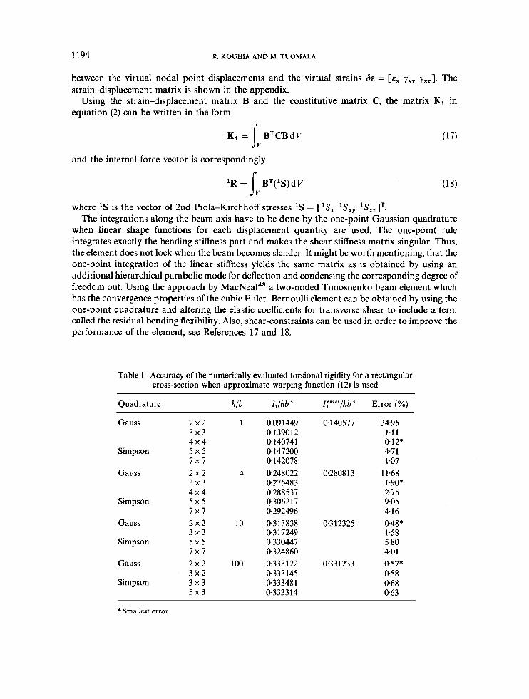
when linear shape functions for each displacement quantity are used. The one-point rule integrates exactly the bending stiffness part and makes the shear stiffness matrix singular. Thus, the element does not lock when the beam becomes slender. It might be worth mentioning, that the one-point integration of the linear stiffness yields the same matrix as is obtained by using an additional hierarchical parabolic mode for deflection and condensing the corresponding degree of freedom out. Using the approach by MacNea14' a two-noded Timoshenko beam element which has the convergence properties of the cubic Euler-Bernoulli element can be obtained by using the one-point quadrature and altering the elastic coefficients for transverse shear to include a term called the residual bending flexibility. Also, shear-constraints can be used in order to improve the performance of the element, see References 17 and 18.
Table I. Accuracy of the numerically evaluated torsional rigidity for a rectangular cross-section when approximate warping function (12) is used
Quadrature hlb I,/hb3 I Y ' / h b 3 Error (%)
Gauss
Simps o n
Gauss
Simpson
Gauss
Simpson
Gauss
Simpson
2 x 2 1 3 x 3 4 x 4 5 x 5 7 x 7 2 x 2 4 3 x 3 4 x 4 5 x 5 7 x 7 2 x 2 10 3 x 3 5 x 5 7 x 7 2 x 2 100 3-x 2 3 x 3 5 x 3
Also, higher-order interpolation can be used yielding a subparametric element. However, in geometrically and materially non-linear analysis a computationally effective but simple beam element can be obtained by using a linear interpolation for ge~metry.~’
Over the cross-sectional area either Gauss or Simpson integration rules can be used. In the elastic case and when the cross-section is narrow (h/b 3 10) the 2 x 2 Gaussian or the 3 x 3 Simpson rule is sufficient, although these rules underintegrate the torsional constant term
4 = lA “Y - %)’ + (2 + @ , Y ) ’ l d’4 (19)
when the approximate warping function (12) is used. However, the underintegrated torsional constant is closer to the exact value than the one obtained by using the 4 x 4 Gaussian rule, which integrates expression (19) exactly. When the cross-section is a square the 4 x 4 Gaussian rule gives the best accuracy, see Table I.
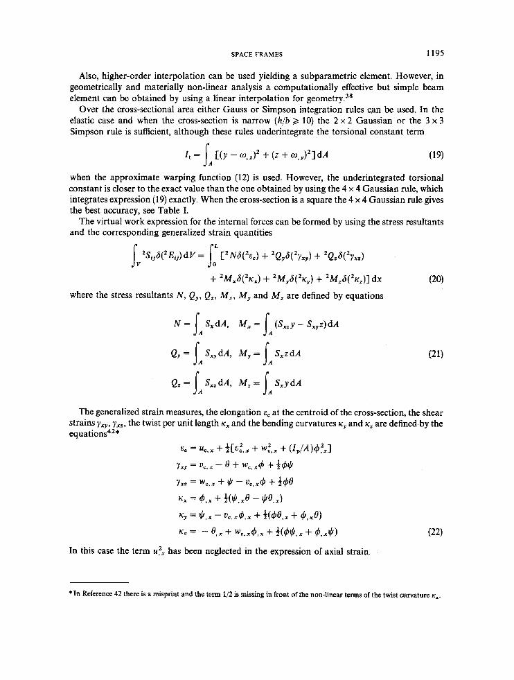
The virtual work expression for the internal forces can be formed by using the stress resultants and the corresponding generalized strain quantities
+ ’ M , ~ ( ’ K ~ ) + ’MY6(%,) + 2 M , S ( z ~ , ) ] dx where the stress resultants N , Q y , Q,, M,, M y and M , are defined by equations
N = [A &dA, Mx = lA ( L Y - Sxyz)dA
Q, = S,dA, M y = l A
The generalized strain measures, the elongation E, at the centroid of the cross-section, the shear strains y x y , y,,, the twist per unit length K , and the bending curvatures xy and K , are defined by the equations42*
Ec = %,x + m , x + w:,x + UP/44?J Y x y = %,X - 8 + wc, ,4 + a+* Y x z = we,, + * - % x 4 + 390 K x = 4 , x + W , x e - W , x )
KY = $,x - % x 4 , x + +(4& + 4 , A Kz = - 0.1 + WCJ4,X + % W , x + 4 , A )
In this case the term ufx has been neglected in the expression of axial strain.
*In Reference 42 there is a misprint and the term 1/2 is missing in front of the. non-linear terms of the twist curvature K ~ .
1196 R. KOUHIA AND M. TUOMALA
The vectors of stress resultants and generalized strains denoted by Z and e, respectively, are
= CN Q, Q, M x M y M,IT
e = C E C Y x y Yxz xx K , K,IT (23)
The constitutive law in the elastic case can be written in an incremental form
AX = CAe (24)
where C = diag[EA GAS, G A , GI , EI, E I , ]
in which EA is the axial rigidity, GAS, and GAS, are the shear stiffnesses in the y- and z-directions, respectively, GI, is the torsional rigidity and EI,, EI , are the bending stiffnesses about the y- and z-axes, respectively.
The internal force vector is calculated using the formula
'R = f: (BT)('Z)dx
The geometric stiffness matrix has a little simpler form than in the fully numerically integrated element, for details see Reference 42. The internal force vector, the geometric stiffness and the linear stiffness matrix
K, = {: BTCBdx
can now be integrated with respect to the axial co-ordinate only. This approach results in a simple way to formulate the finite element equations for a three-dimensional (3-D) beam. It is computa- tionally much more economical than the corresponding fully numerically integrated element. However, non-linear material behaviour cannot be modelled as accurately as in the layered model. For example, in the elastoplastic case the yield surface formulated using the stress resultants is quite complicated for general cross-sectional shapes. Therefore, simple approximate yield surfaces, expressed in terms of stress resultants, have usually been adopted in the analyses. However, the results of this kind of computation have to be interpreted with great care; see, for instance, the examples in Reference 40.
4. THIN-WALLED BEAMS
4.1. Kinematical relations of the warping displacement
The geometrically linear kinematical behaviour of a beam with a thin-walled open cross- section can be described based on the assumption that the projection of the cross-section on a plane normal to the centroidal axis does not distort during deformation, i.e. the cross-section is rigid in its projection plane. According to this assumption, the in-plane displacements of an arbitrary point of the cross-section undergoing a small twisting rotation can be expressed by three parameters: the two displacement components v, w and the angle of twist C$ about the longitudinal beam axis, i.e.
u = v, - zr#J
w = wc + yC$ (28)
SPACE FRAMES 1197
Because of material non-linearity, the shear centre location is not known in advance. Therefore, the displacement quantities are referred to an arbitrary point of the cross-section.
The axial displacement can be expressed in the form3', 40
u = u , - y y e + z J / - u s 9 - u r + , , (29) where u, is an arbitrary function depending only on the x-co-ordinate, w, is the warping function at the middle line of the cross-section of the beam and u, is the warping function due to the slab action
u,(s) = h,ds, o,(s, r) = hr(s)r (30) l: where
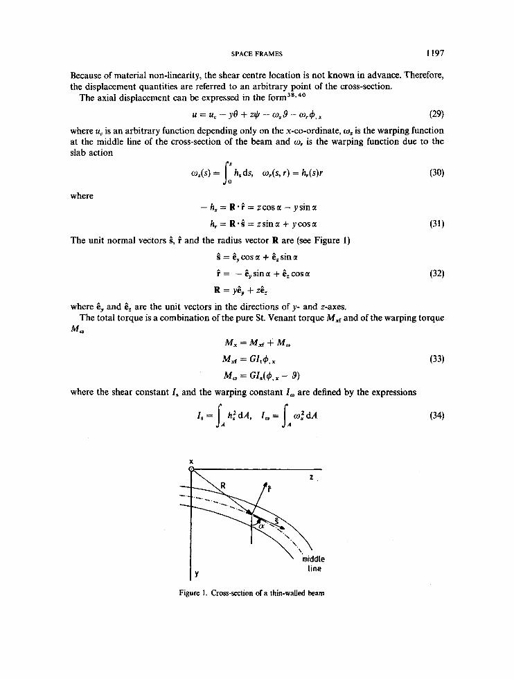
- h, = R - i = zcosa - ysina
h, = R - 3 = zsina + ycosa (31) The unit normal vectors k, i and the radius vector R are (see Figure 1)
3 = 6,cosa + 6,sina
i = - Cysina + &,cosa (32) R = $,, + 26,
where &y and GZ are the unit vectors in the directions of y- and z-axes.
M m The total torque is a combination of the pure St. Venant torque M d and of the warping torque
M x = Mxf + M ,
where the shear constant Is and the warping constant I, are defined by the expressions
X
line
Figure 1. Cross-section of a thin-walled beam
Y
(34)
1198 R. KOUHIA AND M. TUOMALA
The bimoment B is defined by the formula
B = - EI,$, , (35)
4.2. Thin-walled beam element
For a straight beam element with a thin-walled open cross-section, the displacement expres- sions are almost identical to those used for a beam with a solid cross-section. The only difference is that the warping displacement is divided into two parts:
u = u, - (6 - 449)Y + (9 + b # a z - w 4 , x - WS9, (36)
The axial variation of warping is independently interpolated within an element by the shape functions
9 = Nsq, (37)
A thin-walled beam element can also be formulated using the stress resultants and the corresponding generalized strain quantities. The internal virtual work expression for a thin- walled beam is
r f L
f 2 M , 6 ( 2 ~ , ) + 2 M , 6 ( 2 ~ , ) + 'BS('K,) + 2M,6(2y , ) ] dx (38)
The generalized strain measures ec , y x y , yxz, K,, K , and K , are defined in equations (22) and by the additional relations
Denoting the vector of stress resultants by E and the vector of generalized strains by e,
the elastic constitutive matrix can be written in the form of equation (24); see also Reference 76. An element based on Vlasov's classical theory of torsion concerning thin-walled member^,'^
can be simply constructed from the presented elements by using a penalty method. In an element, formulated by using the stress resultants and generalized strain quantities, the Vlasov constraint
can be taken into account by using a term aGI, instead of GI, in the constitutive matrix C, where a is a suitably chosen penalty parameter (u $. 1). In the other elements, the constraint (41) can be included by adding a term
to the variational equations.
5. TRANSFORMATION BETWEEN LOCAL AND GLOBAL CO-ORDINATE SYSTEMS
The orientation of a beam in the global X, Y, 2 space is completely defined if the beam axis and two directions of the cross-section perpendicular to the beam axis are known. The orthonormal
SPACE FRAMES 1199
base vectors of the global co-ordinate system in the X , Y and 2 directions are denoted by el, c2, c, and the orthonormal base vectors of the initial local co-ordinate system x, y, z by g1, t2, t 3 .
The initial orientation matrix of a beam can now be defined by
Qi = roci (43)
YOij = COS(&, G j ) (44)
where the elements of the matrix To are the direction cosines
At some equilibrium configuration C1, reached after n + 1 steps, the rotation matrix Y,+ can be obtained from the rotation matrix at the previous equilibrium configuration C1 (at step n) by the formula
Y,+, = AYY, (45)
where the incremental rotation matrix AY is calculated from the incremental displacements between C1 and Cz.
The element stiffness matrix and the internal force vector, evaluated in the local co-ordinate system, are transformed to the global co-ordinate system in a well-known manner, see References 7 and 10.
Connections of the thin-walled beam elements in a general 3-D assemblage present difficulties. At the present stage, in the computer code developed, free or full warping restraint can be modelled. In practice, therc are many different ways to connect thin-walled members, and the accurate modelling of connections in each case needs further study. A universal solution for completely general cross-section shapes may not be possible, as pointed out in References 45 and 46.
6. CONSTITUTIVE MODELS
6. I. Layered approach
Incremental constitutive equations suitable for computational purposes can be based on a rate-type plasticity theory by Hill.33 The strain rate 9 is decomposed into elastic, plastic and thermal parts
9 = g e + 9 p + @ (46)
9 0 = @&% (47)
The J2-flow theory is used to evaluate the plastic strain rate and the thermal strain rate is
where E is the coefficient of thermal expansion which is assumed to be constant and 9 is the unit tensor.
The elastic part 23e is related to the co-rotational Zaremba-Jaumann rate of Cauchy stress tensor F by a linear law
(48) * y = Ve :9 " = Ve:(9 - P),
in which V" is the elastic constitutive tensor. In the J2-flow theory, the yield function is
f = J 3 ~ 2 - o,(k, 0) (49) where the yield stress oy depends on a hardening parameter k and temperature 8 and J 2 is the second invariant of the deviatoric Cauchy stress tensor. The plastic part of the strain rate is
1200 R. KOUHlA A N D M. TUOMALA
obtained from a plastic potential by using a normality law and a consistency condition of plastic
For rate-dependent material behaviour the strain rate is decomposed into elastic and viscop- flow.33.34
lastic parts. Perzyna6' has given the following expression for the viscoplastic part
where f = &, y is the viscosity coefficient, oy the static yield limit and p is a material parameter. The notation ( x } has the meaning
0 i fx ,<O x i f x > O (x> =
6.2. Yield surfaces expressed in terms of stress resultants
Denoting the vector of stress resultants by E, the yield function can be expressed in the form
f (El = 0 (52) For a 3-D beam with an arbitrary cross-sectional shape the function f would be very complex. Yang et ~ 1 . ~ ~ have discussed the form of the yield surface for a doubly symmetric I-section under five active forces N, M,, M y , M, and B. However, in analysing the response under strong transient loadings, the effect of shear forces becomes important and cannot be neglected in the yield function expression. Simo et ~ 1 . ~ ~ have proposed a stress resultant yield function for a plane Timoshenko beam containing the shear force. In this study two simple approximate yield functions have been used. The first, a hypersphere, has the form (z),' = i
i = 1
where n, is the number of stress resultants. The second one, a hypercube yield surface, is
(53)
In equations (53) and (54), Zpi is the fully plastic value of the corresponding stress resultant.
7. NUMERICAL EXAMPLES
The discretized equilibrium equations are solved by using a variant of the arc-length continuation procedure6', 16, 63, 29 which is described in more detail in References 40 and 39. Integration of the equations of motion has been done by using the central difference method or by the midpoint version of the trapezoidal 51
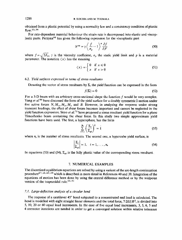
7.1. Large-defection analysis of a circular bend
The response of a cantilever 45" bend subjected to a concentrated end load is calculated. The bend is modelled with eight straight linear elements and the total force, 7-2EI/R2, is divided into 5, 10, 20 or 60 equal load increments. In the case of five equal load increments, 3, 5, 6, 5 and 4 corrector iterations are needed in order to get a converged solution within relative tolerance
SPACE FRAMES 1201
of linearization is studied. The results of computations when the approximation
with respect to the weighted displacement riter ria.^' Also the effect of using inconsistent
E Z I + G ?
is used for the rotation matrix (8) are shown in Table 11. In this particular example the errors due to the inconsistency are not so striking than in the examples presented in Reference 42. The
Table 11. Comparison of tip deflections of a circular bend
NEL* Shape function NINC’ - u / R - u / R w/R
E % I + Q 8 Linear 10 0-135 0-231 0.533 E % I + S l 8 Linear 20 0.137 0.230 0.533 E % : r + Q 8 Linear 60 0137 0229 0.532 B % I + Q +in’ 8 Linear 5 0136 0238 0537 I % I + n + i n 2 8 Linear 10 0.136 0.238 0.535 S % : r + Q + in’ 8 Linear 20 0.136 0.237 0,535 B % I + n + in’ 8 Linear 60 0.136 0.237 0.535 Bathe and Bolourchi’ 8 Cubic 60 0.134 0.235 0.534 Simo and VU-QUOC’~ 8 Linear 3 0-135 0-235 0.534 Cardona and GeradinL4 8 Linear 6 0.138 0.237 0535 Dvorkin et ~ 1 . ’ ~ 5 Parabolic 10 0.136 0.235 0.533 Surana and S ~ r e r n ’ ~ 8 Parabolic 7 0.133 0.230 0.530 Crisfield” 8 Cubic 3 0.137 0.239 0.537 Sandhu et ~ 1 . ~ ’ 8 Linear 3 0.134 0.234 0.533
* Number of elements Number of load steps
0.0 0.1 0.2 0.3 0.4 0.5 0.6 non-dimensional tip deflection
Figure 2. Large-deflection analysis of a 45“ circular bend
1202 R. KOUHIA AND M. TUOMALA
pure-load-controlled Newton method is used to solve the non-linear equations of equilibrium. The load-tip-deflection curves are shown in Figure 2, when 20 equal load increments are used. In the same figure also the results from a calculation with eight beam-column elements by Virtanen and M i k k ~ l a , ~ ~ are presented. They agree well with the present results. The calculated tip deflections are compared with those reported by Bathe and Bol~urchi ,~ Simo and VU-QUOC,’~ Dvorkin et u Z . , ’ ~ Surana and S ~ r e m , ~ ’ Crisfield” and Sandhu et in Table 11. The differences between various algorithms are small and it may be concluded that this particular example is not a serious test case for procedures handling large rotation effects.
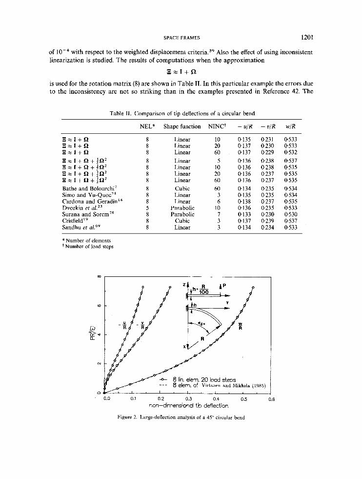
7.2. Instability analysis of a framed dome
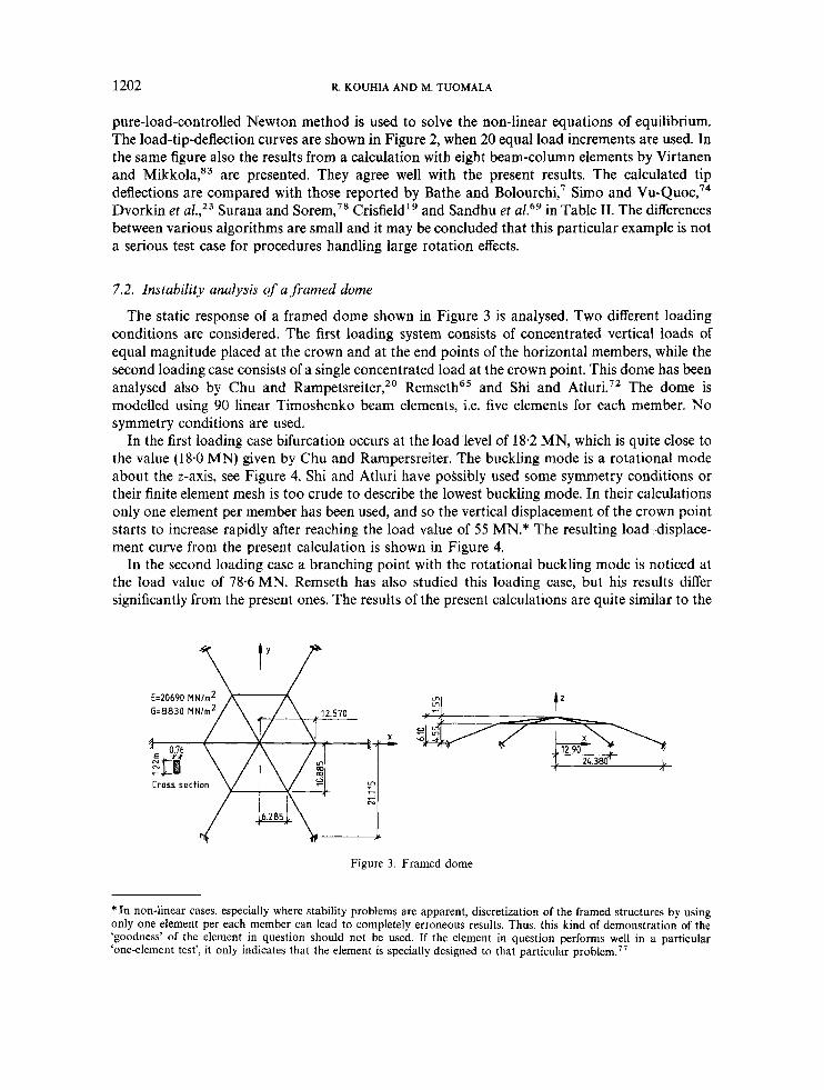
The static response of a framed dome shown in Figure 3 is analysed. Two different loading conditions are considered. The first loading system consists of concentrated vertical loads of equal magnitude placed at the crown and at the end points of the horizontal members, while the second loading case consists of a single concentrated load at the crown point. This dome has been analysed also by Chu and Rampetsreiter,’* R e m ~ e t h ~ ~ and Shi and A t l ~ r i . ~ ~ The dome is modelled using 90 linear Timoshenko beam elements, i.e. five elements for each member. No symmetry conditions are used.
In the first loading case bifurcation occurs at the load level of 18-2 MN, which is quite close to the value (18-0 MN) given by Chu and Rampersreiter. The buckling mode is a rotational mode about the z-axis, see Figure 4. Shi and Atluri have possibly used some symmetry conditions or their finite element mesh is too crude to describe the lowest buckling mode. In their calculations only one element per member has been used, and so the vertical displacement of the crown point starts to increase rapidly after reaching the load value of 55 MN.* The resulting load-displace- ment curve from the present calculation is shown in Figure 4.
In the second loading case a branching point with the rotational buckling mode is noticed at the load value of 78.6 MN. Remseth has also studied this loading case, but his results differ significantly from the present ones. The results of the present calculations are quite similar to the
Crass section
Figure 3. Framed dome
*In non-linear cases, especially where stability problems are apparent, discretization of the framed structures by using only one element per each member can lead to completely erroneous results. Thus, this kind of demonstration of the ‘goodness’ of the element in question should not be used. If the element in question performs well in a particular ‘one-clement test’, it only indicates that the element is specially designed to that particular problem.”
SPACE FRAMES 1203
0 2 4 6 8 1 0
w / m
Figure 4. Framed dome, vertical displacement of the apex vs. load and the rotational buckling mode
0 0
0 m
g g \
0 0 2 4 6 8
w / m Figure 5. Load-displacement curve of a framed dome when a concentrated load alone acts at the crown point
results obtained by Shi and Atluri. However, they have not noticed the bifurcation point. The load-deflection curve from the unstable symmetric deformation mode is drawn with dashed line in Figure 5. The results from the computation of the symmetric deformation mode are in good agreement with the results by Shi and Atluri.
7.3. Elastoplastic lateral buckling analysis of simply supported I-beams
Kitipornchai and Trahair36 have made an experimental investigation of the inelastic flexural-torsional buckling of rolled steel I-beams. Their tests were carried out on full-scale simply supported 261 x 151 UB 43 beams with central concentrated loads applied with a gravity load simulator. The 261 x 151 UB 43 section has a low width to thickness ratio of the flanges and so the beam behaviour inhibits local buckling and allows lateral buckling to predominate. The end cross-sections of each beam were free to rotate about the major and minor axes and to warp. They tested six beams, four as-rolled and two annealed beams. The effect of residual stresses was
1204 R. KOUHIA AND M. TUOMALA
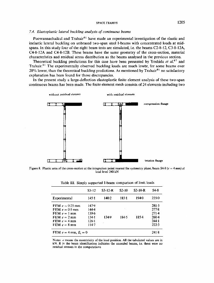
not found to be significant which was also confirmed by the theoretical predictions made by Kitipornchai and Trahair3' and by the numerical computations in the present study. The reason is in high tensile residual stresses which inhibit the spread of plasticity in the compression flange; see Figure 8. The geometrical imperfections were found to be significant in decreasing the load-carrying capacity.
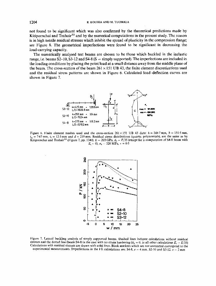
The numerically analysed test beams are chosen to be those which buckled in the inelastic range, i.e. beams S2-10, S3-12 and S4-8 (S = simply supported). The imperfections are included in the loading conditions by placing the point load at a small distance away from the middle plane of the beam. The cross-section of the beam 261 x 151 UB 43, the finite element discretizations used and the residual stress patterns are shown in Figure 6. Calculated loaddeflection curves are shown in Figure 7.
Figure 6. Finite element meshes used and the cross-section 261 x 151 UB 43 data: h = 248.7 mm, b = 151.5 mm, tw = 7.67 mm, tc = 12.3 mm and d = 219 mm. Residual stress distributions (quartic polynomials), are the same as by Kitipornchai and Trahair3s (Figure 7, pp. 1340). E = 203 GPa, Et = E/35 (except for a computation of 54-8 beam with
Et = 0), oY = 320 MPa, v = 0.3
0 I D - N
0 0 - N
0
5 s L O -
-
\ -
sz
0 -6 0 6 10 16 20 26
w / m m
Figure 7. Lateral buckling analysis of simply supported beams. Dashed lines indicate calculations without residual stresses and the dotted line (beam 54-8) is the case with no strain hardening (E, = 0, in all other calculations E, = E/35) Calculations with residual stresses are drawn with solid lines. Black markers which are not connected correspond to the
experimental measurements. Imperfections in the FE calculations are: S4-8, e = 4 mm, S2-10 and S3-12, e = 2 mm
SPACE FRAMES 1205
7.4. Elastoplastic lateral buckling analysis of continuous beams
Poowannachaikul and Trahair6' have made an experimental investigation of the elastic and inelastic lateral buckling on unbraced two-span steel I-beams with concentrated loads at mid- spans. In this study four of the eight beam tests are simulated, i.e. the beams C2-8-12, C3-8-12A, C4-8-12A and C4-8-12B. These beams have the same geometry of the cross-section, material characteristics and residual stress distribution as the beams analysed in the previous section.
Theoretical buckling predictions for this case have been presented by Yoshida et aL8' and Trahair.81 The experimentally observed buckling loads are much lower, for some beams over 20% lower, than the theoretical buckling predictions. As mentioned by Trahair*' no satisfactory explanation has been found for those discrepancies.
In the present study a large-deflection elastoplastic finite element analysis of these two-span continuous beams has been made. The finite element mesh consists of 24 elements including two
without residual stresses with residual stresses
compression flange
tension flange
Figure 8. Plastic area of the cross-section at the integration point nearest the symmetry plane, beam S4-8 (e = 4 mm) at load level 240 kN
Table 111. Simply supported I-beam: comparison of limit loads
S3-12 S3-12-R S2-10 S2-10-R S4-8
Experimental 145.1 1402 185.1 194.0 235.0
FEM e = 0.25 mm 147.9 281.3 FEM e = 0.5 mm 144.4 277.8 FEM e = 1 mm 139.6 271.4 FEM e = 2mm 134.1 134.9 184.5 185.4 260.4 FEM e = 4mm 126.1 244.1 FEM e = 8 mm 114.7 222.3
FEMe=4mm,E,=O 241-8
Notes: e means the eccentricity of the load position. All the tabulated values are in kN. R in the beam identification indicates the annealed beams, i.e. there were no residual stresses in the computations
1206 R. KOUHIA AND M. TUOMALA
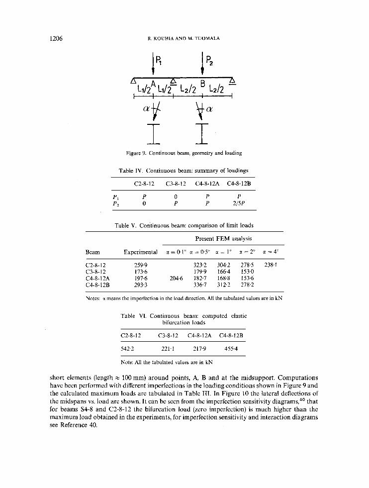
I I Figure 9. Continuous beam, geometry and loading
Table 1V. Continuous beam: summary of loadings
C2-8-12 C3-8-12 C4-8-12A C4-8-12B
p , P 0 P P p2 0 P P 215 P
Table V. Continuous beam: comparison of limit loads
Present FEM analysis
Beam Experimental 0: = 0.1" a = 0.5" a = 1" z = 2" LY = 4"
Notes: CL means the imperfection in the load direction. All the tabulated values are in kN
Table VI. Continuous beam: computed elastic bifurcation loads
C2-8-12 C3-8-12 C4-8-12A C4-8-12B
542.2 221.1 217.9 455.4
Note: All the tabulated values are in kN
short elements (length zz 100 mm) around points, A, B and at the midsupport. Computations have been performed with different imperfections in the loading conditions shown in Figure 9 and the calculated maximum loads are tabulated in Table 111. In Figure 10 the lateral deflections of the midspans vs. load are shown. It can be seen from the imperfection sensitivity diagram^,^' that for beams 54-8 and C2-8-12 the bifurcation load (zero imperfection) is much higher than the maximum load obtained in the experiments, for imperfection sensitivity and interaction diagrams see Reference 40.
SPACE FRAMES 1207
z
e
Y \
0 0 0
0 0 cu
0 E
0 -16 -10 -5 0 5 10 15
w / m m
0 0 0
z8 Ycu \
e 0 9
0 -16 -10 -6 0 6 10 16
w / m m
z
e
Y \
0 0 N
0 2
0 -16 -10 -6 0 6 10 16
w / m m
0 0 m
C4-8-12A
2 8 Ycu \ e
0 2
0 ' ' I ' ' ' " I I ' I
-16 -10 -6 0 6 10 16 w / m m
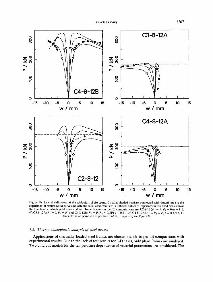
Figure 10. Lateral deflections at the midpoints of the spans. Circular shaded markers connected with dotted line are the experimental results. Solid curves indicate the calculated results with different values of imperfection. Blanked circles show the load level at which yield is noticed first. Imperfections in the FE computations are: C2-8-12 (P1 = P, P2 = 0) a = 1,2, 4'; C3-8-12A ( P , = 0, P z = P) and C4-8-12B (P1 = P, P2 = 2/5P) a = 0.5,1,2", C4-8-12A ( P , = P, = P ) E = 0.1,0.5, 1".
Deflections at point A are positive and at B negative; see Figure 9
Applications of thermally loaded steel frames are chosen mainly to permit comparisons with experimental results. Due to the lack of test results for 3-D cases, only plane frames are analysed. Two different models for the temperature dependence of material parameters are considered. The
1208 R. KOUHIA AND M. TUOMALA
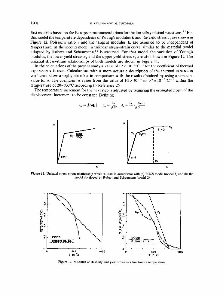
first model is based on the European recommendations for the fire safety of steel structure^.^' For this model the temperature dependence of Young’s modulus E and the yield stress oy are shown in Figure 12. Poisson’s ratio v and the tangent modulus E, are assumed to be independent of temperature. In the second model, a trilinear stress-strain curve, similar to the material model adopted by Rubert and Schaumann,68 is assumed. For that model the variation of Young’s modulus, the lower yield stress op and the upper yield stress oy are also shown in Figure 12. The uniaxial stress-strain relationships of both models are shown in Figure 1 1 .
In the calculations of the present study a value of 12 x 10-60C-’ for the coefficient of thermal expansion a is used. Calculations with a more accurate description of the thermal expansion coefficient show a negligible effect in comparison with the results obtained by using a constant value for CI. The coefficient a varies from the value of 1 . 2 ~ to 1 . 7 ~ 10-50C-1 within the temperature of 20-600°C according to Reference 25.
The temperature increment for the next step is adjusted by requiring the estimated norm of the displacement increment to be constant. Defining
U
E
u
f I - 0 y I I
EfTi I ; 1%
E
Figure 11. Uniaxial stress-strain relationship which is used in accordance with (a) ECCS model (model 1) and (b) the model developed by Rubert and Schaumann (model 2)
0 so0 1000 0 so0 1000 T In *C T In *C
Figure 12. Modulus of elasticity and yield stress as a function of temperature
SPACE FRAMES 1209
where A# is the temperature increment, the requirement for the next step is
un+l = v , A B , + ~ + ia,(Ae,+1)2 = u,
which yields
If a, = 0, then the equality A&+ = A#, holds. However, in numerical computations the temper- ature increment for the next step is determined from the approximate expression
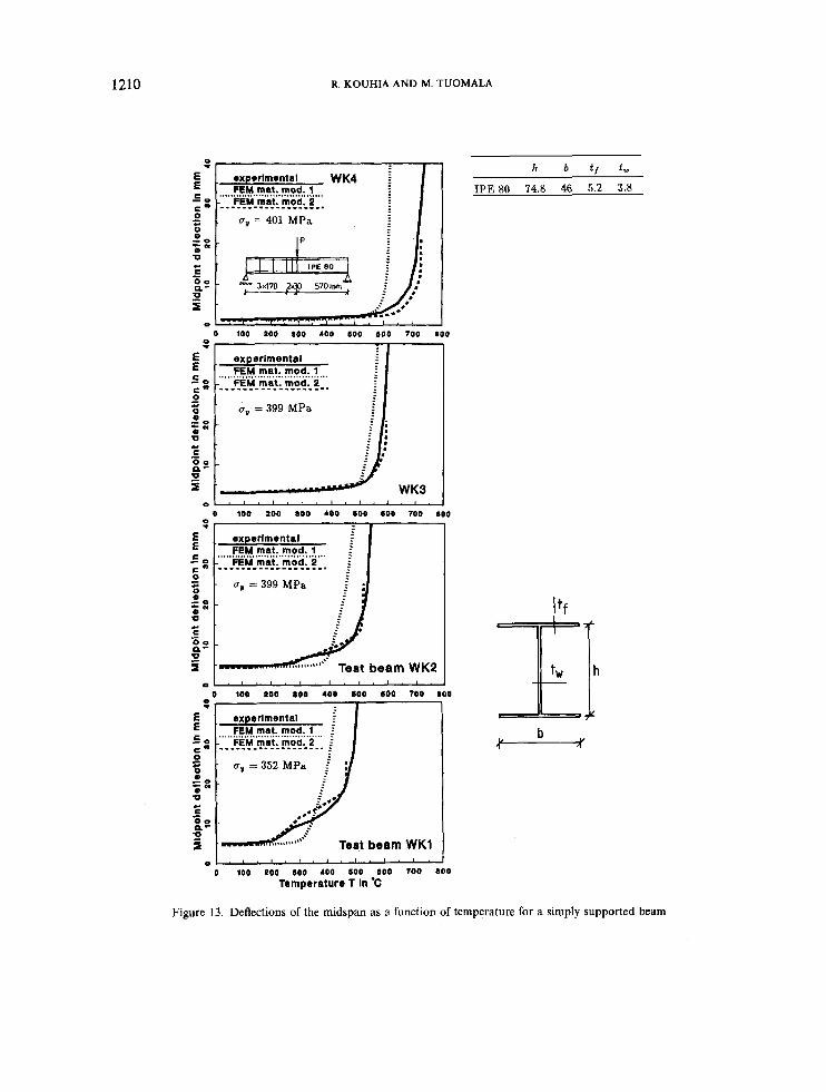
Rubert and Schaumann have made experimental and computational analyses of simply supported IPE-80 beams with a concentrated load at the midspan. Four different load mag- nitudes are used, P = 24, 23, 16 and 6 kN for beams WK1-4. The corresponding utilization factors are P/P, = 0.85, 0.70, 0.50, 0.20, respectively. The present results of quasi-static calcu- lations are compared with the experimental results, where the lowest value of the heating rate 6 = 2.67 K/min is used. According to the experimental results the effect of heating rate, which varied in the range 2-67-32 K/min in the experiments, is not significant to the behaviour of the beams WK1 and WK2. For the beam WK4, which has the lowest load, the effect of heating rate results in 10 per cent difference in the critical temperature. One-half of the beam is modelled with five linear elements using two short elements near the symmetry line. The initial temperature increment used is 20°C and it was automatically reduced during the heating process according to equation (55).
The results of the computations where the material parameters of the second model are used agree very well with the experimental results in this particular example. Especially, the influence of the slow decrease interval of the lower yield stress between 300 and 500°C is clearly seen in the deflection-temperature curves for beams WK1 and WK2, see Figure 13. This slow increase interval of the displacement has also been noticed in the calculations made by Rubert and Schaumann but it is not visible in the results obtained by Bock and Werner~son '~ in their calculations using the ADINA program. More examples are presented in References 37 and 40.
7.6. Dynamic plastic bifurcation of a pin-ended beam
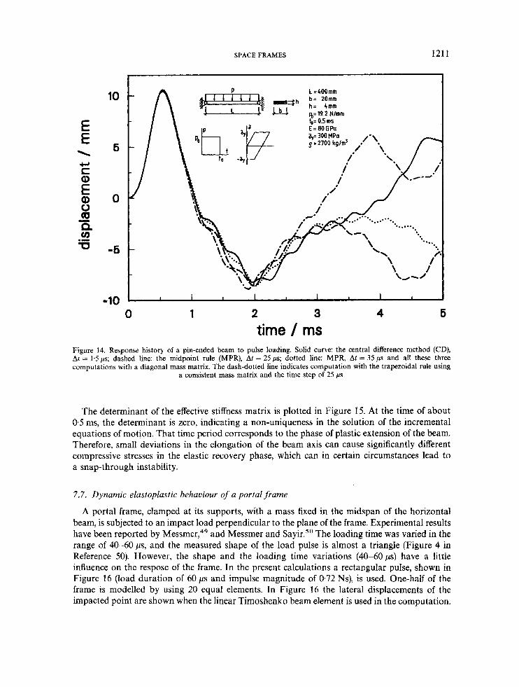
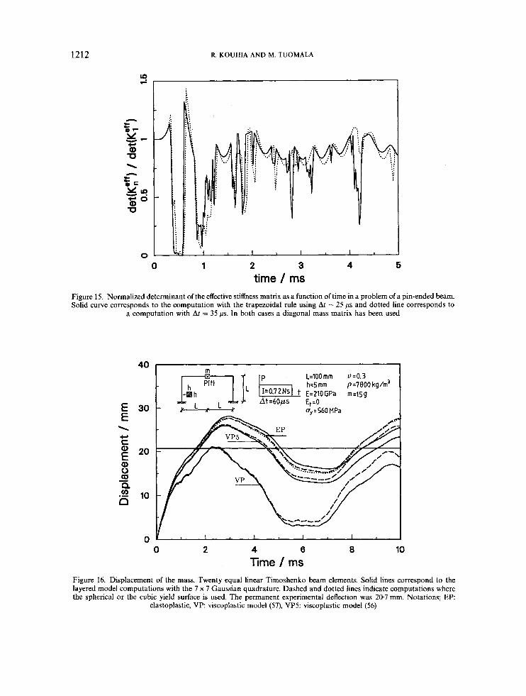
The behaviour of a pin-ended beam subjected to a uniform transverse loading applied as a short pulse is studied. The deflection history depends, in an extremely sensitive manner, on the interplay between momentum transfer, geometry changes and energy dissipation in plastic flow as pointed out by Symonds et d . * O Symonds and Yu79 give results of computations using ten different FE codes. An agreement in the prediction of the first peak deflection by all the different codes is obtained but the permanent displacements differ significantly. The unexpected result of those computations was the negative permanent displacement, implying that the final rest displacement is in the opposite direction to that of the load.
In the present analysis one-half of the beam is modelled by ten linear Timoshenko beam elements. The central difference scheme with a diagonal mass matrix and the time step of 1.5 ps gives a permanent deflection in the direction of the load. Also the midpoint rule with the time step of 25 ,us and a consistent mass matrix yields qualitatively the same result, but the time vs. midpoint deflection curve starts to differ significantly after 1 ms. When the midpoint rule with a diagonal mass matrix and the time steps of 25 and 35 p s are used, negative permanent deflections occur. These four completely different deflection histories are shown in Figure 14.
1210 R. KOUHIA AND M. TUOMALA
0
0
E E
o too POD aoo 400 600 600 TOO BOO
experimental FEM mat. mod. 1 .....................................
- FEM mat. mod. 2-. ---------.-----.. ' by = 399 MPa
- - : a : . : I : . : .
WK3
B " " " " " " " '
0 100 SO0 800 400 600 600 TOO 100 0
I I E E FEM mat. mod. 1 .....................................
- FEM mat. mod. 2
Test beam WK1
IPE 80 74.8 46 5.2 3.8
c " " " " " ' 1 o loo POO aoo 400 600 eoo TOO LOO
Temperature T In 'C
Figure 13. Deflections of the midspan as a function of temperature for a simply supported beam
SPACE FRAMES 1211
10
6
0
P 1 =4OOmm i l l 1 1 -sh b = 20mm ’u‘ lihJ. h- ~=19.2Nlrnm 4mm
L= 0.5 ns
-10 ’ I I I I I I I I I
0 1 2 3 4 5 time 1 ms
Figure 14. Response history of a pin-ended beam to pulse loading. Solid curve: the central difference method (CD), At = 1.5 p; dashed line: the midpoint rule (MPR), At = 25 p; dotted line: MPR, At = 35 p s and all these three computations with a diagonal mass matrix. The dash-dotted line indicates computation with the trapezoidal rule using
a consistent mass matrix and the time step of 25 ps
The determinant of the effective stiffness matrix is plotted in Figure 15. At the time of about 0.5 ms, the determinant is zero, indicating a non-uniqueness in the solution of the incremental equations of motion. That time period corresponds to the phase of plastic extension of the beam. Therefore, small deviations in the elongation of the beam axis can cause significantly different compressive stresses in the elastic recovery phase, which can in certain circumstances lead to a snap-through instability.
7.7. Dynamic elastoplastic hehauiour of a portal frame
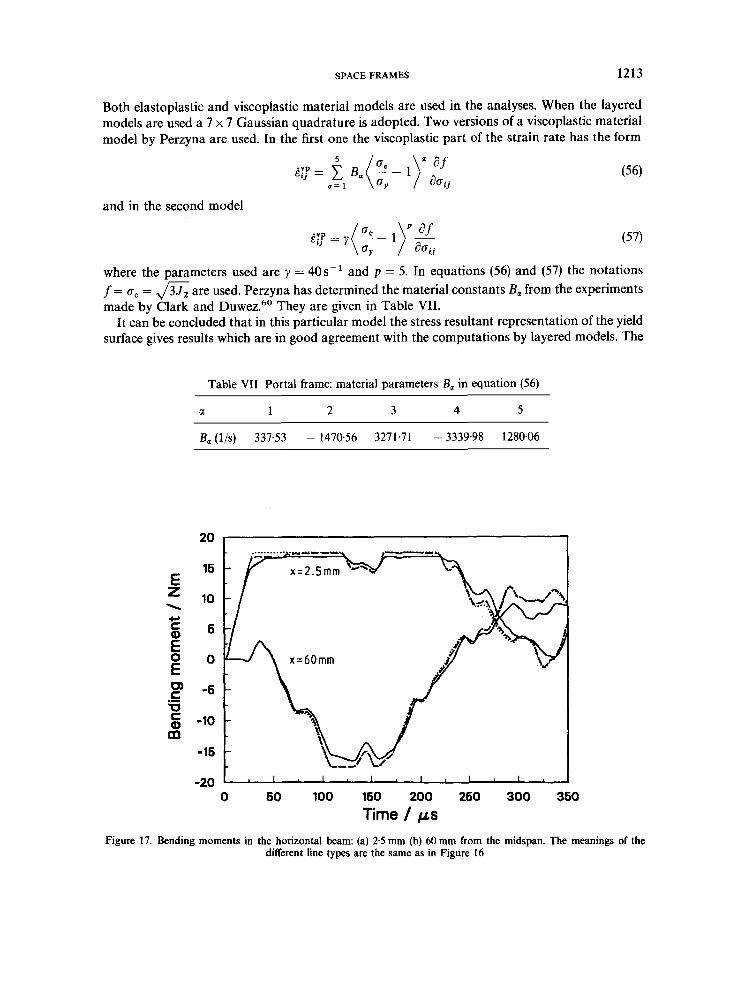
A portal frame, clamped at its supports, with a mass fixed in the midspan of the horizontal beam, is subjected to an impact load perpendicular to the plane of the frame. Experimental results have been reported by Me~smer:~ and Messmer and Sayir.” The loading time was varied in the range of 40-60 ps, and the measured shape of the load pulse is almost a triangle (Figure 4 in Reference 50). However, the shape and the loading time variations (40-60 ,us) have a little influence on the respose of the frame. In the present calculations a rectangular pulse, shown in Figure 16 (load duration of 60 p s and impulse magnitude of 0.72 Ns), is used. One-half of the frame is modelled by using 20 equal elements. In Figure 16 the lateral displacements of the impacted point are shown when the linear Timoshenko beam element is used in the computation.
1212 R. KOUHIA A N D M. TUOMALA
rq
n
0 -
u- c,
c c
Y a U \ n t m c
CrO a U
g s
0 0 1 2 3 4 6
time / ms Figure 15. Normalized determinant of the effective stiffness matrix as a function of time in a problem of a pin-ended beam. Solid curve corresponds to the computation with the trapezoidal rule using At = 25 p s and dotted line corresponds to
a computation with At = 35 p. In both cases a diagonal mass matrix has been used
40
E 30
; 20 \
c c,
a 0 (0
0. -
10 6
0 0 2 4 6 8 10
Time / ms Figure 16. hplacement of the mass. Twenty equal linear Timoshenko beam elements. Solid lines correspond to the layered model computations with the 7 x 7 Gaussian quadrature. Dashed and dotted lines indicate computations where the spherical or the cubic yield surface is used. The permanent experimental deflection was 20.7 mm. Notations; E P
elastoplastic, V P viscoplastic model (57), VYS: viscoplastic model (56)
SPACE FRAMES 1213
Both elastoplastic and viscoplastic material models are used in the analyses. When the layered models are used a 7 x 7 Gaussian quadrature is adopted. Two versions of a viscoplastic material model by Perzyna are used. In the first one the viscoplastic part of the strain rate has the form
and in the second model
where the parameters used are y = 40s-1 and p = 5. In equations (56) and (57) the notations f = ae = & are used. Perzyna has determined the material constants B, from the experiments made by Clark and Duwez.60 They are given in Table VII.
It can be concluded that in this particular model the stress resultant representation of the yield surface gives results which are in good agreement with the computations by layered models. The
Table VII Portal frame: material parameters B, in equation (56)
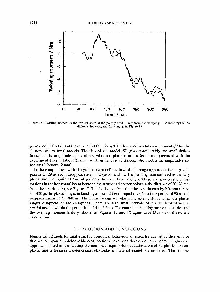
Figure 17. Bending moments in the horizontal beam: (a) 2 5 mm (b) 60 mm from the midspan. The meanings of the different line types are the same as in Figure 16
1214
2
0
-2
-4
-6
-8
R. KOUHIA AND M. TUOMALA
I
0 60 100 160 200 260 300 360 Time / ps
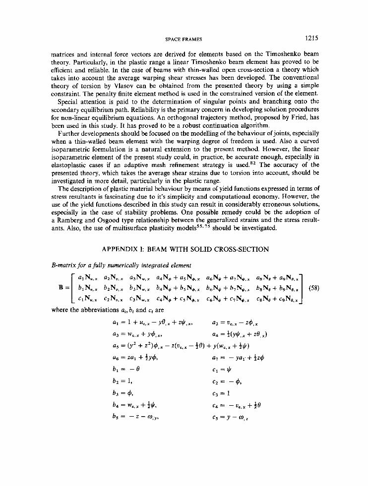
Figure 18. Twisting moment in the vertical beam at the point placed 20 mm from the clampings. The meanings of the different line types are the same as in Figure 16
permanent deflections of the mass point fit quite well to the experimental measurement^,^^ for the elastoplastic material models. The viscoplastic model (57) gives considerably too small deflec- tions, but the amplitude of the elastic vibration phase is in a satisfactory agreement with the experimental result (about 21 mm), while in the case of elastoplastic models the amplitudes are too small (about 12 mm).
In the computation with the yield surface (54) the first plastic hinge appears at the impacted point after 29 p s and it disappears at t = 120 p s for a while. The bending moment reaches the fully plastic moment again at t = 160 p s for a duration time of 60 ps . There are also plastic defor- mations in the horizontal beam between the struck and corner points in the distance of 50-80 mm from the struck point, see Figure 17. This is also confirmed in the experiments by M e ~ s m e r . ~ ~ At t = 420 ,us the plastic hinges in bending appear at the clamped ends for a time period of 90 p s and reappear again at t = 840 ps. The frame swings out elastically after 3.59 ms when the plastic hinges disappear at the clampings. There are also small periods of plastic deformation at t = 5.6 ms and within the period from 6-4 to 6-8 ms. The computed bending moment histories and the twisting moment history, shown in Figures 17 and 18 agree with Messmer’s theoretical calculations.
8. DISCUSSION AND CONCLUSIONS
Numerical methods for analysing the non-linear behaviour of space frames with either solid or thin-walled open non-deformable cross-sections have been developed. An updated Lagrangian approach is used in formulating the non-linear equilibrium equations. An elastoplastic, a visco- plastic and a temperature-dependent elastoplastic material model is considered. The stiffness
SPACE FRAMES 1215
matrices and internal force vectors are derived for elements based on the Timoshenko beam theory. Particularly, in the plastic range a linear Timoshenko beam element has proved to be efficient and reliable. In the case of beams with thin-walled open cross-section a theory which takes into account the average warping shear stresses has been developed. The conventional theory of torsion by Vlasov can be obtained from the presented theory by using a simple constraint. The penalty finite element method is used in the constrained version of the element.
Special attention is paid to the determination of singular points and branching onto the secondary equilibrium path. Reliability is the primary concern in developing solution procedures for non-linear equilibrium equations. An orthogonal trajectory method, proposed by Fried, has been used in this study. It has proved to be a robust continuation algorithm.
Further developments should be focused on the modelling of the behaviour of joints, especially when a thin-walled beam element with the warping degree of freedom is used. Also a curved isoparametric formulation is a natural extension to the present method. However, the linear isoparametric element of the present study could, in practice, be accurate enough, especially in elastoplastic cases if an adaptive mesh refinement strategy is used.82 The accuracy of the presented theory, which takes the average shear strains due to torsion into account, should be investigated in more detail, particularly in the plastic range.
The description of plastic material behaviour by means of yield functions expressed in terms of stress resultants is fascinating due to it’s simplicity and computational economy. However, the use of the yield functions described in this study can result in considerably erroneous solutions, especially in the case of stability problems. One possible remedy could be the adoption of a Ramberg and Osgood type relationship between the generalized strains and the stress result- ants. Also, the use of multisurface plasticity models5 5* 7 5 should be investigated.
APPENDIX I: BEAM WITH SOLID CROSS-SECTION
B-matrix for a fully numerically integrated element
where the abbreviations a i , bi and ci are
1216 R. KOUHIA AND M. TUOMALA
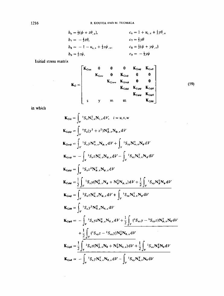
Initial stress matrix
in which
SPACE FRAMES 1217
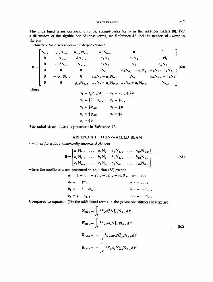
The underlined terms correspond to the second-order terms in the rotation matrix (8). For a discussion of the significance of these terms, see Reference 42 and the numerical examples therein.
B-matrix for a stress-resultant-based element
where
1 a5 = f*,,, a6 = 24 a7 = t d , x , as = $0
a9 = $* The initial stress matrix is presented in Reference 42.
APPENDIX 11: THIN-WALLED BEAM
B-matrix for a fully numerically integrated element
1 1 u,x . . . a4N+ + . . . aloN8,, I%= blN,,, . - . b4N, + b5N,. . . . btON$,x r N C I N ~ , ~ . . . c,N+ + C~N,,, . . . C ~ O N ~ , ~
where the coefficients are presented in equation (58) except al = 1 + uc, - ye, + z$, - w, 8, x, a7 = zal
a9 = -ya1, a10 = osa1
b5 = - z - o, ,~.
c5 = Y - a r , z c10 = - %,z
bl0 = - ws,y
Compared to equation (59) the additional terms in the geometric stiffness matrix are
KGLM = lSxwfNi.xN$,xdV I 6’
I V
KG198 = SxYoX, xN8, d V
KG+8= - lSxzosN~,,Ng,xdV
K G u 8 = - ISXw,N~,.NS,.dV
1218 R. KOUHIA AND M. TUOMALA
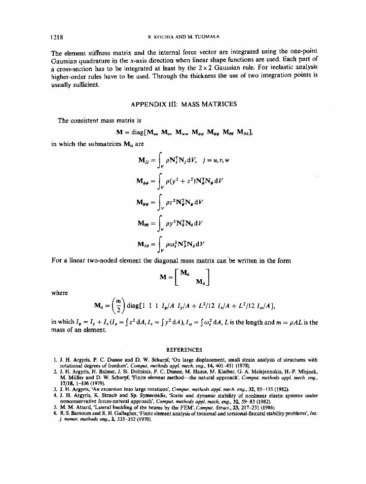
The element stiffness matrix and the internal force vector are integrated using the one-point Gaussian quadrature in the x-axis direction when linear shape functions are used. Each part of a cross-section has to be integrated at least by the 2 x 2 Gaussian rule. For inelastic analysis higher-order rules have to be used. Through the thickness the use of two integration points is usually sufficient.
APPENDIX 111: MASS MATRICES
The consistent mass matrix is
M = diagCMm M,, M,, Me, Me, MBB M d , in which the submatrices Mii are
M.. = pNFNjdV, j = u,u,w
M4+ = 1 p ( y 2 + z2)N:N4dV
& = Ivpz2N:N,dV
” b
1:
Y
Moo = py2N:NodV
MSS = Iy pwfNrNSdV
For a linear two-noded element the diagonal mass matrix can be written in the form
where
Md = - diag[l 1 1 I,/A I, /A + L2/12 [,/A + L2/12 I , /A] , (3 in which I, = I, + I , (I, = J z2 dA, I, = J y 2 dA), I, = 0: dA, L is the length and m = pAL is the mass of an element.
REFERENCES
1. J. H. Argyris, P. C. Dunne and D. W. Scharpf, ‘On large displacement, small strain analysis of structures with rotational degrees of freedom’, Comput. methods appl. mech. eng., 14, 401-451 (1978).
2. J. H. Argyris, H. Balmer, J. St. Doltsinis, P. C. Dunne, M. Haase, M. Kleiber, G. A. Malejannakis, H.-P. Mlejnek, M. Miiller and D. W. Scharpf, ‘Finite element method-the natural approach’, Comput. methods appl. mech. eng., 17/18, 1-106 (1979).
3. J. H. Argyris, ‘An excursion into large rotations’, Compur. methods uppl. mech. eng., 32, 85-155 (1982). 4. J. H. Argyris, K. Straub and Sp. Symeonidis, ‘Static and dynamic stability of nonlinear elastic systems under
nonconservative forces-natural approach’, Comput. methods appl. mech. eng., 32, 59-83 (1982). 5. M. M. Attard, ‘Lateral buckling of the beams by the FEM, Comput. Stmct., 23, 217-231 (1986). 6. R. S. Barsoum and R. H. Gallagher, ‘Finite element analysis of torsional and torsional-flexural stability problems’, Int.
j . nurner. methods erlg., 2, 335-352 (1970).
SPACE FRAMES 1219
7. K. J. Bathe and S. Bolourchi, ‘Large displacement analysi? of three dimensional beam structures’, Int. j . numer.
8. K. J. Bathe, Finite Element Procedures in Engineering Analysis, Prentice-Hall, Englewood Cliffs, N.J., 1982. 9. K. J. Bathe and A. Chaudhary, ‘On the displacement formulation of torsion shafts with rectangular cross-sections’,
10. Z. P. Baiant and M. El-Nimeiri, ‘Large deflection spatial buckling of thin-wallcd beams and frames‘, J. eng. mech., 99,
11 . T. Belytschko, L. Schwer and M. J. Klein, ‘Large displacement, transient analysis of space frames’, Int. j . numer.
12. J. F. Besseling, ‘Derivatives of deformation parameters for bar elements and their use in buckling and postbuckling
13. H. M. Bock and H. Wernersson, ‘Zur rechnerischen Analyse des Tragverhaltens brand-beanspruchter Stahltrager’,
14. A. Cardona and M. Geradin, ‘A beam finite element non-linear theory with finite rotations’, Int. j . numer. methods eng.,
15. H. Chen and G. E. Blandford, ‘A Co finite element formulation for thin-walled beams’, Int. j . numer. methods eng., 28,
16. M. A. Crisfield, ‘A fast incremental/iterative solution procedure that handles snap-through’, Comput. Struct.,l3,55-62
17. M. A. Crisfield, ‘A four-noded thin-plate bending element using shear constraints-A modificd version of Lyons’
18. M. A. Crisfield, ‘A quadratic Mindlin element using shear constraints’, Comput. Struct., 18, 833-852 (1984). 19. M. A. Crisfield, ‘A consistent co-rotational formulation for non-linear, three dimensional, beam-elements’, Comput.
20. K.-H. Chu and R. H. Rampetsreiter, ‘Large deflection buckling of space frames’, J. struct. d in ASCE, 98, 2701-271 1
21. J . Connor, Jr, R. D. Logcher and S. C. Chan, ‘Nonlinear analysis of elastic framed structures’, J . struct. div. ASCE, 94,
22. G. Dahlquist, A. Bjorck, Numerical Methods, Prentice-Hall, Englewood Cliffs, N.J., 1974. 23. E. N. Dvorkin, E. Onate and J. Oliver, ‘On the non-linear formulation for curved Timoshenko beam elements
24. M. Epstein and D. W. Murray, ‘Three dimensional large deformation analysis of thin-walled beams’, Int. J . solids
25. European Recommendations for the Fire Safety of Steel Structures, ECCS-Technical Committee 3, Elsevier, 1983. 26. P. 0. Friberg ‘Beam element matrices derived from Vlasov’s theory of open thin-walled elastic beams’, Int. j . numer.
27. 0. Friberg, ‘Computation of Euler parameters from multipoint data’, J . Mech. Transm. Autom. Des., 110, 116-121
28. 0. Friberg, ‘A set of parameters for finite rotations and translations’, Comput. methods appl. mech. eng., 66, 163-171
29. I. Fried, ‘Orthogonal trajectory accession to the equilibrium curve’, Comput. methods appl. mech. eng., 47, 283-297
30. A. Hasegawa, K. K. Liyanage and F. Nishino, ‘A non-iterative nonlinear analysis scheme of frames with thin-walled
31. A. Hasegawa, K. K. Liyanage, M. Nodaa and F. Nishino’ ‘An inelastic finite displacement formulation of thin-walled
32. H. D. Hibbit, ‘Some follower forces and load stiffness’, Int. j . numer. methods eng., 14, 937-941 (1979). 33. R. Hill, ‘Some basic principles in the mechanics of solids without a natural time’, J . Mechanics Phys. Solids, 7,209--225
34. T. R. Hsu, The Finite Element Method in 7kermonwchanics, Allen & Unwin, London, 1986. 35. S . Kitipornchai and N. S. Trahair, ‘Buckling of inelastic I-beams under moment gradient’, J. struct. d in ASCE, 101,
991-1004 (1975). 36. S . Kitipornchai and N. S . Trahair, ‘Inelastic buckling of simply supported steel I-beams’, J . struct. d i n ASCE, 101,
1333-1347 119751 37. R. Kouhia, J. Paavola and M. Tuomala, ‘Modelling the fire behaviour of multistorey buildings’, in Proc. 13th IABSE
Congress, Helsinki, 1988, pp. 623428. 38. R. Kouhia, M. Mikkola and M. Tuomala, ‘Nonlinear finite element analysis of space frames’, in M. A. Ranta (ed.),
Proc. 3rd Finnish Mechanics Days, Helsinki IJniversity of Technology, Institute of Mechanics, Report 26, 1988, pp. 171-180.
39. R. Kouhia and M. Mikkola, ‘Tracing the equilibrium path beyond simple critical points’, Int. j . numer. methods eng., 28,2923-2941 (1989).
40. R. Kouhia, ‘Nonlinear finite element analysis of space frames’, Report 109, Helsinki University of Technology, Department of Structural Engineering, 1990.
1220 R. KOUHIA AND M. TUOMALA
41. R. Kouhia, ‘Simple finite elements for nonlinear analysis of space frames’, Rakenteiden Mekaniikka, 23, 3-49 (1990). 42. R. Kouhia, ‘On kinematical relations of spatial framed structures’, Comput. Struct., 40, 1185-1191 (1991). 43. J. L. Krahula, ‘Analysis of bent and twisted bars using the finite element method, AIAA J. , 5, 1194-1197 (1967). 44. D. Krajcinovic, ‘A consistent discrete elements technique for thin-walled assemblages’, Int. J. solids struct., 5,639462
45. S. Krenk, ‘Constrained lateral buckling of I-beams gable frames’, J. struct. eng. ASCE, 116, 3268-3284 (1990). 46. S. Krenk and L. Damkilde, ‘Deformation and stiffness on I-beam joints’, in Proc. Nordic Steel Colloquium, 1991
47. A. E. H. Love, The Mathematical Theory of Elasticity, Dover, New York, 1944. 48. R. H. MacNeal, ‘A simple quadrilateral shell element’, Comput. Struct., 8, 175-183 (1978). 49. S. Messmer, ‘Dynamic elastic-plastic behaviour of a frame including coupled bending and torsion’, in F. H. Wittmann
(ed.), Proc. Transactions of the 9th Internat. Con$ on Structural Mechanics in Reactor Technology, A. A. Balkema, Rotterdam, Vol. L, pp. 435-446, 1987.
(1969).
pp. 325-336.
50. S . Messmer and M. Sayir, ‘Dynamic elastic-plastic behaviour of a frame’, Eng. Comput., 5, 231-240 (1988). 51. M. Mikkola and M. Tuomala, Mechanics of impact energy absorption, Report 104, Department of Structural
Engineering, Helsinki University of Technology, 1989. 52. H. Msllmann, ‘Thin-walled elastic beams with finite displacements’, Report R142, Technical Univerity of Denmark,
Department of Structural Engineering, 1981. 53. J. E. Mottershead, ‘Warping torsion in thin-walled open section beams using the semiloof beam element’, Int. j . numer.
methods eng., 26, 231-243 (1988). 54. I: E. Mottershead, ‘Geometric stiffness of thin-walled open section beams using a semiloof beam formulation’, Int. j.
numer. methods eng., 26, 2267-2278 (1988). 55. H. Nedergaard and P. T. Pedersen, ‘Analysis procedure for space frames with material and geometrical nonlinearities’,
in P. G. Bergan et al. (eds.), Finite Element Methodsfor Nonlinear Problems, Europe-US Symposium, Trondheim, Norway 1985, Springer, Berlin, Heidelberg, 1986, pp. 21 1-230.
56. B. Nour-Omid and C. C. Rankin, ‘Finite rotation analysis and consistent linearizatioo using projectors’, Comput. methods appl. mech. eng., 93, 353-384 (1991).
57. M. Papadrakakis, ‘Post-buckling analysis of spatial structures by vector iteration method’, Comput. Struct., 14,
58. C. Pedersen, ‘Stability properties and non-linear behaviour of thin-walled elastic beams of open cross-section, Part 1: Basic analysis’, Report R149, Technical University of Denmark, Department of Structural Engineering, 1982.
59. C. Pedersen, ‘Stability properties and non-linear behaviour of thin-walled elastic beams of open cross-section, Part 2: Numerical examples’, Report RI50, Technical University of Denmark, Department of Structural Engineering, 1982.
60. P. Perzyna, ‘Fundamental problems in viscoplasticity’, Ado. Appl. Mech., 9, 243-377 (1966). 61. T. Poowannachaikul and N. S. Trahair, ‘Inelastic buckling of continuous steel beams’, Cioil Eng. Trans., Institution of
Engineers, Australia, CE8, 134-139 (1976). 62. S. Rajasekaran and D. W. Murray, ‘Finite element solution of inelastic beam equations’, J. Eng. Mech., 99, 1025-1041
(1 973). 63. E. Ramm, ‘Strategies for tracing the nonlinear response near limit points’, in K. J. Bathe et al. (eds.), Europe-US.
Workshop on Nonlinear Finite Element Analysis of Structural Mechanics, Ruhr Universitat Bochum, Germany, Springer, Berlin, 1980, pp. 6389.
64. C. C. Rankin and B. Nour-Omid, ‘The use of projectors to improve finite element performance’, Comput. Struct., 30,
65. S. N. Remseth, ‘Nonlinear static and dynamic analysis of framed structures’, Comput. Struct., 10, 879-897 (1979). 66. J. D. Renton, ‘Stability of space frames by computer analysis’, J. struct. diu., 88, 81-103 (1962). 67. E. Riks, ‘The incremental solution of some basic problems of elastic stability’, Report NLR TR 74005 U, National
68. A. Rubert and P. Schaumann, ‘Tragverhalten stahlerner Rahmensysteme bei Brand-beanspruchung’, Stahlbau, 54,
69. J. S. Sandhy K. A. Stevens and G. A. 0. navies, ‘A 3-D, co-rotational, curved and twisted beam element’, Comput.
70. K. Schweizerhof and E. Ramm, ‘Displacement dependent pressure loads in nonlinear finite element analysis’, Comput.
71. M. Seculovit, ‘Geometrically nonlinear analysis of thin-walled members’, in M. N. Parlovii: (ed.), ’Steel Structures:
72. G. Shi and S. N. Atluri, ‘Elasto-plastic large deformation analysis of space-frames: a plastic-hinge and stress based
73. J. C. Simo, ‘A finite strain beam formulation. The three dimensional dynamic problem, Part 1’, Comput. methods appl.
74. J . C . Simo and L. Vu-Quoc, ‘A three dimensional finite strain rod model, Part I 1 computational aspects’, Comput.
75. J. C. Simo, J. G. Kennedy and S. Govindjee, “on-smooth multisurface plasticity and viscoplasticity. Load-
76. J. C. Simo and L. Vu-Quoc, ‘A geometricallyexact rod model incorporating shear and torsion-warping deformation’,
393-402 (1981).
257-267 (1 988).
Aerospace Laboratory NLR, The Netherlands, 1974.
280-287 (1985).
Stmct., 35, 69-79 (1990).
Struct.,18, 1099-1114 (1984).
Recent Research Advances and Their Applications to Design’, Elsevier, Amsterdam, 1986, pp. 219-243.
explicit derivation of tangent stiffnesses’, Int. j. numer. methods eng., 26, 589-615 (1988).
77. R. Stenberg, private communication. 78. K. S. Surana and R. M. Sorem, ‘Geometrically non-linear formulation for three dimensional curved beam elements
with large rotations’, Int. j. numer. methods eng., 28,43-73 (1989). 79. P. S. Symonds and T. X. Yu, ‘Counterintuitive behaviour in a problem of elastic-plastic beam dynamics’, J. appl.
mech., 107, 517-522 (1985). 80. P. S. Symonds, J. F. McNamara and F. Genna, ‘Vibrations and permanent displacements of a pin-ended beam
deformed plastically by short pulse excitation’, Int. J. lmpact Eng., 4, 73-82 (1986). 81. N. S. Trahair, ‘Inelastic lateral buckling of beams’, in R. Narayanan (ed.) Beam and Beam Columns, Stability and
Strength, Elsevier, Amsterdam, 1983, pp. 35-69. 82. M. Tuomala and R. Kouhia, ‘Adaptive finite element analysis of geometrically nonlinear elasto-plastic structures’,
Report 10, Tampere University of Technology, Department of Civil Engineering, Structural Mechanics, 1986. 83. H. Virtanen and M. Mikkola, ‘Geometrically nonlinear analysis of space frames’ (in Finnish), Rakenteiden
Mekaniikka, 18(3), 82-97 (1985). 84. V. Z. Vlasov, Thin-Walled Elastic Beams, Israel Program for Scientific Translations, 1963. 85. W. Wunderlich, H. Obrecht and V. Schriidter, ‘Nonlinear analysis and elastic-plastic load-carrying behaviour of
86. Y.-B. Yang, S.-M. Chern and H.-T. Fan, ‘Yield surfaces for I-sections with bimoments’, J . struct. eng., 115,3044-3058
87. H. Yoshida, ‘Buckling curves for welded beams’, Preliminary Report, 2nd International Colloquium on Stability ofsteel
88. H. Ziegler, Principles of Structural Stability, Blaisdell, New York, 1968.