Page 1
Static and dynamic fault tree analysis with application to hybrid vehicle systems
and supply chains
by
Xue Lei
A thesis submitted to the graduate faculty
in partial fulfillment of the requirements for the degree of
MASTER OF SCIENCE
Major: Industrial Engineering
Program of Study Committee:
Cameron MacKenzie, Major Professor
Chao Hu
Mingyi Hong
Iowa State University
Ames, Iowa
2017
Copyright c© Xue Lei, 2017. All rights reserved.
Page 2
ii
DEDICATION
I would like to dedicate this thesis to my parents without whose support I would not have
been abale to complete this work. I would also like to thank my friends for their loving guidence
during the writing of this work.
Page 3
iii
TABLE OF CONTENTS
LIST OF TABLES . . . . . . . . . . . . . . . . . . . . . . . . . . . . . . . . . . . . v
LIST OF FIGURES . . . . . . . . . . . . . . . . . . . . . . . . . . . . . . . . . . . vi
ACKNOWLEDGEMENTS . . . . . . . . . . . . . . . . . . . . . . . . . . . . . . . viii
ABSTRACT . . . . . . . . . . . . . . . . . . . . . . . . . . . . . . . . . . . . . . . . ix
CHAPTER 1. Overview . . . . . . . . . . . . . . . . . . . . . . . . . . . . . . . . 1
CHAPTER 2. Assessing the Reliability of Hybrid Vehicle System: Appli-
cation to the 2004 Toyota Prius . . . . . . . . . . . . . . . . . . . . . . . . . . 4
2.1 Introduction . . . . . . . . . . . . . . . . . . . . . . . . . . . . . . . . . . . . . . 4
2.2 Model . . . . . . . . . . . . . . . . . . . . . . . . . . . . . . . . . . . . . . . . . 6
2.2.1 Fault Tree . . . . . . . . . . . . . . . . . . . . . . . . . . . . . . . . . . . 7
2.2.2 Reliability Based on Exponential Distribution . . . . . . . . . . . . . . . 7
2.2.3 Reliability Based on Bayesian Analysis . . . . . . . . . . . . . . . . . . . 8
2.3 Application to Hybrid System . . . . . . . . . . . . . . . . . . . . . . . . . . . . 10
2.3.1 Fault Tree Model . . . . . . . . . . . . . . . . . . . . . . . . . . . . . . . 11
2.3.2 Data Collection and Component Probability Estimation . . . . . . . . . 19
2.3.3 Results . . . . . . . . . . . . . . . . . . . . . . . . . . . . . . . . . . . . 26
2.3.4 Modified Reliability Model Based on HV Battery and Engine . . . . . . 30
2.4 Conclusions . . . . . . . . . . . . . . . . . . . . . . . . . . . . . . . . . . . . . . 31
CHAPTER 3. Supply Chain Risk Analysis Using Dynamic Fault Tree . . . . 33
3.1 Introduction . . . . . . . . . . . . . . . . . . . . . . . . . . . . . . . . . . . . . . 33
3.2 Literature Review . . . . . . . . . . . . . . . . . . . . . . . . . . . . . . . . . . 36
Page 4
iv
3.3 Model . . . . . . . . . . . . . . . . . . . . . . . . . . . . . . . . . . . . . . . . . 38
3.3.1 Main-Backup Supply Chain . . . . . . . . . . . . . . . . . . . . . . . . . 38
3.3.2 Mutual-Assistance Supply Chain . . . . . . . . . . . . . . . . . . . . . . 41
3.4 Illustrative Example . . . . . . . . . . . . . . . . . . . . . . . . . . . . . . . . . 43
3.4.1 Simulation Methods for Main-Backup Supply Chain . . . . . . . . . . . 44
3.4.2 Simulation Methods for Mutual-Assistance Supply Chain . . . . . . . . 53
3.5 Conclusions . . . . . . . . . . . . . . . . . . . . . . . . . . . . . . . . . . . . . . 58
BIBLIOGRAPHY . . . . . . . . . . . . . . . . . . . . . . . . . . . . . . . . . . . . 59
Page 5
v
LIST OF TABLES
Table 2.1 The Abbreviations of Main Components . . . . . . . . . . . . . . . . . 12
Table 2.2 Average Annual Miles per Driver . . . . . . . . . . . . . . . . . . . . . 20
Table 2.3 Survey of Battery Performance . . . . . . . . . . . . . . . . . . . . . . 22
Table 2.4 Probability that HV Battery Fail Before a Given Time Period . . . . . 26
Table 2.5 Probabilities of Components Failure . . . . . . . . . . . . . . . . . . . . 28
Table 2.6 Probability of Operation Failure . . . . . . . . . . . . . . . . . . . . . . 29
Table 2.7 Probabilities of Operation Failure Due to the Engine or HV Battery . 30
Table 3.1 Simulation Parameters . . . . . . . . . . . . . . . . . . . . . . . . . . . 46
Table 3.2 Simulation Parameters . . . . . . . . . . . . . . . . . . . . . . . . . . . 49
Table 3.3 Simulation Parameters . . . . . . . . . . . . . . . . . . . . . . . . . . . 52
Table 3.4 Simulation Parameters . . . . . . . . . . . . . . . . . . . . . . . . . . . 54
Table 3.5 Simulation Parameters . . . . . . . . . . . . . . . . . . . . . . . . . . . 57
Page 6
vi
LIST OF FIGURES
Figure 2.1 Simplified Structure of Hybrid System . . . . . . . . . . . . . . . . . . 12
Figure 2.2 Functional Block Diagram for Starting . . . . . . . . . . . . . . . . . . 13
Figure 2.3 Fault Tree for Starting . . . . . . . . . . . . . . . . . . . . . . . . . . . 13
Figure 2.4 Functional Block Diagram for Normal Driving Conditions . . . . . . . 14
Figure 2.5 Fault Tree for Normal Driving Conditions . . . . . . . . . . . . . . . . 15
Figure 2.6 Functional Block Diagram for Sudden Acceleration . . . . . . . . . . . 16
Figure 2.7 Fault Tree for Sudden Acceleration . . . . . . . . . . . . . . . . . . . . 17
Figure 2.8 Functional Diagram for Deceleration and Braking . . . . . . . . . . . . 18
Figure 2.9 Fault Tree for Deceleration and Braking . . . . . . . . . . . . . . . . . 18
Figure 2.10 Functional Block Diagram for Battery Recharging . . . . . . . . . . . . 19
Figure 2.11 Fault Tree for Battery Recharging . . . . . . . . . . . . . . . . . . . . . 19
Figure 2.12 Fault Tree for Total Failure in Hybrid System . . . . . . . . . . . . . . 20
Figure 2.13 Gibbs sampler results for β and λ . . . . . . . . . . . . . . . . . . . . . 23
Figure 2.14 Histogram of Failure Time . . . . . . . . . . . . . . . . . . . . . . . . . 24
Figure 2.15 Histogram of Failure Times With Upper Limit of 300,000 Miles . . . . 25
Figure 2.16 Histogram of Failure Times With Upper Limit of 250,000 Miles . . . . 26
Figure 2.17 Histogram of Failure Times With Upper Limit of 200,000 Miles . . . . 27
Figure 2.18 Probabilities of Failure of Entire Hybrid System . . . . . . . . . . . . . 29
Figure 2.19 Probabilities of Failure of Entire Hybrid System Due to the HV Battery
or Engine . . . . . . . . . . . . . . . . . . . . . . . . . . . . . . . . . . 31
Figure 3.1 Dynamic Gates . . . . . . . . . . . . . . . . . . . . . . . . . . . . . . . 39
Figure 3.2 Dynamic Fault Tree for Main-backup Supply Chain . . . . . . . . . . . 40
Page 7
vii
Figure 3.3 Mutual-Assistance Gate (MA) . . . . . . . . . . . . . . . . . . . . . . . 42
Figure 3.4 Dynamic Fault Tree for Mutual-assistance Supply Chain . . . . . . . . 43
Figure 3.5 State Time Diagram of PAND Gate . . . . . . . . . . . . . . . . . . . . 44
Figure 3.6 State Time Diagram of SPARE Gate . . . . . . . . . . . . . . . . . . . 45
Figure 3.7 State Time Diagram of FDEP Gate . . . . . . . . . . . . . . . . . . . . 46
Figure 3.8 State Time Diagram of SEQ Gate . . . . . . . . . . . . . . . . . . . . . 47
Figure 3.9 Histogram of Simulated Time to Failure . . . . . . . . . . . . . . . . . 48
Figure 3.10 Partial Dynamic Fault Tree for Main-backup Supply Chain . . . . . . 48
Figure 3.11 Simulated Actual Delivery Time of Main Supplier . . . . . . . . . . . . 49
Figure 3.12 Simulated Actual Delivery Time of Backup Supplier . . . . . . . . . . 50
Figure 3.13 Simulated Actual Overall Delivery Time of Supply Chain . . . . . . . . 50
Figure 3.14 Histogram of Simulated Total Units . . . . . . . . . . . . . . . . . . . . 52
Figure 3.15 State Time Diagram of MA Gate . . . . . . . . . . . . . . . . . . . . . 54
Figure 3.16 Histogram of Simulated Actual Delivery Time of B Supplier . . . . . . 55
Figure 3.17 Histogram of Simulated Actual Delivery Time of C Supplier . . . . . . 55
Figure 3.18 Histogram of Simulated Actual Overall Delivery Time of Supply Chain 56
Figure 3.19 State Time Diagram of A Trial . . . . . . . . . . . . . . . . . . . . . . 57
Figure 3.20 Histogram of Total Units Manufactured by Two Suppliers . . . . . . . 57
Page 8
viii
ACKNOWLEDGEMENTS
I would like to take this opportunity to express my thanks to those who helped me with
various aspects of conducting research and the writing of this thesis. First and foremost,
Dr. Cameron MacKenzie for his guidance, patience and support throughout this research and
the writing of this thesis. His insights and words of encouragement have often inspired me
and renewed my hopes for completing my graduate education. I would also like to thank my
committee members for their efforts and contributions to this work: Dr. Chao Hu and Dr.
Mingyi Hong.
Page 9
ix
ABSTRACT
One of the most challenging parts of reliability analysis is building a reliability model of
the system. Reliability block diagram, Markov models, and fault tree analysis are some of
the most common techniques for constructing a reliability model. Fault tree analysis provides
a way to combine components, which together can cause system failure. This research uses
both static and dynamic fault trees to quantify the reliability of a hybrid vehicle system and
to analyze supply chain risk. The hybrid vehicle combines a mechanical power source, such as
the internal combustion engine (gasoline engine or diesel engine), and an electric power source
(electric motor) to take advantage of two power sources and compensate from each source. The
hybrid systems complexity and non-mature technology carry potential risks for the vehicle.
This research uses a static fault tree to analyze the reliability of the 2004 Toyota Prius under
different operational modes. We apply Bayesian analysis that combines survey data to estimate
the reliability of the hybrid vehicles battery. Supply chain risk analysis is increasingly becoming
an important field and supply chain risk models help identify significant risks that can occur
and the consequences if those risks occur. We use dynamic fault trees, which are relatively new
in reliability analysis, to understand the timing of potential failures in different types of supply
chains. We estimate failure rates for each supply chain under different production scenarios
and simulate delivery time for the supply chain.
Page 10
1
CHAPTER 1. Overview
We live in a world full of unknown and uncertainty. Many unexpected and uncontrollable
things happen every day. In the field of engineering, failure is very common for all kinds of
engineering systems. Different failures could lead to different consequences. Failures are caused
by many factors, such like design errors, poor manufacturing techniques and lack of quality
control, substandard components, lack of protection against over stresses, poor maintenance,
aging, wear out and human factors (Verma et al., 2010). Most often, we already know in
what stage the engineering system is. The first step of reliability analysis is exploring potential
reasons which may give rise to failure. Based on the relationship of each component in the
system, the reliability model of the system can be built to estimate the reliability. From the
calculation results, we need to find which reason contributes to the failure. According to what
we find and the current stage of the engineering system, some proper methods can be used to
improve the reliability of the system.
The most challenging part of reliability analysis is building the reliability model of the sys-
tem. Reliability block diagram, Markov models and fault tree analysis are the most common
techniques for constructing reliability model. Reliability block diagram is a visual technique
which use blocks to express logical relationship of the system. The reliability of system is cal-
culated by analytical methods. The biggest disadvantage of the reliability block diagram is not
considering conditions of the system, such like dependencies between components, repairable
components, coverage factors, multiple states. Markov models are developed to overcome these
problems. But for complex and large system, Markov model could become too complicated
(Fuqua, 2003). Fault tree analysis neatly sidesteps issues raised by Markov model by using
diverse solutions.
Fault tree is based on the probability of individual components and logical relationship
Page 11
2
between different components. According to the fault tree analysis, we can easily identify the
cause of failure and estimate the reliability information of a system. Fault tree analysis consists
of static fault tree analysis and dynamic fault tree analysis. In static fault tree, the OR gate
and the AND gate are often used to describe the failure situation. The failure expression of
a static fault tree is represented by minimal cut set based on Boolean algebra. In dynamic
fault tree, the priority and gate, the sequence enforcing gate, the spare gate and the functional
dependency gate can be used to depict multiple failure modes in a single dynamic fault tree. The
main methods developed to solve dynamic fault tree are Markov models, numerical method and
simulation method. A dynamic fault tree usually consists of static gates and dynamic gates.
The unique function of dynamic gates is depicting interactions in a complex system, which
cannot be realized by static gates. In order to understand fault tree better, we apply static
fault tree and dynamic fault tree in risk analysis of different areas.
The hybrid vehicle is becoming more popular since it was invented. The hybrid vehicle
combines a mechanical power source, such as the internal combustion engine (gasoline engine
or diesel engine), and an electric power source (electric motor) to take advantage of two power
sources and compensate from each source. The hybrid systems complexity and non-mature
technology carry potential risks for the vehicle. In Chapter 2, the reliability analysis of hybrid
systems is conducted with application to the 2004 Toyota Prius. We calculates the reliability of
the hybrid vehicles by building fault trees for different operation modes and applying Bayesian
analysis that combine survey data to estimate the reliability of the battery. Although the
focus of this study is the hybrid vehicle, the innovative Bayesian analysis that combines a
prior probability distribution with survey data of customers can be applied to other engineered
components, especially new technology where reliability data is unavailable.
Supply chains are becoming more vulnerable and sensitive because of globalization, com-
plexity, and occurrence of various risk events. Therefore, supply chain risk analysis is a signif-
icant field of supply chain risk management, which can help us recognize the reasons of risk
occurring and figure out the main reasons to have mitigation strategies. In Chapter 3, we
analyze supply chain risk by using dynamic fault tree. The reliability models for two typical
supply chains are built by dynamic fault trees. Then the failure rates and delivery time for
Page 12
3
supply chains are estimated by simulation results under low volume production scenario and
high volume production scenario. An innovative dynamic gate is designed for dynamic fault
tree modeling.
Page 13
4
CHAPTER 2. Assessing the Reliability of Hybrid Vehicle System:
Application to the 2004 Toyota Prius
2.1 Introduction
Interest in environmental issues, global climate change, and energy conservation has con-
tributed to the development of alternatives to the traditional automobile internal combustion
engine. The hybrid vehicle plays a pivotal role during a transitional period from the conven-
tional vehicle to an electrical vehicle. From 2007 to 2015, 3,915,883 hybrid electric vehicles
have been sold in the United States (AFDC, 2016). As hybrid technology matures and more
hybrid cars are in use, the reliability of these cars becomes an important issue for owners who
want to ensure they are purchasing vehicles that will last. Hybrid vehicles have great fuel econ-
omy, and some reports suggest the hybrid vehicle is more reliable than traditional automobiles
(Haj-Assaad, 2014). However, a hybrid vehicle costs more and are heavier, and the battery
replacement schedules are unknown. Cold weather may lead to more failures in the hybrid
vehicle (Hunting, 2016). Although surveys of owners of hybrid vehicles suggest these vehicles
are reliable, people may not be entirely truthful in surveys or accurately recall the reliability
of their vehicles (Jensen, 2009). The variety of opinions demands a more careful analysis of
the reliability of hybrid vehicles.
The existing literature on hybrid vehicles mainly focuses on designing control methodologies
to improve the efficiency of energy use and the vehicles performance under different environ-
mental conditions. Bizon (2011) proposes a topology method that improves the performance
of the inverter system to increase the efficiency of operation and reliability of the whole sys-
tem. Meegahawatte (2010) prove that potential energy could be saved from hydrogen-powered
fuel cells by analyzing a fuel cell series hybrid and comparing different fuels powered vehicles.
Page 14
5
Pourhashemi (2014) introduce a method for helping designers find an optimal design of a par-
allel hybrid electric vehicle. Panday (2015) show the performance and lifetime of vehicle are
highly influenced by the variable temperature.
A large portion of the literature analyzes the effect of hybrid vehicles on the environment,
the economy, and driving behavior. Kaushal et al. (2009) finds the factors which can minimize
life cycle cost, petroleum consumption, and greenhouse gas emissions to obtain the optimal
design of plug-in hybrids. Gallagher and Muehlegger (2011) present the popularity of hybrids
may increase on account of sales tax waivers and higher fuel prices which could lead to the
future fuel savings. Fontaras et al. (2008) find remarkable advantage of hybrids on fuel economy
and air emissions. Some of the literature focuses on predicting or improving the reliability of
different components in the hybrid vehicle. Hirschmann et al. (2007) predict the reliability of
inverters in hybrid electrical vehicles by developing a simulation to estimate the temperature
of a three-phase converter during long operations. Mirhakimi and Karimi (2014) recommend
more redundancy within a hybrid vehicle. Allella et al. (2005) develop an optimization model to
increase the reliability of the hybrid vehicles electric propulsion system. However, no study has
attempted to model the reliability of the entire hybrid vehicle and analyze how the reliability
changes under different operating modes.
The hybrid vehicle system is a complex system because it combines an internal combustion
engine and electric battery. Often, more components in a system mean more potential for
failure (Rausand et al., 2004), but it remains to be seen if this is true with the hybrid vehicle
system. The hybrid vehicle has multiple operation modes, and each of these modes could fail.
The propulsion system is composed of a prime motor, an electric motor with DC/DC converter,
a DC/AC inverter, a controller, an energy storage system, and a transmission system. This
paper estimates the probability of failure for the main functional components and uses these
failure probabilities to estimate the reliability performance of the hybrid system in distinct
operation modes. Due to limited knowledge and data about the hybrid vehicles battery, we
employ a Bayesian approach to estimate the reliability of this component. The innovative
Bayesian analysis combines a prior probability distribution with survey data from owners of a
hybrid vehicle to estimate parameters for a Weibull probability distribution. This method can
Page 15
6
be applied to new technology where reliability data might be limited or unavailable.
The Toyota Prius is one of the more popular hybrid vehicles on the market and represents
the newest hybrid technology. The second generation Prius won the prestigious Motor Trend
Car of the Year award and best-engineered vehicle of 2004 (Koraku, 2003). This paper assesses
the reliability of the 2004 Toyota Prius although the model can be extended to other hybrid
vehicle systems. The 2004 Toyota Prius uses the Toyota Hybrid System II (THS-II) hybrid
system, which is equipped with a high voltage (HV) battery, engine, motor and generator,
power control unit (PCU), and planetary gear unit. THS-II has both series and parallel system
configuration.
The unique contributions of this paper are the development of a fault-tree model to quantify
the time-dependent reliability of the hybrid vehicle and using Bayesian analysis to estimate the
probability the HV battery will fail. The Bayesian model relies on customer survey data,
which we treat as interval data. To our knowledge, this paper represents the first overall model
and analysis of the hybrid vehicle. Section 2 describes the fault-tree model and the Bayesian
analysis for reliability. Section 3 applies the fault tree model and reliability analysis to the 2004
Toyota Prius and calculates time-dependent probabilities for the hybrid vehicle. Conclusions
appear in Section 4.
2.2 Model
This paper models and calculates the reliability of the 2004 Toyota Prius by developing a
fault tree for different operation modes and use typical functions for reliability. Most of the
components reliability is described by an exponential function based on a components mean
time to failure (MTTF ). The hybrid vehicle batterys reliability is described by a Weibull
distribution, and the parameters of this distribution are estimated using Bayesian analysis.
The components reliabilities are used in the fault tree for different operation modes to calculate
the probability of failure for the hybrid system.
Page 16
7
2.2.1 Fault Tree
A fault tree is used to model the probability a system fails based on the probability failures of
individual components. We can identify the cause of failure and obtain the reliability of a system
from fault tree analysis. The fault tree allows us to determine the operational relationship
among different components under different operation modes, and we use the fault tree to
derive analytical expressions for the probability of failure.
2.2.2 Reliability Based on Exponential Distribution
The fault tree requires assessing the probability that each component will fail. Since the
goal of this analysis is to determine the probability of failure at different points in time, we seek
a method to evaluate the reliability of each component. Many components in an engineering
system are standard components whose failure rates are known. We assume the reliability R(t)
at time t of a standard component follows an exponential distribution (Rausand et al., 2004):
R(t) = P (T > t) = e−vt (t ≥ 0) (2.1)
where T is the random variable for the time of failure and v > 0 is the rate of failure for the
exponential distribution. The MTTF is:
MTTF =
∫ ∞0
R(t)dt =
∫ ∞0
e−vtdt =1
v(2.2)
We use a components MTTF to calculate v and the exponential distribution to calculate the
probability a component has failed by time t. The probability a component has failed within
the time interval [0, t] is:
P (T ≤ t) = 1−R(t) = 1− e−vt (2.3)
Page 17
8
2.2.3 Reliability Based on Bayesian Analysis
As will be discussed in Section 3, new engineering systems will have new components whose
reliability or MTTF is unknown. We may have some information about the failure rate. This
information could come from initial tests or, as is the case in this paper, from customer survey
data. We consider that the distribution for the probability that the component fails within the
time interval [0, t] follows a Weibull distribution
P (T ≤ t) = F (t|β, λ) = 1− e−λtβ (2.4)
where λ > 0 is the scale parameter and β > 0 is the shape parameter for the Weibull distri-
bution. The Weibull distribution provides greater flexibility to model the probability of failure
than the exponential distribution. The Weibull distribution can model hazard functions that
are decreasing, increasing, or constant.
The probability density for the Weibull distribution is:
f(t|β, λ) = λβtβ−1e−λtβ
(2.5)
Bayesian analysis requires prior probability distributions for λ and β, and we assume each of
these parameters follows a gamma distribution. Typically, the parameters for the gamma dis-
tribution are chosen so that the gamma distribution is “non-informative” and closely resembles
a uniform distribution (Gelman et al., 2014). The goal of the Bayesian analysis is to use the
known information to estimate posterior distributions for λ and β.
The known information in this paper is derived from consumer survey data in which cus-
tomers report time intervals in which the component has failed. If a consumer reports that a
component fails within a time interval[t1, t2], the likelihood of observing this result is:
P (t1 ≤ T ≤ t2) = F (t2|β, λ)− F (t1|β, λ) (2.6)
Page 18
9
where F (t2|β, λ) is the Weibull cumulative distribution function from equation (2.4). Some-
times a consumer reports that he or she has used an engineered systems for a length of time
t3 and the component has not failed within that that time. This observation is typically called
censored data because the observation has a lower bound but no upper bound. For this type
of observation, the likelihood of observing that the component has not failed before t3 is:
P (t3 ≤ T ) = 1− F (t3|β, λ) (2.7)
Bayes rule allows us to use these likelihood functions with the prior distributions for β and λ
to calculate a posterior distributions for these parameters:
g(β, λ|t) =L(t|β, λ)h(β)h(λ)
p(t)(2.8)
where t is a vector of observations (intervals or censored values), g(β, λ|t) is the posterior joint
probability distribution for β and λ given the observations t, L(t|β, λ) represents the likelihood
of observing the interval or censored data as represented by equations (2.6) and (2.7) , h(·)
represents the gamma prior distribution, and p(t) is the normalization constant.
Since the prior distributions are not conjugate with the likelihood distributions, an analyt-
ical solution for g(β, λ|t) is impossible. The Gibbs sampler, a type of Markov Chain Monte
Carlo simulation, can be used to estimate g(β, λ|t).
The Gibbs sampler is used to estimate the posterior distributions for β and λ. The Gibbs
sampler requires distributions for each parameter conditional on the other parameters and the
observations: p(β|λ, t) and p(λ|β, t). The algorithm for the Gibbs sampler is as follows:
1. Choose a set of initial values for the parameters β0, λ0
2. Generate (β1, λ1|β0, λ0)by sampling:
β1 from p(β|λ0, t)
λ1 from p(λ|β1, t)
Page 19
10
3. Repeat step 2 n times to obtain chain {β0, λ0;β1, λ1;βn, λn}.
The results of Gibbs sampler is convergent under some regularity conditions. The simulation
can generate the conditional distributions p(β|λ, t) and p(λ|β, t), which are difficult to obtain
from analytical calculation. WinBUGS (Lunn et al., 2000) is free software that implements the
Gibbs sampler in the Windows environment to simulate and calculate the posterior distribution.
Bayesian analysis for reliability with censored or interval data has seen a limited amount of
research. Coolen (1997), Coolen (1996) developed an innovative model for Bayesian analysis
of failure data and introduced a method to perform reliability analysis based on priors derived
from an engineers experience and censored data. Van Dorp and Mazzuchi (2004) build a
Bayes inference model and use Markov chain Monte Carlo methods for life testing. Fernandez
(2000) applied a Bayesian approach for reliability analysis with censored data. Other papers
use a Bayesian approach to incorporate censored data of different problems in different areas.
Wong et al. (2005) use a Bayesian approach to analyze multilevel interval-censored data from
a clinical dental study. Greco et al. (2016) investigation better methods based on Bayesian
approach to handle a left-censored continuous biomarker in a family-based study.
2.3 Application to Hybrid System
We apply the fault tree and Bayesian analysis to the hybrid Toyota Prius. A hybrid system
combines a mechanical power source, such as an internal combustion engine (gasoline engine or
diesel engine) and an electric power source (electric motor). The hybrid system is designed to
provide a smooth response and sufficient power while taking advantage of the two power sources
by compensating from each source. The hybrid control system selects the best combination
control mode of these two power sources depending on diverse driving conditions. When the
car is running at low speeds (less than 40 mph), the electric power source is sufficient to
provide power to the wheels, and the hybrid system only uses the HV battery. If extra power is
needed for sudden acceleration, the hybrid system uses the engine and battery simultaneously.
Although hybrid systems are equipped with an electric motor, the electric motors do not need
external charging as in electric vehicles. In the 2004 and later Priuses, the traditional brake
booster is replaced by a new regenerative brake system to improve power efficiency. Depending
Page 20
11
on the motor type, the regenerative brake system can increase fuel efficiency by at least 20%
(Ahn et al., 2009).
The automobile main components are the engine, automotive chassis, automotive body,
and the electric system. We keep five main components which are critical to the operation of
hybrid vehicle and leave subtle parts out of the analysis like joints, ball sockets, and hoses. The
main components are:
1.HV Battery
2.Engine
3.Vehicle Electrical Equipment
[Motor Generator 1 (MG1), Motor Generator 2 (MG2)]
4.Vehicle Power Control Unit
[Power Control Unit (PCU)]
5.Mechanical System
[Reduction Gear, Planetary Gear, Wheels]
The THS-II hybrid system in the Toyota Prius integrates the series hybrid system and
parallel hybrid system together to achieve better performance by using the benefits of both
systems. The system has two significant electrical devices: Motor Generator 1 (MG1) and
Motor Generator 2 (MG2). MG1 and MG2 serve as both highly efficient alternating current
generators and electric motors, and they provide extra power to assist the engine if needed.
A planetary gear unit is a power splitting device. MG1 is connected to the sun gear, MG2 is
connected to the ring gear, and the engine output shaft is connected to the planetary gear. The
sun gear and ring gear belong to the planetary gear. These components are used to combine
power delivery from the engine and MG2, and to recover energy to the HV Battery. A reduction
gear is used to ensure extremely quiet operation. After simplification, the THS-II system can
be drawn as Figure 2.1.
2.3.1 Fault Tree Model
Since the operation of a hybrid system depends on the driving conditions, the fault tree
considers the different operational scenarios. The five operational scenarios are: starting,
Page 21
12
Figure 2.1: Simplified Structure of Hybrid System
driving under normal conditions, sudden acceleration, deceleration and braking, and battery
recharging (Koraku, 2003).
A functional block diagram describes the operational logic among different components and
demonstrates how the components work together in series or in parallel. The functional block
diagram is translated to a fault tree where components in series in the functional block diagram
are connected via an OR gate in a fault tree and components in parallel are connected via an
AND gate. The 8 main components with their abbreviations are listed in Table 2.1.
Table 2.1: The Abbreviations of Main Components
Component Abbreviation
HV Battery H
Engine E
MG1 M
MG2 N
PCU P
Reduction gear R
Planetary gear G
Wheels W
Page 22
13
2.3.1.1 Start and driving at low speeds
When the hybrid vehicle is starting or moving at low speeds, the engine is not needed to
provide power. The battery outputs electrical current to the PCU, and the MG2 serves as a
motor to generate power to the driving wheels. The MG1 rotates but it does not generate
electricity. The functional block diagram shows the main components in series in Figure 2.2,
which translates to a fault tree in which the components are connected via an OR gate in
Figure 2.3.
Figure 2.2: Functional Block Diagram for Starting
Figure 2.3: Fault Tree for Starting
The fault tree can be translated to a Boolean algebraic equation describing failure during
starting T1 as failure in one of the five components:
T1 = H + P +N +R+W (2.9)
Page 23
14
2.3.1.2 Driving under normal conditions
During normal driving conditions (less than 40 mph), the engine runs and provides power.
The mechanical power from the engine is divided by the planetary gear unit. Some of the
power drives MG2, and some of the power drives the wheels directly. During normal driving
conditions, MG1 runs in the same direction to generate electrical power for MG2. MG2 starts
and runs to provide an electric assist as a motor. The functional block diagram shows the main
components in series and parallel in Figure 2.4, which translates to a fault tree in which the
components are connected via an OR gate and an AND gate in Figure 2.5.
Figure 2.4: Functional Block Diagram for Normal Driving Conditions
Boolean algebra reduces failure during normal driving conditions T2 to the failure of one
of the four components failing:
T2 = E +G+W +R (2.10)
2.3.1.3 Sudden acceleration
Sudden acceleration or speeds over 100 mph require a sudden force which comes from the
HV battery. The battery generates current going to the PCU which passes current to MG2.
MG2 serves as a motor under this scenario. In order to ensure a smooth response for improving
acceleration performance, the engine and the high-output motor should work together. During
the sudden acceleration, the operation processes of engine is the same as driving under normal
Page 24
15
Figure 2.5: Fault Tree for Normal Driving Conditions
conditions. The functional block diagram shows the main components in series and parallel in
Figure 2.6, which translates to a fault tree in Figure 2.7.
Failure during deceleration and braking T3 includes the redundancy between the engine
and HV battery:
T3 = W +R+HE + PE +NE +GH +GP +GN (2.11)
2.3.1.4 Deceleration and braking
During the deceleration and braking process, the Toyota Prius uses a creative concept called
regenerative braking. Regenerative braking converts kinetic energy to electrical energy which
is stored in the HV Battery. MG2 works as a high-output generator, driven by the wheels. The
functional block diagram shows the main components in series in Figure 2.8, which translates
to a fault tree in Figure 2.9.
The fault tree can be translated to a Boolean algebraic equation describing failure during
deceleration and braking T4 as failure in one of the five components:
Page 25
16
Figure 2.6: Functional Block Diagram for Sudden Acceleration
T4 = W +R+N + P +H (2.12)
2.3.1.5 Battery recharging
The Toyota Prius cannot be recharged from an external power supply like a plug-in hybrid
vehicle. The HV battery has to maintain sufficient reserves to satisfy the driving requirements.
The battery is recharged by the engine which drives the generator (MG1) when the battery
level is lower than the standard level. Figure 2.10 depicts the functional block diagram, and
Figure 2.11 depicts the fault tree.
The fault tree can be translated to a Boolean algebraic equation describing failure during
battery recharging T5 as failure in one of the five components:
T5 = E +G+M + P +H (2.13)
Because the vehicle needs to operate in each of the five driving scenarios in order for
the vehicle to operate properly, the fault tree for the entire hybrid system connects the five
operational modes via an OR gate, as depicted in Figure 2.12.
The fault tree means that the failure in the hybrid system T6 occurs if failure in one of the
five modes occurs:
Page 26
17
Figure 2.7: Fault Tree for Sudden Acceleration
Page 27
18
Figure 2.8: Functional Diagram for Deceleration and Braking
Figure 2.9: Fault Tree for Deceleration and Braking
T6 = T1 + T2 + T3 + T4 + T5 (2.14)
Inserting the failure modes for each of the five operational modes and eliminating similar terms
via Boolean algebra, we arrive at the minimal cut sets for the total failure in hybrid system:
T6 = H + P +N +R+W + E +G+M (2.15)
The hybrid system fails if any one of the 8 main components identified at the beginning of
this section fails. This result should not be surprising because automobile vehicles need all of
their components to function in order to operate properly. Since the hybrid vehicle can provide
power via two different modes, one could wonder if the vehicle can operate if only one of the
Page 28
19
Figure 2.10: Functional Block Diagram for Battery Recharging
Figure 2.11: Fault Tree for Battery Recharging
power systems fail. Although the vehicle could accelerate suddenly via either the engine or
the HV battery, the vehicle requires all components to operate in order for all the operational
modes to work correctly. The functional block diagram, fault tree, and Boolean algebra justify
this conclusion.
2.3.2 Data Collection and Component Probability Estimation
2.3.2.1 Engine and Other Main Components
The reliability of the engine and the HV battery are based on the number of miles the vehicle
travels. Since the reliability of other components are determined on the number of years, we
need to translate failure in number of miles to failure in number of years. We calculate the
average number of miles traveled per year in the United States. The U.S. Federal Highway
Administration records the average annual miler per driver by age group (OHPI, 2016) (see
Table 2.2). We weight the average number of miles driven by each age group by the proportion
Page 29
20
Figure 2.12: Fault Tree for Total Failure in Hybrid System
of the population in the United States according to age (Joyce A. Martin et al., 2015). Based
on these two data sources, a car averages 12,826 miles per year.
Table 2.2: Average Annual Miles per Driver
Age Male Female Total Percentage
15-19 8,206 6,873 7,624 7.10%
20-34 17,976 12,004 15,098 20.30%
35-54 18,858 11,464 15,291 27.90%
55-64 15,859 7,780 11,972 11.80%
65+ 10,304 4,785 7,646 13.10%
Total=80.2%
Average 16,550 10,142 13,476 Weighted average=12,826
The engine in the 2004 Toyota Hybrid is the Toyota 1NZ-FE/FXE engine. According to
WikiMotors, the official life span of this engine is 120,000 miles (WikiMotors, 2016). Assuming
12,826 miles in a year, the MTTF of the engine is 120000/12826 = 9.4 years.
The MTTFs for PCU, reduction gear, planetary gear, MG1, and MG2 are calculated based
on the MTTF of engine and data from Ping et al. (2010). The authors present the experi-
mental data of mean time between failures (MTBF ) of main components in the hybrid electric
transit bus. We assume that proportional relation of MTBF between main components in
the hybrid electric transit bus is the same with the proportional relation of MTTF of main
components in the hybrid system we analyzed in this paper. For example, we can calculate the
MTTF of PCU by using equation (2.16):
Page 30
21
MTBF of Engine
MTBF of PCU(in hybrid electric transit bus)
=MTTF of Engine
MTTF of PCU(in hybrid system of 2004 Toyota Prius)
(2.16)
From above method and assumption, we calculate the MTTF for the mechanical system, the
electrical equipment, and the PCU in the 2004 Toyota Prius.
The mechanical system in this paper includes the wheels, planetary gear, and reduction
gear; the electrical equipment includes MG1 and MG2. But Hu et al. only list the MTBF
of the mechanical system and electrical equipment. We divide the MTTF of the mechanical
system and electrical equipment to obtain the MTTF for each component. Except for the HV
battery, the main components in this paper follow the exponential distribution. We assume
a failure in one component in the mechanical system results in failure of the entire mechani-
cal system. According to the property of exponential distribution, the MTTF of wheel, the
MTTF of planetary gear, and the MTTF of reduction gear can be obtained from the equation
(2.17).
1
MTTF of wheel+
1
MTTF of planetary gear+
1
MTTF of reduction gear
=1
MTTF of mechanical system
(2.17)
We assume the MTTF of each of these three components are identical. In a similar way, the
MTTF of MG1 and the MTTF of MG2 can be derived.
2.3.2.2 HV Battery
The 2004 Toyota Priuss battery is a nickel metal hybrid battery. To our knowledge, no
official data on the lifespan of this HV battery exists. The Panasonic EV Energy Ni-MH
handbook (PanasonicCorporation, 2016) claims this kind of battery can be recharged over 500
times, but translating this recharging information to the lifetime of the HV battery requires
additional data, which is not available.
Given this lack of reliable data on the lifetime of the HV battery, we estimate the probability
that the HV battery fails each year based on a survey of the number on the number of miles the
Page 31
22
Table 2.3: Survey of Battery Performance
How is your Gen 2 Prius (2004-2009) Hybrid Battery Doing?
Failed below 100,000 miles (7.8 years) 6 vote(s) 4.80%
Failed between 100,000 and 150,000 miles (7.8 years-11.7 years) 8 vote(s) 6.30%
Failed between 150,000 and 200,000 miles (11.7 years-15.6 years) 5 vote(s) 4.00%
Failed at over 200,000 miles (15.6 years) 1 vote(s) 0.80%
Has not failed below 100,000 miles (7.8 years) 42 vote(s) 33.30%
Has not failed between 100,000 and 150,000 miles (7.8 years-11.7 years) 37 vote(s) 29.40%
Has not failed between 150,000 and 200,000 miles (11.7 years-15.6 years) 19 vote(s) 15.10%
Has not failed at over 200,000 miles (15.6 years) 8 vote(s) 6.30%
HV battery lasts. An online poll conducted in PRIUSchat asked users how many miles their
HV battery lasted (PriusChat, 2013). Although this survey is not scientific and there is no
way to verify if the users are truthful, the survey provides some information that can be used
to estimate the reliability of a HV battery. Table 2.3 shows the result of the survey of hybrid
battery, and we use 12,826 miles per year to estimate the failure in terms of number of years.
We use the Bayesian approach described in Subsection 2.3 to estimate the reliability of the
HV battery and assume a Weibull distribution for failure. The likelihood functions come from
equations (2.6) and (2.7). If the battery fails before 100,000 miles (or 7.8 years), the likelihood
function is P (t ≤ 7.8) = F (7.8|β, λ). If the battery fails between 100,000 and 150,000 miles (7.8
and 11.7 years), we use the likelihood function in equation (2.6) where t2 = 11.7 and t1 = 7.8.
The formula is similar for when the battery fails between 150,000 and 200,000 miles (11.7 and
15.6 years). If the battery fails over 200,000 miles (15.6 years), we use the likelihood function
in equation (2.7) where t3 = 15.6. If the battery has not failed below 100,000 miles (7.8 years),
we use equation (2.7) where t3 = 7.8. If the battery has not failed between 100,000 and 150,000
miles (7.8 and 11.7 years), that means the battery has not failed before 11.7 years. Thus, we
use equation (2.7) where t3 = 11.7. Equation (2.7) is similarly used when the battery has not
failed between 150,000 and 200,000 miles (11.7 and 15.6 years).
The prior distributions for β and λ are gamma distributions where the parameters for the
gamma distributions are chosen so that the gamma distribution resembles a uniform distri-
bution. We use WinBUGS to run the Gibbs sampler and run 3 separate chains each with a
Page 32
23
burn-in phase of 1500 samples. The burn-in phase means that first 1500 samples are discarded.
After the burn-in phase, we record 1000 samples for each chain. Figure 2.13 depicts the 3
chains for (a) β and (b) λ. With 3 chains, we have a total of 3000 samples. The different lines
represent different chains or runs in the simulation.
(a) Samples of β
(b) Samples of λ
Figure 2.13: Gibbs sampler results for β and λ
The mean value for β is 2.808 with a standard deviation of 0.3487. The mean value for λ is
4.284× 10⁻⁴ with a standard deviation of 3.333× 10⁻⁴. We use the 3000 samples for β and λ
with the Weibull distribution to simulate failure times for the battery. Figure 2.14 depicts the
histogram of this simulation.
The MTTF for this simulation is 16.2731 years. As Figure 2.14 shows, the HV battery
has a 0.2647 probability of lasting more than 20 years and a 0.0247 probability of lasting more
than 30 years. These results seem to overestimate the lifetime of a battery. Although a battery
could last 20 years, it seems very unlikely that a battery will last 30 years or more. Thus, we
desire a method that will use the survey and limit the results to lifetimes that appear more
reasonable.
Page 33
24
We set an upper limit during the Bayesian optimization by assuming that the battery never
lasts longer than a predefined number of years. Most vehicles fail before 300,000 miles, and we
set 300,000 miles, or 23.39 years, as the upper bound for the four likelihood equations without
an upper limit. Running 3000 samples in the Bayesian optimization reveals that the mean
value of β is 3.845 with a standard deviation of 0.3571and the mean value for λ is 5.333× 10⁻⁵
with a standard deviation of 1.071 × 10⁻⁴. Using the simulated values of β and λ with the
Weibull distribution reveals the follow histogram for the lifetime of the battery in Figure 2.15.
The MTTF of this distribution is 13.70 years with only a 0.0637 probability the battery lasts
longer than 20 years.
Figure 2.14: Histogram of Failure Time
We repeat the Bayesian optimization simulation with an upper limit of 250,000 miles (19.49
years) and 200,000 miles (15.59 years). Figure 2.16 depicts the time to failure for the battery
using a limit of 19.49 years. Running 3000 samples in the Bayesian optimization reveals that
the mean value of β is 4.575 with a standard deviation of 0.4607 and the mean value for λ is
1.028 × 10⁻⁵ with a standard deviation of 1.226 × 10⁻⁵. Using the simulated values of β and
λ with the Weibull distribution predicts the distribution of the battery lifetime in Figure 2.16.
The MTTF of this distribution is 13.11 years with only a 0.0150 probability the battery lasts
longer than 20 years.
Page 34
25
Figure 2.15: Histogram of Failure Times With Upper Limit of 300,000 Miles
Figure 2.17 depicts the time to failure with a limit of 15.59 years. Running 3000 samples in
the Bayesian optimization reveals that the mean value of β is 5.671 with a standard deviation of
0.7739 and the mean value for λ is 2.059×10⁻⁶ with a standard deviation of4.442×10−6. Using
the simulated values of β and λ with the Weibull distribution reveals the follow histogram for
the lifetime of the battery in Figure 2.17. The MTTF of this distribution is 12.06 years with
a 0 probability the battery lasts longer than 20 years.
Table 2.4 displays the results on the reliability of the HV battery for different upper limits.
We need to determine which probability distribution is the most reasonable. The average age
of vehicles in the United States is 11.5 years (Gardner, 2015), which suggests that perhaps
we should choose a smaller upper limit so that there is close to a 0.5 probably the battery
fails before 11.5 years. However, the average age of the vehicle does not really explain how
long a battery will last because many factors influence why a person disposes of a vehicle and
purchases a new one.
Selecting 250,000 miles, or 19.5 years, as the upper limit seems most reasonable to us. The
MTTF is 13.1143 years and there is only a 0.0150 probability the battery will last longer than
Page 35
26
Figure 2.16: Histogram of Failure Times With Upper Limit of 250,000 Miles
Table 2.4: Probability that HV Battery Fail Before a Given Time Period
Upper Bound P(1 year) P(5) P(10) P(15) P(20)
No upper bound 0.0003 0.0207 0.1793 0.4473 0.7353
300,000 miles 0.0003 0.0167 0.1877 0.6150 0.9363
250,000 miles 0 0.0100 0.1780 0.7007 0.9850
201,000 miles 0 0.0060 0.2083 0.8860 1.0000
20 years. (Even though the limit is 19.5 years, a battery can last longer than 19.5 years. The
upper limit assumes that a battery has not lasted longer than 19.5 years, but it is still possible
a battery could last longer than 19.5 years.)
2.3.3 Results
Due to limited data of the lifetime of the HV battery, we assess the reliability of the HV
battery by using Bayesian approach. The Gibbs sampler allows us to estimate posterior the
posterior distribution, which are used to model the failure of the HV battery. The probability
of failure for the HV battery in a given year can be obtained from the simulation results. The
other main components are standard components. We assume the reliability of a standard com-
Page 36
27
Figure 2.17: Histogram of Failure Times With Upper Limit of 200,000 Miles
ponent at specific time follows the exponential distribution. The parameter of the exponential
distribution is calculated from the MTTF of each component. The probability of failure of
a standard component in a given year is calculated from equation (2.3). Table 2.5 shows the
MTTF and the probability of failure for each of the main components. P (t) represents the
probability a component fails within t years.
The Boolean algebraic equations in Section 3.1 shows the logical relation for each operation
modes failure. We use the probability of failure for the main components in Table 2.5 with
the Boolean algebraic equation for each operation mode to calculate the probability of failure
for different operation modes at specific times. Table 2.6 depicts the probability of operation
failure at specific time. Figure 2.18 displays the probabilities of failure for the entire hybrid
system.
These calculations estimate that a hybrid vehicle has a 0.9985 probability of failing within 5
years, and Figure 18 shows that the probability of failure increases dramatically in the first few
years. From Table 5, the probabilities the HV battery and engine fail are smaller than the other
main components. The PCU has highest probability of failure, and the MTTF of the PCU
Page 37
28
Tab
le2.
5:P
rob
abil
itie
sof
Com
pon
ents
Fai
lure
Com
pon
ent
MT
TF
1/M
TT
FP
(1year)
P(5
)P
(10)
P(1
5)
P(2
0)
HV
Bat
tery
13.5
0.07
410
0.010
30.1
78
0.7
007
0.985
En
gin
e9.
40.
1064
0.10
090.
412
50.6
549
0.797
20.8
809
MG
1(v
ehic
leel
ectr
ical
equ
ipm
ent)
8.36
140.
1196
0.11
270.4
501
0.697
60.8
337
0.908
5
MG
2(v
ehic
leel
ectr
ical
equ
ipm
ent)
8.36
140.
1196
0.11
270.4
501
0.697
60.8
337
0.908
5
PC
U(v
ehic
lep
ower
contr
olu
nit
)2.
682
0.37
290.
3112
0.845
0.976
0.996
30.9
994
Red
uct
ion
Gea
rCom
pon
ent
ofM
ech
anic
alS
yst
em5.
1273
0.19
50.
1772
0.622
90.8
578
0.946
40.9
798
Pla
net
ary
Gea
rCom
pon
ent
of
Mec
han
ical
Syst
em5.
1273
0.19
50.
1772
0.6
229
0.8
578
0.9
464
0.979
8
Wh
eelC
omp
onen
tof
Mec
han
ical
Syst
em5.
1273
0.19
50.
1772
0.6
229
0.857
80.9
464
0.979
8
Page 38
29
Table 2.6: Probability of Operation Failure
Scenario of Failure P(1 year) P(5) P(10) P(15) P(20)
Start and low to mid-range speeds 0.5863 0.988 0.9999 1 1
Driving under normal conditions 0.4992 0.9685 0.999 1 1
Sudden acceleration 0.3373 0.9575 0.9989 1 1
Deceleration or Braking 0.5863 0.988 0.9999 1 1
Battery recharging 0.5479 0.9813 0.9997 1 1
Hybrid System totally fails 0.7284 0.9985 1 1 1
Figure 2.18: Probabilities of Failure of Entire Hybrid System
is 2.682 years. The PCU consists of three inverters and two converters (Emadi et al., 2008).
Song and Wang (2013) show that these sensitive power electronic component can influence the
whole hybrid systems reliability. The links between circuit elements are the most vulnerable
link. The redundancy of most converters is not considered in the PCU of the hybrids. If one
of these converters fails to work, it could lead to the total failure of PCU. Therefore, in our
results the reliability of the PCU may not be as good as other main components.
Table 2.6 shows the probabilities of failure under the different operational scenarios and for
the entire hybrid system. Starting or driving at low to mid-range speeds and deceleration or
braking have the highest probability of failure because these modes rely on the PCU which has
Page 39
30
Table 2.7: Probabilities of Operation Failure Due to the Engine or HV Battery
Scenario of Failure P(1 year) P(5) P(10) P(15) P(20)
Start and low to mid-range speeds 0 0 0.0103 0.178 0.7007
0.985
Driving under normal conditions 0 0.10092 0.412521 0.654869 0.797243
0.880884
Sudden acceleration 0 0 0.004249 0.116567 0.558628
0.867671
Deceleration or Braking 0 0 0.0103 0.178 0.7007
0.985
Battery recharging 0 0.10092 0.418572 0.716302 0.939315
0.998213
Hybrid System totally fails 0 0.10092 0.418572 0.716302 0.939315
0.998213
the single highest probability of failure. Sudden acceleration has the smallest probability of
failure, because of the redundancy built into this operation. As can be seen from the functional
block diagram (Figure 2.6) and fault tree (Figure 2.7), there are two power sources-electric
power and mechanical power-that can drive the wheels. Even if one power source cannot
provide power, the other one still can work.
2.3.4 Modified Reliability Model Based on HV Battery and Engine
The probability of failure of the hybrid vehicle is so high because the PCU has such a
large probability of failure and because the model assumes that components are not fixed or
replaced. Since the reliability of the hybrid vehicles electric and mechanical components are
based on data from Ping et al. (2010) which was for a hybrid electric bus, it might not be
accurate. The engine and the HV battery are the two most important components in the hybrid
system and the power source of the hybrid vehicle. Since the accuracy of the failure of the
other components is suspect, we next consider only the failure of the engine or the HV battery.
Table 2.7 and Figure 2.19 depict the probability of failure under different operation modes if
only the HV battery or engine fails.
If we assume the mechanical system, electrical equipment, and PCU, the probability the
hybrid vehicle fails within 5 years is 0.42 compared with 0.999 in the original model. The
Page 40
31
Figure 2.19: Probabilities of Failure of Entire Hybrid System Due to the HV Battery or Engine
probability the hybrid vehicle fails within 15 years is 0.94. Alternatively, this modified model
could reflect the ability to repair or replace components in the electrical equipment, mechanical
system, and PCU. It appears more reasonable that the hybrid vehicle will have a reliability of
more than 0.5 during its first 5 years of its useful life.
2.4 Conclusions
Based on existing literature, this paper first presents an overall reliability model for the
hybrid vehicle systems by constructing reliability block diagrams and fault trees for different
operation modes, such as normal operation, sudden acceleration, braking, and battery recharg-
ing. We translate the fault tree to a Boolean algebraic equation describing failure for the
different scenarios. The standard components reliabilities follow an exponential distribution,
and we calculate their probabilities of failure based on the MTTF . Since the HV battery has
limited data, we develop a unique Bayesian model to incorporate survey data to calculate the
batterys reliability.
Several other components in a vehicle in addition to the eight components examined in
Page 41
32
this paper could also fail. Other components may fail and need to be replaced, such as hoses,
clamps, and brake pads. Proper maintenance can improve the reliability of a hybrid vehicle.
These components are not included in our model. The better estimate of the reliability appears
to come from the reliability model that only includes the HV battery and the engine, which
raises doubts about the failure probabilities for the other components. Future work can undergo
better data collection in order to obtain a better measure of reliability for all the components.
Other factors not considered in this paper may also impact a vehicles reliability. Tempera-
ture could influence the reliability of the HV battery. Tesla Motors has reported many incidents
of spontaneous combustion in their vehicles due to unstable performance of battery (Lambert,
2016; Byrne, 2016). Extreme temperature environment can cause failure in battery operation.
Moisture environment can result in electrical short circuit, which generate and release heat,
burning the line in the PCU. Electrical components are small in size and highly sensitive to
the environment factors like temperature, exposure thermal shock, and moisture exposure.
Despite these limitations and assumptions, the model presented herein provides a systematic
framework for analyzing and estimating the reliability of a hybrid vehicle. The Bayesian analysis
that integrates survey data to assess the probability of failure for the HV battery represents a
unique method to measure the reliability. It appears that the HV battery is quite reliable and
more reliable than the engine, whose lifespan is estimated at 120,000 miles. The reliability of
the battery and engine lead to a vehicle whose reliability exceeds 0.5 for the first 5 years of its
life and whose reliability is 0.28 in year 10. Future research can undertake more careful studies
of the engine, the HV battery, and the other components to understand if the inputs used for
this study are accurate. A more complete model could also consider proper maintenance of
parts and determine how that affects the vehicles reliability.
Page 42
33
CHAPTER 3. Supply Chain Risk Analysis Using Dynamic Fault Tree
3.1 Introduction
Supply chains are becoming more vulnerable and sensitive because of globalization, com-
plexity, and occurrence of various risk events. There are several risk categories of a supply chain,
such like disruptions, delays, systems risk, forecast risk, intellectual property risk, procurement
risk, receivables risk, inventory risk and capacity risk (Chopra and Sodhi, 2004). Besides, there
are a plenty of events could make threats happen, such as natural disaster, war, and terrorism,
inflexibility of the supply source, information infrastructure breakdown and so forth. On March
2011, the earthquake and tsunami destroyed supply chains of over 27,000 businesses in Japan.
Only a few of businesses recovered one year later (RebuildingTohoku, 2017). On March 17,
2000, a fire at a plant owned by Royal Philips Electronics was caused by lightning, which dam-
aged millions of microchips. Ericsson, a major customer of Royal Philips Electronics, lost 400
million dollars due to the crisis. For another example, Boeing tries to reduce cost and expect
to shrink the 787s development time by outsourcing. Superficially, outsourcing can reducing
cost because of the low-cost labor. However, some components outsourced may not be assem-
bled together. So the outcome is disappointing, and the development time of 787s is extended.
Boeing does not win the market share from Airbus and spend more money (Denning, 2017).
All these events demonstrate the importance of management of supply chain risk. The key to
making strategies is having a comprehensive understanding and a thorough analysis of supply
chain risk. By identifying and modeling risks, we can access severity of risks. According to the
results of assessment and various sources of risks, proactive and mitigating strategies can be
made to response to potential risks in the future (Sodhi, 2014). Therefore, Supply chain risk
analysis is a significant field of supply chain risk management, which enables us to recognize
Page 43
34
the reasons of risk occurring and find the main reasons. Finally, we can choose better strategies
to reduce risk (Sheffi et al., 2005).
In general, to overcome vulnerability and increase the resilience of supply chain, one supply
chain may have multiple suppliers. Under the future uncertainty, the cost objection function
models for single, two, and multiple suppliers are developed (Parlar and Perry, 1996). Actually,
the cost of supply chain is affected by the risk which may be reduced by using proper number of
suppliers. The method used to choose the number of suppliers are designed to mitigate the risk
of IT outsourcing (Currie, 1998). Besides having multiple suppliers in supply chain, inventory
also can improve the resilience of supply chain. If agile supply chains try to compete in volatile
markets, creating redundancy and responsiveness is very helpful (Christopher, 2000). In order
to response to volatile markets, inventory should be concluded in supply chain. The accuracy of
inventory information can impact the supply chain performance (Fleisch and Tellkamp, 2005),
so the stochastic inventory systems and vendor managed inventory are proposed (Corbett,
2001; Waller et al., 1999; Dong and Xu, 2002). In a word, inventories play the role as assurance
of a supply chain (Bogataj and Bogataj, 2007).
In addition, the information system also plays a significant role in a supply chain. The main
work of information system is real-time sharing and processing production information within a
supply chain. Information system realizes closer coordination between partners in supply chain
(Wu et al., 2006). In the above Royal Philips Electronics example, another major customer,
Nokia just had a little loss during the crisis due to the quick response capability. Initially,
the information of order delayed were shown on the computer screens at headquarter of the
Nokia. Later, managers of Nokia knew order delayed and formulated solving methods to move
chip orders at the first time. Once the information system breakdown occurs, the emergent
information may not be captured and shown in time. Hence, more information sharing makes
a great improvement of performance of the supply chain. The supply chain can seek lower
risk by adjusting inventory level or coordinating different components (Yu et al., 2001; Lee
et al., 2000). For further flexibility of supply chain, information technology and internet can be
applied on information system design (Gunasekaran and Ngai, 2004; Pereira, 2009; Williamson
et al., 2004).
Page 44
35
In this paper, we analyze the main-backup supply chain and the mutual-assistance supply
chain. The main-backup supply chain has a main supplier, a backup supplier, information
system and inventory. When the main supplier operates normally, the backup supplier does
not work until the main supplier fails. If both two suppliers cannot work, the inventory will
be used. The information systems failure can lead to unavailability of the backup supplier.
The mutual-assistance supply chain has two suppliers and information system, and does not
consider the inventory. Different from the main-backup supply chain, two suppliers of this
supply chain work simultaneously. If one supplier has a failure, the other supplier will help it
out by increasing the production quantity or production rate. Once the information system
fails to work, either one of two suppliers is unable to give assistance.
The fault-tree analysis is a useful technique of system reliability modeling, and it can show
the logic relationship of the input events and output event. Fault-tree analysis is a classical tool
for understanding operation processes and identifying failures in systems. For a low volume
high value supply chain, a robust method is developed to reduce the likelihood of delays in
material flow by representing the system of suppliers within a supply chain as a fault-tree and
determining the proactive optimum mitigation strategy (Sherwin et al., 2016). However, the
fault tree is unable to depict interplay between components in a supply chain. Modern supply
chain becomes more and more complicated. Whether in low volume or high volume supply
chain, the interaction between each component cannot be ignored. Therefore, dynamic fault
tree (DFT) is constructed to overcome the limitation of the static fault tree.
This paper builds reliability models for two typical supply chains by using DFT. Then
based on the function of each dynamic gate and realistic scenarios, we estimate failure rates
for each supply chain under different production scenarios and simulate delivery time for the
main-backup supply chain. Several unique contributions are made for future supply chain risk
analysis. First, we use DFT to model supply chain. Most existing works of DFT mainly focus
on reliability modeling for complex engineering system. Second, an innovative dynamic gate,
mutual-assistance gate are created for DFT modeling. Third, for supply chain risk analysis, we
calculate both failure rate and delivery time. Finally, two different production scenarios, low
volume production and high volume production, are simulated by using different simulation
Page 45
36
methods.
The rest of this study is organized as following ways: Section 2 reviews the literature in
supply chain risk analysis and DFT. Section 3 introduces five dynamic gates and presents the
dynamic fault trees we build of two supply chains. Section 4 develops different simulation
methods for simulating different scenarios of two supply chains. Then we show the simulation
results. Finally, conclusions and future work are presented in Section 5.
3.2 Literature Review
The frequency of nature disasters and man-made accidents increases exponentially during
the past decades in industrialized countries (Coleman, 2006). Nature disasters, terrorism
and some unpredictable events all give rise to the risk of Supply chain (Stewart, 1995; Brown
et al., 2006; Chopra et al., 2007). Under this background, supply chain risk has been extensively
studied in the existing literature. The supply chain risk is usually analyzed from a qualitative
view or a quantitative view. From a qualitative point of view, the probability of occurrence
for a risk event is assessed by different levels, such like rare event and likely event (Raj Sinha
et al., 2004). The severity of risk also be evaluated from a qualitative view, such like low risk
and high risk (Norrman and Jansson, 2004). Some strategies and approaches are developed
to help decision making (Giannakis and Louis, 2011; Manuj and Mentzer, 2008). Meanwhile
supply chain risk mitigation methods also are proposed (Giunipero and Aly Eltantawy, 2004;
Christopher and Lee, 2004). For quantitative risk analysis, available past data is used to
estimate the probability of risky events (Tuncel and Alpan, 2010; Kleindorfer and Saad, 2005).
In addition to calculating probability, systematic strategies of managing and mitigating threats
have been provided (Tomlin, 2006; Klibi et al., 2010). Other extensive works have been done
in the area of management of disruption risk by inventory, facility location and empirical data
(Cui et al., 2010; Schmitt and Singh, 2009; MacKenzie et al., 2014, 2012).
Not only reliability analysis of engineering system but also supply chain risk analysis can
use fault tree (Aqlan and Lam, 2015). In the supply chain risk identification stage, most tools
are qualitative. Fault tree analysis is not used a lot in this field. Some opportunities may exist
(Hunter, 2009). In the area of predicting supply chain risks, “Data Mining”and “Failure Mode
Page 46
37
Effect Analysis (FMEA)”are popular methods. During FMEA processes, when some critical
effects are found, fault tree analysis helps to analyze causes from the lowest level (Zsidisin and
Ritchie, 2008). From existing literature, we only find Sherwin et al. (2016) represent a system
of suppliers within a low volume high value supply chain as a fault tree to identify risks and
make mitigation strategy. In their paper, when they build fault tree, they have not considered
the dependency and interplay between basic events which triggers the risk of supply chain.
However, in the modern supply chain, production information sharing and other interactions
take place at any time. One static fault tree could not integrate diverse failure modes by
itself. By comparison, DFT can expresses interplay which changes over time. However, a wide
body of research using DFT focuses on reliability analysis of a complex engineering system or
computer system, such as aircraft power supply system, fault-tolerant flight control system,
floating offshore wind turbine (Huang et al., 2012; Yiping and Minghua, 1999; Zhang et al.,
2016). As a result, a potential research area of supply chain risk analysis using DFT exists. In
this paper, we choose to use DFT to model supply chain risk.
There are two main methods used to solve dynamic fault trees, analytical method and
simulation method. For analytical method, the Markov models are commonly used to solve
DFT. Boudali et al. (2007) present how to use input/output interactive Markov chains to solve
dynamic fault trees. However, the Markov model is complicated and time consuming when the
number of basic events of DFT is growing. Because the number of states and transition rates
increase exponentially when the number of basic events increase. Therefore, an efficient ap-
proximate Markov model is suggested (Yevkin, 2015). But this efficient method cannot ensure
good accuracy of calculation. Some other analytical methods are developed to solve DFT.
Generating the minimal cut set or sequence use a zero-suppressed binary decision diagrams
(Tang and Dugan, 2004; Cui et al., 2013). Besides using minimal cute sets or sequence, a
new Bayesian network approach and a tool which can translate DFT to Bayesian networks are
created (Boudali and Duga, 2005; Montani et al., 2006). Compared with analytical method,
simulation method can conquer all limitations of analytical method. Monte Carlo simulated-
based approach is presented to solve DFT (Rao et al., 2009; Dai et al., 2011; Zhang and Chan,
2012). Simulation method is utilized to solve the dynamic fault tree because of the following
Page 47
38
reasons. First, it is difficult to include test and maintenance information in Markov models.
Second, when we generate minimal cut set for dynamic fault tree, we have to make indepen-
dent assumption which is not accurate for complex system. Finally, simulation method can
deal with non-exponential distributions for time to failure and repair of basic components. In
order to simplify simulation processes, MatCarloRe, an integrated fault tree and Monte Carlo
Simulink tool has been developed. But this tool only handles with exponential distribution,
Weibull distribution and constant distribution (Manno et al., 2012).
In this article, we employ the idea of reliability analysis by using DFT on supply chain risk
analysis. Through building the DFT of supply chains, the logic relationship between suppliers,
inventory and information systems is represented by dynamic gates. The probability of failing
to produce product in supply chain and the actual delivery time are estimated by different
simulation methods.
3.3 Model
This paper constructs different dynamic fault trees for two typical supply chains, the main-
backup supply chain and the mutual-assistance supply chain by using four traditional dynamic
gates and a new innovative dynamic gate. After this, the failure rate of each supply chain is
calculated for two production scenarios, manufacturing one unit of product and manufacuting
several units of product. We also obtain overall delivery time and the total units produced for
each supply chain from simulation results.
3.3.1 Main-Backup Supply Chain
We consider a main-backup supply chain in which a single supplier provides product to a
firm. During the production process, for the main supplier, it is inevitable to have a failure
due to disruptions. Natural disasters, such as earthquakes or floods, or human errors, such as
improper operations, may cause a disruption (Li et al., 2013; Rose et al., 2011; Staw, 1980).
The model assumes an information system automatically relays the status of the main supplier
to its customer, the firm. After the firm receives information that the supplier has production
difficulties, the firm contacts a backup supplier who can deliver product. The backup supplier
Page 48
39
may also experience failures, however. The firm may also have inventory to help meet the
supply difficulties. The information system could also fail to inform the firm of the main
suppliers difficulties. If the information system fails to delivery messages, the failure problems
in supply chain will not be tackled. This model can be applied to a low volume or high volume
supply chain. In a low volume supply chain, such as airplane manufacturing or the nuclear
power industry, the supplier only needs to produce a single unit of product. For a high volume
supply chain, such as a food supply chain or the automobile industry, several units of product
are required.
The static fault tree consists of AND, OR gates. Dynamic fault tree introduces dynamic
gates in reliability modeling. Normally, a dynamic fault tree usually uses static gates and
dynamic gates in combination like what we have done in this paper. The special use of dynamic
gates is modeling interactions in a complex system for reliability analysis. Dynamic gates are
the priority AND (PAND) gate, the sequence enforcing (SEQ) gate, the functional dependency
(FDEP) gate and the spare (SPARE) gate. For example, it is not enough that all events fail
together to make PAND gate fail. PAND gates failure is sequence-dependent. Figure 3.1 shows
all dynamic gates (Rao et al., 2009).
Figure 3.1: Dynamic Gates
In this model, we consider one main supplier, one backup supplier, information system, and
inventory in the supply chain. In Figure 3.2, a dynamic fault tree of this model has one PAND
gate, which has two basic events, the information systems failure and the main suppliers failure.
The trigger event of functional dependency gate (FDEP) is the information systems failure,
and the dependent event is the backup supplier. The principal component is the main supplier,
Page 49
40
and the spare component is the backup supplier in standby or spare gate (SPARE). The three
basic events for the sequence enforcing gate (SEQ) are the main suppliers failure, the backup
suppliers failure and inventorys failure. Event A represents the information systems’s failure.
Event B represents the main supplier’s failure. Event C represents the backup supplier’s failure.
Event D represents the inventory’s failure
Figure 3.2: Dynamic Fault Tree for Main-backup Supply Chain
The PAND gate captures a failure of the output event when all basic events have failed in
a pre-assigned order (from left to right in graphical notation). In the supply chain model, if
the information system fails (event A) before the main supplier fails (event B), the information
system will not alert the firm of the main suppliers difficulty, which means the backup supplier
will not be alerted to replace the production. However, if the main supplier fails before the
information system fails, the information system will function correctly to alert the firm and
the backup supplier. The PAND gate captures this relationship because the PAND gate only
induces failure if A fails before B, but the system functions if B fails before A. The FDEP gate
depicts when the trigger event happens the dependent events are supposed to occur. In this
Page 50
41
model, if the A happen, the backup supplier will fail to be activated by A. The backup suppliers
failure (event C) is triggered by occurrence of A, which relationship is represented by FDEP
gate. The SPARE gate can fail only when the number of surviving components is less than
the minimum required (Manno et al., 2012). The SPARE gate models one or more principal
components that can be replaced by one or more redundant components. In this supply chain,
when information systems work normally, if the main supplier fails to produce product, the
backup supplier will be activated to work to replace the main supplier. If both the main supplier
and the backup supplier cannot produce production, the supply chain will get a failure. At
least one supplier can work, then there is no failure in supply chain. The SPARE gate captures
this relationship of the main supplier and the backup supplier. Therefore, all of three dynamic
gates, the SPARE gate, the FDEP gate and the PAND gate, have failed simultaneously, which
will give rise to supply failure, so there is a AND gate connected this three dynamic gates. In
reality, the inventory is always used as a redundant supplier in a supply chain. We use SEQ
gate to represent that all basic events have to fail in a particular order. Other different failure
sequence could never happen. In this model, if the main supplier fails, and the information
system still works, then the backup supplier will begin to work to support the supply chain.
Only after the backup supplier fails, we could use inventory to provide products to the end
of supply chain. No matter whether the AND gate fails or the SEQ gate fails, there must be
failure in the supply chain. There is OR gate connecting the AND gate and the SEQ gate in
the dynamic failure tree.
3.3.2 Mutual-Assistance Supply Chain
Companies often have two suppliers to manufacture the same product simultaneously (Sculli
and Wu, 1981; Chung et al., 2010). If one supplier fails, the other supplier may be able to in-
crease its production quantity or production rate. In a closely integrated supply chain, an
information system could provide information about the status of each supplier to the firm
and to each other. We name this relationship a mutual-assistance supply chain. The unique
relationship of two suppliers is mutual help and simultaneous work. The mutual-assistance
supply chain could also apply to two facilities owned by the same company that produce the
Page 51
42
same product. Since a single company directs both facilities, if one facility encounters disrup-
tion difficulties, the other facility could quickly be alerted and increase its production. In this
supply chain, we do not know the failure sequence between two suppliers. Because the specific
failure sequence is randomly generated from simulation. It is hard for us decide a particular
order of SEQ gate when two suppliers and inventory are considered. We simplify the problem
in the mutual-assistance supply chain by not including inventory.
If both suppliers manufacture a single unit for a low volume supply chain, the two suppliers
work independently to produce same product, but each supplier might have a different due
date. If one supplier fails, the second supplier will not be able to change its production plan if
the information system fails to relay the failure of the first supplier to the second supplier. The
dynamic fault tree for the mutual assistance supply chain is constructed according to different
manufacturing scenarios and the structure of supply chain.
Within a dynamic fault tree, the SPARE gate is used to model the relationship between
the main supplier and the backup supplier. In the prior model of the main-backup supplier,
if the main supplier fails, the backup supplier will start to work, but the two suppliers in
the mutual-assistance supply chain work simultaneously. Other dynamic gates cannot model
the relationship between the two suppliers either. We design a new dynamic gate, named the
mutual-assistance gate (MA), to represent the relationship between suppliers. The MA gate is
shown in Figure 3.3.
Figure 3.3: Mutual-Assistance Gate (MA)
The MA gate can fail only when both basic events fail. When one of basic event fails, the
likelihood of failure of the other basic event will increase because the supplier is increasing its
production quantity or production rate.
In this model, we consider two suppliers and information system in the supply chain. In
Page 52
43
Figure 3.4, the dynamic fault tree has one PAND gate with three basic events; the failure of the
information system (event A), the failure of one supplier (event B), and the failure of the other
supplier (event C). Similar to the main-backup supplier model, if the information system fails
before either supplier fails, then the operating supplier will not receive the updated status of
the failed supplier. This is modeled using the PAND gate, but since both suppliers are working
simultaneously, two suppliers are connected via an OR gate. The FDEP gate is triggered by
the information systems failure, and the dependent events are two suppliers failures. These two
suppliers are the backup suppliers to each other in MA gate. All three dynamic gates, the MA
gate, the FDEP gate and the PAND gate, need to fail in order for the firm to fail to receive
its product, and an AND gate connects these three dynamic gates. In Figure 3.4, event A
represents the information system’s failure. Event B represents one supplier’s failure. Event C
represents the other one supplier’s failure.
Figure 3.4: Dynamic Fault Tree for Mutual-assistance Supply Chain
3.4 Illustrative Example
As is typical with dynamic fault trees, we use simulation to measure the reliability of the
supply chain. The number of times an event happens is counted to measure the reliability
(Verma et al., 2010). We use different simulation methods for the two different models (main-
Page 53
44
backup supply chain and the mutual-assistance supply chain) to calculate the failure rate.
3.4.1 Simulation Methods for Main-Backup Supply Chain
A state time diagram helps to illustrate how failure occurs for the main-backup supply
chain producing one unit of product. The time between each failure for the supply chain can
be calculated from the state time diagram. The state time diagram is generated from the
dynamic fault tree and failure rate of each basic event in the fault tree. If the supply chain
produces several units of product, we use the simulation to calculate the number of units of
product that are provided and the frequency in which the product satisfied requirements. We
also calculate the time to delivery in order to capture situations in which a supplier fails and
recovers but may deliver product late.
3.4.1.1 Manufacturing One Unit of Product
In the main-backup supply chain, the state time diagram illustrates when failure occurs in
the supply chain. Available and unavailable status of each component in supply chain can be
visually depicted by up and down states in state time diagram. In our model, if the information
system (A) fails before the main supplier (B) fails, it will cause the failure of the PAND gate.
Otherwise, it will not cause any failure. The state time diagram of the PAND gate is depicted
in Figure 3.5.
Figure 3.5: State Time Diagram of PAND Gate
Page 54
45
In the SPARE gate, for the active component, the main supplier, we generate time to failure
and time to repair according to probability distributions. The spare component, the backup
supplier, has different failure rates depending on the state of the main supplier. When the main
supplier does not fail, the failure rate of the backup supplier is not affected by main supplier. If
the main supplier fails, the backup supplier will be activated, and it could fail due to attempting
to increase its production rate. We assume the probability of failure of the backup supplier
(C) follows an exponential distribution with a failure rate equal to αλ (0 < α < 1) given the
main supplier (B) operates normally. The failure rate of the backup supplier equals λ given
the failure of the main supplier. The failure rate of the backup supplier increases if the main
supplier fails. The state time diagram of the SPARE gate is depicted in Figure 3.6.
Figure 3.6: State Time Diagram of SPARE Gate
In the FDEP gate, the trigger event is information systems failure (A), and the dependent
event is the backup suppliers failure (C). When the information system is in the down state,
the backup supplier must be in the down state. If the trigger event does not occur, the state
of the dependent event cannot affect the trigger event. The state time diagram of the FDEP
gate is depicted in Figure 3.7.
In the SEQ gate, the basic events must fail in a specific order. In our model, the main
supplier fails first (B), the backup fails second (C), and inventory fails third (D). The simulation
uses the failure rate λ to generate times to failure based on the exponential distribution. First
we generate time to failure (TTFB) and time to repair (TTRB) of the main supplier. If the
Page 55
46
Figure 3.7: State Time Diagram of FDEP Gate
Table 3.1: Simulation Parameters
Parameter Value
Total simulation time 86400 hours (= 10 years)
Mean time to failure of each component 200 hours
Mean time to repair of each component 48 hours
α 0.5
main supplier fails, the backup supplier begins production for the firm. We generate time to
failure (TTFC ) and time to repair (TTRC) of the backup supplier. If the backup supplier
fails, inventory could be used. We generate time to failure (TTFD) and time to repair (TTRD
) of inventory. If the three basic events of the SEQ gate are in down states, it will a failed state
of the SEQ gate.
The dynamic fault tree of the main-backup supply chain connects the SPARE gate, the
FDEP gate, and the PAND gate via an AND gate. A failure only occurs if there is a failure
in PAND, the FDEP, and the SPARE gates. As depicted in Figure 3.2, the OR gate connects
failure from the information system and backup supplier relationship with the SEQ gate that
orders the main supplier, backup supplier, and inventory (Figure 3.8). Since this is a notional
example to demonstrate the applicability of the dynamic fault tree to supply chain risk, we
assume the probability of failure of each component in supply chain follows identical exponential
distributions. Table 3.1 shows simulation parameters for each component in supply chain.
From the simulation, the supply chain exhibits complete failure 21 times over these 10 years.
Page 56
47
Figure 3.8: State Time Diagram of SEQ Gate
There are 10 times caused by AND gate. The AND gate connects PAND gate, FDEP gate and
SPARE gate. The AND gate fails, which means all there dynamic gate have failures at the
same time. There are 11 times caused by SEQ gate. The SEQ gate has a failure, which means
three basic events have common failure time. Figure 3.9 depicts a histogram of time to failure
in this main-backup supply chain.
The mean time to failure of the main-backup supply chain is 3968 hours which is 166 days.
The standard deviation is 3341 hours which is 140 days. The shortest time to failure is 9 hours
which is less than one day. The longest time to failure is 11540 hours which is 481 days.
3.4.1.2 Delivery Time of Manufacturing One Unit of Product
We are interested in using this simulation to calculate the delivery time for the product.
Since inventory is not delivered, we ignore the role of inventory in this section. We only consider
the failure of suppliers and the failure of information system, so we only use a part of dynamic
Page 57
48
Figure 3.9: Histogram of Simulated Time to Failure
fault tree for analyzing, as depicted in Figure 3.10. Event A represents the information system’s
failure. Event B represents the main supplier’s failure. Event C represents the backup supplier’s
failure.
Figure 3.10: Partial Dynamic Fault Tree for Main-backup Supply Chain
As discussed earlier, we measure the time to failure and time to repair for the two suppliers
and the information system. If the supplier fails after the standard delivery time, the actual
delivery time is equal to the standard delivery time. If a supplier fails and then recovers, we
Page 58
49
Table 3.2: Simulation Parameters
Parameter Value
Total simulation time 86400 hours (= 10 years)
Mean time to failure of each component 200 hours
Mean time to repair of each component 48 hours
α 0.5
Standard delivery time 200 hours
k 0.5
Figure 3.11: Simulated Actual Delivery Time of Main Supplier
assume the supplier can increase its production speed in order to make up for lost time. fter a
failure occurs, a supplier will increase the production speed. The parameter k, where 0 < k < 1,
is used to represent that the delivery time will be shortened after the supplier recover. If the
time to failure of a supplier is less than the standard delivery time, the actual delivery time is
calculated by equation (3.1).
actual delivery time = time to failure + time to repair
+ k ∗ (standard delivery time− time to failure)
(3.1)
Table 3.2 shows simulation parameters for each component in supply chain. We set the
standard delivery time is 200 hours. During the total simulation time, we can get a set of
actual delivery time for each supplier. Figure 3.11 and Figure 3.12 are the histograms of actual
Page 59
50
Figure 3.12: Simulated Actual Delivery Time of Backup Supplier
Figure 3.13: Simulated Actual Overall Delivery Time of Supply Chain
Page 60
51
delivery time for suppliers.
The mean actual delivery time of the main supplier is 195 hours which is 8 days. The
standard deviation is 44 hours. The mean actual delivery time of the backup supplier is 192
hours which is 8 days. The standard deviation is 54 hours. The simulated overall delivery time
is shown in Figure 3.13. The mean actual overall delivery time is 189 hours which is 8 days.
The standard deviation is 40 hours.
3.4.1.3 Manufacturing Several Units of Product
For manufacturing several units of product, we use a different simulation method to estimate
the failure rate of the supply chain. The total simulation time is 43,200 hours or 5 years.
The duration of each trial is 720 hours, which is equivalent to one month. The goal of this
main-backup supply chain is to manufacture 1000 units, and the main supplier can produce a
maximum of 1000 units. The following steps show the logic of a single trial:
We generate the time to failure of the information system (TTFA) and the time to failure
of the main supplier (TTFB).
(1). If TTFB > one month, the main supplier will produce 1000 units.
(2). If TTFB < one month,
(i) If TTFA > TTFB , the backup supplier will work immediately when the main supplier
fails. If the main supplier recovers within a month, it produces 500 units. If the main supplier
does not recover within one month, the amount the main supplier can produce is uniformly
distributed between 300 and 500. We generate the time to failure of the backup supplier
(TTFC).
(a) If TTFB + TTFC < one month, the backup supplier will fail within one month, and
the number units produced by the backup supplier is uniformly distributed between 200 and
500 units. If the backup supplier fails, inventory can be used. We generate the time to failure
of the inventory (TTFD). If TTFB + TTFC + TTFD > one month, the firm can rely on 300
units of inventory. If TTFB + TTFC + TTFD < one month, the inventory may fail within
one month, and the firm will have less than 300 units of inventory.
Page 61
52
Table 3.3: Simulation Parameters
Parameter Value
Total simulation time 43200 hours (= 5 years)
The number of trials 60
The duration of each trial 720 hours
Mean time to failure of each component 120 hours
Mean time to repair of each component 24 hours
Figure 3.14: Histogram of Simulated Total Units
(b) If TTFB + TTFC > one month, the backup supplier will not fail, and it can manufacture
500 units in a month. Inventory will not be used.
(ii) If TTFA < TTFB, then the information system fails to alert the firm about the main
suppliers difficulty. There is a delay of 24 hours before the backup supplier works to meet the
order unfulfilled by the main supplier. The length of delay is 24 hours. If the main supplier
can recover in a month, it produces 500 units. Otherwise, the units of product produced by
the main supplier is uniformly distributed between 300 and 500. We generate TTFC . From
here, the logic is identical to that of (i)(a) and (i)(b).
We calculate the total units from the main supplier, the backup supplier, and inventory in
each trial. If the total units of product less than 1000 units, the supply chain cannot achieve
the goal. The simulation parameters are shown in Table 3.3.
Page 62
53
The histogram of the total units produced is depicted in Figure 3.14. The average number
of total units is 1137 units, and the standard deviation is 87 units. Among all trials we simulate,
five trials total units do not meet the requirement. Eight percent of trails fails to satisfy the
production goal. This simulation demonstrates how a firm can use this dynamic fault tree to
understand how likely it is that the combination of suppliers and inventory will fail to meet
the requirement of 1000 units.
3.4.2 Simulation Methods for Mutual-Assistance Supply Chain
In the mutual-assistance supply chain, we use different simulation methods for the low-
volume supply chain (one unit) and the high-volume supply chain (hundreds of units). In the
low-volume supply chain, we measure the frequency of failure and also calculate whether or not
the supply chain can meet the due date. A firm wants to know when it will receive a product.
If a supplier misses the due date, the supplier has failed.
3.4.2.1 Manufacturing One Unit of Product
As depicted in Figure 3.4, the dynamic fault tree for the mutual-assistance supply chain
employs the new MA gate and does not include the SPARE and SEQ gate. The basic events
are the main suppliers failure, information systems failure and the backup suppliers failure.
The state time diagram of the MA gate has some unique properties. In the mutual-assistance
supply chain, the two suppliers are both actively producing for the firm. At the beginning of
the simulation, the two suppliers have the same failure rate. If one supplier fails, the other
suppliers failure rate will change due to assistance relationship between two suppliers. We
assume the probability of failure of each supplier follows an exponential distribution, and the
failure rate of one supplier is λ given the other supplier is operating normally. The failure
rate of a supplier is λ/β (0 < β < 1) given the other supplier fails. The state time diagram
of the MA gate is depicted in Figure 3.15. Event B represent one supplier’s failure. Event C
represents the other one supplier’s failure.
Under the situation of manufacturing one unit of product, combining state time diagrams of
the PAND gate and FDEP gate and MA gate, we can draw the compound state time diagram
Page 63
54
Figure 3.15: State Time Diagram of MA Gate
Table 3.4: Simulation Parameters
Parameter Value
Total simulation time 86400 hours (= 10 years)
Mean time to failure of each component 200 hours
Mean time to repair of each component 48 hours
β 0.5
Standard delivery time 150 hours
Upper bound of delivery time 200 hours
k 0.5
of each supplier. From the compound state time diagram of a supplier, we obtain the time to
failure and time to repair. On the basis of the standard delivery time, the time to failure and the
time to repair, we estimate the actual delivery time by using equation (3.1). By comparing the
actual delivery time and upper bound of delivery time, we judge whether one unit of product
can be delivered on time and identify failures of suppliers. Finally, based on the number of
failures and duration of simulation time, the failure rate is calculated. Table 3.4 shows the
simulation parameters.
The simulated actual delivery time of B supplier is shown in Figure 3.16.
The simulated actual delivery time of C supplier is shown in Figure 3.17
The mean of actual delivery time of B supplier is 153 hours which is 6 days. The standard
deviation is 40 hours. The total failure times of B supplier is 29. The mean of actual delivery
time of C supplier is 155 hours which is 6 days. The standard deviation is 43 hours. The total
failure times of C supplier is 35. The actual overall delivery time of the supply chain is depicted
in Figure 3.18. The mean of actual overall delivery time is 143 hours which is 6 days. The
Page 64
55
Figure 3.16: Histogram of Simulated Actual Delivery Time of B Supplier
Figure 3.17: Histogram of Simulated Actual Delivery Time of C Supplier
Page 65
56
Figure 3.18: Histogram of Simulated Actual Overall Delivery Time of Supply Chain
standard deviation is 27 hours.
3.4.2.2 Manufacturing Several Units of Product
Under the situation of manufacturing several units of product, we take the following sim-
ulation method. As in the previous main-back supplier model, the total simulation time is
43,200 hours, or 5 years, and the duration of each trial is 720 hours, or one month. If there is
no failure, a supplier produce one unit of product per hour. According to the compound state
time diagram of a supplier, we calculate the duration of down state. Besides, we know the
duration of periods when one supplier is assisting the other one supplier. We assume that a
supplier does not produce any product in down state. When a supplier is increasing production
to give assistance, this supplier produced 1.5 units of product per hour. In every trial, the total
units of product produced by a supplier is calculated by equation (3.2).
total units = 1unit/hour× duration of each trial− 1unit/hour× down time
+ 0.5× 1unit/hour× assistance period
(3.2)
Figure 3.19 represents equation (3.2).
Table 3.5 shows the simulation parameters.
Page 66
57
Figure 3.19: State Time Diagram of A Trial
Table 3.5: Simulation Parameters
Parameter Value
Total simulation time 43200 hours (= 5 years)
The number of trials 60
The duration of each trail 720 hours
Mean time to failure of each component 120 hours
Mean time to repair of each component 24 hours
β 0.5
Figure 3.20: Histogram of Total Units Manufactured by Two Suppliers
Page 67
58
The simulation results for two suppliers are shown in Figure 3.20.
The mean of total units produced by two suppliers is 1318. The standard deviation is 105
units. If the goal is manufacturing 1200 units per month for two suppliers, 8 trials will not
meet the goal. Thirteen percent of trails fail to satisfy the production goal.
3.5 Conclusions
This paper constructs dynamic fault trees for supply chain risk analysis. We analyze the
main-backup supply chain and the mutual-assistance supply chain. In order to depict complex
relationship between every component of supply chain, the PAND gate, the FDEP gate, the
SPARE gate and SEQ gate are used. A key aspect of this supply chain is the information
system that can quickly relay that the main supplier is having production difficulties. We also
create a new dynamic gate, the MA gate, for the mutual-assistance supply chain. The models
are illustrated using simulation for a low-volume supply chain and high-volume supply chain.
Some simple examples are presented to illustrate simulating process of each simulation way.
Since this paper represents the first representation of supply chain risk using dynamic fault
trees, we may make assumptions that do not accurately represent real supply chains. We do
not include all kinds of supply chains in our study, so some more complex relationship between
basic components of supply chain may be ignored. Despite these limitations, our study provides
the dynamic model for supply chain risk analysis. Based on simulation results, supply chain
mangers can obtain helpful information for making better production strategies or taking some
proactive work to avoid supply chain breakdown.
For future research, we can search some real cases and apply dynamic fault trees and
simulation methods on these cases. More suppliers and more complex supply chain can be
analyzed by using our methods. By reviewing more real supply chains, we can design some
innovative dynamic gates for different interactions in supply chains. Additionally, we can build
a Simulink library and form some blocks which represent different dynamic gates, which could
make simulation more concise and efficient.
Page 68
59
BIBLIOGRAPHY
AFDC (2016). U.S. HEV Sales by Model. http://www.afdc.energy.gov/data.
Ahn, J., Jung, K., Kim, D., Jin, H., Kim, H., and Hwang, S. (2009). Analysis of a regenerative
braking system for hybrid electric vehicles using an electro-mechanical brake. International
Journal of Automotive Technology, 10(2):229–234.
Allella, F., Chiodo, E., and Lauria, D. (2005). Optimal reliability allocation under uncertain
conditions, with application to hybrid electric vehicle design. International Journal of Quality
& Reliability Management, 22(6):626–641.
Aqlan, F. and Lam, S. S. (2015). Supply chain risk modelling and mitigation. International
Journal of Production Research, 53(18):5640–5656.
Bizon, N. (2011). A new topology of fuel cell hybrid power source for efficient operation and
high reliability. Journal of Power Sources, 196(6):3260–3270.
Bogataj, D. and Bogataj, M. (2007). Measuring the supply chain risk and vulnerability in
frequency space. International Journal of Production Economics, 108(1):291–301.
Boudali, H., Crouzen, P., and Stoelinga, M. (2007). Dynamic fault tree analysis using in-
put/output interactive markov chains. In Dependable Systems and Networks, 2007. DSN’07.
37th Annual IEEE/IFIP International Conference on, pages 708–717. IEEE.
Boudali, H. and Duga, J. (2005). A new bayesian network approach to solve dynamic fault
trees. In Reliability and Maintainability Symposium, 2005. Proceedings. Annual, pages 451–
456. IEEE.
Page 69
60
Brown, G., Carlyle, M., Salmeron, J., and Wood, K. (2006). Defending critical infrastructure.
Interfaces, 36(6):530–544.
Byrne, B. (2016). Tesla Motors Inc (TSLA) Model S Catches Fire In France. http://www.
valuewalk.com/2016/08/tesla-model-s-fire-france/.
Chopra, S., Reinhardt, G., and Mohan, U. (2007). The importance of decoupling recurrent and
disruption risks in a supply chain. Naval Research Logistics (NRL), 54(5):544–555.
Chopra, S. and Sodhi, M. S. (2004). Managing risk to avoid supply-chain breakdown. MIT
Sloan management review, 46(1):53.
Christopher, M. (2000). The agile supply chain: competing in volatile markets. Industrial
marketing management, 29(1):37–44.
Christopher, M. and Lee, H. (2004). Mitigating supply chain risk through improved confidence.
International journal of physical distribution & logistics management, 34(5):388–396.
Chung, W., Talluri, S., and Narasimhan, R. (2010). Flexibility or cost saving? sourcing
decisions with two suppliers. Decision Sciences, 41(3):623–650.
Coleman, L. (2006). Frequency of man-made disasters in the 20th century. Journal of Contin-
gencies and Crisis Management, 14(1):3–11.
Coolen, F. (1996). On bayesian reliability analysis with informative priors and censoring.
Reliability Engineering & System Safety, 53(1):91–98.
Coolen, F. (1997). An imprecise dirichlet model for bayesian analysis of failure data including
right-censored observations. Reliability Engineering & System Safety, 56(1):61–68.
Corbett, C. J. (2001). Stochastic inventory systems in a supply chain with asymmetric informa-
tion: Cycle stocks, safety stocks, and consignment stock. Operations research, 49(4):487–500.
Cui, L.-R., Hayakawa, Y., Yuge, T., Yoneda, T., Tamura, N., and Yanagi, S. (2013). Mini-
mal cut sequences and top event probability of dynamic fault tree. Journal of Quality in
Maintenance Engineering, 19(1):38–49.
Page 70
61
Cui, T., Ouyang, Y., and Shen, Z.-J. M. (2010). Reliable facility location design under the risk
of disruptions. Operations research, 58(4-part-1):998–1011.
Currie, W. L. (1998). Using multiple suppliers to mitigate the risk of it outsourcing at ici and
wessex water. Journal of Information Technology, 13(3):169–180.
Dai, Z., Wang, Z., and Jiao, Y. (2011). Dynamic reliability assessment of protection system
based on dynamic fault tree and monte carlo simulation. In Zhongguo Dianji Gongcheng
Xuebao(Proceedings of the Chinese Society of Electrical Engineering), volume 31, pages 105–
113. Chinese Society for Electrical Engineering.
Denning, S. (2017). What Went Wrong At Boeing? http://www.forbes.com/sites/
stevedenning/2013/01/21/what-went-wrong-at-boeing/.
Dong, Y. and Xu, K. (2002). A supply chain model of vendor managed inventory. Transportation
research part E: logistics and transportation review, 38(2):75–95.
Emadi, A., Lee, Y. J., and Rajashekara, K. (2008). Power electronics and motor drives in
electric, hybrid electric, and plug-in hybrid electric vehicles. IEEE Transactions on industrial
electronics, 55(6):2237–2245.
Fernandez, A. J. (2000). Bayesian inference from type ii doubly censored rayleigh data. Statis-
tics & probability letters, 48(4):393–399.
Fleisch, E. and Tellkamp, C. (2005). Inventory inaccuracy and supply chain performance: a
simulation study of a retail supply chain. International journal of production economics,
95(3):373–385.
Fontaras, G., Pistikopoulos, P., and Samaras, Z. (2008). Experimental evaluation of hybrid
vehicle fuel economy and pollutant emissions over real-world simulation driving cycles. At-
mospheric environment, 42(18):4023–4035.
Fuqua, N. B. (2003). The applicability of markov analysis methods to reliability, maintainabil-
ity, and safety. Selected Topic in Assurance Related Technologies (START), 2(10):1–8.
Page 71
62
Gallagher, K. S. and Muehlegger, E. (2011). Giving green to get green? incentives and con-
sumer adoption of hybrid vehicle technology. Journal of Environmental Economics and
management, 61(1):1–15.
Gardner, G. (2015). Average age of cars on U.S. roads. http://www.freep.com/story/money/
cars/2015/07/30/autos-average-age/30820613/.
Gelman, A., Carlin, J. B., Stern, H. S., and Rubin, D. B. (2014). Bayesian data analysis,
volume 2. Chapman & Hall/CRC Boca Raton, FL, USA.
Giannakis, M. and Louis, M. (2011). A multi-agent based framework for supply chain risk
management. Journal of Purchasing and Supply Management, 17(1):23–31.
Giunipero, L. C. and Aly Eltantawy, R. (2004). Securing the upstream supply chain: a risk
management approach. International Journal of Physical Distribution & Logistics Manage-
ment, 34(9):698–713.
Greco, M., Pattaro, C., Minelli, C., Thompson, J. R., et al. (2016). Bayesian analysis of
censored response data in family-based genetic association studies. Biometrical Journal,
58(5):1039–1053.
Gunasekaran, A. and Ngai, E. W. (2004). Information systems in supply chain integration and
management. European Journal of Operational Research, 159(2):269–295.
Haj-Assaad, S. (2014). Are Hybrids Reliable? AutoGuide.com News. http://www.autoguide.
com/auto-news/2014/12/are-hybrids-reliable-.html.
Hirschmann, D., Tissen, D., Schroder, S., and De Doncker, R. W. (2007). Reliability prediction
for inverters in hybrid electrical vehicles. IEEE transactions on power electronics, 22(6):2511–
2517.
Huang, Z. T., Wang, Z. S., and Liu, Z. B. (2012). Fault diagnosis of aircraft power supply
based on priority dynamic fault tree. In Advanced Materials Research, volume 443, pages
229–236. Trans Tech Publ.
Page 72
63
Hunter, M. G. (2009). Strategic Information Systems: Concepts, Methodologies, Tools, and
Applications: Concepts, Methodologies, Tools, and Applications. IGI Global.
Hunting, B. (2016). 5 Disadvantages Of Hybrid Cars. http://www.autobytel.com/
hybrid-cars/car-buying-guides/5-disadvantages-of-hybrid-cars-115541/.
Jensen, C. (2009). Are Hybrids Really That Reliable? http://wheels.blogs.nytimes.com/
2009/10/29/are-hybrids-really-that-reliable/.
Joyce A. Martin, Brady E. Hamilton, M. J. O. et al. (2015). National Vital Statistics Report,
Births: Final Data for 2013. http://www.citymatch.org/publications/news-room/181/
national-vital-statistics-report-births-final-data-2013.
Kaushal, N., Shiau, C.-S. N., and Michalek, J. J. (2009). Optimal plug-in hybrid electric
vehicle design and allocation for diverse charging patterns. In ASME 2009 International
Design Engineering Technical Conferences and Computers and Information in Engineering
Conference, pages 899–908. American Society of Mechanical Engineers.
Kleindorfer, P. R. and Saad, G. H. (2005). Managing disruption risks in supply chains. Pro-
duction and operations management, 14(1):53–68.
Klibi, W., Martel, A., and Guitouni, A. (2010). The design of robust value-creating supply
chain networks: a critical review. European Journal of Operational Research, 203(2):283–293.
Koraku, B.-k. (2003). TOYOTA Hybrid System. http://www.sze.hu/~szenasy/
SZINKRONMOTKUTFEJL/THS-II.pdf.
Lambert, F. (2016). Tesla driver dies in a Model S after hitting a tree, bat-
tery caught fire, Tesla launches an investigation. https://electrek.co/2016/09/07/
tesla-driver-dies-burning-model-s-hitting-tree-tesla-investigation/.
Lee, H. L., So, K. C., and Tang, C. S. (2000). The value of information sharing in a two-level
supply chain. Management science, 46(5):626–643.
Page 73
64
Li, Q., Gao, W., Zhu, S., and Cao, G. (2013). To lie or to comply: Defending against flood
attacks in disruption tolerant networks. IEEE Transactions on Dependable and Secure Com-
puting, 10(3):168–182.
Lunn, D. J., Thomas, A., Best, N., and Spiegelhalter, D. (2000). Winbugs-a bayesian modelling
framework: concepts, structure, and extensibility. Statistics and computing, 10(4):325–337.
MacKenzie, C. A., Barker, K., and Santos, J. R. (2014). Modeling a severe supply chain
disruption and post-disaster decision making with application to the japanese earthquake
and tsunami. IIE Transactions, 46(12):1243–1260.
MacKenzie, C. A., Santos, J. R., and Barker, K. (2012). Measuring changes in international
production from a disruption: Case study of the japanese earthquake and tsunami. Interna-
tional Journal of Production Economics, 138(2):293–302.
Manno, G., Chiacchio, F., Compagno, L., DUrso, D., and Trapani, N. (2012). Matcarlore: An
integrated ft and monte carlo simulink tool for the reliability assessment of dynamic fault
tree. Expert Systems with Applications, 39(12):10334–10342.
Manuj, I. and Mentzer, J. T. (2008). Global supply chain risk management strategies. Inter-
national Journal of Physical Distribution & Logistics Management, 38(3):192–223.
Meegahawatte, D. (2010). Analysis of a fuel cell hybrid commuter railway vehicle. Journal of
Power Sources, 195(23):7829–7837.
Mirhakimi, F. and Karimi, A. (2014). A preliminary study for improving reliability in hybrid
vehicles. Procedia Computer Science, 42:308–312.
Montani, S., Portinale, L., Bobbio, A., Varesio, M., et al. (2006). A tool for automatically trans-
lating dynamic fault trees into dynamic bayesian networks. In Reliability and Maintainability
Symposium, 2006. RAMS’06. Annual, pages 434–441. IEEE.
Norrman, A. and Jansson, U. (2004). Ericsson’s proactive supply chain risk management
approach after a serious sub-supplier accident. International journal of physical distribution
& logistics management, 34(5):434–456.
Page 74
65
OHPI (2016). Average Annual Miles per Driver by Age Group. https://www.fhwa.dot.gov/
ohim/onh00/bar8.htm.
PanasonicCorporation (2016). Panasonic-Ni-MH-Battery-Handbook. http://www.
repeater-builder.com/backup-power/pdfs/panasonic-ni-mh-battery-handbook.pdf.
Panday, A. (2015). Hybrid electric vehicle performance analysis under various temperature
conditions. Energy Procedia, 75:1962–1967.
Parlar, M. and Perry, D. (1996). Inventory models of future supply uncertainty with single and
multiple suppliers. Naval Research Logistics (NRL), 43(2):191–210.
Pereira, J. V. (2009). The new supply chain’s frontier: Information management. International
Journal of Information Management, 29(5):372–379.
Ping, H., Rong, Z., and Guangzhou, Z. (2010). Analysis on reliability of series hybrid electric
transit bus. Automobile Technology, 1:011.
Pourhashemi, P. (2014). Application of the fuel-optimal energy management in design study
of a parallel hybrid electric vehicle. Journal of Fuels, 2014.
PriusChat (2013). Hybrid Battery Survey-Gen2 Prius 2004-2009. https://priuschat.com/
threads/hybrid-battery-survey-gen2-prius-2004-2009.132362/.
Raj Sinha, P., Whitman, L. E., and Malzahn, D. (2004). Methodology to mitigate supplier
risk in an aerospace supply chain. Supply Chain Management: an international journal,
9(2):154–168.
Rao, K. D., Gopika, V., Rao, V. S., Kushwaha, H., Verma, A. K., and Srividya, A. (2009).
Dynamic fault tree analysis using monte carlo simulation in probabilistic safety assessment.
Reliability Engineering & System Safety, 94(4):872–883.
Rausand, M., Arnljot, H., et al. (2004). System reliability theory: models, statistical methods,
and applications, volume 396. John Wiley & Sons.
Page 75
66
RebuildingTohoku (2017). ONE YEAR AFTER THE DISASTER. http://www.
rebuildingtohoku.com/index.php?p=article_full&id=272&type=Abenomics.
Rose, A., Liao, S.-Y., and Bonneau, A. (2011). Regional economic impacts of a verdugo sce-
nario earthquake disruption of los angeles water supplies: a computable general equilibrium
analysis. Earthquake Spectra, 27(3):881–906.
Schmitt, A. J. and Singh, M. (2009). Quantifying supply chain disruption risk using monte carlo
and discrete-event simulation. In Winter Simulation Conference, pages 1237–1248. Winter
Simulation Conference.
Sculli, D. and Wu, S. (1981). Stock control with two suppliers and normal lead times. Journal
of the Operational Research Society, 32(11):1003–1009.
Sheffi, Y. et al. (2005). The resilient enterprise: overcoming vulnerability for competitive
advantage. MIT Press Books, 1.
Sherwin, M. D., Medal, H., and Lapp, S. A. (2016). Proactive cost-effective identification and
mitigation of supply delay risks in a low volume high value supply chain using fault-tree
analysis. International Journal of Production Economics, 175:153–163.
Sodhi, M. S. (2014). Managing supply chain risk. Springer.
Song, Y. and Wang, B. (2013). Survey on reliability of power electronic systems. IEEE
Transactions on Power Electronics, 28(1):591–604.
Staw, B. M. (1980). The consequences of turnover. Journal of occupational Behaviour, pages
253–273.
Stewart, G. (1995). Supply chain performance benchmarking study reveals keys to supply chain
excellence. Logistics Information Management, 8(2):38–44.
Tang, Z. and Dugan, J. B. (2004). Minimal cut set/sequence generation for dynamic fault trees.
In Reliability and Maintainability, 2004 Annual Symposium-RAMS, pages 207–213. IEEE.
Page 76
67
Tomlin, B. (2006). On the value of mitigation and contingency strategies for managing supply
chain disruption risks. Management Science, 52(5):639–657.
Tuncel, G. and Alpan, G. (2010). Risk assessment and management for supply chain networks:
A case study. Computers in industry, 61(3):250–259.
Van Dorp, J. R. and Mazzuchi, T. A. (2004). A general bayes exponential inference model for
accelerated life testing. Journal of statistical planning and inference, 119(1):55–74.
Verma, A. K., Srividya, A., and Karanki, D. R. (2010). Reliability and safety engineering,
volume 43. Springer.
Waller, M., Johnson, M. E., and Davis, T. (1999). Vendor-managed inventory in the retail
supply chain. Journal of business logistics, 20(1):183.
WikiMotors (2016). Toyota 1NZ-FE Engine — Reliability, Tuning, Supercharger. http://
mywikimotors.com/toyota-1nz/.
Williamson, E. A., Harrison, D. K., and Jordan, M. (2004). Information systems develop-
ment within supply chain management. International Journal of Information Management,
24(5):375–385.
Wong, M., Lam, K., and Lo, E. (2005). Bayesian analysis of clustered interval-censored data.
Journal of dental research, 84(9):817–821.
Wu, F., Yeniyurt, S., Kim, D., and Cavusgil, S. T. (2006). The impact of information technol-
ogy on supply chain capabilities and firm performance: A resource-based view. Industrial
Marketing Management, 35(4):493–504.
Yevkin, O. (2015). An efficient approximate markov chain method in dynamic fault tree anal-
ysis. Quality and Reliability Engineering International.
Yiping, Y. and Minghua, C. (1999). The application on dynamic fault tree analysis for dis-
similar fault-tolerant flight control system. In Digital Avionics Systems Conference, 1999.
Proceedings. 18th, volume 1, pages 3–B. IEEE.
Page 77
68
Yu, Z., Yan, H., and Edwin Cheng, T. (2001). Benefits of information sharing with supply
chain partnerships. Industrial management & Data systems, 101(3):114–121.
Zhang, P. and Chan, K. W. (2012). Reliability evaluation of phasor measurement unit using
monte carlo dynamic fault tree method. IEEE Transactions on Smart Grid, 3(3):1235–1243.
Zhang, X., Sun, L., Sun, H., Guo, Q., and Bai, X. (2016). Floating offshore wind turbine
reliability analysis based on system grading and dynamic fta. Journal of Wind Engineering
and Industrial Aerodynamics, 154:21–33.
Zsidisin, G. A. and Ritchie, B. (2008). Supply chain risk: A handbook of assessment. Manage-
ment, and Performance. Springer, New York.


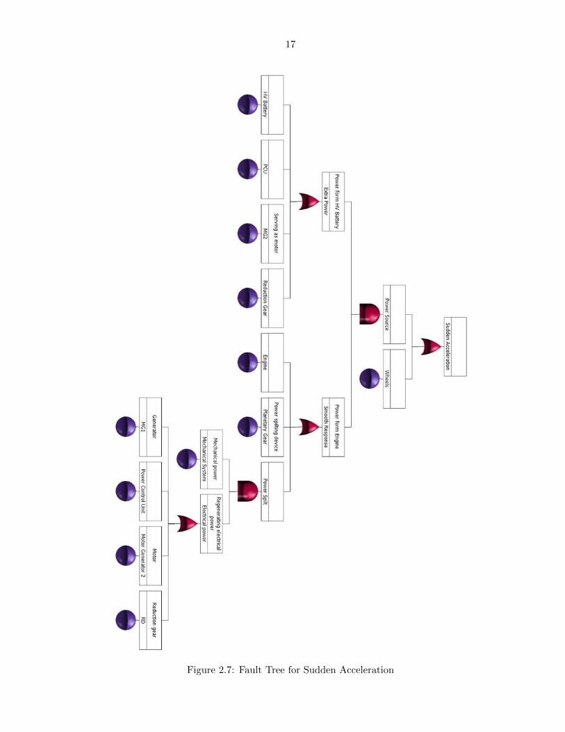


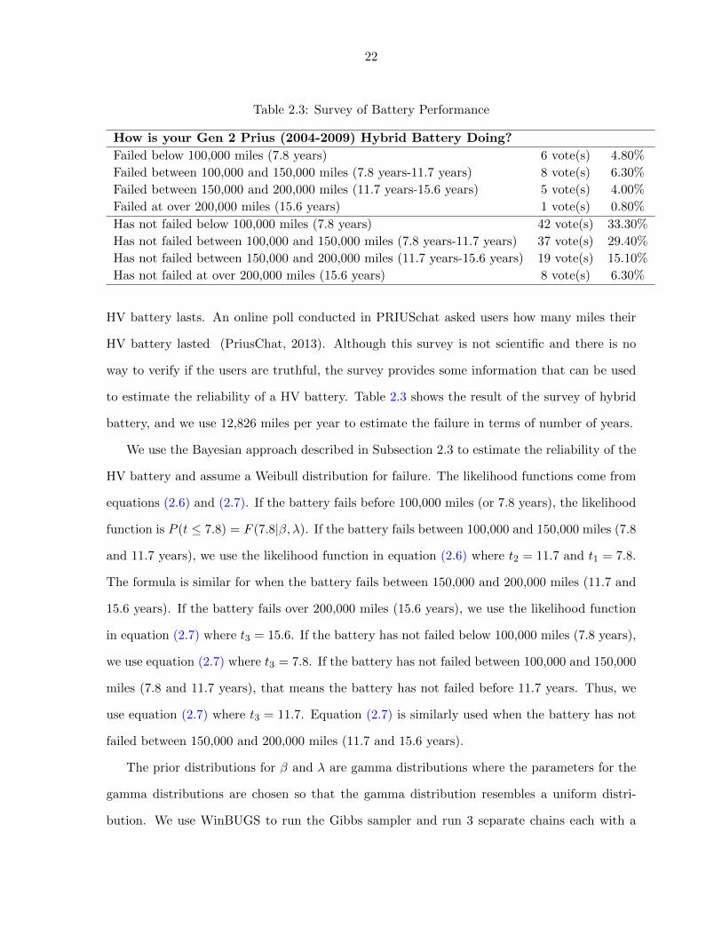


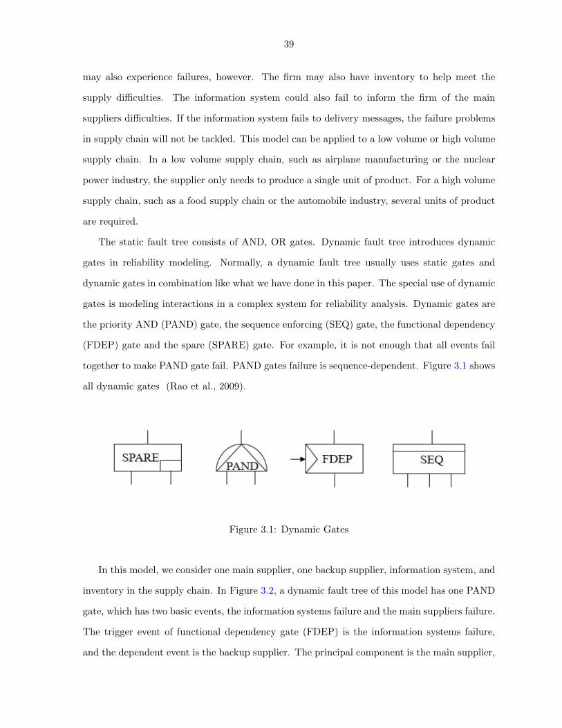


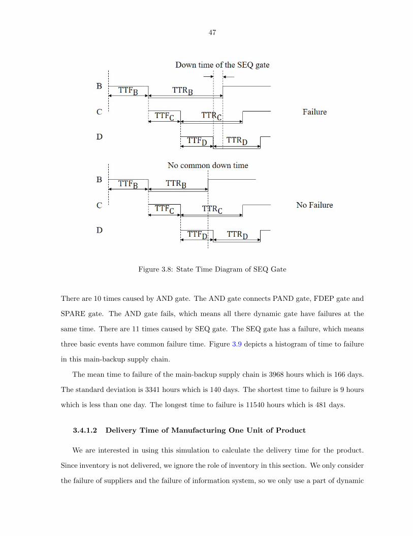


![Fault Tree Diagram[1]](https://static.documents.pub/doc/80x56/55cf8c8a5503462b138d7284/fault-tree-diagram1.jpg)

