Static and Dynamic Human Shape Modeling … Static and Dynamic Human Shape Modeling – Concept...

AFRL-RH-WP-TR-2011-0023

Static and Dynamic Human Shape Modeling – Concept

Formation and Technology Development

Zhiqing Cheng

Infoscitex Corporation

Julia Parakkat

Melody Darby

Kathleen Robinette

Vulnerability Analysis Branch

Biosciences and Performance Division

FEBRUARY 2011

Final Report

Distribution A: Approved for public release; distribution is unlimited.

See additional restrictions described on inside pages

AIR FORCE RESEARCH LABORATORY

711TH

HUMAN PERFORMANCE WING

HUMAN EFFECTIVENESS DIRECTORATE

WRIGHT-PATTERSON AIR FORCE BASE, OH 45433

AIR FORCE MATERIEL COMMAND

UNITED STATES AIR FORCE

NOTICE AND SIGNATURE PAGE

\"'sing Government drawings, specifications, or olher dala incllJ(led in this document for any purpose other lhan Government procurement does not in an) way obligate lhe U,S, Govcl11J11cni. The fact that the Government formulated or supplied the ara\\ ings, specifications, or other data docs not license the holder or any other person or corporation: or convey any rights or permission to manufacture. use. or sell any patented invention thai m<1)- relate to them,

This report "as cleared for public release by the 88th Air Base V,:ing Public Affairs Office and IS

3\ailable to the general public, including fo reign nationals, Copies ma) be oblained trom the Defense Technical Information Center (DTlC) (imp:!/w\\'\\,dtic,mil),

AFRL-RH-WP-TR-2011-0023 HAS BEEN REVIEWED AND IS APPROVED FOR PUBLICATION IN ACCORDANCE WITII ASSIGl\ED DISTRIBUTIO" STA II-,MI:Sr.

.Iulia Parak"a!. Work Unit vtanager Vulnerab ility Analysis Branch

This repon is published in the intcrcst of scienti fie and technical int()fJnatiol1 exchangc, and its publication does not constitute the Government's approval or tlisapprO\al or its ideas or tinding~.

REPORT DOCUMENTATION PAGE Form Approved

OMB No. 0704-0188 Public reporting burden for this collection of information is estimated to average 1 hour per response, including the time for reviewing instructions, searching existing data sources, gathering and maintaining the data needed, and completing and reviewing this collection of information. Send comments regarding this burden estimate or any other aspect of this collection of information, including suggestions for reducing this burden to Department of Defense, Washington Headquarters Services, Directorate for Information Operations and Reports (0704-0188), 1215 Jefferson Davis Highway, Suite 1204, Arlington, VA 22202-4302. Respondents should be aware that notwithstanding any other provision of law, no person shall be subject to any penalty for failing to comply with a collection of information if it does not display a currently valid OMB control number. PLEASE DO NOT RETURN YOUR FORM TO THE ABOVE ADDRESS.

1. REPORT DATE (DD-MM-YYYY)

02-28-2011 2. REPORT TYPE

Final 3. DATES COVERED (From - To)

January 2009 – February 2011

4. TITLE AND SUBTITLE

Static and Dynamic Human Shape Modeling – Concept Formation and

Technology Development

5a. CONTRACT NUMBER

IN-HOUSE 5b. GRANT NUMBER

5c. PROGRAM ELEMENT NUMBER

62202F 6. AUTHOR(S)

Zhiqing Cheng, Julia Parakkat, Melody Darby, Kathleen Robinette

5d. PROJECT NUMBER

7184 5e. TASK NUMBER

02 5f. WORK UNIT NUMBER

71840226 7. PERFORMING ORGANIZATION NAME(S) AND ADDRESS(ES)

8. PERFORMING ORGANIZATION REPORT

NUMBER



Air Force Research Laboratory

9. SPONSORING / MONITORING AGENCY NAME(S) AND ADDRESS(ES) 10. SPONSOR/MONITOR’S ACRONYM(S)

Air Force Materiel Command

Air Force Research Laboratory

711th Human Performance Wing

Human Effectiveness Directorate



Wright-Patterson AFB OH 45433-7947

711 HPW/RHPA

11. SPONSOR/MONITOR’S REPORT

NUMBER(S)

AFRL-RH-WP-TR-2011-0023

12. DISTRIBUTION / AVAILABILITY STATEMENT

Distribution A: Approved for public release, distribution is unlimited

13. SUPPLEMENTARY NOTES

88ABW/PA cleared on 31 Mar 11, 88ABW-2011-1953

14. ABSTRACT

Extensive investigations were performed in this project on human shape modeling. The problem was addressed

from the perspectives of static shape modeling and morphing, human shape modeling in various poses, dynamic

modeling, and human activity replication/ animation. The major problems involved in each topic were identified,

and the methods and techniques were developed or formulated for them. Some of these methods or algorithms

were implemented, and the results were presented and discussed. Conclusions were drawn from research results

and findings, the issues remaining were described, and the future work was discussed.

15. SUBJECT TERMS

Static Human Shape Modeling; Pose Change Modeling; Dynamic 3-D Human Shape Modeling, Human Activity

Replication/Animation 16. SECURITY CLASSIFICATION OF:

17. LIMITATION

OF ABSTRACT

18. NUMBER

OF PAGES

19a. NAME OF RESPONSIBLE PERSON

Julia Parakkat a. REPORT

U

b. ABSTRACT

U

c. THIS PAGE

U

SAR 36 19b. TELEPHONE NUMBER (include area

code)

NA Standard Form 298 (Rev. 8-98)

Prescribed by ANSI Std. 239.18

i

ii

THIS PAGE IS INTENTIONAL LEFT BLANK

iii

TABLE OF CONTENTS

SUMMARY .................................................................................................................................... v 1.0 INTRODUCTION .............................................................................................................. 1 2.0 STATIC SHAPE MODELING AND MORPHING........................................................... 1

2.1 Joint Center Calculation ................................................................................................... 2 2.2 Skeleton model building................................................................................................... 3 2.3 Segmentation .................................................................................................................... 3 2.4 Slicing............................................................................................................................... 4 2.5 Discretizing ...................................................................................................................... 4

2.6 Hole filling ....................................................................................................................... 5 2.7 Parameterization and shape description ........................................................................... 5 2.8 Surface Registration ......................................................................................................... 6 2.9 Shape Variation Characterization Using PCA ................................................................. 6 2.10 Feature Extraction with Control Parameters ................................................................ 7 2.11 Shape Reconstruction/Morphing .................................................................................. 8

2.11.1 Morphing between two examples ............................................................................. 8 2.11.2 Interpolation in a multi-dimensional space ............................................................... 9 2.11.3 Reconstruction from Eigen space ............................................................................. 9 2.11.4 Feature-based Synthesis .......................................................................................... 10

2.12 Part blending ............................................................................................................... 10

3.0 HUMAN SHAPE MODELING IN VARIOUS POSES .................................................. 11 3.1 Problem Analysis and Approach Formation .................................................................. 11 3.2 Data Collection and Processing...................................................................................... 12 3.3 Pose Deformation Modeling .......................................................................................... 13

3.3.1 Coordinate Transformation ..................................................................................... 14 3.3.2 Surface Deformation Characterization ................................................................... 15 3.3.3 Surface Deformation Representation ...................................................................... 19 3.3.4 Surface Deformation Prediction ............................................................................. 19 3.3.5 Body Shape Prediction for New Poses ................................................................... 19

4.0 DYNAMIC MODELING ................................................................................................. 20

4.1 General Considerations .................................................................................................. 20 4.2 Template Model ............................................................................................................. 21 4.3 Instance Model ............................................................................................................... 22 4.4 Model fitting ................................................................................................................... 22

4.5 Iteration .......................................................................................................................... 24 4.6 Computation Efficiency ................................................................................................. 24

5.0 REPLICATION AND ANIMATION............................................................................... 25 5.1 Replication ..................................................................................................................... 25 5.2 Animation ....................................................................................................................... 25

5.2.1 Using marker data directly ...................................................................................... 25

5.2.2 Using joint angles ................................................................................................... 26

6.0 CONCLUDING REMARKS ............................................................................................ 27 7.0 REFERENCES ................................................................................................................. 28 8.0 GLOSSARY/ACRONYMS .............................................................................................. 30

iv

LIST OF FIGURES

Figure 1. Landmarks, joint centers, and skeleton model ............................................................. 3

Figure 2. Segmentation and slicing .............................................................................................. 4

Figure 3. Discretizing contour lines ............................................................................................. 5

Figure 4. Hole filling .................................................................................................................... 5

Figure 5. Control parameters of body shape ................................................................................ 8

Figure 6. Morphing from a male to a female ............................................................................... 9

Figure 7. A semantic structure for shape reconstruction ........................................................... 10

Figure 8. The framework of a pose modeling technology ......................................................... 12

Figure 9. A template model for pose modeling ......................................................................... 14

Figure 10. Eigen value ratio for all 16 segments ....................................................................... 16

Figure 11. Shape reconstruction using principal components ................................................... 17

Figure 12. Sum of squre errors of shape reconstruction ............................................................ 18

Figure 13. Predicted shape in 8 different poses ......................................................................... 20

Figure 14. A scheme for dynamic modeling .............................................................................. 21

Figure 15. Cost function ............................................................................................................ 23

Figure 16. An example of replication ........................................................................................ 25

Figure 17. An example of marker-based animation ................................................................... 26

Figure 18. Human motion replication in 3-D space/Virtual activity creation ........................... 27

v

SUMMARY

This report details the research performed on human shape modeling. The topics covered include

static shape modeling and morphing, human shape modeling in various poses, dynamic

modeling, and human activity replication/animation. The report provides a detailed description

of the challenges of each topic, the methods and algorithms developed for each topic, the

implementation of the methods and algorithms developed, and some computational results. The

contents of the report are arranged as follows: 1. Introduction; 2. Static Shape Modeling and

Morphing; 3. Shape Modeling in Various Poses; 4. Dynamic Modeling; 5. Human Activity

Replication and Animation; 6. Concluding Remarks; and 7. References.

vi

THIS PAGE IS INTENTIONAL LEFT BLANK

1


1.0 INTRODUCTION

Human modeling and simulation has vast applications in various areas, such as immersive and

interactive virtual reality, human-machine interface and work station, game and entertainment,

human identification, and human-borne threat detection. However, creating a realistic,

morphable, animatable, and highly bio-fidelic human shape model is a major challenge for

anthropometry and computer graphics.

Human shape modeling can be classified as either static or dynamic. Static shape modeling

creates a model to describe human shape at a particular pose, usually a standing pose. The major

issues involved in static shape modeling include shape description, registration, hole filling,

shape variation characterization, and shape reconstruction. Dynamic shape modeling addresses

shape variations due to pose changes or due to gross body motion. While pose identification,

skeleton modeling, and shape deformation are the major issues involved with pose modeling,

motion tracking, shape extraction, shape reconstruction, animation, and inverse kinematics are

the main issues to consider for the shape modeling of humans in motion.

A static three dimensional (3-D) human shape model provides anthropometric information. A

dynamic 3-D human shape model contains information on shape, pose, and gait. Constructed

from 2-D video imagery or 3-D sensor data, such a model can potentially be used to depict a

human’s activity and behavior, to predict his intention, to uncover any disguises, and to uncover

hidden objects. Therefore, human shape modeling technology can be used for suspect

identification and human-borne threat detection, in addition to its traditional applications, such as

ergonomic design of human spaces and workstations, creating vivid and realistic figures and

action animations, and virtual design and fitting of personalized clothing.

As human modeling and simulation play a critical role in human identification and human-borne

threat detection, a 6.2 program entitled, “Human Measurement Modeling,” was established in the

Air Force Research Laboratory for research on human shape modeling. Under the support of this

program, extensive investigations were performed on static shape modeling and morphing, shape

modeling in various poses (pose modeling), dynamic modeling, and human activity replication

and animation. In a preceding report [1], a literature review was presented on recent

developments in human shape modeling, in particular, static shape modeling based on range scan

data and dynamic shape modeling from video imagery. This report describes the investigations

on the methodology development, concept formation, solution formulation, and algorithm

development and implementation.

2.0 STATIC SHAPE MODELING AND MORPHING

The 3-D human static shape modeling in this project is based on the 3-D laser scan data from the

CAESAR (Civilian American and European Surface Anthropometry Resource) database

(http://store.sae.org/caesar). For the representation of a human body shape, polygons/vertices are

usually used as the basic graphic entities. Approximately 20,000 ~ 500,000 vertices are required

to describe a full body shape, depending upon surface resolution. This method of surface

representation incurs a large computational cost and cannot ensure point-to-point correspondence

among the scans of different subjects. Instead, contour lines were proposed as the basic entities

http://store.sae.org/caesar

2


for the shape modeling in this project. The entire procedure for static shape modeling consists of

several steps: (1) joint center calculation; (2) skeleton model building; (3) segmentation; (4)

slicing; (5) discretizing; (6) hole filling; (7) parameterization and shape description; (8) surface

registration; (9) shape variation characterization using Principle Component Analysis (PCA);

(10) feature extraction with control parameters; (11) shape reconstruction/morphing; and (12)

part blending. The details of each step are described below.

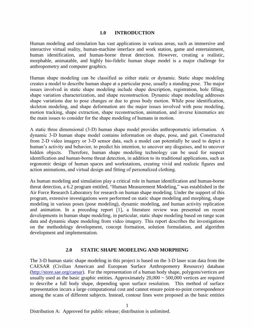
2.1 Joint Center Calculation

The human body is treated as a multi-segment system where segments are connected to each

other by joints. The joint centers are defined by respective landmarks, which in turn, are either

measured or calculated in the CAESAR database. According to [2], major joint centers are

defined by landmarks as follows:

Ankles, right and left: use midpoint between Lateral Malleolus and Sphyrion.

Knees, right and left: use midpoint between Lateral and Medial Femoral Epicondyles.

Hips, right and left: 1) start at midpoint between Anterior Superior Iliac Spine and

Symphysion;

2) translate in the posterior direction to the plane of the Trochanterions;

3) translate 15 mm down.

Pelvic Joint: 1) start at Posterior Superior Iliac Midspine coordinates;

2) translate 51 mm in the anterior direction.

Abdomen Joint: 1) start at 10th

Rib Midspine coordinates;

2) translate 51 mm in the anterior direction.

Thorax Joint: 1) start at Cervicale coordinates;

2) translate 51 mm in the anterior direction;


Head/Neck Joint: use midpoint between right and left Tragions.

Shoulder, right and left: 1) start at Acromion coordinates;

2) translate 38 mm in the medial direction;


Elbow, right and left: use midpoint between Medial and Lateral Humeral Epicondyles

Wrist, right and left: use midpoint between Radial and Ulnar Styloid Processes

According to the 3-D landmark list for standing posture used in the CAESAR database [3], a

Matlab code was developed to calculate the joints centers. Figure 1 illustrates an example of the

joint centers derived from landmarks.

3


Figure 1. Landmarks, joint centers, and skeleton model

2.2 Skeleton model building

A skeleton model is built by connecting respective joint centers to represent the articulated

structure and segments of human body, as shown in Figure 1. Note that while the skeleton model

thus defined works well for static shape modeling, it may not be suitable for pose changing

modeling or dynamic shape modeling, because in the latter cases the joint centers need to

describe the true kinematics of human body motion.

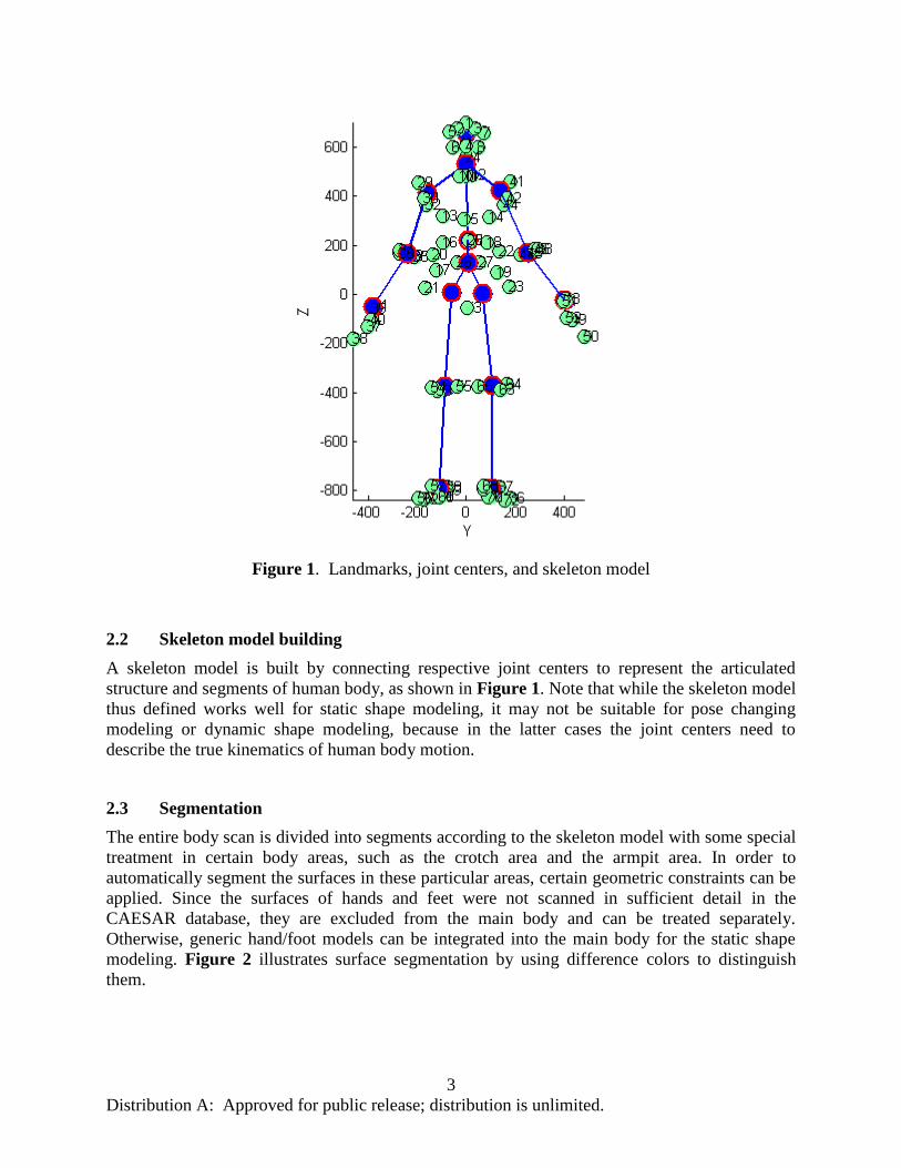
2.3 Segmentation

The entire body scan is divided into segments according to the skeleton model with some special

treatment in certain body areas, such as the crotch area and the armpit area. In order to

automatically segment the surfaces in these particular areas, certain geometric constraints can be

applied. Since the surfaces of hands and feet were not scanned in sufficient detail in the

CAESAR database, they are excluded from the main body and can be treated separately.

Otherwise, generic hand/foot models can be integrated into the main body for the static shape

modeling. Figure 2 illustrates surface segmentation by using difference colors to distinguish

them.

4


Figure 2. Segmentation and slicing

2.4 Slicing

The scan of each segment is sliced along the main axis of each segment at fixed intervals, which

produces the contour lines of the segment, as shown in Figure 2. The interval length for each

segment varies depending upon the surface variation and area.

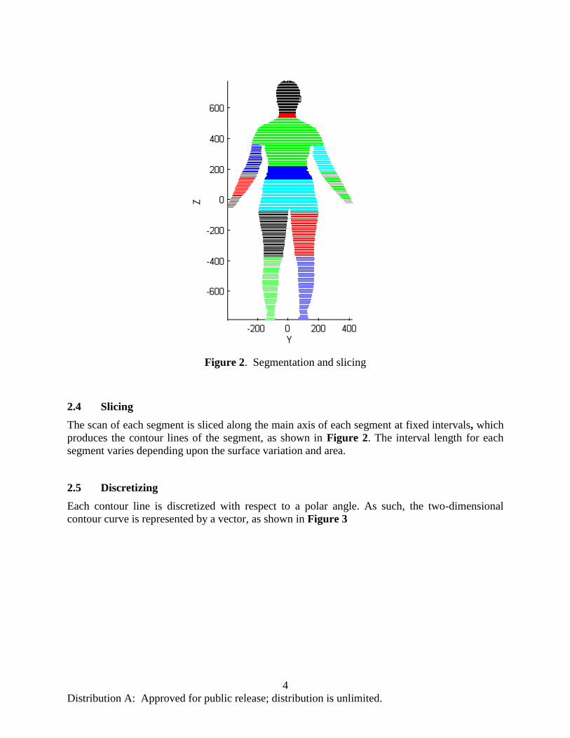
2.5 Discretizing

Each contour line is discretized with respect to a polar angle. As such, the two-dimensional

contour curve is represented by a vector, as shown in Figure 3

5


Figure 3. Discretizing contour lines

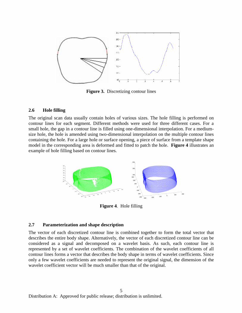
2.6 Hole filling

The original scan data usually contain holes of various sizes. The hole filling is performed on

contour lines for each segment. Different methods were used for three different cases. For a

small hole, the gap in a contour line is filled using one-dimensional interpolation. For a medium-

size hole, the hole is amended using two-dimensional interpolation on the multiple contour lines

containing the hole. For a large hole or surface opening, a piece of surface from a template shape

model in the corresponding area is deformed and fitted to patch the hole. Figure 4 illustrates an

example of hole filling based on contour lines.

Figure 4. Hole filling

2.7 Parameterization and shape description

The vector of each discretized contour line is combined together to form the total vector that

describes the entire body shape. Alternatively, the vector of each discretized contour line can be

considered as a signal and decomposed on a wavelet basis. As such, each contour line is

represented by a set of wavelet coefficients. The combination of the wavelet coefficients of all

contour lines forms a vector that describes the body shape in terms of wavelet coefficients. Since

only a few wavelet coefficients are needed to represent the original signal, the dimension of the

wavelet coefficient vector will be much smaller than that of the original.

-300-200

-1000

100200

-300

-200

-100

0

100

200

300

150

200

250

6


2.8 Surface Registration

After the same schemes of segmentation, slicing, discretizing, and parameterization are applied

to different scans (subjects), the point-to-point correspondence among the scans of different

bodies is established. This presents a way for surface registration.

2.9 Shape Variation Characterization Using PCA

Principal component analysis (PCA) is a major method often used to characterize human shape

variations. Suppose

LlKkNnckl

mnm,1;,1;,1},{ S

(1)

is a shape descriptor , where m=1, ..., M denotes each subject, n=1, …, N points to each segment

of a subject, k=1, …, K describes each contour line of a segment, and l=1, …, L refers to each

point of a contour line (or each wavelet coefficients if each contour line is expanded in terms of

wavelets). Conventional PCA of shape m

S is described as follows:

DUVV

AAU

SSSA

SSS

SS

1

21

1

]~~~

[

~

T

M

mmm

M

mmm

, (2)

where UDUV of eseigen valu theare )diag( and of orseigen vect thecontains . However, a problem with

this approach is that as each m

S may contain thousands of elements, U is a matrix with huge size

that can easily exceeds the capacity of computer memory.

In order to cope with this problem, a method called incremental principal component analysis

(IPCA) can be used. However, it has several potential problems also. Alternatively, a special

treatment can be implemented on the conventional PCA. Denote

AACT'

, (3)

as a new covariance matrix with much smaller size (whose dimension equals the number of

observations). The eigen values of '

C are given by ''''

DVCV1

, (4)

where '

V contains eigen vectors and diag('

D ) are eigen values. From Eq. (4) it follows that ''''

VDVC , (5)

that is,

iii d ''''vvC , (6)

or

iiiT d '''

vAvA . (7)

Further,

7


iiiT d '''

AvAvAA . (8)

That is

iii d '''AvCAv . (9)

Let

ii

'Avv , (10)

and '

i 'idd , (11)

Or '

AVV (12) '

DD . (13)

Further, V needs to be normalized by 2/1'' )(* DAVV abs . (14)

The principal components of A are given by Eq. (12). Since '

C is usually much smaller thanC ,

the PCA becomes tractable for the capacity of computer memory.

While the body shape variation can be characterized with respect to the entire population, certain

features or characteristics are uniquely associated with gender, ethnicity, age, and some other

classifiers. Conversely, these unique body features can provide useful clues about a subject of

interest. Therefore, PCA can be conducted on particular cases, such as

Case-1: Overall PCA: all subjects in the database as one group;

Case-2: Group PCA: subjects grouped according to gender;

Case-3: Group PCA: subjects grouped according to age band;

Case-4: Group PCA: Subjects grouped according to ethnicity.

2.10 Feature Extraction with Control Parameters

Principal component analysis helps to characterize the space of human body variation, but it does

not provide a direct way to explore the range of bodies with intuitive control parameters, such as

height and weight. Allen et al [4] showed how to relate several variables simultaneously by

learning a linear mapping between the control parameters and the PCA weights. Ben Azouz et al

[5] attempted to link the principal modes to some intuitive body shape variations by visualizing

the first five modes of variation and giving interpretations of these modes. Alternatively, sizing

parameters or anthropometric measurements can be used to control the body shape. However,

providing all measurements that are sufficient to describe a detailed shape model would be

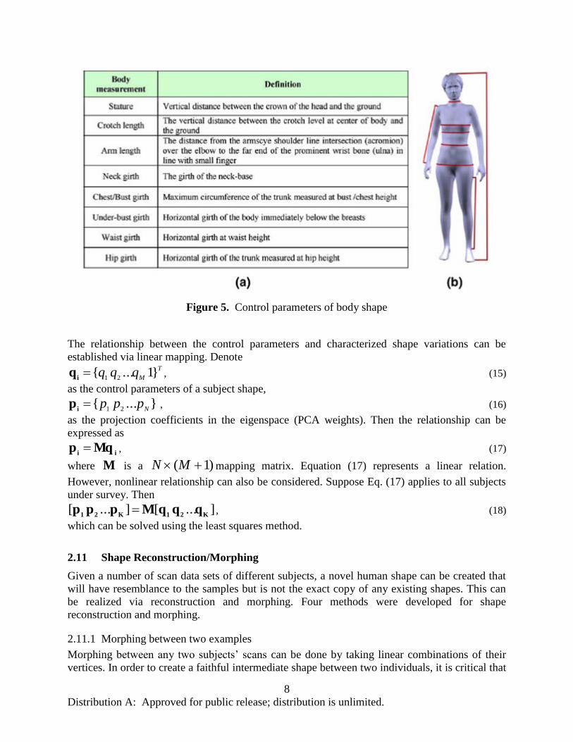
almost impractical. Instead, eight anthropometric measurements (5 girths and 3 lengths) were

used as sizing parameters in this project, as displayed in Figure 5. These eight primary

measurements have been defined as the primary body measurements for product-independent

size assignment [6] and were used by Seo et al [7] for human shape synthesizing. Using such a

small measurement set provides compact, easily obtainable parameters for the body geometry

representation, enabling applications such as an online clothing store, where a user is asked to

enter his/her measurements for customized apparel design. Because landmark data were

collected and provided in the CAESAR database, these size parameters can be calculated for

each subject using landmark data.

8


Figure 5. Control parameters of body shape

The relationship between the control parameters and characterized shape variations can be

established via linear mapping. Denote T

Mqqq }1...{

21

iq , (15)

as the control parameters of a subject shape,

}...{21 N

pppi

p , (16)

as the projection coefficients in the eigenspace (PCA weights). Then the relationship can be

expressed as

iiMqp , (17)

where M is a )1( MN mapping matrix. Equation (17) represents a linear relation.

However, nonlinear relationship can also be considered. Suppose Eq. (17) applies to all subjects

under survey. Then

]...[]...[K21K21

qqqMppp , (18)

which can be solved using the least squares method.

2.11 Shape Reconstruction/Morphing

Given a number of scan data sets of different subjects, a novel human shape can be created that

will have resemblance to the samples but is not the exact copy of any existing shapes. This can

be realized via reconstruction and morphing. Four methods were developed for shape

reconstruction and morphing.

2.11.1 Morphing between two examples

Morphing between any two subjects’ scans can be done by taking linear combinations of their

vertices. In order to create a faithful intermediate shape between two individuals, it is critical that

9


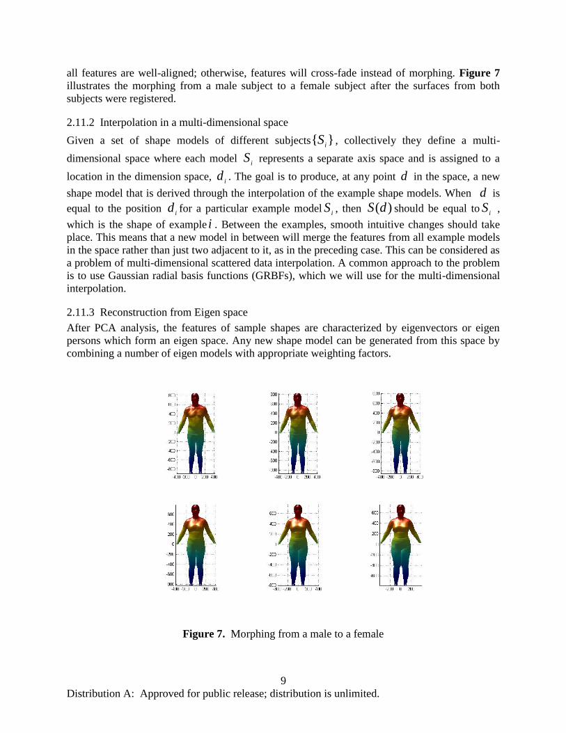
all features are well-aligned; otherwise, features will cross-fade instead of morphing. Figure 7

illustrates the morphing from a male subject to a female subject after the surfaces from both

subjects were registered.

2.11.2 Interpolation in a multi-dimensional space

Given a set of shape models of different subjects }{i

S , collectively they define a multi-

dimensional space where each model i

S represents a separate axis space and is assigned to a

location in the dimension space, i

d . The goal is to produce, at any point d in the space, a new

shape model that is derived through the interpolation of the example shape models. When d is

equal to the position i

d for a particular example modeli

S , then )(dS should be equal toi

S ,

which is the shape of example i . Between the examples, smooth intuitive changes should take

place. This means that a new model in between will merge the features from all example models

in the space rather than just two adjacent to it, as in the preceding case. This can be considered as

a problem of multi-dimensional scattered data interpolation. A common approach to the problem

is to use Gaussian radial basis functions (GRBFs), which we will use for the multi-dimensional

interpolation.

2.11.3 Reconstruction from Eigen space

After PCA analysis, the features of sample shapes are characterized by eigenvectors or eigen

persons which form an eigen space. Any new shape model can be generated from this space by

combining a number of eigen models with appropriate weighting factors.

Figure 6. Morphing from a male to a female

Figure 7. Morphing from a male to a female

10


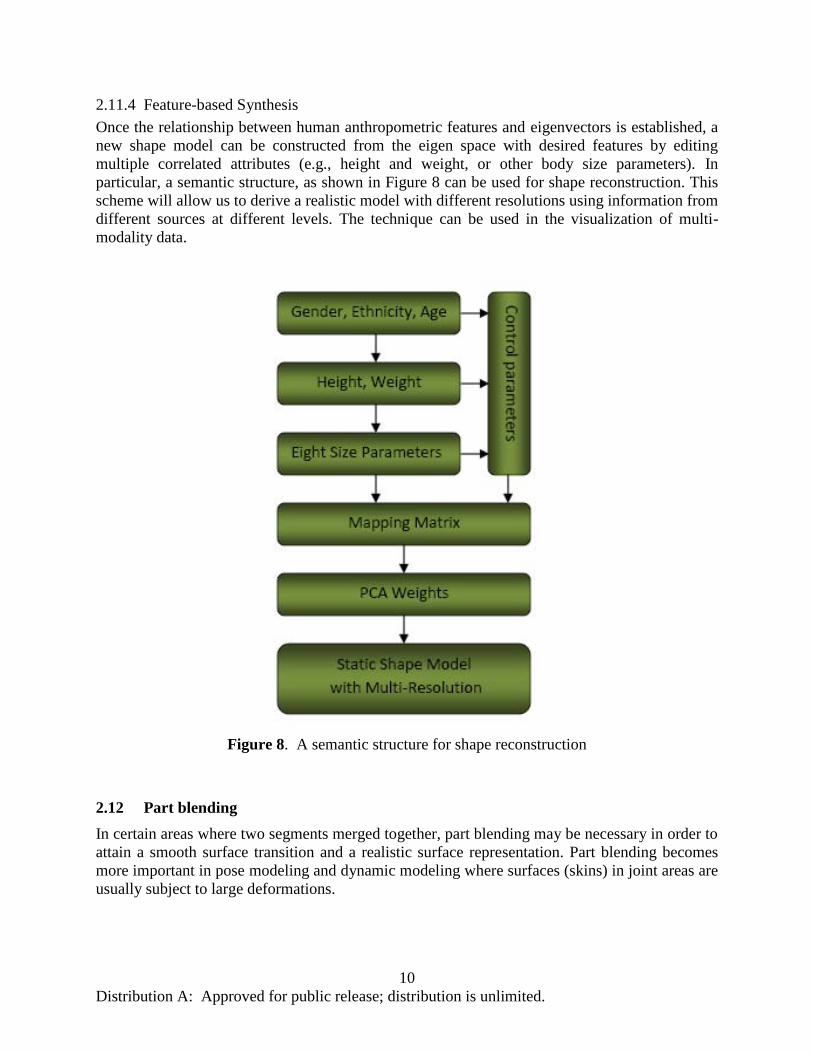
2.11.4 Feature-based Synthesis

Once the relationship between human anthropometric features and eigenvectors is established, a

new shape model can be constructed from the eigen space with desired features by editing

multiple correlated attributes (e.g., height and weight, or other body size parameters). In

particular, a semantic structure, as shown in Figure 8 can be used for shape reconstruction. This

scheme will allow us to derive a realistic model with different resolutions using information from

different sources at different levels. The technique can be used in the visualization of multi-

modality data.

Figure 8. A semantic structure for shape reconstruction

2.12 Part blending

In certain areas where two segments merged together, part blending may be necessary in order to

attain a smooth surface transition and a realistic surface representation. Part blending becomes

more important in pose modeling and dynamic modeling where surfaces (skins) in joint areas are

usually subject to large deformations.

11


3.0 HUMAN SHAPE MODELING IN VARIOUS POSES

3.1 Problem Analysis and Approach Formation

In order to develop feasible and effective pose modeling methods, a general analysis of the

problem is in order.

• The human body is an articulated structure. That is, the human body can be treated as a

system of segments linked by joints.

• The human pose changes as the joints rotate. Therefore, a pose can be defined in terms of

respective joint angles.

• The body shape varies in different poses. The variations are caused by two factors: the

articulated motion of each segment and the surface deformation of each segment.

• It can be reasonably assumed that the surface deformation of a segment depends only on the

rotations of the joint(s) adjacent to the segment. While the surface deformation of certain

body regions may still be affected by the rotations of joints that are not directly connected,

this assumption is valid for most regions of the human body and thus is often used.

Based on the above analyses, a framework for pose modeling was formulated, as shown in

Figure 9. The core part of pose modeling is to establish a mapping matrix that can be used to

predict and construct the body shape model of a particular person at a particular pose. Therefore,

in the true meaning of pose modeling, the mapping matrix needs to represent the shape changes

not only due to body variations of different human and pose deformations at different poses

independently, but also resulting from the cross correlations between identity and pose. In

reality, it is not feasible to determine the relationship between the pose deformation and the body

shape variation using PCA in the same way as used for shape variation analysis, since it is too

costly to collect pose data for a large number of subjects. Alternatively, it is possible to collect

pose data for several typical subjects (e.g., male, female, tall, short, big, and small) who are

selected to represent the entire population. For a particular subject, the mapping matrix for

his/her pose deformation can be determined by subject classification based on certain criteria

such as nearest neighborhood.

12


Figure 9. The framework of a pose modeling technology

3.2 Data Collection and Processing

In order to create a morphable (for different subjects), deformable (for different poses), 3-D

model of human body shape, it is necessary to collect many samples of human shape and pose.

Properly sampling the entire range of human body shapes and poses is important to creating a

robust model. The CAESAR (Civilian American and European Surface Anthropometry

Resource) database provides human shape data for thousands of subjects in three poses. It can be

used to train a static shape model and to represent human shape variation. The data sets that are

required to establish a pose mapping matrix and to train pose models are not publicly available.

The data used in this research, however, was collected by Anguelov et al [8] from one subject in

70 poses.

In order to use the pose data for pose modeling, data processing is usually required. It includes

three major tasks: hole-filling, point-to-point registration, and automatic surface segmentation.

Hole-filling Polygonal meshes that are derived from laser scanners frequently have missing

data for regions where the laser neither reached nor produced adequate reflectance. This

problem occurs more often when a subject is not in the standard pose (the standing pose used

13


in the CAESAR database). Interpolating data into these regions often goes by the name of

hole-filling. Several methods have been developed for hole-filling, such as the volumetric

method [9].

Point-to-point registration Polygonal mesh surfaces of the same object, but taken during

different scans are not naturally in correspondence. In order to form complete models it is

necessary to find this correspondence, i.e., which point on surface A corresponds to which

point on surface B. Non-rigid registration is required to bring 3-D meshes of people in

different poses into alignment. While many academic papers have been published which

describe fully automated methods [10, 11], the complexity of the problem often leads to

optimization prone to local minima. Thus most of these methods tend to lack sufficient

robustness for unattended real world applications. Fortunately, establishing correspondence

of a few control points by hand is usually sufficient to insure convergence. Labeling more

points insures better convergence.

Automatic surface segmentation Given a deformable surface with multiple poses brought into

correspondence, it is possible to segment the surface into disjoint regions. Each of these

regions approximates a rigid articulated segment of the human body [12, 13]. The easiest

way to achieve segmentation is to observe that polygons in the same segment tend to move

together, that is, their rotation and translation are the same for a given pair of poses. By

performing a K-means clustering over all polygons in all poses, and enforcing continuity of

segments, the best segmentation is obtainable.

3.3 Pose Deformation Modeling

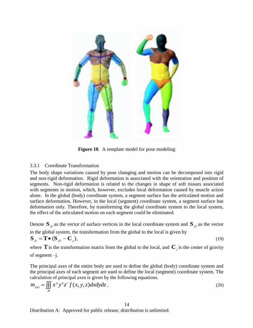
The template model associated with the pose dataset consists of 16 segments, each of which has

the pre-defined surface division, as shown in Figure 10 [8]. Identifying the surface for each

segment in different poses and establishing point-to-point correspondence for each surface in all

observed poses is essential to the pose modeling. The method developed for pose deformation

modeling in this paper consists of multiple steps, which are described below.

14


Figure 10. A template model for pose modeling

3.3.1 Coordinate Transformation

The body shape variations caused by pose changing and motion can be decomposed into rigid

and non-rigid deformation. Rigid deformation is associated with the orientation and position of

segments. Non-rigid deformation is related to the changes in shape of soft tissues associated

with segments in motion, which, however, excludes local deformation caused by muscle action

alone. In the global (body) coordinate system, a segment surface has the articulated motion and

surface deformation. However, in the local (segment) coordinate system, a segment surface has

deformation only. Therefore, by transforming the global coordinate system to the local system,

the effect of the articulated motion on each segment could be eliminated.

Denote jL

S as the vector of surface vertices in the local coordinate system and jG

S as the vector

in the global system, the transformation from the global to the local is given by

)(jjGjL

CSTS , (19)

where T is the transformation matrix from the global to the local, and j

C is the center of gravity

of segment –j.

The principal axes of the entire body are used to define the global (body) coordinate system and

the principal axes of each segment are used to define the local (segment) coordinate system. The

calculation of principal axes is given by the following equations.

M

rqp

pqrdxdydzzyxfzyxm ),,( , (20)

15


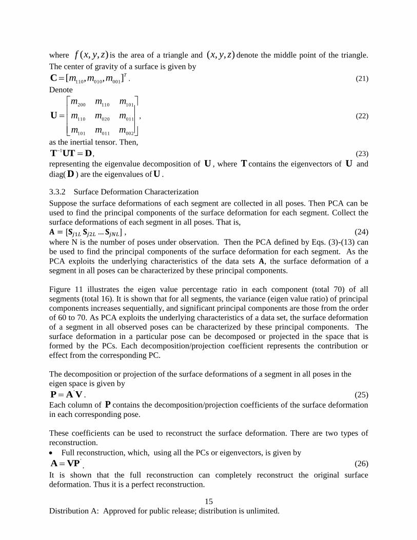
where ),,( zyxf is the area of a triangle and ),,( zyx denote the middle point of the triangle.

The center of gravity of a surface is given by Tmmm ],,[

001010110C . (21)

Denote

002011101

011020110

101110200

mmm

mmm

mmm

U , (22)

as the inertial tensor. Then,

DUTT 1, (23)

representing the eigenvalue decomposition of U , where T contains the eigenvectors of U and

diag( D ) are the eigenvalues of U .

3.3.2 Surface Deformation Characterization

Suppose the surface deformations of each segment are collected in all poses. Then PCA can be

used to find the principal components of the surface deformation for each segment. Collect the

surface deformations of each segment in all poses. That is,

, (24)

where N is the number of poses under observation. Then the PCA defined by Eqs. (3)-(13) can

be used to find the principal components of the surface deformation for each segment. As the

PCA exploits the underlying characteristics of the data sets , the surface deformation of a

segment in all poses can be characterized by these principal components.

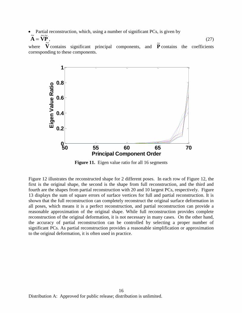
Figure 11 illustrates the eigen value percentage ratio in each component (total 70) of all

segments (total 16). It is shown that for all segments, the variance (eigen value ratio) of principal

components increases sequentially, and significant principal components are those from the order

of 60 to 70. As PCA exploits the underlying characteristics of a data set, the surface deformation

of a segment in all observed poses can be characterized by these principal components. The

surface deformation in a particular pose can be decomposed or projected in the space that is

formed by the PCs. Each decomposition/projection coefficient represents the contribution or

effect from the corresponding PC.

The decomposition or projection of the surface deformations of a segment in all poses in the

eigen space is given by

VAP' . (25)

Each column of P contains the decomposition/projection coefficients of the surface deformation

in each corresponding pose.

These coefficients can be used to reconstruct the surface deformation. There are two types of

reconstruction.

Full reconstruction, which, using all the PCs or eigenvectors, is given by '

VPA . (26)

It is shown that the full reconstruction can completely reconstruct the original surface

deformation. Thus it is a perfect reconstruction.

16


Partial reconstruction, which, using a number of significant PCs, is given by

'~~~

PVA , (27)

where V~

contains significant principal components, and P~

contains the coefficients

corresponding to these components.

Figure 11. Eigen value ratio for all 16 segments

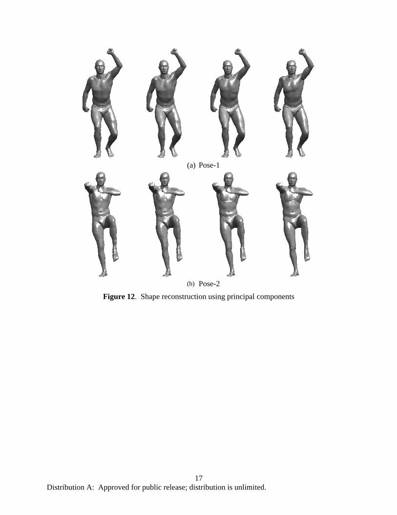
Figure 12 illustrates the reconstructed shape for 2 different poses. In each row of Figure 12, the

first is the original shape, the second is the shape from full reconstruction, and the third and

fourth are the shapes from partial reconstruction with 20 and 10 largest PCs, respectively. Figure

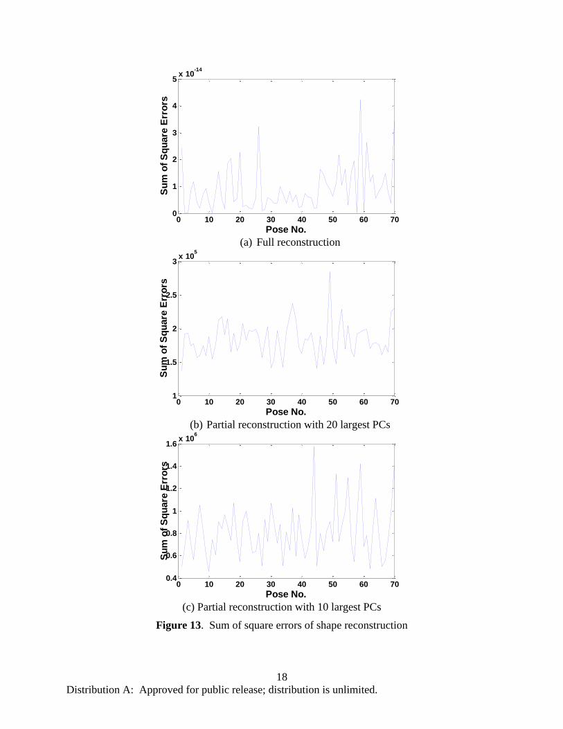
13 displays the sum of square errors of surface vertices for full and partial reconstruction. It is

shown that the full reconstruction can completely reconstruct the original surface deformation in

all poses, which means it is a perfect reconstruction, and partial reconstruction can provide a

reasonable approximation of the original shape. While full reconstruction provides complete

reconstruction of the original deformation, it is not necessary in many cases. On the other hand,

the accuracy of partial reconstruction can be controlled by selecting a proper number of

significant PCs. As partial reconstruction provides a reasonable simplification or approximation

to the original deformation, it is often used in practice.

50 55 60 65 700

0.2

0.4

0.6

0.8

1

Principal Component Order

Eig

en

Valu

e R

ati

o

17


(a) Pose-1

(b) Pose-2

Figure 12. Shape reconstruction using principal components

18


(a) Full reconstruction

(b) Partial reconstruction with 20 largest PCs

(c) Partial reconstruction with 10 largest PCs

Figure 13. Sum of square errors of shape reconstruction

0 10 20 30 40 50 60 700

1

2

3

4

5x 10

-14

Pose No.

Su

m o

f S

qu

are

Err

ors

0 10 20 30 40 50 60 701

1.5

2

2.5

3x 10

5

Pose No.

Su

m o

f S

qu

are

Err

ors

0 10 20 30 40 50 60 700.4

0.6

0.8

1

1.2

1.4

1.6x 10

6

Pose No.

Su

m o

f S

qu

are

Err

ors

19


3.3.3 Surface Deformation Representation

As the surface deformation of a segment is assumed to depend only on the rotation of the joint(s)

connected, the relationship between the surface deformation and joint rotations has to be known.

Joint rotations can be conveniently represented by their twist coordinates, which in turn can be

described by a vector t . The surface deformation can be compactly represented by its

decomposition or projection coefficients in the eigen space given by Eq. (25). Ideally, the surface

deformation can be expressed as a function of joint rotations:

)(tS Spi , (28)

where pi

S represents the surface deformation in a particular pose. The relation represented by

Eq. (28) can be linear or nonlinear. An appropriate function needs to be identified for Eq. (28).

The same function of Eq. (28) can be applied to all poses. Then, the measurement of surface

deformation and joint rotations in all poses can be used to estimate the parameters of )(tS .

3.3.4 Surface Deformation Prediction

It is not feasible to measure the surface deformation of each segment for all possible poses,

because the human body has a large number of degrees of freedom and can virtually make an

infinite number of different poses. As a matter of fact, only a limited number of poses can be

investigated in tests, but it is often required to predict surface deformation for new poses that

have not been observed. Three methods can be used to predict surface deformation.

Method-1: using principal components. Given joint twist angles {t} for a segment to define a

particular pose i, projection coefficients {Pi} can be estimated using Eq. (25). Using a full or

partial set of principal components {v}, the surface deformation is reconstructed.

Method-2: taking nearest neighbor pose. Given the joint twist angles {t} for a segment to

define a particular pose i, find the nearest neighbor to the prescribed pose and take its surface

deformation as an approximation. The neighborhood is measured in terms of the Euclidean

distance between the joint twist angles for the two poses.

Method-3: interpolating between two nearest neighbors. Given the joint twist angles {t} for a

segment to define a particular pose i, find the two nearest neighbors to the prescribed pose,

The pose deformation is determined by interpolating between the deformations of these two

neighbor poses.

3.3.5 Body Shape Prediction for New Poses

The body shape for a new pose can be predicted following a procedure as follows:

Define a body pose by prescribing joint twist angles for each segment;

Determine from joint angles the orientation and position of each segment in the global (body)

coordinate system;

Determine the surface deformation of each segment;

Obtain the segment surface by adding the surface deformation to its mean shape;

Transfer each segment surface from the local coordinate system to the global system by

jjLjGCSTS ' . (29)

20


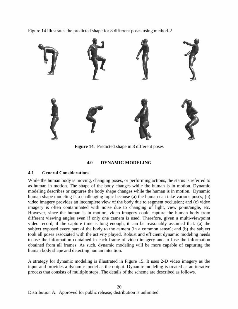
Figure 14 illustrates the predicted shape for 8 different poses using method-2.

Figure 14. Predicted shape in 8 different poses

4.0 DYNAMIC MODELING

4.1 General Considerations

While the human body is moving, changing poses, or performing actions, the status is referred to

as human in motion. The shape of the body changes while the human is in motion. Dynamic

modeling describes or captures the body shape changes while the human is in motion. Dynamic

human shape modeling is a challenging topic because (a) the human can take various poses; (b)

video imagery provides an incomplete view of the body due to segment occlusion; and (c) video

imagery is often contaminated with noise due to changing of light, view point/angle, etc.

However, since the human is in motion, video imagery could capture the human body from

different viewing angles even if only one camera is used. Therefore, given a multi-viewpoint

video record, if the capture time is long enough, it can be reasonably assumed that: (a) the

subject exposed every part of the body to the camera (in a common sense); and (b) the subject

took all poses associated with the activity played. Robust and efficient dynamic modeling needs

to use the information contained in each frame of video imagery and to fuse the information

obtained from all frames. As such, dynamic modeling will be more capable of capturing the

human body shape and detecting human intention.

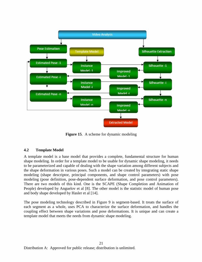
A strategy for dynamic modeling is illustrated in Figure 15. It uses 2-D video imagery as the

input and provides a dynamic model as the output. Dynamic modeling is treated as an iterative

process that consists of multiple steps. The details of the scheme are described as follows.

21


Figure 15. A scheme for dynamic modeling

4.2 Template Model

A template model is a base model that provides a complete, fundamental structure for human

shape modeling. In order for a template model to be usable for dynamic shape modeling, it needs

to be parameterized and capable of dealing with the shape variation among different subjects and

the shape deformation in various poses. Such a model can be created by integrating static shape

modeling (shape descriptor, principal components, and shape control parameters) with pose

modeling (pose definition, pose-dependent surface deformation, and pose control parameters).

There are two models of this kind. One is the SCAPE (Shape Completion and Animation of

People) developed by Anguelov et al [8]. The other model is the statistic model of human pose

and body shape developed by Hasler et al [14].

The pose modeling technology described in Figure 9 is segment-based. It treats the surface of

each segment as a whole, uses PCA to characterize the surface deformation, and handles the

coupling effect between shape variations and pose deformations. It is unique and can create a

template model that meets the needs from dynamic shape modeling.

22


4.3 Instance Model

An instance model is the model constructed from the template model for the subject in a

particular pose (corresponding to a particular video frame). In order to generate the first instance

model, semantic shape reconstruction scheme (Figure 8) can be implemented to use any shape

information available (from gender, race, and age to size parameters). If none of these data are

provided, a generic shape model (a 50th

% male, for example) can be generated. For the instance

models in the subsequent poses (frames), the shape information comes from the optimization

(fitting) in the previous step. The pose information for each instance model in the first iteration is

provided by video analysis. In the subsequent iterations, the pose information for each instance

model is provided by the fitted model in the previous iteration at the same frame.

4.4 Model fitting

Each instance model provides a set of initial values for the control parameters of the model,

which are usually not good enough for the description of the ground truth of the shape. The

estimation of the parameters of the true model is done by fitting the projection of the instance

model to the silhouette extracted from video imagery. The problem of model fitting can be

formulated as an optimization problem.

Denote

TTT

m}{ αβp , (30)

as the vector of model parameters, where T

n}...{

21β , (31)

as the control parameters for the shape variation and T

m

T }...{21α , (32)

as the control parameters for the pose-dependent surface deformation. Then, from the template

model,

)(m

S pS , (33)

which is a shape descriptor vector and represents the shape model corresponding to control

parameters m

p .

For a given camera view, a foreground silhouetteIF , which extracts the subject from

background, is computed using standard background subtraction methods. The hypothesized

shape model is projected onto the plane which is defined byIF :

),( γSPF M , (34)

where γ is the parameter related to camera view which may or may not be known. The

projection MF can be considered as the estimated silhouette in the same frame. The extraction of

a dynamic model from video imagery can be conducted by fitting MF to

IF for a sequence of

image frames where the method proposed by Balan et al [15] can be used. The cost function is a

measure of similarity between two these silhouettes. For a given camera view, a foreground

silhouette IF is computed using standard background subtraction methods. This is then

compared with the model silhouetteMF . The pixels in non-overlapping regions in one silhouette

23


are penalized by the shortest distance to the other silhouette [16] and vice-versa. To do so, a

Chamfer distance map [17] is computed for each silhouette, MC for the hypothesized model and

IC for the image silhouette. This process is illustrated in Figure 16. The predicted silhouette

should not exceed the image foreground silhouette (therefore minimizingIM CF ), while at the

same time trying to explain as much of it as possible (thus minimizingMICF ). Both constraints

are combined into a cost function that sums the errors over all image pixels px :

Figure 16. Cost function

(a) original image I (top) and hypothesized mesh M (bottom); (b) image foreground silhouetteIF and mesh silhouette

MF , with 1 for foreground and 0 for background; (c) Chamfer distance

maps IC and

MC , which are 0 inside the silhouette; the opposing silhouette is overlaid

transparently; (d) contour maps for visualizing the distance maps; (e) per pixel silhouette

distance from MF to

IF given by px

I

px

M

pxCF (top), and from

IF toMF given

px

M

px

I

pxCF

(bottom).

px

M

px

I

px

I

px

M

pxCFCF

pxf ))1((

1)( p , (35)

where T

γ}{ppT

m , (36)

including the control parameters of the model and the parameters related to camera view, and

weighs the first term more heavily because the image silhouettes are usually wider due to the

24


effects of clothing. When multiple views are available, the total cost is taken to be the average of

the costs for the individual views.

Now, model fitting can be formulated as an optimization as follows:

UL

f

ppp

p

p

:sConstraint

})(Min{ :function objective

:iablesDesign var

, (37)

where L

p and U

p are lower and upper bounds on the design variables, respectively. The problem

of Eq. (33) is nonlinear. While various methods are available for solving Eq. (37), local minima

and non-convergence are expected to be common problems.

4.5 Iteration

Usually, the information contained in one frame is not enough to extract a decent model. In

other words, model fitting in one pose (frame) will not be able to provide good estimates of all

parameters. Local minima and non-convergence may lead to the failure of the optimization at a

particular frame. Therefore, an iterative procedure was devised to use the information contained

in a sequence of frames and to improve the model fitting (parameter estimation) progressively.

As shown in Figure 15, the model fitting is performed on a sequence of frames. Not all the

images in consecutive frames will be used in the model fitting. Only those that can provide a

sound estimation of pose and are sufficiently distinct from the previous ones will be used for the

model fitting. After creating an initial instance model, the estimated model parameters at step i

will be used to create the instance model for step i+1, in combination with the pose estimation at

step i+1. If the optimization at step i fails, the estimated model parameters from step i-1 will be

used to create the instance model for step i+1, with a certain perturbation incorporated. After all

the frames in the sequence have been run through, the estimated model parameters at the last step

will be used to create the instance model for the first step in the new run. The iteration will repeat

until certain tolerances for errors are met.

4.6 Computation Efficiency

It was shown that dynamic model fitting is a time consuming process [15]. As an iterative

procedure is to be used to improve model fitting, computational efficiency becomes more

important. In particular, the optimization used in model fitting will incur extensive computation

as numerous times of 3-D mesh reconstruction and 3-D model projection will be called. In order

to perform dynamic modeling in real-time or in nearly real-time, the following measures will be

taken to increase computational efficiency.

Using graphics hardware for the projection of 3-D meshes and the computation of the cost

function;

Implementing parallel computing using CUDA, a parallel computing architecture from

NVIDIA. As a general purpose parallel computing architecture, CUDA leverages the parallel

computational engine in graphics processing units (GPUs) to solve many complex

computational problems in a fraction of the time required on a CPU. It includes the CUDA

Instruction Set Architecture (ISA) and the parallel computational engine in the GPU. To

program to the CUDA architecture, developers can use C, FORTRAN, C++, and MATLAB.

http://en.wikipedia.org/wiki/NVIDIA

25


Implementing distributed computing to exploit the computing power of a multi-node cluster

workstation. Distributed computing often requires parallel schemes. This will greatly

enhance our computational capability. In order to attain the goal of real-time dynamic

modeling, the implementation of parallel, distributed computing is necessary.

5.0 REPLICATION AND ANIMATION

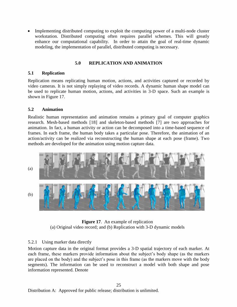
5.1 Replication

Replication means replicating human motion, actions, and activities captured or recorded by

video cameras. It is not simply replaying of video records. A dynamic human shape model can

be used to replicate human motion, actions, and activities in 3-D space. Such an example is

shown in Figure 17.

5.2 Animation

Realistic human representation and animation remains a primary goal of computer graphics

research. Mesh-based methods [18] and skeleton-based methods [7] are two approaches for

animation. In fact, a human activity or action can be decomposed into a time-based sequence of

frames. In each frame, the human body takes a particular pose. Therefore, the animation of an

action/activity can be realized via reconstructing the human shape at each pose (frame). Two

methods are developed for the animation using motion capture data.

(a)

(b)

Figure 17. An example of replication

(a) Original video record; and (b) Replication with 3-D dynamic models

5.2.1 Using marker data directly

Motion capture data in the original format provides a 3-D spatial trajectory of each marker. At

each frame, these markers provide information about the subject’s body shape (as the markers

are placed on the body) and the subject’s pose in this frame (as the markers move with the body

segments). The information can be used to reconstruct a model with both shape and pose

information represented. Denote

26


T

nznynxzyxzyxjmmmmmmmmm }...{ˆ

222111m , (38)

as the coordinate vector of the markers at frame j. We use control parameters j

mp to create a

model mesh at this frame,j

S , which is given by

)( j

mS pS

j . (39)

From this model, we can calculate the coordinates of the points corresponding to the markers,

which are denoted as j

m~ . The reconstruction of the model is to find a set of parameters j

mop

such that points j

m~ get as close to markers j

m̂ as possible. This can be formulated as an

optimization problem:

U

m

L

m

jj

j

m

ppp

mm

p

j

m

:sConstraint

ˆ~Min :function Objective

:iablesDesign var

. (40)

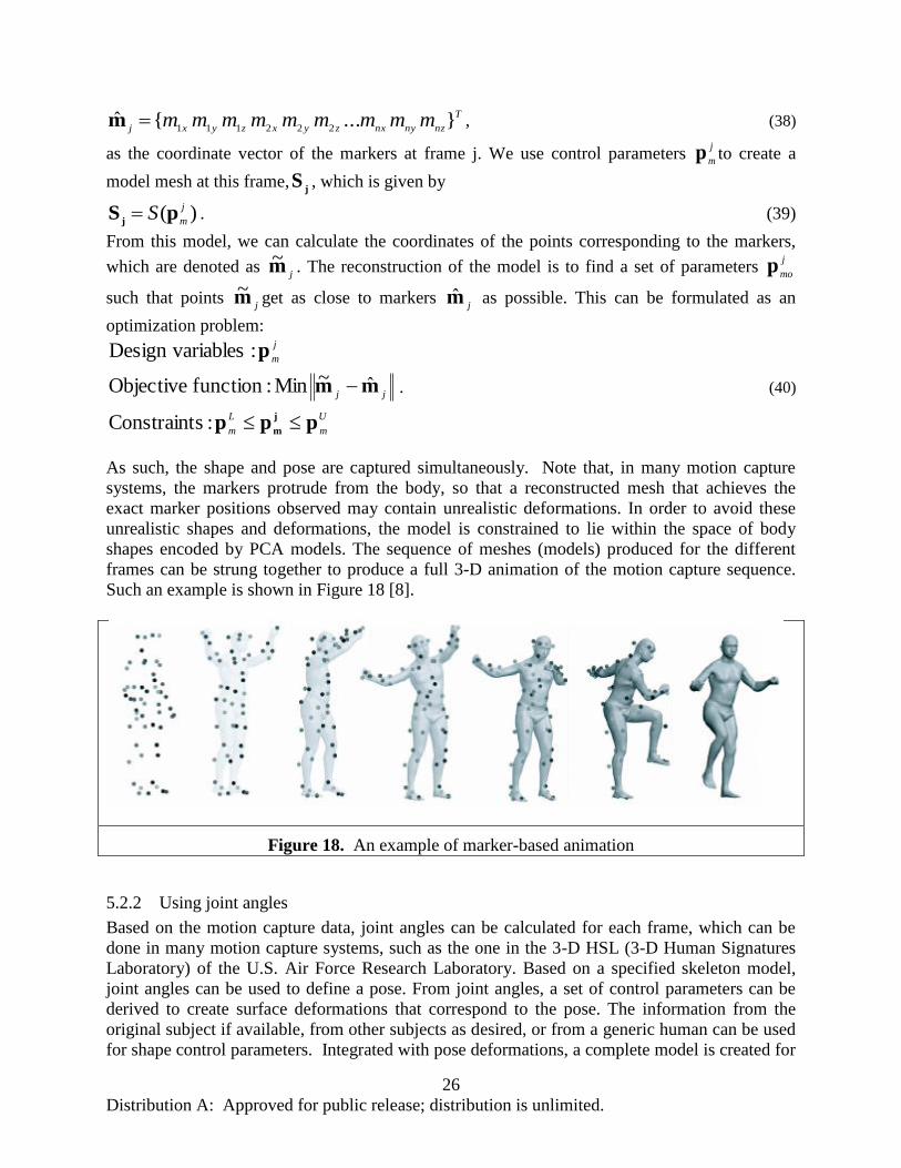
As such, the shape and pose are captured simultaneously. Note that, in many motion capture

systems, the markers protrude from the body, so that a reconstructed mesh that achieves the

exact marker positions observed may contain unrealistic deformations. In order to avoid these

unrealistic shapes and deformations, the model is constrained to lie within the space of body

shapes encoded by PCA models. The sequence of meshes (models) produced for the different

frames can be strung together to produce a full 3-D animation of the motion capture sequence.

Such an example is shown in Figure 18 [8].

Figure 18. An example of marker-based animation

5.2.2 Using joint angles

Based on the motion capture data, joint angles can be calculated for each frame, which can be

done in many motion capture systems, such as the one in the 3-D HSL (3-D Human Signatures

Laboratory) of the U.S. Air Force Research Laboratory. Based on a specified skeleton model,

joint angles can be used to define a pose. From joint angles, a set of control parameters can be

derived to create surface deformations that correspond to the pose. The information from the

original subject if available, from other subjects as desired, or from a generic human can be used

for shape control parameters. Integrated with pose deformations, a complete model is created for

27


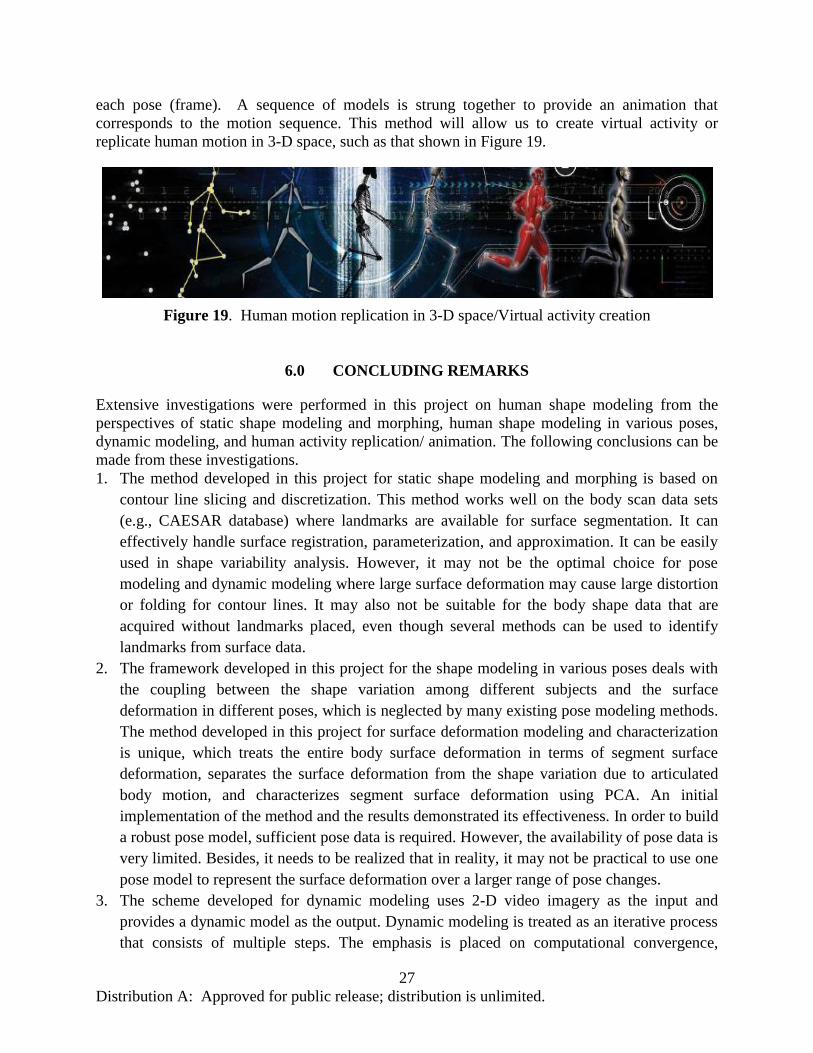
each pose (frame). A sequence of models is strung together to provide an animation that

corresponds to the motion sequence. This method will allow us to create virtual activity or

replicate human motion in 3-D space, such as that shown in Figure 19.

Figure 19. Human motion replication in 3-D space/Virtual activity creation

6.0 CONCLUDING REMARKS

Extensive investigations were performed in this project on human shape modeling from the

perspectives of static shape modeling and morphing, human shape modeling in various poses,

dynamic modeling, and human activity replication/ animation. The following conclusions can be

made from these investigations.

1. The method developed in this project for static shape modeling and morphing is based on

contour line slicing and discretization. This method works well on the body scan data sets

(e.g., CAESAR database) where landmarks are available for surface segmentation. It can

effectively handle surface registration, parameterization, and approximation. It can be easily

used in shape variability analysis. However, it may not be the optimal choice for pose

modeling and dynamic modeling where large surface deformation may cause large distortion

or folding for contour lines. It may also not be suitable for the body shape data that are

acquired without landmarks placed, even though several methods can be used to identify

landmarks from surface data.

2. The framework developed in this project for the shape modeling in various poses deals with

the coupling between the shape variation among different subjects and the surface

deformation in different poses, which is neglected by many existing pose modeling methods.

The method developed in this project for surface deformation modeling and characterization

is unique, which treats the entire body surface deformation in terms of segment surface

deformation, separates the surface deformation from the shape variation due to articulated

body motion, and characterizes segment surface deformation using PCA. An initial

implementation of the method and the results demonstrated its effectiveness. In order to build

a robust pose model, sufficient pose data is required. However, the availability of pose data is

very limited. Besides, it needs to be realized that in reality, it may not be practical to use one

pose model to represent the surface deformation over a larger range of pose changes.

3. The scheme developed for dynamic modeling uses 2-D video imagery as the input and

provides a dynamic model as the output. Dynamic modeling is treated as an iterative process

that consists of multiple steps. The emphasis is placed on computational convergence,

28


efficiency, and robustness, the common problems for dynamic modeling. For the dynamic

modeling, the template model is important. It has to be parameterized and able to handle

shape variation and surface deformation. While the models of such kind have been

investigated and developed [8, 14], they are not available for public use. Implementing their

methods and developing a customized dynamic template model is still a great challenge.

4. Based on a dynamic model, human activity can be replicated or created using marker data or

joint angles. One important application of human activity replication and animation is M&S

(modeling and simulation) based training. The high bio-fidelity provided by dynamic human

modeling will enhance the representation and display of bio-signatures that are unique and

critical to a particular mission and can thus improve the trainee’s cognitive performance in

real-world missions.

This project attained its goal to develop concepts and methodologies for dynamic human shape

modeling. While major objectives have been achieved, significant efforts are still needed to

address remaining issues. In particular, human shape data in various poses need to be collected

for pose modeling, and the methods and algorithms developed need to be implemented on the

test data sets. The end goal of human shape modeling is to develop a software tool or system that

can be used to extract a dynamic model from 2-D video imagery or 3-D sensor data. To achieve

that goal, major efforts are needed on technology implementation, software development, and

system integration.

7.0 REFERENCES

1. Zhiqing Cheng and Kathleen Robinette, Static and Dynamic Human Shape Modeling – A

Review of the Literature and State of the Art, Technical report, Air Force Research

Laboratory, AFRL-RH-WP-TR-2010-0023, 2010.

2. Dennis Burnsides, INTEGRATE 2.8: A New Generation Three-Dimensional Visualization,

Analysis, and Manipulation Utility, Technical report, Air Force Research Laboratory, AFRL-

HE-WP-TR-2004-0169, 2004.

3. Kathleen Robinette et al., Civilian American and European Surface Anthropometry Resource

(CAESAR), Final report, Air Force Research Laboratory, 2002.

4. Allen, B., Curless, B., and Popvic, Z. (2003). “The space of human body shapes:

reconstruction and parameterization from range scans,” in ACM SIGGRAPH 2003, 27-31

July 2003, San Diego, CA, USA.

5. Ben Azouz, B.Z., Rioux, M., Shu, C., and Lepage, R. (2005a). “Characterizing Human Shape

Variation Using 3-D Anthropometric Data,” International Journal of Computer Graphics,

volume 22, number 5, pp. 302-314, 2005.

6. Hohenstein, Uniform Body Representation, Workpackage Input, E-Tailor project, IST-1999-

10549.

7. H.Seo, N. Magnenat-Thalmann, An example-based approach to human body manipulation,

Graphical Models 66 (2004) 1-23.

29


8. Anguelov, D., Srinivasan, P., Koller, D., Thrun, S., Rodgers, J. and Davis, J. (2005b).

"SCAPE: Shape Completion and Animation of People." ACM Transactions on Graphics

(SIGGRAPH) 24(3).

9. Davis, J., Marschner, S., Garr, M., and Levoy, M. (2002). “Filling Holes in Complex

Surfaces Using Volumetric Diffusion”, in: Symposium on 3-D Data Processing,

Visualization, and Transmission.

10. Chui, H. and Rangarajan, A. (2000). “A new point matching algorithm for non-rigid

registration”, in: Proceedings of the Conference on Computer Vision and Pattern Recognition

(CVPR)

11. Rusinkiewicz, S. and Levoy, M. (2001). “Efficient variants of the ICP algorithm”, in: Proc.

3DIM, Quebec City, Canada, 2001. IEEEComputer Society.

12. Anguelov, D., Koller, D., Pang, H.C., Srinivasan, P., and Thrun, S. (2004). “Recovering

Articulated Object Models from 3D Range Data,” in Proceedings of the 20th conference on

Uncertainty in artificial intelligence, Pages: 18 – 26, 2004.

13. Anguelov, D., Srinivasan, P., Pang, H.C., Koller, D., Thrun, S., and Davis, J. (2005a). “The

correlated correspondence algorithm for unsupervised registration of nonrigid surfaces,”

Advances in Neural Information Processing Systems 17, 33-40.

14. Hasler, N. Stoll, C., Sunkel, M., Rosenhahn, B., and Seidel H.-P., A Statistical Model of

Human Pose and Body Shape, EuroGraphics, Vol 28 No. 2, 2009.

15. Balan, A., Sigal, L., Black, M., Davis, J., and Haussecker, H.: Detailed Human Shape and

Pose from Images. In: IEEE Conf. on Comp. Vision and Pattern Recognition (CVPR) (2007).

16. C. Sminchisescu and A. Telea. Human pose estimation from silhouettes a consistent

approach using distance level sets. WSCG Int. Conf. Computer Graphics, Visualization and

Computer Vision, 2002.

17. C. Stauffer and W. Grimson, “Adaptive background mixture models for real-time tracking,”

Proceedings of the IEEE Computer Society Conference on Computer Vision and Pattern

Recognition, Vol. 2, pp. 246-252, (1999)

18. Aguiar, E., Zayer, R., Theobalt, C., Magnor, M., Seidel, H.P.: A Framework for Natural

Animation of Digitized Models. In MPI-I-2006-4-003 (2006).

30


8.0 GLOSSARY/ACRONYMS

2-D Two-Dimensional

3-D Three-Dimensional

CAESAR Civilian American and European Surface Anthropometry Resource

CPU Central Processing Unit

GPU Graphics Processing Unit

GRBF Gaussian Radial Basis Function

HSL Human Signatures Laboratory

IPCA Incremental Principal Component Analysis

ISA Instruction Set Architecture

M&S Modeling and Simulation

PCA Principal Component Analysis

PC Principal Component

SCAPE Shape Completion and Animation of PEople

Date post:	16-Jun-2018
Category:	Documents
Upload:	lynhan
View:	241 times
Download:	0 times

Static and Dynamic Human Shape Modeling … Static and Dynamic Human Shape Modeling – Concept...

Documents