Static Scheduling for Embedded Systems Luciano Lavagno University of Udine and Cadence Berkeley Labs Joint work with: Jordi Cortadella, Alex Kondratyev, Marc Massot, Sandra Moral, Claudio Passerone, Alberto Sangiovanni-Vincentelli, Marco Sgroi, Yosinori Watanabe
Transcript
Static Schedulingfor Embedded Systems
Luciano LavagnoUniversity of Udine and Cadence Berkeley Labs
Joint work with:
Jordi Cortadella, Alex Kondratyev, Marc Massot,Sandra Moral, Claudio Passerone,Alberto Sangiovanni-Vincentelli, Marco Sgroi,Yosinori Watanabe
Outline
• Motivation
• Static Scheduling of dataflow networks– schedulability
– code and data size optimization
• Quasi-Static Scheduling of processnetworks using Petri nets– Free Choice nets
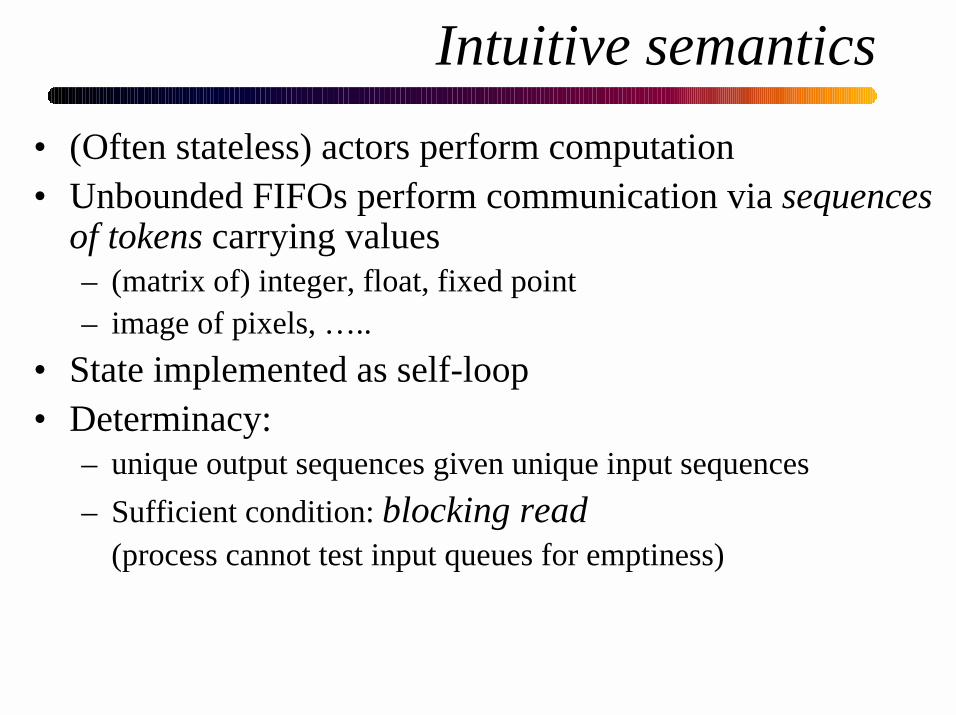
• (Often stateless) actors perform computation• Unbounded FIFOs perform communication via sequences
of tokens carrying values– (matrix of) integer, float, fixed point– image of pixels, …..
• State implemented as self-loop• Determinacy:
– unique output sequences given unique input sequences
– Sufficient condition: blocking read(process cannot test input queues for emptiness)
Intuitive semantics
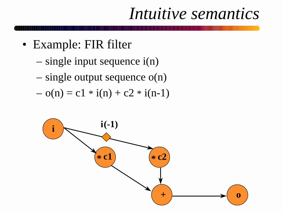
• Example: FIR filter– single input sequence i(n)
– single output sequence o(n)
– o(n) = c1 * i(n) + c2 * i(n-1)
* c1
+ o
i
* c2
i(-1)
Examples of Dataflow actors
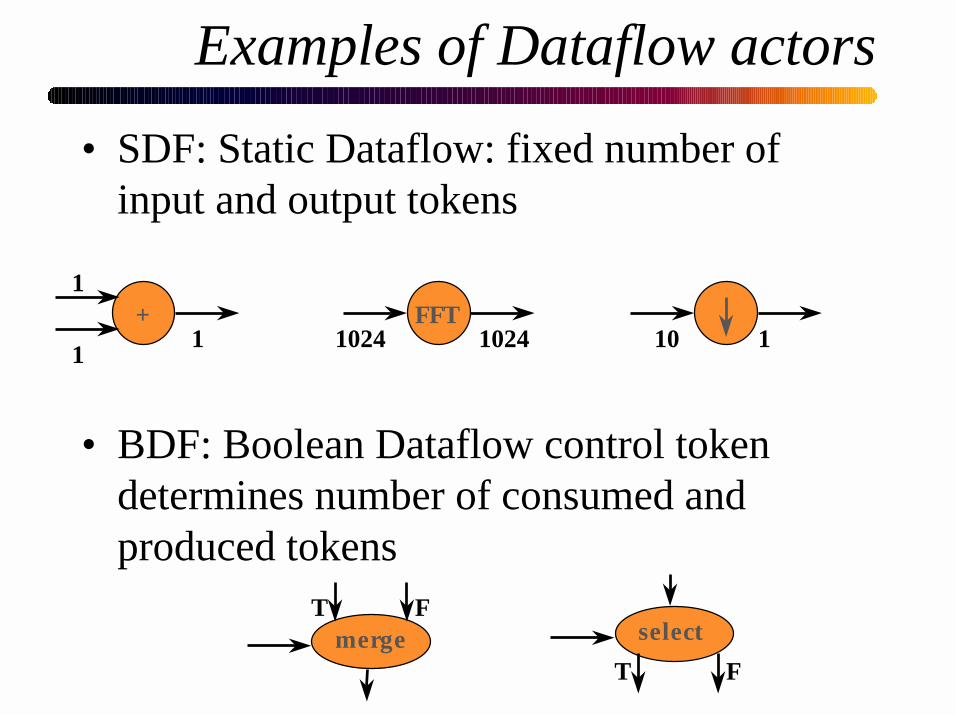
• SDF: Static Dataflow: fixed number ofinput and output tokens
• BDF: Boolean Dataflow control tokendetermines number of consumed andproduced tokens
+1
11
FFT1024 1024 10 1
merge selectT F
FT
Outline
• Motivation
• Static Scheduling of dataflow networks– schedulability
– code and data size optimization
• Quasi-Static Scheduling of processnetworks using Petri nets– Free Choice nets
– Non-Free-Choice nets
• Conclusions
Static scheduling of DF
• Key property of DF networks: output sequences do notdepend on firing sequence of actors
• SDF networks can be statically scheduled at compile-time– execute an actor when it is known to be fireable– no overhead due to sequencing of concurrency– static buffer sizing
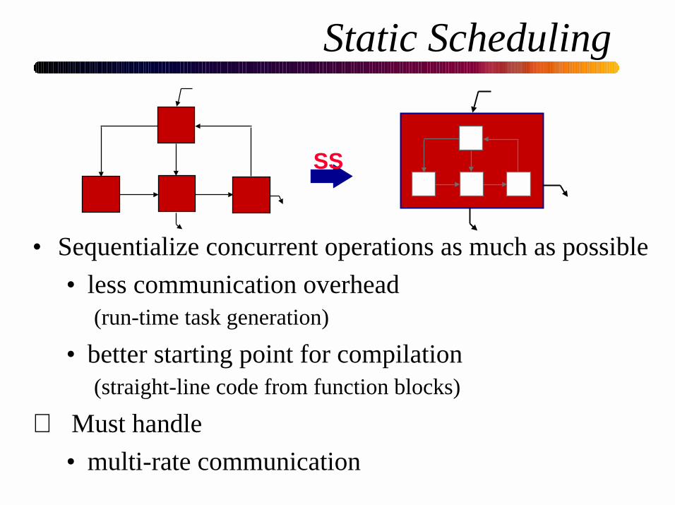
• Sequentialize concurrent operations as much as possible
• less communication overhead (run-time task generation)
• better starting point for compilation (straight-line code from function blocks)
⇒ Must handle
• multi-rate communication
SS
Static scheduling of SDF
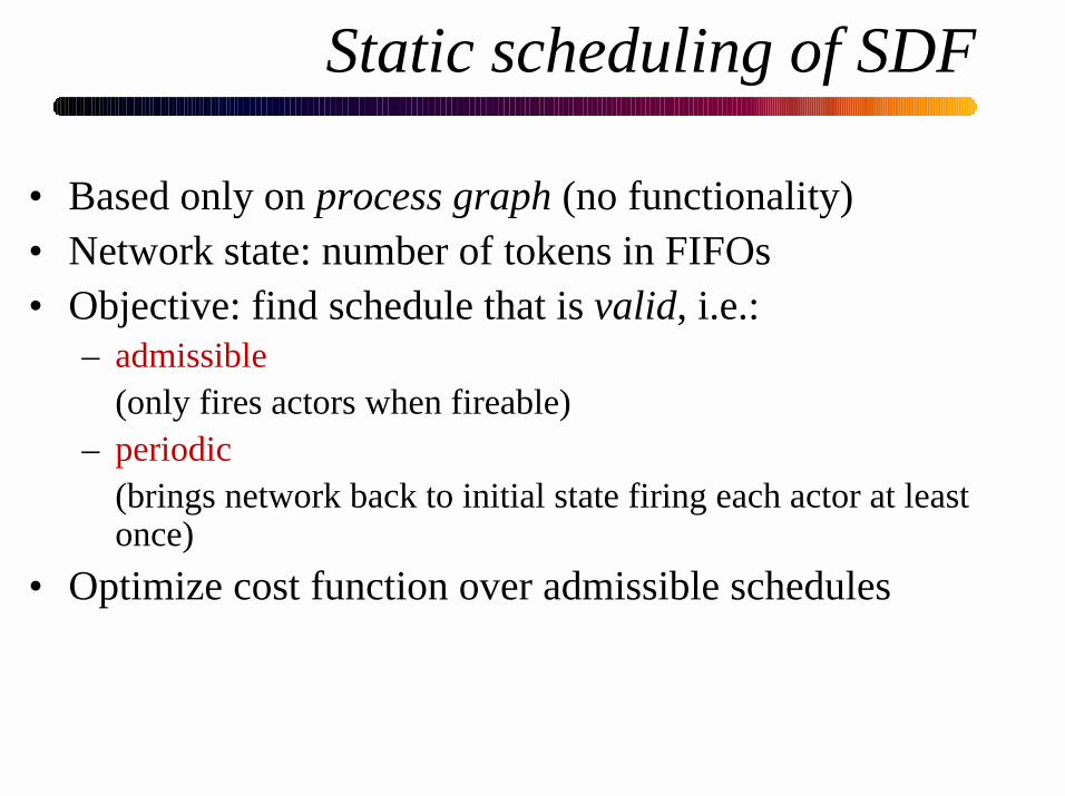
• Based only on process graph (no functionality)• Network state: number of tokens in FIFOs• Objective: find schedule that is valid, i.e.:
– admissible(only fires actors when fireable)
– periodic(brings network back to initial state firing each actor at leastonce)
• Optimize cost function over admissible schedules
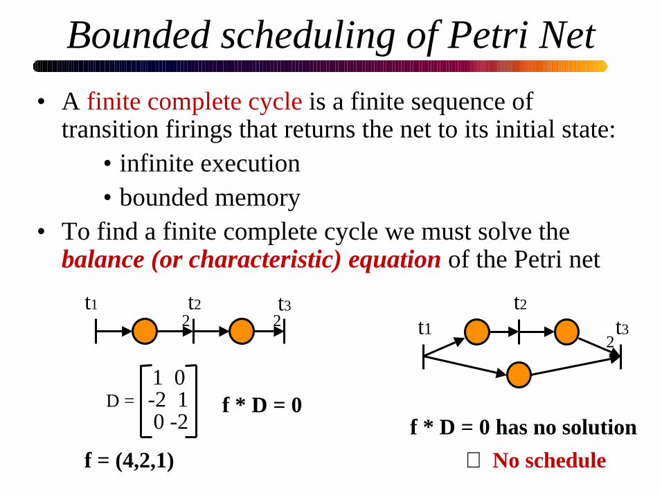
Balance equations
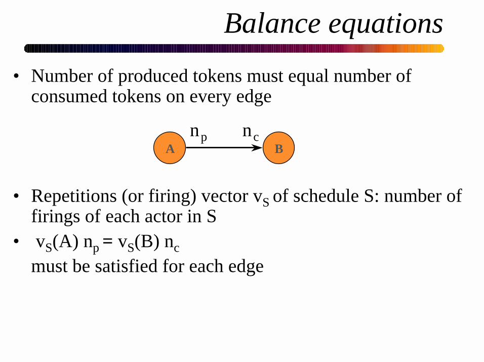
• Number of produced tokens must equal number ofconsumed tokens on every edge
• Repetitions (or firing) vector vS of schedule S: number offirings of each actor in S
• vS(A) np = vS(B) nc
must be satisfied for each edge
np ncA B
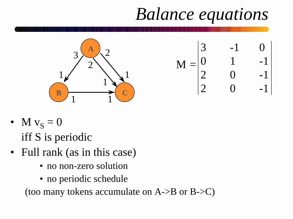
Balance equations
B C
A3
1
1
1
22
11
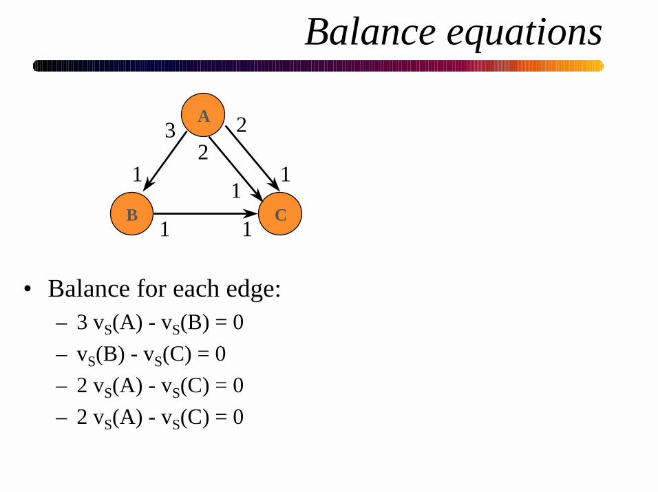
• Balance for each edge:– 3 vS(A) - vS(B) = 0
– vS(B) - vS(C) = 0
– 2 vS(A) - vS(C) = 0
– 2 vS(A) - vS(C) = 0
Balance equations
• M vS = 0iff S is periodic
• Full rank (as in this case)• no non-zero solution• no periodic schedule
(too many tokens accumulate on A->B or B->C)
3 -1 00 1 -12 0 -12 0 -1
M =
B C
A3
1
1
1
22
11
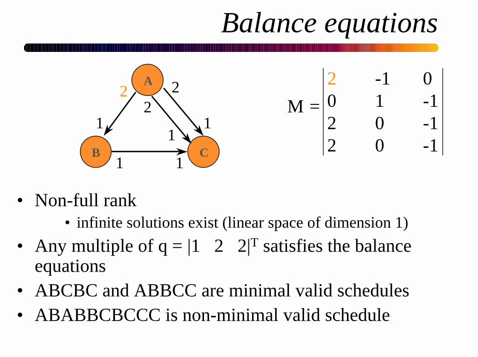
Balance equations
• Non-full rank• infinite solutions exist (linear space of dimension 1)
• Any multiple of q = |1 2 2|T satisfies the balanceequations
• ABCBC and ABBCC are minimal valid schedules• ABABBCBCCC is non-minimal valid schedule
2 -1 00 1 -12 0 -12 0 -1
M =
B C
A2
1
1
1
22
11
Static SDF scheduling
• Main SDF scheduling theorem (Lee ‘86):– A connected SDF graph with n actors has a
periodic schedule iff its topology matrix M hasrank n-1
– If M has rank n-1 then there exists a uniquesmallest integer solution q to
M q = 0
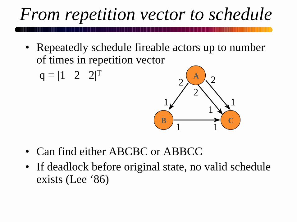
From repetition vector to schedule
• Repeatedly schedule fireable actors up to numberof times in repetition vector q = |1 2 2|T
• Can find either ABCBC or ABBCC• If deadlock before original state, no valid schedule
exists (Lee ‘86)
B C
A2
1
1
1
22
11
From schedule to implementation
• Static scheduling used for:– behavioral simulation of DF code generation
for DSP– HW synthesis (Cathedral, Lager, …)
• Issues in code generation– execution speed (pipelining, vectorization)– code size minimization– data memory size minimization (allocation to
FIFOs)– processor or functional unit allocation
Outline
• Motivation
• Static Scheduling of dataflow networks– schedulability
– code and data size optimization
• Quasi-Static Scheduling of processnetworks using Petri nets– Free Choice nets
– Non-Free-Choice nets
• Conclusions
Compilation optimization
• Assumption: code stitching(chaining custom code for each actor)
• More efficient than C compiler for DSP
• Comparable to hand-coding in some cases
• Explicit parallelism, no artificial controldependencies
• Main problem: memory and processor/FUallocation depends on scheduling, and vice-versa
Code size minimization
• Assumptions (based on DSP architecture):– subroutine calls expensive
– fixed iteration loops are cheap
(“zero-overhead loops”)
• Global optimum: single appearance schedulee.g. ABCBC -> A (2BC), ABBCC -> A (2B) (2C)
• may or may not exist for an SDF graph…
• buffer minimization relative to single appearanceschedules
(Bhattacharyya ‘94, Lauwereins ‘96, Murthy ‘97)
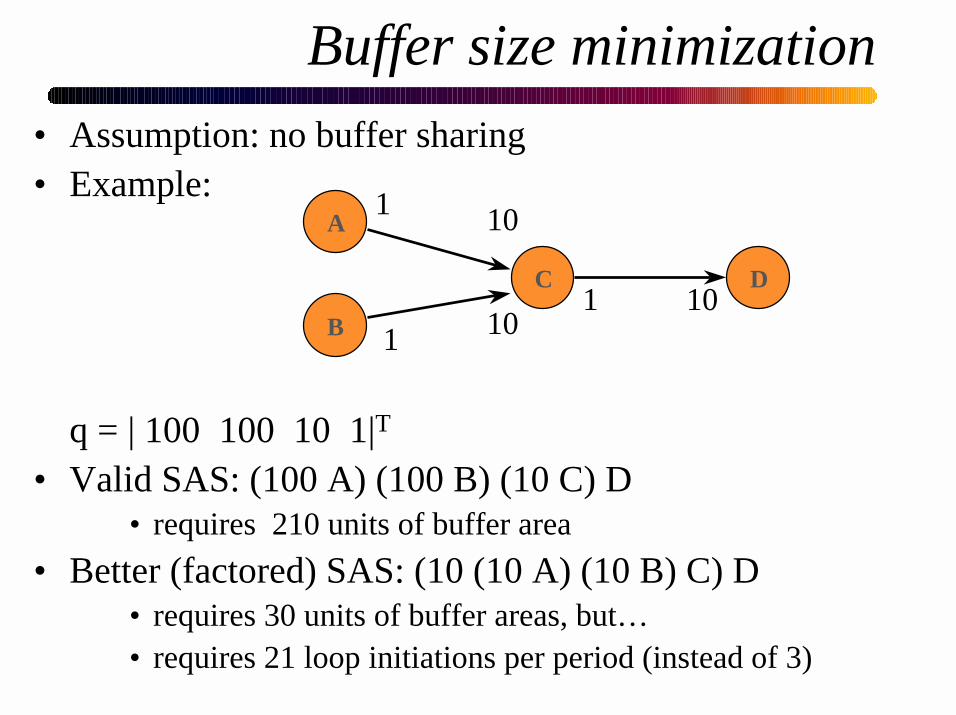
• Assumption: no buffer sharing• Example:
q = | 100 100 10 1|T
• Valid SAS: (100 A) (100 B) (10 C) D• requires 210 units of buffer area
• Better (factored) SAS: (10 (10 A) (10 B) C) D• requires 30 units of buffer areas, but…• requires 21 loop initiations per period (instead of 3)
Buffer size minimization
C D1 10
A
B 10
10
1
1
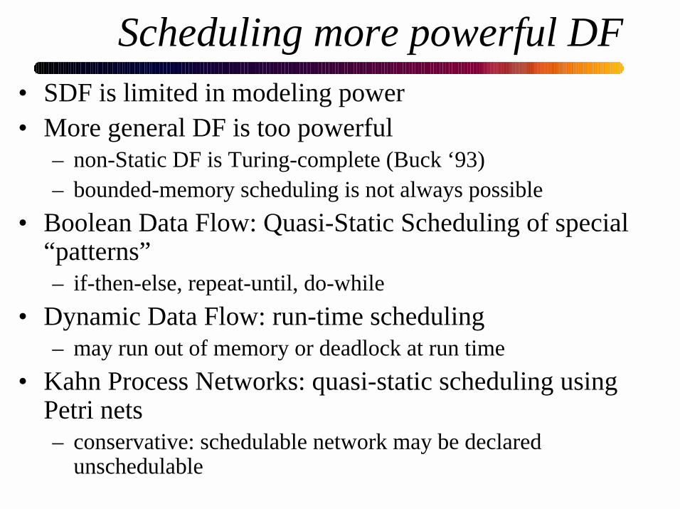
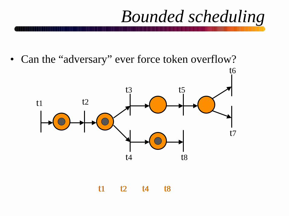
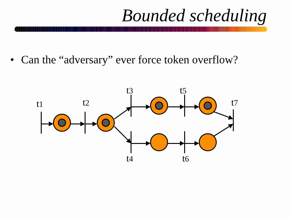
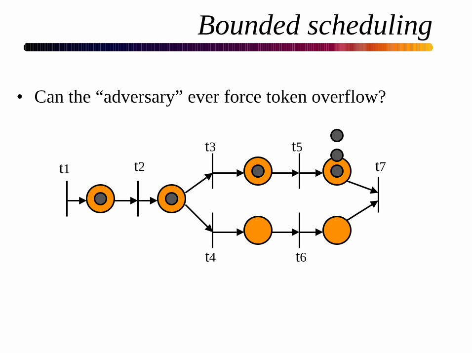
Scheduling more powerful DF• SDF is limited in modeling power• More general DF is too powerful
– non-Static DF is Turing-complete (Buck ‘93)– bounded-memory scheduling is not always possible
• Boolean Data Flow: Quasi-Static Scheduling of special“patterns”– if-then-else, repeat-until, do-while
• Dynamic Data Flow: run-time scheduling– may run out of memory or deadlock at run time
• Kahn Process Networks: quasi-static scheduling usingPetri nets– conservative: schedulable network may be declared
unschedulable
Outline
• Motivation
• Static Scheduling of dataflow networks– schedulability
– code and data size optimization
• Quasi-Static Scheduling of processnetworks using Petri nets– Free Choice nets
– Non-Free-Choice nets
• Conclusions
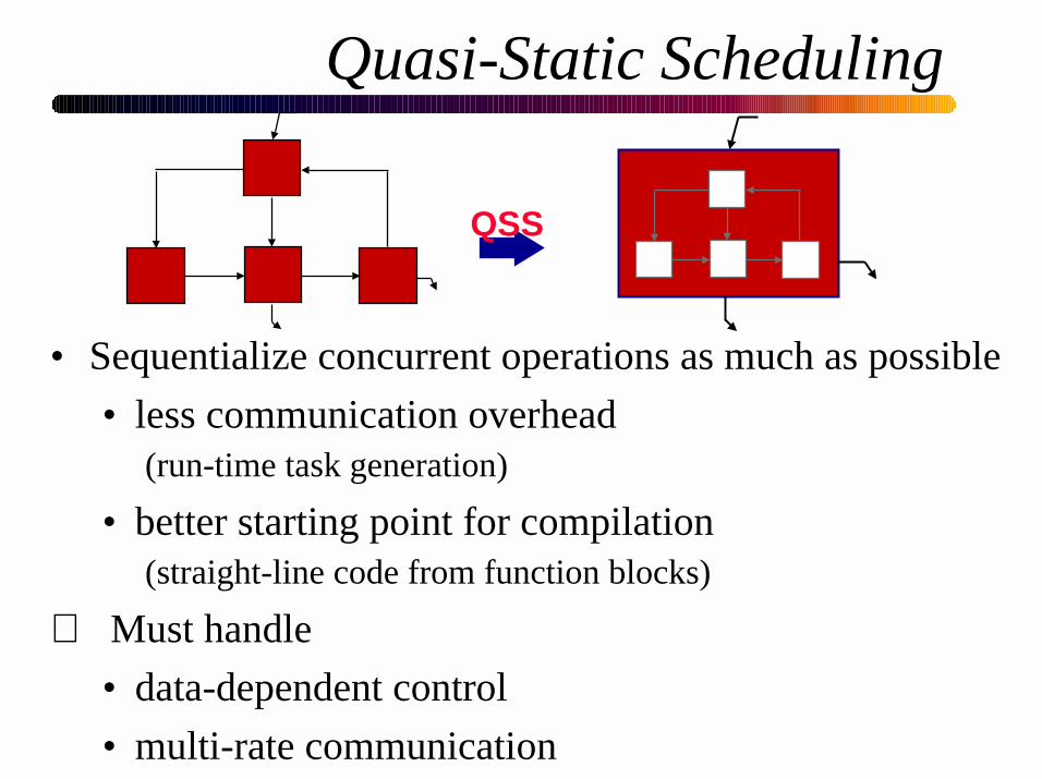
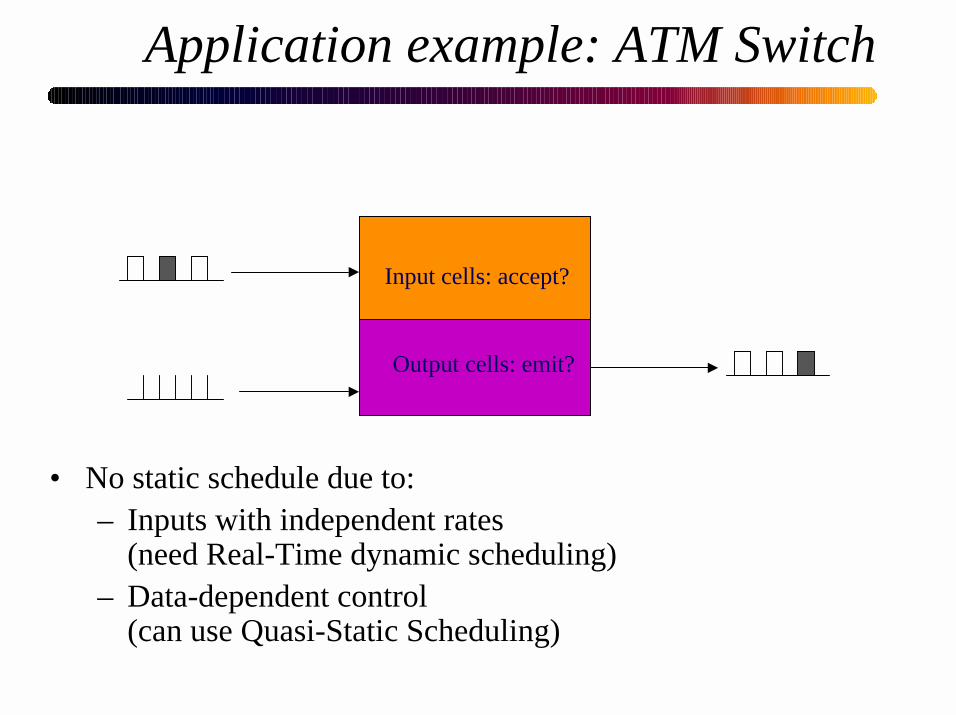
Quasi-Static Scheduling
• Sequentialize concurrent operations as much as possible
• less communication overhead (run-time task generation)
• better starting point for compilation (straight-line code from function blocks)
⇒ Must handle
• data-dependent control
• multi-rate communication
QSS
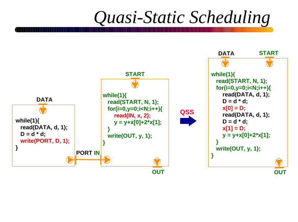
Quasi-Static Scheduling
QSS
OUT
START
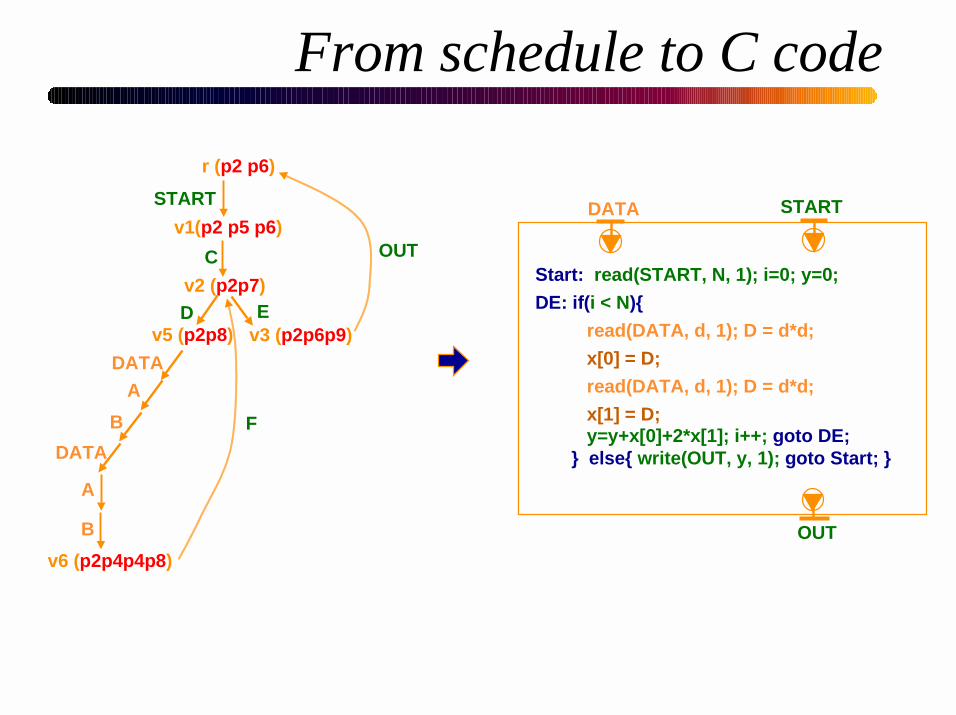
while(1){ read(START, N, 1); for(i=0,y=0;i<N;i++){ read(DATA, d, 1); D = d * d; x[0] = D; read(DATA, d, 1); D = d * d; x[1] = D; y = y+x[0]+2*x[1]; } write(OUT, y, 1);}
DATA
DATA
PORT IN
while(1){ read(START, N, 1); for(i=0,y=0;i<N;i++){ read(IN, x, 2); y = y+x[0]+2*x[1]; } write(OUT, y, 1);}
while(1){ read(DATA, d, 1); D = d * d; write(PORT, D, 1);}
START
OUT
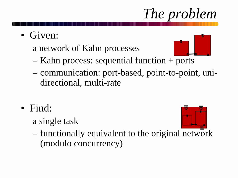
The problem
• Given:a network of Kahn processes– Kahn process: sequential function + ports– communication: port-based, point-to-point, uni-
directional, multi-rate
• Find:a single task– functionally equivalent to the original network
(modulo concurrency)
The scheduling procedure
1. Specify a network of processes– process: C + communication
operations– netlist: connection between ports
2. Translate to the computationalmodel: Petri nets
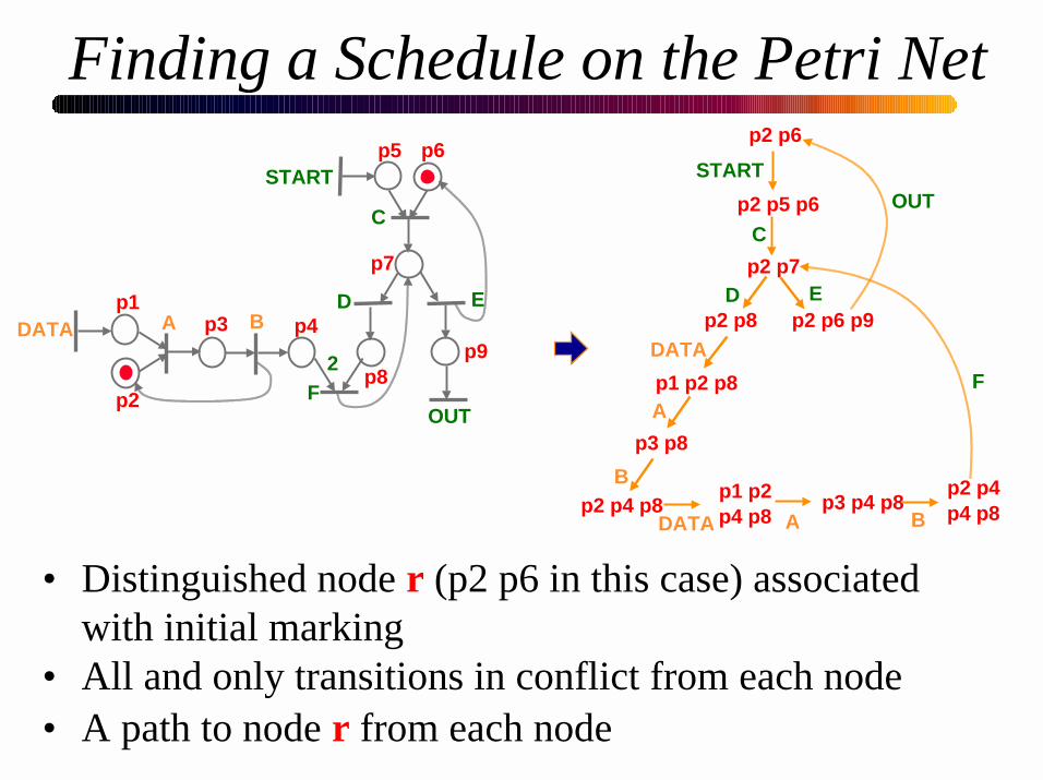
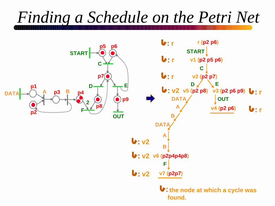
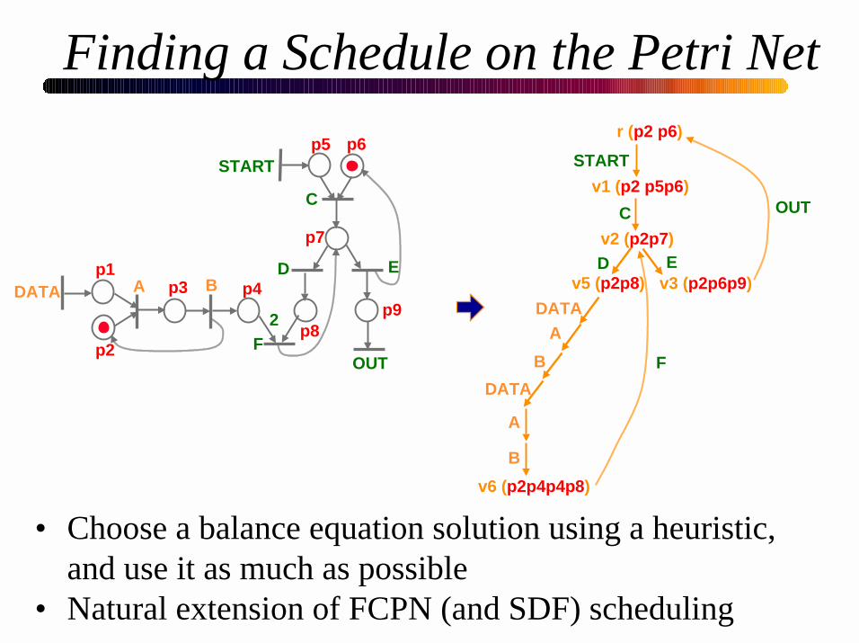
3. Find a “schedule” on the Petri net
4. Translate the schedule to a task
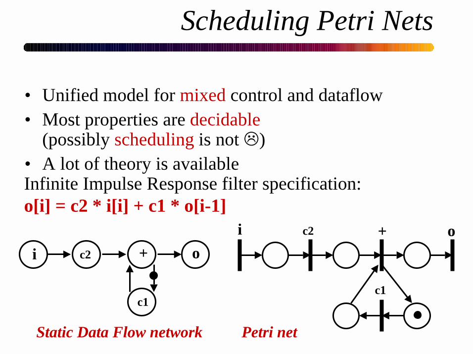
Scheduling Petri Nets
• Unified model for mixed control and dataflow• Most properties are decidable
(possibly scheduling is not !)• A lot of theory is available
T-invariant: a basis of the linear system A x = 0A[i, j]: # of tokens produced to the i-th place
by the j-th transition. DATA A B START C D E F OUT [ 0 0 0 1 1 0 1 0 1 ] [ 2 2 2 0 0 1 0 1 0 ]
– Choose a T-invariant using a heuristic, and use itas much as possible.
OUT
DATA A B
2
START
C
D E
F
p1
p2
p3 p4
p5 p6
p7
p8p9
START
OUT
r (p2 p6)
v1 (p2p5p6)
C v2 (p2 p7)
D E v3 (p2p6p9)
T-invariants:
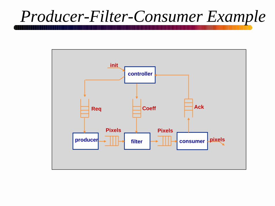
Producer-Filter-Consumer Example
controller
filterproducer consumer
init
Req AckCoeff
Pixels Pixels
pixels
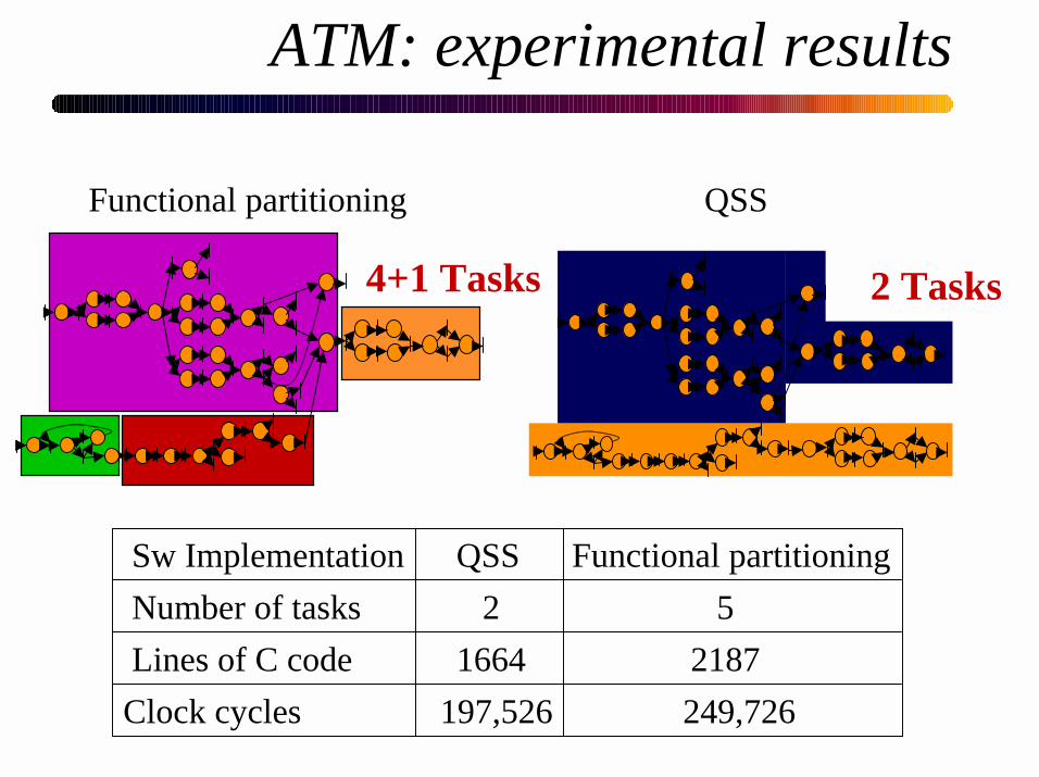
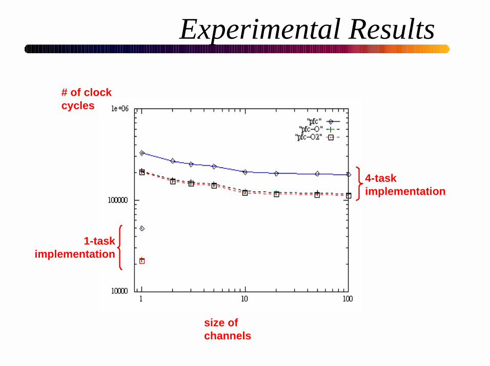
Experimental Results
# of clockcycles
size ofchannels
4-taskimplementation
1-taskimplementation
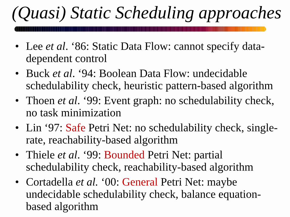
(Quasi) Static Scheduling approaches
• Lee et al. ‘86: Static Data Flow: cannot specify data-dependent control
• Buck et al. ‘94: Boolean Data Flow: undecidableschedulability check, heuristic pattern-based algorithm
• Thoen et al. ‘99: Event graph: no schedulability check,no task minimization
• Lin ‘97: Safe Petri Net: no schedulability check, single-rate, reachability-based algorithm
• Thiele et al. ‘99: Bounded Petri Net: partialschedulability check, reachability-based algorithm
• Cortadella et al. ‘00: General Petri Net: maybeundecidable schedulability check, balance equation-based algorithm
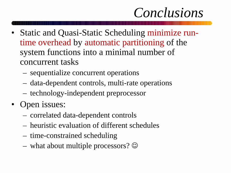
Conclusions• Static and Quasi-Static Scheduling minimize run-
time overhead by automatic partitioning of thesystem functions into a minimal number ofconcurrent tasks– sequentialize concurrent operations– data-dependent controls, multi-rate operations– technology-independent preprocessor
• Open issues:– correlated data-dependent controls– heuristic evaluation of different schedules– time-constrained scheduling– what about multiple processors? ☺