Stationary localized modes in the quintic nonlinear ... · G. L. Alﬁmov 1, V. V. Konotop2 and P....

Stationary localized modes in thequintic nonlinear Schrodinger

equation with a periodic potential

G. L. Alfimov 1, V. V. Konotop2 and P. Pacciani2

1 Moscow Institute of Electronic Engineering, Zelenograd, Moscow, 124498,

Russia2 Centro de Fısica Teorica e Computacional and Departamento de Fısica,

Faculdade de Ciencias, Universidade de Lisboa, Lisbon

Portugal

arXiv.nlin.PS/0605035

Stationary localized modes in the quintic nonlinear Schrodinger equation with a periodic potential – p.1/29

Outline


Outline• The model and its physical applications



• Analytical Results




• Numerical Results




- Sufficient conditions for collapse

- Lower bound for the number of particles

- Asymptotic behaviour of the solutions









- Behaviour of the number of particles vs frequency

- Dynamics of solutions








- Behaviour of the number of particles vs frequency

- Dynamics of solutions

• Conclusions


ModelThe Quintic Nonlinear Schrödinger Equation (QNLS)

iut + uxx − V (x)u− σ|u|4u = 0 ,

σ = +1 Repulsive case

σ = −1 Attractive case

V (x) external potential,|V (x)| ≤ V0, V (x) = V (x+ π),

V (x) = V (−x), with a local minimum placed atx = 0

It is a standard model of the nonlinear physics


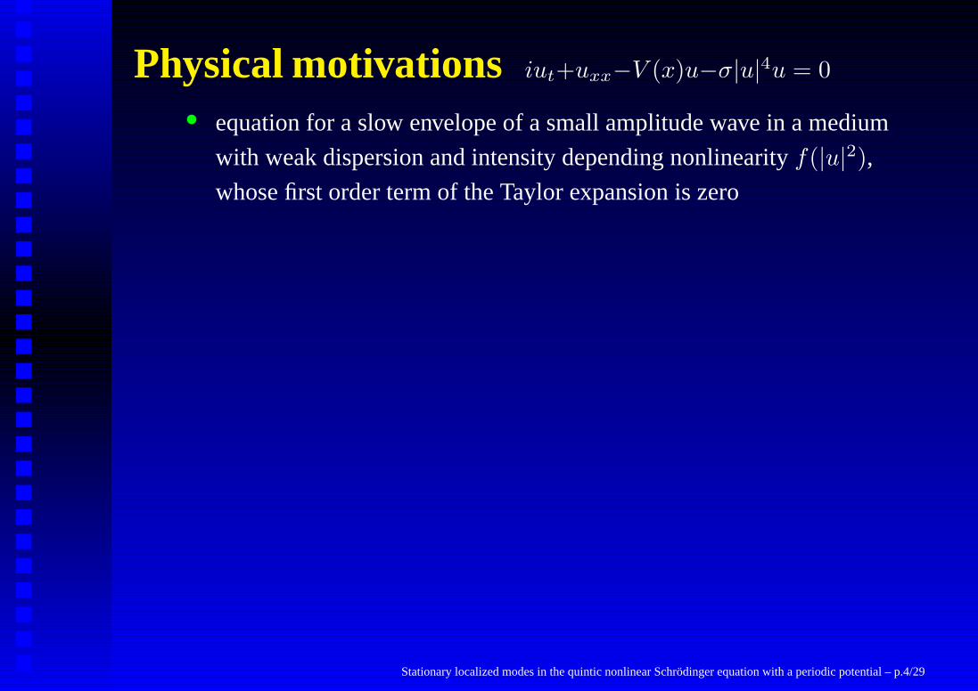
Physical motivations iut+uxx−V (x)u−σ|u|4u = 0



• equation for a slow envelope of a small amplitude wave in a medium

with weak dispersion and intensity depending nonlinearityf(|u|2),whose first order term of the Taylor expansion is zero





• renewed interest was originated by suggestions of its use for description

of a one-dimensional gas of bosons

Kolomeisky, et. al., Phys. Rev. Lett.85, 1146 (2000)

M. D. Girardeau and E. M. Wright, Phys. Rev. Lett.84, 5239 (2000)

B. Damski, J. Phys. B37, L85 (2004)

J. Brand, J. Phys. B37, S287 (2004)





• renewed interest was originated by suggestions of its use for description

of a one-dimensional gas of bosons

Kolomeisky, et. al., Phys. Rev. Lett.85, 1146 (2000)

M. D. Girardeau and E. M. Wright, Phys. Rev. Lett.84, 5239 (2000)

B. Damski, J. Phys. B37, L85 (2004)

J. Brand, J. Phys. B37, S287 (2004)

• quasi-one-dimensional limit of the generalized Gross-Pitaevskii

equation when two-body interactions are negligibly small

Abdullaev, Salerno, Phys. Rev. A72, 033617 (2005)

Brazhnyi, Konotop, Pitaevskii, Phys. Rev. A73, 053601 (2006)


Physical motivations

The stationary version of the QNLS describes the ground state of

the so-called Tonks-Girardeau gas

L. Tonks, Phys. Rev.50, 955 (1936)

M. Girardeau, J. Math. Phys.1, 516 (1960)

and it has been justified in

E.H. Lieb, R. Seiringer, J. Yngvason, Phys. Rev. Lett.91, 150401

(2003)


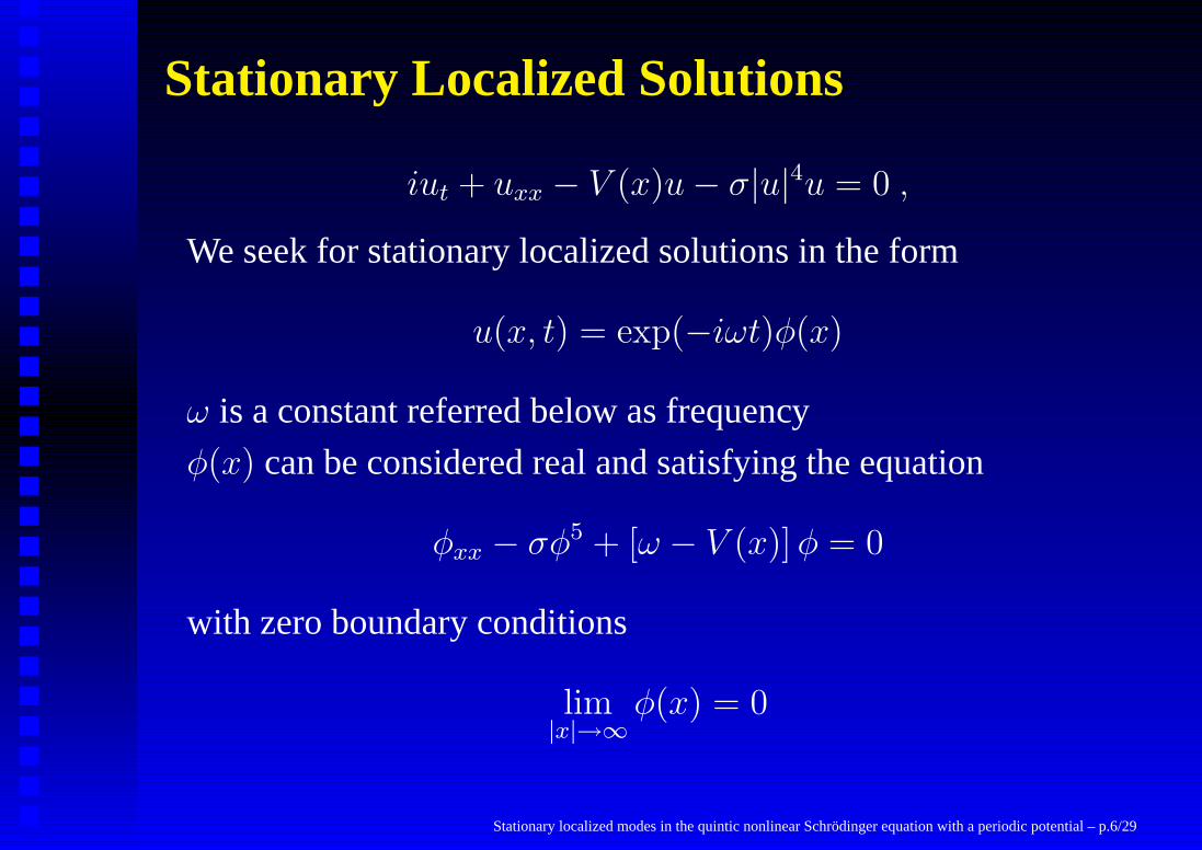
Stationary Localized Solutions

iut + uxx − V (x)u− σ|u|4u = 0 ,

We seek for stationary localized solutions in the form

u(x, t) = exp(−iωt)φ(x)

ω is a constant referred below as frequency

φ(x) can be considered real and satisfying the equation

φxx − σφ5 + [ω − V (x)]φ = 0

with zero boundary conditions

lim|x|→∞

φ(x) = 0


Linear eigenvalue problemThe asymptotics of a localized solution are determined by the

linear eigenvalue problem

d2ϕαq

dx2+ [ωα(q) − V (x)]ϕαq = 0


Linear eigenvalue problemThe asymptotics of a localized solution are determined by the

linear eigenvalue problem

d2ϕαq

dx2+ [ωα(q) − V (x)]ϕαq = 0

which has a band spectrumωα(q) ∈[

ω(−)α , ω

(+)α

]

α = 1, 2, . . . referring to a band number

“+” and “–” standing respectively for the upper and lower

boundaries of theα-th band.

ϕαq are Bloch functions andq is the wave number in the reduced

Brillouin zone,q ∈ [−1, 1].

An interval(

ω(+)α , ω

(−)α+1

)

represents theα’s gap.


Integrals of motionNumber of Particles

N =

∫

|u(x, t)|2dx



N =

∫

|u(x, t)|2dx

Energy functional

E =1

2

∫(

|ux|2 −1

3|u|6 + V |u|2

)

dx



N =

∫

|u(x, t)|2dx

Energy functional

E =1

2

∫(

|ux|2 −1

3|u|6 + V |u|2

)

dx

Remark: for σ = −1 andV (x) = 0 the numberN∗ =√

3π/2

separates the solutions which may collapse (N > N∗) and

solutions for which no collapse can occur (N < N∗)M. Weinstein, Comm. Math. Phys.87, 567 (1983)

G. Fibich and G. Papanicolaou, SIAM J. Appl. Math.60, 183 (1999)


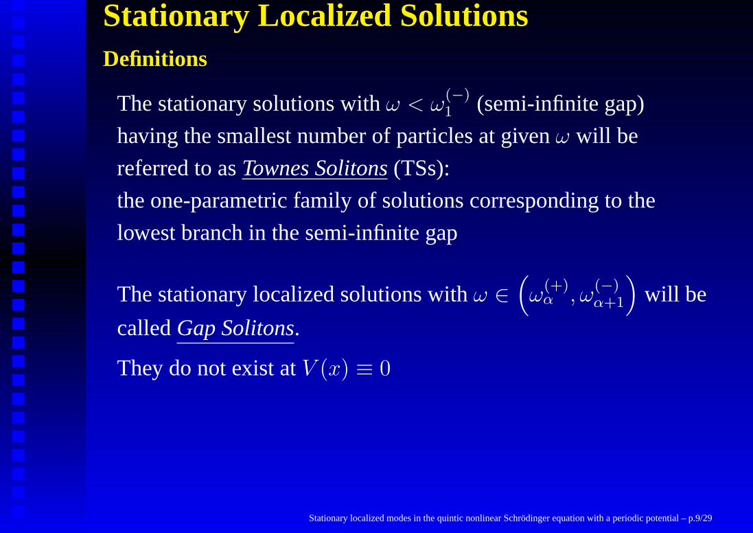
Stationary Localized SolutionsDefinitions

The stationary solutions withω < ω(−)1 (semi-infinite gap)

having the smallest number of particles at givenω will be

referred to asTownes Solitons(TSs):

the one-parametric family of solutions corresponding to the

lowest branch in the semi-infinite gap


Stationary Localized SolutionsDefinitions

The stationary solutions withω < ω(−)1 (semi-infinite gap)

having the smallest number of particles at givenω will be

referred to asTownes Solitons(TSs):

the one-parametric family of solutions corresponding to the

lowest branch in the semi-infinite gap

The stationary localized solutions withω ∈(

ω(+)α , ω

(−)α+1

)

will be

calledGap Solitons.

They do not exist atV (x) ≡ 0


Sufficient condition for collapse

in the attractive case (σ = −1)




y(t) =

∫

x2|u|2dx

z(t) = Im∫

xuuxdx ,




y(t) =

∫

x2|u|2dx

z(t) = Im∫

xuuxdx ,

Theorem– If the conditions

z(0) ≥ 0 and η = −4E0 − V1y1/2(0)N1/2 > 0 ,

whereE0 = E + V0N/2 and V1 = supx |Vx(x)|, are satis-

fied, theny(t) ≤ y(0) − 2η t2 and collapse occurs at finite time

T ≤ (y(0)/2η)1/2.


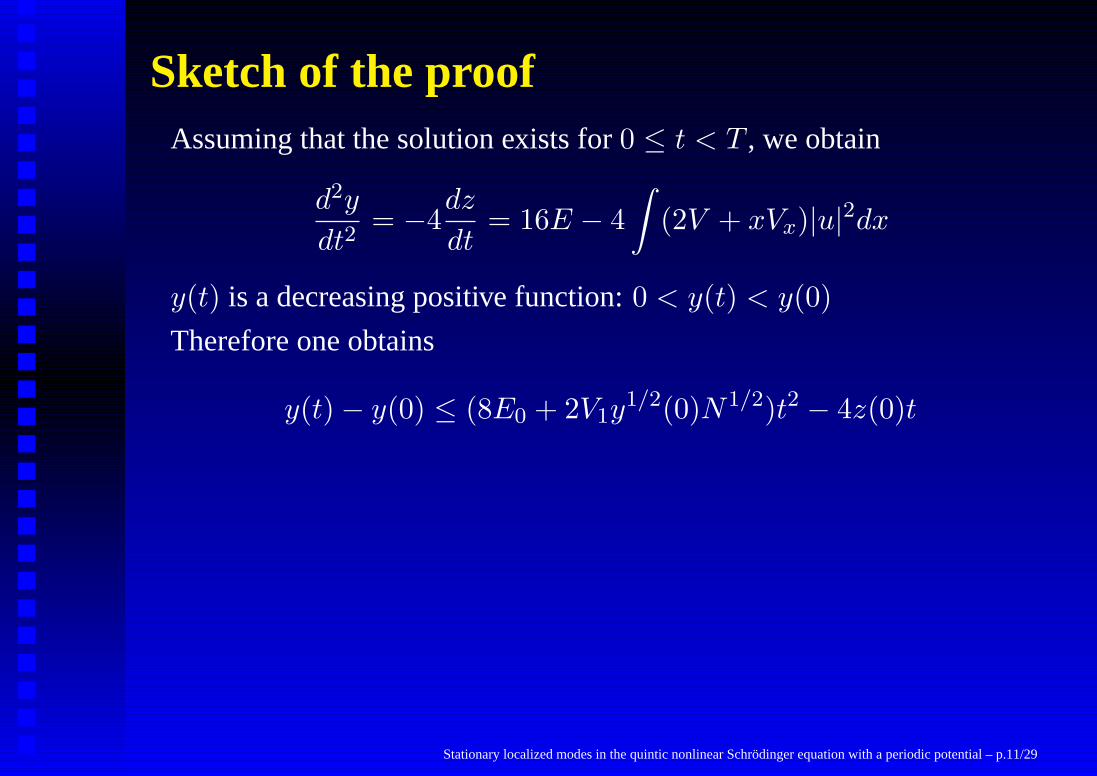
Sketch of the proofAssuming that the solution exists for0 ≤ t < T , we obtain

d2y

dt2= −4

dz

dt= 16E − 4

∫

(2V + xVx)|u|2dx

y(t) is a decreasing positive function:0 < y(t) < y(0)

Therefore one obtains

y(t) − y(0) ≤ (8E0 + 2V1y1/2(0)N1/2)t2 − 4z(0)t


Sketch of the proofAssuming that the solution exists for0 ≤ t < T , we obtain

d2y

dt2= −4

dz

dt= 16E − 4

∫

(2V + xVx)|u|2dx

y(t) is a decreasing positive function:0 < y(t) < y(0)

Therefore one obtains

y(t) − y(0) ≤ (8E0 + 2V1y1/2(0)N1/2)t2 − 4z(0)t

Remark: Comparing with the conditions for collapse for homoge-

neous caseV1 = 0 we conclude that in the presence of a periodic

potential the collapse occurs at smaller values of energyE < 0


Existence of a minimum N


Existence of a minimum N∫

φ2xdx ≤ (ω + V0)N

[

1 +3

2

N2

N2∗

(σ − 1)

]−1

[φ `

φxx − σφ5 + [ω − V (x)] φ = 0´

, integrating and using the Gagliardo-Nirenberg

inequality:R

φ6dx ≤ (3N2/N2∗)

R

φ2xdx]




[

1 +3

2

N2

N2∗

(σ − 1)

]−1

[φ `

φxx − σφ5 + [ω − V (x)] φ = 0´


inequality:R

φ6dx ≤ (3N2/N2∗)

R

φ2xdx]

• The stationary solutions atω < −V0 haveN > N∗/√

3

• Combining with the inequality(supx φ)4 ≤ 4N∫

φ2xdx

limit of small number of particles,N → 0, if available,

implies smallness of the amplitude of the function

supx |φ| → 0.




[

1 +3

2

N2

N2∗

(σ − 1)

]−1

[φ `

φxx − σφ5 + [ω − V (x)] φ = 0´


inequality:R

φ6dx ≤ (3N2/N2∗)

R

φ2xdx]

• The stationary solutions atω < −V0 haveN > N∗/√

3

• Combining with the inequality(supx φ)4 ≤ 4N∫

φ2xdx

limit of small number of particles,N → 0, if available,

implies smallness of the amplitude of the function

supx |φ| → 0.

Small amplitude limit of the QNLS

[V. A. Brazhnyi and V. V. Konotop, Mod. Phys. Lett. B18627 (2004)

and references therein]Stationary localized modes in the quintic nonlinear Schrodinger equation with a periodic potential – p.12/29

Minimal number of particlesWe look for a solution of the QNLS in a form

ψ = ǫ1/2ψ1 + ǫ3/2ψ2 + · · ·

ǫ≪ 1 andψj are functions of slow variablesxp = ǫpx, tp = ǫpt

ψ1 = A(x1, t2)ϕα(x0) exp(−iωαt0)

ωα stands either forω(+)α (if σ = 1) or for ω(−)

α+1 (if σ = −1) and

ϕα stands for the respective Bloch function.


Minimal number of particlesThe slow envelopeA(x1, t2) solves the QNLS equation

i∂A

∂t2+

1

2Mα

∂2A

∂x21

− σχα|A|4A = 0

χα =∫ π

0|ϕα(x)|6dx is theeffective nonlinearity

M−1α = d2ωα(q0)/dq

2 is theeffective mass(q0 = 0 andq0 = 1

for the center and the boundary of the Brillouin zone)



i∂A

∂t2+

1

2Mα

∂2A

∂x21

− σχα|A|4A = 0

The soliton solution is known:

A =31/4ǫ1/2

χ1/4α

exp(−iσǫ2t)√

cosh(

ǫx√

8|Mα|)



i∂A

∂t2+

1

2Mα

∂2A

∂x21

− σχα|A|4A = 0


A =31/4ǫ1/2

χ1/4α

exp(−iσǫ2t)√

cosh(

ǫx√

8|Mα|)

Thusǫ2 can be interpreted as a frequency detuning to the gap,

ǫ2 = |ω − ωα|



i∂A

∂t2+

1

2Mα

∂2A

∂x21

− σχα|A|4A = 0


A =31/4ǫ1/2

χ1/4α

exp(−iσǫ2t)√

cosh(

ǫx√

8|Mα|)

The number of particles

N ≈ N = ǫ

∫

|A|2dx =π√

3

2√

2|χαMα|

is determinedonlyby the lattice parametersStationary localized modes in the quintic nonlinear Schrodinger equation with a periodic potential – p.14/29


i∂A

∂t2+

1

2Mα

∂2A

∂x21

− σχα|A|4A = 0


A =31/4ǫ1/2

χ1/4α

exp(−iσǫ2t)√

cosh(

ǫx√

8|Mα|)

Note the difference with the case of nonlinear Schrödinger

equation with cubic nonlinear term: the number of particlesN

tends to zero together with the detuning:N ∝√

|ωα − ω|



i∂A

∂t2+

1

2Mα

∂2A

∂x21

− σχα|A|4A = 0


A =31/4ǫ1/2

χ1/4α

exp(−iσǫ2t)√

cosh(

ǫx√

8|Mα|)

The number of particles

N ≈ N = ǫ

∫

|A|2dx =π√

3

2√

2|χαMα|

is determinedonlyby the lattice parametersStationary localized modes in the quintic nonlinear Schrodinger equation with a periodic potential – p.14/29

Numerical results - Semi-infinity gap,σ = −1

ω

N

-1.3 -1.2 -1.1 -10.5

1

1.5

2

2.5

3

A

BC

D

ω∗

N*

xφ

-10 0 100

0.4

0.8 A

x

φ

-10 0 100

0.4

0.8B

x

φ

-100 0 100

0.1

0.2 C

x

φ

-20 0 200

0.25

0.5 D

ω(−)1 ≈ −0.9368

(A) ω = −1.2, (B) ω = −1.1, (C) ω = −0.9374, (D) ω = −0.95. ω∗ ≈ 1.0005

x

φ

-2 0 20

1

2 (a)ω

N

-12 -10 -82.2

2.4

2.6

2.8N*

ω

N

-12 -10 -84.4

4.8

5.2

5.62N*

x

φ

-4 -2 0 2 40

1

2 (b)ω

N

-12 -10 -86.8

7.6

8.43N*

x

φ

-4 -2 0 2 40

1

2 (c)

V0 = 1 solid line,V0 = 3 dashed line,V0 = 5 dotted line, corresponding to 1st, 2nd, 3rd

branches. In (a), (b), (c) the shapes of the solutions forV0 = 3 andω = −12.175



ω

N

-1.3 -1.2 -1.1 -10.5

1

1.5

2

2.5

3

A

BC

D

ω∗

N*

x

φ-10 0 100

0.4

0.8 A

x

φ

-10 0 100

0.4

0.8B

x

φ

-100 0 100

0.1

0.2 C

x

φ

-20 0 200

0.25

0.5 D



ω

N

-1.3 -1.2 -1.1 -10.5

1

1.5

2

2.5

3

A

BC

D

ω∗

N*

x

φ-10 0 100

0.4

0.8 A

x

φ

-10 0 100

0.4

0.8B

x

φ

-100 0 100

0.1

0.2 C

x

φ

-20 0 200

0.25

0.5 D

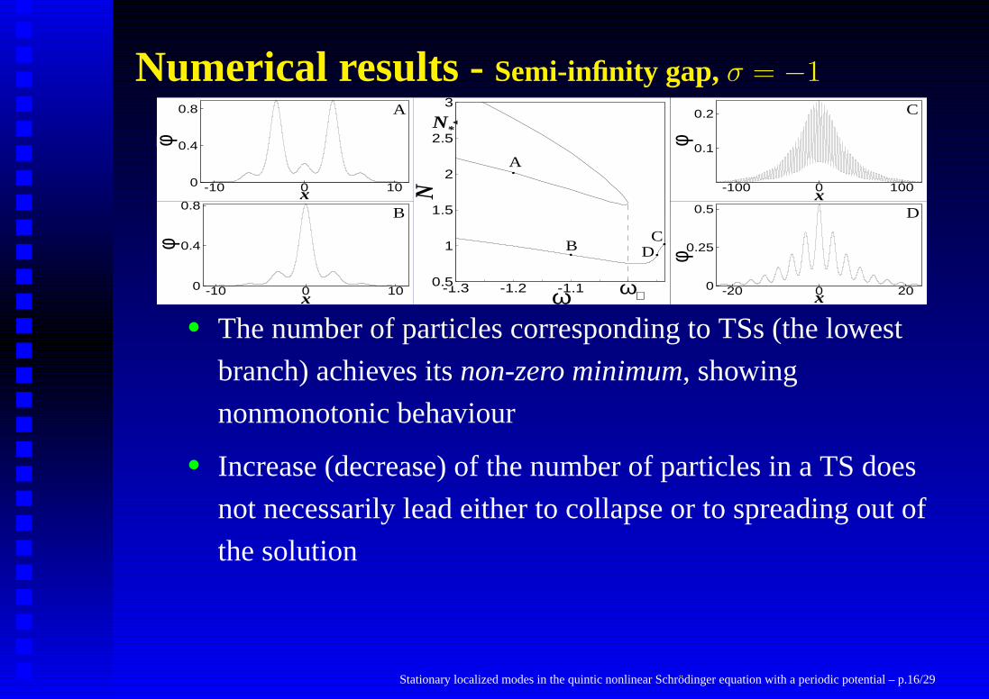
• The number of particles corresponding to TSs (the lowest

branch) achieves itsnon-zero minimum, showing

nonmonotonic behaviour



ω

N

-1.3 -1.2 -1.1 -10.5

1

1.5

2

2.5

3

A

BC

D

ω∗

N*

x

φ-10 0 100

0.4

0.8 A

x

φ

-10 0 100

0.4

0.8B

x

φ

-100 0 100

0.1

0.2 C

x

φ

-20 0 200

0.25

0.5 D

• The number of particles corresponding to TSs (the lowest

branch) achieves itsnon-zero minimum, showing

nonmonotonic behaviour

• Increase (decrease) of the number of particles in a TS does

not necessarily lead either to collapse or to spreading out of

the solution



ω

N

-1.3 -1.2 -1.1 -10.5

1

1.5

2

2.5

3

A

BC

D

ω∗

N*

x

φ-10 0 100

0.4

0.8 A

x

φ

-10 0 100

0.4

0.8B

x

φ

-100 0 100

0.1

0.2 C

x

φ

-20 0 200

0.25

0.5 D

• Existence of the local minimum on the lowest curveN(ω),

at a frequency shifted from the edge toward the gap, does

not contradict the small amplitude approximation. The

small parameterǫ1/2 ∼ 0.1 corresponds to the frequency

detuning|ω − ωα| ∼ 10−4, therefore the region of validity

of asymptotic expansions is very narrow: the reshaping of a

soliton from the envelope soliton in C to an intrinsic

localized mode in B occurs already at quite small frequency

detuning Stationary localized modes in the quintic nonlinear Schrodinger equation with a periodic potential – p.16/29


ω

N

-1.3 -1.2 -1.1 -10.5

1

1.5

2

2.5

3

A

BC

D

ω∗

N*

x

φ-10 0 100

0.4

0.8 A

x

φ

-10 0 100

0.4

0.8B

x

φ

-100 0 100

0.1

0.2 C

x

φ

-20 0 200

0.25

0.5 D

• The whole lower branch lies below the critical valueN∗.

This means that, unlike the homogeneous QNLS equation,

small enough perturbations of stationary solutions in

presence of a periodic lattice do not result in collapsing

behaviour



ω

N

-1.3 -1.2 -1.1 -10.5

1

1.5

2

2.5

3

A

BC

D

ω∗

N*

x

φ-10 0 100

0.4

0.8 A

x

φ

-10 0 100

0.4

0.8B

x

φ

-100 0 100

0.1

0.2 C

x

φ

-20 0 200

0.25

0.5 D

• In the cubic nonlinear Schrödinger equation the number of

particles is a monotonic function of the frequency detuning:

Aα ∝ |ω − ωα|1/2 and the small parameter isε instead of

ε1/2 obtained above



x

φ

-2 0 20

1

2 (a)ω

N

-12 -10 -82.2

2.4

2.6

2.8N*

ω

N

-12 -10 -84.4

4.8

5.2

5.62N*

x

φ

-4 -2 0 2 40

1

2 (b)ω

N

-12 -10 -86.8

7.6

8.43N*

x

φ

-4 -2 0 2 40

1

2 (c)



x

φ

-2 0 20

1

2 (a)ω

N

-12 -10 -82.2

2.4

2.6

2.8N*

ω

N

-12 -10 -84.4

4.8

5.2

5.62N*

x

φ

-4 -2 0 2 40

1

2 (b)ω

N

-12 -10 -86.8

7.6

8.43N*

x

φ

-4 -2 0 2 40

1

2 (c)

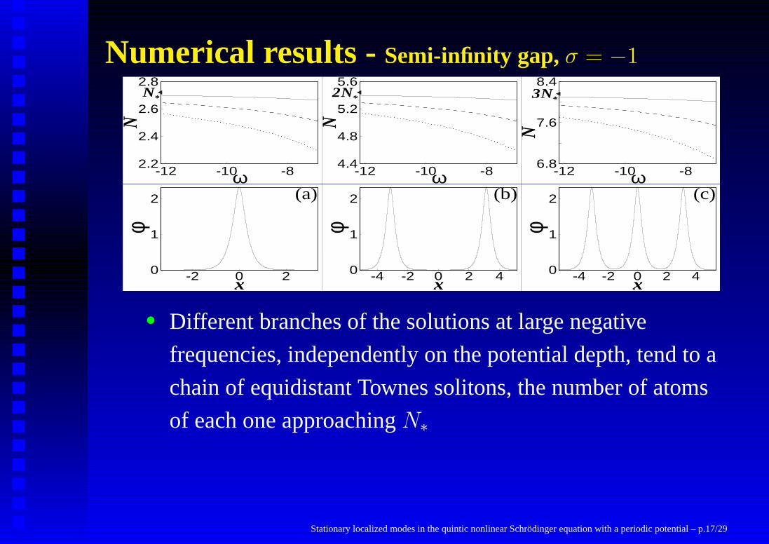
• Different branches of the solutions at large negative

frequencies, independently on the potential depth, tend toa

chain of equidistant Townes solitons, the number of atoms

of each one approachingN∗



x

φ

-2 0 20

1

2 (a)ω

N

-12 -10 -82.2

2.4

2.6

2.8N*

ω

N

-12 -10 -84.4

4.8

5.2

5.62N*

x

φ

-4 -2 0 2 40

1

2 (b)ω

N

-12 -10 -86.8

7.6

8.43N*

x

φ

-4 -2 0 2 40

1

2 (c)

• The lowest branch solution has its counterpart for the

homogeneous QNLS equation, the coupled solitonic states

of the higher branches do not exist atV (x) ≡ 0. This

means that a lattice of arbitrary depth can be treated as a

singular perturbation allowing soliton binding



x

φ

-2 0 20

1

2 (a)ω

N

-12 -10 -82.2

2.4

2.6

2.8N*

ω

N

-12 -10 -84.4

4.8

5.2

5.62N*

x

φ

-4 -2 0 2 40

1

2 (b)ω

N

-12 -10 -86.8

7.6

8.43N*

x

φ

-4 -2 0 2 40

1

2 (c)

• Conjecture: "quantization" of the number of particles.

In the limitω → −∞ there exists an infinite number of

different stationary solutions of the QNLS equation with a

periodic potential, each of them havingnN∗, number of

particles (wheren is an integer). Thus there exist no upper

bound on the number of particles which can be loaded in

lattice Stationary localized modes in the quintic nonlinear Schrodinger equation with a periodic potential – p.17/29

Stability - Semi-infinity gap,σ = −1

x

φ

-2 0 20

1

2 (a)ω

N

-12 -10 -82.2

2.4

2.6

2.8N*

ω

N

-12 -10 -84.4

4.8

5.2

5.62N*

x

φ

-4 -2 0 2 40

1

2 (b)ω

N

-12 -10 -86.8

7.6

8.43N*

x

φ

-4 -2 0 2 40

1

2 (c)

Intoducing a perturbation of the initial form(1 + δ)φ(x), whereδ

was±0.01 andφ(x) was given by one of the distributions shown

in the figure we did not observe any significant change in the be-

haviour of the modes


Stability - Semi-infinity gap,σ = −1

ω

N

-1.3 -1.2 -1.1 -10.5

1

1.5

2

2.5

3

A

BC

D

ω∗

N*

x

φ-10 0 100

0.4

0.8 A

x

φ

-10 0 100

0.4

0.8B

x

φ

-100 0 100

0.1

0.2 C

x

φ

-20 0 200

0.25

0.5 D

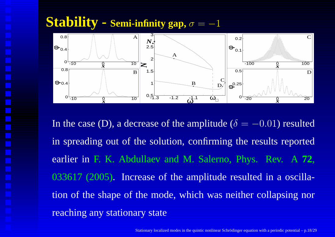
In the case (D), a decrease of the amplitude (δ = −0.01) resulted

in spreading out of the solution, confirming the results reported

earlier in F. K. Abdullaev and M. Salerno, Phys. Rev. A72,

033617 (2005). Increase of the amplitude resulted in a oscilla-

tion of the shape of the mode, which was neither collapsing nor

reaching any stationary state


Gap Solitons -first gap ω(+)1 ≈ −0.733, ω

(−)2 ≈ 2.1659

ω

N

0 1 23

4.5

6

7.5

9

A

B

CD

ω∗

xφ

-10 0 10-1

0

1 A

x

φ

-50 0 50

-1

0

1 Bx

φ

-50 0 50-0.5

0

0.5 C

x

φ

-10 0 10-1

0

1 D

σ = −1, even solutions(A) ω = 1.26, (B) ω = −0.73, (C) ω = 2.15, (D) ω = 1.33. ω∗ ≈ 1.256

ω

N

0 1 20

3

6

9

AB

C

D

N*

x

φ

-30 0 30-0.6

0

0.6 A

x

φ

-60 0 60-0.3

0

0.3 Bx

φ

-90 0 90

0

1C

x

φ

-15 0 15

0

0.5

D

σ = +1, odd solutions(A) ω = −0.7105, (B) ω = −0.73, (C) ω = 2.16, (D) ω = −0.5


Gap Solitons -first gap

ω

N

0 1 23

4.5

6

7.5

9

A

B

CD

ω∗

xφ

-10 0 10-1

0

1 A

x

φ

-50 0 50

-1

0

1 Bx

φ

-50 0 50-0.5

0

0.5 C

x

φ

-10 0 10-1

0

1 D

ω

N

0 1 20

3

6

9

AB

C

D

N*

x

φ

-30 0 30-0.6

0

0.6 A

x

φ

-60 0 60-0.3

0

0.3 Bx

φ

-90 0 90

0

1C

x

φ

-15 0 15

0

0.5

D

• One observes nonzero minima for the number of particles,

which are necessary for creation of gap solitons and

achieved at nonzero detuning toward the gap


Gap Solitons -first gap

ω

N

0 1 23

4.5

6

7.5

9

A

B

CD

ω∗

xφ

-10 0 10-1

0

1 A

x

φ

-50 0 50

-1

0

1 Bx

φ

-50 0 50-0.5

0

0.5 C

x

φ

-10 0 10-1

0

1 D

ω

N

0 1 20

3

6

9

AB

C

D

N*

x

φ

-30 0 30-0.6

0

0.6 A

x

φ

-60 0 60-0.3

0

0.3 Bx

φ

-90 0 90

0

1C

x

φ

-15 0 15

0

0.5

D

• One observes nonzero minima for the number of particles,

which are necessary for creation of gap solitons and

achieved at nonzero detuning toward the gap

• The number of particles for the localized modesgrows

infinitelywhen frequency approaches one of the gap edges.

This phenomenon is explained by thealgebraicasymptotic

of the gap soliton, which corresponds to the border of the

band:φ ∝ 1/x1/2 asx→ ∞


Gap Solitons - AsymptoticsLet us denote byωα the respective gap boundary, such that

ωα = ω(−)α+1 if σ = 1 andωα = ω

(+)α if σ = −1

Let ϕ0 be the periodic Bloch function corresponding toωα,

ϕ0(x) = ϕ0(x+ 2π), normalized by the relation∫ 2π

0ϕ2

0dx = 1.

We seek a solution in the form of the formal asymptotic series

φ = γ( ϕ0

x1/2+

ϕ1

x3/2+

ϕ2

x5/2+ · · ·

)

whereγ is a constant to be found.


Gap Solitons - AsymptoticsRecurrent formula forϕn (n = 1, 2...), the first step of which

leads tod2ϕ1

dx2+[ ϕ1

x3/2− V (x)

]

ϕ1 =dϕ0

dx

A solution of this equation can be represented in the form

ϕ1 = ϕ1(x) + c1ϕ0(x)

c1 is a constant

ϕ1 satisfies the orthogonality condition∫ 2π

0

ϕ1ϕ0 = 0


Gap Solitons - Asymptotics

Considering the terms proportional tox−5/2, we obtain

d2ϕ2

dx2+ [ωα − V (x)]ϕ2 = σγ4ϕ5

0 + 3dϕ1

dx− 3

4ϕ0

for which the orthogonality condition yields

σγ4

∫ 2π

0

ϕ60(x)dx+

3

4

∫ π

0

ϕ20dx− 3

∫ 2π

0

ϕ0dϕ1

dxdx = 0

Taking into account the representation ofϕ(x) as well as

normalization condition forϕ0 we compute

γ =

(

3σ1 − 4

∫ 2π

0ϕ1

ϕ0

dxdx

4∫ 2π

0ϕ6

0dx

)1/4


Gap Solitons - AsymptoticsNext, representingϕ2 = ϕ2 + c2ϕ0, considering the terms

corresponding tox−7/2 we obtain

d2ϕ3

dx2+ [ωα − V (x)]ϕ3 = 5

dϕ2

dx− 5γ4ϕ4

0ϕ1 −15

4ϕ1

From the orthogonality condition we obtain the coefficientc1


Gap Solitons - AsymptoticsContinuing the described procedure yields the terms of the

expansion forφ up to any order and all of them are

unambiguously defined.





The logarithmicdivergence of the number of particlesN takes

place asω → ωα,





The logarithmicdivergence of the number of particlesN takes

place asω → ωα,

Remark: a similar expansion for the cubic NLS equation gives the

decay∝ x−1, which implies finiteness of the number of particles

for the solution on the gap boundary.


Stability - first gap, σ = −1

ω

N

0 1 23

4.5

6

7.5

9

A

B

CD

ω∗

x

φ-10 0 10

-1

0

1 A

x

φ

-50 0 50

-1

0

1 Bx

φ

-50 0 50-0.5

0

0.5 C

x

φ

-10 0 10-1

0

1 D

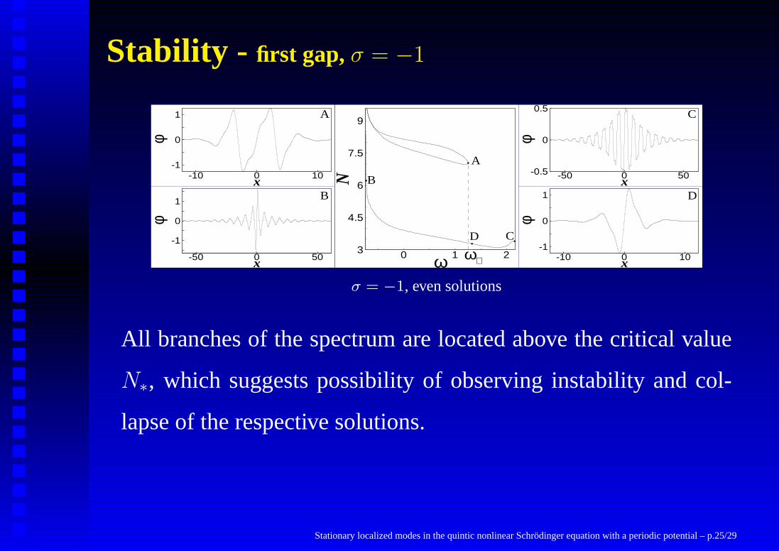
σ = −1, even solutions

All branches of the spectrum are located above the critical value

N∗, which suggests possibility of observing instability and col-

lapse of the respective solutions.


Stability - first gap

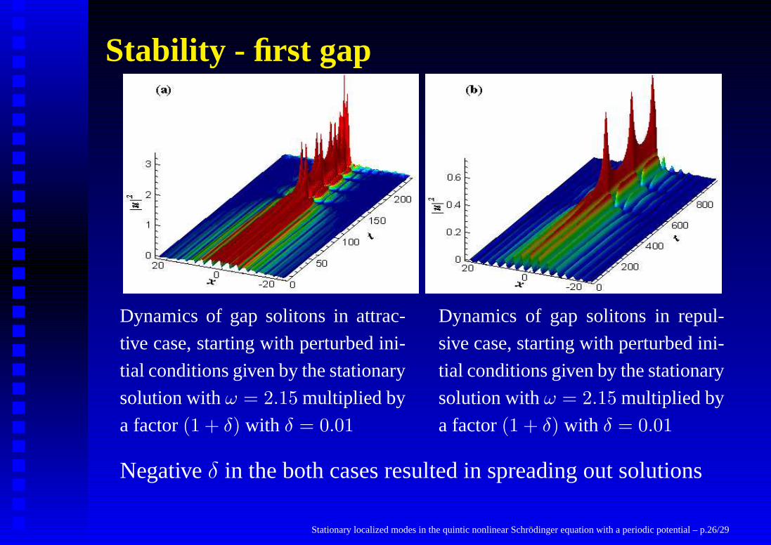
Dynamics of gap solitons in attrac-

tive case, starting with perturbed ini-

tial conditions given by the stationary

solution withω = 2.15 multiplied by

a factor(1 + δ) with δ = 0.01

Dynamics of gap solitons in repul-

sive case, starting with perturbed ini-

tial conditions given by the stationary

solution withω = 2.15 multiplied by

a factor(1 + δ) with δ = 0.01

Negativeδ in the both cases resulted in spreading out solutions





The dynamics shows three different stages of evolution, the first two

being similar for both attractive and repulsive cases.



Growth of the amplitudes and shrinking of the width of the solutions.

This "quasi-collapse" behavior is explained by the fact that in both

cases the dynamics is approximately described by the equation

i ∂A∂t2

+ 12Mα

∂2A∂x2

1− σχα|A|4A = 0, which is also an effective QNLS

equation, and thus corresponds to collapsing solutions.



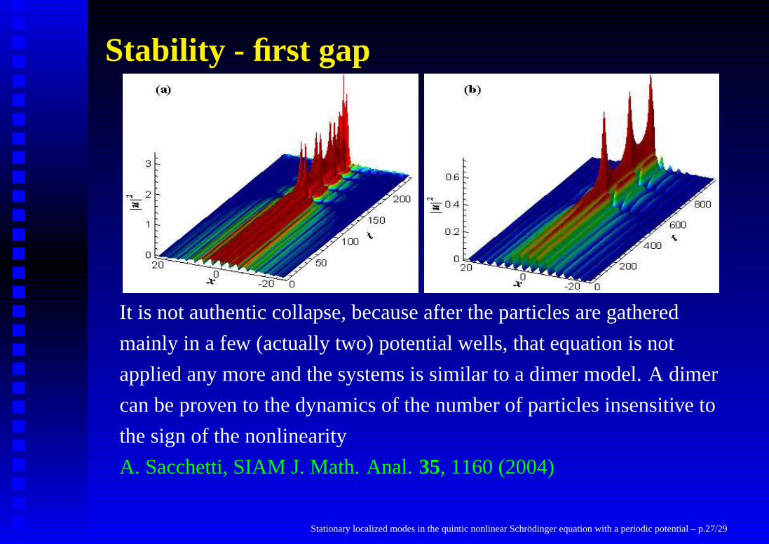
It is not authentic collapse, because after the particles are gathered

mainly in a few (actually two) potential wells, that equation is not

applied any more and the systems is similar to a dimer model. A dimer

can be proven to the dynamics of the number of particles insensitive to

the sign of the nonlinearity

A. Sacchetti, SIAM J. Math. Anal.35, 1160 (2004)



After several oscillations in attractive case we observed collapse. In the

repulsive case oscillatory behaviour was observed for longer times, also

showing three typical stages of the evolution, the first and second ones

being the same as in the attractive case and the last one corresponding

to decay of the pick amplitude and spreading out of the pulse


ConclusionsThe presence of the periodic potential results in qualitative

changes in behavior of the QNLS:



changes in behavior of the QNLS:• it modifies the sufficient condition for the collapse,

requiring negative energies with larger absolute values




requiring negative energies with larger absolute values• it allows the existence of infinite families of the localized

solutions





solutions• it can bind Townes solitons (the latter expressed by the

conjecture about quantization of the number of particles in

the limit of large negative frequencies)







the limit of large negative frequencies)• it allows storage of an infinite number of atoms, either by

coupling Townes soliton or by allowing existence of gap

solitons







the limit of large negative frequencies)• it allows storage of an infinite number of atoms, either by

coupling Townes soliton or by allowing existence of gap

solitons• it enforces the stability of Townes solitons allowing them to

have under-critical number of particlesStationary localized modes in the quintic nonlinear Schrodinger equation with a periodic potential – p.28/29

ConclusionsThe localized modes were shown to be very different from their

counterpart in the cubic nonlinear Schrödinger equation, where

the number of particles can go to zero and is bounded from

above.

The localized modes in the quintic nonlinear Schrödinger

equation

• require a minimal nonzero number of particles

• may have arbitrarily large number of atoms


Date post:	15-Feb-2019
Category:	Documents
Upload:	ngokhanh
View:	215 times
Download:	0 times

Stationary localized modes in the quintic nonlinear ... · G. L. Alﬁmov 1, V. V. Konotop2 and P....

Documents